A Preliminary Look at the Physics Reach of a Solar Neutrino TPC: Time-Independent Two Neutrino Oscillations

Contributed to Snowmass 2001, The Future of Particle Physics

Abstract

Solar neutrino physics below 2 MeV is a new frontier in particle and astrophysics. More than 99% of the solar neutrinos are produced in that region, and the physics output of a successful experiment includes stringent tests of stellar interior models. The original motivation to study solar neutrinos 40 years ago was indeed the study of the Sun’s interior. Even more important, from a particle physics perspective, is the opportunity to study neutrino mixing using a well-calibrated neutrino source that produces pure $\nu_{e}$ at $t=0$. This high intensity solar neutrino source allows sensitivity to neutrino masses down to $10^{-11}eV^{2}$, and it may produce enhanced sensitivity to neutrino mixing parameters via the strongly non-linear MSW effect.

This paper will discuss the physics reach of a solar neutrino TPC containing many tons of ${}^{4}\!{\rm He}$ under high pressure. Particular attention is given to the LMA and SMA solutions, which are allowed by current data[1], and which are characterized by a lack of time-dependent phenomena (either summer-winter or day-night asymmetries). In this case, the physics of neutrino masses and mixing is all contained in the energy dependence of the electron neutrino survival probability, $P_{e}(E)$ (or in its reciprocal, the electron neutrino disappearance probability, $P_{x}(E)=1-P_{e}(E)$). While it is clear that the $P_{e}(E)$ functions considered here cannot be the correct ones, due to the presence of a third neutrino, the physics reach of the TPC is analyzed within the context of the model to initiate a comparison between experiments. In Section 1 the observables available to a TPC are discussed. Section 2 describes the simulation methods, analysis and input parameters, and illustrates some qualitative features of the TPC capability using only the reconstructed neutrino energy. Section 3 presents more advanced fits using both the recoil electron energy and the reconstructed neutrino energy.

1 The information content of a TPC

Experimentally one can in principle count four neutrino species below 2 MeV; $pp$, ${}^{7}\!{\rm Be}$, $pep$ and $NO$, where the CNO spectra are counted as one. For each species there is a $\nu_{e}$ flux $\Phi_{e}$, a $\nu_{x}$ flux $\Phi_{x}$ ($x=\mu,\tau$), and at least one energy dependent parameter describing the change of $P_{e}(E)$ across the spectrum of the species.

Figure 1: The solar neutrino detection scheme. The recoiling electron energy and direction are measured, and the neutrino energy is reconstructed according to Eq. 1. Only a small fraction of the solid angle around the solar axis is considered at any given time.

In our approach, the scattering of a solar neutrino off of a target electron ($\nu e\to\nu e$) results in a completely reconstructed electron track (Fig.1). From the simultaneous reconstruction of the electron recoil energy ($T_{e}$) and its angle with respect to the solar axis ($\theta_{\odot}$), the neutrino energy for each event is given by

$$E_{\nu}={mT_{e}\over p\cos{\theta_{\odot}}-T_{e}}~{}.$$ (1)

This results in a direct measurement of the neutrino energy spectrum, and can be compared with solar models combined with neutrino mixing models. The correlations between $T_{e}$ and $E_{\nu}$ can also be used to measure the neutrino flavor content (see Sec. 3). This method works best when $E_{\nu}\sim m$. At energies far higher than the electron mass the error propagation becomes unfavorable.

A TPC is currently being designed to measure electron tracks for $T_{e}>100$ keV. The lowest energy $100$ keV tracks travel several cm before stopping, providing adequate track lever arm. The $\nu e$ elastic scattering cross-section is known to better than 1%, which effectively eliminates any theoretical error on the solar flux measurement. Further, the effective imaging of the event provides many opportunities for precision calibration of the device. It is very important to know the detector resolution function precisely.

The two main kinematically constrained types of events that one can use to study the detector (there are several types one can use) are $\delta-$rays from cosmic rays and double events. Every ten cosmic rays will produce a $\delta-$ray with a kinetic energy $T_{e}$ in excess of 100 keV, and distributed like $1/T_{e}^{2}$. If the cosmic is extremely relativistic, and typical energies underground average 300 GeV, then the following relation between the electron kinetic energy, electron mass, and its angle with respect to the cosmic direction is

$$T_{e}=2m/\tan^{2}\theta_{e}~{}.$$ (2)

Because generally $T_{e}<m$, these electron tracks are at large angles and can be easily separated from the column of ionization from the cosmic ray. At 2500 mwe we expect $\sim 10^{6}$ such events per year, providing virtually unlimited tagged, quality calibration events.

Another type of calibration event, “double-Compton”, consists of a photon that Compton-scatters twice in the TPC and produces two usable tracks which are correlated in time and angle (see Fig.2). Eight quantities are recorded by the TPC (3-momentum of each electron and direction between two vertices) against five possible degrees of freedom. In the simplest possible application the intermediate photon (the one connecting the two electron tracks) is reconstructed at both vertices using Compton kinematics. The exact kinematic relation

$${p_{1}\cos\theta_{1}\over T_{1}}+{p_{2}\cos\theta_{2}\over T_{2}}=2~{},$$ (3)

can be compared with the measured quantities to provide an accurate energy calibration. The angles $\theta_{1,2}$ are with respect to the direction of the intermediate photon. With the background conditions described below, $\sim 10^{4}$ double-Compton events per year are expected

Figure 2: Double-Compton background events in the TPC. A gamma ray enters the TPC and scatters twice, producing two usable electron tracks.

The calibration is expected to be of such quality that the energy scale and resolution will be known to $\sim 1$%[3]. These techniques can also map out position and time-dependent non-uniformities in the detector response. Many simulations have demonstrated that the reconstructed neutrino energy resolution is dominated by the angular resolution of the electron track. A gas mixture which is Helium dominated provides very low multiple scattering, as well as the opportunity to cold-trap impurities.

The other fundamental reason to have directionality is, of course, the direct measurement of the backgrounds. Except for the 6.8% variation in the flux due to the Earth eccentricity, our neutrino source varies only in direction. As abundantly proven by Kamiokande, directionality allows precise measurements in the presence of relatively high backgrounds, and will be demonstrated in greater detail later in this study. In practice the detector is sensitive only to the statistical fluctuations in the background, and the statistical significance ultimately will depend on $S/\sqrt{B}$.

2 Simulated Energy Spectra and Backgrounds

The neutrino survival probabilities were computed by using the analytic formulae of Ref. [4], convoluting them over the neutrino production region and propagating them through solar matter with the density profile described by the SSM. The MSW-SMA region is, generally speaking, characterized by a strongly varying $P_{e}(E)$. The MSW-LMA region has a slow, continuous spectral distortion across the 0-2 MeV region. Fig. 3 shows $P_{e}(E)$ for a conveniently chosen central point in the SMA region, and for four points nearby corresponding to a 21% variation up and down in both mass and $\sin^{2}{2\theta}$. Fig. 4 does the same for the LMA region. Because no time-dependent effects are expected in this region, the most general analysis is done by studying the $(E_{\nu},x)$ scatter plot, where $x=T_{e}/T_{e}^{max}$.

Monte Carlo events were generated using the parameters listed in Table 1. Results are presented for exposures of 7 and 70 Ton-years, roughly corresponding to one and ten years of data taking.

Table 1: Parameters used in the simulations described in the text.

Parameter	Value
Exposure	7 & 70 ton-years
$\sigma_{T}/T$	0.05 at 100 keV
$\sigma_{\theta}$	$15^{\circ}$ at 100 keV
${}^{238}U$	$0.5~{}\mu$g
${}^{14}\!{\rm C}/^{12}\!{\rm C}$	$5\times 10^{-20}$g/g

Substantial electron-track simulations have been undertaken over the years[5], which include the effects of multiple-scattering and diffusion in a large static electric field. Amongst the recent results are the good agreement of various simulation packages (GEANT and FLUKA), and an estimate of the angular resolution which scales with pressure as $\sim 1/P^{2}$. A complete optimization of the tracking algorithm represents a genuinely new problem and will be part of our future R&D. Based on the results from these simulations, we use the following detector resolutions:

$${{\sigma_{T}}\over T}(T)={0.016\over\sqrt{T}}~{}~{}~{}~{}~{}~{}~{}~{}~{}~{}~{}~{}~{}~{}\sigma_{\theta}(T)={4.7^{\circ}\over T^{0.6}}$$ (4)

where $T$ is the electron kinetic energy in MeV. At the lowest track energy of 100 keV, this corresponds to resolutions of 5% for energy and $15^{\circ}$ for angle.

The backgrounds were simulated as follows:

• $0.5~{}\mu$g of ${}^{238}U$ in secular equilibrium with its decay products, and uniformly distributed on the inner TPC surface. For each ${}^{238}U$ decay, this results in 0.68 $\gamma$’s from ${}^{214}Pb$ and 1.31 $\gamma$’s from ${}^{214}Bi$ ; the total number of emitted $\gamma$’s is $4.3\times 10^{5}$ for 7 ton-years.

• 5$\times 10^{-20}$ ${}^{14}C/^{12}C$ in the methane quencher, which corresponds to a ${}^{14}\!{\rm C}/^{4}\!{\rm He}$ ratio of $5\times 10^{-22}$.

Further sources of background, such as

• ${}^{14}C$ in the TPC body (contributing both direct tracks and bremstrahlung photons),

• cosmic-generated backgrounds

have been discussed elsewhere[3] and found to be negligible. Radon contamination is assumed to be avoidable, because the helium methane mixture can be processed through a cold trap. This detector needs less than a few $\mu Bq/m^{3}$, whereas purities an order of magnitude lower have been achieved, for example by GNO[6]. The radon-trapping efficiency has been measured to scale approximately like $1/T^{2}$[6], implying a factor of about two loss in efficiency when operating the trap at the boiling point of methane, which is 112K.

Figure 3: The neutrino survival probability in the SMA region, as a function of neutrino energy. The solid line is always the same, and represents the calculation for the nominal point at $(\Delta m^{2}=0.97\times 10^{-5},\sin^{2}{2\theta}=0.97\times 10^{-3})$. The dashed lines represent points displaced from the nominal point by 21%, respectively above, to the left, to the right, and below the nominal point.

Figure 4: The neutrino survival probability in the LMA region, as a function of neutrino energy. The solid line is always the same, and represents the calculation for the nominal point at $(\Delta m^{2}=3.9\times 10^{-5},\sin^{2}{2\theta}=0.39)$. The dashed lines represent points displaced from the nominal point by 21%, respectively above, to the left, to the right, and below the nominal point.

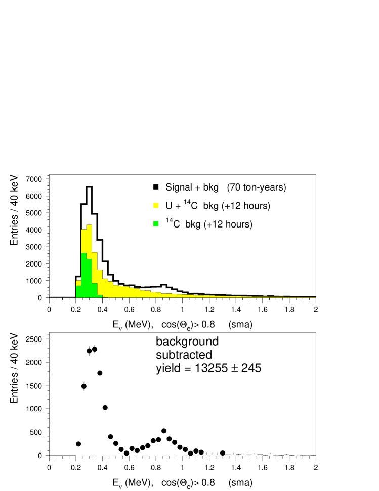
The expected rates in the TPC detector are shown in Table 2. The kinematic cut $\cos\theta_{\odot}>0.8$ retains 2/3 of the signal and improves the separation between the $pp$ and ${}^{7}\!{\rm Be}$ peaks (see Figure 5), and it also rejects 1/2 of the $U$-decay and 2/3 of the ${}^{14}\!{\rm C}$ background. The remaining background-rejection comes from requiring $T_{e}>0.1$ MeV and that the reconstructed neutrino energy is above 0.2 MeV. The typical signal rates are 1-2$\times 10^{3}$ per 7 ton-years, depending on the neutrino mixing solution, and the signal/background ratio is of order unity.

Using the SMA solution, an MC prediction of the “experimental” neutrino energy spectrum is shown in Figures 6-7 for 7 and 70 ton-years. The top plots show signal+background, and the shaded overlays show the background predictions based on events that point $180^{\circ}$ away from the sun; i.e., 12 hours out of phase. The bottom plots show the resulting $E_{\nu}$ “physics” spectrum after background-subtraction.

The TPC measurement capability is illustrated in Figures 8-10. Figure 8 compares the SMA and LMA solutions; there is some distinction with 7 ton-years and a very clear distinction with 70 ton-years. Additional information in $E_{\nu}$ vs. $T_{e}$ correlations give additional separation (see Sec. 3). Figure 9 shows the “experimental”/no-mixing ratio vs. $E_{\nu}$ for the LMA and SMA solutions. Note that $\nu_{\mu}e\to\nu_{\mu}e$ scattering in the TPC results in ratios that are slightly different than the $\nu_{e}$ survival probabilities in Figures 3-4.

Figure 10 compares two SMA solutions with slightly different values of $\Delta m^{2}$. The sensitivity to $\Delta m^{2}$ depends on the particular values of the neutrino mixing parameters, so the resulting uncertainty could be better or worse than the 20% $\Delta m^{2}$-difference shown in Figure 10.

Table 2: Rates per 7 ton-years for different neutrino mixing models and for backgrounds. “RAW” corresponds to electron events in the detector with no kinematic cuts. The “RAW U-decay+Compton” entry reflects $\gamma$’s that have Compton-scattered in the TPC, which is 7% of all $\gamma$’s from the U-decay chain. The rates are for $0.2<E_{\nu}<2.0$ MeV, where $E_{\nu}$ is the reconstructed neutrino energy. The LMA solution corresponds to $\Delta m^{2}=3.9\times 10^{-5}~{}{\rm eV}^{2},~{}{\rm sin}^{2}2\theta=0.39$; the SMA solution corresponds to $\Delta m^{2}=0.97\times 10^{-5}~{}{\rm eV}^{2},~{}{\rm sin}^{2}2\theta=0.00097$. Neutrino model or Rate per 7 ton-years: background source RAW after cuts SSM, no $\nu$ mixing $2.98\times 10^{3}$ $1.91\times 10^{3}$ SSM + MSW LMA $2.45\times 10^{3}$ $1.57\times 10^{3}$ SSM + MSW sma $2.04\times 10^{3}$ $1.31\times 10^{3}$ $U$-decay + Compton $3.27\times 10^{4}$ $1.67\times 10^{3}$ ${}^{14}\!{\rm C}~{}~{}~{}\beta$-decay $6.40\times 10^{4}$ $0.66\times 10^{3}$

Figure 5: Signal neutrino energy spectra (no background-subtraction) with different cuts on the cosine of the angle relative to the sun; no cut (dot-dash), $\cos\theta_{\odot}>0.6$ (dash), $\cos\theta_{\odot}>0.7$ (thick-dash), $\cos\theta_{\odot}>0.8$ (thick-line).

Figure 6: MC prediction for experimental neutrino energy spectrum based on 7 ton-years and with SMA solution ($\Delta m^{2}=0.97\times 10^{-5}~{}{\rm eV}^{2},~{}{\sin}^{2}2\theta=0.00097$). Top plot shows total spectrum with backgrounds, and bottom plot shows spectrum obtained after subtracting background based on events collected 12 hours out of phase.

Figure 7: MC prediction for experimental neutrino energy spectrum based on 70 ton-years and with SMA solution ($\Delta m^{2}=0.97\times 10^{-5}~{}{\rm eV}^{2},~{}{\sin}^{2}2\theta=0.00097$). Top plot shows total spectrum with backgrounds, and bottom plot shows spectrum obtained after subtracting background based on events collected 12 hours out of phase.

Figure 8: MC prediction of experimental neutrino energy spectrum for LMA (dots) and SMA (crosses) solutions. The top (bottom) plot corresponds to 7 (70) ton-years.

Figure 9: Ratio of predicted LMA $E_{\nu}$ spectrum to spectrum with no-mixing (top) and same for SMA solution (bottom). The statistical uncertainties are for 70 ton-years.

Figure 10: MC prediction of experimental neutrino energy spectrum for two SMA solutions with similar $\Delta m^{2}$ values as indicated on the plots (${\sin}^{2}2\theta=0.00097$ for both). The top (bottom) plot corresponds to 7 (70) ton-years.

3 Preliminary $(E,T)$ analysis

The number of measured events in {$E_{\nu},~{}T_{e}$} bins is related to the $\nu e$ scatter cross-sections by

$${{d^{2}N}\over{dE_{\nu}dT_{e}}} = P_{e}{d\sigma_{\nu_{e}e}\over dT_{e}}+(1-P_{e}){d\sigma_{\nu_{\mu}}\over dT_{e}}$$ (5)

$$= F_{1}-s(1-P_{e})F_{2}$$ (7)

where

$$F_{1}(E_{\nu},T_{e}) = (1/2+s)^{2}+s^{2}(1-T_{e}/E_{\nu})^{2}-s(1/2+s)\left(1-{{mT_{e}}\over{E_{\nu}^{2}}}\right)$$ (8)

$$F_{2}(E_{\nu},T_{e}) = 2-{{mT_{e}}\over{E_{\nu}^{2}}}$$ (9)

and $s=\sin^{2}\theta_{W}$.

Flavor separation by this method works best for the low energy $pp$ neutrinos. It works worst for ${}^{7}\!{\rm Be}$ neutrinos, because at those energies the two recoil spectra are very similar in shape. The strength of this method of analysis is in the model independent measurements that can be obtained by observing, on a statistical basis, both electron and non-electron neutrinos.

The elastic scatter cross section $\sigma(\nu_{x}e\to\nu_{x}e)$ is roughly 1/4 of $\sigma(\nu_{e}e\to\nu_{e}e)$, and the ratio varies slowly with energy. A change in $P_{e}$ with the energy $E$ is always accompanied by a change in the slope along $T$.

As mentioned above, if there is no observable time dependence in the solar neutrino flux, then all the information is obtained from the study of the scatter plot of any two quantities $\theta_{\odot}$, $T$ and $E$. Monte Carlo events were generated with large statistics (7000 Ton Years exposure, which is assumed to generate a negligible statistical error compared to the exposure of a real life experiment) on a fine grid (21$\times$21 points, with step size between 5% and 15%) on the $(\Delta M^{2},\sin^{2}{2\theta})$ plane. For each point on the grid, the $(E,T)$ distribution was recorded.

A further set of Monte Carlo events was generated, to be divided in simulated experiments of the appropriate exposure (7 or 70 ton Years). A binned likelihood function in $(E,T)$ was then used to compare the experiment under consideration with each point in the lattice, and the one with the best $\chi^{2}$ was found.

This method is rather simple, but it conveys an estimate of the physics reach of the detector when the recoil information is included. At the same time, it avoids the need to find an analytic fitting function, and does not need a parabolic $\chi^{2}$ (nearly impossible, given the strong non-linearity of the MSW effect) to converge.

Figs. 11 and 12 show the scatter of the best-fit points (100 simulated fits each), for a simulated exposure of 70 Ton Years, and background subtraction as described above. Drawn on the figure is the rough size of the currently 99% allowed LMA and SMA regions[1].

From the figures, one can infer the expected final error for this experiment, listed in Table3. Also listed is the approximate reduction factor in the $(\Delta M^{2},\sin^{2}{2\theta})$ log-log allowed region, compared to the current allowed regions.

Table 3: Physics reach of the TPC for an exposure of 70 Ton Years. All errors in percent of the central value.

Parameter	Value(%)
$\delta(\Delta M^{2})$, LMA	$\sim$ 30
$\delta(\Delta M^{2})$, SMA	3 to 10
$\delta(\sin^{2}2\theta)$, LMA	$\sim$ 7
$\delta(\sin^{2}2\theta)$, SMA	5 to 100
Reduction factor, LMA	$\sim 20$
Reduction factor, SMA	NA

Figure 11: SMA region: The result of 100 fits at three different values in ($\Delta M^{2},\sin^{2}2\theta$) using a statistics equivalent to 70 Ton-years of exposure. Backround subtraction as discussed in the text. The axes represent the logarithm of the usual $(\sin^{2}{2\theta},\Delta M^{2})$ values. The currently allowed region is drawn for comparison.

Figure 12: LMA region: The result of 100 fits using a statistics equivalent to 70 Ton-years of exposure. Background subtraction as discussed in the text have been subtracted. The axes represent the logarithm of the usual $(\sin^{2}{2\theta},\Delta M^{2})$ values. The currently allowed region is drawn for comparison.

Several comments are in order:

• according to Figs. 11 and 12, this detector would identify the correct region. In the LMA case, it would reduce the allowed region by about a factor of twenty. In some cases, some of the mixing parameters can be determined at the several percent level.

• this detector would allow extremely stringent checks of the sterile neutrino hypothesis. By measuring all types of neutrinos, in all flavors, it can compare directly against the solar luminosity to check that all solar energy is produced in association with neutrinos.

4 Conclusions

With strong evidence for long distance neutrino mixing[7], the next generation of experiments should aim for precision measurements of neutrino mixing parameters. The TPC detector described in this paper has the potential to dramatically reduce the allowed parameter space and to provide stringent test of the Standard Solar Model.

References

- [1] J. Bahcall, M. C. Gonzalez-Garcia and C. Pena-Garay, hep-ph/0106258.
- [2] J. Bahcall, Neutrino Astrophysics, Cambridge University Press, 1989, page 217.
- [3] F. Arzarello et al., LPC-94-28, CERN-LAA-94-19, Jul 1994.
- [4] M. Bruggen, W.C. Haxton, Y.-Z. Qian, Phys.Rev.D51:4028-4034,1995.
- [5] P. Gorodetzky et al., Nucl.Phys.Proc.Suppl.87:506-507,2000
- [6] C. Heusser, private communication.
- [7] Q. R. Ahmad et al., nucl-ex/0106015.