Astrophysical Neutrino Event Rates and Sensitivity for Neutrino Telescopes

Abstract

Spectacular processes in astrophysical sites produce high-energy cosmic rays which are further accelerated by Fermi-shocks into a power-law spectrum. These, in passing through radiation fields and matter, produce neutrinos. Neutrino telescopes are designed with large detection volumes to observe such astrophysical sources. A large volume is necessary because the fluxes and cross-sections are small. We estimate various telescopes’ sensitivities and expected event rates from astrophysical sources of high-energy neutrinos. We find that an ideal detector of km² incident area can be sensitive to a flux of neutrinos integrated over energy from $10^{5}$ and $10^{7}$ GeV as low as $1.3\times 10^{-8}\rm{E}^{-2}$ (GeV/cm² s sr) which is three times smaller than the Waxman-Bachall conservative upper limit on potential neutrino flux. A real detector will have degraded performance. Detection from known point sources is possible but unlikely unless there is prior knowledge of the source location and neutrino arrival time.

1 Introduction

Galactic and extra-galactic high-energy cosmic rays are observed at the Earth and in space through indicators such as synchrotron emission and gamma-radiation. Some of the most spectacular sites for their origin are the double-lobed radio sources associated with Active Galactic Nuclei. Figure 1 shows a compilation (Gaisser, 2000) of the observed cosmic ray spectrum observed at the Earth.

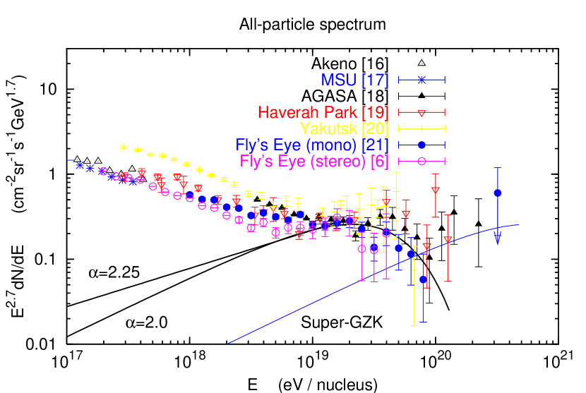
Figure 1: Cosmic Ray flux versus cosmic ray energy (extracted from (Gaisser, 2000)). Fits for two cosmic ray spectral indices ($\alpha$) are shown. The Super-GZK line refers to a possible contribution from nearby sources assuming $\alpha=2$ (see (Gaisser, 2000) for details.)

These high-energy cosmic rays interact with radiation or matter at the acceleration sites, in transit through intergalactic and interstellar space, and in the Earth’s atmosphere. Often the result of this interaction is the production of pions, kaons, and other particles that decay into muons and an associated muon neutrino. The muon will usually decay into an electron, an electron neutrino and a muon neutrino. Each primary cosmic ray interaction typically would produce at least three neutrinos and could produce substantially more.

One can estimate the flux of such neutrinos by models and from observations of the cosmic ray fluxes. One has to take into account the cosmic ray interactions which at high energies and from distant sources are primarily with photons. These estimates and fluxes must satisfy the limits set by the observations of cosmic rays. Another possibility to define the neutrino spectrum is given by the assumption that the high energy gamma-rays are produced by neutral pion decay. Under this assumption the high energy gamma-ray spectrum can be used to estimate the neutrino spectrum from charged pion decay. In this paper we estimate the muon neutrino and secondary muon flux from diffuse and point sources. The sources considered are the ones which are predicted to produce high energy (around $10^{19}$ eV) cosmic rays. Most models within the standard model of particle physics predict a muon neutrino rate that is at least twice the electron neutrino rate and even higher than the tau neutrino rate. The detector acceptance for muons is also higher than that for electrons and taus since muons can be detected even when created outside of the detector volume. For these reasons we only concentrate on the muon neutrino rate. Here we do not account for the flux due to exotic and beyond standard model possibilities but leave those topics for a later paper. A review of neutrino physics within and beyond the standard model can be found in (Learned and Mannheim, 2000).

There is strong evidence that neutrinos oscillate from one flavor to another Fukuda et al (1998) and that most likely muon neutrinos oscillate into tau neutrinos Fukuda et al (2000). Although this effect will lower the muon neutrino rate and enhance the one for tau neutrinos it is not taken into account in this work. We determine the most optimistic rates which are for muon neutrinos with no oscillation.

After reviewing estimates of neutrino fluxes we expand the previous work by including the fundamental physics aspects of instrument performance. This is done in a generic way that is independent of the detector configuration. We first determine the experimental sensitivity of an ideal detector of km² incident area to astrophysical sources and then translate this result to different detector geometries. Our results are compared to the sensitivity quoted by current and proposed experiments.

In Section 2 we review and examine estimates of high energy neutrino fluxes and upper limits from diffuse and point sources. We analyze Sagittarius (Sgr) A East as an example of a galactic point source and Gamma Ray Bursts and Active Galactic Nuclei as extra galactic point sources. These are good examples of the brightest sources. This section reviews the work of Waxman and Bahcall (Waxman, 1995; Waxman and Bahcall, 1999; Bahcall and Waxman, 2001), of Mannheim, Protheroe and Rachen (Mannheim Protheroe and Rachen, 2001) and the recent estimates by Gaisser (Gaisser, 2000). In Section 3 we compile and compute the interaction rates, that is, the neutrino interactions per unit volume per unit time and the number of muons entering or appearing in a generic detector. This work is directly compared to estimates by Gaisser (Gaisser, 2000). We then expand work previously done and determine the experimental sensitivity of an ideal detector to the muon rate. This is done in a generic form such that in Section 4 it is translated to different detector geometries. Realistic event rates are then determined for different proposed detectors such as IceCube, AMANDA, ANTARES and NESTOR.

2 Neutrino Fluxes

2.1 Diffuse Flux

2.1.1 Waxman and Bachall Limit

Waxman and Bahcall (WB) (Waxman and Bahcall, 1999; Bahcall and Waxman, 2001) pointed out that the observed cosmic ray flux at high energies implies an upper bound on the high-energy astrophysical neutrino flux. The latter is produced by the parent cosmic ray particles through pion production.

This argument holds for sources that are “optically thin” to the primary cosmic rays. “Optically thin” sources are those for which the majority of the protons escape and only a fraction interact inside the source. Observations of primary cosmic ray flux then set a limit on the cosmic production rate of high-energy protons and in turn on the production rate of neutrinos.

Waxman and Bachall also account for the cosmological evolution of the source activity and redshift energy loss of neutrinos due to cosmological expansion. If the cosmic ray acceleration sites were much more active in the past (billions of years) than in the present (last 100 million years), then the flux of “cosmological” high-energy neutrinos could be enhanced.

In determining a limit for the diffuse neutrino flux, WB assume that all the proton energy is transferred to the pion when actually this energy transfer is typically about 20%. Due to this factor, they point out that their upper bound exceeds what can be observed by at least a factor of five.

One can conclude that if the WB limit holds, the neutrino flux upper bound can guide neutrino telescope designs. Neutrino telescopes should be designed to detect realistic fluxes which would be at a level well below the WB limit.

The key parameter in setting an upper limit for the neutrino flux from the collection of “optically thin” sources, is the primary cosmic ray spectral index (which is the power in the power law energy distribution). For the relativistic shocks needed to produce the very highest energy cosmic rays the spectral index is in the range -2 to -2.5 (Bell, 1978; Blanford and Ostriker, 1978). Either will adequately explain what appears to be the extra-galactic component of the cosmic rays as shown in Figure 1.

Waxman (Waxman, 1995) has shown that the cosmic ray energy spectrum for energies between $10^{19}$ and $10^{20}$ eV is consistent with what is expected from a homogeneous cosmological distribution of cosmic ray sources and constrain the spectral index to be in the 1.8 – 2.8 range.

Fixing the spectral index to 2, WB (Waxman and Bahcall, 1999) determine the limit on muon neutrino plus muon anti-neutrino extra-galactic flux to be

$$\left(\frac{d\phi_{\nu}}{dE}\right)_{\rm limit}=\frac{1{\rm~{}to~{}}4\times 10^{-8}}{E^{2}}~{}~{}{\rm GeV\,cm^{-2}s^{-1}sr^{-1}}$$ (1)

where $\phi_{\nu}$ is the neutrino flux. Note that this limit is valid for sources that accelerate cosmic rays to above $10^{19}$ eV. The range in the coefficient depends upon what evolution is assumed. For this discussion we use the highest value and obtain an upper limit on the muon neutrino flux of

$$\left(\frac{d\phi}{dlnE}\right)_{\rm limit}=\frac{4\times 10^{-8}}{E}~{}~{}{\rm cm^{-2}s^{-1}sr^{-1}}$$ (2)

where E is given in GeV.

The WB limit is shown in Figure 2.

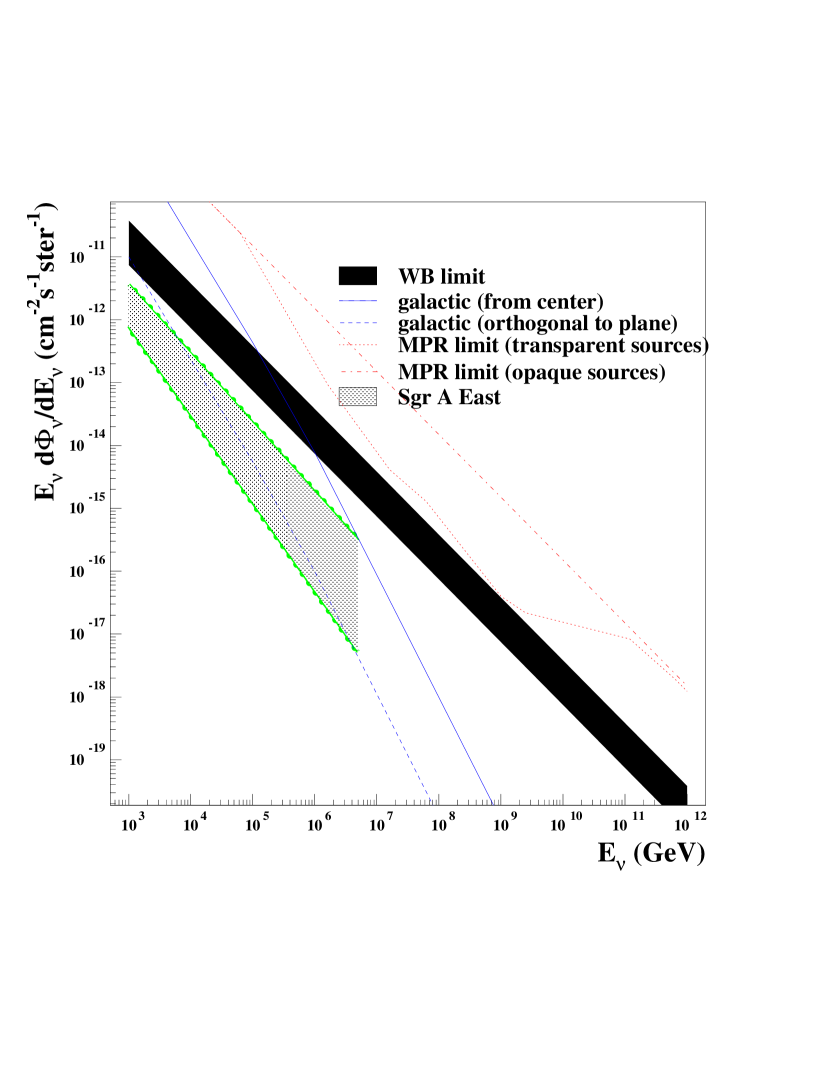
Figure 2: Differential neutrino fluxes weighted by neutrino energy from astrophysical sources and upper bound on the total diffuse neutrino flux. The lower edge of the dark shaded area is the WB limit (Waxman and Bahcall, 1999) with no cosmological evolution, the upper edge is the same limit taking evolution into account. The dashed line is the MPR (Mannheim Protheroe and Rachen, 2001) limit for transparent sources and the dotted dashed line for opaque sources. The continuous line is the flux from the Galactic center and the dashed line is the galactic flux from the direction orthogonal to the galactic plane (Ingelman and Thunman, 1996). The light shaded area is the neutrino flux from Sgr A East (Crocker et al., 2000) where the upper edge is the best case scenario flux and the lower edge is the worst case scenario (see text).

2.1.2 Mannheim, Protheroe and Rachen limit

Mannheim, Protheroe and Rachen (MPR) (Mannheim Protheroe and Rachen, 2001) determine an upper limit for diffuse neutrino sources in almost the same way as WB but with one important difference: they do not assume a specific cosmic ray spectrum but use the experimental upper limit on the extra-galactic proton contribution. While WB base their calculation on a cosmic ray flux with a single spectral index equal to -2, MPR define their spectrum based on current data at each energy.

MPR also extend their calculation for sources that are opaque (“optically thick”) to nucleons. For these sources they set an upper limit using the observed diffuse extra-galactic gamma-ray background assuming that the dominant part of the emitted gamma-radiation is in the Energetic Gamma Ray Experiment Telescope (EGRET, ) range.

Their results are also shown in Figure 2. Their limit for transparent (“thin”) sources is approximately the same as the WB limit for energies between $10^{7}$ and $10^{9}$ GeV and higher otherwise. Their limit allows the rates to be within the area defined by opaque and transparent sources. However, one should bear in mind that fluxes from opaque sources are difficult to produce. The interaction target in these sources must be optimized to allow interactions with most of the nucleons and at the same time allow pions and muons to decay. They also require an extraordinary larger energy budget than optically thin sources since a higher flux requires more energy. Also the opacity cuts down the flux of protons before they reach useful high energies implying a much larger initial flux and energy budget than the simple order of magnitude more flux would imply. As MPR state in their work, the WB limit is closer to current cosmic rays and neutrino production models. The opaque sources are in the “hidden” sources category.

2.1.3 “Hidden” Sources

The energy spectrum from opaque sources is not constrained by the observed cosmic ray flux (see section 2.1.1). Therefore models which predict such spectra are not limited by the WB derivation nor by the MPR for “thin” sources. These models assume sources that are “optically thick” to nucleons. The nucleons must first be accelerated to high energies and then encounter a target (radiation or matter) abundant enough to interact with most of the protons but low enough that the pions and muons are able to propagate freely and decay and then the neutrinos be allowed to escape. Berezinsky and Dokuchaev (Berezinsky and Dokuchaev, 2001) have proposed such a model and find that such a source could produce up to 10 muons crossing a one square kilometer area per year. One could argue that such a high flux would be limited to a short term (10 years out of billions) outburst. However, the long term limit for all sources is close to the WB limit.

Another model that assumes a source which is “optically thick” to nucleons has been proposed by Stecker et al (Stecker et al. 1991 and, 1992). It proposes that protons are accelerated to high energies in the AGN core. These protons produce neutrinos through photo-meson production. The neutrino flux predicted by this model is shown in Figure 4. A more recent version of this model (Stecker and Salamon, 1996) predicts a slightly different neutrino spectrum coming from quasars. Both predictions expect a neutrino flux at the level of the published AMANDA B-10 lower limit (Hill et al., 2001).

A way to avoid both the WB and MPR limits is the production of neutrinos in a way other than the photo-meson or proton-nucleon interactions. There is a vast list of models that can account for this possibility. A list of them can be found in (Bahcall and Waxman, 2001). Most of these involve new or “exotic” physics and we do not include them as “astrophysical” sources.

As discussed in section 2.1.2, neutrino fluxes from hidden sources are less likely to be produced.

2.1.4 GZK Fluxes

Very high-energy protons traveling through intergalactic space interact with the cosmic background photons and photo-produce pions. Greisen and Zatzepin and Kuz’min (Greisen 1966 and Zatsepin and Kuzmin, 1966) first pointed out that this process would occur and that it would set an upper bound to the maximum energy (a few times $10^{19}$ eV) for a proton traveling intergalactic distances (hundreds Mpc).

The production and flux of high energy neutrinos originated from intergalactic propagation of ultra high energy cosmic rays has been determined in (Engel and Stanev, 2001). They assume that the ultra-high energy cosmic rays are of astrophysical origin and show their result for different assumptions on cosmic ray source distributions, injection spectra and cosmological evolution. Their results with the same assumption for the injection power and cosmological evolution as Waxman and Bahcall (Waxman and Bahcall, 1999) are shown in Figure 3.

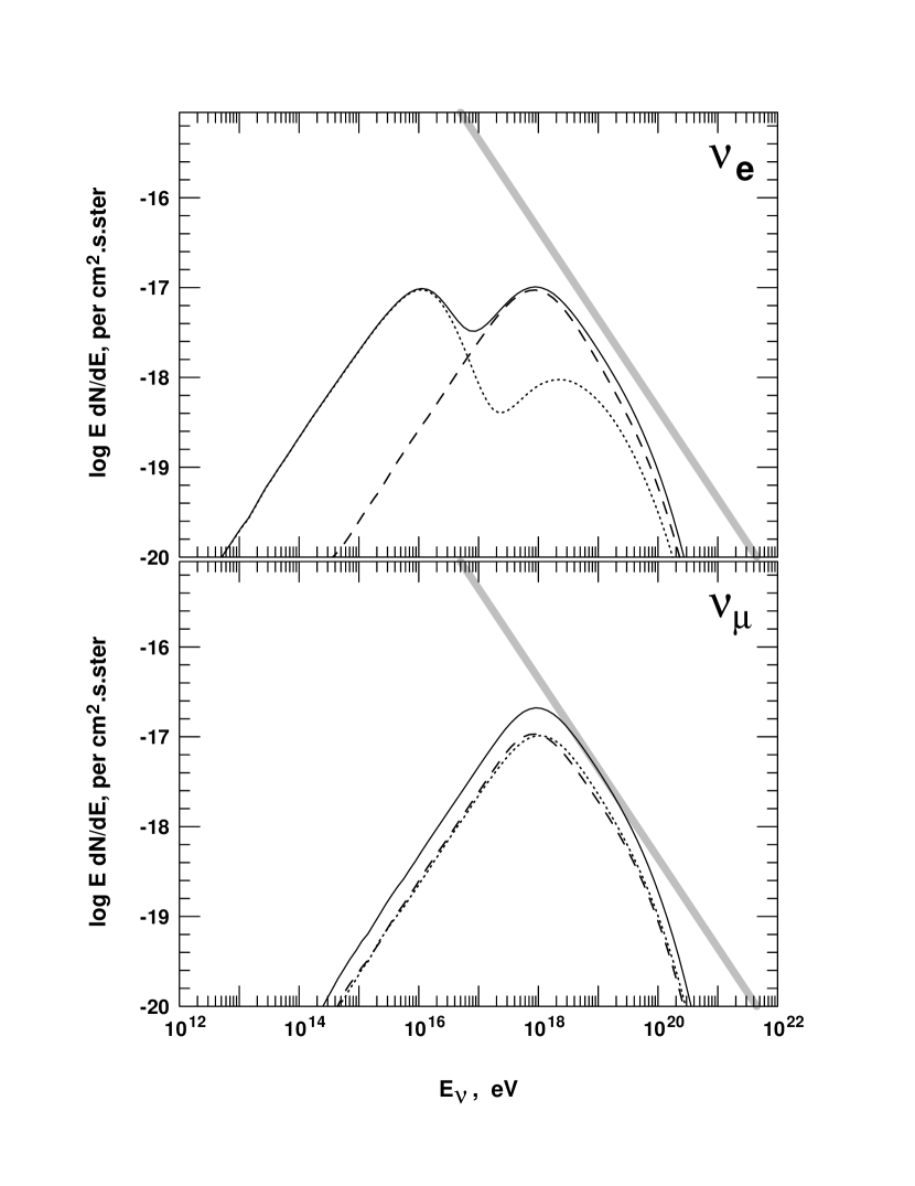
Figure 3: Differential fluxes weighted by neutrino energy of neutrinos generated by ultra high energy protons. Fluxes of electron neutrinos (dashed lines) and anti-neutrinos (dotted lines) are shown in the upper panel. The lower panel shows the fluxes of muon neutrinos and anti-neutrinos. Solid lines show the sum of neutrinos and anti-neutrinos. These fluxes were calculated in (Engel and Stanev, 2001) using the same injection power and cosmological source evolution as the WB limit (Waxman and Bahcall, 1999). This limit is represented by the shaded line. Figure extracted from (Engel and Stanev, 2001).

2.1.5 Neutrinos from the Galaxy

There is a significant diffuse flux of neutrinos created by interactions of the galactic and extra-galactic cosmic rays with interstellar matter and starlight. The spectrum of cosmic rays is reasonably well known, as is the distribution of targets in our Galaxy. We call the flux of neutrinos created by interactions in the interstellar medium the “galactic flux”.

Estimates of the galactic neutrino flux have been made by Domokos (Domokos, 1993), Berezinsky et al. (Berezinsky et al, 1993), and Ingleman and Thunman (Ingelman and Thunman, 1996). The diffuse galactic neutrino flux can be separated from the local atmospheric neutrino flux at energies above $10^{15}$ eV.

Above these energies the flux of diffuse galactic neutrinos stays harder than the atmospheric flux both because the original galactic cosmic rays have a harder spectrum nearer the center of the galaxy and most important the interstellar material is sufficiently thin and far away that the muons have adequate range and time to decay.

The muon neutrino flux (per GeV cm² sr s) is estimated (Ingelman and Thunman, 1996) by

$$\phi_{\nu}=\{\matrix{3.0\times 10^{-6}RE_{\nu}^{-2.63}~{}~{}~{}~{}~{}E_{\nu}<4.7\times 10^{5}~{}{\rm GeV}\cr 1.9\times 10^{-4}RE_{\nu}^{-2.95}~{}~{}~{}~{}~{}E_{\nu}>4.7\times 10^{5}~{}{\rm GeV}}$$ (3)

where $R$ is the distance to the edge of the galaxy in Kpc and E_ν is the neutrino energy in GeV.

The resulting flux from the direction of the center of the galaxy (20.5 kpc) and from the direction orthogonal to the galactic plane (0.26 kpc) are shown in Figure 2. Both the WB and MPR limits are for extra-galactic neutrinos.

One important point when considering the galactic flux is the direction from which the neutrinos come. Experiments in the South Pole will have an additional background from atmospheric muons when detecting neutrinos from the center of the galaxy since all events come from above the horizon. The atmospheric muon spectrum is steeper than the atmospheric neutrino spectrum  (Gaisser, 1990). The flux of atmospheric muons surviving to a depth of 1 km is 200 times larger than the atmospheric neutrino induced muons at 1 TeV. Furthermore, atmospheric muons that survive to kilometer depths are often produced in collimated bundles near the core of the parent cosmic-ray shower. Bundles of  10 TeV muons can easily be misidentified as a single high energy muon of 100 TeV or more. The spectral characteristics of muon bundles are not yet well characterized and lead to poor estimates of sensitivity above the horizon. For this reason we assume that atmospheric muons compose a irreducible background. In section 3.4 we determine the sensitivity for an expanded version of ANTARES (expanded to a km² incident area) to the neutrino flux from the galactic center.

2.2 Point Sources

In this section we consider sources that produce high-energy particles. Other than the hidden sources mentioned in section 2.1.3 active galactic nuclei (AGNs) and gamma-ray bursters are examples of extra galactic point sources. Other extragalactic point sources such as blazars (Dermer and Atoyan, 2001) (which compose a subclass of active galactic nuclei) might produce a lower flux of neutrinos when compared to GRBs. As an example of galactic point sources we show the neutrino flux from Sagittarius (Sgr) A East.

In principle a sufficiently bright point source can have their locations determined by the arrival direction of these particles (or by the particles produced by them) at the detector. The relevant issue is that, if the location of the source is pre-known, then the effective atmospheric background is effectively reduced by the ratio of the effective solid angles. The intrinsic angular deviation between the neutrino and daughter muon is of order $0.7^{\circ}/\sqrt{E_{\nu}/TeV}$ (Gaisser, 1990) so that the effective solid angle is of order one square degree. If the detector angular resolution is of this order, then the relative enhancement of signal-to-background can be as much as $10^{4}$.

2.2.1 Active Galactic Nuclei

Active Galactic Nuclei (AGN) are one of the brightest known astrophysical sources. They produce a multi-wavelength spectrum that goes from radio to TeV gamma rays. How such high-energy gammas are produced is still to be fully understood.

In the more conventional model high energy photons are produced by inverse Compton scattering of accelerated electrons on thermal UV photons (Sikora Begelman and Rees, 1994). This description is supported by multi-wavelength observations of Mkn 421 (Macomb et al 1995, 1996) although there are adjustments to be made (Halzen and Zas, 1997).

Other models (Mannheim, 1995; Halzen and Zas, 1997; Protheroe, 1996) describe the production of high energy gamma rays through the decay of photo produced neutral pions. These protons would be produced and accelerated in the AGN jet. This mechanism would be responsible for the production of the observed gamma-ray background.

Figure 4 shows that the non conventional model (Mannheim, 1995; Halzen and Zas, 1997; Protheroe, 1996) predictions are much higher than the WB limit. Waxman and Bahcall (Bahcall and Waxman, 2001) show that the sources in these models are optically thin and therefore should be constrained by their limit. They conclude that at least one of the basic assumptions of these models is not valid.

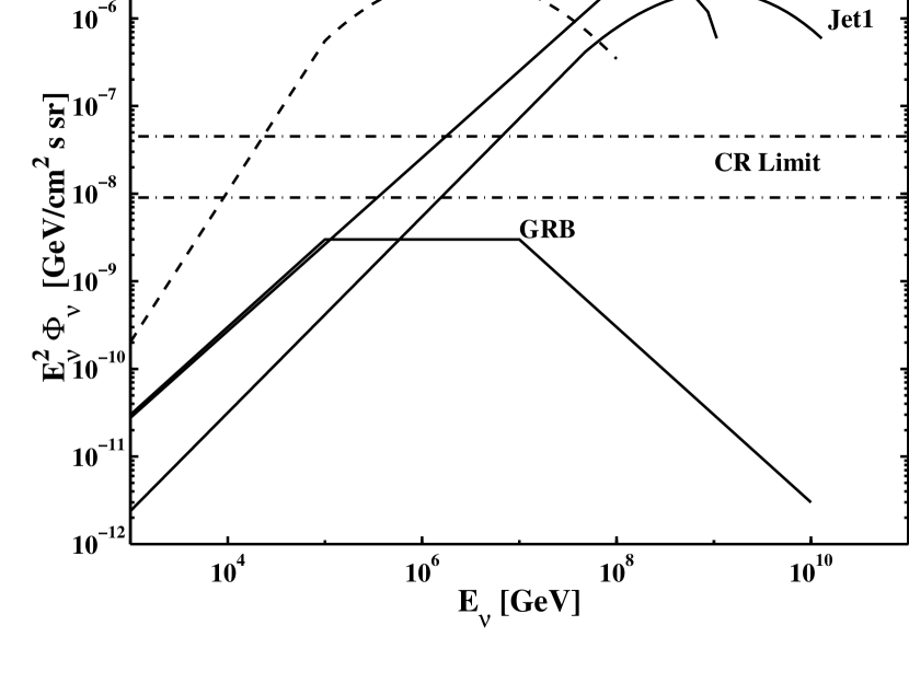
Figure 4: Differential muon neutrino flux weighted by the square of the muon neutrino energy versus muon neutrino energy. The WB limit is labeled as CR limit and compared to theoretical models. The Jet1 models refers to results from (Mannheim, 1995) and Jet2 from (Halzen and Zas, 1997). These models should be constrained by the WB limit. As they violate the limit, WB conclude that one of their assumptions must be wrong. The GRB model is a prediction for neutrinos from Gamma Ray Bursts (Waxman and Bahcall, 1999, 1997). The WB limit is also compared to a hidden source model (Stecker et al. 1991 and, 1992) for which the WB limit does not apply (see section 2.1.3). This model is at the level of the published AMANDA B-10 lower limit (Hill et al. 2001). Figure extracted from (Waxman and Bahcall, 1999).

It is important to note that the AGN sources are intermittent and that they might violate the WB limit in a temporary basis. However they should not do so when averaged over time.

2.2.2 Gamma-ray bursts

Energetic gamma-ray bursts (GRB) seem to be successfully explained by fireball models ((Piran, 1999) and references therein). Recent observations suggest that they originate in cosmological sources. Waxman and Bahcall (Waxman and Bahcall, 1997) propose that neutrinos are a consequence of these fireballs. They will be produced by photo-meson production between the fireball gamma-rays and accelerated protons. (Waxman and Bahcall, 1997, 1999) derive the energy spectrum and flux of high energy neutrinos created in this way. Their result is in agreement with (Rachen and Meszaros, 1998).

Figure 4 shows the predicted spectrum of high energy neutrinos from GRBs. This spectrum is consistent with the WB limit and the intensity over $2\pi$ sr coverage would be about 10 neutrino induced muons per year in a detector with $km^{2}$ incident area (Waxman and Bahcall, 1999). These neutrinos have the advantage of spatial and temporal coincidence with GRB photons which can be used as a tool to reduce the atmospheric neutrino background. The neutrinos produced from hadronic interaction may arrive on a time scale of about an hour after the photons in the model of simple acceleration (Waxman and Loeb, 2001).

2.2.3 Neutrinos from Galactic Point Sources

The neutrino flux from Sgr A East is analyzed as an example of a galactic point source. This is one of the dominant radio emitting structures at the Galactic Center and is a supernova remnant-like shell (Melia et al., 1998). It has been shown (Melia et al., 1998) that the highest energy component in the Sgr A East spectrum is compatible with a gamma-ray spectrum produced by pion decay. This energy spectrum fits the one from the galactic center source 2EG J1746-2852 measured by EGRET. The neutrino flux from Sgr A East was determined under the assumption that pion decay constitutes the gamma-ray source 2EG J1746-2852 (Crocker et al., 2000). Pions are produced in proton-proton collisions in shock regions and the maximum energy of the shocked protons is $\sim 5\times 10^{6}$ GeV. Neutrinos are produced from pion and muon decay. There is a ratio of about 67% muon like to 33% electron like neutrinos. We determine the sensitivity of a km² incident area to the largest neutrino flux, ie, the muon neutrino flux.

If neutrino oscillations occur as expected from Superkamiokande results (Fukuda et al, 1998) one should take this effect into consideration (Crocker et al., 2000, 2001). In this case, a portion of the muon neutrinos will most likely (Fukuda et al, 2000) become tau neutrinos. In this work we do not include oscillations and it represents an upper limit for muon neutrinos.

In Figure 2 we show the muon neutrino flux from Sgr A East as determined in (Crocker et al., 2000). The band represents the range between the best case scenario for which the proton energy spectrum will follow a power law with spectral index equal to -2.1 and the worst case scenario with spectral index equal to -2.4 Crocker et al. (2000). The cutoff is due to the maximum energy achieved by the proton. In section 3.4 we will determine the detectability of this flux of neutrinos.

Another galactic neutrino source might be supernova remnants (SNR). The CANGAROO collaboration has measured the gamma ray spectrum of a few of these sources (Tanimori et al., 1998; Muraishi et al, 2000). If the gammas were produced as a product of pion decays, neutrinos will also be produced. The neutrinos from SNR will however have a lower flux than the ones from Sgr A East and the cutoff energy will be at the TeV level instead of at the PeV level Crocker et al. (2001).

The brightest cosmic X-rays sources – the X-ray binaries – might also produce high energy neutrinos. Composed by compact objects such as black holes or neutron stars, they accrete matter from their companion stars. The accretion process might accelerate protons to high energies. The interaction of these protons with either the accreted matter or matter from companion stars will produce a neutrino flux. The neutrino flux from microquasars, which are Galactic jet sources associated with some classes of X-ray binaries has been determined in (Levinson and Waxman, 2001).

2.2.4 Neutrinos from the Sun

The high energy neutrino flux originating from cosmic ray interactions with matter in the Sun has been determined in (Ingelman and Thunman 1996b, ). Although it is higher than the atmospheric neutrino flux, the conclusion is that the absolute rate is low. Within the Sun’s solid angle, the neutrino energy spectrum will follow the atmospheric neutrino spectrum but is about 3 times higher. According to these authors the low rate precludes the Sun as a “standard” candle for neutrino telescopes and also limits neutrino oscillation searches. A detailed analysis of the influence of neutrino oscillations on the high energy neutrino event rates from the Sun can be found in (Hettlage et al., 2000).

2.3 Atmospheric Neutrino Fluxes

The atmospheric neutrino flux is the main background for neutrinos from astrophysical sources. As a parameterization of this background flux we use the derivation made by Volkova (Volkova, 1980) as described also in (Albuquerque and Smoot, 2001).

Volkova derives the atmospheric neutrino flux from the decay of light mesons ($K,\pi$) and muons and from the decay of short-lived particles (prompt decay) which mainly includes charm particles. The latter will only be significant at higher energies (above a PeV).

We compare this flux with that obtained by (Honda et al, 1995) and (Agrawal et al., 1996). The biggest difference between these calculations is of about 15% (see Figure 14 of ref. (Honda et al, 1995) and Figure 7 of ref. (Agrawal et al., 1996)). In the energy range of interest to our work, the discrepancy is less than 15% and the Volkova spectrum is underestimated in relation to these other spectra.

Since the atmospheric neutrino flux is irreducible, understanding the effect of its uncertainty is important. The uncertainties come from the primary cosmic ray flux measurement and from the inclusive cross section for proton – nucleon interactions. We assume the biggest discrepancy between the atmospheric flux calculations (15%) as the uncertainty in the magnitude of the atmospheric flux.

Since the uncertainty in the primary spectrum increases with energy there is also an uncertainty in the slope of the spectrum. At lower energy there are more data and the uncertainty is mainly due to instrumental efficiency and exposure factor. At higher energies the uncertainty is dominated by limited statistics. In general (Honda et al, 1995; Agrawal et al., 1996) the uncertainty in the spectrum slope is assumed to be about 10% below 3 GeV increasing to 20% at $3\times 10^{3}$ GeV and remaining constant from thereon. As discussed also in (Honda et al, 1995; Agrawal et al., 1996) the uncertainties in the interaction model at higher energies is estimated around 10%. Neutrino oscillations do not affect the atmospheric spectrum at the energies of interest here.

One can therefore estimate the overall uncertainty in the atmospheric neutrino flux as around 20%. We will show that this uncertainty does not affect significantly our results.

Although the atmospheric neutrino flux is always considered as a background for neutrino astrophysics, the fact that the flux at higher energies is not well determined by experiments, makes it an important measurement to be performed with neutrino telescopes. It has been suggested that the standard model neutrino cross section above $10^{8}$ GeV might be lower than expected (Dicus et al., 2001). Measuring the atmospheric neutrino flux at these energies can determine the neutrino – nucleon cross section (Kusenko and Weiler, 2001). It is important to note that these energies cannot be directly probed by accelerator experiments.

2.4 Summary of Fluxes

Figure 5 shows a summary of the expected fluxes arriving at the surface of the Earth from sources which produce high energy (around $10^{19}$ eV) cosmic rays. The atmospheric background dominates at low energy. Neutrinos from the center of the galaxy contribute a small excess to the atmospheric flux at energies above $10^{6}$ GeV, but are constrained by a smaller solid angle. They are not in the field of view of South Pole detectors, but are interesting for more equatorial detectors. Diffuse limits on astrophysical neutrinos are characterized by the WB limit. The WB limit is avoided by the MPR limits as they abandon the power-spectrum for optically thin limit and propose “hidden” source contributions for the optically thick limit. GZK fluxes are shown at the highest energies. The most promising flux to be measured is the one from GRBs since it allows reduction of the background through knowledge of arrival time and direction as well as the one from Sgr A East.

Detected event rates are smaller since the neutrino conversion into a muon and the efficiency of the detector have to be taken into account. Event rates and experimental sensitivity are considered in the next section.

A sensible design criteria for a neutrino detector is that it be sensitive to the highest known neutrino flux from astrophysical sources, namely five times below the WB limit. With such a sensitivity, backgrounds can be characterized and new diffuse fluxes discovered. Physics measurements of the new fluxes, namely brightness, energy spectrum and points on the sky, will require substantially more events.

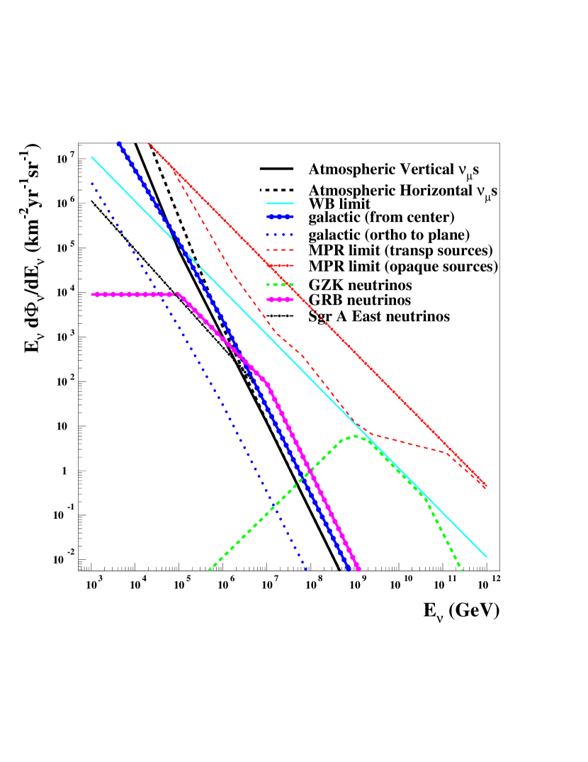
Figure 5: Differential muon neutrino fluxes weighted by neutrino energy summary containing (1) Atmospheric vertical (solid line) and horizontal (dashed) muon neutrino energy spectra based on (Volkova, 1980). The reason why these two fluxes overlap at high energies (above $10^{6}$ GeV) is that prompt decays (mainly from charm particles) dominate the atmospheric flux when compared to meson and muon decay at these energies.(2) WB (Waxman and Bahcall, 1999) limit (with evolution) for neutrino fluxes from astrophysical sources (large solid line). (3) Galactic neutrino flux (Ingelman and Thunman, 1996) from galactic center (dotted dashed line) and from direction orthogonal to the galactic plane (dotted). (4) MPR (Mannheim Protheroe and Rachen, 2001) limit for neutrino fluxes from sources transparent to nucleons (medium dashed line) and from sources opaque to nucleons (medium dotted dashed). (5) Estimate of GZK neutrinos (Engel and Stanev, 2001) (large dashed line). (6) Estimate of GRB neutrinos (Waxman and Bahcall, 1997) (large dot dashed line) (7) Estimate of Sgr A East neutrinos Crocker et al. (2000) assuming the best case scenario (see text) (medium dot dashed line).

3 Event Rates and Sensitivity

Neutrinos cannot be directly detected, because they do not deposit a significant amount of energy as they pass through matter. For a neutrino to be observed it must undergo an electro-weak interaction with another particle resulting in detectable secondaries. Since the neutrino interaction cross section is small, the probability of an interaction can be increased if large, dense targets are used, such as the Earth.

The neutrino nucleon cross section increases as a function of energy resulting in two effects. First, high energy neutrinos are more likely to interact within the detector volume. Second, the flux of neutrinos that reach the detector is attenuated at high energy because of neutrino interactions in the Earth. High energy muons travel many kilometers before stopping or decaying. The advantage of detecting muons is that the detector could be sensitive to neutrino interactions over a length equal to the muon range. Unfortunately, because high-energy muons lose energy rapidly and because at low energy there is a large atmospherically-produced neutrino background, this potential gain is reduced.

Convolution of the neutrino flux, conversion cross sections, muon range and deposited energy is the subject of the next sections.

3.1 Neutrino Interactions

The flux of leptons converted from the incident neutrino flux is

$$\phi_{lepton}=\phi_{\nu}P(\nu\rightarrow lepton)$$ (4)

where $P(\nu\rightarrow lepton)$ is the probability that a neutrino suffers an interaction and produces a lepton. This probability is given by

$$P_{I}=P(\nu\rightarrow lepton)=\int_{0}^{path}{\rm n}\sigma(\nu\rightarrow lepton)dx$$ (5)

where ${\rm n}$ is the nucleon number density and $\sigma$ is the neutrino nucleon cross section and the path is the distance the neutrino traveled. In the following, we abbreviate the notation: $P_{\rm I}=n\sigma_{\nu}L$ where $L$ is the neutrino path.

The deep inelastic neutrino cross sections, $\sigma_{\nu}$ are determined using CTEQ4-DIS parton distribution functions as described in (Gandhi et al., 1998). In the case of muon neutrinos, the interaction probability is dominated by the charge current (CC) cross section, but there is also some degradation of neutrino energy by the neutral current (NC) cross section.

Neutrino fluxes will suffer attenuation as they pass through the Earth. The differential flux is given by

$$\frac{d\phi_{\nu}}{dx}=-n\sigma_{\nu}\phi_{\nu}$$ (6)

where $x$ is the distance traveled by the neutrino. Integrating over the path length traversed by the neutrino, we find

$$\phi_{\nu}=\phi_{\nu 0}e^{-\int n\sigma(\nu)dx}=\phi_{\nu 0}P_{S}$$ (7)

where $\phi_{\nu 0}$ is the flux at the earth’s surface, $P_{S}$ is the survival probability and the argument of the exponential term is $P_{I}$ integrated over all cross sections that make the neutrino cease to exist.

Figure 6 shows the muon neutrino survival probability at a point on the surface of the earth for a variety of neutrino energies as a function of the cosine of the earth angle, $\theta_{Z}$ . The number density (see Equation 5) is determined by an integration of the earth density profile which is taken from (Gandhi et al., 1996; Dziewonski, 1989). The upper lines are the probability using only CC interactions. The lower lines include both CC and NC interactions. It shows that the NC interaction will decrease the lepton flux by about 10%. At high energy, the steep cut-off results in as much as a 20% decrease. The NC interaction does not actually remove the neutrino from the flux, but degrades its energy. We include it in our analysis to be conservative, and treat the CC-only case as an upper bound to the systematic uncertainty.

From Figure 6 one can see that the survival probability becomes quite small for high energy neutrinos due to significant attenuation. At low energies, the attenuation is negligible, but it begins to contribute above about 10 TeV. The Earth becomes essentially opaque to neutrinos at energies of above a PeV (Gandhi et al., 1998).

The effect of the dense Earth core can be seen near $\cos{\theta_{Z}}$ of 0.8. Neutrinos that travel close to the Earth axis will go through most of the Earth core and therefore increase their probability of interaction. There is also evidence of a thin crust at small $\cos{\theta_{Z}}$ where neutrinos only pass through the crust.

Figure 6: Survival probability for neutrinos and anti-neutrinos transversing the Earth as a function of $\cos(\theta_{Z})$. The horizon is at 0, and a path through the center of the earth is at 1. The upper lines include only CC interactions, the lower lines include both CC and NC interactions. Differences due to NC interactions have a maximum effect at high energy where the distributions drop sharply.

The flux of muons interacting in a detector volume is given by

$$\phi_{lepton}=\phi_{\nu 0}\times P_{S}\times P_{I}$$ (8)

where the incident flux, $\phi_{\nu 0}$, is the flux in Figure 5 and $P_{I}$ is now integrated over the neutrino path through the detector.

3.2 Muon Fluxes

Muons will propagate, losing energy until they eventually come to rest and decay or undergo a nuclear reaction. The mean energy loss is given by

$$\frac{dE_{\mu}}{dx}=a+bE_{\mu}$$ (9)

where asymptotically $a=2\times 10^{-3}{\rm GeVcm^{2}/g}$ and $b=4\times 10^{-6}{\rm cm^{2}/g}$ (Groom et al. 2000a, ) are respectively ionization and radiation loss parameters.

Approximating the parameters $a(E_{\mu})$ and $b(E_{\mu})$ as constants, simple integration over the muon path yields the muon range, $R_{\mu}$.

$$R_{\mu}=\frac{1}{b}\ln\left(1+\frac{b}{a}E_{0}\right)$$ (10)

where $E_{0}$ is the muon initial energy. Below the critical energy ionization losses dominate and the muon range is well described by the average energy loss. At high energies where radiative processes dominate, large fluctuations develop and a stochastic approach is needed. The mean muon range is shorter than Equation 10 would suggest. Lipari and Stanev (Lipari and Stanev, 1991) developed a Monte Carlo with the purpose of taking these fluctuations into account. We use their Monte Carlo to determine the muon range. This approach also accounts for the energy dependence of the energy loss parameters $a$ and $b$.

We now determine the upgoing muon rate in an idealized detector located 1.5 km below the surface of the earth with a detector path length of 1 km and a km² incident area for all incident angles. Two muon rates are relevant, those where the muon is produced inside the detector ($P_{I}$ integrated over 1 km) and those where the muon originates outside the detector and ranges into the detector ($P_{I}$ integrated over the muon range). Figure 7 shows the rate of upgoing muons plus anti-muons weighted by neutrino energy versus neutrino energy for the WB limit, the MPR limit, GRB flux, GZK flux, and for atmospheric neutrinos. Only muons with more than 100 GeV are included. These results are in good agreement with (Gaisser, 2000). The lower curve is the flux of muons plus anti-muons that start outside the detector volume and range into it. The upper curve includes the flux of muons and anti-muons that start in the detector volume. Except for very low energies, the dominant flux is from muons that range into the detector.

Muons associated with the galaxy are not isotropic. We make estimates for a detector at a Mediterranean latitude of +35 degrees corresponding to a expanded version of the ANTARES or NESTOR detector. A North Pole detector would see a rate 1.6 times higher. The galactic center is above the horizon at the South Pole where the atmospheric muon background is too high. Figure 7 shows the rate of neutrinos from 75 square degrees in the galactic plane, centered on the galactic center. The rate is much smaller than the Atmospheric neutrinos in the same solid angle. We conclude, therefore that Galactic neutrinos will not be detectable.

We also determine the muon rate for Sgr A East at a latitude of 35 degrees. Two rates are shown in Figure 7 corresponding to hard and soft proton spectra with a cut-off at $5\times 10^{6}$ GeV (see section 2.2.3). Background neutrinos from the galaxy in 1 square degree surrounding Sgr A East are about 75 times smaller than the rate shown in the figure. For point sources such as GRB and Sgr A East, the primary background of atmospheric neutrinos is reduced in 1 square degree by a factor of about $5\times 10^{-5}$ again leaving a nearly background-free source detection.

Muon rates are substantially lower than the neutrino rates shown earlier. The line on Figure 7 shows where 1 event/year is expected for each half decade in energy. The GZK flux peaks at $10^{9}$ GeV, just below the WB limit. About 0.17 muon per year is expected from the GZK flux.

For all but the atmospheric flux, equal numbers of neutrinos and anti-neutrinos are expected. Atmospheric neutrinos exceed anti-neutrinos by a factor of 2.5 at 1 TeV (Agrawal et al., 1996). By about 100 TeV, however, the neutrino and anti-neutrino cross sections become equal. Across the whole spectrum, the uncertainty due to muon/anti-muon composition can be neglected since it is smaller than the theoretical uncertainty of $\pm 20$%.

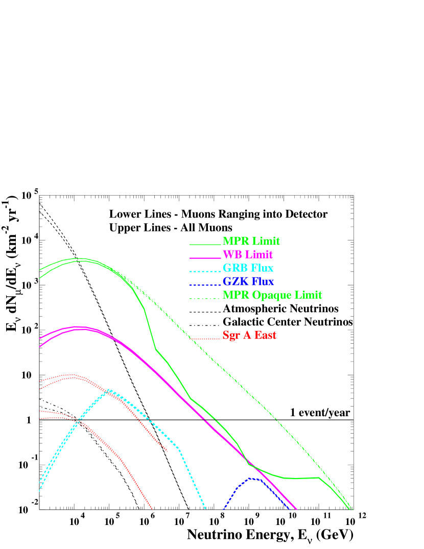
Figure 7: Differential upgoing muon and anti-muon rate weighted by neutrino energy as a function of neutrino energy. Most muons range into the detector although the fraction starting inside increases at low energy. The horizontal line shows where 1 event/year is expected for each half decade in energy.

Since the neutrino energy is not measured by the detector, but rather the muon energy is estimated by energy deposition in the detector, the results are better shown as a function of the muon energy estimation. The latter can be achieved in three steps: (1) first the flux as a function of the muon energy, (2) as a function of the muon energy at the detector, and (3) finally flux as a function of the energy deposition in the detector. The muon flux as a function of muon energy is given by

$$\phi_{\mu}=\int_{0}^{\infty}\frac{d}{dE_{\mu}}(\frac{d\phi_{\nu}}{dE_{\nu}})dE_{\nu}$$ (11)

The average energy loss in a CC interaction, $y=(1-E_{\mu}/E_{\nu})$, for neutrinos energies between 10 GeV and 100 GeV is 0.48 gradually decreasing to about 0.2 at high energies (Gandhi et al., 1996). At high energy, the muon gets about 80% of the neutrino energy.

A stronger effect is noticed if we determine the flux as a function of the muon energy as it enters the detector. A very high-energy neutrino will make a very high-energy muon that travels many kilometers losing energy as it goes. If the track starts at random distance from the detector, the measured energy will be distributed nearly uniformly between the initial energy and zero. A high-energy muon will lose on average 1-1/e of its energy when traversing between 2.4 and 3 km of ice. About each 2.7 km of ice traversed will move the muon down a natural logarithmic energy interval of muon energy at the detector. We use the Lipari-Stanev Monte-Carlo (Lipari and Stanev, 1991) to determine the muon range and the energy deposited in 100 m steps including fluctuations from radiative processes. A random spot is chosen along the track to represent the point it enters the detector. Figure 8 shows the differential muon plus anti-muon rate weighted by muon energy resulting from neutrino interactions as a function of the muon energy as it enters the detector.

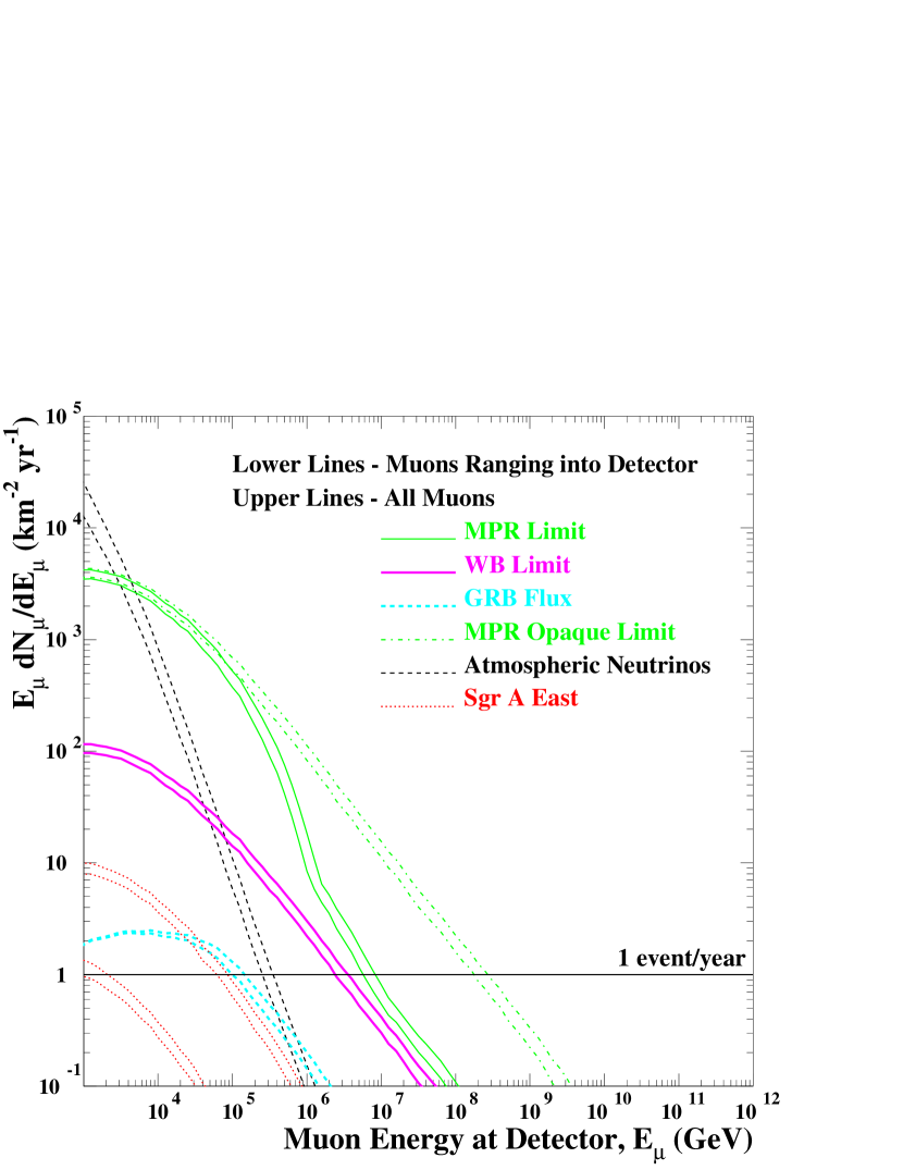
Figure 8: Differential upgoing muon and anti-muon rate weighted by muon energy as a function of the muon energy when it enters the detector. The measured energy of muons that range into the detector is less than the initial energy. Muons that start inside the detector make up about 30% of the flux at high energy.

The atmospheric neutrino flux is a major background over most of the energy range where events can be measured in a ${\rm km^{2}}$ per year. To detect the high-energy signals, good energy resolution is needed. For point sources, the muon energy is used as a cut parameter to optimize signal to background. For the diffuse flux, the resolution is needed to deconvolve the spectrum back to the neutrino energy. Where signals are not detected, a cut on muon energy is needed to set upper limits.

3.3 Muon Energy Resolution

Muon energies below about 100 GeV are measured by their path length. At higher energies, the path lengths become too long and the amount of Cherenkov radiation from the track is used. The total Cherenkov radiation is nearly proportional to the total energy deposition in the detector volume. Figure 9 shows the deposited energy in MeV/m for 100, 500 and 1000 meter track lengths at a variety of muon energies. The distribution is essentially a Gaussian with a long tail to larger energy deposition due to the stochastic nature of the energy loss processes. The energy loss includes (Lipari and Stanev, 1991) the usual ionization and knock-on electron processes important at lower energies and additional processes important at higher energies including pair production ($\propto\Delta E^{-\beta}$, $\beta$ varying from 1 to 3 as $\Delta E$ increases) Groom et al. (2001), bremsstrahlung ($\propto\Delta E^{-1}$), and photonuclear (roughly $\propto\Delta E^{-1.1}$), all with a cut off at the total energy of the muon. These processes are responsible for the energy dependent portion of $dE/dx$. The numerous lower energy pairs (plus ionization) produce the Gaussian-peaked shape for most energy losses. The bremsstrahlung and photonuclear processes and the rarer high-energy pairs produce a significant tail of much larger energy depositions. If the most probable (or mean) energy deposition is used as a measure of the muon energy, a significant number of the much more abundant lower energy muons will be reconstructed as high energy muons. As a result a significant number of the abundant atmospheric muons would be reconstructed as much higher energy muons. Longer sampling path lengths have a more truncated tail because there is a cut off where the muon is completely stopped. The deposited energy can not exceed the muon energy. A clear statistical relationship exists between detected and true muon energy.

Figure 9: Energy deposited in MeV/m for 100m, 500m, and 1 km muon paths. Notice there is a strong dependence in the deposited energy on the true muon energy until the muon energy drops below about 100 GeV.

An ideal detector could measure the deposited energy perfectly. If an ideal detector made many measurements with independent 100 meter samples, then events that fluctuated early could be removed at the expense of efficiency and the true muon energy could be measured using the samples up to the first large fluctuation. The Frejus detector (Rhode et al, 1996) being a sampling calorimeter determined the muon energy based on fluctuations in energy deposition. The large scale of more recent neutrino detectors makes independent sampling unrealistic. In an open geometry, such as Cherenkov detectors, the samples can not be cleanly separated with opaque barriers. Long path lengths are an advantage because they minimize the sensitivity to the long tails in the energy resolution. Under sampling can reduce the advantage of long path lengths, however if the detector is only able to measure portions of the energy deposition. Figure 10 shows the differential upgoing muon rate weighted by the energy deposited in the detector as a function of energy deposited in the detector as radiation in a 500 meter track.

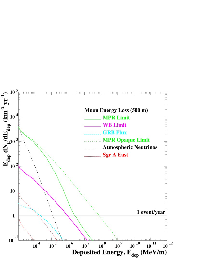
Figure 10: Differential upgoing muon and anti-muon rate weighted by energy deposited in the detector as a function of the energy deposited in the detector.

Figure 11 is included to show the main systematic effects on the spectrum. High energy muons are most sensitive to the NC effect on survival probability. The shape of the atmospheric background depends more significantly on the length of the track. In addition to the systematics shown on the plot, there is about 20% theoretical uncertainty in the predicted atmospheric flux (see section 2.3).

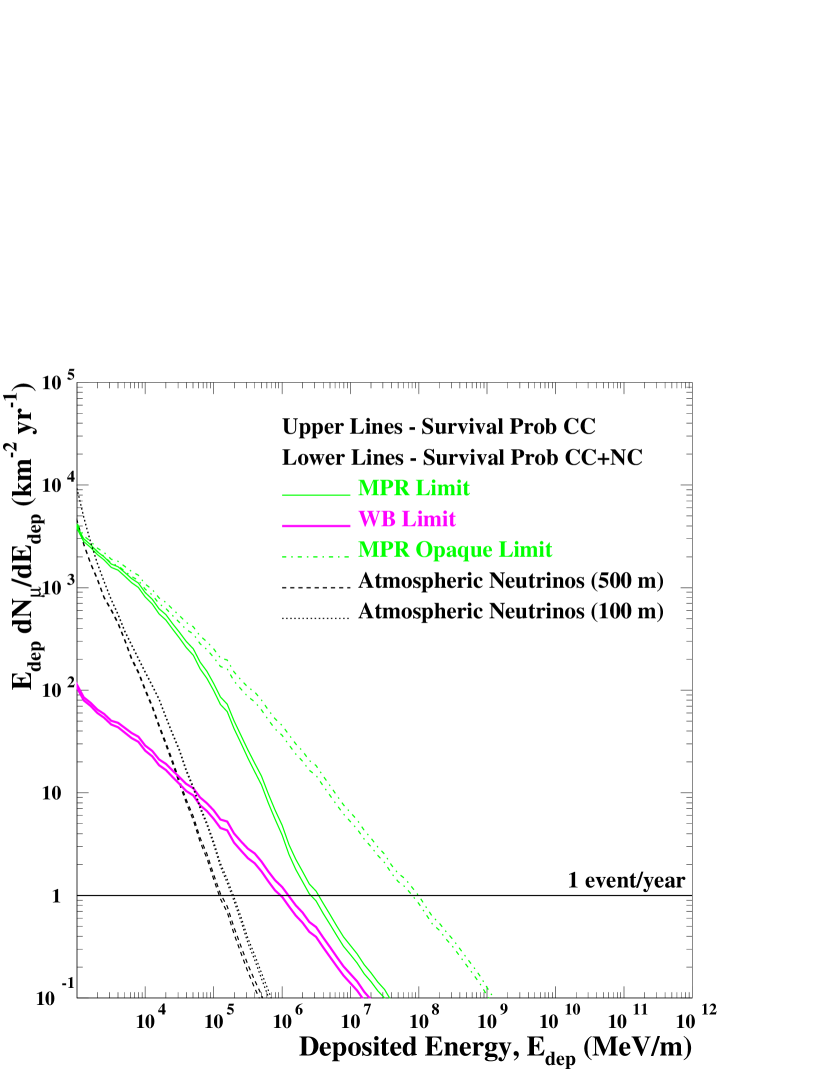
Figure 11: The spectral dependence on survival probability and path length. Neutral currents (NC) primarily affect the overall normalization of the hard spectra. The spectrum dependence on path-length is shown for the steep atmospheric background where the resolution tails become important. For 100 m paths there is a kink in the distribution. Without tails in the resolution, such a change in slope would signal the discovery of a new source of neutrinos. We use the 500 m resolution for our ideal detector and add the actual path length in Section 4 for real detectors.

3.4 Sensitivity of an Ideal km² Detector to Astrophysical Sources

Event rates above a cut where signal and background are equal are listed in Table 1. Also included are rates for two other possible energy cuts: the energy where no background events are expected (atmospheric $<$ 0.1 event), and the energy where 1 background event is expected. Uncertainties in the rates come from several sources. There is a theoretical uncertainty on the atmospheric background of $\pm$20%. The NC contribution to the survival probability is +10%. Finally, the difference between Lipari-Stanev and a smooth parameterization of the energy deposition adds $\pm 10\%$ for 500 meter tracks and $\pm 50\%$ for 100 meter tracks. The total uncertainties in the event rates quoted (500 m tracks) are: +14%, -10% for signals and +24%, -22% for the atmospheric flux.

Muon Source	events	events	energy (Mev/m)	events
	E$>10^{5.5}$ MeV/m	E$>10^{4.95}$ MeV/m	S/B=1	E$>$S/B=1
Atmospheric Neutrinos	0.11	1
WB Opt Thin Limit	3.0	7.8	$10^{4.3}$	23.8
MPR Opt Thin Limit	15.5	90.0	$10^{2.8}$	7500.0
MPR Opaque Limit	112.0	300.0	$10^{2.9}$	7050.0
MPR Source ($10^{3}GeV)$	10-12	10-7
MPR Source ($10^{4}GeV)$	0.0003	0.31	$10^{3.0}$	2500.0
MPR Source ($10^{5}GeV)$	3.4	60.0	$10^{2.9}$	4000.0
MPR Source ($10^{6}GeV)$	5.8	21.0	$10^{3.9}$	76.0
MPR Source ($10^{7}GeV)$	2.5	4.5	$10^{4.5}$	6.4
MPR Source ($10^{8}GeV)$	0.9	1.3	$10^{4.9}$	1.4
MPR Source ($10^{11}GeV)$	0.1	0.1

Table 1: Event rates for 500 meter long muon tracks in an ideal km² detector per year. The background is composed of atmospheric neutrinos. Background-free limits can be estimated for deposited energy $>10^{5.5}$ MeV/m. A single background event is expected for energy $>10^{4.95}$ MeV/m. Finally, the energy and rates where the signal equals background (S/B=1) are listed. Uncertainties in event rates are +24%, -22% for atmospheric background and +14%, -10% for the other signals.

Also included in the table are a series of sources consistent with the MPR optically thin limit. Since this limit is not a power law, it is a composite of sources at each energy. The maximum power-law spectrum consistent at all energies is the WB limit. Figure 12 shows the neutrino flux for these made-up sources. We generously give them a E^-1 isotropic spectrum, cut-off by a gaussian shape with means varying from $10^{3.0}$ to $10^{11.5}$ GeV, and widths of $\sigma=0.3$. Their normalization varies between the MPR thin limit and WB limit. Figure 13 shows the differential upgoing muon rate weighted by the energy deposited in the detector for these sources as a function of deposited energy in the detector. From the numbers tabulated in Table 1 it is clear that the a km² detector will be sensitive to neutrino fluxes with incident energies between $10^{5}$ and $10^{7}$ GeV. Higher fluxes have been ruled out by the cosmic ray spectrum and lower fluxes are buried below the atmospheric background.

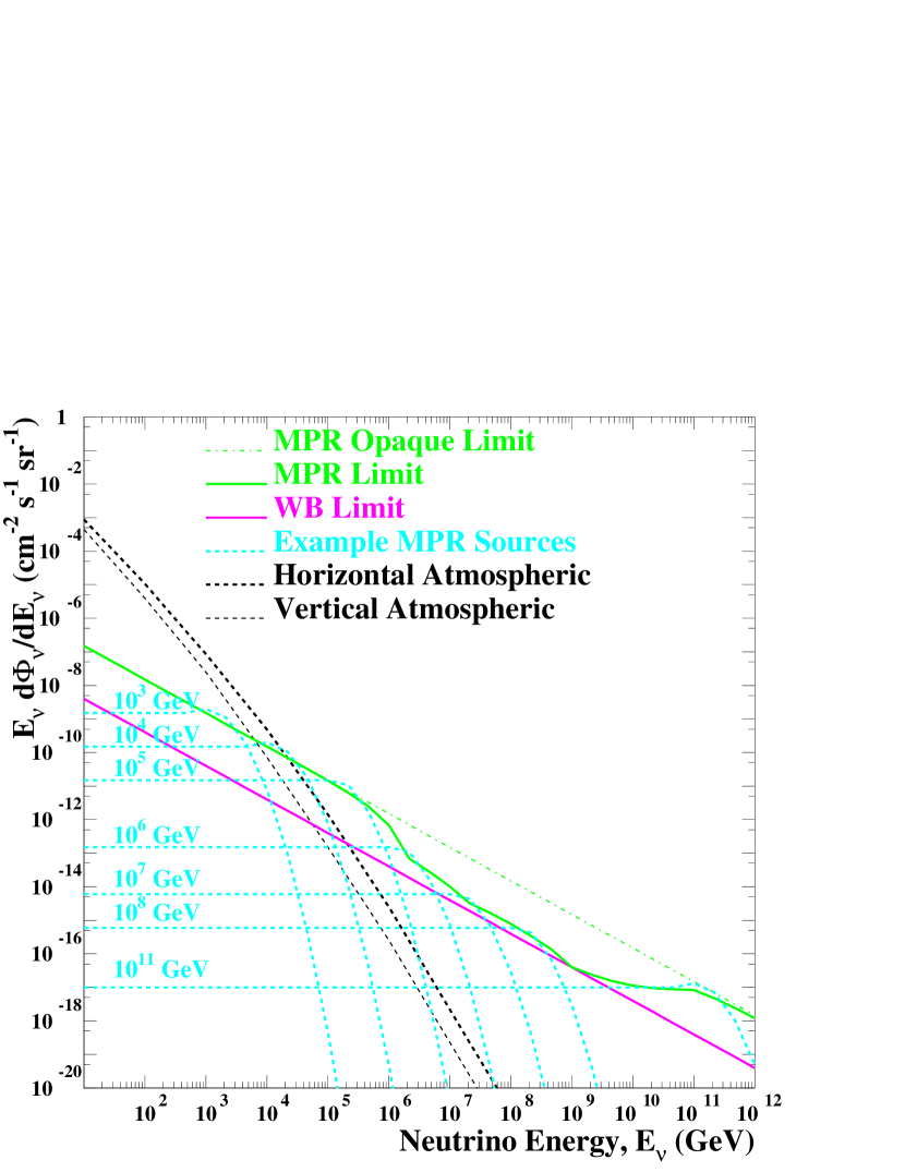
Figure 12: Possible sources making up the MPR flux. Sources are E^-1 spectra cut-off by a gaussian of width 0.3. Amplitudes GeV/(cm² s sr) (cut-off energy(GeV)) $1.5\times 10^{-6}$ (10³), $1.5\times 10^{-6}$ (10⁴), $1.5\times 10^{-6}$ (10⁵), $1.5\times 10^{-7}$ (10⁶), $6.0\times 10^{-8}$ (10⁷), $6.0\times 10^{-8}$ (10⁸), and $1.0\times 10^{-6}$ (10¹¹).

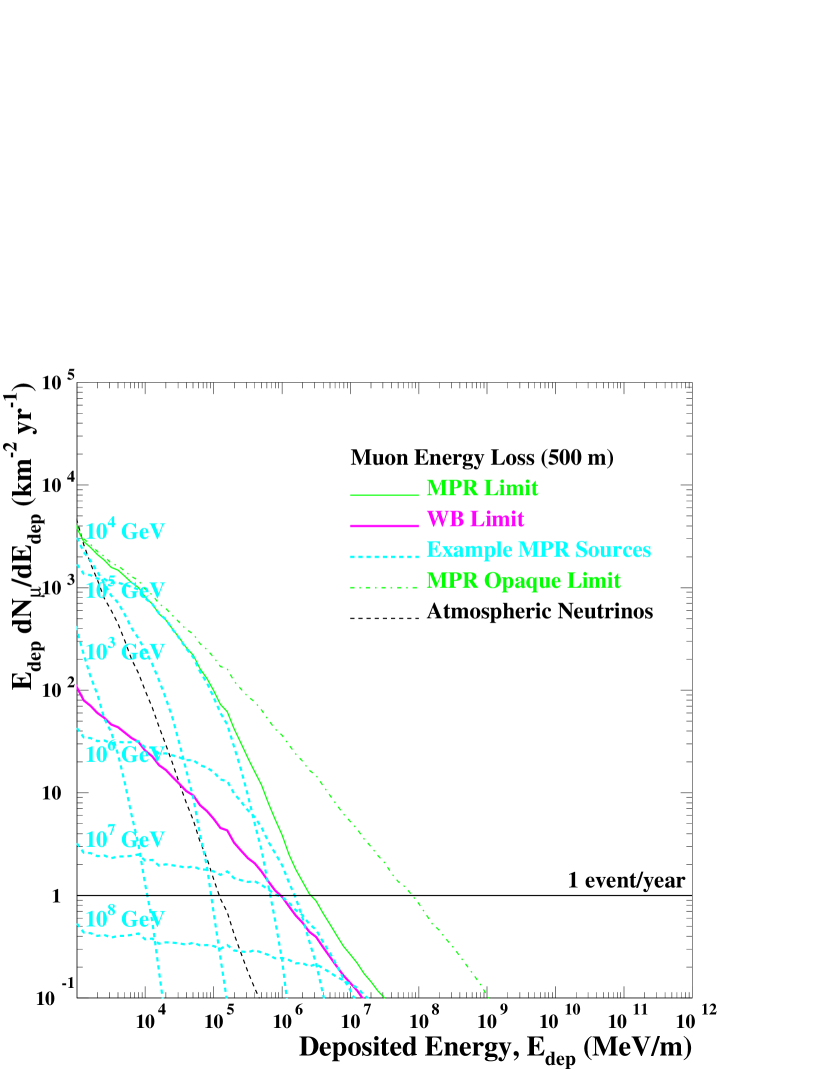
Figure 13: Differential upgoing muon rate weighted by deposited energy as a function of energy deposited in the detector for a series of example sources that could make up the MPR flux.

In the absence of signal events, flux limits can be set Groom et al. 2000b ; Feldman and Cousins (1998) based on the number of events observed, $n_{obs}$, by an experiment and knowledge of the mean background expected, $b$. The poisson probability that an observation is consistent with a mean signal, $s$ is given by

$$P(n_{obs}|s)=(s+b)^{n_{obs}}exp[-(s+b)]/n_{obs}!$$ (12)

Integrating this over all signals up to a confidence level, $CL$, gives the standard confidence belt, $s_{CL}(n_{obs},b)$. Feldman and Cousins suggest that this belt be modified to avoid flip-flopping between one and two-sided intervals based on the experiment performed. Here we choose the simpler approach of always using a one-sided limit. The Feldman and Cousins approach leads to $\sim 10$% weaker limits for very low statistics experiments. The experimental flux limit is defined as

$$\Phi_{limit}=\phi_{s0}\times\frac{s_{CL}(n_{obs},b)}{s}.$$ (13)

where $\phi_{s0}$ is the theoretical neutrino signal flux. Before the experiment is performed, there are no observed events. It is still interesting to determine the average $<s_{CL}(n_{obs},b)>$ of a collection of proposed experiments having only background events. (Hill et al., 2001)

$$<s_{CL}(n_{obs},b)>=\sum_{n_{obs}=0}^{\infty}s_{CL}(n_{obs},b)P(n_{obs}|b)$$ (14)

We define the average limit that a detector can place on signal fluxes to be the sensitivity of the detector, $\Phi_{sensitivity}$.

$$\Phi_{sensitivity}=\phi_{s0}\times\frac{<s_{CL}(n_{obs},b)>}{s}.$$ (15)

The ratio $\phi_{s0}/s$ is the detection transfer function. The magnitude of the signal flux cancels in the ratio leaving only the sensitivity to the spectral shape.

3.4.1 Diffuse Limits

Table 2 shows the sensitivity (95% CL) of an ideal detector of km² incident area to neutrino fluxes and various spectral shapes as suggested in (Mannheim Protheroe and Rachen, 2001). Included in these estimates are systematic uncertainties in the background normalization.

Systematic uncertainties affecting the background and signal bound our knowledge of the measurement. For example, an experiment that expects 1000 background events can easily discover a signal with 100 events, even with poisson sampling statistics. But this same experiment with a 10% uncertainty in the background is barely sensitive to a signal with 200 events. The limits quoted in Table 2 include Poisson statistics as described above, but limit the sensitive region to where the signal is larger than the 2 $\sigma$ uncertainty on the background.

Muon Source Flux	Optimized	Atmospheric	Signal	Original	km2 Sensitivity
	Energy Cut	Background, $b$	$s$	Amplitude	GeV/cm2 s sr
	(MeV/m)	(events)	(events)	GeV/cm2 s sr	(95% CL)
WB Opt Thin Limit	$10^{4.3}$	16.1	23.8	$4.0\times 10^{-8}E^{-}2$	$1.3\times 10^{-8}$
MPR Opt Thin Limit	$10^{4.3}$	16.1	487.	varies	$\times 0.016$
MPR Opaque Limit	$10^{4.3}$	16.1	893.	$1.5\times 10^{-6}E^{-}2$	$1.3\times 10^{-8}$
MPR Source (104 GeV)	$10^{4.3}$	16.1	36.4	$1.5\times 10^{-6}$	$2.1\times 10^{-7}$
MPR Source (105 GeV)	$10^{4.3}$	16.1	448.	$1.5\times 10^{-6}$	$2.6\times 10^{-8}$
MPR Source (106 GeV)	$10^{4.6}$	4.47	36.1	$1.5\times 10^{-7}$	$2.2\times 10^{-8}$
MPR Source (107 GeV)	$10^{5.0}$	0.83	4.31	$6.0\times 10^{-8}$	$4.4\times 10^{-8}$
MPR Source (108 GeV)	$10^{5.3}$	0.24	1.07	$6.0\times 10^{-8}$	$1.4\times 10^{-7}$

Table 2: Sensitivity of a km² detector to fluxes with a variety of spectral shapes based on 1 year statistics.

We find that a detector with km² incident area will be sensitive to a spectral flux three times smaller than the WB limit. From the MPR sources, we can see that the limit is most sensitive to neutrinos of  1 PeV. Neutrinos between $10^{5}$ and $10^{7}$ contribute most to the signal rate.

3.4.2 Point Source Detection - GRB

One easy way to reduce the background in these experiments is to narrow the search bin from half the sky to the characteristic size of the detected angular resolution. The intrinsic resolution of a muon’s direction with respect to the neutrino is about 1 square degree. In this way, we can divide half the sky into 20,628 one degree square patches of sky. There are two kinds of searches. The first involves looking for neutrinos from sources that are known to exist. The second involves looking for sources anywhere on the sky.

The GRB flux is a case where both the time and location of the burst is known apriori. In this case, we take all known bursts and search in one degree bins, coincident in time. The integrated GRB signal from Figure 10 is 15 events per year. The number of GRB detected in a year depends on the sensitivity of experiments like BATSE or MILAGRO. Based on expectations of these detectors, we estimate somewhere in the range of $10^{2}-10^{3}$ GRBs per year. Assuming that all 15 muons above were produced in some fraction of these GRBs, we find that the expected background in all GRB events is 0.015 muons. A $5\sigma$ discovery can be made even if the GRB flux is reduced by a factor of 5.

Somewhat surprising is the robustness of this result to variations in the number of detected GRBs and the time-scale of the event. Depending on the number of GRBs detected by other experiments, the background can change by an order of magnitude. Similarly, if the neutrinos arrive over a 24 hour period instead of a 1 second pulse (used in the above calculation – see section 2.2.2) then the background is 86000 times larger. In this case, the best limit comes from applying an energy cut at $10^{2.4}$ MeV/m which leaves only 0.012 background events and 13 GRB neutrino induced muons. If this energy cut is not possible, then the background is too large, and there is no way to find GRB muons that arrive on a long time scale.

3.4.3 Point Source Detection - Sgr A East

Sgr A East is an example of a bright galactic source. It is known to vary in brightness, but on a time-scale of months so that it is reasonable to expect measurements to integrate the neutrino signal over a full year. We estimate that the Sgr A East rate is between 0 and 40 neutrino induced muons per year in an ideal km² detector at a latitude of +35 degrees. The Atmospheric Neutrino background is reduced by knowing the location of the source. The best $5\sigma$ limit comes from applying an energy cut at $10^{2.4}$ MeV/m which leaves only 4 background events and 33 neutrino induced muons from Sgr A East with the hardest hypothesized proton spectrum. Such a detector (equivalent to a km scale Mediterranean-based detector) will be sensitive to a source even half as bright. The softest spectrum is about ten times dimmer and would not be detectable.

3.4.4 Point Source Detection - AGN

Another type of point-source search involves looking for sources without prior knowledge of location or time. Here we reduce the up-going atmospheric neutrino background by 20,628 search bins on the sky. The signal is also divided among an unknown number of sources.

There is an art to choosing bins on the sky. If the bins are chosen before the experiment is performed, then sources will not fall in just one bin, and the search is not efficient. If sliding windows are used to find spots with the largest number of events, then the search is biased to the locations where the background has clustered. A poor-man’s alternative is to consider a fixed array of search bins, but to perform 100 searches with each shifted by 1/10th of a degree in azimuth or zenith from the previous search. This is a close approximation to 100 independent searches of the sky. The signal will be 90% contained in at least one search, and can therefore be approximated by the true signal, ignoring the cases where the signal is partially contained in a different search. The effect is that instead of performing 20,628 experiments for each spot on the sky, we perform 2,062,800 experiments. To avoid mistaking a background fluctuation for signal, we calculate $6\sigma$ limits which will only be wrong one time out of 5 million.

If the entire isotropic diffuse flux is produced entirely from one point source (within a single degree-square bin) then an ideal km² detector will be sensitive to a flux $1.4\times 10^{-9}$E^-2 GeV/(cm² sr s) at $6\sigma$. This is 28 times lower than the WB limit. Since the rate of neutrinos is expected to be about 5 times lower than the limit, we conclude that this rate is expected and easily detected. If, however, the flux is divided between 10 bright sources, then we will only be sensitive to a flux 2.8 times lower than WB, and a point source discovery would indicate new physics. This limit scales linearly with the number of sources that contribute to the flux; so, for example, $10^{3}$ sources are the maximum that may be detected by an ideal km² detector because more would violate the MPR Opaque Limit.

The diffuse limits have been treated as isotropic. From Figure 6, one can see that the diffuse flux ($10^{5}-10^{7}$ GeV) is biased toward the horizon. Astronomy with neutrinos relies on the flux being divided among a handful of bright point sources located within a few tens of degrees of the horizon.

4 Sensitivity of Proposed and Existing Detectors

The above calculations used an ideal geometry of a detector with km² incident area and 500 meters long for all zenith angles. We now include the geometry of proposed detectors to determine their acceptance. Combining the irreducible physics effects with the detector acceptance allows us to determine the best possible limit for such detectors.

Not included are the effects of specific detector designs which can only degrade the sensitivities. In real life detectors tend to be cylinders or spheres sunk into deep water, ice or caves. The interaction probability of the rock below or surrounding the detectors and the passive detecting medium of the instrument have to be considered. Particularly important effects which are not addressed in this paper are the number of sampling elements, the sensitivity of the detecting elements, the uniformity of the detecting medium, and the conversion of “deposited radiation” into a measurable light spectrum.

Figure 14 shows the geometrical profile of IceCube, AMANDA-II, ANTARES, NESTOR, and AMANDA-B10 as a function of zenith angle. Figure  15 shows the mean detector path length and efficiency assuming a reasonable minimum path length. IceCube is by far the largest, with essentially km² acceptance. AMANDA-II, ANTARES, and NESTOR are all of similar size and and AMANDA-B10 is the smallest.

Table 3 lists the sensitivities of these detectors to an E^-2 flux of high-energy neutrinos. These estimates include the effects of neutrino attenuation in the earth, muon transport, and fluctuations in energy deposition. For IceCube, a 300 m minimum track is required to reduce the systematic effects of the long tails in the resolution. For the others, a 100 m minimum track is required. For the smaller detectors, the irreducible systematic uncertainty is quite important. For IceCube, we use +24% for the atmospheric background systematic uncertainty, and for the others we use +50% (see section 3.4). Limits without systematics are 10% better for IceCube, and 30% better for the smaller detectors.

	Optimized		Atmospheric		WB Signal		Sensitivity
Detector	Energy Cut		Background, $b$		$s$
	(MeV/m)		(events)		(events)		(GeV/cm2 s sr)
CL	$90\%$	$95\%$	$90\%$	$95\%$	$90\%$	$95\%$	$90\%$	$95\%$
IceCube	$10^{4.3}$	$10^{4.2}$	9.1	13.9	19.1	22.7	$1.1\times 10^{-8}$E-2	$1.4\times 10^{-8}$E-2
AMANDA-II	$10^{4.1}$	$10^{4.0}$	2.9	4.3	2.2	2.6	$6.5\times 10^{-8}$E-2	$8.0\times 10^{-8}$E-2
ANTARES	$10^{4.0}$	$10^{3.9}$	2.8	4.1	1.6	1.9	$8.7\times 10^{-8}$E-2	$1.1\times 10^{-7}$E-2
NESTOR	$10^{4.1}$	$10^{3.9}$	2.7	5.8	2.0	2.8	$7.0\times 10^{-8}$E-2	$8.2\times 10^{-8}$E-2
AMANDA-B10	$10^{3.9}$	$10^{3.7}$	2.8	5.4	1.2	1.7	$1.2\times 10^{-7}$E-2	$1.3\times 10^{-7}$E-2

Table 3: Sensitivity of existing and proposed detectors to fluxes with E${}_{\nu}^{-2}$ spectral shapes based on 1 year statistics.

We state in section 2.4 that to ensure the discovery of neutrinos from astrophysical sources one needs a detector sensitive to about one fifth of the WB flux. We find that current and future detectors are at most sensitive to one third of the WB flux. IceCube will reach a sensitivity of one fifth the WB flux after 2-3 years of 100% efficient operation. To characterize the source luminosity or energetics would require additional factors of 10-100 in rate.

Figure 14: Geometrical dependence of the IceCube, ANTARES, NESTOR and AMANDA detectors as a function of zenith angle. Dimensions are for a cylinder of (depth, height, diameter) in meters: IceCube (1850, 900, 1000), AMANDA-II (1740, 500, 200), ANTARES (2250, 300, 200), NESTOR (3400, 450, 200), AMANDA-B10 (1740, 500, 120).

Figure 15: Geometrical efficiency for tracks longer than either 100 or 300 meters as a function of zenith angle.

5 Conclusions

We have summarized the muon neutrino plus muon anti-neutrino fluxes from astrophysical sources. We include fluxes predicted by models within the particle physics standard model and do not include the ones predicted by exotic models. In this way the muon neutrino flux is constrained by the Waxman and Bahcall limit (WB) (Waxman and Bahcall, 1999) for energies above $10^{6}$ GeV. The “thin source” (see 2.1.2) limit from Mannheim, Protheroe and Rachen (Mannheim Protheroe and Rachen, 2001) can slightly loosen this limit for energies between $10^{6}$ and $10^{7}$ GeV and above $10^{9}$ GeV. The “thick source” limit from these authors (Mannheim Protheroe and Rachen, 2001) is shown to take into consideration sources that are unlikely to exist if they behave as expected by standard model physics. Any sources violating the thin limit must be modeled with physics beyond the standard model. These are in the exotic sources category and will be considered in a future analysis.

The neutrino signal is given by secondary muons produced in a charged current interaction of the neutrino with either the rock below the detector or the ice or water inside or surrounding the detector. We translate the muon neutrino event rate to a muon event rate and show our results in Figure 10.

From these rates we determine the sensitivity (see tables 2 and 3) for an ideal detector of Km² incident area as well as for current and proposed experiments (AMANDA-B10, AMANDA-II, NESTOR, ANTARES and IceCube).

Among the current experiments, AMANDA-B10 is the only one with a reported limit. At the 90% CL they find a limit of $0.9\times 10^{-6}$E^-2 GeV/(cm² sr s) (Hill et al., 2001). This limit is based on 137 days of live-time during 1997. For comparison, we find $2.7\times 10^{-7}$E^-2 GeV/(cm² sr s) at 90% CL for the same live-time statistics. This is consistent with their result if one considers that the instrument has additional resolution effects to be taken into consideration. The sensitivities listed in Table 3 are for 1 year of live-time and are more than 2 times lower.

The predicted sensitivity for Amanda-II is $7\times 10^{-8}$E^-2 GeV/(cm² sr s) for 2 years of operation (Barwick, 2001). Assuming that two years would produce a better limit than one year, we conclude that the instrument has additional resolution issues. ANTARES predicts a sensitivity of $2\times 10^{-7}$E^-2 GeV/(cm² sr s) at 99.99% CL (5$\sigma$) (Montanet, 1999). This is in agreement with our estimate which includes only irreducible physics and gross geometrical effects. The predicted sensitivity for IceCube at 90% CL is $9.5\times 10^{-9}$E^-2 GeV/(cm² sr s) (Leuthold and Wissing, 2001) which agrees with our estimate if we calculate without systematic uncertainties. Since the Leuthold estimate includes a full detector simulation, we conclude that the detector comes close to the irreducible physical limit. It is important to note that these predicted sensitivities are based on 100% duty cycles and do not include the dead time due to trigger, maintenance and other normal experimental procedures. We point out that our estimates are optimistic since we do not include additional degradation due to instrumental effects as described in the previous section.

The most promising flux to be measured is that from GRB neutrinos. The background in point-source searches is greatly reduced by spatial and temporal localization. Discovery of GRB neutrinos at the 5$\sigma$ level is predicted to be possible in an ideal Km² detector according to current flux models. Predicted neutrino fluxes for Sgr A East vary by an order of magnitude. The brightest estimates from Sgr A East also yield robust detections in a similar detector at Mediterranean latitudes. However, if there is no prior knowledge of location and time, detection of point sources relies on the flux being divided among no more than a handful of bright sources.

Discovery of neutrinos from high energy astrophysical sources, ie, the ones which are able to produce particles with energies around $10^{19}$ eV, will likely require a detector designed to a sensitivity of one fifth of the WB limit. This limit is at least five times conservative (see Section 2.1.1) and such a sensitivity would provide possibility of detection. From all detectors analyzed, IceCube comes closest to this sensitivity, being able to measure a flux 3 times lower than the WB limit in one year and 5 times lower after 2-3 years of full operation.

References

- Albuquerque and Smoot (2001) Albuquerque, I. F. M. and Smoot, G. F. 2001, Phys. Rev. D, 64, 053008
- Agrawal et al. (1996) Agrawal, V., Gaisser, T. K., Lipari, P. and Stanev, T. 1996, Phys. Rev. D, 53, 1314
- Bahcall and Waxman (2001) Bahcall, J. and Waxman, E. 2001, Phys. Rev. D, 64, 023002
- Barwick (2001) Barwick, S. W. 2001, Proceedings of the 27th International Cosmic Ray Conference
- Bell (1978) Bell, A. R. 1978, MNRAS, 182, 147
- Berezinsky and Dokuchaev (2001) Berezinsky, V. S. and Dokuchaev, V. I. 2001, Astropart. Phys. 15, 87
- Berezinsky et al (1993) Berezinsky, V. S., Gaisser, T. K., Halzen, F. and Stanev, T. 1993, Astroparticle Phys. 1, 281
- Blanford and Ostriker (1978) Blandford, R. D. and Ostriker, J. P. 1978, ApJ, 221, L29
- (9) Chirkin, D. and Rhode, W. 2001, “Muon Monte Carlo: a New High-precision Tool for Muon Propagation Through Matter” ICRC 2001 proceedings.
- Crocker et al. (2000) Crocker, R. M., Melia, F. and Volkas, R. R. and references therein 2000, ApJS130, 339
- Crocker et al. (2001) Crocker, R. M., Melia, F. and Volkas, R. R. 2001, astro-ph/0106090
- Dermer and Atoyan (2001) Dermer, C., D. and Atoyan, A. 2001, astro-ph/0107200
- Dicus et al. (2001) Dicus, D. A., Kretzer, S. Repko, W. W. and Schmidt, C. 2001, hep-ph/0103207
- Domokos (1993) Domokos, G. et al. 1993, J. Phys. G: Nucl. Part. Phys. 19, 899
- Dziewonski (1989) Dziewonski, A. 1989, The Encyclopedia of Solid Earth Geophysics, page 331, edited by James, D. E., Van Nostrand Reinhold, NewYork
- (16) see references listed in http://lheawww.gsfc.nasa.gov/docs/gamcosray/EGRET/egret.html
- Engel and Stanev (2001) Engel, R. and Stanev, T. 2001, astro-ph/0101216
- Feldman and Cousins (1998) G. J. Feldman & R. D. Cousins 1998, Phy. Rev. D. 57, 7.
- Fukuda et al (1998) Y. Fukuda et al. 1998, Phys. Rev. Lett., 85, 3999
- Fukuda et al (2000) Y. Fukuda et al. 2000, Phys. Rev. Lett., 81, 1562
- Gaisser (1990) T.Gaisser 1990, “Cosmic Rays and Particle Physics”, Cambridge University Press
- Gaisser (2000) Gaisser, T. 2000, astro-ph/0011525, Proceedings of International Workshop on Observing Ultra-high energy Cosmic Rays from Space and Earth Puebla, Mexico
- Gaisser and Stanev (1985) Gaisser, T. K. and Stanev, T. 1985, Phys. Rev. D, 31, 2770
- Gandhi et al. (1996) Gandhi, R., Quigg, C., Reno, M. H. and Sarcevic, I. 1996, Astropart. Phys. 5, 81
- Gandhi et al. (1998) Gandhi, R., Quigg, C., Reno, M. H. and Sarcevic, I. 1998, Phys. Rev. D, 58, 093009
- Greisen 1966 and Zatsepin and Kuzmin (1966) Greisen, K. 1966 Phys. Rev. Lett., 16, 748; Zatsepin, G. T. and Kuzmin, V. A. 1966 JETP Lett., 4, 78
- (27) Groom, D.E. et al. 2000, The European Phys. Jour. 15, section 23.6. pp 171-172.
- (28) Groom, D.E. et al. 2000, The European Phys. Jour. 15, section 28. pp 195-201.
- Groom et al. (2001) Groom, D.E., Mohkov, N.V. and Striganov, S.I. 2001, Atomic Data and Nuclear Data Tables, 78, 183
- Halzen and Zas (1997) Halzen, F. and Zas, E. 1997, ApJ, 488, 669
- Hettlage et al. (2000) Hettlage, C., Mannheim, K. and Learned, J. G. 2000, Astropart.Phys. 13, 45
- Hill et al. (2001) G.C. Hill et al. 2001, Proccedings of the 27th International Cosmic Ray Conference
- Honda et al (1995) Honda, M., Kajita, T., Kasahara, K. and Midorikawa, S. 1995, Phys. Rev. D, 52, 4985
- (34) The current status of the ICECUBE project is displayed at pheno.physics.wisc.edu/icecube/.
- Ingelman and Thunman (1996) Ingelman, G. and Thunman, M. 1996, hep-ph/9604286
- (36) Ingelman, G. and Thunman, M. 1996, Phys. Rev. D, 54, 4385
- Kusenko and Weiler (2001) Kusenko, A. and Weiler, T. 2001, hep-ph/0106071
- Learned and Mannheim (2000) Learned, J. G. and Mannheim, K. 2000, Annual Rev. Nucl. Part. Science, 50, 679
- Leuthold and Wissing (2001) Leuthold, M. and Wissing, H. “Performance Studies for the IceCube Detector” ICRC 2001 proceedings.
- Levinson and Waxman (2001) Levinson, A. and Waxman, E. 2001, astro-ph/0106102
- Lipari and Stanev (1991) Lipari, P. and Stanev, T. 1991, Phys. Rev. D, 44, 3543
- Macomb et al 1995 (1996) Macomb, D. J. et al. 1995, ApJ, 449, L99; 1996, ApJ459, L111
- Mannheim (1995) Mannheim, K. 1995, Astropart. Phys., 3, 295