NT@UW 01-22
Exploring Skewed Parton Distributions with Two-body Models on the Light Front II: covariant Bethe-Salpeter approach

Abstract

We explore skewed parton distributions for two-body, light-front wave functions. In order to access all kinematical régimes, we adopt a covariant Bethe-Salpeter approach, which makes use of the underlying equation of motion (here the Weinberg equation) and its Green’s function. Such an approach allows for the consistent treatment of the non-wave function vertex (but rules out the case of phenomenological wave functions derived from ad hoc potentials). Our investigation centers around checking internal consistency by demonstrating time-reversal invariance and continuity between valence and non-valence régimes. We derive our expressions by assuming the effective $qq$ potential is independent of the mass squared, and verify the sum rule in a non-relativistic approximation in which the potential is energy independent. We consider bare-coupling as well as interacting skewed parton distributions and develop approximations for the Green’s function which preserve the general properties of these distributions. Lastly we apply our approach to time-like form factors and find similar expressions for the related generalized distribution amplitudes.

1 Introduction

Recently there has been considerable interest in the connection between hard inclusive and exclusive reactions, which has been, in part, due to the unifying rôle of skewed parton distributions (SPD’s) [1, 2, 3]. Aside from being the natural marriage of form factors and parton distributions, SPD’s appear when one tries to calculate scattering amplitudes such as those for Compton scattering [3, 4, 5], the electroproduction of mesons [6, 7], and di-jet production by pions on nuclei [8].

There is much effort underway related to the measurement of these functions [9]. Intuitively clear, but simple models [3, 10, 11] have been used to provide first calculations (more sophisticated approaches have been pursued [12, 13, 14]) and physical interpretations have been elucidated in the forward limit [15]. In this paper, we attempt to gain intuition about the structure of these distributions by considering two-body, light-front models as an explicitly worked example. Continuing with our previous work [16], we consider the SPD for a toy scalar meson consisting of two, equally massive scalar quarks. The features which are general in our approach are the energy denominators, which will be encountered in any calculation of SPD’s (e.g. for a hadron of spin-$\frac{1}{2}$ consisting of spin-$\frac{1}{2}$ quarks). Simple two-body, wave function models of SPD’s suffer from an inability to describe all kinematical régimes physically accessible. On the other hand, using a light-front Fock-space decomposition of the initial and final hadron states gives one a powerful general expression for the SPD’s as sums of diagonal and non-diagonal overlaps [17] encompassing all kinematical régimes. In practice, however, this approach is limited by our current knowledge of the higher Fock-space components of hadrons and one seems constrained to use Gaussian Ansätze for these components [11] for which essential physics may be absent. Generalizing a rather prescient method due to Einhorn [18], we avoid the need to obtain higher Fock-space components explicitly by using the Bethe-Salpeter equation, and crossing symmetry. At this stage, we sacrifice exactness (by neglecting the mass squared dependence of the interaction throughout) in order to build intuition about these distributions in this approach. We find that one need only use the lowest Fock-space components (here the $q\bar{q}$ pair) and the equation of motion to access all kinematical régimes of the SPD with model wave functions. We note that recently a similar analysis, although tentative, appeared for spin-$\frac{1}{2}$ quarks in the context of SPD’s in [19].

We begin in section 2 by writing the covariant Bethe-Salpeter equation for our meson and extract from this equation the light front wave function and its equation of motion (the Weinberg equation). By way of orthogonality and completeness, the Green’s function for the Weinberg equation is then defined. In section 3 we apply this analysis to the covariant, leading-twist diagram for deeply virtual Compton scattering (DVCS). We carefully demonstrate that in the deeply virtual limit, SPD’s can be calculated from the light-front time-ordered triangle diagrams for the form factor, making clear the close connection between the sum rule and light-front time-ordered perturbation theory. These diagrams are evaluated in section 4 in terms of $qq$ light front wave functions where the Z-graph is dealt with by crossing the interaction. The resulting bare-coupling SPD’s are derived and their simplicity is used to discuss continuity, $x$-symmetry and time reversal invariance properties. The demonstration of time reversal invariance for the bare-coupling SPD’s is started in section 4 and completed in Appendix A.

The bare-coupling SPD’s are only (partially) valid at high $|t|$, which is unfortunately not likely accessible in experiments. Moreover, the effects of higher Fock components in this approach are contained in the photon vertex function. Thus inclusion of interactions at the photon vertex is required and carried out in section 5, where we derive the photon vertex function in terms of the interacting theory Green’s function. Finally the general form of the SPD’s is deduced in section 6. These distributions satisfy the necessary symmetry properties and are continuous due to the behavior of the Green’s function near the end points. As calculation of the Green’s function is likely burdensome, we discuss in section 7 possible approximations to the Green’s function which maintain the symmetry and continuity of the distributions. We explore first the Born approximation valid at high $|t|$ (which does not result in the bare-coupling SPD’s). Next we examine the non-relativistic scheme and finally the closure approximation.

The stage is set to apply the non-relativistic approximation scheme to the Wick-Cutkosky model in the weak-binding limit (section 8). We use this example to illustrate how to cross the interaction for partons moving backwards through time and thereby explicate that in general an ad hoc potential (which might generate some phenomenological hadronic wave function) lacks the field theoretic nature to accommodate such crossing. We then verify the sum rule for the form factor in the non-relativistic scheme, which is accomplished by using only the valence contribution to the SPD. Appendix B makes explicit the recovery of the Drell-Yan-West formula for the form factor in the limit of zero skewness. Furthermore, we comment there on the general consequences and limitations of approximating the interaction to be independent of the mass squared.

The extension to time-like form factors is carried out in Appendix C. We proceed analogously with our consideration of SPD’s by deriving the sum rule for time like form factors in terms of generalized distribution amplitudes. Then we calculate the generalized distribution amplitudes in terms of the relevant light-front time-ordered graphs. Lastly we conclude briefly in section 9.

2 Light-front reduction of the Bethe-Salpeter equation

=

Figure 1: Diagrammatic representation of the Bethe-Salpeter equation. The blob represents the vertex function $\Gamma$.

We start by writing down the equation for the meson vertex function $\Gamma$. It satisfies a simple Bethe-Salpeter equation, first schematically as operators (see Figure 1):

$$\Gamma=-VG_{o}\Gamma,$$ (1)

where $G_{o}$ is the full, renormalized, two-particle Green’s function (which can be expressed as a product of two, renormalized, single-particle propagators). Here $V$ is the interaction potential, which is the negative of the irreducible two-to-two scattering kernel. Let us denote the meson four-momentum by $R$, the quark’s by $p$, and the physical masses by $R^{2}\equiv M^{2},p^{2}\equiv m^{2}$. Since our quarks are scalar particles, the renormalized, single particle propagator has a Klein-Gordon form:

$$G_{o}(k)=\frac{i}{(k^{2}-m^{2})[1+(k^{2}-m^{2})f(k^{2}-m^{2})]+i\epsilon},$$ (2)

where the residue is one near the physical mass pole and the function $f(k^{2}-m^{2})$ characterizes the renormalized, one-particle irreducible self interactions. It is a matter of later notational convenience that we write $f=f(k^{2}-m^{2})$. We shall assume there are no poles (besides at the physical mass) in the propagator. This is consistent with model studies [22]. In the momentum representation, the Bethe-Salpeter equation then appears as

$$\Gamma(p,R)=-i\int\frac{d^{4}k}{(2\pi)^{4}}\Psi_{BS}(k,R)V(k,p),$$ (3)

in which we have defined the Bethe-Salpeter wave function $\Psi_{BS}$ as

$$\Psi_{BS}(k,R)=G_{o}(k)\Gamma(k,R)G_{o}(R-k).$$ (4)

The Bethe-Salpeter wave function is covariant, thus in order to perform the light front reduction we must project out the $x^{+}=0$ hypersurface where the initial conditions, wave functions, etc. of our system are defined [20]. (We define the plus and minus components of any vector by $x^{\pm}=(x^{0}\pm x^{3})/\sqrt{2}$.) This projection onto the initial surface gives us the light front wave function, vis $\Psi_{LF}=\int dk^{-}\Psi_{BS}$. The remarkable property of light front wave functions is that they depend not on the total momentum of the system but on the relative momenta of the constituents [21]. Since the constituents of our meson are two equally massive quarks, the relative momenta take a simple form. Writing this dependence out explicitly, we see

$$\Psi_{LF}(k,R)\equiv\frac{\pi i}{R^{+}x(1-x)}\psi\big{(}x,\operatorname{\mathbf{k}^{\perp}}_{\text{rel}}=\operatorname{\mathbf{k}^{\perp}}-x\mathbf{R}^{\perp}\big{)},$$ (5)

with $\operatorname{k^{+}}/R^{+}\equiv x$ and the pre-factors chosen with malice aforethought. In order to perform the $x^{+}=0$ projection on the Bethe-Salpeter wave function, we must know something about the analytic structure of the vertex function. We would like to perform the $k^{-}$ integration simply by assuming there are neither $k^{-}$ poles, nor branch cuts in the vertex function. Looking at the effective $qq$ potential in Eq. (3), shows that the $p^{-}$ dependence of the interaction $V(k,p)$ gives rise to the $p^{-}$ poles of the vertex function $\Gamma(p,R)$. Thus taking the effective $qq$ potential $V(k,p)$ to be independent of the minus momenta eliminates the vertex function’s dependence on the light-front energy and allows us to easily perform the light-front projection. The effective two-body interaction in $1+1$ QCD, for example, is independent of the minus momentum. Though certainly this independence is far from general. Calculating $V(k,p)$ from light-front, time-ordered graphs, however, requires the on shell condition which removes any functional dependence on the minus momenta from $V$ and hence $\Gamma$. Now carrying out the $k^{-}$ integration on the Bethe-Salpeter wave function, we find

$$\psi(x,\operatorname{\mathbf{k}^{\perp}}_{\text{rel}}) =\frac{R^{+}x(1-x)}{\pi i}\int dk^{-}\Psi_{BS}(k,R)$$

$$=\operatorname{\Delta_{\text{W}}}(x,\operatorname{\mathbf{k}^{\perp}}_{\text{rel}}|M^{2})\Gamma(x,\operatorname{\mathbf{k}^{\perp}}_{\text{rel}}),$$ (6)

where we have defined

$$\operatorname{\Delta_{\text{W}}}(x,\operatorname{\mathbf{k}^{\perp}}_{\text{rel}}|M^{2})=\frac{\operatorname{D_{\text{W}}}(x,\operatorname{\mathbf{k}^{\perp}}_{\text{rel}}|M^{2})}{1+x\operatorname{D_{\text{W}}}^{-1}(x,\operatorname{\mathbf{k}^{\perp}}_{\text{rel}}|M^{2})f\Big{(}x\operatorname{D_{\text{W}}}^{-1}(x,\operatorname{\mathbf{k}^{\perp}}_{\text{rel}}|M^{2})\Big{)}}$$ (7)

with the help of the abbreviation $\operatorname{D_{\text{W}}}$ for the Weinberg propagator

$$\operatorname{D_{\text{W}}}(x,\operatorname{\mathbf{k}^{\perp}}_{\text{rel}}|M^{2})=\frac{1}{M^{2}-\frac{m^{2}-\operatorname{\mathbf{k}^{\perp}}_{\text{rel}}^{2}}{x(1-x)}}.$$ (8)

The projection carried out in equation 2 can also be utilized to establish the symmetry relation

$$x\;f\Big{(}x\operatorname{D_{\text{W}}}(x,\operatorname{\mathbf{k}^{\perp}}|M^{2})\Big{)}=(1-x)f\Big{(}(1-x)\operatorname{D_{\text{W}}}(1-x,\operatorname{\mathbf{k}^{\perp}}|M^{2})\Big{)},$$ (9)

required for a system with equally massive quarks.

Notice we have implicitly altered the functional dependence from $\Gamma=\Gamma(k,R)$ to $\Gamma=\Gamma(x,\operatorname{\mathbf{k}^{\perp}}_{\text{rel}})$. As a result of the integration in Eq. (2), $x$ is restricted: $x\in(0,1)$. Thus the light-front wave function vanishes for $x$ outside this range. Eq. (2) gives the relation between the vertex function and the light front wave function. This relation will be exploited to evaluate Feynman graphs in terms of wave functions below—provided, of course, $x\in(0,1)$.

It remains to find the equation of motion satisfied by the wave function $\psi(x,\operatorname{\mathbf{k}^{\perp}}_{\text{rel}})$. We accomplish this by performing the $k^{-}$ integration in the Bethe-Salpeter equation (3).

$$\operatorname{\Delta_{\text{W}}}^{-1}(x,\operatorname{\mathbf{k}^{\perp}}_{\text{rel}}|M^{2})\psi(x,\operatorname{\mathbf{k}^{\perp}}_{\text{rel}}) =-i\int\frac{d^{4}p}{(2\pi)^{4}}\Psi_{BS}(p,R)V(p,k)$$

$$=\int\frac{dyd\operatorname{\mathbf{p}^{\perp}}_{\text{rel}}}{2(2\pi)^{3}y(1-y)}V(y,\operatorname{\mathbf{p}^{\perp}}_{\text{rel}};x,\operatorname{\mathbf{k}^{\perp}}_{\text{rel}})\psi(y,\operatorname{\mathbf{p}^{\perp}}_{\text{rel}}),$$ (10)

with $y\equiv\operatorname{p^{+}}/R^{+}$, and $\operatorname{\mathbf{p}^{\perp}}_{\text{rel}}=\operatorname{\mathbf{p}^{\perp}}-y\mathbf{R}^{\perp}$. The above equation can be written as the Weinberg equation [23] by relocating the renormalized self interactions into the definition of the potential. To do so, we write the above equation more suggestively as an eigenvalue equation: $(M_{n}^{2}-\hat{H})\psi_{n}=0$, where $\hat{H}=\hat{H_{o}}+\hat{V}$ with $\hat{H_{o}}$ as the kinetic term $\frac{\operatorname{\mathbf{k}^{\perp}}_{\text{rel}}^{2}+m^{2}}{x(1-x)}$ and $\hat{V}$ as the potential, whose action on $\psi$ is spelled out by

$$\hat{V}\psi(x,\operatorname{\mathbf{k}^{\perp}})=\int\frac{dyd\operatorname{\mathbf{p}^{\perp}}}{2(2\pi)^{3}y(1-y)}\Bigg{[}V(x,\operatorname{\mathbf{k}^{\perp}};y,\operatorname{\mathbf{p}^{\perp}})-2(2\pi)^{3}\delta(x-y)\delta^{2}(\operatorname{\mathbf{k}^{\perp}}-\operatorname{\mathbf{p}^{\perp}})\operatorname{\Lambda}(x,\operatorname{\mathbf{k}^{\perp}})\Bigg{]}\psi(y,\operatorname{\mathbf{p}^{\perp}}),$$ (11)

with

$$\operatorname{\Lambda}(x,\operatorname{\mathbf{k}^{\perp}})=x\operatorname{D_{\text{W}}}^{-2}(x,\operatorname{\mathbf{k}^{\perp}}|M^{2})f\Big{(}x\operatorname{D_{\text{W}}}^{-1}(x,\operatorname{\mathbf{k}^{\perp}}|M^{2})\Big{)}.$$ (12)

At this level, the action of the potential is still exact, however, the self interactions as well as the potential function depend on $M^{2}_{n}$. If we neglect this dependence (as is possible in $1+1$ QCD, or to leading order in a weakly bound system where $M^{2}_{n}\approx 4m^{2}$) then the Weinberg equation becomes a standard eigenvalue equation. Under this assumption, the eigenfunctions $\{\psi_{n}\}$ satisfy orthonormality and completeness, which appear in our normalization convention as

$$\int\frac{dxd\operatorname{\mathbf{k}^{\perp}}}{2(2\pi)^{3}x(1-x)}\psi_{n}(x,\operatorname{\mathbf{k}^{\perp}})\psi^{*}_{m}(x,\operatorname{\mathbf{k}^{\perp}})=\delta_{nm},$$ (13)

$$\sum_{n}\psi_{n}(x,\operatorname{\mathbf{k}^{\perp}})\psi^{*}_{n}(y,\operatorname{\mathbf{p}^{\perp}})=2(2\pi)^{3}x(1-x)\delta(x-y)\delta^{2}(\operatorname{\mathbf{k}^{\perp}}-\operatorname{\mathbf{p}^{\perp}}).$$ (14)

The Green’s function for the Weinberg equation

$$G(x,\operatorname{\mathbf{k}^{\perp}};y,\operatorname{\mathbf{p}^{\perp}}|R^{2})=\sum_{n}\frac{\psi_{n}(x,\operatorname{\mathbf{k}^{\perp}})\psi_{n}^{*}(y,\operatorname{\mathbf{p}^{\perp}})}{R^{2}-M_{n}^{2}+\operatorname{i\epsilon}}$$ (15)

thus satisfies the equation

$$\Big{(}R^{2}-\hat{H}\Big{)}G(x,\operatorname{\mathbf{k}^{\perp}};y,\operatorname{\mathbf{p}^{\perp}}|R^{2})=2(2\pi)^{3}x(1-x)\delta(x-y)\delta^{2}(\operatorname{\mathbf{k}^{\perp}}-\operatorname{\mathbf{p}^{\perp}}).$$ (16)

Clearly approximating away the $M^{2}$ dependence of the interaction has limitations. We spell out some of the relevant consequences in Appendix B.

3 Deeply virtual Compton scattering

Figure 2: The leading DVCS diagram

Skewed parton distributions show up, for example, as generalized form factors in deeply virtual Compton scattering. We will introduce the SPD’s in this way. In our toy model, we imagine a virtual photon interacting with our meson (labeled as $\pi$) but leaving it intact $P^{2}=P^{\prime}{}^{2}=M^{2}$:

$$\gamma^{*}(q)+\pi(P)\longrightarrow\gamma(q^{\prime})+\pi(P^{\prime}).$$

This process is certainly not imaginable in any realistic experimental setup, however, it is related by crossing symmetry to the physical reaction $\gamma^{*}+\gamma\to\pi+\pi$ which was investigated in [24]. The relation between SPD’s and the generalized distribution amplitudes (GDA’s)—which characterize two pion production—was pursued in [25]. In Appendix C, we illustrate this connection in our light-front approach by calculating our model’s GDA via the time-like form factor.

Returning to Compton scattering, the momentum transfer suffered by the meson we denote by $\Delta^{\mu}\equiv\operatorname{{P}^{\prime}{}^{\mu}}-\operatorname{P^{\mu}}$ (and its invariant $t\equiv\Delta^{2}$), where the $\mu$ labels $(-,+,1,2)$. The leading-twist (handbag) diagram for this process is depicted in Figure 2 where we give the parameterization of the intermediate momenta. We follow the standard simplification [13] and choose a frame where $q^{+}=0$ [26], so that $q^{2}=-\mathbf{q}^{\perp}{}^{2}\equiv-Q^{2}$. In the deeply virtual limit, $Q^{2}$ is taken to be large while the ratio $\frac{Q^{2}}{2P\cdot q}\equiv\zeta$ is finite. This defines $\zeta$ as the Bjorken variable for deeply virtual Compton scattering. In this section, we work in the asymmetrical frame where the initial meson’s transverse momentum vanishes and consequently $q^{-}=Q^{2}/2\zeta\operatorname{P^{+}}$. Lastly, we define $X$ as the ratio of the active quark’s plus-momentum to that of the initial meson: $X=\operatorname{k^{+}}/\operatorname{P^{+}}$.

At leading twist, we can ignore interactions at the quark-photon vertex as well as quark self-interactions between photon absorbtion and emission. Evaluating the diagram shown in the figure thus yields

$$M^{\mu\nu}_{A}=i\int\frac{d^{4}k}{(2\pi)^{4}}\frac{(2k^{\mu}+q^{\mu})(2k^{\nu}+\Delta^{\nu}+q^{\nu})}{(k+q)^{2}-m^{2}+\operatorname{i\epsilon}}G_{o}(k)\Gamma(k,P)G_{o}(k+\Delta)\Gamma^{*}(k+\Delta,P+\Delta)G_{o}(P-k),$$ (17)

where $A$ signifies that this contribution is that of Figure 2. We also need to calculate the crossed diagram $M^{\mu\nu}_{B}$ to get the covariant amplitude $M^{\mu\nu}$.

The denominator in (17) which depends on the momentum $q$ can be dramatically simplified in the deeply virtual limit. Furthermore there is a cancellation in this limit from the numerator of $M^{-+}_{A}$:

$$\frac{2k^{-}+q^{-}}{(k+q)^{2}-m^{2}+\operatorname{i\epsilon}}\to\frac{1}{2\operatorname{P^{+}}}\frac{1}{X-\zeta+\operatorname{i\epsilon}}$$ (18)

There is an analogous cancellation in the deeply virtual limit when we evaluate the crossed diagram $M^{-+}_{B}$.

$$\frac{2k^{-}+\Delta^{-}+q^{-}}{(k+\Delta-q)^{2}-m^{2}+\operatorname{i\epsilon}}\to\frac{1}{2\operatorname{P^{+}}}\frac{1}{X-\operatorname{i\epsilon}}$$ (19)

The remaining terms in the integral are the same for each diagram. Thus in the deeply virtual limit, we can decompose the Compton amplitude as

$$M^{-+}\approx-\int_{0}^{1}(2X-\zeta)\operatorname{\mathcal{F}(X,\zeta,t)}\Big{(}\frac{1}{X-i\epsilon}+\frac{1}{X-\zeta+i\epsilon}\Big{)}dX.$$ (20)

Removing the $d\operatorname{k^{+}}$ integral from the expressions for $M_{A}^{-+}$ and $M_{B}^{-+}$ reveals

$$\operatorname{\mathcal{F}(X,\zeta,t)}=-i\int\frac{dk^{-}d\operatorname{\mathbf{k}^{\perp}}}{(2\pi)^{4}}G_{o}(k)\Gamma(k,P)G_{o}(k+\Delta)\Gamma^{*}(k+\Delta,P+\Delta)G_{o}(P-k).$$ (21)

This is just the integrand of the covariant triangle diagram which gives the electromagnetic form factor. In this way we rediscover the sum rule of Ji [2]:

$$\int_{0}^{1}\frac{2X-\zeta}{2-\zeta}\operatorname{\mathcal{F}(X,\zeta,t)}dX=F(t),$$ (22)

where the factor $(2-\zeta)^{-1}$ appears because we normalize to the average meson momentum $\operatorname{\bar{P}^{\mu}}=(\operatorname{{P}^{\prime}{}^{\mu}}+\operatorname{P^{\mu}})/2$. The kinematics gives the relation $\operatorname{\bar{P}^{+}}=\operatorname{P^{+}}(1-\zeta/2)$. The other factor, $2X-\zeta$, removes the derivative coupling at the photon vertex from the SPD. The $\zeta$-independence of the form factor is due to Lorentz covariance. Once we have expressed $\operatorname{\mathcal{F}(X,\zeta,t)}$ in terms of light-front wave functions, we will be concerned with verifying Eq. (22).

4 Triangle diagram and the Z-graph

Figure 3: The triangle diagram for the electromagnetic form factor

We have reduced determining the SPD to a calculation of the covariant triangle diagram for our meson’s electromagnetic form factor. In the previous section, we employed a special reference frame in which the virtual photon is space-like ($q^{+}=0$). Thus in calculating the triangle graph from Eq. (21), we no longer have the freedom remaining to choose $\Delta^{+}=0$ which is often done in calculating form factors. We must proceed on a course parallel to Sawicki [27], who considered such general expressions for form factors earlier.

The $k^{-}$ integral appearing in Eq. (21) is convergent which enables evaluation by choosing to close the contour in either the upper- or lower-half complex plane. Without any loss of generality, we choose $\Delta^{+}<0$. The poles of our integrand are located at

$$\begin{cases}k^{-}_{a}&=-\Delta^{-}+\frac{m^{2}+(\operatorname{\mathbf{k}^{\perp}}+\Delta^{\perp})^{2}}{2(k^{+}+\Delta^{+})}-\frac{\operatorname{i\epsilon}}{2(k^{+}+\Delta^{+})}\\ k^{-}_{b}&=\frac{m^{2}+\operatorname{\mathbf{k}^{\perp}}{}^{2}}{2\operatorname{k^{+}}}-\frac{\operatorname{i\epsilon}}{2\operatorname{k^{+}}}\\ k^{-}_{c}&=P^{-}-\frac{m^{2}+(\operatorname{\mathbf{P}^{\perp}}-\operatorname{\mathbf{k}^{\perp}})^{2}}{2(\operatorname{P^{+}}-\operatorname{k^{+}})}+\frac{\operatorname{i\epsilon}}{2(\operatorname{P^{+}}-\operatorname{k^{+}})}.\end{cases}$$ (23)

When $\operatorname{k^{+}}<0$, all poles lie in the upper-half plane. On the other hand, for $\operatorname{k^{+}}>\operatorname{P^{+}}$ all poles lie in the lower-half plane. Then for both of these cases, we merely choose the contour which avoids enclosing any poles and, by Cauchy, the integral vanishes. To evaluate the $k^{-}$ integral for $0<\operatorname{k^{+}}<-\Delta^{+}$ and $-\Delta^{+}<\operatorname{k^{+}}<\operatorname{P^{+}}$, we must enclose at least one pole when closing the contour.

First let us look at the case $-\Delta^{+}<k^{+}<\operatorname{P^{+}}$. This is the familiar region which survives when $\Delta^{+}=0$ (of course now $\Delta^{+}=-\zeta P^{+}$). Closing the contour in the upper-half plane we enclose only the pole at $k_{c}^{-}$ and the integral is $+2\pi i\operatorname{Res}(k_{c}^{-})$. Dropping pre-factors for the moment, we find (see Figure 3):

$$\frac{\Gamma(X,\operatorname{\mathbf{k}^{\perp}}-X\operatorname{\mathbf{P}^{\perp}})}{(k_{c}^{-}-k_{b}^{-})\big{[}1+2\operatorname{k^{+}}(k_{c}^{-}-k_{b}^{-})f\big{(}2\operatorname{k^{+}}(k_{c}^{-}-k_{b}^{-})\big{)}\big{]}} \frac{\Gamma^{*}(Y,\operatorname{\mathbf{k}^{\perp}}-Y\operatorname{\mathbf{P}^{\perp}}+(1-Y)\Delta^{\perp}))}{(k_{c}^{-}-k_{a}^{-})\big{[}1+2(\operatorname{k^{+}}+\Delta^{+})(k_{c}^{-}-k_{a}^{-})f\big{(}2(\operatorname{k^{+}}+\Delta^{+})(k_{c}^{-}-k_{a}^{-})\big{)}\big{]}}$$

$$=4(1-\zeta)\operatorname{P^{+}}{}^{2}\psi(X,\operatorname{\mathbf{k}^{\perp}}-X\operatorname{\mathbf{P}^{\perp}})\psi^{*}(Y,\operatorname{\mathbf{k}^{\perp}}-Y\operatorname{\mathbf{P}^{\perp}}+(1-Y)\Delta^{\perp}),$$

where $Y\equiv\frac{X-\zeta}{1-\zeta}>0$. Now we merely shift the $\operatorname{\mathbf{k}^{\perp}}$ integral and work in the symmetrical frame [28] in which $\mathbf{\bar{P}}^{\perp}=0$. Thus for $X>\zeta$ we have

$$\operatorname{\mathcal{F}(X,\zeta,t)}=\frac{1-\zeta}{X(1-X)(X-\zeta)}\int\frac{d\operatorname{\mathbf{k}^{\perp}}}{2(2\pi)^{3}}\psi(X,\operatorname{\mathbf{k}^{\perp}})\psi^{*}(Y,\operatorname{\mathbf{k}^{\perp}}+(1-\bar{x})\Delta^{\perp}),$$ (24)

where the average of the plus momentum arguments between the wave functions is $\bar{x}=(X+Y)/2$. We have been employing ratios of plus momenta with respect to the initial meson. To instructively counter this malady, we change variables from Radyushkin’s [3] to those of Ji [2]. To this end we define a new ratio of plus momenta with respect to the average meson momentum $x\equiv\operatorname{k^{+}}/\operatorname{\bar{P}^{+}}$, inverted this reads $X=\frac{x+\xi}{1+\xi}$. Furthermore $\zeta=\frac{2\xi}{1+\xi}$. The new symmetrical SPD (for $x>\xi$) is just $\operatorname{F(x,\xi,t)}=(1+\xi)\mathcal{F}\big{(}X(x,\xi),\zeta(\xi),t\big{)}$ and absorbs the Jacobian factor lurking in the sum rule (22), vis. $\int_{-1}^{1}x\operatorname{F(x,\xi,t)}dx=F(t)$. Carrying out this conversion on (24)

$$\operatorname{F(x,\xi,t)}=\frac{1-\xi^{2}}{(1-x)(x^{2}-\xi^{2})}\int\frac{d\operatorname{\mathbf{k}^{\perp}}}{2(2\pi)^{3}}\psi\Big{(}\frac{x+\xi}{1+\xi},\operatorname{\mathbf{k}^{\perp}}\Big{)}\psi^{*}\Big{(}\frac{x-\xi}{1-\xi},\operatorname{\mathbf{k}^{\perp}}+(1-\bar{x})\mathbf{\Delta}^{\perp}\Big{)},$$ (25)

we find our earlier result [16, 29] for $x>\xi$.

Figure 4: Time-ordered triangle: the $Z$-graph

Now when $0<\operatorname{k^{+}}<-\Delta^{+}$, we close the contour in the lower-half plane and the integral is $-2\pi i\operatorname{Res}(k_{b}^{-})$. Once again temporarily ignoring the pre-factors, the residue gives (see Figure 4) a wave function from the initial meson’s vertex:

$$\operatorname{Res}(k_{b}^{-})\propto\psi(X,\operatorname{\mathbf{k}^{\perp}}+X\Delta^{\perp}/2)\operatorname{\Delta_{\text{W}}}(Y,\operatorname{\mathbf{k}^{\perp}}+(1-Y/2)\Delta^{\perp}|M^{2})\Gamma^{*}(Y,\operatorname{\mathbf{k}^{\perp}}+(1-Y/2)\Delta^{\perp}).$$

The final meson’s vertex, however, represents meson production off the quark line in this time ordering and thus is a non-wave function vertex. Said another way, since $Y=\frac{X-\zeta}{1-\zeta}<0$, Eq. (2) does not hold. The vertex function, on the other hand, is defined for $Y<0$ since the physics of a non-wave function vertex is related by crossing symmetry to that of the wave function vertex. Using the Bethe-Salpeter equation (3) for the vertex function, we can perform the crossing by inserting the interaction

$$\Gamma(Y,\operatorname{\mathbf{k}^{\perp}})=\int\frac{dZd\operatorname{\mathbf{\kappa}^{\perp}}}{2(2\pi)^{3}Z(1-Z)}V(Z,\operatorname{\mathbf{\kappa}^{\perp}};Y,\operatorname{\mathbf{k}^{\perp}})\psi(Z,\operatorname{\mathbf{\kappa}^{\perp}}),$$ (26)

which is well defined since only the interaction contains the negative momentum fraction. The interaction has enabled us to cross lines and recover a wave function at the final meson’s vertex, see Figure 5. We will comment on dealing with the crossed interaction in light front field theory (using the Wick-Cutkosky model as an example) below in section 8. Having crossed lines, we arrive at

$$\operatorname{\mathcal{F}(X,\zeta,t)}=\frac{-\zeta}{X(1-X)(X-\zeta)}\int\frac{d\operatorname{\mathbf{k}^{\perp}}d\operatorname{\mathbf{\kappa}^{\perp}}dZ}{[2(2\pi)^{3}]^{2}Z(1-Z)}\psi(X,\operatorname{\mathbf{k}^{\perp}}+X\Delta^{\perp}/2)\\ \times\operatorname{\Delta_{\text{W}}}\Big{(}\sigma,\operatorname{\mathbf{k}^{\perp}}+\sigma\Delta^{\perp}\Big{|}t\Big{)}V\Big{(}Z,\operatorname{\mathbf{\kappa}^{\perp}};Y,\operatorname{\mathbf{k}^{\perp}}+(1-Y/2)\Delta^{\perp}\Big{)}\psi^{*}(Z,\operatorname{\mathbf{\kappa}^{\perp}}),$$ (27)

with $\sigma=X/\zeta$.

Figure 5: How the interaction crossing symmetry fixed up the non-wave function vertex.

Without interactions at the photon vertex, $\operatorname{\Delta_{\text{W}}}$ is an approximation to the $q\bar{q}$ component of the photon’s wave function. When $\zeta\to 0$, this approximation does not cause any harm since we recover the Drell-Yan-West formula (see Appendix B). Additionally, the above expressions guarantee that the SPD is continuous at the crossover ($X=\zeta$). This is because for a physically reasonable potential (one which vanishes at least linearly at the end points), Eq. (2) mandates the wave function vanishes quadratically (as pointed out in [33]). Thus Eq. (24) vanishes as $X\to\zeta$ due to the wave function and Eq. (27) vanishes in the same limit due to the interaction (in both cases the offending $X-\zeta$ in the denominator is canceled and what remains vanishes linearly). Continuity is required by the factorization theorem for the hard DVCS subprocess. Additionally, due to the reality of the leading-order Bethe-Heilter amplitude, $\text{Im}(M^{\mu\nu})\propto F(\zeta,\zeta,t)$ is physically observable [30] which is another reason continuity is essential.

Treating the photon vertex as bare, however, requires high $|t|$, which is not only an extraneous assumption but also not experimentally realizable. Furthermore for the sake of the sum rule, we must make sure the effects of all the Fock space components are present in this non-perturbative scheme. To do so, we must include interactions at the photon vertex.

While the bare-coupling SPD’s derived above aren’t of general applicability, they are simple enough to demonstrate the required symmetry properties of SPD’s, and hence shall not be immediately discarded. To form the SPD for our flavor singlet meson in the symmetrical variables, we use [3]

$$(1+\xi)^{-1}\operatorname{F(x,\xi,t)}=\operatorname{\mathcal{F}(X,\zeta,t)}\theta[X(1-X)]+\mathcal{F}(\zeta-X,\zeta,t))\theta[(\zeta-X)(X+1-\zeta)],$$ (28)

with which we can test time reversal invariance which requires invariance under $\xi\to-\xi$. Firstly, however, it is instructive to investigate $\operatorname{F(x,\xi,t)}$ for $x<-\xi$ which is $\mathcal{F}(\zeta-X,\zeta,t)$ for $\zeta-1<X<0$. Straightforward algebra shows $F(x,\xi,t)=F(|x|,\xi,t)$ for $x<-\xi$. Furthermore, the form of equation (25) shows $F(x,-\xi,t)=\operatorname{F(x,\xi,t)}$ in accordance with time reversal invariance. These observations show we are on the right track.

In the central region $-\xi<x<\xi$ the $\xi$ symmetry is obscured. Writing out the consequence of equation (28) in the central region, the $x\to-x$ symmetry is obvious

$$\operatorname{F(x,\xi,t)}=\frac{-2\xi(1+\xi)}{(x^{2}-\xi^{2})(1-x)}\int\frac{d\operatorname{\mathbf{k}^{\perp}}d\operatorname{\mathbf{\kappa}^{\perp}}dZ}{4(2\pi)^{6}Z(1-Z)}\psi\Big{(}X,\operatorname{\mathbf{k}^{\perp}}+X\Delta^{\perp}/2\Big{)}\operatorname{\Delta_{\text{W}}}\Big{(}\frac{1}{2}+\frac{x}{2\xi},\operatorname{\mathbf{k}^{\perp}}+\big{(}\frac{1}{2}+\frac{x}{2\xi}\big{)}\Delta^{\perp}\Big{|}\;t\;\Big{)}\\ \times V\Big{(}Z,\operatorname{\mathbf{\kappa}^{\perp}};Y,\operatorname{\mathbf{k}^{\perp}}+(1-Y/2)\Delta^{\perp}\Big{)}\psi^{*}(Z,\operatorname{\mathbf{\kappa}^{\perp}})+\Bigg{\{}x\to-x\Bigg{\}}$$ (29)

and follows directly from Eq. (28). Note that we now use $X$ and $Y$ as replacements for $\frac{x+\xi}{1+\xi}$ and $\frac{x-\xi}{1-\xi}$, respectively. When we separately calculate the expression for the time-reversed process in Figure 4, we arrive back at the complex conjugate of (29). On the other hand, substituting $\xi\to-\xi$ in Eq. (29) in order to verify time-reversal invariance is fraught with difficulty. Evoking this transformation sends $X\to Y$ and $Y\to X$, and formally the above expression is zero since $\psi(Y<0,\ldots)=0$. To investigate time-reversal invariance via $\xi$ symmetry, we must do so before appealing to crossing symmetry, since in the reverse course of events the wave function and non-wave function vertices are switched. Furthermore one must reanalyze the locations of the poles, etc. Indeed after much algebraic manœvering, one recovers Eq. (29) for $\Delta\to-\Delta$ (the details are relegated to Appendix A). At this point, we have demonstrated the $x$ symmetry as well as the time-reversal invariance of the bare-coupling SPD’s. The $x$ symmetry will obviously extend once we include interactions due to the form of Eq. 28. On the other hand, showing the $\xi$ symmetry will require a slight reworking, though the scheme set up in the appendix is easily extended.

5 Interactions at the photon vertex

For general applicability at all values of $t$, we saw above that interactions at the photon vertex must be included and so we derive the T-matrix for $qq$ scattering by adapting the method in [31].

The T-matrix satisfies a four-dimensional Lippmann-Schwinger equation. We are interested in its three dimensional, light-front reduction which gives us the equation

$$T(x,\operatorname{\mathbf{k}^{\perp}};y,\operatorname{\mathbf{p}^{\perp}}|R^{2}) \equiv\langle y,\operatorname{\mathbf{p}^{\perp}};R^{2}|\;\hat{T}\;|x,\operatorname{\mathbf{k}^{\perp}};R^{2}\rangle$$

$$=-V(x,\operatorname{\mathbf{k}^{\perp}};y,\operatorname{\mathbf{p}^{\perp}})+\int\frac{dzd\operatorname{\mathbf{q}^{\perp}}}{2(2\pi)^{3}z(1-z)}V(x,\operatorname{\mathbf{k}^{\perp}};z,\operatorname{\mathbf{q}^{\perp}})\operatorname{\Delta_{\text{W}}}(z,\operatorname{\mathbf{q}^{\perp}}|R^{2})\;T(z,\operatorname{\mathbf{q}^{\perp}};y,\operatorname{\mathbf{p}^{\perp}}|R^{2}),$$ (30)

where $R^{2}$ is the invariant mass of the system and we have lazily dropped the relative label from all transverse momenta.

Now the function $\phi$ defined by

$$\phi(x,\operatorname{\mathbf{k}^{\perp}};y,\operatorname{\mathbf{p}^{\perp}}|R^{2})=\operatorname{\Delta_{\text{W}}}(x,\operatorname{\mathbf{k}^{\perp}}|R^{2})\;T(x,\operatorname{\mathbf{k}^{\perp}};y,\operatorname{\mathbf{p}^{\perp}}|R^{2})$$ (31)

satisfies the inhomogeneous equation

$$\Big{(}R^{2}-\hat{H}\Big{)}\phi(x,\operatorname{\mathbf{k}^{\perp}};y,\operatorname{\mathbf{p}^{\perp}}|R^{2})=-V(x,\operatorname{\mathbf{k}^{\perp}};y,\operatorname{\mathbf{p}^{\perp}}).$$ (32)

Using the properties of the Green’s function (15), we can construct the solution of this equation, namely

$$\phi(x,\operatorname{\mathbf{k}^{\perp}};y,\operatorname{\mathbf{p}^{\perp}}|R^{2})=-\int\frac{dzd\operatorname{\mathbf{q}^{\perp}}}{2(2\pi)^{3}z(1-z)}G(x,\operatorname{\mathbf{k}^{\perp}};z,\operatorname{\mathbf{q}^{\perp}}|R^{2})V(z,\operatorname{\mathbf{q}^{\perp}};y,\operatorname{\mathbf{p}^{\perp}}),$$ (33)

and in turn write a familiar new expression for $T$

$$T(x,\operatorname{\mathbf{k}^{\perp}};y,\operatorname{\mathbf{p}^{\perp}}|R^{2})=-V(x,\operatorname{\mathbf{k}^{\perp}};y,\operatorname{\mathbf{p}^{\perp}})\\ -\int\frac{dzd\operatorname{\mathbf{q}^{\perp}}dz^{\prime}d\operatorname{\mathbf{q}^{\perp}}^{\prime}}{[2(2\pi)^{3}]^{2}z(1-z)z^{\prime}(1-z^{\prime})}V(x,\operatorname{\mathbf{k}^{\perp}};z,\operatorname{\mathbf{q}^{\perp}})G(z,\operatorname{\mathbf{q}^{\perp}};z^{\prime},\operatorname{\mathbf{q}^{\perp}}^{\prime}|R^{2})V(z^{\prime},\operatorname{\mathbf{q}^{\perp}}^{\prime};y,\operatorname{\mathbf{p}^{\perp}}).$$ (34)

Lastly we can render the above expression for $T$ more useful by utilizing the equation of motion for the Green’s function Eq. (16) to rewrite equation 33 as

$$\phi(x,\operatorname{\mathbf{k}^{\perp}};y,\operatorname{\mathbf{p}^{\perp}}|R^{2})=2(2\pi)^{3}\delta(x-y)\delta^{2}(\operatorname{\mathbf{k}^{\perp}}-\operatorname{\mathbf{p}^{\perp}})-G(x,\operatorname{\mathbf{k}^{\perp}};y,\operatorname{\mathbf{p}^{\perp}}|R^{2})\operatorname{\Delta_{\text{W}}}^{-1}(y,\operatorname{\mathbf{p}^{\perp}}|R^{2}).$$ (35)

Using this information, we arrive at the final form for the T-matrix which will be relevant for quark-quark scattering at the photon vertex

$$T(x,\operatorname{\mathbf{k}^{\perp}};y,\operatorname{\mathbf{p}^{\perp}}|R^{2})=\operatorname{\Delta_{\text{W}}}^{-1}(x,\operatorname{\mathbf{k}^{\perp}}|R^{2})\\ \times\Bigg{(}2(2\pi)^{3}x(1-x)\delta(x-y)\delta^{2}(\operatorname{\mathbf{k}^{\perp}}-\operatorname{\mathbf{p}^{\perp}})-G(x,\operatorname{\mathbf{k}^{\perp}};y,\operatorname{\mathbf{p}^{\perp}}|R^{2})\operatorname{\Delta_{\text{W}}}^{-1}(y,\operatorname{\mathbf{p}^{\perp}}|R^{2})\Bigg{)}.$$ (36)

To add the necessary quark-quark interactions, we replace the bare photon coupling $D^{\mu}$ with the photon vertex function $\Gamma^{\mu}$, which can be written in terms of the T-matrix: $\Gamma^{\mu}=D^{\mu}+D^{\mu}G_{o}T$. To calculate the vertex function, we look at the plus component and perform the light-front reduction. Let the initial quark have momentum $p$ and the scattered quark $p+\Delta$. Define $W=\operatorname{p^{+}}/\operatorname{P^{+}}$, where $\operatorname{P^{+}}$ is some external plus momentum, and keep $t=\Delta^{2}$ as above. We thus have

$$\Gamma^{+}(p,-\Delta)/i\operatorname{P^{+}}=(2W-\zeta)-\zeta\int\frac{dXd\operatorname{\mathbf{k}^{\perp}}\theta[X(\zeta-X)]}{2(2\pi)^{3}X(\zeta-X)}(2X-\zeta)\operatorname{\Delta_{\text{W}}}(\sigma,\operatorname{\mathbf{k}^{\perp}}|t)T(\sigma,\operatorname{\mathbf{k}^{\perp}};\omega,\operatorname{\mathbf{p}^{\perp}}_{\text{rel}}|t),$$ (37)

where $\operatorname{\mathbf{p}^{\perp}}_{\text{rel}}=\operatorname{\mathbf{p}^{\perp}}+\omega\Delta^{\perp}$, $X=\operatorname{k^{+}}/\operatorname{P^{+}}$ and $\Delta^{+}=-\zeta\operatorname{P^{+}}$, $\sigma=X/\zeta$ and $\omega=W/\zeta$. Notice that as a result of the light-front reduction, $X$ is restricted to $(0,\zeta)$. Now we merely insert the T-matrix derived above Eq. 36 to discover

$$\Gamma^{+}(p,-\Delta)/\operatorname{P^{+}}=-i\zeta\operatorname{\Delta_{\text{W}}}^{-1}(\omega,\operatorname{\mathbf{p}^{\perp}}_{\text{rel}}|t)\int\frac{dXd\operatorname{\mathbf{k}^{\perp}}\theta[X(\zeta-X)]}{2(2\pi)^{3}X(\zeta-X)}(2X-\zeta)G(\sigma,\operatorname{\mathbf{k}^{\perp}};\omega,\operatorname{\mathbf{p}^{\perp}}_{\text{rel}}|t).$$ (38)

In particular, we should note that the additive bare-coupling term canceled. The above equation tells us how to add $qq$ interactions within the light-front reduced Bethe-Salpeter approach.

6 SPD’s

In the non-perturbative Bethe-Salpeter approach to SPD’s, we require quark-quark interactions at the photon vertex. Above we have derived an expression to include them in this approach. Thus we now proceed to derive the SPD’s using everything developed so far.

Following the above, we merely insert the photon vertex function into equation 21, now relabeling $k$ as $p$ since there are two loop integrals (the $k$ loop integral is contained in $\Gamma^{+}$ and $X\equiv\operatorname{k^{+}}/\operatorname{P^{+}}$ is fixed, while $W\equiv\operatorname{p^{+}}/\operatorname{P^{+}}$ is integrated over). There is no new $p^{-}$ dependence introduced and consequently the integration proceeds exactly as in section 4 and hence there are two contributions to assess depending on $W$.

For $0<W<\zeta$, we can get the contribution from Eq. 27 by inserting the form of $\Gamma^{+}$ Eq. 38—being careful, of course, to remove the constants, derivative coupling, as well as the integral over $X$. This gives a contribution to the SPD for $0<X<\zeta$

$$\mathcal{F}_{\text{b}}(X,\zeta,t)=-\frac{\zeta^{2}}{X(\zeta-X)}\int\frac{d\operatorname{\mathbf{k}^{\perp}}dWd\operatorname{\mathbf{p}^{\perp}}dZd\operatorname{\mathbf{\kappa}^{\perp}}\theta[W(\zeta-W)]}{[2(2\pi)^{3}]^{3}W(1-W)(W-\zeta)Z(1-Z)}\psi(W,\operatorname{\mathbf{p}^{\perp}}+W\Delta^{\perp}/2)\\ \times G(\omega,\operatorname{\mathbf{p}^{\perp}}+\omega\Delta^{\perp};\sigma,\operatorname{\mathbf{k}^{\perp}}|t)V\big{(}Z,\operatorname{\mathbf{\kappa}^{\perp}};Y,\operatorname{\mathbf{p}^{\perp}}+(1-Y/2)\Delta^{\perp}\big{)}\psi^{*}(Z,\operatorname{\mathbf{\kappa}^{\perp}}).$$ (39)

where now we have used $Y=\frac{W-\zeta}{1-\zeta}$.

On the other hand, appealing to Eq. 24 for $\zeta<W<1$ and inserting $\Gamma^{+}$ leads us to $G(\omega>1,\ldots)$. In order to interpret the negative momentum fraction (here $1-\omega$), we must first use the equation of motion for the Green’s function (16) [32]:

$$\operatorname{\Delta_{\text{W}}}^{-1}(\omega,\operatorname{\mathbf{p}^{\perp}}|t)G(\omega,\operatorname{\mathbf{p}^{\perp}};\sigma,\operatorname{\mathbf{k}^{\perp}}|t)=2(2\pi)^{3}X(1-\sigma)\delta(X-W)\delta^{2}(\operatorname{\mathbf{k}^{\perp}}-\operatorname{\mathbf{p}^{\perp}})\\ +\int\frac{dZd\operatorname{\mathbf{\kappa}^{\perp}}}{2(2\pi)^{3}Z(1-Z)}V(Z,\operatorname{\mathbf{\kappa}^{\perp}};\omega,\operatorname{\mathbf{p}^{\perp}})G(Z,\operatorname{\mathbf{\kappa}^{\perp}};\sigma,\operatorname{\mathbf{k}^{\perp}}|t),$$ (40)

after which the problematic momentum fraction has been relocated solely in the interaction. As before, the definition of $V$ can be extended in our light-front field theory by crossing. In the first term above, the delta function mandates $\zeta<X<1$. While in the second term, we have $0<X<\zeta$ as originally required by equation 38. Indeed the effect of the first term is to regenerate the bare photon coupling, which gives a contribution $\mathcal{F}_{\text{a}}(X,\zeta,t)$ identical to Eq. 24 above . The second term in Eq. 40 gives rise to the final contribution

$$\mathcal{F}_{\text{c}}(X,\zeta,t)=\frac{\zeta(1-\zeta)}{X(\zeta-X)}\int\frac{d\operatorname{\mathbf{k}^{\perp}}dWd\operatorname{\mathbf{p}^{\perp}}dZd\operatorname{\mathbf{\kappa}^{\perp}}\theta[(1-W)(W-\zeta)]}{[2(2\pi)^{3}]^{3}W(1-W)(W-\zeta)Z(1-Z)}\psi(W,\operatorname{\mathbf{p}^{\perp}}+W\Delta^{\perp}/2)\\ \times V(Z,\operatorname{\mathbf{\kappa}^{\perp}};\omega,\operatorname{\mathbf{p}^{\perp}}+\omega\Delta^{\perp})G(Z,\operatorname{\mathbf{\kappa}^{\perp}};\sigma,\operatorname{\mathbf{k}^{\perp}}|t)\psi^{*}\big{(}Y,\operatorname{\mathbf{p}^{\perp}}+(1-Y/2)\Delta^{\perp}\big{)}.$$ (41)

Combining these results, we can finally write the skewed parton distribution as

$$\operatorname{\mathcal{F}(X,\zeta,t)}=\mathcal{F}_{\text{a}}(X,\zeta,t)\theta[(X-\zeta)(1-X)]+\Big{(}\mathcal{F}_{\text{b}}(X,\zeta,t)+\mathcal{F}_{\text{c}}(X,\zeta,t)\Big{)}\theta[X(\zeta-X)],$$ (42)

which is the $3+1$-dimensional generalization of the SPD’s found in [12]. We should note: given the form of the Green’s function (15), the continuity of the SPD above is maintained at $X=\zeta$ due, this time, solely to the nature of the wave function at the end points. The graphical representation of the SPD for $X<\zeta$ is shown in Figure 6.

Δ

+ Θ

Figure 6: Graphical representation of contributions to the SPD for $X<\zeta$: $\mathcal{F}_{b}+\mathcal{F}_{c}$. The shaded box represents the crossed interaction $V(1\to 3)$, and we implicitly include a sum over all meson states for the internal double line (thus effectively the double line represents the four-point Green’s function).

7 Approximating the Green’s function

With Eq. 42, we have deduced the form of the SPD satisfying the necessary symmetry properties as well as the continuity condition at the crossover. It remains to check whether the sum rule, Eq. 22 is satisfied, however, evaluating an eight-dimensional integral for the SPD (or nine-dimensional for the sum rule) is not exactly the best way to proceed. In this section, we investigate possible approximations for the Green’s function which are still consistent with the general properties of the SPD. Of course, there is the obvious simplification if $t$ is near a bound state pole. But in general, one seeks to avoid solving for the entire spectrum as well as the eigenfunctions of a given light-front potential. Additionally, there is the Born approximation for high $|t|$ which for $\mathcal{F}_{b}$ (Eq. 39) results in the bare-coupling SPD encountered above. There is also the contribution from $\mathcal{F}_{c}$ (Eq. 41) at high $|t|$ which is absent from the bare-coupling SPD.

7.1 Non-relativistic approximation

In the non-relativistic approximation, the integral equation for the T-matrix becomes algebraic. Thus one can obtain an approximation of the Green’s function by way of the T-matrix. Let us return to Eq. (5) for the T-matrix. In a non-relativistic scenario ($m\to\infty$), we may write $\operatorname{\Delta_{\text{W}}}\to\operatorname{D_{\text{W}}}$ assuming the self interactions become negligible in this limit, i.e. $m^{2}f(m^{2})\to 0$. And thus

$$T(x,\operatorname{\mathbf{k}^{\perp}};y,\operatorname{\mathbf{p}^{\perp}}|R^{2})+V(x,\operatorname{\mathbf{k}^{\perp}};y,\operatorname{\mathbf{p}^{\perp}}) \approx V(x,\operatorname{\mathbf{k}^{\perp}};1/2,0)\int\frac{dzd\operatorname{\mathbf{q}^{\perp}}}{2(2\pi)^{3}z(1-z)}\operatorname{D_{\text{W}}}(z,\operatorname{\mathbf{q}^{\perp}}|R^{2})T(z,\operatorname{\mathbf{q}^{\perp}};y,\operatorname{\mathbf{p}^{\perp}}|R^{2})$$

$$\equiv-V(x,\operatorname{\mathbf{k}^{\perp}};1/2,0)I(y,\operatorname{\mathbf{p}^{\perp}}|R^{2}).$$ (43)

The resulting unknown integral $I(y,\operatorname{\mathbf{p}^{\perp}}|R^{2})$ can be solved for algebraically. The result leaves us with the above approximation to the T-matrix with

$$I(y,\operatorname{\mathbf{p}^{\perp}}|R^{2})=\frac{1}{1-C(m^{2},R^{2})}\int\frac{dzd\operatorname{\mathbf{q}^{\perp}}}{2(2\pi)^{3}z(1-z)}\operatorname{D_{\text{W}}}(z,\operatorname{\mathbf{q}^{\perp}}|R^{2})V(z,\operatorname{\mathbf{q}^{\perp}};y,\operatorname{\mathbf{p}^{\perp}}),$$ (44)

where

$$C(m^{2},R^{2})=\int\frac{dzd\operatorname{\mathbf{q}^{\perp}}}{2(2\pi)^{3}z(1-z)}\operatorname{D_{\text{W}}}(z,\operatorname{\mathbf{q}^{\perp}}|R^{2})V(z,\operatorname{\mathbf{q}^{\perp}};1/2,0).$$ (45)

Further simplification of Eq. 44 in the non-relativistic limit is not possible, since doing so results in a logarithmically divergent expression.

Inserting the approximate T-matrix into equation 36, we can in turn produce the non-relativistic approximation to the Green’s function

$$G^{\text{NR}}(x,\operatorname{\mathbf{k}^{\perp}};y,\operatorname{\mathbf{p}^{\perp}}|R^{2})\approx 4\pi^{3}\delta(y-1/2)\delta^{2}(\operatorname{\mathbf{p}^{\perp}})I(x,\operatorname{\mathbf{k}^{\perp}}|R^{2})\operatorname{D_{\text{W}}}(x,\operatorname{\mathbf{k}^{\perp}}|R^{2}),$$ (46)

where is it understood that this expression is to be used where the variables $y$ and $\operatorname{\mathbf{p}^{\perp}}$ are integrated over. Notice that as $x\to 1$, the propagator vanishes which is only enough to yield a finite SPD at the crossover. The additional term $I(x,\operatorname{\mathbf{k}^{\perp}}|R^{2})$ depends upon the interaction. Using general properties of $V$ from the Weinberg equation and electromagnetic form factor, one can show $I(x=1,\ldots)=0$ [33]. (This is just a way to motivate the physicality of requiring $V$ to vanish linearly at the end points.) This feature applied to SPD’s maintains continuity at the crossover between valence and non-valence régimes ($X=\zeta$).

In the non-relativistic approximation scheme (NR), we arrive at the distributions

$$\mathcal{F}_{\text{b}}^{\text{NR}}+\mathcal{F}_{\text{c}}^{\text{NR}}=\Big{(}C_{\text{b}}(\zeta,t)+C_{\text{c}}(\zeta,t)\Big{)}\int\frac{d\operatorname{\mathbf{k}^{\perp}}}{2(2\pi)^{3}X(\zeta-X)}I(\sigma,\operatorname{\mathbf{k}^{\perp}}|t)\operatorname{D_{\text{W}}}(\sigma,\operatorname{\mathbf{k}^{\perp}}|t)$$ (47)

where we have defined

$$C_{\text{b}}(\zeta,t) =\frac{\zeta}{1-\zeta/2}\psi\Big{(}\zeta/2,\frac{\Delta^{\perp}}{2}(\zeta/2-1)\Big{)}V\Big{(}\frac{1}{2},\mathbf{0}^{\perp};-\frac{\zeta/2}{1-\zeta},\frac{\mathbf{\Delta}^{\perp}}{2}\big{(}1+\frac{\zeta/2}{1-\zeta}\big{)}\Big{)}\psi^{*}(\mathbf{r}=0)$$

$$C_{\text{c}}(\zeta,t) =\frac{\zeta(1-\zeta)}{2(2\pi)^{3}}\int\frac{dWd\operatorname{\mathbf{p}^{\perp}}\theta[(W-\zeta)(1-W)]}{W(1-W)(W-\zeta)}\psi(W,\operatorname{\mathbf{p}^{\perp}}+W\Delta^{\perp}/2)V(1/2,\mathbf{0};\omega,\operatorname{\mathbf{p}^{\perp}}+\omega\Delta^{\perp})\psi^{*}\big{(}Y,\operatorname{\mathbf{p}^{\perp}}+(1-Y/2)\Delta^{\perp}\big{)},$$ (48)

and we have suggestively written

$$\psi(\mathbf{r}=0)=\int\frac{dzd\operatorname{\mathbf{k}^{\perp}}}{2(2\pi)^{3}z(1-z)}\psi(z,\operatorname{\mathbf{k}^{\perp}}).$$ (49)

7.2 Closure approximation

The non-relativistic approximation to the Green’s function is an important limiting case but not of general applicability. Here we use the closure approximation which can be applied to the SPD of any system by calculating two parameters. Into the energy denominator of the Green’s function, let us introduce the parameter $\operatorname{\langle\mu^{2}\rangle}$

$$\frac{1}{R^{2}-M^{2}_{n}} =\frac{1}{R^{2}-\operatorname{\langle\mu^{2}\rangle}+\operatorname{\langle\mu^{2}\rangle}-M^{2}_{n}}$$

$$=\frac{1}{R^{2}-\operatorname{\langle\mu^{2}\rangle}}-\frac{\operatorname{\langle\mu^{2}\rangle}-M^{2}_{n}}{(R^{2}-\operatorname{\langle\mu^{2}\rangle})^{2}}+\ldots$$ (50)

Now requiring the contribution to the SPD from the second term in the Green’s function expansion to vanish puts a restriction on $\operatorname{\langle\mu^{2}\rangle}$. Of course there are really two parameters $\operatorname{\langle\mu^{2}\rangle}_{b}$ and $\operatorname{\langle\mu^{2}\rangle}_{c}$ which could be calculated from having the resulting integrals in Eqs. (39, 41) vanish. Exact calculation of the parameters, however, requires the exact Hamiltonian. But in principle, the expansion is well defined.

Keeping only the first term in equation 7.2 and using the completeness relation (14) we arrive at the distributions in the closure approximation (CL)

$$\mathcal{F}_{\text{b}}^{\text{CL}} =\frac{\zeta}{t-\operatorname{\langle\mu^{2}\rangle}_{b}}\int\frac{d\operatorname{\mathbf{k}^{\perp}}dZd\operatorname{\mathbf{\kappa}^{\perp}}}{[2(2\pi)^{3}]^{2}X(1-X)(\zeta-X)Z(1-Z)}\psi(X,\operatorname{\mathbf{k}^{\perp}})V\big{(}Z,\operatorname{\mathbf{\kappa}^{\perp}};Y,\operatorname{\mathbf{k}^{\perp}}-(1-\bar{x})\Delta^{\perp}\big{)}\psi^{*}(Z,\operatorname{\mathbf{\kappa}^{\perp}})$$

$$\mathcal{F}_{\text{c}}^{\text{CL}} =\frac{\zeta(1-\zeta)}{t-\operatorname{\langle\mu^{2}\rangle}_{c}}\int\frac{d\operatorname{\mathbf{k}^{\perp}}dWd\operatorname{\mathbf{p}^{\perp}}\theta[(1-W)(W-\zeta)]}{[2(2\pi)^{3}]^{2}W(1-W)(W-\zeta)X(\zeta-X)}\psi(W,\operatorname{\mathbf{p}^{\perp}}+W\Delta^{\perp}/2)V(\sigma,\operatorname{\mathbf{k}^{\perp}};\omega,\operatorname{\mathbf{p}^{\perp}}_{\text{rel}})\psi^{*}(y,\operatorname{\mathbf{p}^{\perp}}+y\Delta^{\perp}/2)$$ (51)

where above $Y=\frac{X-\zeta}{1-\zeta}$, $\bar{x}=(X+Y)/2$ and $y=\frac{W-\zeta}{1-\zeta}$. The finite-ness of the above expressions depends solely on the limiting behavior of the crossed potentials. Given a linearly vanishing potential at the end points, the closure approximated SPD is finite at the crossover, but not zero and hence the SPD is discontinuous. This is not surprising since the closure approximation to the Green’s function is highly similar to a Weinberg propagator but without the necessary end-point behavior (which forced the bare-coupling SPD’s to vanish). It would be possible in a given theory to use the end-point behavior of the crossed interaction along with the continuity condition to derive a constraint between $\operatorname{\langle\mu^{2}\rangle}_{b}$ and $\operatorname{\langle\mu^{2}\rangle}_{c}$. Consequently the sum rule could then be exploited to evaluate the remaining parameter. This will not be pursued here, but will likely be the source of continued investigation.

8 Wick-Cutkosky model wave functions

One cannot hope to use wave functions which are not derived from field theory to verify the sum rule in this approach since we would be at a loss to properly extend the potential’s definition. Thus model wave functions derived from ad hoc potentials (such as those found in our earlier work or the constituent quark model wave functions) cease to be useful. Here, we use the Wick-Cutkosky model and begin with a weak binding solution in the non-relativistic limit [34]. Certainly this choice is motivated didactically since it results in clean analytic expressions with wave functions about which we have great intuition. Indeed the point of this paper is to demonstrate proof of concept (via time-reversal invariance and the sum rule) rather than trying to exploit features of SPD’s to investigate model properties as was attempted in [19].

Applying the Wick-Cutkosky model to our problem is simple, we merely use an interaction proportional to $\sqrt{\alpha}q^{2}\phi$ in our scalar quark’s Lagrangian. Here, $\phi$ is a massless scalar field mediating the interaction. For a suitably weak coupling $\alpha$, the potential can be well approximated by single $\phi$ exchange. Summing the two light-front, time-ordered, one boson exchange diagrams (seen in figure 7) gives rise to our potential. Let the total momentum of the system be $P$ and define $z=\operatorname{p^{+}}/\operatorname{P^{+}}$ and $y=\operatorname{k^{+}}/\operatorname{P^{+}}$. Using the time-ordered rules (see e.g. [35]), we arrive at

+

Figure 7: Diagrammatic representation of the one boson exchange potential: $V=V_{a}+V_{b}$.

$$V_{a} =g^{2}\frac{\theta(z-y)}{2(\operatorname{p^{+}}-\operatorname{k^{+}})}\frac{1}{P^{-}-p^{-}-(p-k)^{-}-(P-k)^{-}}$$ (52)

$$V_{b} =g^{2}\frac{\theta(y-z)}{2(\operatorname{k^{+}}-\operatorname{p^{+}})}\frac{1}{P^{-}-k^{-}-(k-p)^{-}-(P-p)^{-}},$$ (53)

where $V_{a}$ corresponds to the first diagram in figure 7 and $V_{b}$ the second. Here $g^{2}=16\pi m^{2}\alpha$. The sum of these two terms can be combined into

$$V(z,\operatorname{\mathbf{k}^{\perp}};y,\operatorname{\mathbf{p}^{\perp}})=-g^{2}/\mathcal{K}^{2},$$ (54)

with

$$\mathcal{K}^{2}=\operatorname{\mathbf{k}^{\perp}}^{2}\frac{S(z,y)}{z(1-z)}-2\operatorname{\mathbf{k}^{\perp}}\cdot\operatorname{\mathbf{p}^{\perp}}+\operatorname{\mathbf{p}^{\perp}}^{2}\frac{S(y,z)}{y(1-y)}+m^{2}L(z,y)$$ (55)

where $M^{2}$ is the total invariant mass squared, and we have again lazily dropped the relative label from all transverse momenta. Additionally we have defined the replacements

$$L(z,y) =\frac{(z-1/2)(z-y)}{z(1-z)}+\frac{(y-1/2)(y-z)}{y(1-y)}-\frac{M^{2}}{m^{2}}|z-y|$$

$$S(z,y) =\begin{cases}\;z(1-y),\quad z>y\\ \;y(1-z),\quad y>z\end{cases}$$

The wave function is then deduced by solving the Weinberg equation (2) for the one boson exchange potential. In a weakly bound system, we can neglect to leading order the $M^{2}$ dependence of this potential by using $M^{2}\approx 4m^{2}$, and thus the expressions derived above for skewed parton distributions are valid.

Figure 8: Diagram of the crossed-pair potential (hadronization off the quark line) using one boson exchange in the Wick-Cutkosky model. The quark line at the top is altered to denote traveling backwards in time.

Next we must extend the definition of the potential by crossing quark lines. First we shall consider the case of one negative momentum fraction as required by the SPD. Within the Wick-Cutkosky model, we represent the interaction blob in Figure 5 by the exchange of one massless boson. We thus use the light-front time ordered graph to calculate the potential for quark pair production off the initial quark line. The interaction which describes hadronization off the quark line is then described by the graph in Figure 8. Notice we omit the diagram with pair creation from the vacuum. The quark with momentum $p$, has $y<0$ and thus travels backwards in time (as the diagram indicates). Thus using the time-ordered rules, we arrive at Eq. 52 for the crossed potential. Furthermore, we can use Eq. 54 for the crossed potential since the contribution from $V_{b}$ (which would correspond to pair creation from the vacuum) vanishes.

Next we need the potential for one momentum fraction greater than one. If the quark with $z=\operatorname{p^{+}}/\operatorname{P^{+}}>1$, emits a $\phi$ boson which produces a quark pair, then one of that pair has the negative momentum fraction $1-z$ and hence travels backwards through time. Using the time-ordered rules for this process yields an expression identical to $V_{b}$ (where now $V_{a}$ vanishes due to vacuum pair production). Thus again we can use Eq. 54 this time for for $z>1$. It should not be surprising that the light front potential automatically contains such processes with “partons moving backwards in time” since the theta functions present in Eqs. (52, 53) do not restrict the momentum fractions to be between zero and one.

Having the necessary potentials at hand, we now attempt to find an approximate solution to the Weinberg equation (2) for the one boson, exchange potential (54) using the non-relativistic scheme. This method was first used by Karmanov [34] to determine an approximate solution to the Wick-Cutkosky model, and so we summarize the procedure here. Following the approximation used in section 7.1, we can reduce the Weinberg equation to

$$\Bigg{[}\frac{\operatorname{\mathbf{k}^{\perp}}^{2}+m^{2}}{x(1-x)}-M^{2}\Bigg{]}\psi(x,\operatorname{\mathbf{k}^{\perp}})\approx-V\big{(}\frac{1}{2},\mathbf{0};x,\operatorname{\mathbf{k}^{\perp}})\int\frac{dzd\operatorname{\mathbf{\kappa}^{\perp}}}{2(2\pi)^{3}z(1-z)}\psi(z,\operatorname{\mathbf{\kappa}^{\perp}})$$ (56)

in the limit $m\to\infty$. The eigenvalue $M^{2}$ can then be solved for algebraically in the non-relativistic limit. We find $M=2m-\frac{1}{4}m\alpha^{2}$. We then deduce the ground state wave function in this approximation by rewriting Eq. (56)

$$\psi(x,\operatorname{\mathbf{k}^{\perp}})=\frac{m^{3}\sqrt{N}x^{2}(1-x)^{2}}{(\operatorname{\mathbf{k}^{\perp}}^{2}+(2x-1)^{2}m^{2}+x(1-x)m^{2}\alpha^{2})^{2}}\frac{1}{1+|2x-1|},$$ (57)

where $N$ is the normalization constant specified by Eq. (13).

This solution and the ensuing non-relativistic approximation scheme are valid to $\mathcal{O}(\alpha\ln\alpha)$ from the weak binding limit and $\mathcal{O}(-t/m^{2})$ from the non-relativistic approximation. When we look at the approximate non-valence SPD’s in this scheme (Eq. 47), they are at $\mathcal{O}(\alpha^{2}\ln\alpha)$ relative to the valence region—the logarithmic dependence appears since the integral for $C_{c}(\zeta,t)$ in Eq. 7.1 diverges when $\alpha\to 0$. This is just as we might suspect in a weakly bound theory—pair creation and subsequent interaction are suppressed. Nonetheless, Eq. 47 does give us a sense of the non-valence distributions, however, the sum rule Eq. 22 can be verified to leading order using only the valence contribution to the SPD (Eq. 24). In Figure 9, we plot the percent contribution to the form factor from the valence SPD as a function of the skewness $\zeta$. Lorentz invariance demands $\zeta$ independence but our non-relativistic approximation retains $\zeta$ dependence. The sum rule is satisfied by our non-relativistic approximation since the corrections are of $\mathcal{O}(-t/m^{2})$.

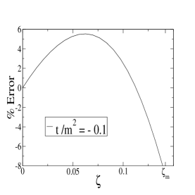
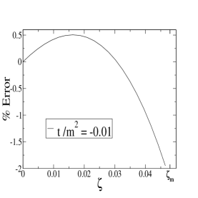
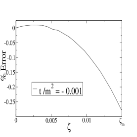
Figure 9: Verification of the sum rule in the non-relativistic limit. The percent error in the determination of the form factor (from the valence region SPD) plotted as a function of $\zeta$ for small values of $-t/m^{2}$.

Despite being suppressed by powers of $\alpha$ relative to the valence region, we can still look at the SPD’s structure in the non-valence region (Eq. 47). The coefficient functions $C_{b}(\zeta,t)$ and $C_{c}(\zeta,t)$ can both be calculated for small $\zeta$ and $-t/m^{2}$: we find $C_{b}\sim+N\zeta^{4}/8$ and $C_{c}\sim-N\zeta^{2}\times 10^{3}$, where $N=0.00545$ is the normalization constant appearing in Eq. 57 (determined with $\alpha=0.08$). Thus apart from variation with $\zeta$ we can ascertain the non-valence SPD’s behavior from $\int I\operatorname{D_{\text{W}}}$. In Figure 10 we plot $f(X,\zeta)\equiv-\frac{1}{\alpha}\int\frac{d\operatorname{\mathbf{k}^{\perp}}}{\sigma(1-\sigma)}I(\sigma,\operatorname{\mathbf{k}^{\perp}}|t)\operatorname{D_{\text{W}}}(\sigma,\operatorname{\mathbf{k}^{\perp}}|t)$ as a function of $X$ for fixed $\zeta$. The choice of sign preserves the overall sign of $\mathcal{F}$. The figure shows the SPD is symmetrical about $X=\zeta/2$ arising from the symmetry of $I$ and $\operatorname{D_{\text{W}}}$ about $\sigma=1/2$ (which in turn is due to the fact that our quarks are equally massive). Of course, as a function of $\sigma\in(0,1)$ the profile in the figure is universal. Given the nature of $C_{b}$ and $C_{c}$, since the scaled function $f(X,\zeta)$ is of order unity, the non-valence SPD is $\sim 10^{6}$ times smaller than the valence SPD for small $\zeta$ and $-t/m^{2}$ (here we use $\zeta=0.1$ for the comparison). The additional suppression (beyond powers of the weak coupling) is due to accessing the highly concentrated wave function near the end points.

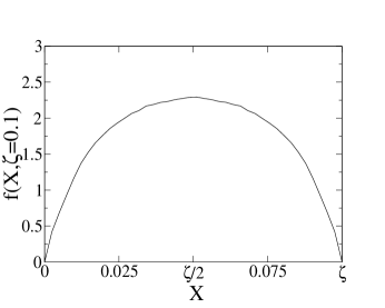
Figure 10: Structure of the non-valence SPD in the non-relativistic limit $-t/m^{2}\ll 1$. Here we plot $f(X,\zeta)$ (which is proportional to $\int I\operatorname{D_{\text{W}}}$ appearing in Eq. (47)) for the fixed value $\zeta=0.1$.

Using the non-relativistic limit to verify the sum rule is surely a good start, however, it does away with many of the complications inherent to the light-front approach. Were we to use the full solution to the Wick-Cutkosky model, not only would we have to worry about a consistent approximation scheme for the Green’s function, but also the lack of covariance (here rotational invariance). The above expression Eq. (42) is exact and consequently covariant (although not manifestly so), but using any realistic procedure to solve for the wave function, we must truncate the interaction kernel. Doing so we loose covariance, which is approximately restored only when our approximations to the kernel are improved [36]. This loss of rotational invariance would not only lead to improperly non-degenerate spectra but also would tamper with the sum rule. Without manifest Lorentz covariance, Eq. (22) will only be approximately satisfied and a true challenge to verify exactly. This is a difficulty which plagues any Hamiltonian theory.

9 Conclusion and outlook

Above we have seen how to express the pion’s skewed parton distribution in terms of two body, light-front wave functions. By using a light-front reduced Bethe-Salpeter approach, we can express the SPD in terms of two body wave functions by crossing the interaction (and making the assumption that the effective $qq$ potential is independent of energy). We did so first using only bare-coupling at the photon vertex. The functional form derived Eqs. (24,27) is time reversal invariant (as we explained how to demonstrate through $\xi$ symmetry) and is continuous at the crossover. In this non-perturbative scheme, however, the bare-coupling photon vertex is not justified and thus we derived the photon vertex function Eq. 38 in order to include the necessary $qq$ interactions and hence the effect of higher Fock states. The interacting theory SPD (42) can then be written in terms of two body wave functions and the Green’s function. The form derived maintains the necessary symmetry properties and is continuous. Potential schemes for approximating the Green’s function were then investigated. We found the Born approximation to the photon vertex does not result in the bare-coupling SPD since the diagram corresponding to $\mathcal{F}_{c}$ Eq. (41) is neglected. The non-relativistic approximation (47) and the closure approximation (7.2) to the non-valence region were then derived.

Using the non-relativistic approximation, we were able to verify the sum rule for the Wick-Cutkosky model in the weak binding limit (see Figure 9). Utilizing the crossed-pair potential and the non-relativistic approximation scheme, we explored SPD’s in the non-valence region (see Figure 10). This approach indeed provides an alternative to the explicit $N$-body Fock space expansion, and hence a different interpretation of the contributions to the valence and non-valence regions. We believe this paradigm is the most useful intuitively, though currently suffers from calculational intractability. For instance: the mass squared dependence of the interaction has been neglected here (as is often the case elsewhere, e.g. constituent quark models) and remains a crucial issue to be dealt with, not only in the context of these distributions but for form factors and quark distribution functions as well. Additionally calculation of the full four-point Green’s function presents another technical challenge. The closure approximation may however provide a way to reasonably approximate the Green’s function, since continuity and the sum rule can be used as constraints to check how well the full Hamiltonian can be described by the two-body sector. Lastly, we find that use of the crossed-pair potential in tandem with the Green’s function for the interacting theory allows one to obtain non-wave function vertices present in SPD’s and time-like form factors.

Acknowledgment

We thank J. R. Cooke for insight about one-boson exchange potentials and the Wick-Cutkosky model. This work was funded by the U. S. Department of Energy, grant: DE-FG$03-97$ER$41014$.

Appendix A: $\xi$ symmetry

At best, demonstrating the $\xi$ symmetry of our SPD’s is subtle. To keep matters simple, we consider only the bare-coupling SPD’s of section 4 and neglect quark self interactions, since their inclusion is straightforward and tangential to time-reversal invariance. While Eq. 25 is clearly even in $\xi$, the sign of $\Delta^{+}$ has been reversed and thus the location of the poles changed. Thus the whole derivation isn’t necessarily valid for $\xi\to-\xi$. Furthermore, directly switching $\xi\to-\xi$ in equation 29 yields zero. The time-reversal properties of our results are a crucial guide to consistency. Separately calculating the time-reversed diagrams of Figures 3 and 4, we easily arrive at the complex conjugates of Eqs. 25, 29. In order to show the relation between $\xi$-symmetry and time-reversal, we recalculate the covariant triangle diagram with $\Delta\to-\Delta$.

Looking at Figure 3 with $\Delta$ replaced with $-\Delta$, we have the following expression for the covariant diagram

$$-i\int\frac{d^{4}k}{(2\pi)^{4}}\frac{(2\operatorname{k^{+}}-\Delta^{+})\Gamma(k,P)\Gamma^{*}(k-\Delta,P-\Delta)}{(k^{2}-m^{2}+\operatorname{i\epsilon})((k-\Delta)^{2}-m^{2}+\operatorname{i\epsilon})((P-k)^{2}-m^{2}+\operatorname{i\epsilon})}.$$ (58)

Having reversed the sign of $\Delta^{+}$ in the diagram, we can again choose $\Delta^{+}\equiv-2\xi\operatorname{\bar{P}^{+}}\leq 0$, where $\xi>0$ and thus we have effectively taken $\xi$ here to be $-\xi$ of our previous calculation. Due to the kinematics, however, $\operatorname{P^{+}}=(1-\xi)\operatorname{\bar{P}^{+}}$. Thus defining $\Delta^{+}=-\Omega\operatorname{P^{+}}$ yields $\Omega=\frac{2\xi}{1-\xi}$. This should be compared to the skewness $\zeta=\frac{2\xi}{1+\xi}$. We still choose to work in the symmetrical frame, however, this constraint now reads $\operatorname{\mathbf{P}^{\perp}}=\Delta^{\perp}/2$ which is natural given the relative sign difference.

The poles of the $k^{-}$ integrand are situated at

$$\begin{cases}k_{a}^{-}=\Delta^{-}+\frac{m^{2}+(\operatorname{\mathbf{k}^{\perp}}-\Delta^{\perp})^{2}}{2(\operatorname{k^{+}}-\Delta^{+})}-\frac{\operatorname{i\epsilon}}{2(\operatorname{k^{+}}-\Delta^{+})}\\ k_{b}^{-}=\frac{m^{2}+\operatorname{\mathbf{k}^{\perp}}{}^{2}}{2\operatorname{k^{+}}}-\frac{\operatorname{i\epsilon}}{2\operatorname{k^{+}}}\\ k_{c}^{-}=P^{-}-\frac{m^{2}+(\operatorname{\mathbf{P}^{\perp}}-\operatorname{\mathbf{k}^{\perp}})^{2}}{2(\operatorname{P^{+}}-\operatorname{k^{+}})}+\frac{\operatorname{i\epsilon}}{2(\operatorname{P^{+}}-\operatorname{k^{+}})}.\end{cases}$$

When $\operatorname{k^{+}}<\Delta^{+}$, all poles lie in the upper-half complex plane and when $\operatorname{k^{+}}>\operatorname{P^{+}}$, all poles lie in the lower-half plane. Thus, by Cauchy, these contributions to the integral vanish. Now we consider the non-zero contributions.

Firstly we unravel the familiar case: $0<\operatorname{k^{+}}<\Delta^{+}$ which gives a contribution $2\pi i\operatorname{Res}(k_{c}^{-})$. At this point, however, the region appears far from familiar. The ratio $\operatorname{k^{+}}/P^{+}$ is restricted to $(0,1)$. To relate with our previous notation, we must define $\operatorname{k^{+}}/\operatorname{P^{+}}\equiv Y=\frac{x-\xi}{1-\xi}$ which restricts $x\in(\xi,1)$.

Using the definition established in equation 20, we merely strip away the $\operatorname{k^{+}}$ integral as well as the coupling to uncover

$$\operatorname{\mathcal{F}(X,\zeta,t)}=\int\frac{d\operatorname{\mathbf{k}^{\perp}}}{2(2\pi)^{3}}\frac{1}{Y(Y+\Omega)(1-Y)}\frac{\Gamma(Y,\operatorname{\mathbf{k}^{\perp}}-Y\Delta^{\perp}/2)}{2\operatorname{P^{+}}P^{-}-\frac{m^{2}+\operatorname{\mathbf{k}^{\perp}}{}^{2}}{Y}-\frac{m^{2}+(\operatorname{\mathbf{k}^{\perp}}-\Delta^{\perp}/2)^{2}}{1-Y}}\\ \times\frac{\Gamma^{*}\Big{(}\frac{Y+\Omega}{1+\Omega},\operatorname{\mathbf{k}^{\perp}}+\big{(}\frac{1}{2}\frac{Y+\Omega}{1+\Omega}-1\big{)}\Delta^{\perp}\Big{)}}{2\operatorname{P^{+}}(P^{-}-\Delta^{-})-\frac{m^{2}+(\operatorname{\mathbf{k}^{\perp}}-\Delta^{\perp})^{2}}{Y+\Omega}-\frac{m^{2}+(\operatorname{\mathbf{k}^{\perp}}-\Delta^{\perp}/2)^{2}}{1-Y}}.$$ (59)

Simple algebra gives the relation $\frac{Y+\Omega}{1+\Omega}=\frac{x+\xi}{1+\xi}=X$. As before we can use $\Delta^{-}=\frac{t+\Delta^{\perp}{}^{2}}{2\Delta^{+}}$ to write $2\operatorname{P^{+}}\Delta^{-}=-(t+\Delta^{\perp}{}^{2})/\Omega$. (Back in section 4, this relation was strikingly similar $2\operatorname{P^{+}}\Delta^{-}=-(t+\Delta^{\perp}{}^{2})/\zeta$.) We then exploit $\Delta\cdot\bar{P}=0$ to find

$$-t=\frac{(1+\Omega/2)^{2}\Delta^{\perp}{}^{2}+\Omega^{2}M^{2}}{1+\Omega},$$ (60)

which relates to the expression earlier by $\Omega\to-\zeta$. Using the above, we can write $2\operatorname{P^{+}}\Delta^{-}=\Omega(M^{2}+\frac{1}{4}\Delta^{\perp}{}^{2})/(1+\Omega)$. (Back in section 4, we used the relation $2\operatorname{P^{+}}\Delta^{-}=\zeta(M^{2}+\frac{1}{4}\Delta^{\perp}{}^{2})/(1-\zeta)$.)

Identification of the initial meson’s wave function in Eq. 59 is simple

$$\frac{\Gamma(Y,\operatorname{\mathbf{k}^{\perp}}-Y\Delta^{\perp}/2)}{2\operatorname{P^{+}}P^{-}-\frac{m^{2}+\operatorname{\mathbf{k}^{\perp}}{}^{2}}{Y}-\frac{m^{2}+(\operatorname{\mathbf{k}^{\perp}}-\Delta^{\perp}/2)^{2}}{1-Y}}=\psi(Y,\operatorname{\mathbf{k}^{\perp}}-Y\Delta^{\perp}/2).$$ (61)

The final meson’s wave function requires us to manipulate the energy denominator

$$2\operatorname{P^{+}}(P^{-}-\Delta^{-})-\frac{m^{2}+(\operatorname{\mathbf{k}^{\perp}}-\Delta^{\perp})^{2}}{Y+\Omega}-\frac{m^{2}+(\operatorname{\mathbf{k}^{\perp}}-\Delta^{\perp}/2)^{2}}{1-Y}=\frac{1}{1+\Omega}\Big{(}M^{2}-\frac{m^{2}+(\operatorname{\mathbf{k}^{\perp}}+(X/2-1)\Delta^{\perp})^{2}}{X(1-X)}\Big{)}.$$ (62)

Upon shifting the $\operatorname{\mathbf{k}^{\perp}}$ integral, we arrive at

$$\operatorname{\mathcal{F}(X,\zeta,t)}=\int\frac{d\operatorname{\mathbf{k}^{\perp}}}{2(2\pi)^{3}}\frac{1+\Omega}{Y(Y+\Omega)(1-Y)}\psi(Y,\operatorname{\mathbf{k}^{\perp}}+(1-\bar{x})\Delta^{\perp})\psi^{*}(X,\operatorname{\mathbf{k}^{\perp}}).$$ (63)

The pre-factors along with the conversion factor $1-\xi$

$$(1-\xi)\frac{1+\Omega}{Y(Y+\Omega)(1-Y)}=\frac{1-\xi^{2}}{(x^{2}-\xi^{2})(1-x)}$$ (64)

identically line up to our expression 25 and thus we see why the naïve replacement $\xi\to-\xi$ was justified.

Lastly we consider the region $\Delta^{+}<\operatorname{k^{+}}<0$. Given our identification of $Y$ as $\operatorname{k^{+}}/\operatorname{P^{+}}$, we see $x$ is restricted to $(-\xi,\xi)$. To evaluate the integral Eq. 58 in this régime, we calculate $-2\pi i\operatorname{Res}(k_{a}^{-})$. From this expression, we toss away the $\operatorname{k^{+}}$ integral to uncover

$$\operatorname{\mathcal{F}(X,\zeta,t)}=\int\frac{d\operatorname{\mathbf{k}^{\perp}}}{2(2\pi)^{3}}\frac{1}{Y(Y+\Omega)(1-Y)}\frac{\Gamma(Y,\operatorname{\mathbf{k}^{\perp}}-Y\Delta^{\perp}/2)}{2\operatorname{P^{+}}\Delta^{-}-\frac{m^{2}+\operatorname{\mathbf{k}^{\perp}}{}^{2}}{Y}+\frac{m^{2}+(\operatorname{\mathbf{k}^{\perp}}-\Delta^{\perp})^{2}}{Y+\Omega}}\\ \times\frac{\Gamma^{*}(X,\operatorname{\mathbf{k}^{\perp}}+(X/2-1)\Delta^{\perp})}{2\operatorname{P^{+}}(P^{-}-\Delta^{-})-\frac{m^{2}+(\operatorname{\mathbf{k}^{\perp}}-\Delta^{\perp})^{2}}{Y+\Omega}-\frac{m^{2}+(\operatorname{\mathbf{k}^{\perp}}-\Delta^{\perp}/2)^{2}}{1-Y}}.$$ (65)

Comparing with our above equation (59) the final state meson vertex and energy denominator are unchanged and can thus be replaced by $(1+\Omega)\psi^{*}(X,\operatorname{\mathbf{k}^{\perp}}+(X/2-1)\Delta^{\perp})$.

A little algebra needs to be employed to see

$$2\operatorname{P^{+}}\Delta^{-}-\frac{m^{2}+\operatorname{\mathbf{k}^{\perp}}{}^{2}}{Y}+\frac{m^{2}+(\operatorname{\mathbf{k}^{\perp}}-\Delta^{\perp})^{2}}{Y+\Omega} =-\frac{1}{\Omega}\Big{(}t+\frac{m^{2}+(\operatorname{\mathbf{k}^{\perp}}+\frac{Y}{\Omega}\Delta^{\perp})^{2}}{\frac{Y}{\Omega}(\frac{Y}{\Omega}-1)}\Big{)}$$

$$=-\frac{1}{\Omega}\Big{(}t-\frac{m^{2}+(\operatorname{\mathbf{k}^{\perp}}+(\sigma-1)\Delta^{\perp})^{2}}{\sigma(1-\sigma)}\Big{)},$$ (66)

where we used the relation $Y/\Omega=X/\zeta-1=\sigma-1$.

Now in Eq. 65, the initial meson’s vertex can be related to a wave function only by using the interaction’s crossing symmetry (since $Y<0$). Writing the remaining vertex in terms of the interaction, as well shifting the $\operatorname{\mathbf{k}^{\perp}}$ integral by $\Delta^{\perp}$ we see

$$\operatorname{\mathcal{F}(X,\zeta,t)}=\frac{-\Omega(1+\Omega)}{Y(Y+\Omega)(1-Y)}\int\frac{d\operatorname{\mathbf{k}^{\perp}}dZd\operatorname{\mathbf{\kappa}^{\perp}}}{[2(2\pi)^{3}]^{2}Z(1-Z)}\psi(Z,\operatorname{\mathbf{\kappa}^{\perp}})\\ \times V\Big{(}Z,\operatorname{\mathbf{\kappa}^{\perp}};Y,\operatorname{\mathbf{k}^{\perp}}+(1-Y/2)\Delta^{\perp}\Big{)}\operatorname{D_{\text{W}}}(\sigma,\operatorname{\mathbf{k}^{\perp}}+\sigma\Delta^{\perp}|t)\psi^{*}(X,\operatorname{\mathbf{k}^{\perp}}+X\Delta^{\perp}/2).$$ (67)

For suspense, we have saved the pre-factors (and conversion factor) till the very end

$$-(1-\xi)\frac{\Omega(1+\Omega)}{Y(Y+\Omega)(1-Y)}=-\frac{2\xi(1+\xi)}{(x^{2}-\xi^{2})(1-x)}.$$ (68)

The $\xi$ symmetry of equation 29 has been demonstrated and thus the covariant approach naturally incorporates the subtlety of switching the $q\bar{q}$ pair annihilation from the initial to final state when $\xi\to-\xi$. This algebra can easily be extended once interactions have been added at the photon vertex.

Appendix B: SPD’s, form factors and quark distributions

Above we have made reference to verifying the sum rule Eq. (22) without specifying what structure the form factor has. Here we connect our expressions for SPD’s to the celebrated Drell-Yan-West formula for the form factor [37] and then analyze what neglecting the energy dependence of the $qq$ interaction has done to SPD’s, form factors and quark distributions.

Since Lorentz covariance constrains the $X$ integral of the SPD’s to be independent of $\zeta$, we may find the electromagnetic form factor by integrating the SPD’s in the limit of zero skewness ($\zeta\to 0$). This corresponds to using the highly simplifying Drell-Yan-West frame in which the plus component of the photon’s momentum vanishes (here $\Delta^{+}=0$). This limit is now complicated by possible singularities arising from the non-valence region ($X<\zeta$), like those encountered in [26]. Ignoring this complication for the moment, we see the contribution from the valence region ($X>\zeta$) gives

$$\lim_{\zeta\to 0}\int_{\zeta}^{1}X\mathcal{F}_{a}(X,\zeta,t)dX=\int\frac{dXd\operatorname{\mathbf{k}^{\perp}}\theta[X(1-X)]}{2(2\pi)^{3}X(1-X)}\psi(X,\operatorname{\mathbf{k}^{\perp}})\psi^{*}\big{(}X,\operatorname{\mathbf{k}^{\perp}}+(1-X)\Delta^{\perp}\big{)}$$ (69)

the Drell-Yan-West formula.

It is interesting to first consider the non-valence contribution to the form factor coming from the bare-coupling SPD (Eq. 27). As this region extends from $X=0$ to $\zeta$, to avoid singular momentum fractions, we change variables from $X$ to $\sigma=X/\zeta$ and then take the limit in which $\zeta$ vanishes. The contribution to the form factor reads

$$\lim_{\zeta\to 0}\int_{0}^{\zeta}X\operatorname{\mathcal{F}(X,\zeta,t)}dX\sim\zeta\;\int\frac{d\sigma\;d\operatorname{\mathbf{k}^{\perp}}dZd\operatorname{\mathbf{\kappa}^{\perp}}}{[2(2\pi)^{3}]^{2}(1-\sigma)Z(1-Z)}\psi(\zeta\;\sigma,\operatorname{\mathbf{k}^{\perp}})\\ \times\operatorname{\Delta_{\text{W}}}\Big{(}\sigma,\operatorname{\mathbf{k}^{\perp}}+\sigma\Delta^{\perp}\Big{|}t\Big{)}V\Big{(}Z,\operatorname{\mathbf{\kappa}^{\perp}};\zeta(\sigma-1),\operatorname{\mathbf{k}^{\perp}}+\Delta^{\perp}\Big{)}\psi^{*}(Z,\operatorname{\mathbf{\kappa}^{\perp}})$$ (70)

which vanishes as $\zeta\;\psi(\zeta\;\sigma,\ldots)$ as $\zeta\to 0$. Thus for the Born approximation to the photon vertex, the Drell-Yan-West formula indeed gives the form factor.

We can, of course, employ the same change of variables technique to consider the contributions to the electromagnetic form factor from the true SPD’s of section 6. The contribution from $\mathcal{F}_{b}(X,\zeta,t)$ Eq. (39) proceeds very similarly to the analysis for the bare-coupling SPD above. Additionally we must change variables from $W\in(0,\zeta)$ to $\omega=W/\zeta$ but in the end $\int X\;\mathcal{F}_{b}\;dX\sim\zeta\;\psi(\zeta\;\omega,\ldots)$ as $\zeta\to 0$.

Lastly we consider the possible contribution from $\mathcal{F}_{c}(X,\zeta,t)$ Eq. (41). The change of variables from $X$ to $\zeta$ runs as above. On the other hand, $W\in(\zeta,1)$ giving us no reason for an addition change to $\omega$. Taking $\zeta$ to zero results in $\int X\;\mathcal{F}_{c}\;dX\sim\zeta\;V\Big{(}\frac{W}{\zeta},\frac{W}{\zeta}\Delta^{\perp};\ldots\Big{)}$ where $V$ is the crossed potential defined for a momentum fraction greater than one. Using the crossed potential for the Wick-Cutkosky model, this contribution to the form factor vanishes as $\zeta^{2}$.

We have shown that both contributions $b$ and $c$ vanish in the limit of zero skewness. Within the impulse approximation, the Drell-Yan-West formula for the form factor is exact for our model. Thus we have seen, whether or not we include interactions at the photon vertex our model has the same form factor. The procedure here can be straightforwardly applied to the SPD’s in the approximation schemes of section 7. For precisely the same reasons above, both schemes preserve the Drell-Yan-West formula in the forward limit.

Having demonstrated there are no singularities associated with the limit $\zeta\to 0$, we can also extract our model’s quark distribution function $q(x)\equiv F(x,0,0)$. This is then simply the forward limit of Eq. 24, namely

$$q(x)=\int\frac{d\operatorname{\mathbf{k}^{\perp}}}{2(2\pi)^{3}x(1-x)}|\psi(x,\operatorname{\mathbf{k}^{\perp}})|^{2}$$ (71)

the square of the meson’s wave function. In light of our above analysis, we know that the wave function vanishes quadratically at the end points and thus $q(x)$ vanishes there as well. This is physical at $x=1$ since one parton cannot posses all of the meson’s plus momentum. At $x=0$, however, the non-valence partons can rescue one parton from carrying all the plus momentum and so such configurations have non-zero probability, i.e. $q(0)\neq 0$. Indeed the fact that our model distributions vanish at $x=0$ is tied directly to neglecting the mass squared dependence of the effective interaction in the two-body subspace. The non-valence probability amplitude $\langle\psi_{\text{nv}}|\psi_{\text{nv}}\rangle$ is simply

$$\langle\psi_{\text{nv}}|\psi_{\text{nv}}\rangle=-\frac{\partial}{\partial M^{2}}\langle\psi_{2}|V|\psi_{2}\rangle,$$ (72)

where $\langle\psi_{2}|V|\psi_{2}\rangle$ is the projection of the interaction on the two-body subspace (simply denoted as $V$ above).

Accounting for the mass squared dependence of the effective interaction allows for non-valence contributions to the quark distribution functions. There are further consequences, however, given the unifying role of SPD’s. The Drell-Yan-West formula, for example, will have corrections (of particular importance to the form factor’s $x$-integrand at small $x$), and adding interactions at the photon vertex will then change the form factor. It has already been noticed [38] that model deuteron wave functions have better covariance properties than their form factors calculated from Drell-Yan-West expressions. Lastly the most general consequence is to affect the SPD’s, particularly at the crossover, e.g. $F(\zeta,\zeta,t)=0$ seen here (as well as in [11, 12]) stems directly from neglecting the mass squared dependence. The crossover point thus probes a convolution of non-valence states for which this approach may possibly be apt in describing, however, it would require a reworking of the photon vertex that does not make use of the potential model’s Green’s function. (As for the light-cone Fock space expansion, calculation of wave functions at small $x$ is rather complicated but contains rich information about the relation between different Fock components [39].)

Appendix C: GDA’s and the time-like form factor

Time-like form factors have been often avoided in the light-front approach due to the unavoidable presence of non-wave function vertices. This complication is mirrored in the scheme of [17]: the time-like pion form factor does not have a direct decomposition in terms of pion Fock component overlaps alone. Here we show how the above analysis can be applied to time-like form factors; that is, we obtain expressions in terms of two-body Bethe-Salpeter wave functions and the four-point Green’s functions. Furthermore, we make the connection with the generalized distribution amplitude for our model which encodes the non-perturbative physics of two pion production [24, 25]. We attempt below to preserve the notation set up in these references.

Figure 11: The triangle diagram for the time-like, pion form factor

The time-like pion form factor $F(s)$ is defined by (see Figure 11)

$$\langle\pi(p)\;\pi(\operatorname{p^{\prime}})\;|\;J^{\mu}(0)\;|\;0\;\rangle=(p-\operatorname{p^{\prime}})^{\mu}F(s),$$ (73)

where $s=(p+\operatorname{p^{\prime}})^{2}$ is the center of mass energy squared. Here the pion is merely our $qq$ pair. Now define $P^{\mu}=p^{\mu}+\operatorname{p^{\prime}}^{\mu}$ and $\zeta=\operatorname{p^{+}}/\operatorname{P^{+}}$. We can work out the kinematics of this reaction to find

$$P^{-} =\frac{s}{2\operatorname{P^{+}}}$$

$$p^{-} =\frac{(1-\zeta)s}{2\operatorname{P^{+}}}$$

$$\operatorname{\mathbf{p}^{\perp}}{}^{2} =s(1-\zeta)\zeta-M^{2},$$ (74)

where $M$ is the pion mass and we work in the frame in which $\mathbf{P}^{\perp}=0$. .

The GDA for our model has a definition in terms of a non-diagonal matrix element of bi-local field operators

$$\operatorname{\Phi(z,\zeta,s)}=\int\frac{dx^{-}e^{iz\operatorname{P^{+}}x^{-}}}{2\pi(2z-1)}\langle\;\pi(p)\;\pi(\operatorname{p^{\prime}})\;|\;q(x^{-})\overset{\leftrightarrow}{\partial}{}^{+}q(0)\;|0\;\rangle.$$ (75)

Such a definition of the GDA leads us immediately to the sum rule

$$\int\frac{2z-1}{2\zeta-1}\operatorname{\Phi(z,\zeta,s)}dz=F(s),$$ (76)

and hence a means to calculate $\Phi$ from the integrand of the time-like form factor.

Returning to Figure 11, we can write down the expression for the time-like form factor

$$-i\int\frac{d^{4}k}{(2\pi)^{4}}\Gamma^{+}(k,P)G_{o}(k)\Gamma(k,p)G_{o}(k-p)\Gamma(k-p,P-p)G_{o}(k-P)$$ (77)

and perform the light-front reduction by integrating out the minus dependence. Whenever troublesome momentum fractions appear, we use the equation of motion (2) to insert the crossed interaction. Lastly we merely extract the derivative coupling and $z$-integral from the photon vertex function to uncover the GDA. Using $w\equiv\operatorname{k^{+}}/\operatorname{P^{+}}$, the relevant contribution from the photon vertex appears as

$$\delta(q^{+}-z\operatorname{P^{+}})\frac{i\Gamma^{+}(k,P)}{(2z-1)\operatorname{P^{+}}}\operatorname{\Delta_{\text{W}}}(w,\operatorname{\mathbf{k}^{\perp}}|s)=\int\frac{d\operatorname{\mathbf{q}^{\perp}}}{2(2\pi)^{3}z(1-z)}G(z,\operatorname{\mathbf{q}^{\perp}};w,\operatorname{\mathbf{k}^{\perp}}|s),$$ (78)

with $z\in(0,1)$.

Carrying out this evaluation yields

$$\operatorname{\Phi(z,\zeta,s)}=\int\frac{d\operatorname{\mathbf{q}^{\perp}}dwd\operatorname{\mathbf{k}^{\perp}}dxd\operatorname{\mathbf{\kappa}^{\perp}}}{[2(2\pi)^{3}]^{3}w(w-\zeta)(1-w)x(1-x)z(1-z)}\psi(x,\operatorname{\mathbf{\kappa}^{\perp}})G(z,\operatorname{\mathbf{q}^{\perp}};w,\operatorname{\mathbf{k}^{\perp}}|s)\\ \times\Bigg{(}\phi_{a}(w,\operatorname{\mathbf{k}^{\perp}};x,\operatorname{\mathbf{\kappa}^{\perp}})\;\theta[w(\zeta-w)]+\phi_{b}(w,\operatorname{\mathbf{k}^{\perp}};x,\operatorname{\mathbf{\kappa}^{\perp}})\;\theta[(1-w)(w-\zeta)]\Bigg{)}$$ (79)

where we have abbreviated

$$\phi_{a}(w,\operatorname{\mathbf{k}^{\perp}};x,\operatorname{\mathbf{\kappa}^{\perp}}) =\zeta\;V\Big{(}x,\operatorname{\mathbf{\kappa}^{\perp}};y,\operatorname{\mathbf{k}^{\perp}}+(1-y)\operatorname{\mathbf{p}^{\perp}}\Big{)}\psi\Big{(}\frac{w}{\zeta},\operatorname{\mathbf{k}^{\perp}}-\frac{w}{\zeta}\operatorname{\mathbf{p}^{\perp}}\Big{)}$$

$$\phi_{b}(w,\operatorname{\mathbf{k}^{\perp}};x,\operatorname{\mathbf{\kappa}^{\perp}}) =(\zeta-1)\;V\Big{(}x,\operatorname{\mathbf{\kappa}^{\perp}};\frac{w}{\zeta},\operatorname{\mathbf{k}^{\perp}}-\frac{w}{\zeta}\operatorname{\mathbf{p}^{\perp}}\Big{)}\psi\Big{(}y,\operatorname{\mathbf{k}^{\perp}}+(1-y)\operatorname{\mathbf{p}^{\perp}}\Big{)},$$ (80)

with $y=\frac{w-\zeta}{1-\zeta}$. The two contributions ($a$ and $b$) to the GDA can be interpreted graphically, see Figure 12.

Δ

$=$ Θ $+$ Λ

Figure 12: Graphical representation of contributions to the GDA Eq. (79): $\Phi=\phi_{a}+\phi_{b}$. The shaded box again represents the crossed interaction and the internal double line represents the four-point Green’s function.

We can furthermore decompose the GDA in the approximation schemes set forth in section 7. In the non-relativistic scheme, we use the approximation to the Green’s function in Eq. 46 to derive

$$\operatorname{\Phi(z,\zeta,s)}^{\text{NR}}=\Bigg{(}\phi_{a}^{\text{NR}}(\zeta,s)\;\theta\big{[}\zeta-\frac{1}{2}\big{]}+\phi_{b}^{\text{NR}}(\zeta,s)\;\theta\big{[}\frac{1}{2}-\zeta\big{]}\Bigg{)}\int\frac{d\operatorname{\mathbf{q}^{\perp}}}{2(2\pi)^{3}z(1-z)}I(z,\operatorname{\mathbf{q}^{\perp}}|s)\operatorname{D_{\text{W}}}(z,\operatorname{\mathbf{q}^{\perp}}|s),$$ (81)

where

$$\phi_{a}^{\text{NR}}(\zeta,s) =\frac{\zeta}{\frac{1}{2}-\zeta}\psi(\mathbf{r}=0)V\Big{(}\frac{1}{2},\mathbf{0}^{\perp};\frac{\frac{1}{2}-\zeta}{1-\zeta},-\frac{\operatorname{\mathbf{p}^{\perp}}/2}{1-\zeta}\Big{)}\psi\Big{(}\frac{1}{2\zeta},-\frac{\operatorname{\mathbf{p}^{\perp}}}{2\zeta}\Big{)}$$

$$\phi_{b}^{\text{NR}}(\zeta,s) =-\frac{1-\zeta}{\frac{1}{2}-\zeta}\psi(\mathbf{r}=0)V\Big{(}\frac{1}{2},\mathbf{0}^{\perp};\frac{1}{2\zeta},-\frac{\operatorname{\mathbf{p}^{\perp}}}{2\zeta}\Big{)}\psi\Big{(}\frac{\frac{1}{2}-\zeta}{1-\zeta},-\frac{\operatorname{\mathbf{p}^{\perp}}/2}{1-\zeta}\Big{)},$$ (82)

where $\psi(\mathbf{r}=0)$ is defined in Eq. 49. In this form, we see the non-relativistic approximation maintains continuity at $\zeta=1/2$. Apart from $\zeta$ dependent coefficients, the structure of the non-relativistic GDA is identical to that of the non-relativistic SPD in the non-valence region (with $\sigma$ replaced with $z$), see Eq. (47).

Lastly appealing to the closure approximation for the Green’s function, we arrive at the approximate GDA

$$\operatorname{\Phi(z,\zeta,s)}^{\text{CL}}=\int\frac{d\operatorname{\mathbf{q}^{\perp}}dxd\operatorname{\mathbf{\kappa}^{\perp}}}{[2(2\pi)^{3}]^{3}z(1-z)(z-\zeta)x(1-x)}\psi(x,\operatorname{\mathbf{\kappa}^{\perp}})\\ \times\Bigg{(}\frac{\phi_{a}(z,\operatorname{\mathbf{q}^{\perp}};x,\operatorname{\mathbf{\kappa}^{\perp}})}{s-\operatorname{\langle\mu^{2}\rangle}_{a}}\theta[z(\zeta-z)]+\frac{\phi_{b}(z,\operatorname{\mathbf{q}^{\perp}};x,\operatorname{\mathbf{\kappa}^{\perp}})}{s-\operatorname{\langle\mu^{2}\rangle}_{b}}\theta[(1-z)(z-\zeta)]\Bigg{)}.$$ (83)

Notice given the form of the functions Appendix C: GDA’s and the time-like form factor, the closure approximation to the GDA is continuous at $z=\zeta$. This is a curious fact (in contrast to SPD’s) since the factorization theorem for GDA’s does not depend on continuity at $z=\zeta$ [25]. Additionally at large $s$, we can apply the Born approximation to the Green’s function. The resulting GDA’s are identical to bare-coupling GDA’s, which is a further contrast to SPD’s.

References

- [1] D. Müller, D. Robaschik, B. Geyer, F. M. Dittes and J. Hořejši, Fortsch. Phys. 42, 101 (1994) [hep-ph/9812448].
- [2] X. Ji, Phys. Rev. Lett. 78, 610 (1997); Phys. Rev. D 55, 7114 (1997)
- [3] A. V. Radyushkin, Phys. Rev. D 56, 5524 (1997)
- [4] X. Ji and J. Osborne, Phys. Rev. D 58, 094018 (1998)
- [5] J. C. Collins and A. Freund, Phys. Rev. D 59, 074009 (1999)
- [6] A. V. Radyushkin, Phys. Lett. B 385, 333 (1996)
- [7] J. C. Collins, L. Frankfurt and M. Strikman, Phys. Rev. D 56, 2982 (1997)
- [8] L. Frankfurt, G. A. Miller and M. Strikman, hep-ph/0010297.
- [9] P. R. Saull [ZEUS Collaboration], hep-ex/0003030. L. Favart [H1 Collaboration], hep-ex/0101046. C. Adloff et al. [H1 Collaboration], Phys. Lett. B 517, 47 (2001) A. Airapetian et al. [HERMES Collaboration], Phys. Rev. Lett. 87, 182001 (2001) S. Stepanyan et al. [CLAS Collaboration], Phys. Rev. Lett. 87, 182002 (2001)
- [10] X. Ji, W. Melnitchouk and X. Song, Phys. Rev. D 56, 5511 (1997)
- [11] M. Diehl, T. Feldmann, R. Jakob and P. Kroll, Eur. Phys. J. C 8, 409 (1999)
- [12] M. Burkardt, Phys. Rev. D 62, 094003 (2000)
- [13] S. J. Brodsky, M. Diehl and D. S. Hwang, Nucl. Phys. B 596, 99 (2001)
- [14] V. Y. Petrov, P. V. Pobylitsa, M. V. Polyakov, I. Bornig, K. Goeke and C. Weiss, Phys. Rev. D 57, 4325 (1998)
- [15] M. Burkardt, Phys. Rev. D 62, 071503 (2000); M. Burkardt, hep-ph/0105324.
- [16] B. C. Tiburzi and G. A. Miller, Phys. Rev. C 64, 065204 (2001)
- [17] M. Diehl, T. Feldmann, R. Jakob and P. Kroll, Nucl. Phys. B 596, 33 (2001)
- [18] M. B. Einhorn, Phys. Rev. D 14, 3451 (1976).
- [19] H. M. Choi, C. R. Ji and L. S. Kisslinger, Phys. Rev. D 64, 093006 (2001)
- [20] S. J. Brodsky, C. Ji and M. Sawicki, Phys. Rev. D 32, 1530 (1985); J. H. Sales, T. Frederico, B. V. Carlson and P. U. Sauer, Phys. Rev. C 61, 044003 (2000)
- [21] P. A. Dirac, Rev. Mod. Phys. 21, 392 (1949); H. Leutwyler and J. Stern, Annals Phys. 112, 94 (1978).
- [22] C. D. Roberts and A. G. Williams, Prog. Part. Nucl. Phys. 33, 477 (1994)
- [23] S. Weinberg, Phys. Rev. 150, 1313 (1966).
- [24] M. Diehl, T. Gousset, B. Pire and O. Teryaev, Phys. Rev. Lett. 81, 1782 (1998); M. Diehl, T. Gousset and B. Pire, Phys. Rev. D 62, 073014 (2000)
- [25] M. V. Polyakov and C. Weiss, Phys. Rev. D 59, 091502 (1999); M. V. Polyakov, Nucl. Phys. B 555, 231 (1999)
- [26] Choosing the frame eliminates pair creation by a virtual photons. In general, this diagram is needed in order to maintain covariance and does not always vanish in the limit (especially relevant when one looks at bad components of the current operators, see B. L. G. Bakker and C.-R. Ji, Phys. Rev. D62, 074014 (2000) ). We will only be looking at good components of the current operators in the deeply virtual limit. Furthermore since our meson and quarks have low (zero) spin (see the consideration of two fermion, spin- composite systems in J. P. B. C. de Melo, T. Frederico, H. W. L. Naus, P. U. Sauer, Nucl. Phys. A660, 219 (1999) ), we do not expect any loss of covariance.
- [27] M. Sawicki, Phys. Rev. D 44, 433 (1991); Phys. Rev. D 46, 474 (1992).
- [28] Choosing now the symmetrical frame, the transverse momentum in section 4 is related to that in section 3 by a boost: .
- [29] In our previous work, we did not remove the derivative coupling at the photon vertex from the SPD. Thus we differ by a factor of in the numerator.
- [30] M. Diehl, T. Gousset, B. Pire and J. P. Ralston, Phys. Lett. B 411, 193 (1997)
- [31] C. G. Callan, N. Coote and D. J. Gross, Phys. Rev. D 13, 1649 (1976).
- [32] Alternatively, one could appeal to Eq. 5 to deal with the problematic momentum fractions. In this scheme, we insert the T-matrix instead of the Green’s function in the photon vertex function. The problematic momentum fraction gives rise to a crossed potential as well as a crossed T-matrix. To unravel the SPD’s in terms of two-body wave functions one utilizes the two potential theorem, and the final results are, of course, the same.
- [33] B. C. Tiburzi and G. A. Miller, Phys. Rev. C 63, 044014 (2001)
- [34] V. A. Karmanov, Nucl. Phys. B 166, 378 (1980); J. Carbonell, B. Desplanques, V. A. Karmanov and J. F. Mathiot, Phys. Rept. 300, 215 (1998)
- [35] J. R. Cooke and G. A. Miller, Phys. Rev. C 62, 054008 (2000)
- [36] J. R. Cooke, G. A. Miller and D. R. Phillips, Phys. Rev. C 61, 064005 (2000)
- [37] S. D. Drell and T. Yan, Phys. Rev. Lett. 24, 181 (1970); G. B. West, Phys. Rev. Lett. 24, 1206 (1970).
- [38] J. R. Cooke, University of Washington, Ph.D. Thesis, 2001 (to be published).
- [39] F. Antonuccio, S. J. Brodsky and S. Dalley, Phys. Lett. B 412, 104 (1997)