hep-ph/0109172 CERN–TH/2001–220 IFUP–TH/2001–22

Which solar neutrino experiment

after KamLAND and Borexino?

Alessandro Strumia^†

Theoretical Physics Division, CERN, CH-1211 Geneva 23, Switzerland

Francesco Vissani

INFN, Laboratori Nazionali del Gran Sasso, Theory Group, I-67010 Assergi (AQ), Italy

Abstract

We estimate how well we will know the parameters of solar neutrino oscillations after KamLAND and Borexino. The expected error on $\Delta m^{2}$ is few per-mille in the VO and QVO regions, few per-cent in the LMA region, and around $10\%$ in the LOW region. The expected error on $\sin^{2}2\theta$ is around $5\%$. KamLAND and Borexino will tell unambiguously which specific new measurement, dedicated to $pp$ solar neutrinos, is able to contribute to the determination of $\theta$ and perhaps of $\Delta m^{2}$. The present data suggest as more likely outcomes: no measurement, or the total $pp$ rate, or its day/night variation.

1 Introduction

The solar neutrino anomaly revealed in Homestake [1], Kamiokande [2], Gallex [3] and SAGE [4] has motivated the upgrades SuperKamiokande (SK) [5], GNO [6], and a new generation of experiments: SNO [7], KamLAND [8] and Borexino [9]. In the longer term, there are plans to attempt the real-time detection of $pp$ neutrinos, thus covering the whole solar neutrino spectrum [10]. Depending on the choice of experimental technique, it is hoped that future sub-MeV experiments will be able to measure some of the following properties of the solar neutrino flux at sub-MeV energies

• total rate;

• day/night variations;

• “seasonal” variations;

• energy spectrum;

• total rate in neutral and charge-current (NC and CC) reactions.

Today there are few disjoint best-fit solutions (usually named LMA, LOW, VO, …) and these measurements could identify the true one. In fact, the survival probabilities $P_{ee}(E_{\nu})$ for the present best-fit oscillations are not much different at $E_{\nu}\sim 10\,{\rm MeV}$ where we have more experimental data, but are significantly different at lower $E_{\nu}$.

However, these sub-MeV experiments will presumably start after SNO, KamLAND and Borexino have already identified the true solar-neutrino solution and determined the solar-neutrino oscillation parameters. In this case, one should change the perspective and evaluate the potential of new experiments to improve on the measurement of solar oscillation parameters — to be contrasted with “to prove the occurrence of oscillations”. From this point of view, we answer the question in the title by determining how well near-future experiments are expected to contribute to these measurements. This fixes the minimal necessary accuracy of new sub-MeV experiments.

The conclusions (see table 1 or fig. 1) crucially depend on the true value of the oscillation parameters $\Delta m^{2}$ and $\theta$. A sub-MeV detector able to do different measurements but only with modest accuracy is never relevant to the measurement of oscillations parameters. Conversely, certain specific sub-MeV measurement could be relevant, if done precisely enough. Near-future experiments are able to cover fairly well all the possible cases (often measuring $\Delta m^{2}$ with great precision), and will indicate unambiguously which is the remaining relevant sub-MeV measurement.

$$\begin{array}[]{|clcc|c|cccc|c|}\hline\cr\vrule\lx@intercol\hfil\hbox{Benchmark points}\hfil\lx@intercol\vrule\lx@intercol&\hbox{Present}&\vrule\lx@intercol\hfil\hbox{Estimated near-future uncertainty}\hfil\lx@intercol\vrule\lx@intercol&\hbox{Useful sub-MeV}\\ &\hbox{region}&\Delta m^{2}/\,{\rm eV}^{2}&\tan^{2}\theta&\chi^{2}-\chi^{2}_{\rm best}&\hbox{main experiment}&\delta\Delta m^{2}&\delta\tan^{2}\theta&\delta P_{ee}&\hbox{measurement}\\ \hline\cr\hbox{A}&\hbox{EI}&10^{-3.5}&10^{-0.3}&7.1&\hbox{sub-KamLAND}^{\phantom{X}{}^{\phantom{~{}}}}&0.5\%&3\%&0.005&\hbox{---}\\ \hbox{B}&\hbox{LMA}&10^{-3.9}&10^{-0.3}&3.5&\hbox{KamLAND}&2\%&10\%&0.015&\hbox{rate?}\\ \hbox{C}&\hbox{LMA$\cdot$}&10^{-4.2}&10^{-0.4}&0&\hbox{KamLAND}&2.5\%&10\%&0.015&\hbox{rate?}\\ \hbox{D}&\hbox{LMA}&10^{-4.3}&10^{-0.7}&15.6&\hbox{KamLAND}&4\%&10\%&0.02&\hbox{rate?}\\ \hbox{E}&\hbox{LMA}&10^{-4.5}&10^{-0.2}&6.7&\hbox{KamLAND}&5\%&10\%&0.01&\hbox{rate?}\\ \hbox{F}&\hbox{SMA}&10^{-5.2}&10^{-3.0}&21&\hbox{SK, SNO, Borexino}&15\%&20\%&0&\hbox{spectrum!}\\ \hbox{G}&\hbox{LOW$\cdot$}&10^{-7.0}&10^{-0.2}&3.4&\hbox{Borexino day/night}&10\%&10\%&0.01&\hbox{rate, day/night?}\\ \hbox{H}&\hbox{LOW}&10^{-7.5}&10^{-0.1}&8.2&\hbox{Borexino day/night}&20\%&20\%&0.03&\hbox{rate, day/night}\\ \hbox{I}&\hbox{border}\!\!\!\!\!&10^{-8.0}&1&9.1&\hbox{KamLAND?}&20\%&20\%&0.03&\hbox{rate, day/night!}\\ \hbox{L}&\hbox{QVO}&10^{-8.5}&10^{0.1}&8.0&\hbox{Borexino seasonal}&0.4\%&10\%&0.015&\hbox{rate}\\ \hbox{M}&\hbox{QVO}&10^{-9.0}&10^{0.3}&10.0&\hbox{Borexino seasonal}&0.5\%&10\%&0.015&\hbox{rate}\\ \hbox{N}&\hbox{VO}\cdot&10^{-9.32}&10^{0.3}&4.2&\hbox{Borexino seasonal}&0.7\%&10\%&0.015&\hbox{rate}\\ \hbox{O}&\lx@intercol\hbox{no oscillations}\hfil\lx@intercol&-&50&\hbox{SK, SNO, Borexino}&-&-&-&\hbox{rate!}\\ \hline\cr\end{array}$$

Table 1: A few benchmark points (ordered according to the value of $\Delta m^{2}$), their present status, their near-future status, and the most relevant measurement left for sub-MeV experiments. $\delta P_{ee}$ is the error on the average survival probability of $pp$ neutrinos. In absence of oscillations, near future experiments will indirectly measure $P_{ee}$ with $\pm 0.06$ error.

$90\%$ CL $99\%$ CL    

 

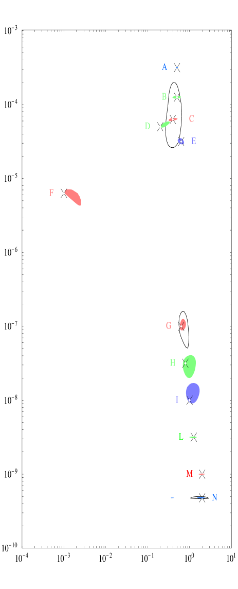
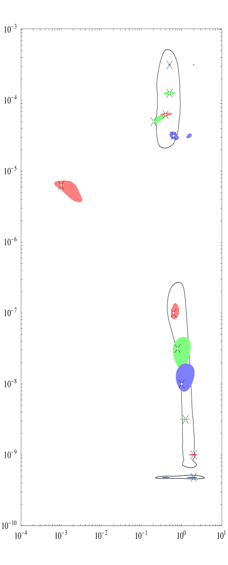
Figure 1: The continuous lines show the present global fit of solar data in the $(\tan^{2}\theta,\Delta m^{2}/\,{\rm eV}^{2})$ plane. The coloured regions are the simulated near-future fits (after KamLAND and Borexino) for few benchmark points, marked as $\times$ and listed in table 1. The left (right) plot shows fits at $90\%$ ($99\%$) confidence level. The true oscillation solution is identified in all cases (LMA, SMA, LOW, QVO, VO). Some simulated fits give very small regions: their main features can be read from table 1.

2 The near-future situation

We focus mainly on the oscillations of three active neutrinos, assuming that atmospheric oscillations do not affect solar neutrinos (in the standard notation, this amounts to have a large $\Delta m^{2}_{\rm atm}$ and a small $\theta_{13}$) because the relevant experiments [1, 2, 3, 4, 5, 6, 7, 12, 13, 14, 15, 16] (except LSND [17], see page 2) indicate that this is the physically relevant case. A three flavour analysis of solar (and atmospheric) data is no longer relevant [18]: reactor experiments [15] directly demand a small $\theta_{13}<15^{\circ}$ at $95\%$ CL, so that solar oscillations are presently determined by the usual two parameters, $\Delta m^{2}$ and $\theta.$

The continuous lines in fig. 1 show the present global fit [19, 20]. More or less acceptable fits can be obtained for a wide range of $\Delta m^{2}$ and for a large mixing angle. The best-fit solutions have $\chi^{2}_{\rm best}\approx 33$ from 41 experimental inputs and 2 free parameters; they lie in the LMA region, and have a $\Delta m^{2}$ around $10^{-4}\,{\rm eV}^{2}$. The other solutions with smaller $\Delta m^{2}$ (named LOW, QVO, VO) are not significantly worse: they poorly fit the data where a ‘solar anomaly’ is present, i.e. the total rates, but satisfy well the bounds from data consistent with no oscillations, i.e. spectral distortions, seasonal and day/night variations. However, the discrimination is not sharp: e.g., if GNO should decrease the central value of the Gallium counting rate down to $65\pm 5$ SNU, ($\sim 2\sigma$ below the present value), the global fit would favor the LOW solution.

In order to simplify the discussion it is useful to focus on few benchmark points that span the qualitatively different, still allowed solutions. These points (denoted as point A, B, C, …) are listed in table 1, and drawn as ‘$\times$’ in fig.  1. Some of them have a high $\Delta\chi^{2}\equiv\chi^{2}-\chi^{2}_{\rm best}$ (i.e. are significantly disfavoured, roughly at $(\Delta\chi^{2})^{1/2}$ standard deviations: for example there is a $\sim 7\sigma$ evidence for LMA versus no oscillations). We retained them in order to have a conservative sampling of all possible cases. The points D, M, N, O have a significantly lower $\Delta\chi^{2}$ in a solar-model-independent analysis, where the solar-model predictions for the Boron and Beryllium fluxes are not used (see [21] for a precise description).

Fig. 1 and table 1 illustrate the expected near-future achievements. In the last column of table 1 we summarize which sub-MeV measurements could provide us with further, useful information. When a certain sub-MeV measurement is crucial (not very interesting), we mark it by a ‘!’ (‘?’). While $\Delta m^{2}$ can be often measured very accurately, the determinations of $\theta$ may be less reliable. Indeed, the results on $\theta$ depend strongly on solar-model predictions; they could change e.g. if the Beryllium flux were lower than its predicted value. For points outside the LMA region, the error on $\theta$ (and consequently on $P_{ee}$) can be accurately estimated only after knowing the true results of near-future experiments, and could differ by a factor 2 from the values quoted in table 1.

The values of $\delta P_{ee}$ in the penultimate column of table 1 are the 1 standard-deviation, near-future uncertainty on the survival probability of the total $pp$ rate, as detected using $\nu_{e}e\to\nu^{\prime}_{e}e^{\prime}$ scattering, with electron kinetic energy larger than $T_{e^{\prime}}>0.1\,{\rm MeV}$ (taking into account the smaller $\nu_{\mu,\tau}$ NC cross section, the suppression in the total rate due to oscillations is roughly given by $0.8\ P_{ee}+0.2$). This quantity is important for sub-MeV experiments [10], since it informs us on how accurately those based on elastic scattering (as Heron, Clean, Xmass, Genius, Hellaz, etc.) should measure the $pp$ rate. Within the uncertainties, $\delta P_{ee}$ is also relevant for experiments based on inverse $\beta$-decay (as Lens, Moon, etc.).

One should recall that existing Gallium experiments are sensitive to $pp$ neutrinos (above $0.24\,{\rm MeV}$), that would induce half of their neutrino events in absence of oscillations. In the present perspective, we are lead to study how well the true rate of $pp$ neutrinos can be reconstructed from the total Gallium rate, after subtracting the values of the other fluxes (Boron, Beryllium, …)

$$R^{pp}_{\rm Ga}=R^{\rm total}_{\rm Ga}-R_{\rm Ga}^{\rm others}$$

as measured by the near-future (and present) experiments. Concerning the Boron flux, SK and SNO find that, within their accuracy, the survival probability of Boron neutrinos is energy-independent. Therefore, we directly use the Boron rate measured at SNO with $8.5\%$ error. The error on the Boron contribution to the Gallium rate is $\pm 1.5$ SNU, dominated by the $30\%$ uncertainty on its Gallium cross section [22].

Concerning the Beryllium and CNO fluxes, Borexino (and, maybe, KamLAND) should measure them. We assume that the error on Beryllium and CNO contributions to the total Gallium rate will again be dominated by the $\sim 10\%$ uncertainties on their Gallium cross section, so that the total error on $R_{\rm Ga}^{\rm others}$ will be $\pm 2$ SNU. We neglect the $pep$, $hep$ and F contributions, that are smaller than this error. The experimental error on $R^{\rm total}_{\rm Ga}$ is today $\pm 5$ SNU, and GNO should lower it down to $\pm(3\div 4)$ SNU. This means that the $pp$ rate will be known within $\pm(10\div 15)\%$ uncertainty, depending on its actual value (here, we assumed a large mixing angle). In this example, the average value of the survival probability for $pp$ neutrinos (around $0.5$) will be known with a $\pm 0.06$ uncertainty.

In the rest of the paper we motivate and discuss in detail the results summarized in table 1 and fig. 1.

LMA and EI

The present data favour the LMA region, and do not significantly disfavour energy independent (EI) solar oscillations, obtained for $\Delta m^{2}\,\raise 1.29167pt\hbox{$>$\kern-7.5pt\lower 4.30554pt\hbox{$\sim$}}\,2~{}10^{-4}\,{\rm eV}^{2}$ [23]. This region should be fully covered by the KamLAND experiment [8], which will detect reactor $\bar{\nu}_{e}$ using the reaction $\bar{\nu}_{e}p\to e^{+}n$. The accuracy of KamLAND has been discussed in [24, 21, 25, 26] and more importantly in [8]. As in [8] we assume (too conservatively?) that KamLAND will use a cut on visible energy $E_{e^{+}}+m_{e}>2.6\,{\rm MeV}$ (where $E_{e^{+}}=E_{\nu}-m_{n}+m_{p}$) in order to avoid the background due to ambient $\bar{\nu}_{e}$. We assume a rate of 550 events per year without oscillations, a $2\%$ overall uncertainty on the reactor flux and no background. The regions in fig. 1 surrounding the points B, C, D, E show how well KamLAND is expected to determine the oscillation parameters $\Delta m^{2}$ and $\theta,$ after three years of data-taking. The value of $\Delta m^{2}$ can be measured accurately because the initial spectrum is well known, and the energy resolution is sufficient to show the first oscillation dip.

However, if $\Delta m^{2}\,\raise 1.29167pt\hbox{$>$\kern-7.5pt\lower 4.30554pt\hbox{$\sim$}}\,2~{}10^{-4}\,{\rm eV}^{2}$ (the precise value depends on the energy resolution) KamLAND will only see averaged oscillations; thence, it will be unable to measure $\Delta m^{2}$ with good sensitivity [21]. Therefore, for point A we considered a new reactor experiment, with a baseline of $20\,\hbox{km},$ a rate of $3000$ events/year above $E_{e^{+}}+m_{e}>2.6\,{\rm MeV},$ and used three years of data for the estimate. This experiment has been named ‘sub-KamLAND’ in table 1 and in the following, because it is less demanding than KamLAND.

Despite the assumed $2\%$ uncertainty on the initial $\bar{\nu}_{e}$ flux, $P_{ee}$ (and consequently the mixing angle $\theta$) can be measured with an error less than $2\%$, if an oscillation signal is seen. In fact, the accuracy in the determination of $P_{ee}$ depends strongly on its value, being maximal when $\theta\sim\pi/4.$ It is possible to detect small deviations from maximal mixing. This can be understood in a qualitative way by considering an energy bin around the first oscillation dip, where $P_{ee}\sim 0$. It will contain a number of events $N_{\rm obs}$ much smaller than the no oscillation prediction, $N_{\rm O}$. Having assumed a negligible background, the survival probability in that bin can be measured with error $\delta P_{ee}\sim\sqrt{N_{\rm obs}}/N_{\rm O}$. This feature is more pronounced at the hypothetical sub-KamLAND than at KamLAND, where the $\bar{\nu}_{e}$ are produced by various reactors with different path-lengths, so that the first oscillation dip is partially averaged. (The situation would improve if KamLAND could reconstruct the direction of the neutrinos).

We now discuss how sub-MeV experiments could improve on this situation. Solar neutrinos with energy

$$E_{\nu}\,\raise 1.29167pt\hbox{$<$\kern-7.5pt\lower 4.30554pt\hbox{$\sim$}}\,\frac{\Delta m^{2}}{2\sqrt{2}G_{\rm F}N_{e}^{\odot}}\approx 1\,{\rm MeV}\frac{\Delta m^{2}}{10^{-5}\,{\rm eV}^{2}}$$ (1)

(where $N_{e}^{\odot}$ is the electron density around the region of neutrino production) do not experience the MSW resonance in the sun. Therefore, their oscillation probability is roughly given by averaged vacuum oscillations, $P_{ee}\approx 1-\frac{1}{2}\sin^{2}2\theta$. In first approximation, this implies that sub-MeV experiments have nothing to tell about $\Delta m^{2}$, but could give information on $\theta$. Note however that KamLAND will fix the value of $P_{ee}$ with an error less than $\pm 0.02,$ as shown in table 1. Though the precision of sub-MeV experiments is ultimately limited by the $1\%$ solar model uncertainty on the $pp$ flux, it seems unrealistic to aim at this level of accuracy, and even difficult to compete with KamLAND (or other upgraded reactor experiments). On the other hand, with a precise determination of $\Delta m^{2}$ and $\theta$ from a reactor experiment, sub-MeV experiments could be used to finally test solar model predictions, as suggested long time ago [28].

Reactor experiments can only measure $\sin^{2}(2\theta)$: the discrimination between $\theta$ and $\pi/2-\theta$ has to be performed by relying on matter effects acting on solar neutrinos. The present data prefer $\theta<\pi/4$, with a few standard deviations significance (its precise value depends on the actual value of $\theta$ and $\Delta m^{2}$ [26]). Which new experiments are best suited for this issue? Neutrino fluxes are better known at lower $E_{\nu}$, but in the LMA region matter effects are larger at $E_{\nu}\sim 10\,{\rm MeV}$ than at $E_{\nu}\,\raise 1.29167pt\hbox{$<$\kern-7.5pt\lower 4.30554pt\hbox{$\sim$}}\,\,{\rm MeV}$. At larger $E_{\nu},$ the uncertainty on the Boron flux can be circumvented by the NC and CC measurements at SNO (and SK). The NC/CC ratio today prefers $\theta<\pi/4$ at $\sim 1.5$ standard deviations, and could provide a direct discrimination in the near future. If $\Delta m^{2}$ is in the lower part of the LMA region, earth matter effects at SK and SNO [29] could discriminate $\theta$ from $\pi/2-\theta$. Matter corrections to the spectrum of $\bar{\nu}_{e}$ from a future supernova should also give a clear discrimination: unlike $\nu_{e}$, $\bar{\nu}_{e}$ cross a resonance if $\theta>\pi/4$.

LOW

The most promising LOW signals in near-future experiments are earth matter effects at Borexino and, maybe, at KamLAND [8, 30]. In fact, after having excluded the LMA region, KamLAND could be converted into a solar neutrino experiment. In absence of oscillations, Borexino (KamLAND) is expected to have a signal rate of 59 (280) events/day for the central value of the Beryllium, CNO, $pep$ fluxes predicted by [31] and a background rate of 19 (130) events/day, known with $\delta b=10\%$ ($50\%$) error. Even if the background were more uncertain, the seasonal variation of the solar neutrino flux (due to the excentricity of the earth orbit) would allow a measurement of the signal rate with an interesting accuracy [8, 30]. We concentrate on Borexino and consider only the signal due to the Beryllium line (46 events/day), after three years of running.

At present, it is not clear if it will be possible to measure the CNO and $pep$ contributions, using a sufficiently background-free energy region above the Beryllium line. A pessimistic attitude would require to assume that it will be only possible to use those events with recoil $e$ energy between $0.25$ and $0.8\,{\rm MeV}$, generated by Beryllium (46 events/day), CNO (10 events/day), $pep$ (2 events day) neutrinos [9] plus of course the background. However, we remark that this possible limitation would be a problem to test of solar models, but would have just a little effect on the determination of $\Delta m^{2}$ and $\theta$.

We perform our analysis along the lines of [30], but paying more attention to the determination of the oscillation parameters, rather than to the discovery of oscillation signals. We divide the simulated data into $N_{\rm bins}=8+1$ zenith bins (8 night zenith bins equally spaced in $\cos\theta_{\rm zenith}$, plus one day bin) and define

$$\chi^{2} = \sum_{i=1}^{\rm N_{\rm bins}}\frac{(N_{i}-S_{i}-bB_{i})^{2}}{N_{i}}+$$

$$+\bigg{(}\frac{\Phi_{{}^{7}{\rm Be}}-\Phi^{\rm BP}_{{}^{7}{\rm Be}}}{\delta\Phi^{\rm BP}_{{}^{7}{\rm Be}}}\bigg{)}^{2}+\frac{(b-1)^{2}}{\delta b^{2}},$$

where $N_{i}$ is the measured number of events; $S_{i}$ is the expected number of signal events (proportional to $P_{ee}$ and to the solar flux $\Phi_{{}^{7}{\rm Be}}$); $bB_{i}$ is the expected number of background events (the factor $b$ takes into account the overall uncertainty on the background rate). Finally the $\chi^{2}$ in eq. (2) is added to the $\chi^{2}$ from present data, properly taking into account the correlation of the theoretical uncertainties on the Beryllium flux [31, 22]. A $\chi^{2}$ as in eq. (2), when minimized with respect to the ‘nuisance’ unknown parameters (here $b$ and $\Phi_{{}^{7}{\rm Be}}$; more generically the solar-model parameters and the detection cross sections) gives the same $\chi^{2}$ defined in [22], where all uncertainties are summed in quadrature, obtaining a big error matrix.

The simulated fit for point G (which gives the best-fit in the LOW region) is similar to the corresponding result in fig. 6 of [30] (where KamLAND instead of Borexino was considered). The accuracy is worse at point H, because earth matter effects diminish with $\Delta m^{2}$. We do not show simulated fits for points located around the highest $\Delta m^{2}$ values allowed in the LOW region (that will be soon tested by SNO and are already directly disfavoured by the non-observation of a day/night asymmetry at SK and Gallex/SAGE/GNO [33]): due to the large earth matter effects, the accuracy on the determination of $\Delta m^{2}$ would be so good that one should carefully take into account the uncertainty in the profile density of the earth (while this is not an issue for the points that we have selected).

The survival probability of sub-MeV neutrinos is given by adiabatic conversion: $P_{ee}=\sin^{2}\theta$ during the day. An accurate measurement of the $pp$ rate would provide the safest determination of $\theta$, because solar-model predictions will play little rôle. It will be interesting to perform this measurement even if present and near-future experiments will nominally give a somewhat more accurate determination of $\theta$.

Furthermore, earth matter effects give a day/night variation of the $pp$ rate, allowing to measure also $\Delta m^{2}$. However, even if matter effects are larger at $pp$ energies than at higher energy, it is more convenient to study $\Delta m^{2},\theta$ at Borexino (KamLAND, or new experiments based on inverse $\beta$-decay) due to the monochromaticity of Beryllium neutrinos and to the larger event rate.

LOW/QVO boundary

We pragmatically define the boundary between the LOW and QVO regions [34] as

$$\Delta m^{2}({\rm LOW})\ \,\raise 1.29167pt\hbox{$>$\kern-7.5pt\lower 4.30554pt\hbox{$\sim$}}\,\ 10^{-8}\,{\rm eV}^{2}\ \,\raise 1.29167pt\hbox{$>$\kern-7.5pt\lower 4.30554pt\hbox{$\sim$}}\,\ \Delta m^{2}({\rm QVO})$$

because this is the critical $\Delta m^{2}$ under which Borexino (KamLAND) should observe anomalous seasonal effects (see e.g. [8, 35, 32]), rather than the day/night effects characteristic of the LOW region (see e.g. [8, 30]). The regions considered in the rest of this paper will be soon disfavoured, if SNO finds a day/night asymmetry.

No unmistakable signal of solar neutrino oscillations can be observed by near-future experiments if $\Delta m^{2}$ lies around this critical value. In view of this situation, we tried to exploit, in this particular point, the full capability of near-future experiments by optimistically assuming that KamLAND will be converted into a solar neutrino experiment as described above. KamLAND would detect a hint of day/night effect, giving some information on $\Delta m^{2}$. Borexino (and existing data) would provide instead the dominant information on $\theta$. By combining these pieces of information, we obtain the simulated fit for point I.

Though the near-future uncertainty in $\Delta m^{2}$ is significantly smaller than the present uncertainty, it remains rather big. It should be understood that the improvement is mainly due to the fact that all other regions with larger and smaller $\Delta m^{2}$ will be firmly excluded, because they predict unobserved clear signals. To prove this, we omitted the only positive signal (attributed to KamLAND) and obtained roughly the same $\Delta m^{2}$ interval.

A measurement of the $pp$ rate could give additional informations on $\theta$. However a measurement of $\Delta m^{2}$ resulting from a global fit may be felt as unsatisfactory. As discussed in the ‘no oscillations’ section, the detection of Beryllium neutrinos would ensure that a solar neutrino anomaly is present, but we would still not know if it is due to oscillations. A sub-MeV experiment could discover an unmistakable oscillation signal: the neutrino energy at which earth matter effects induce a maximal day/night asymmetry is

$$E_{\nu}^{\rm res}=\frac{\Delta m^{2}}{2\sqrt{2}G_{\rm F}N_{e}^{\oplus}}\approx\frac{\,{\rm MeV}}{40}\frac{\Delta m^{2}}{10^{-8}\,{\rm eV}^{2}},$$

where $N_{e}^{\oplus}$ is the electron density of the earth mantle. Because of the low value of $E_{\nu}^{\rm res}$, one would need a big real-time detector, with an energy threshold as low as possible in order to detect this effect.

However, at a detector with a threshold $T_{e}>0.1$ MeV (such as Heron, Clean, Xmass, Genius, Hellaz etc.) the day/night asymmetry at point I (a $\sim 4$ % excess in nighttime) is only twice larger than at Borexino or KamLAND, that could instead have many more events. A very low threshold, maybe as low as 11 keV, could be attained by the Genius experiment with a rate of 18 $pp$ events/day (assuming a mass of 10 ton). However only few $\%$ of the $pp$ neutrinos have energy below $0.1\,{\rm MeV},$ and they cannot be individually identified by the elastic scattering reaction.

QVO

The distance between the earth and the sun varies as

$$L(t)=L_{0}[1-\epsilon\cos(2\pi t/{\rm yr})+{\cal O}(\epsilon^{2})]$$

where $L_{0}=1.496~{}10^{8}\,\hbox{km}$ is the astronomical unit, $\epsilon=0.0167$ is the excentricity of the earth orbit, and $t$ is the time since the perihelion (around $4{\rm th}$ of January). This variation induces a modulation of the survival probability in QVO and VO regions, that can be investigated at Borexino, and eventually at KamLAND, by means of the almost mono-energetic Beryllium neutrinos, $E_{{}^{7}{\rm Be}}=0.863\,{\rm MeV}$ [35, 32].

The time variation of the survival probability is [34]

$$P_{ee}(t)=\langle P_{ee}\rangle+\sin 2\theta\sqrt{P_{C}(1-P_{C})}D\cos(kL(t)+\delta),$$

where $k={\Delta m^{2}}/{2E_{{}^{7}{\rm Be}}}$ and $\delta\sim 0.13\,kR_{\odot}$ [34]. The number of oscillations met in one semester can be large (fig. 2):

$$N_{\rm osc}=\frac{\epsilon L_{0}\Delta m^{2}}{2\pi E_{{}^{7}{\rm Be}}}\approx\frac{\Delta m^{2}}{0.85~{}10^{-9}\,{\rm eV}^{2}}.$$ (3)

These oscillations get washed for increasing $\Delta m^{2},$ due to the MSW effects inside the sun (taken into account by the crossing-probability factors $P_{C}$) and to the finite width of the Be line (taken into account by the factor $D$, given by the Fourier transform [34] of the Beryllium ‘line’ spectrum [36]), as illustrated in fig. 2.

We perform the simulated fits using a $\chi^{2}$ with a large number of seasonal bins: $N_{\rm bins}\sim 10\cdot N_{\rm osc}.$ Of course, $N_{\rm osc}$ is a priori unknown in actual analyses, and should be extracted from the data; a definition of $\chi^{2}$ that avoids this problem, and allows to exploit all the data is discussed in Appendix A. Anyhow, our conclusion is that $\Delta m^{2}$ can be measured with surprisingly good precision (see table 1, or enlarge fig. 1). The point is that when the number of oscillations $N_{\rm osc}$ is big, Borexino acts as an interferometer.

Figure 2: Number $N_{\rm osc}$ and amplitude $a$ of seasonal oscillations as function of $\Delta m^{2}$ in $\,{\rm eV}^{2}$ for $\tan^{2}\theta=\{1/\sqrt{10},1,\sqrt{10}\}$ (long dashed, dotted, dashed).

These results can be understood by a simple analytical estimate. First, we display in fig. 3 the signal as a function of time, for the benchmark points I, L and M. The number of events at Borexino can be written as:

$$N\propto 1+a\cos(kL+\delta).$$ (4)

considering the events due to Beryllium neutrinos (CC and NC) and the estimated background, and omitting the geometrical $1/L^{2}$ flux factor. The amplitude of oscillations $a$ is plotted in fig. 2, for three choices of the mixing angles. The average value of $N$ during the time periods with $\cos(kL+\delta)>0$ ($<0)$ is $N_{\pm}\propto 1\pm 2a/\pi$. Thence, one gets an “asymmetry” (systematic excess) of events:

$$\frac{4a}{\pi}=\frac{N_{+}-N_{-}}{(N_{+}+N_{-})/2}\pm\sqrt{\frac{2}{N_{+}+N_{-}}}.$$

The error on $a$ can be small even if $N_{\rm osc}$ is big:

$$\delta a=\frac{\pi}{4}\sqrt{\frac{2}{N_{+}+N_{-}}}=0.005\sqrt{\frac{50000}{N_{+}+N_{-}}}.$$

The ‘seasonal’ oscillation is detected if the amplitude $a$ is sufficiently larger than its uncertainty $\delta a$, and this happens if $\Delta m^{2}\,\raise 1.29167pt\hbox{$<$\kern-7.5pt\lower 4.30554pt\hbox{$\sim$}}\,0.5~{}10^{-8}\,{\rm eV}^{2}.$ Values of $\theta<\pi/4$ are more suitable; see again fig. 2.

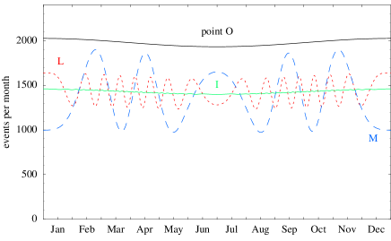
Figure 3: Seasonal variation of the signal at Borexino for the benchmark points. The upper line is the no-oscillation case.

Once a seasonal signal is seen with $N_{\sigma}=a/\delta a$ standard-deviations, the number of oscillations $N_{\rm osc}$ can be measured with an error $\delta N_{\rm osc}\approx 1/2N_{\sigma}$ that does not depend on $N_{\rm osc}$. Using eq. (3), the consequent error on $\Delta m^{2}$ is

$$\frac{\delta\,\Delta m^{2}}{\Delta m^{2}}=\frac{\delta N_{\rm osc}}{N_{\rm osc}}=\frac{1}{2N_{\sigma}N_{\rm osc}}\qquad\hbox{if $N_{\sigma}>$ few}.$$ (5)

For example, from fig. 2 we can read that in point L $N_{\rm osc}\sim 7$ and $N_{\sigma}\sim 20$. This explains why in table 1 we claim an extremely accurate measurement of $\Delta m^{2}$. The analytical approximation tells how our numerical results should be rescaled in order to extend our analysis to KamLAND or to a longer data-taking period. For example, with 9 times more signal, $\delta a$ would be 3 times smaller, giving a per-mille determination of $\Delta m^{2}$. The accuracy is limited by statistics (and by the small excentricity of the earth orbit). No knowledge of the Beryllium spectrum or of other solar-model dependent features is required.

The overall phase in $\cos(kL_{0}+\delta)$ depends on the total earth-sun distance (rather than on its excentricity variation) and is therefore more strongly dependent on $\Delta m^{2}$. It contains additional information: it separates the allowed region of $\Delta m^{2}$ into $\delta N_{\rm osc}/2\epsilon\approx\hbox{few}$ separate thin islands [32]. We do not include this information in our fits: the error or $\Delta m^{2}$ is already so small that it would not even be possible to see this sub-structure in fig. 1.

Beryllium neutrinos contribution is $\sim 30\%$ of the total rate measured at SAGE and Gallex/GNO. These experiments are further limited by a modest time resolution, $\Delta t\sim\hbox{weeks},$ and thence their sensitivity to seasonal variations is reduced. No such a signal has been found, which implies weak bounds on the oscillation parameters [37], usually neglected in global analyses.

Subsequent $pp$ experiments cannot improve on this determination of $\Delta m^{2}$. A measurement of the $pp$ rate would instead give a useful information on the mixing angle. However, this information would have a certain degree of solar-model dependence. Indeed, in the QVO region the survival probability $\langle P_{ee}\rangle=\frac{1}{2}+(P_{C}-\frac{1}{2})\cos 2\theta$ lies somewhere between vacuum oscillations ($\langle P_{ee}\rangle=1-\frac{1}{2}\sin^{2}2\theta$ for $P_{C}=\cos^{2}\theta$) and adiabatic oscillations ($\langle P_{ee}\rangle=\sin^{2}\theta$ for $P_{C}=0$), as controlled by the crossing-probability $P_{C}=[e^{\gamma\cos^{2}\theta}-1]/[e^{\gamma}-1]$ where [38]

$$\gamma=\frac{\pi\Delta m^{2}}{E_{\nu}|d\ln N_{e}/dr|_{\rm res}}\approx\frac{\Delta m^{2}/E_{\nu}}{10^{-9}\,{\rm eV}^{2}/\,{\rm MeV}}.$$

The gradient is evaluated around the resonance point (for a more accurate approximation see [34]) where the density is $N_{e}\sim\Delta m^{2}/G_{F}E_{\nu}$: this corresponds to the outer part of the sun where the profile density deviates from the simple exponential approximation, $N_{e}\propto\exp(-10.54\,r/R_{\rm sun})$.

Before concluding, we recall that an accurate treatment of CNO and $pep$ neutrinos would require to know the actual performance of the near-future detectors. However, the sensitivity of the determination of $\Delta m^{2}$ through Beryllium neutrinos would be not substantially affected, even in the most pessimistic case. Instead, in the most optimistic case, $pep$ neutrinos could give an additional modulated signal with frequency $k_{pep}\approx 0.6k$ and amplitude $a_{pep}\sim a/10,$ referred to those of Beryllium neutrinos, eq. (4). Since the $pep$ flux is well known, almost as the $pp$ flux, $a_{pep}$ could yield information on $\theta$.

VO

Vacuum oscillations offer the same seasonal signal as discussed in the previous section. Solar matter effects can now be neglected, so that the energy-averaged survival probability is $\langle P_{ee}\rangle=1-\frac{1}{2}\sin^{2}2\theta$. The number of seasonal vacuum oscillations $N_{\rm osc}$ encountered during one semester is smaller, so that the accuracy in $\Delta m^{2}$ is somewhat worse (see eq. (5)), but remains much better than sub-MeV capabilities. A measurement of the $pp$ rate would give a solar-model independent information on the mixing angle. Some vacuum oscillation ‘solutions’, usually named “Just So²”, that give poor fits of existing data present characteristic spectral distortions in $pp$ neutrinos [39]. Our point N gives a rather good fit to the data. In fact, the Beryllium line is affected by seasonal effects (while the other fluxes are less affected due to their larger energy spread) in a way that very strongly depends on $\Delta m^{2}$: choosing the appropriate value one can obtain the experimentally preferred value of the Beryllium rate.

SMA

The SMA region is strongly disfavoured by existing experiments and has a low goodness-of-fit. The reason is that the SMA oscillations that fit the measured rates imply a survival probability $P_{ee}(E_{\nu})$ in conflict with the SK spectral data. This conflict can be seen in pre-SNO fits performed by the SK collaboration [5] and has become sharper after SNO. Our SMA point, F, is not the ‘best’ current SMA solution (that has $\Delta\chi^{2}\approx 14$, similar to [19, 20]) but a representative point of this region. In view of this situation, it is difficult to study seriously how well new experiments can measure $\Delta m^{2}$ and $\theta$ in the SMA region.

The most characteristic feature of the SMA region is that

• the neutrino rate at Borexino will be strongly suppressed (almost down to the background level).

Depending on the actual SMA oscillation, this evidence for SMA can be stronger than the present evidence against SMA. In this situation one could doubt that Borexino will be able to detect solar neutrinos at all. Therefore we also assume that

• SNO will see a distortion of the spectrum, and will contradict the SK spectral data.

Assumptions 1 and 2 imply a very bad goodness-of-fit. A good SMA fit could be obtained if the SK collaboration would commit hara-kiri, admitting:

• serious faults in the SK solar neutrino results.

In this case, we would be authorized to drop the the SK spectral data from the global fit. Under these three assumptions, we obtain the SMA future fit in fig. 1. Borexino data select the SMA region over the other ones, but without favouring any particular corner there; this selection is done by the other data, that prefer the region of large $\theta$. We can consider a different possibility: if the CC rate measured at SNO is wrong (so that we drop it from the $\chi^{2}$), but the SK spectral data are correct, the SMA range with small $\theta$ would be selected. Incidentally, this tension between the preferred $\theta$ range reflects once again the tension between the data, once we assume SMA.

In any case, if something like this were to happen, we would certainly need new experiments to confirm it. The $pp$ rate should be consistent with no oscillation, because SMA predicts $P_{ee}\approx 1$ at very low energy. In order to make the solar neutrino anomaly credible, we would need to have a spectral measurement at low energy, aimed at revealing the sharp SMA transition from $P_{ee}\approx 1$ to $P_{ee}\approx 0,$ for energies around the value in eq. (1).

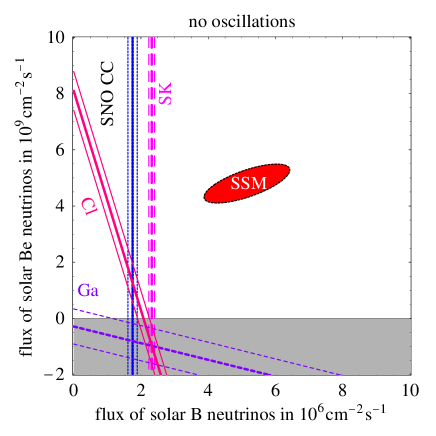
Figure 4: Values of the Boron and Beryllium fluxes required at $1\sigma$ by the four measured solar neutrino rates in absence of oscillations, compared to the $68\%$ C.L. ellipse of solar model predictions.

No oscillations

The hypothesis of no oscillations can be reconciled with the data if the Boron and Beryllium fluxes are very different (smaller) from solar model predictions, as shown in fig. 4; see [21] and ref.s therein. Even in this case, the rates measured by the various experiments are not well compatible between them. But, as shown in fig. 4, there is a significant (accidental?), partial overlap of the experimental values. This is why solar-model independent considerations cannot strongly disfavour the no-oscillations hypothesis — whereas generically such accident does not happen and useful solar-model-independent information can be deduced already from existing data [21].

The zero Beryllium flux required by no oscillations is disfavoured by helioseismology [40], by simple physics considerations, and by recent results. Indeed, solar models [31] have been recently validated by two facts. The determination of $S_{17}$ (strength of the $p{}^{7}{\rm Be}\to{}^{8}{\rm B}\gamma$ reaction) has been improved [41, 42], and as a consequence the correlation between the flux of Boron and Beryllium neutrinos, visible in fig. 4, will tighten (both neutrino fluxes are controlled by the $\alpha{}^{3}{\rm He}\to{}^{7}{\rm Be}\gamma$ reactions; thence the relative $S_{34}$-factor remains the dominant, common source of uncertainty). Furthermore, the SNO/SK measurement of the Boron flux [7], is in agreement with the solar-model prediction, within the $\sim 20$ % error. These two facts suggest that the calculated Beryllium flux should not be too wrong. Certainly, the solar model independent considerations will become cogent after the Borexino measurement of the Beryllium flux.

Since the prediction of the $pp$ flux is very accurate [31] $\Phi_{pp}=(5.96\pm 1\%)10^{10}/\hbox{cm}^{2}\hbox{s},$ its determinations will also have an important impact on these analyses. Indeed, a well known simple (though, less accurate) argument leads to the same value of the flux. We assume that the solar energy comes from nuclear reactions that reach completion, and that the sun is essentially static over the time employed by photons to reach the surface. The total luminosity of the sun, $K_{\odot}=8.53\cdot 10^{11}$ MeV cm^-2 s^-1 at the earth, determines its total neutrino luminosity as $K_{\odot}=\sum_{\alpha}\left({Q}/{2}-\langle E_{\nu_{\alpha}}\rangle\right)\Phi_{\alpha};$ $Q=26.73$ MeV is the energy released in the reaction $4p+2e\rightarrow\,^{4}\!{\rm He}+2\nu_{e},$ and the sum extends over the various components ($\alpha=pp,pep,\rm^{7}\!Be,^{13}\!N,^{15}\!O,{}^{17}\!F,{}^{8}\!B,h\hbox{$ep$}$). Neglecting $\langle E_{\nu_{\alpha}}\rangle$ and considering only the dominant $pp$ flux, one obtains $\Phi_{pp}\approx 2K_{\odot}/Q=6.4\cdot 10^{10}/\hbox{cm}^{2}\hbox{s}$, that is only $7\%$ off. Therefore, a measurement of the $pp$ rate, even with modest accuracy, will provide strong solar-model-independent evidence against (or for) the extreme possibility of no oscillations.

Sterile neutrinos

The LSND anomaly can be used to argue for additional sterile neutrino(s); however, the evidence against such neutrino(s) is now stronger than the evidence for them. For example, the ‘2+2’ best solution found in [43] where LSND is explained has a worse global fit than the 3-neutrino solution where it is not (and consequently than the best ‘3+1’ solutions, where the sterile neutrino is of little use for LSND [44]). Indeed, the relevant global $\chi^{2}$ is:

$$\chi^{2}_{\rm global}=\chi^{2}_{\rm sun}+\chi^{2}_{\rm atm}+\chi^{2}_{\rm LSND}.$$

Using one sterile neutrino, the best fit gives [43]

$$\chi^{2}_{\rm global}=40+36+0=76\qquad\hbox{with 9 parameters.}$$

Without using the sterile neutrino, the $\chi^{2}$ is [43]

$$\chi^{2}_{\rm global}=37+29+10=76\qquad\hbox{with 5 parameters.}$$

CP-violating phases are not counted as relevant parameters. The $\chi^{2}_{\rm global}$ of [43] does not take into account data from SNO; from Karmen; from nucleosynthesis; from unpublished atmospheric SK data about the total $\pi^{0}$ rate (and recent K2K cross section determinations) and about their zenith angle dependence [45]. Each one of these data further disfavours the best-fit ‘2+2’ solution of [43], which has a large sterile component in atmospheric oscillations. From a theoretical point of view, ‘2+2’ schemes need a very special arrangement of mixing angles. This pattern can be obtained from a ‘pseudo-Dirac’ mass matrix, which can be justified by a broken U(1) $L_{\mu}-L_{\tau}-L_{s}$ symmetry, and implies quasi-maximal mixing in atmospheric oscillations.

If MiniBoone will confirm LSND, it will be interesting to consider solar oscillations into a mixed sterile/active neutrino. What would be the impact on the present analysis? The near-future prospects concerning the determination of the solar parameters $\theta$ and $\Delta m^{2}$ are almost unchanged. This is an exact statement in the LMA region, since KamLAND cannot distinguish if reactor $\bar{\nu}_{e}$ disappear into active or sterile antineutrinos. The most relevant new issue is that solar oscillations would depend on a third parameter (other than $\Delta m^{2}$ and $\theta$), that quantifies the sterile component in solar oscillations (for a precise definition, see e.g. [43]). In this case, it would be interesting to supplement the NC/CC measurement of the Boron flux performed at SNO and SK with a NC/CC measurement of the $pp$ flux, because it is accurately predicted by solar models. Furthermore, it could be convenient to obtain a CC measurement of the Beryllium flux, which could be combined with the result of Borexino (KamLAND).

3 Summary

In the near future KamLAND or Borexino should identify the true solution of the solar neutrino problem, if it is due to oscillations. Depending on the actual value of the oscillation parameters $\Delta m^{2}$ and $\theta$, the future situation will be very different, and will correspondingly require different new experiments. We summarize the various possibilities below (see the text for a more detailed discussion):

• LMA. KamLAND or sub-KamLAND will measure $\Delta m^{2}$ with few per-cent accuracy. Even the mixing angle $\theta$ can be determined reasonably well by reactor experiments; it will be a real challenge for sub-MeV experiment to improve on these measurements.

• LOW. Borexino will see day/night effects and measure $\Delta m^{2}$ with $10\%$ accuracy. A measurement of the $pp$ rate would be useful for determining $\theta$ and a measurement of day/night effects in $pp$ neutrinos could help in determining $\Delta m^{2}$.

• LOW/QVO boundary. No unmistakable oscillation effect will be found, but all other solutions will be excluded. A measurement of day/night effects (that are largest for the lowest-energy $pp$ neutrinos) would be crucial.

• QVO and VO. Borexino will see seasonal effects and measure $\Delta m^{2}$ with few per-mille accuracy, that can be improved with more statistics. A measurement of the $pp$ rate would be useful.

We comment also on strongly disfavoured possibilities, that could strike back again, if near-future experiments will contradict some combination of established data:

• SMA. Will become again the best solution if Borexino finds almost no solar neutrinos (because all Beryllium $\nu_{e}$ get converted); one has to assume e.g. that the SK spectral data are not correct. A spectral measurement around $E_{\nu}\sim\,{\rm MeV}$ would provide a crucial signal.

• No oscillations. Could become the ‘best’ solution if Borexino finds no solar neutrinos (because the Beryllium flux is much smaller than what solar models and helioseismology tell us — this possibility looks very remote) and if the CC/NC rate measured at SNO/SK is incorrect. The measurement of the $pp$ rate would be of essential importance.

• Just So². Will become the best solution if the CC/NC rate measured at SNO/SK will change (contradicting present data) indicating no oscillation, and if Borexino will find a somewhat suppressed flux of Beryllium neutrinos. A measurement of the $pp$ spectrum would be crucial.

Near-future experiments will allow us to deduce the $pp$ flux from GNO data, without assuming oscillations or using solar model predictions, with $\,\raise 1.29167pt\hbox{$<$\kern-7.5pt\lower 4.30554pt\hbox{$\sim$}}\,15\%$ uncertainty.

Acknowledgments

We thank E. Bellotti, C. Cattadori, N. Ferrari A. de Gouvêa, A. Ianni, M. Junker and S. Schönert for useful discussions.

Appendix A A seasonal $\chi^{2}$ for Borexino

The standard procedure employs a certain number $N_{\rm bins}$ of seasonal bins and a $\chi^{2}$ analogous to the one defined in eq. (2) for the day/night analysis. As is apparent from fig. 2, the appropriate number of seasonal bins is proportional to the unknown value of $\Delta m^{2}$, and many seasonal bins are necessary when $\Delta m^{2}\,\raise 1.29167pt\hbox{$<$\kern-7.5pt\lower 4.30554pt\hbox{$\sim$}}\,10^{-8}\,{\rm eV}^{2}$ because $N_{\rm osc}$ is large. However, eq. (2) cannot be applied if the number of events in each bin is not much larger than 1. In this situation, one should not employ Gaussian statistics; instead, the likelihood of the given measurement, given the oscillation parameters reads:

$$e^{-{\chi^{2}}/{2}}=\prod_{i=1}^{N_{\rm bins}}\frac{\epsilon_{i}^{n_{i}}}{n_{i}!}e^{-\epsilon_{i}},$$

where the individual factors are the Poisson probabilities of having $n_{i}$ observed events in the $i^{th}$ bin, in which $\epsilon_{i}$ events are expected. This $\chi^{2}$ function can be written as:

$$\chi^{2}=2N_{\rm th}-2\sum_{m}m\sum_{i_{m}=1}^{N_{m}}\log\epsilon_{i_{m}}+{\rm const,}$$

where $N_{\rm th}$ denotes the total number of expected events and the index $i_{m}$ runs over the $N_{m}$ bins with $m=\{1,2,\ldots\}$ observed events, so that $N_{0}+N_{1}+N_{2}+\ldots=N_{\rm bins}$.

Poisson statistics simplifies in the limit of a very large number of seasonal bins (e.g. 1 bin per millisecond), so that $\epsilon_{i}\ll 1$. In this situation there are only bins with 0 or 1 measured events, so that $N_{0}+N_{1}=N_{\rm bins}$ and

$$\chi^{2}=2N_{\rm th}-2\sum_{i=1}^{N_{1}}\log\epsilon_{i}$$ (6)

If $N_{\rm osc}$ were large, this $\chi^{2}$ may be useful to perform a seasonal analysis at Borexino, already after the first 6 months of data.

We compare our $\chi^{2}$ with other approaches. A standard Fourier-transform analysis of Borexino seasonal data has been suggested in [35]. Equation (6) is, essentially, a non-standard type of transform, performed with respect to the event rate predicted by oscillations, rather than to the standard Fourier basis of ‘$\sin$’ and ‘$\cos$’ functions. This non standard choice minimizes the uncertainty on $\theta$ and $\Delta m^{2}$. A similar idea has been proposed in [46] (where a rough approximation to the spectrum of Beryllium neutrinos has been employed) but its statistical meaning is not clear. Systematic and theorethical uncertainties can be easily taken into account, by writing the expected number of events as a function of ‘nuisance’ unknown parameters, in analogy with eq. (2). Our definition of the $\chi^{2}$ is essentially the same as those employed in analyses of the SN 1987A data [47].

Appendix B Details of the computation

Unfortunately, fitting solar neutrino data is a subtle issue: In order to perform inferences on the parameters of oscillation, one has to merge together many pieces of data and information (nuclear physics, solar models, matter effects in the sun and in the earth, various experiments, …). We used information from many papers [1, 3, 4, 5, 6, 7, 31, 15, 22, 34, 48, 38, 49, 50, 51, 52, 53]. It is briefer to list here what is not included in our fit. Most of the other global fits have similar shortcomings.

The spectrum of recoil electrons in SK and SNO is computed in the simplest approximation (e.g. neither one-loop effects nor photon emission [54] are included). One-loop corrections to the MSW effect are neglected. Seasonal Gallex/GNO and SAGE data are not included. The treatment of solar matter effects in the QVO region is not as precise as in [34]. When computing confidence levels, we approximate $e^{-\chi^{2}/2}$ with a Gaussian function of $\Delta m^{2}$ and $\theta$: correct frequentistic and Bayesian analyses [20] do not give a significantly different result. All above issues do not have significant effects. Alternative possible definitions of the $\chi^{2}$ give $\Delta\chi^{2}$ values similar to those quoted in table 1. Note that the first digit of the $\Delta\chi^{2}$ is significant.

Our fit of SK data is based on table III of [5]. It only allows us to reproduce the total rate and the total day/night asymmetry (quoted in [5]) with $\sim 1\sigma$ accuracy. This small discrepancy is presumably due to the fact that the $\chi^{2}$ used by the SK collaboration includes a proper treatment of data about the background, so that the total rate is not the sum of the rates in each energy bin: the bins with higher energy are relatively more important, since they have less background.

References

- [1] The results of the Homestake experiment are reported in B.T. Cleveland et al., Astrophys. J. 496 (1998) 505.
- [2] The Kamiokande collaboration, Phys. Rev. Lett. 77 (1996) 1683.
- [3] The Gallex collaboration, Phys. Lett. B447 (1999) 127.
- [4] The SAGE collaboration, Phys. Rev. C60 (1999) 055801.
- [5] The SuperKamiokande collaboration, hep-ex/0103032. Its published version does not contain table III, which gives the real data employed in out fit. See also the SuperKamiokande collaboration, hep-ex/0103033.
- [6] The GNO collaboration, Phys. Lett. B490 (2000) 16.
- [7] The SNO collaboration, nucl-ex/0106015.
- [8] K. Inoue (for the KamLAND collaboration), talk at the Gran Sasso conference, 12–14 March 2001, page 429; “Proposal for USA participation in KamLAND”, available at kamland.lbl.gov.
- [9] The Borexino web page, almime.mi.infn.it/html/borexinof.html. See also B. Caccianiga (for the Borexino collaboration), talk at the Vanderbilt conference (5–10 March 2001).
- [10] For an updated review, see the talk of S. Schönert at TAUP 2001 “Solar and Reactor Neutrinos: Upcoming Experiments and Future Projects”, LNGS, 8-12 Sept, 2001, web page http://taup2001.lngs.infn.it/.
- [11] J.M. Williams, physics/0007078, version 21.
- [12] The SuperKamiokande collaboration, Phys. Rev. Lett. 85 (2000) 3999 (hep-ex/0009001).
- [13] The MACRO collaboration, Phys. Lett. B517 (2001) 59 (hep-ex/0106049); T. Montaruli, M. Sioli, M. Spurio for the MACRO collaboration, Proc. of ICRC, Hamburg, Aug 7-15, 2001.
- [14] The Bugey collaboration, Nucl. Phys. B434 (1995) 503.
- [15] The Chooz collaboration, Phys. Lett. B466 (1999) 415 (hep-ex/9907037); see also the Palo Verde collaboration, Phys. Rev. Lett. 84 (2000) 3764 (hep-ex/9912050). For a review on reactor experiments, see C. Bemporad, G. Gratta, P. Vogel, hep-ph/0107277.
- [16] The Karmen collaboration, Nucl. Phys. Proc. Suppl. 91 (2000) 191 (hep-ex/0008002).
- [17] The LSND collaboration, hep-ex/0104049.
- [18] For three-flavour analyses of solar and atmospheric data made obsolete by the CHOOZ data see e.g. G.L. Fogli, E. Lisi, D. Montanino, Astropart. Phys. 4 (1995) 177; R. Barbieri et al., JHEP 12 (1998) 017 (hep-ph/9807235).
- [19] G.L. Fogli, E. Lisi, D. Montanino, A. Palazzo, hep-ph/0106247; J.N. Bahcall, M.C. Gonzalez-Garcia, C. Peña-Garay, hep-ph/0106258; A. Bandyopadhyay, S. Choubey, S. Goswami, K. Kar, hep-ph/0106264; the SNO-updated version of [20]; P.I. Krastev and A. Yu Smirnov, hep-ph/0108177.
- [20] P. Creminelli, G. Signorelli and A. Strumia, JHEP 0105 (2001) 52 (hep-ph/0102234, updated version).
- [21] R. Barbieri, A. Strumia, JHEP 0012 (016) 2000 (hep-ph/0011307, updated version).
- [22] G.L. Fogli, E. Lisi, Astropart. Phys. 3 (1995) 185. See also J.N. Bahcall and M.H. Pinsonneault, Rev. Mod. Phys. 64 (1992) 885; J.N. Bahcall, Phys. Rev. C56 (1997) 3391 (hep-ph/9710491).
- [23] A. Strumia, JHEP 04 (1999) 026 (hep-ph/9904245). For post-SNO analyses of energy-independent solutions see [20] and S. Choubey, S. Goswami, D.P. Roy, hep-ph/0109017. For historical record, EI oscillations are the first solution suggested for the solar neutrinos (before the MSW effect was discovered): B. Pontecorvo, Soviet Phys. JETP 26 (1968) 5; V. N. Gribov and B. Pontecorvo, Phys. Lett. B28 (1969) 493.
- [24] V. Barger, D. Marfatia, B.P. Wood, Phys. Lett. B498 (2001) 53 (hep-ph/0011251 v2).
- [25] H. Murayama, A. Pierce, hep-ph/0012075.
- [26] A. de Gouvêa, C. Peña-Garay, hep-ph/0107186.
- [27] See e.g. J. Burguet-Castell et al., Nucl. Phys. B608 (2001) 301 (hep-ph/0103258) and ref.s therein.
- [28] J.N. Bahcall and R. Davis Jr., Phys. Rev. Lett. 12 (1964) 300 and 302.
- [29] See e.g. A. Palazzo, Nucl. Phys. Proc. Suppl. 100 (2001) 55 (hep-ph/0103027) and ref.s therein.
- [30] A. de Gouvêa, A. Friedland, H. Murayama, JHEP 103 (2001) 009 (hep-ph/9910286).
- [31] J.N. Bahcall, S. Basu and M.H. Pinsonneault, Astrophys. J. 555 (2001) 990 (astro-ph/0010346) and ref.s therein. See also S. Turck-Chieze, Nucl. Phys. Proc. Suppl. 91 (2001) 73.
- [32] S. Pakvasa, J. Pantaleone, Phys. Rev. Lett. 65 (1990) 2479; P.I. Krastev, S.T. Petcov, Nucl. Phys. B449 (1995) 605 (hep-ph/9408234); A. de Gouvêa, A. Friedland, H. Murayama, Phys. Rev. D60 (1999) 93011 (hep-ph/9904399).
- [33] G.L. Fogli, E. Lisi, D. Montanino, A. Palazzo, Phys. Rev. D61 (2000) 73009 (hep-ph/9910387).
- [34] P.I. Krastev, S.T. Petcov, Phys. Lett. B214 (1988) 661. The smearing due to the energy spread of the Beryllium ‘line’ was discussed in S.T. Petcov, Phys. Lett. B224 (1989) 426. For recent useful studies of matter effects in the QVO region see G.L. Fogli, E. Lisi, D. Montanino, A. Palazzo, Phys. Rev. D62 (2000) 113004 (hep-ph/0005261); E. Lisi, A. Marrone, D. Montanino, A. Palazzo, S.T. Petcov, Phys. Rev. D63 (2001) 93002 (hep-ph/0011306) and ref.s therein.
- [35] B. Faïd, G.L. Fogli, E. Lisi and D. Montanino, Astropart.Phys. 10 (1999) 93 (hep-ph/9805293).
- [36] J.N. Bahcall, Phys. Rev. D49 (1994) 3923.
- [37] S. Wänninger et al., Phys. Rev. Lett. 83 (1999) 1088; SAGE collaboration, Phys. Rev. Lett. 4686 (1999) 83; [6]. These bounds could be recomputed taking into account solar matter effects, the finite width of the Be line, and extended to .
- [38] First analytical formulae were obtained in S. Parke, Phys. Rev. Lett. 57 (1986) 1275; P. Pizzochero, Phys. Rev. D36 (1987) 2293. The double exponential (particularly relevant in the QVO region) was found in S.T. Petcov, Phys. Lett. B200 (1988) 373. For a review see T.K. Kuo, J. Pantaleone, Rev. Mod. Phys. 61 (1989) 937.
- [39] P.I. Krastev, S.T. Petcov, Phys. Rev. D53 (1996) 1665 (hep-ph/9510367).
- [40] B. Ricci and F. L. Villante, Phys. Lett. B488 (2000) 123 (astro-ph/0005538).
- [41] ISOLDE collaboration, Phys. Lett. B462 (1999) 237.
- [42] F. Hammache et al., Phys. Rev. Lett. 86 (2001) 3985 (nucl-ex/0101014).
- [43] M.C. Gonzalez-Garcia, M. Maltoni, C. Peña-Garay, hep-ph/0105269. The SNO-updated version of this paper has been presented in hep-ph/0108073: a small sterile fraction in solar oscillations apparently becomes slighly less disfavoured, because the authors also changed the definition of the for solar SK data. A simplified analysis was performed in V. Barger, D. Marfatia and K. Whisnant, Phys. Lett. B509 (2001) 19 (hep-ph/0106207 version 2). The bound on the sterile fraction in their fig. 4b gives a reasonably good approximation to the values obtained from a full fit, if their ‘’ is interpreted as (4 d.o.f.). However stronger bounds on the single parameter that tells the sterile fraction can be derived using a more efficient frequentistic or Bayesian statistical procedure, such that ‘’ corresponds to (in Gaussian approximation).
- [44] W. Grimus and T. Schwetz, Eur. Phys. J. C20 (2001) 1 (hep-ph/0102252); M. Maltoni, T. Schwetz and J.W. Valle, hep-ph/0107150.
- [45] F. Vissani, A.Y. Smirnov, Phys. Lett. B432 (1998) 376 (hep-ph/9710565).
- [46] A.J. Baltz, hep-ph/0106339.
- [47] B. Jegerlehner, F. Neubig, G. Raffelt, Phys. Rev. D54 (1996) 1194 (astro-ph/9601111).
- [48] L. Wolfenstein, Phys. Rev. D17 (1978) 2369; S.P. Mikheyev, A. Yu Smirnov, Sovietic Journal Nucl. Phys. 42 (1986) 913.
- [49] J.N. Bahcall, www.sns.ias.edu/~jnb.
- [50] A.M. Dziewonski and D.L. Anderson, Phys. Earth Planet. Interior 25 (1981) 207.
- [51] M.C. Gonzales-Garcia et al., Nucl. Phys. B573 (2000) 3 (hep-ph/9906469).
- [52] F.J. Kelly, H. Überall, Phys. Rev. Lett. 16 (1966) 145; Yu. S. Kopysov, V.A. Kuz’min, Soviet Journal Nucl. Phys. 4 (1967) 740; S.D. Ellis and J.N. Bahcall, Nucl. Phys. A114 (1968) 636; S. Ying et al., Phys. Rev. C45 (1992) 1982; J.N. Bahcall and E. Lisi, Phys. Rev. D54 (1996) 5417.
- [53] J.N. Bahcall and E. Lisi, Phys. Rev. D54 (1996) 5417.
- [54] M. Passera, hep-ph/0011190.