Particle Physics Experiments
at
JLC

Koh Abe⁶⁷, Koya Abe⁵³, Toshinori Abe²⁹, Andrew G. Akeroyd¹⁵, Kazuaki Anraku⁶⁶, Mamoru Araya⁵⁶, Abdesslam Arhrib³³, Dennis C. Arogancia²⁶, Shoji Asai⁶⁶, Eri Asakawa³⁷, Yuzo Asano⁶⁹, Yoichi Asaoka⁶⁷, Tsukasa Aso⁶⁰, Angelina M. Bacala²⁶, Saebyok Bae¹³, Sunanda Banerjee⁵⁰, Yuan-Hann Chang³², Kingman Cheung³¹, Takeshi Chikamatsu²⁸, Jong Bum Choi⁴, Seong Yeol Choi¹⁵, Francois Corriveau¹⁴, Katsuhiro Dobashi⁵⁹, Dao Vong Duc¹⁰, Ichita Endo⁵, Yu Fu⁴⁶, Keisuke Fujii¹⁴, Yoshiaki Fujii¹⁴, Motoharu Fujikawa⁶⁷, Daijiro Fujimoto⁶⁸, Junpei Fujimoto¹⁴, Hideyuki Fuke⁶⁷, Yuanning Gao⁶¹, Dilip K. Ghosh³³, Rohini M. Godbole⁹, Yi Jiang⁶⁵, Masato Jimbo⁷⁶, Hermogenes, Jr. C. Gooc²⁶, Atul Gurtu⁵⁰, Kaoru Hagiwara¹⁴, Sadakazu Haino⁶⁷, Bo Young Han²¹, Tao Han⁷⁰, Kazuhiko Hara⁶⁸, Hidenori Hashiguchi⁵⁶, Takaya Hayasaka⁵⁶, Mao He⁴⁶, Yasuo Hemmi²², Keisho Hidaka⁷⁵, Masato Higuchi⁵⁴, Ken-ichi Hikasa⁵³, Zenro Hioki⁵⁵, Tachishige Hirose⁵⁹, Michihiro Hori⁵, Kotoyo Hoshina⁵⁶, George W. S. Hou³³, Chao-Shang Huang¹¹, Hsuan-Cheng Huang³³, Tao Huang⁷, Pauchy W-Y Hwang³³, Yohei Ichizaki⁶⁹, Katsumasa Ikematsu⁵, Takuya Ishida⁶⁷, Nobuhiro Ishihara¹⁴, Satoshi Ishihara⁶, Yoshio Ishizawa⁶⁸, Ikuo Ito⁴⁴, Seigi Iwata¹⁴, Kosuke Izumi⁶⁷, Dave Jackson³⁹, Ramaswamy Jagannathan⁵², Farhad Javanmardi²³, Ryoichi Kajikawa²⁹, Fumiyoshi Kajino¹⁹, Jun-ichi Kamoshita³⁷, Shinya Kanemura²⁴, Joo Hwan Kang⁷², Joo Sang Kang²¹, Jun-ichi Kanzaki¹⁴, Kiyoshi Kato¹⁸, Yukihiro Kato¹⁶, Yoshiaki Katou³⁵, Setsuya Kawabata¹⁴, Kiyotomo Kawagoe¹⁷, Norik Khalatyan⁶⁹, A. Sameen Khan⁵², Le Hong Khiem¹⁰, Choong Sun Kim⁷², Hong Joo Kim⁴⁵, Hyunwoo Kim²¹, ShingHong Kim⁶⁸, Sun Kee Kim⁴⁵, Shingo Kiyoura¹⁴, Yuichiro Kiyo⁵³, Pyungwon Ko¹³, Katsuyuki Kobayashi⁵¹, Makoto Kobayashi¹⁴, Jiro Kodaira⁵, Sachio Komamiya⁶⁶, Shinji Komine⁵³, Tadashi Kon⁴⁴, Yu Ping Kuang⁶¹, Kiyoshi Kubo¹⁴, Rie Kuboshima⁶⁹, Satoshi Kumano⁶⁹, Anirban Kundu⁷⁷, Hisaya Kurashige¹⁷, Yoshimasa Kurihara¹⁴, Hirotoshi Kuroiwa⁵⁶, Young Joon Kwon⁷², C. H. Lai³⁴, Hung-Liang Lai²⁷, Hong-Seok Lee¹³, Jae Sik Lee¹⁴, Jungil Lee³, Kang Young Lee¹⁵, Su Kyoung Lee⁴, Chong-Sheng Li⁴⁰, Hsiang-nan Li¹, Xue-Qian Li⁷⁴, Yi Liao⁶¹, Chih-hsun Lin³², Willis T. Lin³², Zhi-Hai Lin⁷, Hoang N. Long¹⁰, Hong-Liang Lu⁴⁷, Minxing Luo⁷³, Bo-Qiang Ma⁴⁰, Wen-Gan Ma⁶⁵, Jingle B. Magallanes²⁶, Tetsuro Mashimo⁶⁶, Atsuhiko Masuyama⁵⁹, Shinya Matsuda⁶⁷, Takeshi Matsuda¹⁴, Nagataka Matsui⁶⁷, Takayuki Matsui¹⁴, Koji Matsukado⁵, Hiroshi Matsumoto⁶⁶, Hiroyuki Matsunaga⁶⁸, Satoshi Mihara⁶⁶, Toshiya Mitsuhashi⁶⁷, Akiya Miyamoto¹⁴, Hitoshi Miyata³⁵, Toshinori Mori⁶⁶, Takeo Moroi⁵³, Takuya Morozumi⁵, Toshiya Muto⁵⁹, Tadashi Nagamine⁵³, Yorikiyo Nagashima³⁹, Noriko Nakajima³⁵, Isamu Nakamura⁶⁴, Miwako Nakamura⁴⁸, Tsutomu Nakanishi²⁹, Eiichi Nakano³⁸, Yuichi Nakata⁶⁸, Yoshihito Namito¹⁴, Anh Ky Nguyen¹⁰, Hajime Nishiguchi⁶⁷, Osamu Nitoh⁵⁶, Mihoko Nojiri²², Mitsuaki Nozaki¹⁷, Kosuke Odagiri¹⁴, Sunkun Oh²⁰, Taro Ohama¹⁴, Tomomi Ohgaki⁵, Katsunobu Oide¹⁴, Yasuhiro Okada¹⁴, Hideki Okuno¹⁴, Tsunehiko Omori¹⁴, Yoshiyuki Onuki³⁵, Wataru Ootani⁶⁶, Kenji Ozone⁶⁷, Chul-Hi Park⁴⁹, Hwan-Bae Park²¹, Il Hung Park⁴⁵, Seong Chan Park⁴⁵, Saurabh D. Rindani⁴¹, Probir Roy⁵⁰, Sourov Roy⁵⁰, Kotaro Saito⁴⁸, Allister Levi C. Sanchez²⁶, Tomoyuki Sanuki⁶⁶, Katsumi Sekiguchi⁶⁸, Hiroshi Sendai¹⁴, Tadashi Sezaki⁴³, Rencheng Shang⁶¹, Xiaoyan Shen⁷, Yoshiaki Shikaze⁶⁷, Masaomi Shioden⁸, Miyuki Sirai³⁶, Ruelson S. Solidum²⁵, Jeonghyeon Song¹⁵, H.S. Song⁴⁵, Tomohiro Sonoda⁶⁷, Konstantin Stefanov⁴³, Yasuhiro Sugimoto¹⁴, Akira Sugiyama²⁹, Yukinari Sumino⁵³, Shiro Suzuki²⁹, Shinya Takahashi³⁵, Tamotsu Takahashi³⁸, Tohru Takahashi⁵, Hiroshi Takeda¹⁷, Tohru Takeshita⁴⁸, Norio Tamura³⁵, Toshiaki Tauchi¹⁴, Yoshiki Teramoto³⁸, Kazuaki Togawa²⁹, Guoling Tong⁷, Stuart Tovey⁶³, Kiyosumi Tsuchiya¹⁴, Toshifumi Tsukamoto¹⁴, Toshio Tsukamoto⁴³, Yosuke Uehara⁶⁷, Koji Ueno³³, Yoshiaki Umeda⁷⁹, Satoru Uozumi⁶⁸, Jian-Xiong Wang⁷, Lang-Hui Wan⁶⁵, Minzu Wang³³, Qing Wang⁶¹, Isamu Watanabe², Takashi Watanabe¹⁸, Eunil Won⁴⁵, Yue-liang Wu¹¹, Youichi Yamada⁵³, Hitoshi Yamamoto⁵³, Noboru Yamamoto¹⁴, Yasuchika Yamamoto⁶⁷, Hiroshi Yamaoka¹⁴, Satoru Yamashita⁶⁶, Hey Young Yang⁴⁵, Jin Min Yang¹¹, Danilo Yanga⁷¹, Yoshinori Yasui⁷⁸, GP Yeh¹, Kaoru Yokoya¹⁴, Tetsuya Yoshida¹⁴, Chaehyn Yu⁴⁵, Geumbong Yu²¹, De-hong Zhang⁷, Xinmin Zhang⁷, Xueyao Zhang⁴⁶, Zheng-guo Zhao⁷, Fei Zhou⁶⁵, Hong-yi Zhou⁶¹, Shou-hua Zhu¹¹, Yong-Sheng Zhu⁷

(ACFA Linear Collider Working Group)

Postal address to contact:
¹ Academia Sinica, Nankang, Taipei 11529, Taiwan
² Akita Keizaihoka University, 46-1, Morisawa, Shimokitadezakura, Akita 010-8515, Japan
³ Argonne National Laboratory, 9700 South Cass Avenue, Argonne, IL 60439, USA
⁴ Chonbuk University, 664-14, 1ga Duckjin-Dong, Duckjin-Gu, Chonju, Chonbuk 561-756, Korea
⁵ Hiroshima University, 1-3-1 Kagamiyama, Higashi-Hiroshima 739-8526, Japan
⁶ Hyogo University of Education, 942-1 Shimokume, Yashiro, Kato, Hyogo 673-1494, Japan
⁷ IHEP, PO Box 918, Beijing 100039, China
⁸ Ibaraki College of Technology, 866 Nakane, Hitachinaka-shi, Ibaraki 312-8508, Japan
⁹ Indian Institute of Science, Bangalore 560 012, India
¹⁰ Institute of Physics, PO. Box 429, Boho, Hanoi 10000, Vietnam
¹¹ Institute of Theoretical Physics, Academia Sinica, P. O. Box 2735, Beijing 100080, China
¹² Jadavpur University, Kolkata 700 032, India
¹³ KAIST, 373-1 Kusong-dong, Yusong-ku, Taejon 305-701, Korea
¹⁴ KEK, 1-1 Oho, Tsukuba, Ibaraki 305-0801, Japan
¹⁵ KIAS, 207-43 Cheongryangri-dong, Dongdaemun-gu, Seoul 130-012, Korea
¹⁶ Kinki University, 3-4-1, Kowakae, Higashi Osaka, Osaka 577-8502, Japan
¹⁷ Kobe University, 1-1 Rokkodai-cho, Nada-ku, Kobe 657, Japan
¹⁸ Kogakuin University, 2665-1 Nakano, Hachioji, Tokyo 192-0015, Japan
¹⁹ Konan University, 6-1-1, Nishiokamoto, Higashinadaku, Kobe 658-8501, Japan
²⁰ Konkuk University, 1 Hwayang-dong, Gwangjin-gu, Seoul 143-701, Korea
²¹ Korea University, Seoul 136-701, Korea
²² Kyoto University, Oiwake-cho, Kitashirakawa, Sakyo-ku, Kyoto 606, Japan
²³ Kyushu University, Hakozaki, Higashiku, Fukuoka 812-8581, Japan
²⁴ Michigan State University, East Lansing, MI 48824-1116, USA
²⁵ Mindanao Polytechnic State College, Lapasan, Cagayan de Oro City 9000, Philippines
²⁶ Mindanao State University, Iligan city, Philippines
²⁷ Ming-Hsin Institute of Technology, Hsin-Fong, Hsinchu 304, Taiwan
²⁸ Miyagi Gakuin, 9-1-1, Sakuragaoka, Aoba-ku, Sendai 981-8557, Japan
²⁹ Nagoya University, Furo-cho, Chikusa-ku, Nagoya 464-8601, Japan
³⁰ Nankai University, Tianjin 300070, China
³¹ National Center for Theoretical Science, National Tsing Hua University, Hsinchu, Taiwan
³² National Central University, Chung-Li 320, Taiwan
³³ National Taiwan University, Taipei 10617, Taiwan
³⁴ National University of Singapore, Block S12, Lower Kent Ridge Road 119260, Republic of Singapore
³⁵ Niigata University, Ikarashi 2-no-cho 8050, Niigata, Niigata 950-2181, Japan
³⁶ Niihama NCT, 7-1, Yakumo-cho, Niihama, Ehime 792-8580, Japan
³⁷ Ochanomizu University, 1 Ohtsuka 2-1, Bunkyo-ku, Tokyo 112, Japan
³⁸ Osaka City University, 3-3-138 Sugimoto, Sumiyoshi-ku, Osaka 558-8585, Japan
³⁹ Osaka University, 1-1 Machikaneyama, Toyonaka, Osaka, Japan
⁴⁰ Peking University, Beijing 100871, China
⁴¹ Physical Research Laboratory, Navrangpura, Ahmedabad 380 009, India
⁴² RIKEN BNL Research Center, BNL, NY 11973, USA
⁴³ Saga University, 1 Honjo-machi, Saga-shi 840, Japan
⁴⁴ Seikei University, Kichijoji-kitamachi 3-3-1, Musashino, Tokyo 180-8633, Japan
⁴⁵ Seoul National University, Shinlim-dong, Kwanak-gu, Seoul 151-742, Korea
⁴⁶ Shandong University, Jinan, Shandong, 250100, China
⁴⁷ Shanghai University, 99 Qixiang Road, Baoshan, Shanghai 200436, China
⁴⁸ Shinshu University, 3-1-1, Asahi, Matsumoto, Nagano 390-8621, Japan
⁴⁹ Soongsil University, Seoul 156-743, Korea
⁵⁰ TIFR, Homi Bhabha Road, Mumbai 400 005, India
⁵¹ The Femtosecond Technology Research Association, 5-5 Tokodai, Tsukuba, Ibaraki 300-2635, Japan
⁵² The Institute of Mathematical Sciences, 4th Cross Road, C.I.T. Campus, Tharamani Chennai,
     Tamilnadu 600 113, India
⁵³ Tohoku University, Aoba, Aramaki, Aoba-ku, Sendai 980-8578, Japan
⁵⁴ Tohokugakuin University, 1-13-1, Chuo, Tagajo, Migagi 985-8537, Japan
⁵⁵ Tokushima University, Tokushima 770-8502, Japan
⁵⁶ Tokyo A&T, Nakacho 2-24-16, Koganeishi, Tokyo 184-8588, Japan
⁵⁷ Tokyo Gakugei University, Tokyo 184-8501, Japan
⁵⁸ Tokyo Management College, Ichikawa, Chiba 272-0001, Japan
⁵⁹ Tokyo Metropolitan University, 1-1, Minamiosawa, Hachioji, Tokyo 192-0397, Japan
⁶⁰ Toyama NCMT, 1-2 Ebie Neriya, Shinminato, Toyama 933-0293, Japan
⁶¹ Tsinghua University, Beijing 100084, China
⁶² University Hamburg, Hamburg 22761, Germany
⁶³ University of Melbourne, Parkville, Victoria 3052, Australia
⁶⁴ University of Pennsylvania, 209 South 33rd Street, Philadelphia, PA 19104-6396, USA
⁶⁵ University of Science & Technology of China, Hefei, Anhui, 230027, China
⁶⁶ University of Tokyo, ICEPP, 7-3-1 Hongo, Bunkyo-ku, Tokyo 113-0033, Japan
⁶⁷ University of Tokyo, School of science, 7-3-1 Hongo, Bunkyo-ku, Tokyo 113-0033, Japan
⁶⁸ University of Tsukuba, Tsukuba, Ibaraki 305-8571, Japan
⁶⁹ University of Tsukuba, Institute of Applied Physics, Tsukuba, Ibaraki 305-8571, Japan
⁷⁰ University of Wisconsin - Madison, Madison, WI 53706, USA
⁷¹ University of the Philippines, Diliman, Quezon City, Philippines
⁷² Yonsei University, Seoul 120-794, Korea
⁷³ Zhejiang University, Hangzhou 310027, China

Preface

The electron-positron linear collider project stems from the Japanese High Energy Committee’s recommendation made back in 1986 as the post-TRISTAN program for energy-frontier physics. Following the recommendation a 5-years R&D program was set up to address key issues in basic component technologies and to formulate the project as a whole. The R&D program crystallized into the first project design in 1992 which elucidated physics prospects and novel detector concepts matching the opportunities, and outlined the accelerator complex including its application to X-ray laser production.

The basic physics that motivated the project is intact and the principal guideline shown there for the project promotion remains unchanged or even enforced especially in the necessity for further internationalization of the project. In this respect, the 1997 endorsement of the JLC as one of the major future facilities in the Asia-Pacific region is a remarkable milestone made by the Asian Committee for Future Accelerators (ACFA) and was an important step towards its realization in this region. The inter-regional cooperation also became more important than ever, which is reflected in recent close cooperation with European and North American regions to promote R&D’s for the JLC facility which is, in its first stage, to cover center of mass energies up to about 500 GeV with a luminosity in the $10^{34}{\rm cm}^{-2}{\rm sec}^{-1}$ range.

The JLC, being an unprecedentedly high luminosity $e^{+}e^{-}$ collider, is capable of producing more than 0.5 million light Higgs bosons, if any, and top quarks, for sure, within 5-6 years, and naturally serves as a Higgs and top factory. In addition it has a remarkable physics potential as a $W$ and $Z$ factory equipped with highly polarized beams and a two-orders of magnitude higher luminosity than those of existing facilities. Precision study of these particles at the JLC is a crucial step to establish the standard model and will pave the way to go beyond it.

In response to the ACFA statement of the linear collider project, a study group, Joint Linear Collider Physics and Detector Working Group, has been set up under ACFA. The charge of the working group is to elucidate physics scenario and experimental feasibilities.

The working group has been subdivided, according to physics topics and detector components and many institutions in Asia are participating in various subgroups, expanding their research activities at home institutes. The subgroup activities in different part of Asia are discussed and exchanged over Internet and have been summarized annually at a series of ACFA workshops.

Taking into account the scale of and the worldwide interests in linear collider projects, it is highly desirable that actual studies be carried out in a more global scope in spite of the regional nature of ACFA’s initiative. In this respect, it should also be noted that, although the body of the JLC project promotion lies in Asia, there have always been active participants from Europe and North America in the framework of the inter-regional cooperation. Reciprocally Asian colleagues have been contributing to the workshops of the other regions, and all of these regional activities are reported and discussed at a series of worldwide linear collider workshops.

This report is a result from the past few years of the working groups’ activities, and is intended to bring back and further enforce the importance of the physics that motivates the project, as well as to detail the technical feasibility of the experimentation that is involved in it.

The report is organized in the following format: in Chapter 1, we first detail the mission imposed upon the working group, and overview physics prospects and the detector model. We then list up basic sets of parameters of the JLC machine, on which all the studies are based. The subsequent chapters are grouped into three parts. First two of them are for physics and detectors, which are subdivided, according to the subgroups formation, and devoted to summaries of subgroups’ activities. The last chapter describes optional experiments using $\gamma\gamma/e^{-}\gamma/e^{-}e^{-}$ collisions.

We are convinced that the JLC is a reasonable next step for the Asian high energy physics community well motivated by our present knowledge of particle physics. We have been integrating outcomes from the accelerator, physics, and detector studies to realize the project in Asia through healthy collaboration among Asian laboratories and universities.

We are willing to host this challenging large-scale inter-regional facility in the 21st century and we believe the project would be a model case for the promotion of accelerator-based science in Asia.

Part I Project overview

Chapter 1 Overview

1.1 Statement of the Mission

Clearly our goal is to build a linear $e^{+}e^{-}$ collider and to open up a new era of high energy physics through the experiments there-at. As a necessary step toward this goal, the ACFA requested us to prepare a written report on the physics and detectors at the collider[1, 2]. The document should identify important physics targets and, by doing so, clarify required machine parameters such as beam energy and its spread, beamstrahlung, luminosity, background, etc. and detector parameters such as momentum resolution for tracking, energy resolution for calorimetry, impact parameter resolution for vertexing, minimum veto angle, and so on.

The best map of the world for the linear collider to explore is called the standard model Lagrangian, consisting of three parts: gauge, Higgs, and Yukawa sectors. While the gauge sector has been investigated in depth by experiments in the last century, only a very little is known about the remaining two, the Higgs and the Yukawa sectors, reflecting the fact that there are two particles, the Higgs boson and the top quark, of which we do not know very much yet. The situation was more or less the same back in 1992 with the exception that there was no top quark discovered at that time.

The most important parameters that determine the overall scale of the project are naturally the masses of these two particles, since they decide the required beam energy for their direct productions. Although we had, already at that time, a fairly good estimate of the top quark mass, its recent direct measurement at Tevatron is far much better and gives us confidence to set our initial target machine energy to cover 350 to 400 GeV in the center of mass frame. As for the Higgs mass, we now have an indirect measurement, $M_{h}<215$ GeV at the 95% confidence level, thanks to the direct top mass measurement at Tevatron and various precision electroweak measurements at LEP and SLC, in particular. This again points us to the energy range: 300 to 400 GeV. It is thus very important for us to elucidate all the conceivable physics in this initial energy range of the project. The next key issue to constrain the machine is the luminosity requirement. Past studies showed that a luminosity of $5\times 10^{32}{\rm cm}^{-2}{\rm sec}^{-1}$ is enough for most discovery physics, and at least $5\times 10^{33}{\rm cm}^{-2}{\rm sec}^{-1}$ is needed for precision studies. This statement is still valid, but we definitely need more if we are to define the JLC as a Higgs/Top/$W$/$Z$ factory. How much more should be answered in the report.

As a working assumption, this report assumes that the JLC can cover an energy range of $250<E_{cm}<500$ GeV with a luminosity up to $1.5\times 10^{34}{\rm cm}^{-2}{\rm sec}^{-1}$.

The detector parameters should be decided so as to make maximal use of the potential of the collider. It is thus very important to understand new features expected for the future linear collider experiments. Firstly, since jets become jettier and calorimetric resolutions improve with energy, we will be able to identify heavy ”partons” such as $W$/$Z$ bosons and $t$-quarks by reconstructing their hadronic decays with jet-invariant-mass method. Full reconstruction of final states in this way is possible only in the clean environment of an $e^{+}e^{-}$ collider and will allow us to measure the four-momenta of final-state ”partons”, where ”partons” include light quarks, charm, bottom, and top quarks, charged leptons, neutrinos as missing four-momenta, photons, $W$, $Z$, and gluons. For the heavy ”partons” which involve decays, we may even be able to measure their spin polarizations. This is perhaps the most important new feature which makes unique the future linear collider experiments: the Feynman diagrams behind a reaction become almost directly observable. The detector must take advantage of this and, therefore, has to be equipped with high resolution tracking and calorimetry for the jet-invariant-mass method, high resolution vertexing for heavy-flavor tagging, and hermeticity for indirect neutrino detection as missing momenta.

Another remarkable advantage of the future linear collider experiments is the availability of a highly polarized electron beam. For instance, let us consider the reaction: $e^{+}e^{-}$ to $W^{+}W^{-}$. In the symmetry limit where the gauge boson masses are negligible, we can treat this process in terms of weak eigen states. This process then involves only two diagrams: an $s$-channel diagram with a triple gauge boson coupling and a $t$-channel diagram with a neutrino exchange. Notice that only $W^{0}$ (the neutral member of $SU(2)_{L}$ gauge bosons) can appear in the $s$-channel since $B$, belonging to $U(1)_{Y}$, has no self-coupling. Because of this the cross section for this process will be highly suppressed at high energies, when the electron beam is polarized right-handed. We can say that Feynman diagrams are not only observable, but also selectable.

There are, however, some drawbacks inherent in linear collider experiments. Since the collider operates in a single pass mode, one has to squeeze the transverse size of its beam bunches to a nano-meter level to achieve the luminosity we required above. Such high density beam bunches produce an electro-magnetic field which is strong enough to significantly bend the particles in the opposing bunches and thereby generating bremsstrahlung photons. This phenomenon is called beamstrahlung. Because of this, electrons or positrons in the beam bunches lose part of their energies before collision. When plotted as a function of the effective center of mass energy, the differential luminosity distribution thus shows a long tail towards the low energy region in addition to a sharp peak (delta-function part) at the nominal center of mass energy, corresponding to collisions without beamstrahlung. The existence of this sharp peak implies that for most physics programs we can benefit from the well-defined initial state energy, a good tradition of $e^{+}e^{-}$ colliders. In some particular cases, however, the finite width of the delta-function part, which is determined by the natural beam energy spread in the main linacs, and the beamstrahlung tail can be a potential problem. Top pair production at threshold is a typical example.

There is yet another potentially serious problem inherent in linear collider experiments, which is new kinds of background induced by beam-beam interactions. The beam-beam background includes low energy $e^{+}e^{-}$ pairs and so called mini-jets. One of the most important tasks of the working group is to carefully design background mask system and detectors with good time resolution.

Any detector design should take these new features into account. We can summarize the performance goals as:

• Efficient and high purity $b/c/(u,d,s,g)$ tagging for top and higgs studies.

• Recoil mass resolution limited by natural beam energy spread but not by trackers for the reaction: $e^{+}e^{-}$ to $Zh$ followed by $Z$ to $l^{+}l^{-}$. This is necessary to confirm the narrowness of the higgs width.

• 2-jet invariant mass resolution comparable with the natural widths of $W$ and $Z$ for their separation in hadronic final states.

• Hermeticity to indirectly detect invisible particles such as neutrinos, LSP, etc.

• A well designed BG masking system and time stamping capability

The first of these requirements sets a performance goal for a vertex detector, while the second imposes the most stringent constraint on the tracking system. It should be emphasized that the third point not only requires a good calorimeter, but also a good track-cluster matching capability to enable good energy flow measurements.

The possible detector system that we proposed in 1992[3] was designed to satisfy the above requirements, and contains both the central tracking chamber (CDC) and the calorimeter (CAL) in a solenoidal magnetic field of 2 Tesla to achieve good resolution and hermeticity. The design also required that final focus quadrupole magnets and a background mask system be supported by a support cylinder installed in the detector. The final focus magnets and the mask system should, thus, be considered as part of the detector system. Although there is no immediate need to change the design principle of the detector system, this design is almost 8 years old now and parameters of each detector component should be reexamined carefully, taking into account achievements in the past detector R&D’s. 3 Tesla option is definitely one of the most important study items for the working group.

1.2 Physics Overview

1.2.1 The Standard Model

The goal of elementary particle physics is to identify the ultimate building blocks of Nature and the interactions among them, and find their simple description. Primary means of this endeavor is high energy accelerators. Advance of accelerator technology has been enabling us to probe ever-higher energy and thus ever-shorter distance, thereby leading us to deeper understanding of Nature. Over the past decades, we have learned that Nature consists of a small number of matter particles and among these matter particles lies a beautiful symmetry that is deeply connected with their interactions, and that the microscopic world of these elementary particles can be described by quantum field theory. The matter particles here are two kinds of spin 1/2 fermions, quarks and leptons, and the symmetry here is called gauge symmetry.

Conversely, we can start from the gauge symmetry and demand that any matter particle has to belong to some multiplet that is allowed by the gauge symmetry. A set of particles that comprise a multiplet mutually transform each other by gauge transformations and thus have to be regarded as different states of a single particle. Their distinction thus loses its absolute meanings, which naturally leads us to demand invariance of physics by any gauge transformations made independently at different points in space-time. The key point here is that this requirement of local gauge invariance forces us to introduce spin 1 gauge particles (gauge bosons) and, moreover, it dictates the form of the interaction mediated by them. This is called gauge principle.

The first and most important question in any model building guided by the gauge principle is the choice of the gauge symmetry (or corresponding gauge group). The gauge field theory that is based on the $SU(3)_{C}\otimes SU(2)_{L}\otimes U(1)_{Y}$ is the Standard Model[4]. The standard model succeeded in describing all but one of the four known interactions—electromagnetic, weak, and strong—and has been tested to a great precision in particular in the last decade mainly through collider experiments. The test has reached a quantum level and firmly established the gauge principle. It is remarkable in this respect that the top quark, which was missing when the first JLC project design was drawn in 1992[3], was discovered[5] in the mass range that had been predicted[6] through the analysis of the quantum corrections. This filled the last empty slot of the matter multiplet of the Standard Model. Although the recent discovery of neutrino oscillation[7] requires extension of its particle contents[8], the other part of the Standard Model is still intact.

Nevertheless, there is a good reason for the Standard Model still being called a model. This is primarily because its core ingredient, the mechanism that is responsible for the spontaneous breaking of the gauge symmetry[9] hence for the generation of the masses of otherwise massless matter and force carrying particles, is left untested. In the Standard Model, a fundamental scalar (Higgs boson) field plays this role. Because of a new self-interaction (a four-point self-coupling hereafter called Higgs force), a Higgs field condenses in the vacuum and spontaneously breaks the $SU(2)_{L}\otimes U(1)_{Y}$ gauge symmetry. The masses of the matter and force carrying particles are generated through their interactions with the Higgs field condensed in the vacuum, and are consequently proportional to their coupling strengths to and the density (the vacuum expectation value) of the condensed Higgs field. The masses of the gauge bosons, $W$ and $Z$, could be predicted, since their interaction with the Higgs field that is responsible for the mass generation is the universal gauge interaction. The discovery of $W$ and $Z$ at the predicted masses[10] is a great triumph of the Standard Model. On the other hand, the masses of quarks and leptons are generated through yet another new interaction (hereafter called Yukawa force) that is arbitrarily put in by hand to parametrize the observed mass spectrum and mixing of the matter particles; more than half of the 18 parameters of the Standard Model are thus used for this parametrization.

We can summarize the current situation as follows. There is no doubt about the gauge principle on which the Standard Model is based and thus its breaking has to be spontaneous and caused by ”something” that condenses in the vacuum. But the nature of this ”something” still remains mysterious. Without revealing its nature, it will be difficult to understand real implications of the data on $CP$ violation and flavor mixing to be accumulated at various laboratories in this decade. It should be stressed that, since the coupling of this ”something” with a matter particle is proportional to the mass of the matter particle, the heaviest matter fermion found so far, the top quark, might hold the key to uncover the nature of this ”something”. In order to understand the Higgs and the Yukawa forces, therefore, we need not only to find the Higgs boson but also to study both the Higgs boson and the top quark in detail.

It is remarkable that just like the analysis of the quantum corrections enabled us to predict the mass range of the top quark before its discovery, the advance of the precision measurements in the last decade now allows us to indirectly measure the mass of the Higgs boson in the framework of the Standard Model. The data tell us that the mass of the Standard Model Higgs boson is less than 215 GeV at the 95% confidence level[11]. Recall that the mass of the Higgs boson is related to its four-point self-coupling, which becomes stronger at higher energies. This upper bound is surprisingly consistent with the picture that the Higgs self-coupling stays perturbative up to very high energy near the Planck scale and also with the recent indication of a possible Higgs signal at LEP[12]. Such a light Higgs boson lies well within the reach of the JLC in its startup phase and can be studied in great detail as we shall see in Chapter 2. We will be able to verify its quantum numbers and its couplings as well as to precisely determine its mass. If the Higgs boson mass is less than 150 GeV, we should be able to test the mechanism of the fermion mass generation. The top quark threshold region is sensitive to the Yukawa potential due to the Higgs boson exchange and at higher energies we will be able to measure the top Yukawa coupling directly as discussed in Chapter 4. The study of the Higgs boson branching ratios[13] can also tell us if the Yukawa coupling constants are proportional to the fermion masses. Such tests can be performed only at $e^{+}e^{-}$ colliders with a clean environment. In this way, the JLC is able to thoroughly establish the Standard Model.

1.2.2 Problems with the Standard Model

Once the $SU(3)_{C}\times SU(2)_{L}\times U(1)_{Y}$ gauge structure and the mass generation mechanism are established this way, we may start seriously asking many unresolved questions within the Standard Model. Why do the electric charges of electron and proton exactly balance? Why are the strengths of the gauge interactions so different? Why is the number of generations three? Why do the seemingly independent anomalies from the quark sector and lepton sector cancel? Where do the fermion masses come from? Why is the $CP$ invariance broken? And many others. Among them, the far most important question is: Why is the electroweak symmetry broken, and why at the scale $\langle H\rangle=246$ GeV?

The Standard Model cannot answer any of these questions. This is exactly why we believe that there lies a more fundamental physics at a higher energy scale which leads to the unanswered characteristics of the Standard Model. Then all the parameters and quantum numbers in the Standard Model can be derived from the more fundamental description of Nature, leading to the Standard Model as an effective low-energy theory. In particular, the weak scale itself $\langle H\rangle=246$ GeV should be a prediction of the deeper theory. The scale of the fundamental physics can be regarded as a cutoff to the Standard Model. Above this cutoff scale, the Standard Model ceases to be valid and the new physics takes over.

The mass term of the Higgs field is of the order of the weak scale, whereas the natural scale for the mass term is, however, the cutoff scale of the theory, since the quantum correction to the mass term is proportional to the cutoff scale squared because of the quadratic divergence. This problem, so-called the naturalness problem, is one of the main obstacles we encounter, when we wish to construct realistic models of the “fundamental physics” beyond the Standard Model. If the cutoff scale of the Standard Model is near the Planck scale, one needs to fine-tune the bare mass term of the Higgs potential to many orders of magnitude to keep the weak scale very tiny compared to the Planck scale. There are only two known possibilities to solve this problem. One is to assume that the cutoff scale of the Standard Model lies just above the weak scale and the other is to introduce a new symmetry to eliminate the quadratic divergence: supersymmetry. In the former scenario the Higgs boson mass tends to be heavy, if any, while in the latter it is expected to be light.

1.2.3 Supersymmetry

The existence of a light Higgs boson below the experimental upper bound mentioned above thus makes the latter possibility more plausible. Supersymmetry (SUSY)[14] is a symmetry between bosons and fermions and imports chiral symmetry that protects fermion masses from divergence into scalar fields, thereby eliminating the quadratic divergence of scalar mass parameters. Since the principal origin of the naturalness problem in the Standard Model is the quadratic divergence of the Higgs mass parameter, its absence in the supersymmetric models allows us to push the cutoff up to a very high scale[15]. This possibility, that the cutoff scale may be very high, provides us an exciting scenario, that all the weak scale parameters are determined directly from those at the very high scale where the supersymmetry is naturally understood in the context of supergravity. Stated conversely, we can probe the physics at the very high scale from the experiments at the weak scale.

Supersymmetry is, however, obviously broken, if it exists at all. Nevertheless, it should not arbitrarily be broken, as long as it is meant to solve the naturalness problem: only Soft Supersymmetry Braking (SSB) terms are allowed and the mass difference between any Standard Model particle and its superpartner should not exceed $O(1)$ TeV. Most of more detailed analyses along this line put upper mass bounds on some SUSY particles that make their pair productions at the JLC possible[16]. Turning our attention to the theoretical aspect of the above restriction to the SUSY breaking mechanism, we can classify phenomenologically viable models in terms of how the SSB takes place and how it is transmitted to our observable sector. Various SSB parameters at the high scale of SUSY breaking are determined by the choice of the SSB mechanism and the mediation mechanism.

In the early days of SUSY model building there existed essentially only one class of models, where the SSB is transmitted via gravity to the low energy world. While these models still being valid, the past few years changed the situation drastically and now we have a set of different models that include the aforementioned gravity-mediated models, Anomaly-Mediated SUSY Breaking (AMSB) models[17], Gauge-Mediated SUSY Breaking (GMSB) models[18], and models where the SSB mediation is dominated by gauginos[21]. In any case, the low energy values of the SSB parameters are derived from those at the high scale by evolving them down to the weak scale via renormalization group equations. Consequently the SUSY particle masses and, in cases where mixing occurs, even their couplings are given in terms of the SSB parameters at the high scale, depending on the SSB mechanism. As we shall see in Chapter 3, once the first SUSY particle is found, we can carry out a consistent SUSY study program to step through the spectrum of SUSY particles and measure their properties in detail with the help of the clean environment and the powerful polarized beam that is available only at the $e^{+}e^{-}$ linear colliders[19, 20]. Once these low energy values of SUSY particle properties are measured, we can then in principle point towards the physics at the high scale and hence at the SUSY breaking mechanism.

The idea that the weak scale parameters are directly determined from a very high energy scale has naturally led us to the concept of the grand unified theory (GUT)[22]. It is well known that the three gauge coupling constants of the Standard Model do not unify, when extrapolated to the high scale using the Renormalization Group Evolution, while they do to a good approximation, if the Standard Model is supersymmetrized. The supersymmetric GUT models thus quantitatively explain the relative strengths of the three gauge coupling constants of the Standard Model. Furthermore, the baroque structure of the fermion quantum numbers in the Standard Model can be naturally embedded into a GUT gauge group, leading to the exact quantization of the electric charge and the precise cancellation of the anomalies. It is also worth mentioning that the heavy top quark naturally fits in the supersymmetric models, since its Yukawa coupling can drive the Higgs boson mass squared to negative at the weak scale thereby radiatively breaking the $SU(2)_{L}\otimes U(1)_{Y}$ as needed[23].

1.2.4 Alternative Scenarios

Although the experimental data prefer the former light Higgs scenario, there is logical possibility that Nature had taken the latter path. Technicolor scenario, which is based on a new strong interaction, belongs to this class, solving the naturalness problem by setting the cutoff just above the TeV scale. The elementary Higgs field is replaced by the Nambu-Goldstone bosons associated with a dynamical chiral symmetry breaking in the techni-fermion sector[24]. Unlike the early models of supersymmetry, however, all the early models in this category have been excluded experimentally and the remaining models have lost most of the original beauty that motivated the scenario. Nevertheless, if no light Higgs boson is found, we will have to abandon the former scenario and seriously confront this latter possibility. In this sense, this is the crucial branch point to decide the future direction of high energy physics and the JLC can clearly show us which way to take by unambiguously testing the existence of the light Higgs boson as described in Chapter 2. If we are to take the latter path, we will need to scrutinize the $W$ and $Z$ bosons as well as the top quark in great detail to spot any deviation from the Standard Model in order to get insight into the underlying dynamics that is responsible for the spontaneous breaking of the electroweak gauge symmetry. The JLC’s ability in such measurements are elucidated in Chapters 4 and 6.

The study of the top quark has, however, fundamental importance in its own right as described in Chapter 4. First of all, a precise measurement of its mass, $\Delta m_{t}\hbox{ \raise 3.0pt\hbox to0.0pt{$<$}\raise-3.0pt\hbox{$\sim$} }100$ MeV, is found possible at the $t\bar{t}$ threshold thanks to the recent progress in the nonrelativistic QCD. The large width of the top quark acts as an infrared cutoff to the QCD interaction[26], allowing us to make definite theoretical predictions using perturbative QCD. This remarkable feature provides a new and clean test of perturbative QCD as well as a precise measurement of the strong coupling constant $\alpha_{s}$[25]. Both of these measurements together with the $W$ mass determination discussed in Chapter 6 will be indispensable when one tries to probe the physics beyond the Standard Model from the analysis of the radiative corrections. Search for possible $CP$ violation in the top quark system also deserves special mention since its discovery immediately signals physics beyond the Standard Model.

Finally, speaking of the physics beyond the Standard Model that may put the cutoff scale just above the weak scale, we cannot but mention the recent remarkable proposals that have literally added extra dimensions to the possible scenarios[27]. These extra spatial dimensions may give rise to new states that would appear as $Z^{\prime}$ bosons or spin-2 resonances, depending on the models. In the brane world scenarios, which embed our world as a four-dimensional membrane in a space with higher dimensions, gravity would become strong at TeV energies. In these models, gravitons could be radiated into the bulk and would leave missing energy signals for the process like $e^{+}e^{-}\to\gamma G$. It is also possible that the effect of the virtual graviton exchange would show up as a deviation from the Standard Model. The sensitivity of the 500 GeV linear collider is expected to reach a few TeV[28], which seems enough to find some positive signal if the extra dimensions are somehow related to the naturalness problem.

We have seen above that there are many possibilities and we do not know which way to take for sure, but one thing is clear. Whatever new physics lies beyond the Standard Model, the key to open it is the understanding of the electroweak symmetry breaking, and the clean environment, high luminosity, and the large beam polarization at the JLC will give us a definite answer for it, thereby leading us to make an entirely new step towards the deeper understanding of Nature.

1.3 Detector Model

The first design of the JLC detector was made in 1991 as a part of the JLC-I study report[3]. It was a large-volume general-purpose detector aiming at the highest performance with rather conventional technology. The design criteria adopted that time are still valid even now since motivating physics has not been changed up to now.

The design criteria in terms of event-reconstruction performance are as follows:

• Two-jet mass resolution be as good as natural widths of weak bosons;

• Mass resolution of the recoil system to a muon pair be as good as beam-energy spread for Higgs-strahlung events followed by $Z$-decay to muons;

• Vertex resolution be capable of reconstructing cascade decays.

How these criteria are translated into performance of each sub-detector under linear-collider environment is described in the detector chapters (Part III of this volume) in detail.

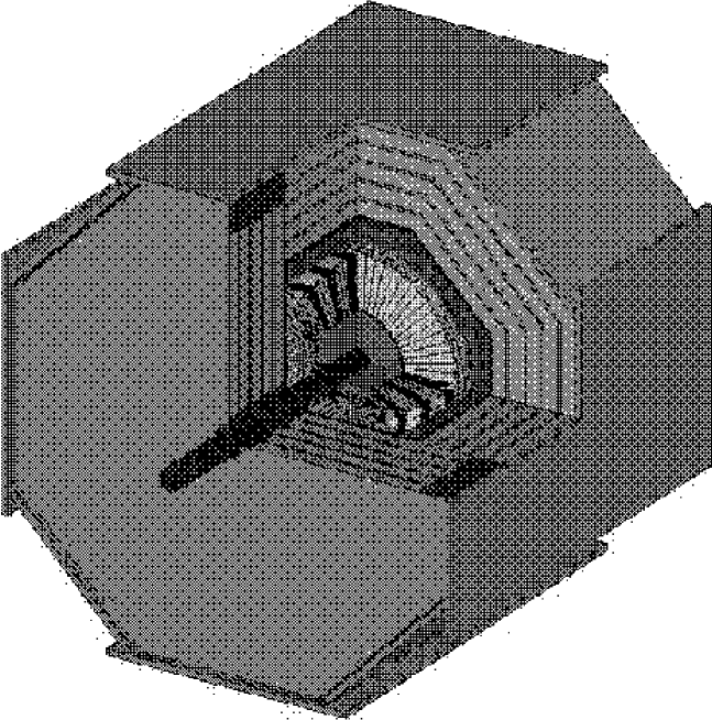
Figure 1.1: Configuration of the baseline JLC detector.

There has been a great progress in evaluating backgrounds to the tracking detectors these years. As a result, the magnetic field of 2 Tesla in the original design is now thought to be a little too weak to suppress backgrounds to the vertex detector (VTX) and the central drift chamber (CDC) in the case of high-luminosity operation (parameter set Y) of $2.5\times 10^{34}$cm²sec^-1. We therefore started studies for a new detector design with 3 Tesla magnetic-field, and consequently with smaller dimensions. This is why, for some sub-detectors described in the detector chapters, both the 2 Tesla- and the 3 Tesla-designs are discussed in parallel. Inner detectors, on the other hand, have common designs, regardless of the field choice, as far as the aforementioned two options are concerned.

As a matter of fact, there has been a proposal to go to much higher magnetic field and much smaller size. However, studies on this compact-detector option are yet very limited, and thus are omitted in this report.

In designing the 3 Tesla-version, some detector parameters have been revised in accordance with progress in each sub-detector R&D and of simulation studies. There has also been significant advance in detector technologies as consequences of SSC, Tevatron, and LHC studies. Some sub-detector designs have been revised to utilize these new technologies.

Fig. 1.1 shows a cut view of the present (revised) JLC detector of the 3 Tesla design. From inside to outside in the radial direction, it is composed of VTX, an Intermediate Silicon Tracker (IT), the CDC, a Calorimeter (CAL), a Superconducting Solenoid, and Muon Counters (MU) interleaved with flux-return iron yokes. There is a supporting tube between the IT and the CDC, which supports inner detectors and Interaction Region (IR) devices such as VTX, the IT, Luminosity and Pair Monitors (LM and PM), final Q-magnets, conical masks with active energy taggers (AM) on their tips, and compensating solenoids. There is no design for forward trackers (FT) yet. The overall dimension of the 3 Tesla design is about $14{\rm m}\times 14{\rm m}\times 13{\rm m}$, and weighs about 13 kilo-tons. This volume is slightly smaller than that of the CMS detector at LHC.

Key parameters and expected performances of the sub-detectors are summarized in Table 1.1. Notation of sub-detectors in the table follows the abbreviations given above.

Table 1.1: Parameters and Performances of the baseline JLC detector.

Key points of the sub-detector R&D’s are very briefly listed below.

IR

The most important tasks of the IR study are:

• to design beam line devices which minimize backgrounds to the detectors,

• to estimate the backgrounds to the detectors reliably,

• to design a radiation-resistant detector for the pair monitor, and

• to design a stable support system for the IR devices.

Though there remains some technical issue to be solved, most of these tasks are satisfactorily achieved as described in Chapter 7.

Trackers

The most crucial R&D item on the VTX detector is radiation hardness of CCD. The most up-to-date technologies such as two-phase operation and notch structure seem promising to enable operation of a few years to several years. However, further establishment is needed. Other R&D items such as position resolution, room-temperature operation, and fast readout are shown to be of no problem. Detail will be presented in Chapter 8.

Many R&D items of the CDC are related to the feasibility of a 4.6m-long chamber: wire creep, wire sag, stereo-cell geometry, or a thin mechanical structure which can support huge wire tension. These problems may disappear in the case of the 3 Tesla design. However, the 3 Tesla-field raised a new problem: large Lorentz angle. Some of the problems above are almost solved, while others need further studies.

Generic studies such as gas gain, position resolution, and two-track separation, on the other hand, are straightforward tasks, and seem to be almost established. These items will be described in Section 8.3.

Studies on the IT are yet rather limited. Simulation studies on its performance are in progress with a 1st trial set of parameters. Hardware design studies, however, are very primitive. The description of the IT given in Section 8.2 is, therefore, mostly on the simulation results.

Studies on the forward trackers have not yet started.

PID

Studies are rather limited up to now about dedicated detectors for particle identification, especially for $\pi/K$ separation. Though it was reported that $dE/dx$ measurement with pressurized gaseous tracking detectors can provide good $\pi/K$ separation for momentum region below 30 GeV [29], this momentum region may not be high enough to improve $W$-charge determination via jet-mode at the highest energy. Furthermore, in our current scope, the JLC-CDC will not be pressurized. In such cases, challenging detectors such as a focusing DIRC [30] would be helpful. However, since there have been almost no systematic studies about possible impact of such detectors on physics sensitivity, no dedicated chapter for particle identification is given in this report.

CAL

Calorimeter design has been changed significantly since the JLC-I study report. Finer granularity is aimed at while keeping the best energy resolution. The latter has been established by series of test beam measurements, while optimization of granularity is still underway. Studies on photo-detectors and engineering issues are also in progress. The detail of the study including historical review is presented in Chapter 9.

MU

Requirements on muon detectors are neither so severe nor unique under linear collider environment. We therefore think that muon detectors developed for B-factories or for LHC experiments will be usable for linear collider experiments. Applicability of such muon detectors is examined in Chapter 10.

DAQ

The number of read-out channels and average data size are listed in Table 1.1. Zero-suppression-on-board is assumed for the data-size estimation.

The CCD-VTX detector was once thought to be too slow to finish readout within the bunch-train crossing-interval of 6 msec, and various pre-processing schemes were investigated. Recent studies have shown that it is feasible to read-out all the CCD data during the train-crossing interval. Therefore all the data from all the sub-detectors can directly be transfered to a CPU farm for judgement. Since there is no complicated architecture in the DAQ design, dedicated chapter is not given in this report.

Structure

In Chapter 11, design of the solenoid structure and its engineering studies on mechanical and magnetic properties are described. Because of the huge magnetic force on the endcaps we may end up with reducing the number of super-layers of the muon detector interleaved with the endcap iron yokes in the case of the 3 Tesla design. Otherwise there is no foreseen difficulty, and one possible solution, though not yet final, is presented.

Simulation Tools

Two kinds of detector simulators, QuickSim and JIM, have been used for our studies. QuickSim is a simple but fast simulator mostly used for physics studies. JIM is a full detector simulator based on the Geant3 packages and used for studies of detector performance. These tools are described in Chapter 12, together with tools for event generations. Recently, we started developing a new full detector simulator, JUPITER, using object oriented technology based on Geant4. Short report on its status is also given there.

1.4 Accelerator Overview

1.4.1 Accelerator Complex

A detailed report on the R&D status as of 1997 was published as ‘JLC Design Study’[31] and recent updates are described in ‘ISG Progress Report’[32]. Look at the web pages[33] for the latest status. Here, we shall summarize the machine aspects very briefly.

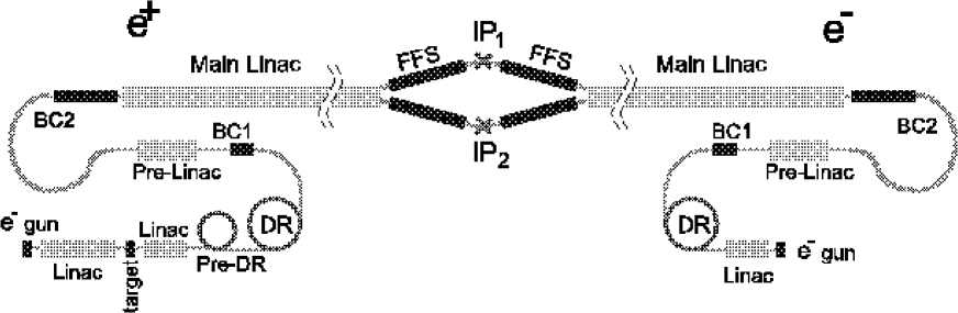
Figure 1.2: Schematic Layout of JLC. Not to scale. DR: Damping Ring, BC: Bunch Compressor, FFS: Final Focus System, IP: Interaction Point.

The whole accelerator complex is schematically depicted in Figure 1.2.

Injectors

The e⁺e^- beams to be injected to the main linacs have the following properties:

• The beam energy 10 GeV.

• One pulse consists of 95 bunches with the separation 2.8 nsec in-between (190 bunches $\times$ 1.4 nsec when upgraded).

• Each bunch contains $\sim 10^{10}$ particles. The r.m.s. bunch length is $\sim 100~{}\mu$m.

• The pulse is repeated at 150 Hz.

The electron beam is created in the following scenario:

• The beam generated by the electron gun is accelerated to 1.98 GeV by an S-band linac and cooled to the required emittance in the damping ring (DR).

• The bunch length is $\sim$5 mm when extracted from DR. It is compressed by the first bunch compressor BC1 to $\sim 500~{}\mu$m.

• Accelerated to 10 GeV by another S-band linac (pre-linac).

• The bunch is compressed to the desired length in the second bunch compressor BC2. BC2 is a fairly large structure, consisting of a large arc ($\sim$300 m long), RF cavities ($\sim$300 m long), and a chicane. This makes a 180-degree turn so that the pre-linac and the main linac can be accommodated in the same tunnel.

For the positron beam some more facilities are needed:

• A high intensity electron beam is accelerated to $\sim$10 GeV and is led to a target to generate positrons.

• This positron beam is collected and accelerated to 1.98 GeV.

• Since the emittance is much larger than that of the electron beam from the gun, this positron beam is once cooled in the pre-damping ring before it is injected to DR.

Table 1.2: Main Linac RF System.

Overall parameters
Unloaded gradient	$G_{0}$	72	MV/m
RF System Efficiency	$\eta_{AC\rightarrow RF}$	38	%
Repetition rate	$f_{rep}$	100 or 150	Hz
Modulator
Efficiency	$\eta_{mod}$	75	%
Klystron
Klystron Peak Power		75	MW
Klystron Pulse Length		1.5	$\mu$s
Efficiency	$\eta_{kly}$	60	%
Pulse Compressor
Pulse compression method		2 mode 4/4 DLDS
Pulse compression power gain		3.4
Efficiency	$\eta_{compr}$	85	%
Accelerating Structure
Structure type		RDDS $2\pi/3$ mode
Structure length	$L_{s}$	1.80	m
Number of cells		206
Average iris radius	$\left\langle{a/\lambda}\right\rangle$	0.18
Attenuation parameter	$\tau$	0.47
Shunt impedance	$r_{s}$	90	M$\Omega$/m
Fill Time	$T_{f}$	103	ns
Q-factor	$Q$	7800

Main Linac

The acceleration scheme of the main linac is a conventional one: The electric power from commercial line is converted to a high-voltage (a few hundred kilo-volts), short (a few microseconds) pulse by klystron modulators. This pulse is converted into microwave by high-power klystrons and is led to normal-conducting accelerating structures. What is not conventional is that a very high accelerating gradient is required to make the whole system reasonably short. Generally speaking, a higher accelerating frequency of microwave is better for higher gradient but is more difficult technologically. There are at present two possible choices of the main accelerating frequency, X-band (11.424 GHz) and C-band (5.712 GHz), both being higher than conventional frequencies for linacs. The latter is considered to be a backup scheme in case the X-band R&D would delay or fail.

The development of high-power klystrons is going well but the technological limit of the klystron peak power is far below the value needed to reach the desired accelerating gradient (over 50 MV/m for X-band and over 30 MV/m for C-band). On the other hand it is relatively easy to obtain a long klystron pulse. Therefore, one should compress the pulse to obtain a higher peak power with shorter length. The pulse compression scheme is different between X- and C-band designs. The X-band design adopts the DLDS (Delay Line Distributed System) as the effective pulse compression method. The output microwaves (1.5 $\mu$sec long) from 8 klystrons are combined and cut into four in time. Each time slice is delivered to different accelerating structures upstream. The C-band design adopts a disk-loaded structure made of 3-cell coupled-cavity. The power efficiency is lower than the DLDS but the system is much more compact. In the following we shall describe the X-band design. The parameters related to the X-band RF system are summarized in Table 1.2.

1.4.2 Overview of JLC Parameters

The latest parameter sets are available in the ISG (International Study Group) Progress Report[32]. Here, we shall briefly summarize the major points and add some more detailed description on the issues related to the beam properties at the collision point.

Standard Parameter Sets

During the ISG study we have put emphasis on the cost and power minimization and the relaxation of the tolerances against various errors. As a result we decided not to give one single parameter set but to give a range of parameters in the form of three different sets A, B, and C. These do not mean three different designs but three different operation modes of the same machine. Basically, A adopts a low-current and small-emittance beam and C a high-current and large-emittance (i.e., accepts larger emittance growth). We demand that any of these operation modes (actually continuously from A to C) can be realized. For example the injector system should be able to deliver the highest current assigned for C and the bunch compressors can produce the shortest bunch for A.

Table 1.3 shows the parameter sets A, B, and C at the center-of-mass energy $W_{cm}\simeq 500$ GeV.

The luminosity values in Table 1.3 do not include the crossing angle at the collision point. To avoid background events we are thinking of a (full) crossing angle $\phi_{c}=7$ mrad, which will cause a luminosity reduction of about a factor 0.6. This reduction can be avoided by introducing the so-called crab crossing.

The SLC has provided a polarized electron beam ($\sim$80%). This will also be possible in JLC. The polarized electron gun for multi-bunch operation is not ready yet but is expected to be feasible by the time of JLC completion. The depolarization by the beam-beam interaction will be a few percent.

Upgrade of Luminosity

When the machine is well tuned after several years of operation, we may hope that the machine can be operated at a high current like C with a small emittance like A giving a very high luminosity. This parameter set is not consistent in that (1) the beamstrahlung would be too strong and (2) the alignment tolerance too tight. However, we can overcome these difficulties if we split the charge of each bunch into two bunches. We cannot change the total train length because of the pulse compression system already built. Thus, we have to halve the distance between bunches keeping the total train length. Thus, we come to the parameter set X shown in Table 1.3. The changes from A to X are to

• Increase the number of bunches from 95 to 190 and halve the bunch distance to 1.4 nsec. (To do so an absolute constraint in the design stage is that the RF frequencies lower than 714 MHz must not be used.)

• Set the bunch charge to 0.55$\times 10^{10}$ so that the total charge in a train is the same as in C.

• Improve the vertical emittance from the damping ring by a factor 2/3 and keep the same emittance blowup ratio in the main linac as in A (absolute blowup is smaller).

• Slightly shorten the bunch length.

• Slightly improve the beta functions at the IP, which is expected to be feasible at energies much lower than the highest design energy (1 to 1.5 TeV).

The beamstrahlung and alignment tolerance of accelerating structures are better than in the standard sets owing to the greatly reduced bunch charge. Thus, a further upgrade of luminosity will be possible if we can increase the bunch charge back to that in A, resulting in the parameter set Y. (Note that the linac must slightly be lengthened to achieve Y due to the lower loaded gradient.) However, this parameter set demands very high beamloading everywhere in the system. Also, a higher production rate of positrons (factor 1.27 over C) is required.

Table 1.3: Parameters for the JLC at $E_{CM}\simeq$500 GeV

		A	B	C	X	Y
Beam parameters
Center-of-mass energy	$E_{CM}$	535	515	500	497	501	GeV
Repetition rate	$f_{rep}$	150					Hz
Number of particles per bunch	$N$	0.75	0.95	1.10	0.55	0.70	$10^{10}$
Number of bunches/RF Pulse	$n_{b}$	95			190
Bunch separation	$t_{b}$	2.8			1.4		ns
R.m.s. bunch length	$\sigma_{z}$	90	120	145	80	80	$\mu$m
Normalized emittance at DR exit	$\gamma\varepsilon_{x}$	300			300		$10^{-8}$m$\cdot$rad
	$\gamma\varepsilon_{y}$	3.0			2.0		$10^{-8}$m$\cdot$rad
Main Linac
Effective Gradient1)	$G_{eff}$	59.7	56.7	54.5	54.2	50.2	MV/m
Power/Beam	$P_{B}$	4.58	5.58	6.28	6.24	7.99	MW
Average rf phase	$\phi_{rf}$	10.6	11.7	13.0			deg.
Linac Tolerances	$y_{c}$	16.1	15.2	14.6	18.	14.	$\mu$m
Number of DLDS nonets		23				25
Number of structures per linac		2484				2700
Number of klystrons per linac		1656				1800
Active linac length		4.47				4.86	km
Linac length		5.06				5.50	km
Total AC power	$P_{AC}$	118				128	km
IP Parameters
Normalized emittance at IP	$\gamma\varepsilon_{x}$	400	450	500	400	400	$10^{-8}$m$\cdot$rad
	$\gamma\varepsilon_{y}$	6.0	10	14	4.0	4.0	$10^{-8}$m$\cdot$rad
Beta function at IP	$\beta_{x}$	10	12	13	7	7	mm
	$\beta_{y}$	0.10	0.12	0.20	0.08	0.08	mm
R.m.s. beam size at IP	$\sigma_{x}$	277	330	365	239	239	nm
	$\sigma_{y}$	3.39	4.88	7.57	2.57	2.55	nm
Disruption parameter	$D_{x}$	0.0940	0.117	0.136	0.0876	0.112
	$D_{y}$	7.67	7.86	6.53	8.20	10.43
Beamstrahlung param	$\left\langle{\Upsilon}\right\rangle$	0.14	0.11	0.09	0.127	0.163
Beamstrahlung energy loss	$\delta_{B}$	4.42	4.09	3.82	3.49	5.22	%
Number of photons per $e^{-}/e^{+}$	$n_{\gamma}$	1.10	1.20	1.26	0.941	1.19
Nominal luminosity	${\cal L}_{00}$	6.82	6.41	4.98	11.15	18.20	$10^{33}\mbox{cm}^{-2}\mbox{s}^{-1}$
Pinch Enhancement2)	$H_{D}$	1.444	1.392	1.562	1.389	1.483
Luminosity w/ IP dilutions	${\cal L}$	9.84	8.92	7.77	15.48	27.0	$10^{33}\mbox{cm}^{-2}\mbox{s}^{-1}$

1) Effective gradient includes rf overhead (8%) and average rf phase $\left\langle{\cos\phi_{rf}}\right\rangle$.
2) $H_{D}$ includes geometric reduction (hour-glass) and dynamic enhancement. The focal points of the two beams are made separated to each other by about $1\sigma_{z}$ for higher $H_{D}$ ($\sim$10%)

Scaling to Lower Energies

For given normalized emittance $\gamma\epsilon_{x}$ and $\gamma\epsilon_{y}$, the beam size at the IP scales as $1/\sqrt{W_{cm}}$ so that the luminosity is simply proportional to $W_{cm}$. This is not correct, however, if one lowers the energy by reducing the accelerating gradient. The beam loading effect is characterized by the ratio of the beam-induced field to the external field (by klystron). Therefore, when one reduces the accelerating gradient, one has to reduce the charge proportionally for avoiding too large beam loading. Thus, the luminosity would scale as $W_{cm}^{3}$, which is not acceptable for low energy experiments. For high luminosities we have to keep the gradient as high as possible. One might think that one can accelerate the beam to the desired energy and let the accelerated beam go through the empty accelerating cavities. This does not work because the beam-induced field in the empty cavities will destroy the beam quality. Thus, to get the luminosity scaling $\propto W_{cm}$, one has either

• to perform low energy experiments during the construction stage when the unnecessary accelerating structures have not yet been installed

• or to construct a bypass system such that the beam accelerated to a desired energy skips the rest of the linac and is directly transported to the final focus system. (See Figure 1.3)

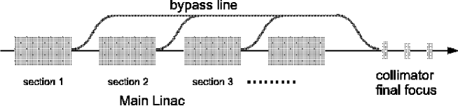
Figure 1.3: Schematic layout of the bypass

Obviously neither of these can be continuous: the construction stage is discrete and the bypass line as well. Thus, large changes of energy should be made by the above ways and fine adjustment by changing the gradient. Table 1.4 shows the scaling of parameters (for each of A,B,C,X,Y) under the two conditions: (a) constant gradient and (b) constant active linac length. For example, if one wants $W_{cm}$=250 GeV but only a bypass for 300 GeV is available, the luminosity will be $(300/500)\times(250/300)^{3}$ times the luminosity at 500 GeV. We do not have a design of the bypass system yet.

Table 1.4: Energy scaling of parameters for (a) constant gradient and (b) constant active linac length. The numbers are the power of $W_{cm}$. The luminosity($\dagger$) is not rigorous due to the change of pinch enhancement factor. Beamstrahlung energy loss and the number of beamstrahlung photons($\ddagger$) are not rigorous due to the change of $\Upsilon$.

	(a)	(b)
Luminosity ${\cal L}$ ${}^{(}\dagger)$	1	3
Bunch charge $N$	0	1
Bunch length $\sigma_{z}$	0	0
IP beam size $\sigma_{x}$, $\sigma_{y}$	-0.5	-0.5
Disruption parameters $D_{x}$, $D_{y}$	0	1
Upsilon parameter $\Upsilon$	1.5	2.5
Beamstrahlung energy loss (relative) ${}^{(}\ddagger)$	2	4
Number of beamstrahlung photons ${}^{(}\ddagger)$	0.5	1.5

Beam Energy Spread

The beam energy spread before collision is normally a small fraction of a percent and is much smaller than the effect of the beamstrahlung. Nonetheless, the beam energy spread can be important, depending on the type of experiments, because the high-energy spectrum edge still remains under the beamstrahlung but will be blurred by the energy spread of the input beam.

The beam energy spread within a bunch comes from

• effect of the short-range longitudinal wake (beam-induced field within a bunch)

• energy spread before the main linac

The latter is small ($\leq 2\mbox{\%}\times\mbox{10~{}GeV}/E$) except for experiments at very low energies. We can minimize the former, which causes more energy loss at the bunch tail than at the head, by placing the bunch at the optimum phase of the sinusoidal curve of the accelerating field. The phase angle is also used for other purpose (to control the transverse instability) but a control of the energy spread can still be possible by changing the phase in upstream and downstream parts of the linac separately, since the instability is severer in the low energy part. In general, an under-correction (small phase) causes a doubly-peaked distribution with a short tail and an overcorrection causes a sharp single peak with a long tail.

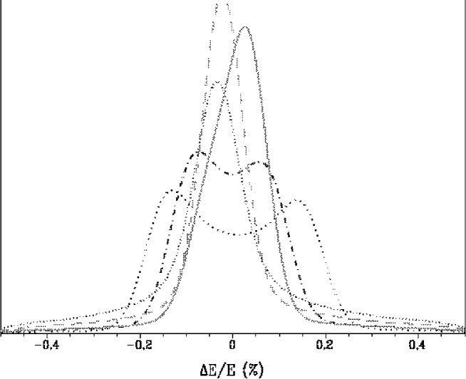
Figure 1.4: An example of beam energy spread at 250 GeV changing the RF phase. An initial spread of 1.5% (rms) at 10 GeV has been added.

Figure 1.4 shows an example of the energy spectrum at various RF phases for the parameter set A at the beam energy 250 GeV. The vertical scale is normalized for each curve. An initial energy spread of 1.5% (rms) at 10 GeV has been added in this figure.

In addition to the above spread within a bunch, there will be a fluctuation of average energy from bunch to bunch and from pulse to pulse. The possible reasons are:

• miss-compensation of beam loading

• jitter of the klystron power and phase

• change of beam loading due to the fluctuation of the pulse charge

• jitter of the longitudinal bunch position when the bunch enters the linac.

We shall try to keep them within $\pm$0.1%. The measurement of the average beam energy over each pulse will be possible at the linac exit with an accuracy better than 0.1%. It will also be possible to measure the energy of each bunch by using improved fast position monitors. Then the effects of the energy fluctuation listed above (but not the spread like the wake effect) can effectively be eliminated in the software level (i.e., the collision energy of each bunch is known although it fluctuates).

An energy feedback is possible if the fluctuation is slow enough (lower than $\sim$10 Hz) but the energy spread within a bunch cannot be corrected.

Luminosity Spectrum

The electrons(positrons) emit synchrotron radiation during the collision due to the electromagnetic field (several kilo Tesla) created by the opposing beam. This phenomenon is called ‘beamstrahlung’. Due to the beamstrahlung the particles loose a few percent of their energies on the average. This causes a spread in the center-of-mass energy in addition to the initial beam energy spread from linacs.

The expected luminosity spectrum $d{\cal L}/dW_{cm}$ is plotted in Figure 1.5 for A and Y. The high-energy end is shown in Figure 1.6. For these figures $W_{cm}$ is adjusted to 500 GeV for the convenience of comparison so that the luminosities are slightly different from those in Table 1.3. (Linear $W_{cm}$ scaling rather than $W_{cm}^{3}$ is used here.) The beam energy spread before collision is not included. In Figure 1.6 the highest bin ($499.75\leq W_{cm}\leq 500$ GeV) contains 49% (46%) for A (Y) of the total luminosity.

Both the luminosity and the average loss by beamstrahlung is proportional to the bunch population squared. When the parameter set A is achieved and if a much narrower energy spread is desired, one can reduce the beamstrahlung loss by a factor of four by making the bunch population half but with pulse structure the same as in Y. The reduction of luminosity from A is only a factor of two rather than four. This is technically even easier than A (same loading, relaxed tolerances).

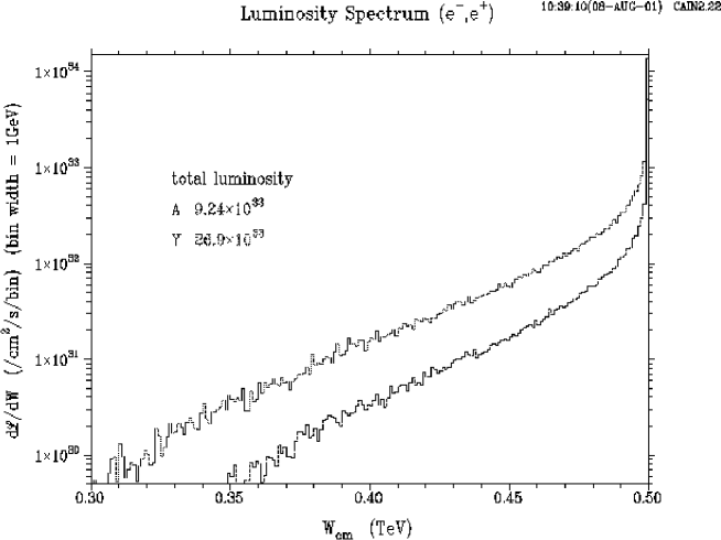
Figure 1.5: Luminosity spectrum at $W_{cm}$=500 GeV for the parameter set A (thin solid) and Y (solid). The beam energy spread before collision is not included.

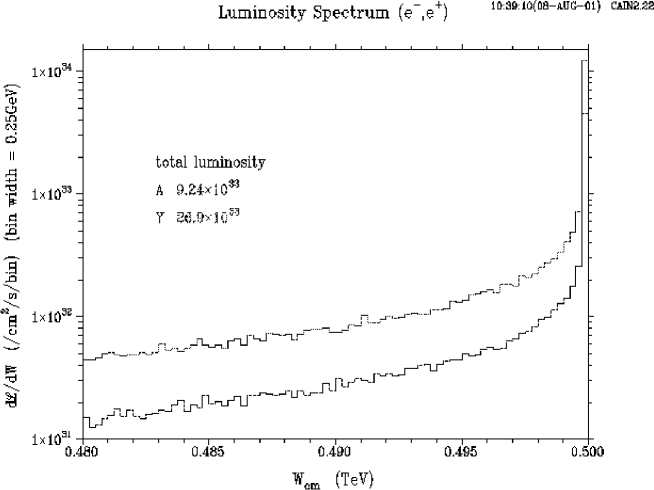
Figure 1.6: High-energy end of the luminosity spectrum at $W_{cm}$=500 GeV for the parameter set A (thin solid) and Y (solid). The beam energy spread before collision is not included.

Part II Physics

Chapter 2 Higgs

2.1 Introduction

We report Higgs physics at JLC based on the recent progress in the experimental and theoretical studies. We focus on the discoveries and measurements expected to be achieved at the first phase of the JLC project $\sqrt{s}=$250–500 GeV, especially at the early stage of low energies at $\sqrt{s}\approx 300$ GeV. The key measurements and the problems to be solved before the experiment are discussed. We first start from the astonishing Higgs discovery sensitivity at JLC, followed by discussions how to define the quantum number for the found new particle in order to confirm it is indeed Higgs particle. Next step is to measure the Gauge coupling. The measurements of Yukawa couplings with leptons and quark flavours including top are one of the highlights of the Higgs study. The experimental studies are based on detector performance expected in the JLC-I detector. Based on the results obtained so far in the simulation studies, impacts on the physics and models are discussed from theoretical view points. The studies of the Higgs boson [1] is the key to open the future generation of the particle physics. Our understanding of nature based on the local gauge principle demands a scheme to make gauge boson and quark/leptons massive. The origin of the mass is either fundamental scaler particle, Higgs boson, or new interaction such as technicolor.

The existence of the Higgs boson is of course the first question to be answered by experiments. If it is found to exist, the next essential questions are how many Higgs bosons, and how the relations are between couplings and masses of quark/lepton/gauge-bosons. The Standard Model (SM) [2] assumes a single Higgs field doublet, hence the single physical state $\mathrm{H}^{0}$ generates masses of quark/lepton and Z/W with completely defined couplings except for the Higgs boson mass itself. There are also varieties of models in extensions of the SM in the Higgs sectors, and nobody knows the answer to the questions.

As one knows the SM Higgs sector has various problematic issues inside such as the fine-tuning problem. The Higgs couplings and their evolutions are significantly sensitive to the fundamental structure of interaction and contents of particles up to GUT scale ($\sim 10^{16}$ GeV) via loop effects, which becomes one of the strong motivations to introduce the supersymmetry (SUSY). Even in the Standard Model, the mass of the Higgs has both upper and lower values by vacuum stability and self-coupling evolution depending on the cutoff scale. Hence the Higgs study is a strong tool to look into physics up to GUT scale.

Currently running B-factories in Japan and US measure the CKM matrix parameters in order to investigate the origin of CP violation. Also neutrino physics studied at SuperKamiokande together with K2K project in Japan look into the mass and mixing in the lepton sector. The mass matrix in quark and lepton sectors is an obvious key, hence the origin of the mass of the fundamental particles investigated at JLC, together with the results to be obtained at B-factory and SuperKamiokande/K2K, would give us a comprehensive views for the origin of the flavour mixing, CP violation, and a road to understand why 3 generations exist in our Nature.

Possible scenario for the first discovery depends on the Higgs in models. At LEP in 2000, an indication of possible signal has already obtained at a mass of 115 GeV [3]. If this signature indeed comes from a Higgs boson, it would be confirmed at Tevatron [4] and/or LHC [5] in years around 2007 since it is the SM-like Higgs boson. So far the lower mass bound of the SM Higgs is around 113 GeV and about 90 GeV for the Higgs in the minimal supersymmetric extension of the SM (MSSM) [6] (h⁰, A⁰) at the 95 % CL from LEP-II [3, 7]. Tevatron run2 in the following years is expected to be sensitive to discover the SM Higgs of its mass up to 120 GeV or more [4] provided the integrated luminosity exceeds a few fb^-1. At forthcoming LHC, there are varieties of channels in the SM and MSSM in which we have large discovery potential with significance 5–10$\sigma$ in wide range of the mass of the Higgs bosons [5], while the detectable channels are limited due to huge backgrounds in the $pp$ collisions and also the production yield and detection efficiency could be much lower if nature is further beyond the MSSM. Note that the experimental boundary in the extension of the SM in general two Higgs field doublet models (2HDM) is much weaker [9] than that of the SM or MSSM Higgs. For the charged Higgs boson predicted in the 2HDM has been looked for only up to around 80 GeV [7].

The Higgs discovery itself is significantly easier at LC than Tevatron/LHC, provided that we establish JLC with luminosity of order of 10³⁴ cm^-2s^-1 at the beam energy high enough to produce Higgs boson kinematically, $\sqrt{s}>\mbox{$m_{\mathrm{Z}}$}+\mbox{$m_{\mathrm{H}}$}$. We need only “one day” running to discover the SM-like Higgs, which is extremely different situation from other experiments like LHC. Even for the SUSY models beyond the MSSM, there always exist the lower limits of the production cross-section for at least one CP-even Higgs. Extremely less and well defined background at JLC compared to hadron colliders enables us to discover Higgs boson, even if the cross-section is 10 times smaller than the lower limits predicted by SUSY models.

The possible mass regions of the lightest Higgs boson differ model by model. There are, however, strong indications that the mass is lower than 250 GeV where the first phase of JLC project covers well without questions. The indirect measurements of the electroweak parameters at LEP/SLC/Tevatron with recent measurements of hadronic cross-section at BEPC [10] in China give an upper mass bound of about 215 GeV at the 95% CL [8] for the SM Higgs. When we assume the MSSM, the mass must be lower than 140 GeV. With an additional SU(2) singlet to the MSSM (NMSSM), the upper bound is about 140 GeV assuming the finite Higgs coupling up to GUT scale [11], and even in more general scheme in SUSY the bound does not exceed 210 GeV [12]. Hence the observation of at least one Higgs is guaranteed unless our understanding of the nature is completely wrong. One can say, in other words, it is really a “big discovery” when we find no Higgs at JLC phase-I.

At the first phase of JLC, apparently the target Higgs mass is from 100 GeV (just above the current LEP boundary) to 250 GeV. Our purpose of the experiment at JLC is not only to judge the existence of the light Higgs predicted in the SM or SUSY, while we may have an opportunity to reject some of above models of Higgs sectors only from the observed mass of the Higgs as are discussed above.

The real Higgs physics starts after the discovery, in order to define the Lagrangian, and to scope the physics up to GUT scale. The important feature in JLC is its well defined background, and high purity of the signal. We expect to select more than 10⁵ Higgs events in 3–5 years running with background contamination less than 20%. The JLC gives us the unique opportunity to measure the cross-section and the branching ratio in percent order or even per-mill level in its error, which results in the precise measurements of the Higgs gauge coupling, Yukawa-coupling, and furthermore derivation of Higgs self-couplings in multi-Higgs production. All of these measurements can be made in model independent fashion. And then, relations among the couplings predicted in models can be cross-checked in various measurements. The scenario of the CP-even Higgs hunting/measurements at JLC is as follows; the first we start from model independent measurements:

1. If Tevatron or LHC missed it, JLC discovers Higgs.

2. Mass measurement.

3. Cross-section measurement.

4. CP, spin determination by the angular distributions, energy scan with/without polarized beam option.

5. Establishment of ZZH coupling.

6. Gauge coupling (F_ZZH, F_WWH) measurements.

7. Yukawa coupling ($\lambda_{\tau}$, $\lambda_{b}$, $\lambda_{c}$, $\lambda_{t}$) measurements.

8. Natural width ($\Gamma_{H}$) measurement.

9. Self-coupling ($\lambda$) measurement.

Even after the discovery of a Higgs particle, many unexpected discovery which means further beyond SM/SUSY might yet wait for us at JLC. In the SM and SUSY models, there always have numbers of relations in couplings. We ask; if coupling to Z and W relates as expected from SU(2)$\times$U(1) symmetry breaking?; if ratio of Yukawa coupling for tau and b is really the ratio of these masses?; if all 3 generations of up (down) type quarks have the same coupling normalized with mass?; and if CP is conserved in Higgs sector?

These precisely measured values are also used to severely check the SM, SUSY models and others. In the SM, the couplings are completely determined by the measured SM parameters. Once we put the mass of the Higgs, all are calculable. Thanks to the complete initial state of ${\mathrm{e}}^{+}{\mathrm{e}}^{-}$ collision at JLC, the cross-section for the SM is theoretically known within less than 1% accuracy. Yukawa coupling for tau has been constrained within per-mill. Yukawa coupling for b-decay is known within a few %, and the accuracy will increase furthermore by data from the B-factories. If one measures the couplings within percent level, we can severely check the SM at the level of the virtual effect from other Higgs or SUSY particles. We also translate the precisely measured model-independent values to other model parameters such as tan$\beta$ or $\alpha$ for MSSM as an example. We check the internal consistency (universality) in the translated parameters from various measurements. If we have other Higgs mass lighter than TeV, we would have such effects at percent level or more. In other words we can measure the mass of the other Higgs depending on the models. At next phase of JLC, LHC or even already in JLC phase-I, we look into the predicted mass, and can determine the final Lagrangian of the Higgs sector. The couplings and other physics parameters are finally examined in the models of the Grand Unification using renormalization group evolution. Precise measurements of Higgs properties at JLC are essential tool to give definite answers to physics models and to determine the fundamental structure of the interaction in nature up to GUT scale.

This report discuss the recent Higgs studies at JLC which have been made in ACFA Higgs working group [13, 14] and as a regional studies for the world-wide LC Higgs cooperation [15]. The studies in experimental feasibility does depend significantly on the accelerator and detector performance. Hence in this report as a first priority we made following direction:

• Studies based on recent JLC-I [17] detector design (see Part III) as a model detector, using the fast [18] and full [19] detector simulation softwares (see Chapter 12).

• Recent accelerator parameters, such as beamstrahlung [21, 20].

• Concentrate on the JLC phase-I energy (250–500 GeV), especially for the energy at early stage ($\sqrt{s}\leq 350$ GeV).

• Studies on light Higgs ($\mbox{$m_{\mathrm{H}}$}<210$ GeV) predicted in the SM and SUSY models, especially for 120–140 GeV region where the variety of decay branch can be simultaneously studied.

• Emphasize on the measurements independent to models, since nobody knows the true model.

• Simulation tests in the realistic experimental environment [22].

The important but missing ingredients in this report for the Higgs studies at JLC program such as multi-Higgs production, Heavy Higgs, measurements of coupling with SUSY particles, precise measurement of top-Yukawa coupling, self-coupling and its running measurements, are only simply described. The direction and feasibility of these studies depends on the physics results at the initial stage of the JLC phase-I. The energy and luminosity should be optimized for these studies; either quick upgrade of the energy, or concentrate on the lower energy and accumulate the integrated luminosity furthermore. The studies are open for the next ACFA report.

2.2 Theoretical Overview

In the minimal SM, we introduce only one Higgs doublet field. The Higgs potential is given by

$$V=-\mu^{2}|H|^{2}+\lambda|H|^{4}.$$ (2.1)

Through the electroweak symmetry breaking, the gauge bosons, fermions and the Higgs boson receive their masses. At the tree level, the mass formulae are given by $m_{W}=\frac{1}{2}gv$ for the $W$ boson, $m_{Z}=\frac{1}{2}\sqrt{g+g^{\prime}}v$ for the $Z$ boson, $m_{f}=\frac{y_{f}}{\sqrt{2}}v$ for fermions and $m_{H}=\sqrt{\lambda}v$, where $v(\simeq$ 246 GeV) is the Higgs vacuum expectation value, $g$ and $g^{\prime}$ are SU(2) and U(1) gauge coupling constants, and $y_{f}$ is the Yukawa coupling constant for the fermion $f$. These expressions imply that a particle mass is determined by the strength of its interaction to the Higgs field, therefore the measurement of the coupling constants related to the Higgs boson is an important check of the mass generation mechanism in the SM.

In particular, the formula $m_{H}=\sqrt{\lambda}v$ suggests that the mass of the Higgs boson reflects the strength of the electroweak symmetry breaking dynamics. The heavy Higgs boson implies the strongly-interacting dynamics and the light Higgs boson is consistent to the weakly interacting scenario such as grand unified theory (GUT) or supersymmetric (SUSY) unified models. Although the Higgs boson mass is a free parameter within the minimal SM, we can determine the upper and lower bound of its mass, if we require that the SM is valid up to some cut-off scale, beyond which the SM should be replaced by a more fundamental theory. If the cut-off scale is taken to be the Planck scale $(\sim 10^{19})$ GeV, the possible mass range is 135 - 180 GeV. For a larger mass the Higgs self-coupling constant blows up below the Planck scale, and for a lower mass the vacuum stability is not guaranteed.

There are many possibilities to extend the Higgs sector of the minimal SM. Because the $\rho$ parameter determined from the electroweak measurements is close to unity, the dominant contribution to the electroweak breaking should come from weak-doublet fields. Two Higgs doublet model is one of the simplest extensions. In this case, there are two CP-even Higgs bosons $(h,H)$, a CP-odd Higgs boson $(A)$ and a pair of charged Higgs bosons $(H^{\pm}$). If we require the two Higgs doublet model is valid up to the cut-off scale, the mass range of the lighter CP-even Higgs boson $(h)$ is determined in a similar way to the SM case. For the case that the Planck scale is the cut-off scale, the upper-bound is 180 GeV, just like the SM. The lower bound can be smaller than the corresponding mass bound in the SM. In particular, the lower-bound is about 100 GeV in the case that the only one SM-like Higgs boson becomes light compared to other Higgs states.

Since the present electroweak measurements are precise enough to be sensitive to virtual loop effects, we can put a useful bound on the Higgs boson mass, independent of the theoretical assumption on the validity of the theory up to some high energy scale. Within the minimal SM, the 95 % upper bound on the Higgs boson mass is about 210 GeV[8] using the direct measurements of the $W$ boson and top quark mass in addition to various electroweak data at LEP and SLD experiments. For more general model, for example in the two Higgs doublet model, this kind of strong bound is not obtained only from the electroweak data.

Since the end of 1970’s, it has been known that supersymmetry (SUSY) can be a solution of the naturalness problem in the SM. If we consider the cut-off scale of the SM is the Planck or the GUT scale, we need extremely precise fine-tuning in the renormalization of the Higgs mass term to keep the weak scale much smaller than the cut-off scale. There is no such problem in SUSY models because the problematic quadratic divergence in the scalar mass renormalization is absent. Motivated by this observation, SUSY extensions of the SM and the GUT were proposed, and many phenomenological studies have been done. For the last ten years, SUSY models has become the most promising candidate of physics beyond the SM, because the gauge coupling constants determined at LEP and SLD experiments turned out to be consistent with the prediction of the SUSY GUT scenario.

The simplest SUSY extension of the SM is called the minimal supersymmetric standard model (MSSM). The Higgs sector of the MSSM is the type-II two Higgs doublet model, where Higgs doublet fields $H_{1}$ and $H_{2}$ are introduced for the down-type quark/lepton Yukawa coupling and the up-type quark Yukawa coupling, respectively. We define two angle variables to parameterize the Higgs sector. One is the vacuum mixing angle given by $\tan{\beta}\equiv<H_{2}^{0}>/<H_{1}^{0}>$. The other is the mixing angel between two CP-even Higgs bosons $h$ and $H$, $(m_{h}<m_{H})$.

$$ReH_{1}^{0} = (v\cos{\beta}-h\sin{\alpha}+H\cos{\alpha})/\sqrt{2},$$ (2.2)

$$ReH_{2}^{0} = (v\sin{\beta}+h\cos{\alpha}+H\sin{\alpha})/\sqrt{2},$$ (2.3)

where $H_{1}^{0}$ and $H_{2}^{0}$ are the neutral components of two Higgs doublet fields. The ratio of various tree level coupling constants in the MSSM and those in the SM are listed in table 2.1.

Table 2.1: The coupling constant in the MSSM normalized by the corresponding coupling constant in the SM. In the Yukawa coupling for the CP-odd Higgs boson $(A)$, the fermion current is of the pseudo-scalar type.

$hWW,hZZ$	$HWW,HZZ$	$ht\bar{t}$	$hb\bar{b},h\tau\bar{\tau}$	$Ht\bar{t}$	$Hb\bar{b},H\tau\bar{\tau}$	$At\bar{t}$	$Ab\bar{b},A\tau\bar{\tau}$
$\sin{(\beta-\alpha)}$	$\cos{(\beta-\alpha)}$	$\frac{\cos{\alpha}}{\sin{\beta}}$	$-\frac{\sin{\alpha}}{\cos{\beta}}$	$\frac{\sin{\alpha}}{\sin{\beta}}$	$\frac{\cos{\alpha}}{\cos{\beta}}$	$\cot{\beta}$	$\tan{\beta}$

In the MSSM, we can derive the upper-bound of the the lightest CP-even Higgs boson mass $(m_{h})$ without reference to the cut-off scale of the theory. This is because the self-coupling of the Higgs field is completely determined by the gauge coupling constants at the tree level. Although $h$ has to be lighter than Z⁰ boson at the tree level, contribution from the loop effects by the top quark and stop squark can extend the possible mass region [23]. Taking into account the top and stop one-loop corrections, $m_{h}$ is given by

$$m_{h}^{2}\leq m_{Z}^{2}\cos^{2}{2\beta}+\frac{3}{2\pi^{2}}\frac{m_{t}^{4}}{v^{2}}ln{\frac{m_{stop}^{2}}{{m_{t}}^{2}}},$$ (2.4)

where we assume that two stop mass states have the same mass. More precise formula is available in the literature. It is concluded that $m_{h}$ is bounded by about 130 GeV, even if we take the stop mass to be a few TeV. The upper-bound of $m_{h}$ is shown in Fig 2.1.

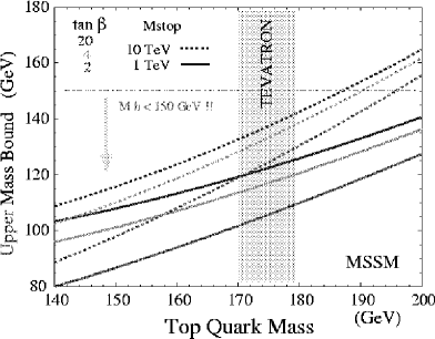
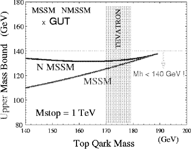
Figure 2.1: The upper bounds of the mass of the lightest CP-even Higgs boson in MSSM and NMSSM calculated by Y. Okada et al [11]. (Left) Upper bounds as a function of the top quark mass in the MSSM, with various MSSM parameters as shown in the plot. (Right) Upper bound for MSSM and NMSSM with additional constraints of the finite Higgs coupling up to GUT scale. The top quark mass measured at Tevatron is indicated by the grey bands.

The radiative correction can also change the mass formulas of the heaver Higgs bosons. The Higgs potential is parametrized by three mass parameters, gauge coupling constants and the parameters of the top and stop sector through the one-loop correction. The independent parameters can be taken as $\tan{\beta}$, and one of Higgs boson masses, which is usually taken as the CP-odd Higgs boson mass $(m_{A})$ and the top and the stop masses. More precisely, the parameters appearing in the formula of the radiative correction are not just one stop mass, but two stop masses, trilinear coupling constant for stop sector $(A_{t})$, the higgsino mass parameter $\mu$, and sbottom masses, etc. (If we use more precise formula, we need to specify more input parameters.) Once these parameters are specified, we can calculate the mass and the mixing of the Higgs sector. The Higgs boson masses are shown as a function of the CP-odd Higgs mass in Figure 2.2.

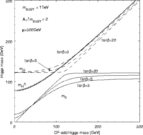
Figure 2.2: Higgs boson masses as a function of the CP-odd Higgs boson mass in MSSM.

It is important to distinguish two regions in this figure. Namely, when $m_{A}$ is much larger than 150 GeV, $H,A$ and $H^{\pm}$ states become approximately degenerate and the mass of $h$ approaches to its upper-bound value for each $\tan{\beta}$. This limit is called the decoupling limit. In this limit, $h$ has properties similar to the SM Higgs boson, and the coupling of the heavy Higgs bosons to two gauge-boson states is suppressed. On the other hand, if $m_{A}$ is less than 150 GeV, the lightest CP-even Higgs boson has sizable components of the SM Higgs field and the other doublet field.

Besides the Higgs potential, there is a case where radiative correction becomes potentially important for the MSSM Higgs boson phenomenology. For a large value of $\tan{\beta}$, SUSY correction can generate contributions to the bottom-higgs Yukawa coupling which is not present at the tree level[24]. The top and bottom Yukawa couplings with the neutral Higgs fields are given by

$$L_{Yukawa}=y_{t}\bar{t_{L}}t_{R}H_{2}^{0}+y_{b}\bar{b_{L}}b_{R}H_{1}^{0}+\epsilon_{b}y_{b}\bar{b_{L}}b_{R}H_{2}^{0*}+h.c.$$

The $\epsilon_{b}$ term is induced by loop diagrams with internal sbottom-gluino and stop-chargino. The bottom mass is then expressed by $m_{b}=y_{b}(1+\epsilon_{b}\tan{\beta})v\cos{\beta}/\sqrt{2}$. Although $\epsilon_{b}$ is typically $O(10^{-2})$, the correction to $m_{b}$ enters with a combination of $\epsilon_{b}\tan{\beta}$ which can be close to $O(1)$ for a large value of $\tan{\beta}$. Because of this correction, the ratio of $B(h\rightarrow\tau^{+}\tau^{-})$ and $B(h\rightarrow b\bar{b})$ is modified to

$$R_{\tau\tau/bb}\equiv\frac{B(h\rightarrow\tau^{+}\tau^{-})}{B(h\rightarrow b\bar{b})}=\left(\frac{1+\epsilon_{b}\tan{\beta}}{1-\epsilon_{b}/\tan{\alpha}}\right)^{2}R_{\tau\tau/bb}(SM),$$ (2.5)

where $R_{\tau\tau/bb}(SM)$ is the same ratio evaluated in the SM. $R_{\tau\tau/bb}$ is the same as $R_{\tau\tau/bb}(SM)$ if the SUSY loop effect to the $b\bar{b}H_{2}^{0*}$ vertex is negligible. Notice that in the decoupling limit with $m_{A}\rightarrow\infty$, $\tan{\alpha}$ is approaching to $-1/\tan{\beta}$, so that the ratio reduces to the SM prediction. In actual evaluation, however, the approach to the asymptotic form is slow for large $\tan{\beta}$, so that deviation from the SM prediction can be sizable for $\tan{\beta}\hbox{ \raise 3.0pt\hbox to0.0pt{$>$}\raise-3.0pt\hbox{$\sim$} }30$.

In extended versions of SUSY model, the upper-bound of the lightest CP-even Higgs boson can be determined only if we require that any of dimensionless coupling constants of the model does not blow up below some cut-off scale. For the SUSY model with an extra gauge singlet Higgs field, called the next-to-minimal supersymmetric standard model (NMSSM), the bound is a slightly larger than the upper-bound for the MSSM case. Because there is a new tree level contribution to the Higgs mass formula, the maximum value corresponds to a lower value of $\tan{\beta}$, which is quite different from the MSSM case where the Higgs mass becomes larger for large $\tan{\beta}$. The upper-bound for the lightest CP-even Higgs boson in the NMSSM is shown in Fig 2.1. In Ref. [12] the upper-bound of the lightest CP-even Higgs boson was calculated for SUSY models with gauge-singlet or gauge-triplet Higgs field and the maximal possible value was studied in those extensions of the MSSM. It was concluded that the mass bound can be as large as 210 GeV for a specific type model with a triplet-Higgs field for a stop mass of 1 TeV. The mass bound was also studied for the SUSY model with extra matter fields. In this model the upper-bound becomes larger due to loop corrections of extra matter multiplets. If the extra fields have $\bar{5}+10+5+\bar{10}$ representations in SU(5) GUT symmetry, the maximum value of the lightest CP-even Higgs boson mass becomes 180 GeV for the case that the squark mass is 1 TeV [25].

As we show above, it is very likely that the scalar boson associated with the electroweak symmetry breaking exists below 200 GeV, as long as we take a scenario that the Higgs sector remains weakly-interacting up to the GUT or the Planck scale, where the unification of gauge interactions, or gauge and gravity interactions may take place. In particular, there is a strict theoretical mass bound for the lightest CP-even Higgs boson in the MSSM. The precise determination on properties of a light Higgs boson is one of the most important tasks of the LC experiment.

2.3 Higgs Production, Decay, Background Processes

2.3.1 Higgs Production

In the ${\mathrm{e}}^{+}{\mathrm{e}}^{-}$ collision, the CP-even Higgs (h⁰), either in SM or other models such as SUSY, can be produced via Higgsstrahlung (Bijorken) process, $\mbox{${\mathrm{e}}^{+}{\mathrm{e}}^{-}$}\mbox{$\rightarrow$}\mbox{$\mathrm{Z}^{0}$}^{*}\mbox{$\rightarrow$}\mbox{$\mathrm{h}^{0}$}\mbox{$\mathrm{Z}^{0}$}$, and WW(ZZ)-fusion process [26], $\mbox{${\mathrm{e}}^{+}{\mathrm{e}}^{-}$}\mbox{$\rightarrow$}\nu\bar{\nu}{\mathrm{W}}^{*}{\mathrm{W}}^{*}\mbox{$\rightarrow$}\nu\bar{\nu}\mbox{$\mathrm{h}^{0}$}$ ($\mbox{${\mathrm{e}}^{+}{\mathrm{e}}^{-}$}\mbox{$\rightarrow$}\mbox{${\mathrm{e}}^{+}{\mathrm{e}}^{-}$}{\mathrm{Z}}^{*}{\mathrm{Z}}^{*}\mbox{$\rightarrow$}\mbox{${\mathrm{e}}^{+}{\mathrm{e}}^{-}$}\mbox{$\mathrm{h}^{0}$}$) as shown in Figure 2.3. The ZZH coupling generates Higgsstrahlung and ZZ-fusion processes, and WWH coupling generates WW-fusion process. These processes yields final state of Higgs decay products and a fermion pair either from the associated Z boson’s decay or $\nu\bar{\nu}$ (${\mathrm{e}}^{+}{\mathrm{e}}^{-}$) in WW(ZZ)-fusion. In general, the coupling between ZZH and WWH relates in SU(2)$\times$U(1) symmetry breaking which is one of the experimental target to verify at the early stage of JLC phase-I. The ZZ-fusion process is suppressed by one order of magnitude compared to WW-fusion, mainly due to ratio between neutral and charged currents, 16cos${}^{4}\theta_{W}$. However the channel is important in electron-electron collider option at the JLC where we have significantly less backgrounds similar to the signal while one order of magnitude less luminosity is expected due to the repulsive force between two electron beams.

The Higgsstrahlung process is dominant at lower energy. In the Higgsstrahlung process, there are 4 modes according to the final state of the associated Z boson, namely $\mathrm{q}\bar{\mathrm{q}}$ ($\sim$70%), $\nu\bar{\nu}$ ($\sim$20%), $\tau^{+}\tau^{-}$ ($\sim$3%), ${\mathrm{e}}^{+}{\mathrm{e}}^{-}$ or $\mu^{+}\mu^{-}$ ($\sim$6%). The signature of the Higgsstrahlung process is the invariant mass of $\mathrm{q}\bar{\mathrm{q}}$, lepton pairs (or the missing mass due to $\nu\bar{\nu}$) around Z-pole, and invariant mass of Higgs decay products to a mass of the Higgs. This process is cleanly identified at JLC thanks to the well-defined initial states, and hence, strong kinematic constraints are available such as recoil mass of the $\mathrm{q}\bar{\mathrm{q}}$ or leptons from Z to be equal to the invariant mass of the Higgs decay products. The Higgsstrahlung process can be isolated from WW-fusion if we select H$\mathrm{q}\bar{\mathrm{q}}$, H$\tau^{+}\tau^{-}$ or H$\mu^{+}\mu^{-}$. In the final state of H$\nu\bar{\nu}$ and H${\mathrm{e}}^{+}{\mathrm{e}}^{-}$, both Higgsstrahlung and the fusion processes contribute with non-negligible interference. The WW-fusion process becomes important at high energy for light Higgs. In the process, in principle, the kinematic boundary of the Higgs boson mass to be produced can be extended up to the ${\mathrm{e}}^{+}{\mathrm{e}}^{-}$ center-of-mass energy. This production has unique feature, since it provides us the direct and precise measurement of the coupling of the Higgs with W-boson.

One more important channel is the Higgs production radiated off fermions with Yukawa coupling, e⁺e${}^{-}\mbox{$\rightarrow$}\mbox{$\mathrm{f}\bar{\mathrm{f}}$}\mbox{$\rightarrow$}\mbox{$\mathrm{f}\bar{\mathrm{f}}$}\mbox{$\mathrm{h}^{0}$}$. The channel is especially important at JLC to measure top-quark Yukawa coupling.

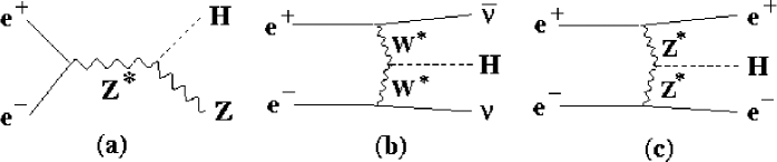
Figure 2.3: Diagrams of CP-even higgs production expected at JLC phase-I in (a) Higgs-strahlung (Bijorken) $\mathrm{h}^{0}$$\mathrm{Z}^{0}$ production, (b) WW-fusion and (c) ZZ-fusion process.

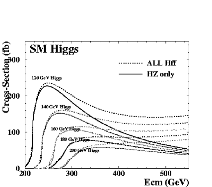
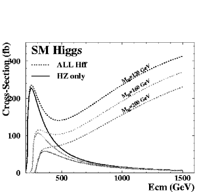
Figure 2.4: Production cross-section of the SM Higgs. (Left) The production cross-section of $\mathrm{h}^{0}$$\mathrm{Z}^{0}$ process (solid lines), and all $\mathrm{h}^{0}$$\mathrm{f}\bar{\mathrm{f}}$ process including fusion processes (dotted lines) for 120–200 GeV SM Higgs as a function of the center-of-mass energy in the range for the JLC phase-I. (Right) The cross-section for wider range in center-of-mass energies.

In the SM Higgs, the production cross-section is completely determined for a given Higgs boson mass. No free parameter exists except for the Higgs boson mass itself. Figure 2.4 shows the production cross-section. With a naive calculation we have approximately $10^{5}$ Higgs events in 5 years for 120 GeV Higgs if we have the luminosity of 10³⁴ cm^-2s^-1, with 10⁷ seconds running per year. Note that the current JLC design expects to have much larger duty factor (live running-time).

For the MSSM, the production cross-section of the $\mathrm{h}^{0}$$\mathrm{Z}^{0}$ process $\sigma_{\mathrm{hZ}}^{\mathrm{MSSM}}$ can be written as $\sigma_{\mathrm{hZ}}^{\mathrm{MSSM}}={\mathrm{sin}}^{2}(\beta-\alpha)\times\sigma_{\mathrm{HZ}}^{\mathrm{SM}}$, where $\sigma_{\mathrm{HZ}}^{\mathrm{SM}}$ is the SM Higgs cross-section. The $\beta$ is defined by tan$\beta$=$v_{1}/v_{2}$, the ratio of the vacuum expectation values of two Higgs field doublets. The $\alpha$ is the mixing angle of the two CP-even Higgs states. Note that the $\alpha$ and $\beta$ are related in the MSSM in terms of CP-odd Higgs boson (A⁰) mass and other SUSY parameters. In more general SUSY Higgs models such as NMSSM, the cross-section depends on more parameters. However, there exist absolute lower limits of the cross-section ($\sigma_{\mathrm{minimum}}$). Figure 2.5 shows the $\sigma_{\mathrm{minimum}}$ as a function of center-of-mass energy of ${\mathrm{e}}^{+}{\mathrm{e}}^{-}$ collision for the NMSSM, taken from Ref. [11], which is valid also for the MSSM Higgs.

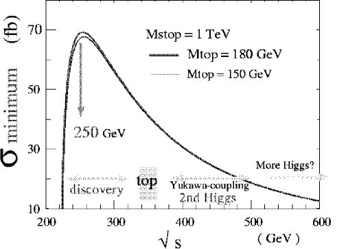
Figure 2.5: The minimum cross-section of the CP-even Higgs production in the NMSSM calculated by Y. Okada et al [11]. The two lines correspond to the top quark mass of 150 and 180 GeV.

The other Higgs expected in the multi Higgs models such as MSSM might be discovered even in the first phase of JLC project at $\sqrt{s}$ lower than 500 GeV. The one of the important measurements would be $\mathrm{A}^{0}$ ($\mathrm{H}^{0}$) production radiated off the $b$ quark or top quark, for example ${\mathrm{e}}^{+}{\mathrm{e}}^{-}$$\rightarrow$$\mathrm{t}\bar{\mathrm{t}}$$\rightarrow$$\mathrm{t}\bar{\mathrm{t}}$$\mathrm{A}^{0}$, via Yukawa-coupling. Also other channels with multi-Higgs production could be observed via Higgs self-coupling. The strategy and scenario at the next step depend on the results of the first phase. For MSSM (or general two Higgs doublets scenario), there is an additional important channel, which is ${\mathrm{e}}^{+}{\mathrm{e}}^{-}$$\rightarrow$$\mathrm{A}^{0}$$\mathrm{h}^{0}$. However, if we stick to the MSSM, the production cross-section of the $\mathrm{A}^{0}$$\mathrm{h}^{0}$ process is expected to be considerably small, if the $\mathrm{h}^{0}$ mass exceed 110 GeV, where LEP-II sensitivity ends. The heavier Higgs such as $\mathrm{A}^{0}$ and $\mathrm{H}^{0}$ would be the essential subjects to be investigated at later stage of JLC phase-I ($\sqrt{s}>350$ GeV), the second phase of the JLC at $\sqrt{s}$ higher than 500 GeV, and/or $\gamma\gamma$ option of the JLC (see Chapter IV).

2.3.2 Higgs Decay

The decay branching ratio of the SM Higgs is shown in figure 2.6. The Higgs boson couples to mass of the particle (coupling determines mass of the particle via Higgs mechanism). In the SM, coupling with fermion, namely Yukawa coupling, is m${}_{f}/v$ and M${}_{g}^{2}/v$ with weak gauge bosons where m_f, M_g are fermion mass and W or Z masses, respectively, and $v$ is the vacuum expectation value $v\approx$246 GeV. If the Higgs is of the SM like, the dominant decay branch is $\mathrm{b}\bar{\mathrm{b}}$ for Higgs mass of lighter than 130 GeV. However, once the decay channel into W pair open, the most of the Higgs is expected to decay to W pair. The decay of the MSSM Higgs depends also on $\alpha$ and $\beta$. For the first target mass region between 100 and 140 GeV where we expect the lightest Higgs in MSSM and NMSSM, again the $\mathrm{b}\bar{\mathrm{b}}$ branch dominates in wide range of the parameter space. A good b-flavour tagging is one of the essential techniques to discover and precisely measure the Higgs boson.

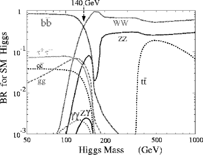
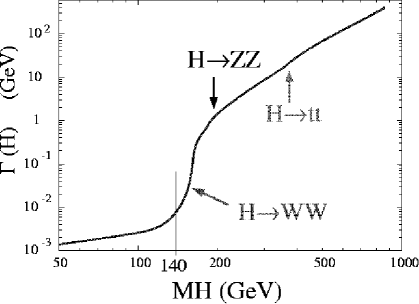
Figure 2.6: The branching ratio (Left) and the total decay width (Right) of the SM Higgs as functions of the Higgs mass.

2.3.3 Physics Backgrounds

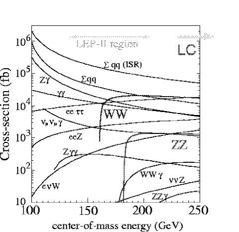
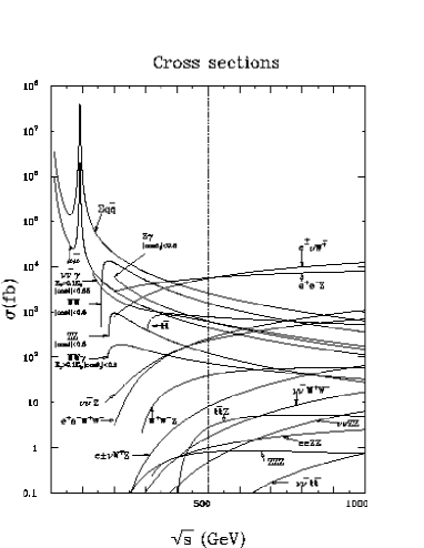
Figure 2.7: Cross-section of the physics background as a function of center-of-mass energy up to 1 TeV.

Figure 2.7 shows the cross-section of the SM background processes at energies of LEP-II and JLC region. For example, at $\sqrt{s}=300$ GeV, the dominant backgrounds are; $\mbox{$\mathrm{q}\bar{\mathrm{q}}$}(\gamma)$ (35 pb), $\mathrm{W}^{+}\mathrm{W}^{-}$ (17 pb), $\mathrm{Z}^{0}$$\mathrm{Z}^{0}$ (1.0 pb) We$\nu$ (2.0 pb), and $\mathrm{Z}^{0}$${\mathrm{e}}^{+}{\mathrm{e}}^{-}$ (1.2 pb). Once the center-of-mass energy exceeds the top-quark pair threshold, the process ${\mathrm{e}}^{+}{\mathrm{e}}^{-}$$\rightarrow$$\mathrm{t}\bar{\mathrm{t}}$ also contributes as one of the main background. At $\sqrt{s}\approx 350$ GeV, ${\mathrm{e}}^{+}{\mathrm{e}}^{-}$$\rightarrow$$\mathrm{t}\bar{\mathrm{t}}$ cross-section is approximately 0.7 pb (see Chapter4).

The $\mbox{$\mathrm{q}\bar{\mathrm{q}}$}(\gamma)$ background is relatively easy to be reduced by analyses in the event topology. The most severe background is the W pair production. In case mass of the Higgs boson is close to $m_{\mathrm{Z}}$, the ${\mathrm{e}}^{+}{\mathrm{e}}^{-}$$\rightarrow$$\mathrm{Z}^{0}$$\mathrm{Z}^{0}$ process with heavy flavour or tau lepton in the final states could be irreducible backgrounds while angular distribution can help to reduce the contamination. The situation is much better than LHC where several order of magnitude higher background level is expected and the systematical control of the background is difficult. However our ultimate purpose of the Higgs study is not only the Higgs discovery, but also to measure the Higgs properties precisely, in order to determine the direction of the future physics. The requirements of the purity and accuracy are far beyond those at LHC. Note that the physics background can be strongly suppressed furthermore by the polarized beam option [27], which is one of the big advantages of the linear collider.

2.4 Experimental Considerations

At JLC phase-I, the numbers of essential programs are waiting for us in the Higgs studies. In order to evaluate the experimental feasibilities, we use a model detector, i.e. JLC-I design. The details of JLC-I detector and its simulation methods are found elsewhere in this report. The detector has the expected performance high enough to satisfy the most of the requirements of the Higgs measurements as follows;

• Good energy measurements of charged tracks, neutral particles, and jets, in order to reconstruct Higgs boson mass.

• Precise positioning of the primary and the secondary vertices in order to tag the b-quark and c-quark from Higgs decay. The primary vertex resolution is good enough at LC since the beam size of less than $\mu$m is used in the primary vertex fitting. To establish the Higgs tagging with more than 80 % for $\mathrm{b}\bar{\mathrm{b}}$ decay with reasonable purity against background process we need to tag the secondary vertex with its decay length less than 1 mm. Furthermore, the c-quark tagging might require more accuracy. The dominant part of the charged particle from the b-hadron decay have its momentum less than 3 GeV. The detector is required to have less materials in vertex detectors.

• Good hermeticity of the detector. It is essential especially for the neutrino channel, $\mbox{${\mathrm{e}}^{+}{\mathrm{e}}^{-}$}\mbox{$\rightarrow$}\mbox{$\mathrm{h}^{0}$}\nu\bar{\nu}$. It is also important for detection of Higgs decay to W-pair for the $\mathrm{h}^{0}$$\rightarrow$WW${}^{(*)}\mbox{$\rightarrow$}$l$\nu$q$\bar{\mathrm{q}}$ events.

• Particle identification especially for leptons. The $\tau$-identification performance is one of the keys for the Higgs studies. A fine segmentation of the calorimetry with enough neutral hadron/$\gamma$ discrimination might help.

Here we review the detector performance expected at JLC phase-I based on the simulation studies of the detector. We show energy-momentum measurement for jets and leptons, and heavy flavour tagging such as b-tagging, which are crucial in the light Higgs studies, based on the preliminary simulation studies with the current JLC-I detector as a basic model.

2.4.1 Jet Energy Momentum Measurements

The one of the keys of the Higgs studies is the jet energy measurements. In most of the cases, the Higgs is expected to decay hadronically. Jet energies are measured by the central tracker system and calorimeters. The $\gamma$’s mainly from $\pi^{0}$ decay and long-lived neutral hadrons such as neutrons and K${}_{L}^{0}$ are measured by the calorimetry. Charged particles are detected both by trackers and calorimetry. In order to obtain the good resolution, the double counting in the detectors are suppressed using the information of the geometrical matching between tracks and clusters in the calorimetry systems. The double counting suppression is the one of the essential techniques for the Higgs study. The method to achieve the best jet-energy resolution (energy-flow calculation) is under development and open for the future studies.

Figure 2.8 shows the reconstructed mass distribution with JLC-I simulation with the current energy-flow calculation for Higgs signals in $\mbox{${\mathrm{e}}^{+}{\mathrm{e}}^{-}$}\mbox{$\rightarrow$}\nu\bar{\nu}\mbox{$\mathrm{h}^{0}$}\mbox{$\rightarrow$}\nu\bar{\nu}\mbox{$\mathrm{c}\bar{\mathrm{c}}$}$, $\nu\bar{\nu}gg$(gluons) and $\nu\bar{\nu}\mbox{$\mathrm{b}\bar{\mathrm{b}}$}$. For the plot, the visible masses without rescaling or kinematic fit are used. The bottom lego plot shows the correlation between missing mass, which corresponds to $\mathrm{Z}^{0}$ mass due to missing neutrino from Z decay, and the visible mass corresponding to Higgs boson mass. The reason why the $\mathrm{b}\bar{\mathrm{b}}$ decay has wider resolution is mainly due to additional neutrinos in b-hadron semi-leptonic decays.

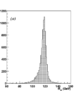
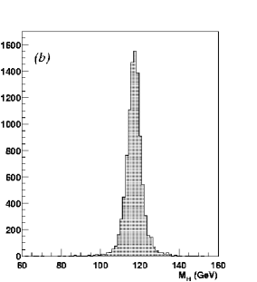
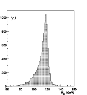
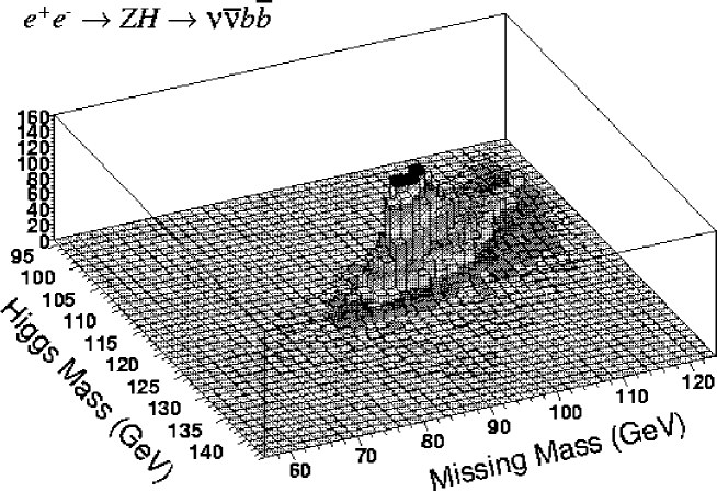
Figure 2.8: The visible mass distribution of the process $\mbox{${\mathrm{e}}^{+}{\mathrm{e}}^{-}$}\mbox{$\rightarrow$}\nu\bar{\nu}\mbox{$\mathrm{h}^{0}$}\mbox{$\rightarrow$}\nu\bar{\nu}\mbox{$\mathrm{c}\bar{\mathrm{c}}$}$ (a), $\nu\bar{\nu}\mbox{$\mathrm{h}^{0}$}\mbox{$\rightarrow$}\nu\bar{\nu}gg$ (b) and $\mbox{${\mathrm{e}}^{+}{\mathrm{e}}^{-}$}\mbox{$\rightarrow$}\nu\bar{\nu}\mbox{$\mathrm{h}^{0}$}\mbox{$\rightarrow$}\nu\bar{\nu}\mbox{$\mathrm{b}\bar{\mathrm{b}}$}$ (c) reconstructed in detector simulation for 120 GeV Higgs. The bottom plot shows the correlation between visible mass and the missing mass.

2.4.2 Lepton Momentum Measurements

In the Higgs-strahlung process, the leptonic decay (${\mathrm{e}}^{+}{\mathrm{e}}^{-}$ or $\mu^{+}\mu^{-}$) in the associated Z boson plays a special role. The channels are the most clean ones in all final states of $\mathrm{h}^{0}$$\mathrm{Z}^{0}$. Event-topology for the signal is high energy ${\mathrm{e}}^{+}{\mathrm{e}}^{-}$ or $\mu^{+}\mu^{-}$ with the invariant mass of lepton pair similar to Z. Although the branching ratio in the Z decay to ${\mathrm{e}}^{+}{\mathrm{e}}^{-}$ or $\mu^{+}\mu^{-}$ is limited ($\sim 6$%), the background similar to the signal is only those of the ${\mathrm{e}}^{+}{\mathrm{e}}^{-}$$\rightarrow$$\mathrm{Z}^{0}$$\mathrm{Z}^{0}$$\rightarrow$${\mathrm{e}}^{+}{\mathrm{e}}^{-}$X or $\mu^{+}\mu^{-}$X. Recoil mass of the two leptons corresponds to the Higgs mass without dilution by the Z natural width. The recoil mass distributions of ${\mathrm{e}}^{+}{\mathrm{e}}^{-}$$\rightarrow$$\mu^{+}\mu^{-}$X simulated with JLC-I detector for background and signal is found in Figure 2.9.

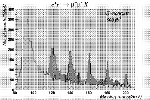
Figure 2.9: The distribution of the recoil mass of $\mu^{+}\mu^{-}$ pair in ${\mathrm{e}}^{+}{\mathrm{e}}^{-}$$\rightarrow$$\mu^{+}\mu^{-}$X normalized to 500 fb^-1 at $\sqrt{s}=300$ GeV. The background of Z-pair production process, ${\mathrm{e}}^{+}{\mathrm{e}}^{-}$$\rightarrow$$\mathrm{Z}^{0}$$\mathrm{Z}^{0}$$\rightarrow$$\mu^{+}\mu^{-}$X, and the SM Higgs boson signals of 120, 140, 160, 180 and 200 GeV are shown. The full simulation program JIM (see Chapter 12) is uses for the simulation.

2.4.3 Heavy Flavour Tagging

As we have discussed, if the Higgs boson has mass of less than 140 GeV, the dominant decay mode is expected to be $\mathrm{b}\bar{\mathrm{b}}$. Hence the b-flavour tagging is the essential technique in the light Higgs study. Figure 2.10 shows a schematic view of the cascade decay of the b-hadron. The b-hadron tends to decay sequentially to c-hadron and to hadrons with strangeness. The lifetime of the b-hadron is long enough ($\beta\gamma c\tau\sim$3–5 mm) to be observed as a displaced vertex in the detector.

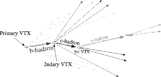
Figure 2.10: Schematic view of the cascade decay of the b-hadron (Left) and the scheme of the definition of the impact parameters (Right) for the heavy-flavour tagging.

At JLC, the position resolution of the initial production of an event (primary vertex) is expected to be much better than that of LEP, since the beam size of less than $\mu$m at JLC can be used as constraints of the primary vertex fitting. Several properties of the $\mathrm{b}\bar{\mathrm{b}}$ decay of the Higgs signal can be seen in Figure 2.11. The dominant part of the charged particle from the b-hadron decay have its momentum less than 3 GeV. Hence the low momentum track is important for the efficient Higgs tagging. One can see, to establish the Higgs tagging with more than 80 % for $\mathrm{b}\bar{\mathrm{b}}$ decay, we need to tag the secondary vertex for that with decay length less than 1 mm. In order to purify the b against c-quarks, the vertex mass and tagging of the 3rd vertex are powerful. The distance between b and c decay in a decay sequence is also less than 1 mm as shown in the figure. Kinematics of the jet and vertex is also the discriminatories of the b-hadron against lighter flavours. The b-hadron tends to decay with large multiplicity and large jet invariant mass due to heavy mass of the b-quark.

The distributions of the obtained normalized impact parameter, impact parameter divided by the expected resolution, are shown in the bottom-left plot. In the plot, the distributions for the tracks from the b-hadrons decay in the Higgs event and those from the charm hadron in the W-decay are seen, together with the distribution for the tracks produced at the primary vertex. Note that the track fitting has been made with the correct association of the hits, hence no effects of the mis-assignment of the hits are included.

There are many methods for efficient b-tagging developed and used in the experiments so far. SLD experiment at SLC extensively uses the combined information of the vertex decay length and its mass (SLD mass tagging). At LEP, sophisticated methods combining several discriminant variables are used. For example OPAL experiment uses tagging based on long lifetime combined in a likelihood method with high $p_{t}$ lepton tagging and jet kinematics. The feature of the tagging methods can be seen in Ref. [13].

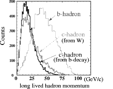
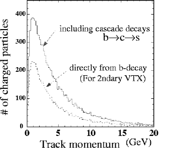
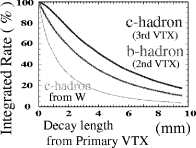
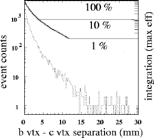
Figure 2.11: Properties of the b and c-hadrons and decay products from Higgs boson and background W pair production: (a) The momentum distribution of the heavy-flavour hadrons. (b) Distributions of the track momentum originating the b-hadron decay. (c) Distributions of decay length (the distance from the event production point to the decay point. (d) Rate (tagging efficiency) in integration of events as a function of the cut position of the decay length from the event production point.

Figure 2.12 shows the performances expected with the JLC-I detector with simulations. The left plot shows the expected impact parameter distribution for the signal process and background process of W-pair production. The right plot shows the results obtained for the impact parameter resolution for each flavour of the decay from the Higgs.

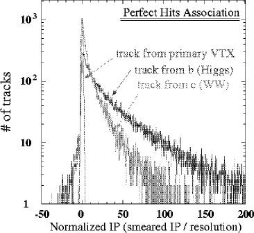
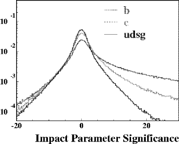
Figure 2.12: Performances obtained in the smearing simulation.

2.5 Experimental Overview; Higgs Detection and Measurement

The essential measurements of the Higgs is the mass and the coupling to other particles and to Higgs particle itself. These can be achieved by the precise measurements of the Higgs production and the decay. The key measurements at the first phase of the JLC would be as follows;

• Mass of the Higgs.

• Production and decay angular distribution and their correlations.

• Cross-section in $\mathrm{Z}^{0}$$\mathrm{h}^{0}$ and WW-fusion as a function of $\sqrt{s}$ with/without polarized beam.

• Branching ratio to $\mathrm{b}\bar{\mathrm{b}}$ (Br($\mathrm{h}^{0}$$\rightarrow$$\mathrm{b}\bar{\mathrm{b}}$)).

• Br($\mathrm{h}^{0}$$\rightarrow$$\mathrm{W}^{+}\mathrm{W}^{-}$).

• Br($\mathrm{h}^{0}$$\rightarrow$$\tau^{+}\tau^{-}$)/Br($\mathrm{h}^{0}$$\rightarrow$$\mathrm{b}\bar{\mathrm{b}}$).

• Br($\mathrm{h}^{0}$$\rightarrow$$\mathrm{c}\bar{\mathrm{c}}$)/Br($\mathrm{h}^{0}$$\rightarrow$$\mathrm{b}\bar{\mathrm{b}}$), Br($\mbox{$\mathrm{h}^{0}$}\mbox{$\rightarrow$}gg$)/Br($\mathrm{h}^{0}$$\rightarrow$$\mathrm{b}\bar{\mathrm{b}}$), Br($\mbox{$\mathrm{h}^{0}$}\mbox{$\rightarrow$}\mbox{$\mathrm{c}\bar{\mathrm{c}}$}+gg)$)/Br($\mathrm{h}^{0}$$\rightarrow$$\mathrm{b}\bar{\mathrm{b}}$).

The important thing is that we can establish/measure the properties of the Higgs particle model-independently in following things:

• Mass, which is final inputs in the SM.

• Establishment of quantum numbers (CP, spin) and s-channel production of $\mathrm{h}^{0}$$\mathrm{Z}^{0}$ final states through angular distributions and/or energy-scan

• Establish the Z mediation in $\mathrm{h}^{0}$$\mathrm{Z}^{0}$ production with polarized beam option

• SU(2)$\times$U(1) universality of HZZ and HWW comparing $\mathrm{h}^{0}$$\mathrm{Z}^{0}$ production and $\mbox{$\mathrm{h}^{0}$}\nu\bar{\nu}$ production which contains WW-fusion process.

• Absolute strength of gauge coupling to Z and to W via cross-section measurements.

• Total decay width of Higgs which is significantly sensitive to SUSY via Higgs decay branching ratio into W or Z together with the measured absolute strength of the coupling between Higgs and weak bosons.

• Absolute strength of Yukawa couplings to quarks and leptons via branching ratio to fermions together with the measured total decay width. The feasible flavour is b, c quarks, and tau.

• Self-coupling via multi Higgs production either in ${\mathrm{e}}^{+}{\mathrm{e}}^{-}$$\rightarrow$$\mathrm{Z}^{0}$$\mathrm{h}^{0}$$\mathrm{h}^{0}$ and/or $\mbox{${\mathrm{e}}^{+}{\mathrm{e}}^{-}$}\mbox{$\rightarrow$}\nu\bar{\nu}\mbox{$\mathrm{h}^{0}$}\mbox{$\mathrm{h}^{0}$}$.

In addition to these, top Yukawa coupling is measured directly from a measurement of the process ${\mathrm{e}}^{+}{\mathrm{e}}^{-}$$\rightarrow$$\mathrm{t}\bar{\mathrm{t}}$$\rightarrow$$\mathrm{t}\bar{\mathrm{t}}$$\mathrm{h}^{0}$. In case we neglect the new particle (such as SUSY) loops, the decay branching to gluons are also used to determine the top Yukawa coupling assuming the dominant contribution is a top quark loop. In other words the comparison between top Yukawa coupling and gluonic decay measures new particles with QCD color charge.

2.5.1 Discovery Potential and Sensitive Signal Cross-Section

In order to demonstrate the clean experimental environment compared to Hadron colliders, we first describe the Higgs discovery potential.

$\mathrm{h}^{0}$$\mathrm{Z}^{0}$ Production

In the e⁺e^- collider, the Higgs signal is cleanly identified. The Higgsstrahlung production process is the most clean channel to be sought. In the $\mathrm{Z}^{0}$$\mathrm{h}^{0}$ production, the event topologies are categorized by the final state of the associated $\mathrm{Z}^{0}$ boson, namely $\mathrm{q}\bar{\mathrm{q}}$, $\tau^{+}\tau^{-}$, $\nu\bar{\nu}$, ${\mathrm{e}}^{+}{\mathrm{e}}^{-}$ and $\mu^{+}\mu^{-}$.

One of the realistic estimates of the detector effects for Higgs hunt would be made by a simulation study of existing detector known to precisely follow the detector responses, while the expected performance of the detector at JLC is much better than that of the old detectors. Full simulation code of the OPAL detector at LEP was used to simulate the SM physics at center-of-mass energy of 250 GeV together with 120 GeV Higgs. The tagging of the Higgs event uses the energy-flow and b-tagging algorithms actually used in the OPAL physics at LEP-II including Higgs searches. The figure 2.13 shows the reconstructed mass distribution for the events after selection. The effective cross-section after the selection is 28.2 fb for the signal in the mass window indicated in Figure 2.13. The background has been reduced to 7.2 fb after the selection. At a glance, even with the integrated luminosity of 1 fb^-1, which corresponds to only about one day (or shorter) running of JLC, we can discover Higgs easily, even with the performance of the detector at LEP.

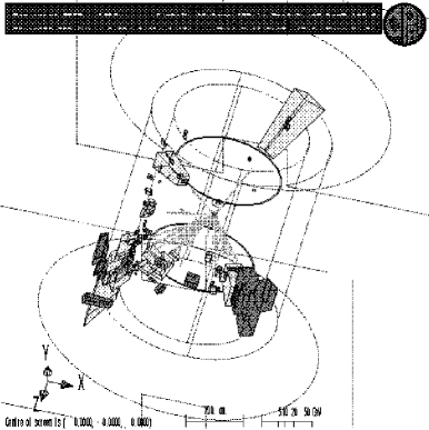
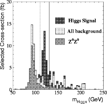
Figure 2.13: Demonstration of Higgs hunt with OPAL detector at $\sqrt{s}=250$ GeV. The SM Higgs of 120 GeV is assumed.

At JLC, in order to definitely answer to the existence of the light Higgs predicted by the SM and SUSY, we must have the sensitivity down to $\sigma\sim 10$ fb level which is one order of magnitude less than that of the SM Higgs. Once we know the efficiency and recoil mass distribution after a selection for backgrounds and a signal at certain mass, we can easily estimate the discovery sensitivity.

As an example the sensitivity is studied at 300 GeV, which is the early stage of the JLC phase-I using the JLC quick simulator. Figure 2.14 shows the discovery sensitivity for 500 fb^-1 in channels.

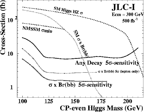
Figure 2.14: JLC-I sensitivity for the CP-even Higgs: Production cross-section sensitive at JLC-I at 300 GeV with 500 fb^-1 at more than 5$\sigma$ are shown as a function of the Higgs mass, with and without b-flavour tagging for the Higgs decay products. The line indicated by “Any decay 5$\sigma$ sensitivity” shows the JLC-I sensitivity only with leptonic channel ${\mathrm{e}}^{+}{\mathrm{e}}^{-}$$\rightarrow$$\ell^{+}\ell^{-}$$\mathrm{h}^{0}$ independent to decay of the Higgs. The cross-section for the SM Higgs, minimum cross-section for NMSSM are also shown to be compared. To compare the sensitivity for exclusive channel $\mathrm{h}^{0}$$\rightarrow$$\mathrm{b}\bar{\mathrm{b}}$ for $\sigma\times$Br($\mathrm{h}^{0}$$\rightarrow$$\mathrm{b}\bar{\mathrm{b}}$), the SM Higgs $\sigma\times$Br($\mathrm{h}^{0}$$\rightarrow$$\mathrm{b}\bar{\mathrm{b}}$), and expected sensitivity at JLC are also shown.

We first check the simplest mode, ${\mathrm{e}}^{+}{\mathrm{e}}^{-}$$\rightarrow$$\mathrm{h}^{0}$$\mathrm{Z}^{0}$ and $\mathrm{Z}^{0}$$\rightarrow$${\mathrm{e}}^{+}{\mathrm{e}}^{-}$ or $\mu^{+}\mu^{-}$. These channels are only 6% of the produced $\mathrm{h}^{0}$$\mathrm{Z}^{0}$ due to the branching ratio of the Z. The $\mathrm{Z}^{0}$$\mathrm{Z}^{0}$ process is almost all the background. Only the recoil mass is used in the analysis in order to have the sensitivity independent to the decay of the Higgs. As shown in the figure, we are sensitive up to more than 200 GeV for the CP-even Higgs with cross-section similar to the SM model even at $\sqrt{s}=300$ GeV only from the lepton spectra independent to decay of the Higgs.

When we utilize the b-tagging, we can suppress the huge background from $\mathrm{W}^{+}\mathrm{W}^{-}$ production, which enables us to use hadronic decay of Z, $\mathrm{h}^{0}$$\mathrm{Z}^{0}$$\rightarrow$$\mathrm{h}^{0}$$\mathrm{q}\bar{\mathrm{q}}$, which carries 70% (Br($\mathrm{Z}^{0}$$\rightarrow$$\mathrm{q}\bar{\mathrm{q}}$)) of the $\mathrm{h}^{0}$$\mathrm{Z}^{0}$ signal process. While the signal of $\mathrm{h}^{0}$$\mathrm{Z}^{0}$$\rightarrow$$\mathrm{b}\bar{\mathrm{b}}$$\mathrm{Z}^{0}$ also reduces the efficiency, the sensitivity to $\sigma\times$Br($\mathrm{b}\bar{\mathrm{b}}$) reaches down to less than 2 fb as shown in the figure.

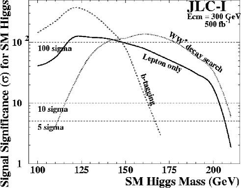
Figure 2.15: Higgs signal significance for the SM Higgs in $\mathrm{H}^{0}$$\mathrm{Z}^{0}$ channels: Three methods are shown; 1) only lepton channel independent to Higgs decay, 2) using b-tagging enrich $\mathrm{h}^{0}$$\rightarrow$$\mathrm{b}\bar{\mathrm{b}}$ signal expected for light Higgs, and 3) analysis optimized for $\mbox{$\mathrm{h}^{0}$}\mbox{$\rightarrow$}\mbox{$\mathrm{W}^{+}\mathrm{W}^{-}$}^{*}$ decay.

The luminosity necessary to discover the SM Higgs is shown in Figure 2.16 as a function of the SM Higgs mass. Note that the data correspond to 1 fb^-1 is expected to be accumulated in less than one day at the JLC.

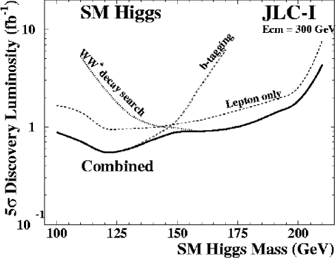
Figure 2.16: Integrated luminosity necessary to discover (5$\sigma$) the SM Higgs at JLC phase-I $\sqrt{s}=300$ GeV. Luminosity of 1 fb^-1 correspond to about “one day” running at JLC.

$\mathrm{A}^{0}$$\mathrm{h}^{0}$ Production

Let’s consider the two Higgs field doublets (2HDM) type-II including MSSM. We assume here CP conservation in the Higgs sector. We have 5 physical states, two CP-even $\mathrm{h}^{0}$ and $\mathrm{H}^{0}$, CP-odd $\mathrm{A}^{0}$ and positively and negatively charged Higgs. $\mathrm{A}^{0}$ mass is unknown and possible mass is from 90 to 2 TeV or more in the MSSM. CP-odd nature of $\mathrm{A}^{0}$ inhibits the decay to pair of gauge bosons. In general $\mathrm{A}^{0}$ decay to heavy quarks in wide range of 2HDM parameters. Kinematical accessible mass is $\mbox{$m_{\mathrm{A}}$}<\sqrt{s}-\mbox{$m_{\mathrm{h}}$}$, hence we have a potential to produce $\mathrm{A}^{0}$$\mathrm{h}^{0}$ in the case such as $\mbox{$m_{\mathrm{h}}$}=120$ GeV, $\mbox{$m_{\mathrm{A}}$}=300$ GeV at $\sqrt{s}=500$ GeV. At that time, the CP-even light Higgs is measured already by $\mathrm{h}^{0}$$\mathrm{Z}^{0}$ production at JLC. For the branching ratio of $\mathrm{h}^{0}$ to $\mathrm{b}\bar{\mathrm{b}}$, we assume 70%. In this benchmark case, $\mathrm{A}^{0}$ cannot decay to top quark, and we assume here the decay to $\mathrm{b}\bar{\mathrm{b}}$ has branching ratio more than 80%. The production cross-section depends on tan$\beta$ and $\alpha$. The analysis can be made in two steps; the first clean four jet topology with b quark signature in all jets to be selected, then next choose a jet-pair which corresponds to CP-even Higgs mass. The other jets are combined to measure $\mathrm{A}^{0}$ mass.

The dominant backgrounds are; 1) $\mathrm{Z}^{0}$$\mathrm{Z}^{0}$ process with b-quark decay of both Z, 2) $\mathrm{b}\bar{\mathrm{b}}$ production together with multi hard gluon radiation followed by b production, 3) top-quark pair production followed by $\mathrm{t}\bar{\mathrm{t}}$$\rightarrow$bWbW$\rightarrow$bqqbqq, and 4) production of $\mathrm{h}^{0}$ signal itself in the Higgsstrahlung process. The top quark pair and $\mathrm{b}\bar{\mathrm{b}}$ backgrounds are suppressed by its event topology and four b quark requirement. The $\mathrm{Z}^{0}$$\mathrm{Z}^{0}$$\rightarrow$$\mathrm{b}\bar{\mathrm{b}}$$\mathrm{b}\bar{\mathrm{b}}$ background is further suppressed by a veto for the events which corresponds to ZZ in a jet combination. Finally the jet pair mass is checked if the accumulation exist compared to background. The selection efficiency for the process is 20% with selected background cross-section of about 0.05 fb from non-Higgs background. The most sever background might be Higgsstrahlung signal itself. It corresponds to about 0.1 fb if the $\mathrm{h}^{0}$ is of SM-like (sin${}^{2}(\alpha-\beta)\sim 1$). At 1000 fb^-1, we have 50 event non-Higgs background and 100 events from Higgsstrahlung in the mass window. It means 5$\sigma$ corresponds to signal cross-section of about 0.4 fb.

If we have a sensitivity down to 0.4 fb, we can estimate the sensitivity to cos²($\alpha-\beta$) in $m_{\mathrm{h}}$-$m_{\mathrm{A}}$ plane. In all cases, $\mathrm{h}^{0}$ is assumed to be SM-like in order to check the sensitivity to cos²($\alpha-\beta$), hence SM Br is used for $\mathrm{h}^{0}$.

Yukawa Production of $\mathrm{h}^{0}$, $\mathrm{A}^{0}$

The cross-section for the SM Higgs is shown in figure??? for the processes ${\mathrm{e}}^{+}{\mathrm{e}}^{-}$$\rightarrow$$\mathrm{t}\bar{\mathrm{t}}$$\rightarrow$$\mathrm{t}\bar{\mathrm{t}}$$\mathrm{H}^{0}$ and ${\mathrm{e}}^{+}{\mathrm{e}}^{-}$$\rightarrow$$\mathrm{b}\bar{\mathrm{b}}$$\rightarrow$$\mathrm{b}\bar{\mathrm{b}}$$\mathrm{H}^{0}$ for $\sqrt{s}=$500, and 1000 GeV as a function of the SM Higgs mass. The measured error $\Delta\sigma/\sigma$ linearly depend on the inverse of the square root of the cross-section times the integrated luminosity, in case the background is negligible. The sensitive cross-section is about 0.1 fb for 1000 fb^-1.

2.5.2 Mass Measurements

The Higgs boson mass is the fundamental value which might give us information up to GUT scale as we discussed above. A precise measurement of the Higgs mass with an accuracy of about 100 MeV or less is necessary in order to obtain fruitful results from the other measurements such as branching ratio especially for Higgs around 120–150 GeV. The Higgs branching ratio is a strong function of its mass mainly due to kinematic phase space factor of Higgs decay into W-pair.

The Higgs mass can be obtained either with direct reconstruction of the jets from Higgs, or with recoil mass in case the associated Z⁰ decays to e⁺e^- or $\mu^{+}\mu^{-}$, or with all information combined with fitting with energy-momentum (and $\mathrm{Z}^{0}$ mass) constraints. It can be compared to the W boson mass measurement ($\Delta m\sim 40$ MeV) at LEP using the similar technique of the event-by-event direct reconstruction with about 50000 WW events in LEP which is approximately the same order as the expected Higgs signal. What is different with WW measurements at LEP and Higgs mass measurement at JLC are;

• wider beam energy spread ($\sim 0.5$%)

• better detector resolution

• smaller (negligible) natural width of Higgs

• precise knowledge of Z mass can be used

Precise calibration of the detector and beam energy measurement are essential as of W mass measurement. Calibration runs at $\mathrm{Z}^{0}$ pole might be helpful [28]. It should be noted that the actual e⁺e^- collision energy has a relatively large spread in linear colliders compared to circular colliders like LEP. Also there we expect significant beamstrahlung effect [21] in exchange for the high luminosity. These make a distortion of the reconstructed Higgs mass as well as the background processes when we use the beam energy constraints. In case we use the recoil mass or constraint fitting, also the ISR at the physics collision affects the mass resolution if the center-of-mass energy is significantly higher than $\mbox{$m_{\mathrm{H}}$}+\mbox{$m_{\mathrm{Z}}$}$. These effects are seen in Figure 2.17 for ${\mathrm{e}}^{+}{\mathrm{e}}^{-}$$\rightarrow$$\mathrm{Z}^{0}$$\mathrm{h}^{0}$$\rightarrow$$\mu^{+}\mu^{-}$$\mathrm{h}^{0}$ for the SM Higgs with its mass of 120 GeV at $\sqrt{s}=250$ GeV.

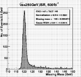
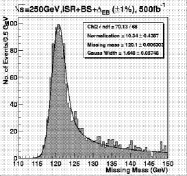
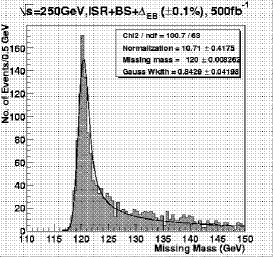
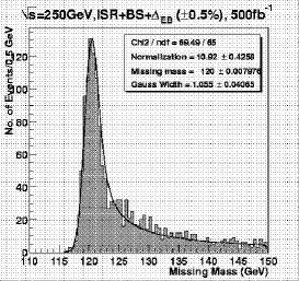
Figure 2.17: The distribution of the recoil mass of $\mu^{+}\mu^{-}$ pair in ${\mathrm{e}}^{+}{\mathrm{e}}^{-}$$\rightarrow$$\mu^{+}\mu^{-}$$\mathrm{h}^{0}$ for the 120 GeV SM Higgs normalized to 500 fb^-1 at $\sqrt{s}=250$ GeV. Different beam parameters are used.

The simplest way to determine the Higgs mass is to use lepton final state of the associated Z (lepton channel). In this case, we measure the mass of the Higgs as the recoil mass of the leptons. For the light Higgs of 120–140 GeV, our first target, we have production cross-section more than 100 fb^-1 at JLC phase-I for the SM-type Higgs. The selected event rate for the lepton channel is about 2000 events per 500 fb^-1, and the mass resolution per event is $\sim$2 GeV at 300 GeV. With design beam parameter at JLC, and including ISR, we expect 80 MeV for the precision of the mass from the lepton channels. Note that the precise calibration for the electron energy scale in detector response is important for electron channel. In order to avoid the possible bias in the energy scale, we may use the kinematic fitting.

If we utilize other channels, the statistics of the Higgs signal jumps up. In the missing energy channel, the visible mass correspond to Higgs boson. JLC detector has jet-jet invariant mass resolution of around 3 GeV for 120 GeV Higgs at 300 GeV. Hence if we know the detector energy scale precisely enough we may measure the Higgs in this channel with the similar level as leptonic channel or even less. The precision is determined by the error in the energy scale in detector. The constraints fit of the missing mass to Z does not gain. If we calibrate the detector response in jet energy scale either using Z⁰ calibration and/or energy scaling by visible energy peak to $\mathrm{Z}^{0}$ mass using $\mbox{$\mathrm{Z}^{0}$}\mbox{$\mathrm{Z}^{0}$}\mbox{$\rightarrow$}\mbox{$\mathrm{q}\bar{\mathrm{q}}$}\nu\bar{\nu}$ especially for $\mbox{$\mathrm{Z}^{0}$}\mbox{$\mathrm{Z}^{0}$}\mbox{$\rightarrow$}\mbox{$\mathrm{b}\bar{\mathrm{b}}$}\nu\bar{\nu}$, we may achieve the necessary precision.

Also we can use the four quark final states ${\mathrm{e}}^{+}{\mathrm{e}}^{-}$$\rightarrow$$\mathrm{Z}^{0}$$\mathrm{h}^{0}$$\rightarrow$$\mathrm{q}\bar{\mathrm{q}}$$\mathrm{b}\bar{\mathrm{b}}$. In this channel, the Higgs mass is in principle deducible from the jet-jet invariant mass for jets assigned to Higgs, and/or recoil mass of the jet pair associated to Z. However the jet clustering of decay products from Higgs and Z mixes each other. A possible way is to use the constraints fit or scaling with energy-momentum constraints. In this case the jet direction, which is not affected much by the mixing, can be used strongly. The mass of the Higgs is assigned event by event as $M_{12}+M_{34}-\mbox{$m_{\mathrm{Z}}$}$ where $M_{ij}$ is the jet-pair invariant mass after the fitting. It is almost equivalent to 5-constraints fitting (Z⁰ constraints for a jet pair in addition to the energy-momentum conservation). The mass resolution is governed mostly by the $\mathrm{Z}^{0}$ natural width ($\sim 2$ GeV) and the beam energy spread. In this case, again the knowledge of the absolute central beam energy and spread is essential. Also the effect of the ISR has to be controlled theoretically.

Through these measurements, we expect to be able to measure the Higgs mass within accuracy of 40 MeV assuming the central beam energy is known to less than the error, which is roughly the same size as LEP WW mass as we expected.

Note that the effects of the ISR and beamstrahlung on the mass measurement significantly depend on the center-of-mass energy. Cross-section and the momentum resolution also depend on the center-of-mass energy. The dependence of the center-of-mass energies for the Higgs mass reconstruction is shown in Figure 2.18 for the muon channel. As shown in the figure, for 120 GeV Higgs, we have a recoil mass resolution of about 0.8, 1.0 and 1.8 GeV for $\sqrt{s}=240$, 250 and 300 GeV, respectively. Once we discover Higgs, beam parameters should be re-optimized.

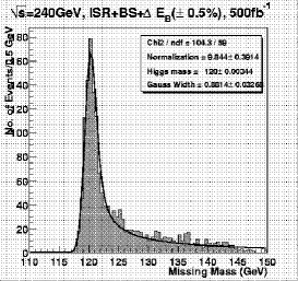
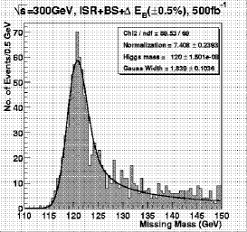
Figure 2.18: The distribution of the recoil mass of $\mu^{+}\mu^{-}$ pair in ${\mathrm{e}}^{+}{\mathrm{e}}^{-}$$\rightarrow$$\mu^{+}\mu^{-}$$\mathrm{h}^{0}$ for the 120 GeV SM Higgs normalised to 500 fb^-1 at $\sqrt{s}=240$, 250 and 300 GeV.

2.5.3 Quantum Numbers and Verification of ZZH Coupling

It is essential to verify the particle found is produced via ZZH coupling. If we establish the coupling, and verify the spin 0 scalar particle, then it is a direct evidence that the particle should have a vacuum expectation value from the requirement of gauge coupling.

The final state of ZH is considered. The verification is easily made via three steps;

1. s-channel production is verified from the production angle measurement.

2. The particle spin and parity is established also from the production angle together with the decay angle, and also from the energy scan.

3. Then finally the question if the intermediated particle is Z or not is verified for example with polarized beam option.

2.5.4 Higgs strahlung and WW(ZZ)-fusion Cross-section Measurements

The cross-section measurements of the $\mathrm{Z}^{0}$$\mathrm{h}^{0}$ (and WW-fusion) process mean the direct determination of the coupling between Higgs and weak bosons. The measurement is significantly important. If we find the cross section even slightly different from what we expect from the SM, it means we have more than one Higgs in the Universe. In MSSM or type-II 2HDM, the cross-section normalized to the SM value is sin²($\alpha-\beta$). If heavier Higgs is found in JLC or LHC, we are already able to check the MSSM using the relation between light Higgs mass, heavier Higgs mass and $\alpha-\beta$ measured above. The ZZh coupling is directly measured with Higgs-strahlung process using ${\mathrm{e}}^{+}{\mathrm{e}}^{-}$$\rightarrow$$\mathrm{q}\bar{\mathrm{q}}$$\mathrm{h}^{0}$, $\mu^{+}\mu^{-}$$\mathrm{h}^{0}$, $\tau^{+}\tau^{-}$$\mathrm{h}^{0}$ or ${\mathrm{e}}^{+}{\mathrm{e}}^{-}$$\mathrm{h}^{0}$ (with small contribution from ZZ-fusion). The neutrino channel $\mbox{${\mathrm{e}}^{+}{\mathrm{e}}^{-}$}\mbox{$\rightarrow$}\mbox{$\mathrm{h}^{0}$}\nu\bar{\nu}$ is important to measure WWh coupling via WW-fusion process [29]. The comparison between ZZh and WWh couplings verify the SU(2)$\times$U(1) structure, which is essential to establish the Higgs mechanism. Once the SU(2)$\times$U(1) coupling is established, all channels are combined to precisely determine both ZZh and WWh couplings.

HZ Cross-section measurement

As we’ve described above, in the $\mathrm{Z}^{0}$$\mathrm{h}^{0}$ production, the event topologies are categorized by the final state of the associated $\mathrm{Z}^{0}$ boson, namely $\mathrm{q}\bar{\mathrm{q}}$, $\tau^{+}\tau^{-}$, $\nu\bar{\nu}$, ${\mathrm{e}}^{+}{\mathrm{e}}^{-}$ and $\mu^{+}\mu^{-}$. In order to measure the cross-section independently of the Higgs decay branching, the simplest way is to use ${\mathrm{e}}^{+}{\mathrm{e}}^{-}$$\rightarrow$$\mathrm{Z}^{0}$$\mathrm{h}^{0}$$\rightarrow$$\mu^{+}\mu^{-}$$\mathrm{h}^{0}$ channel in the recoil mass distribution of the muon pairs. We assume HZ cross section of 200 fb which is similar to SM optimizing the beam energy, and 500 fb^-1 integrated luminosity. We have about 1500 selected signal events in the mass window with background of 400 events for 120 GeV. It corresponds to about 3% error on $\Delta\sigma/\sigma$. We add the statistics with electron channel which includes small contribution from the ZZ-fusion to be corrected. These two lepton channels already reach to 2% level. Systematic errors are the uncertainties in the selection efficiency of the signal due to acceptance such as isolation requirement of lepton and jets, that in the background and signal shapes especially due to uncertainty of the tail in the beam energy spectrum. These errors can be controlled in the data itself using similar event topology like ZZ process for which the cross-section is known already at the 1–2 % level at present, and theoretical works are in progress.

These leptonic channels have small branching compared to all $\mathrm{Z}^{0}$$\mathrm{h}^{0}$ production due to only 3 % of the branching from $\mathrm{Z}^{0}$ to each lepton flavour. Hence the inclusion of the other channels may be helpful. However the current analysis for other channels needs requirements to the Higgs decay products in order to purify the signal. Once we measure the branching ratio in dominant modes such as to $\mathrm{b}\bar{\mathrm{b}}$ (or $\mathrm{W}^{+}\mathrm{W}^{-}$ for higher mass), the other channels might also be used to determine the cross-section more precisely. In this case, however, the precision of the cross-section measurement is determined by that of the Br-measurements in this case, which is expected to be the same level. See below.

WW-fusion Cross-section measurement

The WW-fusion process is a key to establish the universality between WWH and ZZH coupling in SU(2)$\times$U(1) symmetry breaking. The WW-fusion happens for final state of $\mbox{$\mathrm{h}^{0}$}\nu\bar{\nu}$ for the electron neutrino. The interference between fusion and Higgsstrahlung is not negligible, and the cross-section for the WW-fusion process increase quite rapidly as a function of the beam energy. In this final state, $\mbox{$\mathrm{h}^{0}$}\nu\bar{\nu}$, all the visible particles are the decay products of the Higgs. The first signature of this final state is the large missing energy due to the escaping neutrino. In order to free from the Z-mediated or WW-fusion, we do not require the missing mass to be Z mass. The main background at $\sqrt{s}<350$ GeV is the WW background with leptons from a W untagged by the detector. One of the case is the lepton going inside beam pipe direction, and in case the lepton is tau with its decay products close to other jet. Detector hermeticity, lepton tagging even inside the jets, and tau tagging are essential. The visible mass of the event is the most essential.

There are many ways to investigate the $\mbox{$\mathrm{h}^{0}$}\nu\bar{\nu}$ final state for the WW fusion.

• simple counting experiment with tight selection

• shape fits in the missing mass and/or production angle

• energy-scan

• polarized beam

So far we have studied the $\mbox{$\mathrm{h}^{0}$}\nu\bar{\nu}$ signal detection in the JLC-I simulation in a simple counting experiment, using a loose b-quark tagging based on the impact parameter to further suppress the background, especially WW process. First attempt was made neglecting the interference between WW-fusion and Higgsstrahlung. The center-of-mass energy and Higgs mass are set to $\sqrt{s}$=300 GeV and $m_{\mathrm{h}}$=120 GeV. The analysis uses a standard set of cuts like acoplanarity, multiplicity. Finally a rather wide range of the mass from 100–130 GeV are sought to count the number of events.

The expected number of signal and background events are summarized in the table 2.2. A total signal selection efficiency is estimated to be $\sim$ 50 %. A statistical error of the measurement of the Higgs production cross-section times branching ratio to $\mathrm{b}\bar{\mathrm{b}}$ in $\mbox{$\mathrm{h}^{0}$}\nu\bar{\nu}$ final states including HZ and WW fusion process is found to be $\delta\sigma/\sigma$ = 1.2% at an integrated luminosity of 500 pb^-1.

Table 2.2: The expected number of signal and background events at the center of mass energy of 300 GeV, Higgs mass of 120 GeV and an integrated luminosity of 500 fb^-1 which corresponds to several years JLC running.

Process	Selected Number of Events
HZ($\nu\nu$bb)	7015
WW fusion($\nu\nu$bb)	3580
Other Higgs signal	231.5
$\mbox{${\mathrm{e}}^{+}{\mathrm{e}}^{-}$}\mbox{$\rightarrow$}\mbox{$\mathrm{q}\bar{\mathrm{q}}$}(\gamma)$	348.5
WW background	998
ZZ background	4990
We$\nu$ background	245
Zee background	150.5

An attempt was also made to suppress the Higgs strahlung with a requirement on the missing mass to be larger than 140 GeV. The 2480 events of WW fusion process are expected to pass the additional cut, while the other Higgs process events and the total backgrounds are suppressed to be 1030 and 2475, respectively. An error of the measurement of the Higgs production cross-section for WW fusion process times b-quark decay branching is obtained to be about 3.1% in this case.

The better selection using likelihood or neural network may help. In order to deduce the absolute cross-section independent to branching ratio, we again need the accurate measurement of the branching ratio to $\mathrm{b}\bar{\mathrm{b}}$ in this case as well as the accurate estimate of the signal and background selection efficiency. Fitting in shape of the missing mass and production angle may be much powerful than the method described above in order to check the contribution of the WW-fusion in $\mbox{$\mathrm{h}^{0}$}\nu\bar{\nu}$ process, since the absolute strength of the HZ process can be normalized to what we obtained by the HZ cross-section measurement in other channels mentioned above. We also have many other ways to investigate the contribution from the WW-fusion process as are mentioned above.

2.5.5 Branching Ratio Measurements

Outlook

The measurements of the branching ratio (Br-measurement) of the Higgs is one of the keys to distinguish the SM and other models such as SUSY. Once we determine the Higgs mass, the branching ratio of the SM Higgs is completely determined by the known SM parameters. On the other hand, for SUSY Higgs, the branching can be affected by other SUSY parameters such as $\mathrm{A}^{0}$ mass or tan$\beta$, which result in the different branching ratio from the SM case.

The measurements of the branching ratio (Br) of the Higgs is one of the keys to distinguish the SM from other models such as SUSY. Once we determine the Higgs mass, the branching ratios of the SM Higgs are calculable with the known SM parameters. On the other hand, for SUSY Higgs or other Higgs models, the branching can be affected by other model parameters such as $\mathrm{A}^{0}$ mass or tan$\beta$, which result in the different branching ratio from the SM.

When we assume heavy ($\sim 2$ TeV) mass for $\mathrm{A}^{0}$ and other SUSY particles, the branching ratios in MSSM are very similar to those of the SM by the decoupling theorem. There are a lot of Br-measurements. Of these the most interesting are the Br-measurement of Higgs decaying into $\mathrm{b}\bar{\mathrm{b}}$, $\tau^{+}\tau^{-}$ and $\mathrm{W}^{+}\mathrm{W}^{-}$.

When we combine the Br($\mathrm{h}^{0}$$\rightarrow$$\mathrm{W}^{+}\mathrm{W}^{-}$) with the cross-section measurement, the total width of the Higgs can be deduced. The absolute coupling of Higgs and W boson can be determined by the cross-section measurement either of $\mathrm{Z}^{0}$$\mathrm{h}^{0}$ production with SU(2)$\times$U(1) coupling assumed, or of the WW-fusion process. The partial width of the Higgs to $WW$, $\Gamma_{\mbox{$\mathrm{h}^{0}$}\mbox{$\rightarrow$}\mbox{$\mathrm{W}^{+}\mathrm{W}^{-}$}}$, is calculable from the coupling strength obtained by the cross-section measurement. It can be written as

$${\Gamma_{\mbox{$\mathrm{h}^{0}$}\mbox{$\rightarrow$}\mbox{$\mathrm{W}^{+}\mathrm{W}^{-}$}}=\Gamma_{\mbox{$\mathrm{h}^{0}$}\mbox{$\rightarrow$}\mbox{$\mathrm{W}^{+}\mathrm{W}^{-}$}}^{\mathrm{SM}}\times\frac{\sigma_{\mbox{$\mathrm{h}^{0}$}\mbox{$\mathrm{Z}^{0}$}}}{\sigma_{\mbox{$\mathrm{h}^{0}$}\mbox{$\mathrm{Z}^{0}$}}^{\mathrm{SM}}}}~{}~{}~{}~{},$$ (2.6)

where $\Gamma_{\mbox{$\mathrm{h}^{0}$}\mbox{$\rightarrow$}\mbox{$\mathrm{W}^{+}\mathrm{W}^{-}$}}^{\mathrm{SM}}$ is the partial width of the $\mathrm{h}^{0}$$\rightarrow$$\mathrm{W}^{+}\mathrm{W}^{-}$ in the SM, $\sigma_{\mbox{$\mathrm{h}^{0}$}\mbox{$\mathrm{Z}^{0}$}}$ is the production cross-section obtained in the experiment, and the $\sigma_{\mbox{$\mathrm{h}^{0}$}\mbox{$\mathrm{Z}^{0}$}}^{\mathrm{SM}}$ is that for the SM. Finally the total width of the Higgs $\Gamma_{\mbox{$\mathrm{h}^{0}$}}$ is calculated as

$${\Gamma_{\mbox{$\mathrm{h}^{0}$}}=\frac{\Gamma_{\mbox{$\mathrm{h}^{0}$}\mbox{$\rightarrow$}\mbox{$\mathrm{W}^{+}\mathrm{W}^{-}$}}}{{\mathrm{Br}}(\mbox{$\mathrm{h}^{0}$}\mbox{$\rightarrow$}\mbox{$\mathrm{W}^{+}\mathrm{W}^{-}$})}=\Gamma_{\mbox{$\mathrm{h}^{0}$}}^{\mathrm{SM}}\times\frac{{\mathrm{Br}}^{\mathrm{SM}}(\mbox{$\mathrm{h}^{0}$}\mbox{$\rightarrow$}\mbox{$\mathrm{W}^{+}\mathrm{W}^{-}$})}{{\mathrm{Br}}(\mbox{$\mathrm{h}^{0}$}\mbox{$\rightarrow$}\mbox{$\mathrm{W}^{+}\mathrm{W}^{-}$})}\times\frac{\sigma_{\mbox{$\mathrm{h}^{0}$}\mbox{$\mathrm{Z}^{0}$}}}{\sigma_{\mbox{$\mathrm{h}^{0}$}\mbox{$\mathrm{Z}^{0}$}}^{\mathrm{SM}}}}~{}~{}~{},$$ (2.7)

where $\Gamma_{\mbox{$\mathrm{h}^{0}$}}^{\mathrm{SM}}$ is the total width for the SM Higgs.

In a similar manner, the absolute strength of the Yukawa-couplings $\lambda_{f}$ of the Higgs boson to fermions can be deduced in a model independent fashion, using the relative branching ratio Br($\mathrm{h}^{0}$$\rightarrow$$\mathrm{f}\bar{\mathrm{f}}$)/Br($\mathrm{h}^{0}$$\rightarrow$$\mathrm{W}^{+}\mathrm{W}^{-}$) together with the measured cross-section.

$$\lambda_{f}^{2}=\lambda^{2}_{f,SM}\times\frac{\mathrm{BR}(\mbox{$\mathrm{h}^{0}$}\mbox{$\rightarrow$}\mbox{$\mathrm{f}\bar{\mathrm{f}}$})\cdot\sigma_{\rm HZ}\cdot\mathrm{BR}^{SM}(\mbox{$\mathrm{h}^{0}$}\mbox{$\rightarrow$}\mbox{$\mathrm{W}^{+}\mathrm{W}^{-}$})}{\mathrm{BR}^{SM}(\mbox{$\mathrm{h}^{0}$}\mbox{$\rightarrow$}\mbox{$\mathrm{f}\bar{\mathrm{f}}$})\cdot\sigma^{SM}_{\rm HZ}\cdot\mathrm{BR}(\mbox{$\mathrm{h}^{0}$}\mbox{$\rightarrow$}\mbox{$\mathrm{W}^{+}\mathrm{W}^{-}$})}~{}~{}~{}~{},$$ (2.8)

The ratio Br($\mathrm{h}^{0}$$\rightarrow$$\tau^{+}\tau^{-}$)/Br($\mathrm{h}^{0}$$\rightarrow$$\mathrm{b}\bar{\mathrm{b}}$) is also the one of the essential measurements. In SM, various SUSY, and also in more general type-II two Higgs doublets model, an universal coupling to the charged lepton and down-type quarks are assumed at tree level,
Br($\mathrm{h}^{0}$$\rightarrow$$\tau^{+}\tau^{-}$)/Br($\mathrm{h}^{0}$$\rightarrow$$\mathrm{b}\bar{\mathrm{b}}$)=$m^{2}_{\tau}/m^{2}_{b}$. While the different absolute values of the Yukawa-coupling strength are expected in models, the ratio Br($\mathrm{h}^{0}$$\rightarrow$$\tau^{+}\tau^{-}$)/Br($\mathrm{h}^{0}$$\rightarrow$$\mathrm{b}\bar{\mathrm{b}}$) is the same in the SM and type-II models. This is the key measurement to make a definite answer in the origin of the mass in the lepton sector. On the other hand, if we assume the Type-II coupling like SM or MSSM, the measurement serves as the precise measurement of the running b-quark mass at the Higgs mass. Note that the loop effects by SUSY particles especially scalar top/bottom quarks and gluinos could make a significant correction in the decay branch into quarks. Hence the measurement is one of the key to determine SUSY parameters as described later if we live in the SUSY world.

The measurements of Br($\mathrm{h}^{0}$$\rightarrow$$\mathrm{c}\bar{\mathrm{c}}$)/Br($\mathrm{h}^{0}$$\rightarrow$$\mathrm{b}\bar{\mathrm{b}}$) is also the important to measure the Yukawa-coupling for up-type quarks. Br($\mbox{$\mathrm{h}^{0}$}\mbox{$\rightarrow$}gg$)/Br($\mathrm{h}^{0}$$\rightarrow$$\mathrm{b}\bar{\mathrm{b}}$) or Br($\mbox{$\mathrm{h}^{0}$}\mbox{$\rightarrow$}\mbox{$\mathrm{c}\bar{\mathrm{c}}$}+gg)$)/Br($\mathrm{h}^{0}$$\rightarrow$$\mathrm{b}\bar{\mathrm{b}}$) are also to be used to determine the Yukawa-coupling for up-type quarks since the gluonic decay occurs mainly via the top quark loop in most of the models.

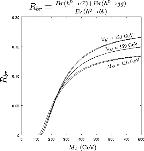
Figure 2.19: The ratio Br($\mbox{$\mathrm{h}^{0}$}\mbox{$\rightarrow$}\mbox{$\mathrm{c}\bar{\mathrm{c}}$}+gg$)/Br($\mathrm{h}^{0}$$\rightarrow$$\mathrm{b}\bar{\mathrm{b}}$) predicted by J. Kamoshita et al [30] in MSSM, as a function of the mass of the CP-odd Higgs ($\mathrm{A}^{0}$). From the top, the set of parameters $(m_{h},M_{SUSY},A_{t},\mu)$ are (130, 5000, 10000, 500), (130, 10000, 20000, 500), (120, 1000, 2000, 300), (120, 5000, 5000, 300), (110, 1000, 0, 300), and (110, 500, 750, 300) in GeV, and $\tan{\beta}$ is solved to fix $m_{h}$.

In SUSY, the gluonic decay can happen also via scalar top or scaler bottom loops, hence comparison between gluonic decay branching and Yukawa coupling to be directly measured at LHC and/or by the ${\mathrm{e}}^{+}{\mathrm{e}}^{-}$$\rightarrow$$\mathrm{t}\bar{\mathrm{t}}$$\rightarrow$$\mathrm{t}\bar{\mathrm{t}}$$\mathrm{h}^{0}$ at JLC could give us information in the scaler quark sector. The ratios relative to those of the SM are proportional to tan${}^{-2}\alpha\times$tan${}^{-2}\beta$ which can be approximated as $[(\mbox{$m_{\mathrm{A}}$}^{2}-\mbox{$m_{\mathrm{h}}$}^{2})/(\mbox{$m_{\mathrm{A}}$}^{2}-\mbox{$m_{\mathrm{Z}}$}^{2})]^{2}$ for large tan$\beta$, which leads the indirect estimation of CP-odd Higgs $\mathrm{A}^{0}$ mass [30, 31]. However one should note that the theoretical ambiguities is large due to uncertainty of $\alpha_{s}$ and running c-quark mass. Theoretical and experimental improvements are awaited.

The measurements of Br($\mathrm{h}^{0}$$\rightarrow$$\mathrm{c}\bar{\mathrm{c}}$)/Br($\mathrm{h}^{0}$$\rightarrow$$\mathrm{b}\bar{\mathrm{b}}$), Br($\mbox{$\mathrm{h}^{0}$}\mbox{$\rightarrow$}gg$)/Br($\mathrm{h}^{0}$$\rightarrow$$\mathrm{b}\bar{\mathrm{b}}$) or Br($\mbox{$\mathrm{h}^{0}$}\mbox{$\rightarrow$}\mbox{$\mathrm{c}\bar{\mathrm{c}}$}+gg$)/Br($\mathrm{h}^{0}$$\rightarrow$$\mathrm{b}\bar{\mathrm{b}}$) have interesting feature. The gluonic decay occurs mainly due to the top quark loop, and it has similar SUSY-parameter dependence to the Higgs decay to c-quarks. J. Kamoshita et al [30] calculated the effects of the SUSY-parameters in MSSM as shown in Fig 2.19.

The expected value of Br($\mbox{$\mathrm{h}^{0}$}\mbox{$\rightarrow$}\mbox{$\mathrm{c}\bar{\mathrm{c}}$}+gg$)/Br($\mathrm{h}^{0}$$\rightarrow$$\mathrm{b}\bar{\mathrm{b}}$) for 110 GeV Higgs in the SM is about 15 %. The ratios are sensitive to $\mathrm{A}^{0}$ mass in MSSM, with little dependence on other SUSY parameters such as scalar top mass. The figure indicates that we can discriminate SM and MSSM in case $\mathrm{A}^{0}$ mass less than 500 GeV with the Br-measurement accuracy of 10 %. Preliminary expectation of the experimental sensitivity of the Br-measurement are found in Ref [32] and  [31]. However one should note that the line in the figure have, in relative, about 10 % ambiguity due to the uncertainty of the c-quark mass and strong coupling constant which affect the gluon radiation rate, while we expect more precise measurement of the $\alpha_{s}$ at JLC. Theoretical improvements are awaited.

When we assume a model such as MSSM, the results of the various decay modes can be combined to estimate the masses of the other Higgs and other model parameters in the model assumed, like $m_{\mathrm{A}}$, $m_{\mathrm{H}}$ and tan$\beta$ of the MSSM. These estimated values would be examined in comparison with results from LHC and/or those from the next stage of the JLC, from which we could obtain the answer for the physics up to GUT scale.

Current Analysis Procedure

Here we discuss the results of the simulation studies, which are very preliminary in the sense that the analysis is not optimized yet, that the b-tagging, tau, and other flavour tagging is simple and very primitive ones without using vertex reconstruction which is known to be much powerful than those of simple impact parameter used in the present analyses. Also the helpful signal contribution from the WW-fusion process at higher energy is neglected. Hence the results is to be considered as a conservative estimates in the analyses procedure, while the degradation of the performance due to accelerator noise and two-photon [33] events overlap are neglected.

The selection of the events are made using a simple likelihood method combining the kinematical information and flavour-tagging. The most major background is ZZ process in $\mathrm{b}\bar{\mathrm{b}}$ decay. For the rare decay process such as $\mathrm{h}^{0}$$\rightarrow$$\mathrm{c}\bar{\mathrm{c}}$ or gluons, the dominant background is the Higgs signal itself with different decay modes.

As an initial studies, the benchmark Higgs mass of 120 and 140 GeV are considered. The HZ production processes as well as the background processes are simulated using JSF quick simulator. The analysis start from the event topology classification, followed by the Higgs tagging. Since we can use the mass determined by JLC itself, the Higgs mass can be used as an additional constraints in the selection.

The W decay of the Higgs was studied in the sequence $\mbox{${\mathrm{e}}^{+}{\mathrm{e}}^{-}$}\mbox{$\rightarrow$}\mbox{$\mathrm{Z}^{0}$}\mbox{$\mathrm{h}^{0}$}\mbox{$\rightarrow$}\mbox{$\mathrm{q}\bar{\mathrm{q}}$}WW^{*}\mbox{$\rightarrow$}\mbox{$\mathrm{q}\bar{\mathrm{q}}$}l\nu\mbox{$\mathrm{q}\bar{\mathrm{q}}$}$, $\mbox{${\mathrm{e}}^{+}{\mathrm{e}}^{-}$}\mbox{$\rightarrow$}\mbox{$\mathrm{Z}^{0}$}\mbox{$\mathrm{h}^{0}$}\mbox{$\rightarrow$}\mbox{$\ell^{+}\ell^{-}$}WW^{*}\mbox{$\rightarrow$}\mbox{$\ell^{+}\ell^{-}$}l\nu\mbox{$\mathrm{q}\bar{\mathrm{q}}$}$. The most important key in the analysis is the good energy-momentum measurements of the jets and an event. In often cases, one of the W from Higgs decay has mass close to the W-pole ($\sim$on-shell). In case the W decays hadronically, the jet-jet invariant mass is to be requested to be close to W mass. For case the W decays to lepton and neutrino, we can also demand similarly since the momentum carried by the neutrino can be measured as the missing one in the events in the final state above. In these channels, the Higgs mass is calculated by the invariant mass of the four momenta of the two W’s. We may improve the resolution by a kinematic fitting requiring the total energy-momentum, negligible neutrino mass, W mass for one of the W’s, etc.. This is also the next subject to study.

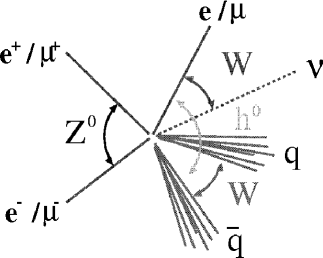
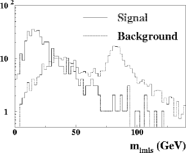
Figure 2.20: $\mathrm{h}^{0}$$\rightarrow$$\mathrm{W}^{+}\mathrm{W}^{-}$: (Left) ${\mathrm{e}}^{+}{\mathrm{e}}^{-}$$\rightarrow$$\mathrm{h}^{0}$$\mathrm{Z}^{0}$$\rightarrow$$\mathrm{W}^{+}\mathrm{W}^{-}$$\ell^{+}\ell^{-}$ topology in leptonic channel ($\mathrm{Z}^{0}$$\rightarrow$${\mathrm{e}}^{+}{\mathrm{e}}^{-}$ or $\mu^{+}\mu^{-}$). (Right) Invariant mass of 3rd lepton and $p_{miss}$ normalized to 10 fb^-1 (about 10 days running at JLC). For signal, plots for 100% decay of the $\mathrm{h}^{0}$$\rightarrow$$\mathrm{W}^{+}\mathrm{W}^{-}$ for 120 GeV Higgs with production cross-section of the SM Higgs.

Note that the recent studies by A. L. C. Sanchez, J. B. Magallanes et al in channel $\mbox{${\mathrm{e}}^{+}{\mathrm{e}}^{-}$}\mbox{$\rightarrow$}\mbox{$\mathrm{Z}^{0}$}\mbox{$\mathrm{h}^{0}$}\mbox{$\rightarrow$}\mbox{$\mathrm{q}\bar{\mathrm{q}}$}WW^{*}\mbox{$\rightarrow$}\mbox{$\mathrm{q}\bar{\mathrm{q}}$}\mbox{$\mathrm{q}\bar{\mathrm{q}}$}\mbox{$\mathrm{q}\bar{\mathrm{q}}$}$, is also on going [34]. The important other channel $\mbox{${\mathrm{e}}^{+}{\mathrm{e}}^{-}$}\mbox{$\rightarrow$}\mbox{$\mathrm{Z}^{0}$}\mbox{$\mathrm{h}^{0}$}\mbox{$\rightarrow$}\nu\bar{\nu}WW^{*}\mbox{$\rightarrow$}\nu\bar{\nu}\mbox{$\mathrm{q}\bar{\mathrm{q}}$}\mbox{$\mathrm{q}\bar{\mathrm{q}}$}$ should also be studied. In this case the 4 jet topology with huge missing mass should be the initial request, and one of the jet-pair invariant mass close to W may be added. An anti-b tagging may also be helpful to suppress the background from $\mathrm{b}\bar{\mathrm{b}}$ decay of the Higgs with multi hard gluon radiation. Also the process, $\mbox{${\mathrm{e}}^{+}{\mathrm{e}}^{-}$}\mbox{$\rightarrow$}\mbox{$\mathrm{Z}^{0}$}\mbox{$\mathrm{h}^{0}$}\mbox{$\rightarrow$}\mbox{$\ell^{+}\ell^{-}$}WW^{*}\mbox{$\rightarrow$}\mbox{$\ell^{+}\ell^{-}$}\mbox{$\mathrm{q}\bar{\mathrm{q}}$}\mbox{$\mathrm{q}\bar{\mathrm{q}}$}$, should be studied.

For the $\mathrm{q}\bar{\mathrm{q}}$ or gluonic decay of the Higgs, the selection were made imposing the $m_{\mathrm{Z}}$ and known Higgs mass. Finally the flavour of the jets assigned to the Higgs are examined and measure the relative branching ratio for the Higgs decay into quarks or gluons. The signature of the gluonic decay is the rather spherical shape of the jets and high multiplicity, while the c-quark decay tends to have sharp jets with much less multiplicity.

In case the Z decays to muons, electrons or quarks, the tau decay is feasible to identify. The tau identification is the key of the measurement. Recoil mass of the leptons or jets originating from the Z also represents the Higgs mass. The direction of the decay products of the taus well represents the direction of the taus. Hence either constraint fits or scaling can be used to have better mass resolution of the invariant mass of the tau-pairs which is to be requested close to Higgs mass. There are many rooms to improve the analyses.

Table 2.3: The simulation results for selection optimized for $\mathrm{h}^{0}$$\rightarrow$$\mathrm{b}\bar{\mathrm{b}}$ at JLC $\sqrt{s}=300$ GeV: Number of events selected for 120 GeV. The SM Higgs cross-section and the branching ratio is used as an input. Event counts are normalized to ${\cal{L}}$=500 fb^-1. Fusion process, which is helpful to increase the signal statistics, is not included in the analysis.

Selection	$\mathrm{q}\bar{\mathrm{q}}$$\mathrm{q}\bar{\mathrm{q}}$	$\nu\bar{\nu}\mbox{$\mathrm{q}\bar{\mathrm{q}}$}$	$\ell^{+}\ell^{-}$$\mathrm{q}\bar{\mathrm{q}}$	Total
$\mathrm{h}^{0}$$\rightarrow$$\mathrm{b}\bar{\mathrm{b}}$	6880	1580	1129	9590
$\mathrm{h}^{0}$$\rightarrow$$\mathrm{c}\bar{\mathrm{c}}$	95	28	15	139
$\mathrm{h}^{0}$$\rightarrow$gg	63	29	12	104
$\mathrm{h}^{0}$$\rightarrow$$\mathrm{W}^{+}\mathrm{W}^{-}$	67	31	18	116
$\mathrm{h}^{0}$$\rightarrow$$\tau^{+}\tau^{-}$	0	0	0	0
non-Higgs SM Bkg	869	374	134	1734

Table 2.4: The simulation results for selection optimized for $\mathrm{h}^{0}$$\rightarrow$$\mathrm{W}^{+}\mathrm{W}^{-}$ at JLC $\sqrt{s}=300$ GeV: Number of events selected for 120 GeV. The SM Higgs cross-section and the branching ratio is used as an input. Event counts are normalized to ${\cal{L}}$=500 fb^-1.

$\mathrm{h}^{0}$$\mathrm{Z}^{0}$$\rightarrow$$\mathrm{W}^{+}\mathrm{W}^{-}$$\mathrm{Z}^{0}$$\rightarrow$	$\ell\nu\mbox{$\mathrm{q}\bar{\mathrm{q}}$}\mbox{$\mathrm{q}\bar{\mathrm{q}}$}$	$\ell\nu\mbox{$\mathrm{q}\bar{\mathrm{q}}$}\mbox{$\ell^{+}\ell^{-}$}$	Total
Efficiency for $\mathrm{h}^{0}$$\mathrm{Z}^{0}$$\rightarrow$$\mathrm{W}^{+}\mathrm{W}^{-}$$\mathrm{q}\bar{\mathrm{q}}$	5.8%	—
Efficiency for $\mathrm{h}^{0}$$\mathrm{Z}^{0}$$\rightarrow$$\mathrm{W}^{+}\mathrm{W}^{-}$$\ell^{+}\ell^{-}$	—	17.3%
Selected Signal	497	142	689
Bkg from other Higgs decay	44	40	84
Bkg from non-Higgs SM	397	77	474
Total Bkg	440	117	557

Results of the preliminary simulation studies

Many studies have been done for varieties of decay channels with simulation with JLC-I model detector, at the typical benchmark points in center-of-mass energies and Higgs masses. Some of the results are summarized in Tab 2.5 and 2.6. Figure 2.21 shows the expected accuracies of the cross-section and branching ratio measurements. The dependence of the center-of-mass energy on the sensitivity of the branching ratio and Yukawa-coupling are shown in figures 2.22 and 2.23, respectively. Note that we neglect the huge signal contribution especially at higher energy from the WW-fusion process. Hence the signal events used in these analyses are considerably less at higher energies (400 and 500 GeV) than 300 GeV, which leads the worse sensitivity at higher energies. When we include the WW-fusion process, the sensitivity is expected to be similar at 300–500 GeV. Table 2.7 summarizes the accuracies of the measurements obtained in these studies so far for $\sqrt{s}=$300, 400 and 500 GeV, for a Higgs boson mass of 120 GeV, with $\cal{L}=$500 fb^-1.

Table 2.5: Accuracy in the branching ratio obtained in the analysis for ${\cal{L}}$=500 fb^-1, and for 120 GeV Higgs. Note that the WW-fusion process, which increases the signal statistics significantly at higher energy, is not used in the analysis so far.

$\sqrt{s}$	300 GeV	400 GeV	500 GeV
$\Delta$Br/Br
$\mathrm{h}^{0}$$\rightarrow$$\mathrm{b}\bar{\mathrm{b}}$	1.1%	1.3%	1.7%
$\mathrm{h}^{0}$$\rightarrow$$\mathrm{W}^{+}\mathrm{W}^{-}$	5.1%	12%	16%
$\mathrm{h}^{0}$$\rightarrow$$\tau^{+}\tau^{-}$	4.4%	—	—
$\mathrm{h}^{0}$$\rightarrow$$\mathrm{c}\bar{\mathrm{c}}$+gg	6.3%	—	—
$\mathrm{h}^{0}$$\rightarrow$$\mathrm{c}\bar{\mathrm{c}}$	22%	23%	27%
$\mathrm{h}^{0}$$\rightarrow$gg	10%	11%	13%
$\mbox{$\mathrm{h}^{0}$}\mbox{$\rightarrow$}\gamma\gamma$	—	—	—
$\mbox{$\mathrm{h}^{0}$}\mbox{$\rightarrow$}\mbox{$\mathrm{Z}^{0}$}\gamma$	—	—	—

Table 2.6: Accuracy in the branching ratio obtained in the analysis for ${\cal{L}}$=500 fb^-1, and for 140 GeV Higgs. Note that the WW-fusion process, which increases the signal statistics significantly at higher energy, is not used in the analysis so far.

$\sqrt{s}$	300 GeV	400 GeV	500 GeV
$\Delta$Br/Br
$\mathrm{h}^{0}$$\rightarrow$$\mathrm{b}\bar{\mathrm{b}}$	2.1%	2.3%	2.6%
$\mathrm{h}^{0}$$\rightarrow$$\mathrm{W}^{+}\mathrm{W}^{-}$	2.0%	3.3%	4.5%

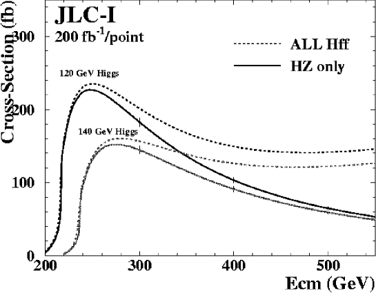
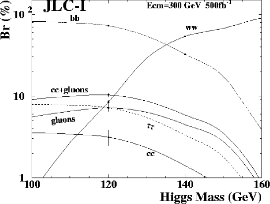
Figure 2.21: (Top) Production cross-section (for M_H=120 and 140 GeV) as a function of $\sqrt{s}$. The accuracy in the cross-section measurement in $\mathrm{h}^{0}$$\mathrm{Z}^{0}$ process are shown at 300, 400 and 500 GeV as error bars, assuming 200 fb^-1 at each $\sqrt{s}$ point. (Bottom) Branching ratio of the SM Higgs as a function of the Higgs mass. The measurements errors obtained in the simulation studies done so far are also shown in error bars. Note that the theoretical errors are not shown in this plot.

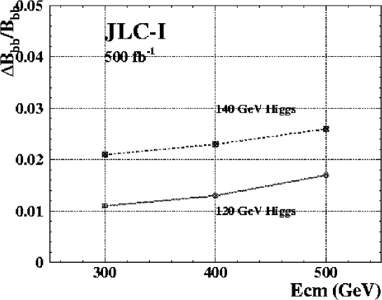
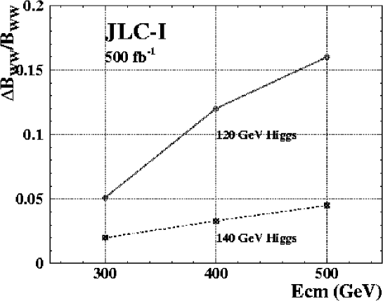
Figure 2.22: Expected measurement error $\Delta$Br/Br in Br($\mathrm{h}^{0}$$\rightarrow$$\mathrm{b}\bar{\mathrm{b}}$) and Br($\mathrm{h}^{0}$$\rightarrow$$\mathrm{W}^{+}\mathrm{W}^{-}$), for 120 and 140 GeV SM Higgs as a function of $\sqrt{s}$. Luminosity of 500 fb^-1 ($\sim$3 years JLC-I running) is used: Note that the huge contribution from the WW-fusion especially at the high energy is neglected in this analysis. Including the process, the sensitivity at 500 GeV is expected to be similar to that of 300 GeV.

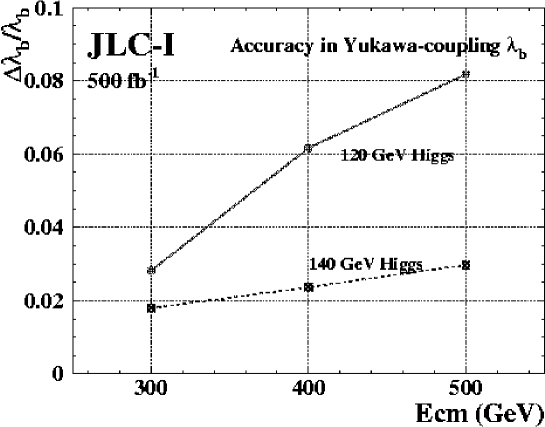
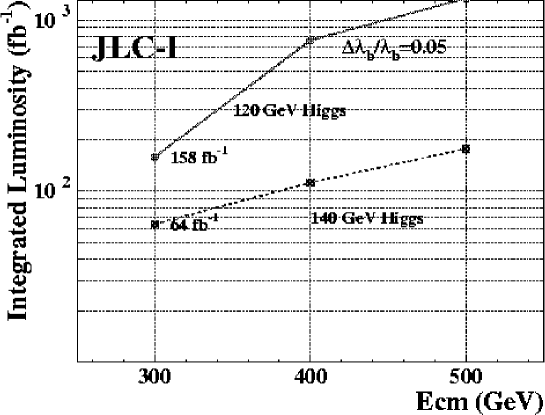
Figure 2.23: (Top) expected measurement error in Yukawa-coupling to b-quark, $\Delta\lambda_{b}/\lambda_{b}$, for 120 and 140 GeV SM Higgs as a function of $\sqrt{s}$. Luminosity of 500 fb^-1 ($\sim$3 years JLC running) is used: (Bottom) necessary luminosity for measurement of $\lambda_{b}$ to achieve 5% error which is similar to current knowledge of the b-quark mass. The luminosity of less than 160 fb^-1 is necessary to achieve the 5% accuracy for 120–140 GeV Higgs. Note that the huge contribution from the WW-fusion especially at the high energy is neglected in this analysis. Including the process, the sensitivity at 500 GeV is expected to be similar to that of 300 GeV.

Table 2.7: Accuracy at $\sqrt{s}=$300, 400 and 500 GeV with ${\cal{L}}$=500 fb^-1 for 120 GeV CP-even Higgs at JLC. The Higgs boson of SM-like is used as an input.

$\sqrt{s}$	300 GeV	400 GeV	500 GeV
$\Delta\mbox{$m_{\mathrm{h}}$}$ (lepton-only)	80 MeV	—	—
$\Delta\mbox{$m_{\mathrm{h}}$}$	40 MeV	—	—
$\Delta\sigma/\sigma$ (lepton-only)	2.1%	2.5%	2.9%
$\Delta\sigma/\sigma$	1.3%	—	—
$\Delta(\sigma_{h\nu\bar{\nu}}\cdot$Br($\mathrm{b}\bar{\mathrm{b}}$)	2.0%	—	—
ZZH-coupling $\Delta$ZZH/ZZH	1.1%	1.3%	1.5%
WWH-coupling $\Delta$WWH/WWH	1.6%	—	—
$\Delta\Gamma_{\mbox{$\mathrm{h}^{0}$}}/\Gamma_{\mbox{$\mathrm{h}^{0}$}}$	5.5%	12%	16%
Yukawa coupling $\Delta\lambda/\lambda$
$\lambda_{b}$	2.8%	6.1%	8.1%
$\lambda_{\tau}$	3.5%	—	—
$\lambda_{c}$	11.3%	13%	15%
$\lambda_{b}/\lambda_{\tau}$	2.3%	—	—
$\lambda_{b}/\lambda_{c}$	11%	12%	14%
$\lambda_{up-type}$	4.1%	—	—
$\lambda_{down-type}/\lambda_{up-type}$	3.2%	—	—
$\Delta(\sigma\cdot$Br)/$(\sigma\cdot$Br)
$\mathrm{h}^{0}$$\rightarrow$$\mathrm{b}\bar{\mathrm{b}}$	1.1%	1.3%	1.7%
$\mathrm{h}^{0}$$\rightarrow$$\mathrm{W}^{+}\mathrm{W}^{-}$	5.1%	12%	16%
$\mathrm{h}^{0}$$\rightarrow$$\tau^{+}\tau^{-}$	4.4%	—	—
$\mathrm{h}^{0}$$\rightarrow$$\mathrm{c}\bar{\mathrm{c}}$+gg	6.3%	—	—
$\mathrm{h}^{0}$$\rightarrow$$\mathrm{c}\bar{\mathrm{c}}$	22%	23%	27%
$\mathrm{h}^{0}$$\rightarrow$gg	10%	11%	13%
$\mbox{$\mathrm{h}^{0}$}\mbox{$\rightarrow$}\gamma\gamma$	—	—	—
$\mbox{$\mathrm{h}^{0}$}\mbox{$\rightarrow$}\mbox{$\mathrm{Z}^{0}$}\gamma$	—	—	—

2.6 Physics Outputs and Impacts in Models

In this section, we discuss impacts of the Higgs boson studies at JLC. Using the production cross section and the branching ratios of the Higgs boson, we show how and to what extent the SM is distinguished from other models like two Higgs doublet model and MSSM. Within the context of the MSSM, we can determine the parameters of the model, especially the heavy Higgs boson mass from the properties of the lightest Higgs boson. We also discuss the implications of the Higgs study when the heavy Higgs bosons or SUSY particles are discovered at LHC and JLC experiments.

2.6.1 Model-independent Analysis for the Higgs Boson Couplings

In order to distinguish various models, we first introduce a model-independent parameterization for various couplings to Higgs boson. The following four parameters represent the multiplicative factors in the Higgs-boson coupling constants with down-type quarks, up-type quarks, charged-leptons and gauge bosons.

$$L = x\frac{m_{b}}{v}h\bar{b}b+y(\frac{m_{t}}{v}h\bar{t}t+\frac{m_{c}}{v}h\bar{c}c)$$ (2.9)

$$+z\frac{m_{\tau}}{v}h\bar{\tau}\tau+u(gm_{W}hW_{\mu}W^{\mu}+\frac{\sqrt{g^{2}+g^{\prime 2}}}{2}m_{Z}hZ_{\mu}Z^{\mu}),$$

where the coupling with light quarks and leptons are suppressed. This is, of course, not general way to parameterize the coupling constants. We can introduce different parameters for charm and top quarks, and $W$ and $Z$ bosons, and flavour-changing couplings are also possible. The above parameterization is still useful because models such as MSSM, NMSSM and multi-Higgs doublet model without tree-level flavour changing neutral current fall into this category.

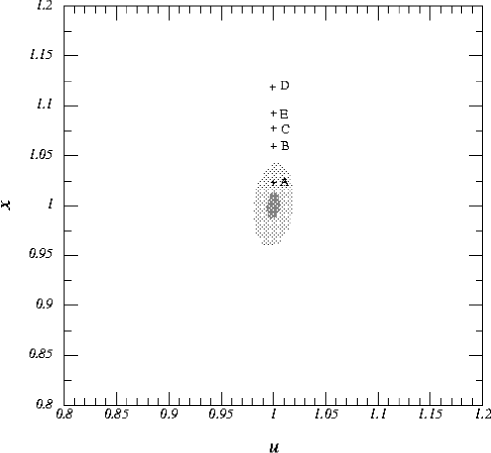
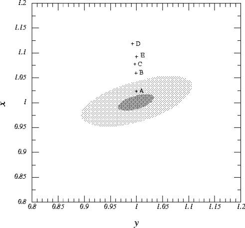
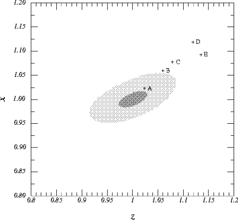
Figure 2.24: Experimental statistical accuracy of the parameter determination in $u-x$, $y-x$, and $z-x$ space at the JLC experiment with an integrated luminosity of 500 fb^-1 and $\sqrt{s}=300$ GeV. The inner (outer) contour is the 1 $\sigma$ (95% CL) curve. The input point is the SM point $(x=y=z=u=1)$. The Higgs boson mass is 120 GeV. The points A - E correspond to the projections on each plane of the $x,y,z,$ and $u$ values evaluated in the following parameter sets of the MSSM. ($m_{A}$ (GeV), $M_{S}$ (GeV), $X_{t}$, $\tan{\beta}$) are (1000, 500, 0, 10), (600, 550, -2, 10), (550, 1430, 2, 5), (450, 25430, 0, 4) and (500, 4810, 2, 30) for A - E, respectively. We also take the gluino mass $(M_{3})$ and the higgsino mass parameter $(\mu)$ as 300 GeV.

In Figure 2.24, we show the expected accuracy of the parameter determination in four dimensional space at the JLC experiment with an integrated luminosity of 500 fb^-1. We use the production cross section and branching ratios listed in Table 2.5 for the case of $\sqrt{s}=300$ GeV and $m_{h}=$ 120 GeV. The input point is taken to be the SM point. We can see that the $u$ and $x$ parameters are determined to a few % level, and $y$ and $z$ are constrained to less than 10 %. $x$, $y$, $z$, and $u$ in various models are given by model parameters as listed in Table 2.8. In the MSSM model, in addition to the tree level coupling constants, we take into account the correction to the $hb\bar{b}$ coupling constant denoted by $\epsilon_{b}$ defined in section 2.1, whose effect becomes significant only for large values of $\tan{\beta}$. We also assume that the coupling of the Higgs boson with two gluons is dominated by the internal top-quark loop diagram, although the SUSY loop corrections become sizable in some parameter space. In the figure we also show points corresponding to several input parameters in the MSSM. From the correlation of the four parameters determined at the LC experiment, it is possible to distinguish various models. For example, Type-I Higgs doublet model and MSSM have different relation in the $x-y$ space. For a large $\tan{\beta}$ value, the allowed range of the $x-z$ plane can deviate from the $x=z$ line for the MSSM because of the SUSY correction to the $hb\bar{b}$ vertex, as shown for the point E.

Table 2.8: The parameters $x$, $y$, $z$, and $u$ in various models. Two choices of the parameters are shown for the Type I two Higgs doublet model.

model	$x$	$y$	$z$	$u$
SM	1	1	1	1
Type-I Two Higgs doublet Model	$-\frac{\sin{\alpha}}{\cos{\beta}}$($\frac{\cos{\alpha}}{\sin{\beta}}$)	$-\frac{\sin{\alpha}}{\cos{\beta}}$($\frac{\cos{\alpha}}{\sin{\beta}}$)	$-\frac{\sin{\alpha}}{\cos{\beta}}$($\frac{\cos{\alpha}}{\sin{\beta}}$)	$\sin{(\beta-\alpha)}$
Type-II Two Higgs doublet Model	$-\frac{\sin{\alpha}}{\cos{\beta}}$	$\frac{\cos{\alpha}}{\sin{\beta}}$	$-\frac{\sin{\alpha}}{\cos{\beta}}$	$\sin{(\beta-\alpha)}$
MSSM	$-\frac{\sin{\alpha}}{\cos{\beta}}\frac{1-\epsilon_{b}/\tan{\alpha}}{1+\epsilon_{b}\tan{\beta}}$	$\frac{\cos{\alpha}}{\sin{\beta}}$	$-\frac{\sin{\alpha}}{\cos{\beta}}$	$\sin{(\beta-\alpha)}$

2.6.2 Determination of Heavy Higgs Boson Mass in MSSM

As we discuss in section 2.5.5 we can put constrains on the CP-even Higgs boson mass ($m_{A}$) from the branching ratios of the lightest CP even Higgs boson in the MSSM. Within the approximation that the stop mixing is neglected in the one-loop Higgs potential and the $hb\bar{b}$ vertex correction is small, we can derive the following formulas for $y^{2}/x^{2}$, $y^{2}/z^{2}$, $u^{2}/x^{2}$, and $u^{2}/z^{2}$, which corresponds to $(B(h\rightarrow c\bar{c})+B(h\rightarrow gg))/B(h\rightarrow b\bar{b})$, $(B(h\rightarrow c\bar{c})+B(h\rightarrow gg))/B(h\rightarrow\tau^{+}\tau^{-})$, $B(h\rightarrow W^{(*)}W^{(*)})/B(h\rightarrow b\bar{b})$, and $B(h\rightarrow W^{(*)}W^{(*)})/B(h\rightarrow\tau^{+}\tau^{-})$, respectively.

$$y^{2}/x^{2} = y^{2}/z^{2}=\left(\frac{m_{A}^{2}-m_{h}^{2}}{m_{A}^{2}+m_{Z}^{2}}\right)^{2}\left(1-\frac{m_{h}^{2}-m_{Z}^{2}}{m_{A}^{2}-m_{h}^{2}}\frac{1}{\tan^{2}{\beta}}\right)^{2},$$ (2.10)

$$u^{2}/x^{2} = u^{2}/z^{2}=\left(\frac{m_{A}^{2}-m_{h}^{2}}{m_{A}^{2}+m_{Z}^{2}}\right)^{2}\left(1+\frac{2m_{Z}^{2}}{m_{A}^{2}-m_{h}^{2}}\frac{1}{1+\tan^{2}{\beta}}\right)^{2}.$$ (2.11)

For $m_{A}\hbox{ \raise 3.0pt\hbox to0.0pt{$>$}\raise-3.0pt\hbox{$\sim$} }200$ GeV, the first equation shows that $y^{2}/x^{2}$ and $y^{2}/z^{2}$ are approximately given by $(m_{A}^{2}-m_{h}^{2})^{2}/(m_{A}^{2}+m_{Z}^{2})^{2}$ because of the small factor of $(m_{h}^{2}-m_{Z}^{2})/(m_{A}^{2}-m_{h}^{2})$. From the second equation, we see that $u^{2}/x^{2}$ and $u^{2}/z^{2}$ are also given by the same quantity if $\tan{\beta}$ is not small. This should be a good approximation because the Higgs boson search at LEP already excluded the region of $\tan{\beta}\hbox{ \raise 3.0pt\hbox to0.0pt{$<$}\raise-3.0pt\hbox{$\sim$} }2$. If we take into account the stop mixing effects in the one-loop Higgs potential and the $hb\bar{b}$ vertex correction denoted by $\epsilon_{b}$, the above approximate formulas receive corrections.

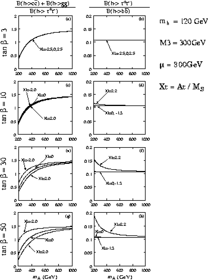
Figure 2.25: $(B(h\rightarrow c\bar{c})+B(h\rightarrow gg))/B(h\rightarrow\tau^{+}\tau^{-})$ and $B(h\rightarrow\tau^{+}\tau^{-})/B(h\rightarrow b\bar{b})$ of the 120GeV lightest CP-even Higgs boson for $\tan\beta=3,10,30,$ and $50$.

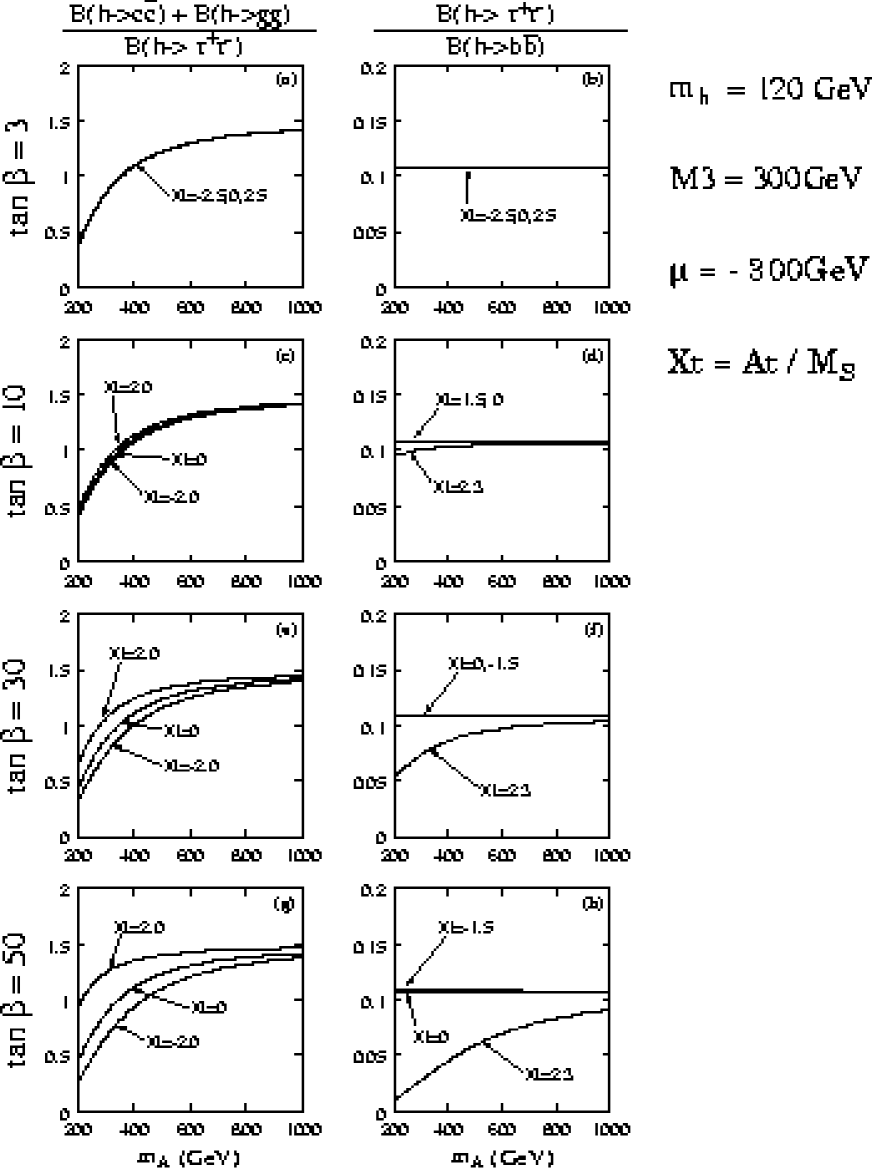
Figure 2.26: The same as Figure 2.26, except $\mu=-300$ GeV.

In order to show numerical impacts of these corrections we present $(B(h\rightarrow c\bar{c})+B(h\rightarrow gg))/B(h\rightarrow\tau^{+}\tau^{-})$ and $B(h\rightarrow\tau^{+}\tau^{-})/B(h\rightarrow b\bar{b})$ for different choices of $\tan{\beta}$ in Figure 2.25 (Figure 2.26). Here we introduce a SUSY breaking scale $M_{S}$ as $m^{2}_{\tilde{q_{3}}_{L}}=m^{2}_{\tilde{t}_{R}}=m^{2}_{\tilde{b}_{R}}=M_{S}^{2}$ and the squark mixing parameter $A_{t}=X_{t}M_{S}$ and $A_{b}=0$. We set the gluino mass $(M_{3})$ as 300 GeV and the higgsino mass parameter $(\mu)$ as 300 GeV (-300 GeV) and fix the Higgs boson mass as 120 GeV and solve $M_{S}$ in term of $\tan{\beta}$, $X_{t}$ and $m_{A}$. The possible range of the ratios are shown as a function of $m_{A}$ by changing the parameter $X_{t}$. Notice that $B(h\rightarrow\tau^{+}\tau^{-})/B(h\rightarrow b\bar{b})$ is the same as the SM prediction and therefore independent of $m_{A}$ if $\epsilon_{b}$ vanishes. In Figure 2.25 and Figure 2.26, the plots (b) and (d) show that the effect of $\epsilon_{b}$ on this ratio is tiny for $\tan\beta\hbox{ \raise 3.0pt\hbox to0.0pt{$<$}\raise-3.0pt\hbox{$\sim$} }10$. On the other hand, for large $\tan\beta$, e.g. the plot (h), the deviation of this ratio from the SM value can be significant. Furthermore, by comparing Figure 2.25(h) and Fig 2.26(h), we can see that the effect of $\epsilon_{b}$ enhances or suppresses the ratio depending on the sign of $\mu$. In the plots (e) and (g) of Figure 2.25 and Figure 2.26, we can see that the deviation of $y^{2}/z^{2}$ from the above approximate formula is large for $\tan{\beta}\hbox{ \raise 3.0pt\hbox to0.0pt{$>$}\raise-3.0pt\hbox{$\sim$} }30$. Since $y$ and $z$ are independent of $\epsilon_{b}$, this deviation is due to the stop mixing effects on the one-loop Higgs potential. On the other hand, the correction is small for $\tan{\beta}\hbox{ \raise 3.0pt\hbox to0.0pt{$<$}\raise-3.0pt\hbox{$\sim$} }10$. Because it is likely that the only one light Higgs boson is found in the LHC experiment for $3\hbox{ \raise 3.0pt\hbox to0.0pt{$<$}\raise-3.0pt\hbox{$\sim$} }tan{\beta}\hbox{ \raise 3.0pt\hbox to0.0pt{$<$}\raise-3.0pt\hbox{$\sim$} }10$, the indirect determination on $m_{A}$ could become very important in such parameter space. Note, however, that the deviation from the approximate formula depends on the magnitude of $\mu$. For larger $|\mu|$ the deviation can be significant even for $\tan\beta\hbox{ \raise 3.0pt\hbox to0.0pt{$<$}\raise-3.0pt\hbox{$\sim$} }10$.

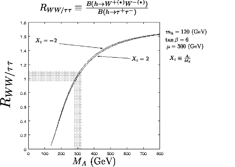
Figure 2.27: The ratio $B(h\rightarrow W^{+(*)}W^{-(*)})/B(h\rightarrow\tau^{+}\tau^{-})$ of the 120 GeV lightest Higgs boson for $\tan\beta=6$, $\mu=300$ GeV, and $X_{t}=\pm 2$ as a function of $m_{A}$. The shaded area shows the $m_{A}$ determination from the ratio, obtained by the assumption that $B(h\rightarrow W^{+(*)}W^{-(*)})/B(h\rightarrow\tau^{+}\tau^{-})$ is determined in 6.7% accuracy (see Table2.9).

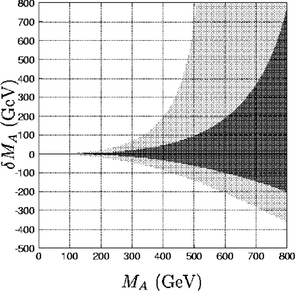
Figure 2.28: Accuracy of the $m_{A}$ determination as a function of $m_{A}$ from branching ratio measurements. The dark area corresponds to the error of $m_{A}$ from $B(h\rightarrow c\bar{c})+B(h\rightarrow gg)$, $B(h\rightarrow\tau^{+}\tau^{-})$, and $B(h\rightarrow W^{(*)}W^{(*)})$ measurements at the JLC experiment. The light area is obtained by the assumption that $\Gamma(h\rightarrow W^{(*)}W^{(*)})/\Gamma(h\rightarrow\tau^{+}\tau^{-})$ is determined in 15% accuracy, which corresponds to an estimated statistical error at the LHC experiment.

Table 2.9: The errors of the double ratios for the 120 GeV SM Higgs boson due to the theoretical uncertainties of input parameters and experimental statistical errors (%) for JLC with an integrated luminosity of 500 fb^-1 and $\sqrt{s}$ = 300 GeV. For theoretical errors, we take into account the uncertainty from the strong coupling constant and the bottom and charm quark masses as ${\alpha}_{s}(m_{Z})=0.1181\pm 0.002,{m}^{\overline{MS}}_{b}(m_{b})=4.20\pm 0.13~{}\mbox{GeV}~{}(\pm 3\%),{m}^{\overline{MS}}_{c}(m_{c})=1.25\pm 0.06~{}\mbox{GeV}~{}(\pm 5\%).$

	Theoretical error	Experimental error	Total error
$\frac{Br(h\rightarrow c\bar{c})+Br(h\rightarrow gg)}{Br(h\rightarrow b\bar{b})}$	8.6	6.4	10.7
$\frac{Br(h\rightarrow W^{(*)}W^{(*)})}{Br(h\rightarrow b\bar{b})}$	7.6	5.2	9.2
$\frac{Br(h\rightarrow c\bar{c})+Br(h\rightarrow gg)}{Br(h\rightarrow\tau^{+}\tau^{-})}$	4.1	7.7	8.7
$\frac{Br(h\rightarrow W^{(*)}W^{(*)})}{Br(h\rightarrow\tau^{+}\tau^{-})}$	0	6.7	6.7

The ratio of the branching ratios is useful to constrain $m_{A}$ as shown in Figure 2.27. In Figure 2.28, we show the precision of the indirect determination on $m_{A}$ from the above branching ratios at the JLC experiment with integrated luminosity of 500 fb^-1 at $\sqrt{s}=300$ GeV. The Higgs boson mass is taken to be 120 GeV. The theoretical uncertainty of the branching ratio calculation in the SM and the estimated experimental statistical errors are summarized in Table 2.9. The combined error to determine $m_{A}$ from $(B(h\rightarrow c\bar{c})+B(h\rightarrow gg))/B(h\rightarrow b\bar{b})$ and $B(h\rightarrow W^{(*)}W^{(*)})/B(h\rightarrow b\bar{b})$ is 7.0 %, and that from $(Br(h\rightarrow c\bar{c})+Br(h\rightarrow gg))/Br(h\rightarrow\tau^{+}\tau^{-})$ and $Br(h\rightarrow W^{(*)}W^{(*)})/Br(h\rightarrow\tau^{+}\tau^{-})$ is 5.3%. In order to draw the upper and lower limits of $m_{A}$, we use the 5.3% error and assume that these ratios normalized by the SM values are given by $(m_{A}^{2}-m_{h}^{2})^{2}/(m_{A}^{2}+m_{Z}^{2})^{2}$. Notice that for the ratios normalized by $Br(h\rightarrow\tau^{+}\tau^{-})$, there is no correction from the $\epsilon_{b}$ term. We can see that the useful upper bound of the heavy Higgs boson mass is obtained, if the true value of $m_{A}$ is less than 600 GeV. Even if the branching ratio is consistent to the SM value, the lower bound will be determined. This is compared with the precision of the ratio of partial decay widths $\Gamma(h\rightarrow W^{(*)}W^{(*)})/\Gamma(h\rightarrow\tau^{+}\tau^{-})$ at LHC. Using the weak boson fusion process for Higgs boson production, the statistical error is estimated to be 15% for the integrated luminosity of 200 fb^-1[35].

When $tan{\beta}$ is large, we may be able to determine the parameter $\Delta_{b}\equiv\epsilon_{b}\tan{\beta}$ from production cross section and branching ratios. As an example we show the experimental statistical accuracy of the MSSM parameter determination including $\Delta_{b}$. We present the $\chi^{2}$ contour in $1/(\tan{\alpha}\tan{\beta})$, $\sin{(\beta-\alpha)}$, and $\Delta_{b}$ space for $\tan{\beta}=10$ (Figure 2.29) and $\tan{\beta}=50$ (Figure 2.30). We can see that non-zero $\Delta_{b}$ can be clearly distinguished in the case of $\tan{\beta}=50$. Establishing the non-vanishing $\Delta_{b}$ is very interesting because it is induced by virtual correction due to SUSY particles.

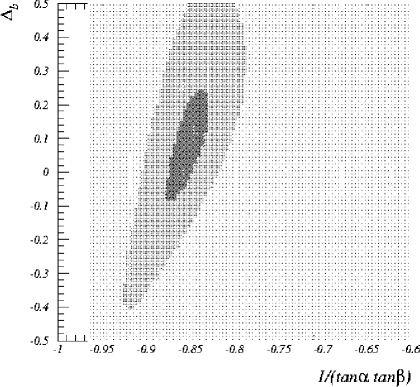
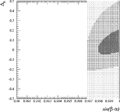
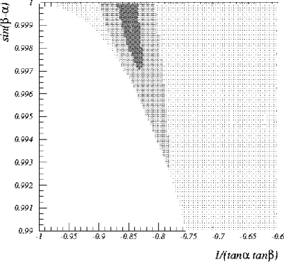
Figure 2.29: Experimental statistical accuracy of the $1/(\tan{\alpha}\tan{\beta})$, $\sin{(\beta-\alpha)}$, and $\Delta_{b}$ determination for $\tan{\beta}=10$ in the MSSM. The darkest (second darkest) area corresponds to the 1$\sigma$ (95% CL) region. No solution is obtained in the white area. The input point is $1/(\tan{\alpha}\tan{\beta})=-0.852$, $\sin{(\beta-\alpha)}=0.99985$, and $\Delta_{b}(\equiv\epsilon_{b}\tan{\beta})=0.08$, corresponding to SUSY parameters, $m_{A}$=400 GeV, $M_{S}$=654 GeV, $X_{t}$=2, $\mu$ =300 GeV, and $M_{3}$ = 300 GeV.

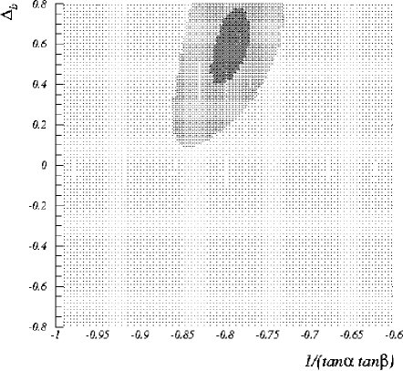
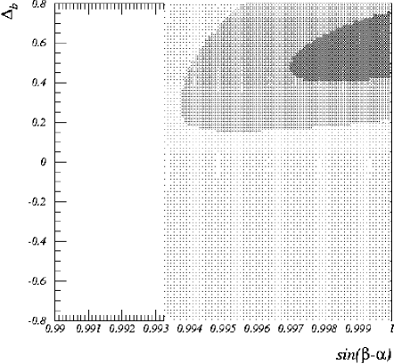
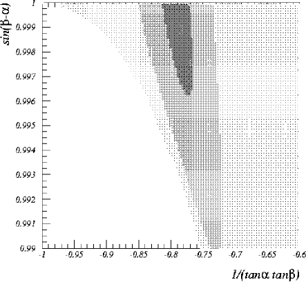
Figure 2.30: The same figure as Figure 2.29 for the case of $\tan{\beta}=50$. The input point is $1/(\tan{\alpha}\tan{\beta})=-0.793$, $\sin{(\beta-\alpha)}=0.999986$, and $\Delta_{b}(\equiv\epsilon_{b}\tan{\beta})=0.58$, corresponding to SUSY parameters, $m_{A}$=400 GeV, $M_{S}$=462 GeV, $X_{t}$=2, $\mu$ =300 GeV and $M_{3}$ = 300 GeV.

2.6.3 Possible Scenarios of SUSY Parameter Determination

If the heavy Higgs bosons or SUSY particles are found in the LHC experiment and the JLC experiment, we can perform many consistency checks, coupling constant determinations, and model discrimination with help of the Higgs boson studies. Possible scenarios are as follows:

• If the heavy Higgs bosons $(A$ and $H)$ are found, we can compare their masses with the value determined from branching measurement of the lightest Higgs boson. This is an important test of the MSSM because two values are not necessarily the same for two Higgs doublet model in general.

• If the stop sectors are determined from the direct SUSY search in addition to the information on $m_{A}$ from either direct discovery of the heavy Higgs bosons or indirect determination from the branching measurements, we can determine $\tan{\beta}$ from the mass formula of the lightest CP-even Higgs boson in the MSSM. In order to do so, it is important to determine two masses and the left-right mixing of the stop sector, because the mixing parameter gives a sizable correction to the lightest Higgs boson mass.

• If $\tan{\beta}$ value is obtained from other sectors of the SUSY model, we can compare it with $\tan{\beta}$ inferred from the studies on the lightest Higgs boson. For possibilities of other $\tan{\beta}$ measurements, we can consider the stau decay[36], the heavy Higgs production and decay[37], and the chargino and neutralino production[38]. The consistency of $\tan{\beta}$ determination is in fact the direct confirmation of the MSSM Higgs mass formula, and tells us that the Lagrangian of the Higgs sector is likely to be that of the MSSM. If there is a deviation we have to extend the Higgs sector. For example, we may be able to give a constraint on the additional coupling constant in the mass formulas of the NMSSM Higgs sector, which is given by

  $$m_{h}^{2}\leq\frac{1}{2}\lambda^{2}v^{2}\sin^{2}{2\beta}+m_{Z}^{2}\cos^{2}{2\beta}+\frac{3}{2\pi^{2}}\frac{m_{t}^{4}}{v^{2}}ln{\frac{m_{stop}^{2}}{{m_{t}}^{2}}},$$ (2.12)

  where $\lambda$ is a new coupling constant associated with a singlet Higgs field. It is conceivable that the upper bound is saturated for the lightest CP-even Higgs boson and therefore its properties are not much different from the SM Higgs boson. From precise determination of the Higgs boson properties, the stop sector, and $\tan{\beta}$ from other processes, we may be able to distinguish NMSSM from MSSM and determine the parameter $\lambda$.

In this way, studies of the Higgs boson properties are useful to determine the Lagrangian of the SUSY model. Through the Higgs mass formula, we can obtain information on various SUSY parameters. The precision studies of the Higgs boson, therefore, play an important role in distinguishing and establishing different models, even after the discovery of SUSY particles.

2.7 Further Experimental Considerations

In studies of the Higgs particles at JLC, accurate tracking and event kinematic reconstructions are essential. One needs to investigate the performances of such key techniques under very realistic experimental environments. The extremely high luminosity of order of $10^{34}$ cm^-2s^-1, which is about 2 order higher than that at LEP, and the beam structure necessary for the acceleration in the linear collider JLC, make the experimental situation more severe than that at LEP and SLC in the following points;

• Large number of noise hits on the vertex detectors due to huge number of ${\mathrm{e}}^{+}{\mathrm{e}}^{-}$ pairs created by beam-beam interactions [21]. It makes proper associations of the hits for the tracking difficult especially for the low momentum tracks, which are rather important for ${\rm b}$ tagging, due to multiple Coulomb scatterings and energy losses in detector materials;

• Overlap of two or more physics events, especially two-photon backgrounds [33], in a same bunch collision with a signal or other hard scattering event due to very high integrated luminosity per bunch. It might reach to 1 $\mu$b^-1 level at JLC which is 2–3 order higher than that at LEP/SLC. The average rate of the overlap of the two photon process on signal events might reach to about 10 % or more

• Degradation of the collision energy due to beamstrahlung.

The studies have been made with the current design of the detector at JLC [17] as a model detector.

Studies of the Higgs measurements with such expected experimental condition have been attempted [22]. The most inner layer of the vertex detector might have the noise hit density of about 1 hits/mm², which makes proper associations of the hits difficult especially for the low momentum tracks. For the event overlapping, there are two major effects in the measurements. One is the effect on the kinematics such as reconstructed mass of the Higgs and the selection bias. The other effect is on the flavour tagging which relies on the tracks displaced from the event primary vertex.

2.7.1 Noise Hits on Vertex Detector due to Beam-beam Interaction

The beam at JLC has 50–100 of bunches in a beam train with bunch spacing of 1.4 to 5.6 nsec and the repetition rate of 50–150 Hz. Since the present design uses CCD readout for the vertex detector, the hits from multi-bunches in a train overlap each other. In single train collision, the expected rate of the noise hits due to the beam-beam interaction is about 30–100 hits/cm² on the inner most layer of the vertex detectors. Studies have been made with full simulation program JIM [19] based on the GEANT3 package. Tracking devices in the JLC detector are: central tracker (CT), intermediate tracker (IT) and vertex detector (VX). Detector parameters are summarized in Tab 2.10.

Table 2.10: Detector parameters which are relevant to this analysis. Magnetic field of 2 T is used.

Detector	No. of	Radius of layers [cm]		Half-$z$	Resolution [$\mu{\rm m}$]
Name	Layers	Inner	Outer	Length [cm]	$r$-$\phi$	$z$
CT	100	45	230	125	100	2000
IT	5	10	38	21-79	20	20
VX	4	2.4	6.0	5-12.5	4	4

Single $\mu$ track generated with flat distribution in polar angle in cos$\theta\pm$0.8 with momentum ranging from 0.5 to 50 GeV, are used as a “signal” track to study the proper track finding efficiency. Two kinds of backgrounds are considered in this analysis. One is the low energy $\mbox{${\rm e}$}^{+}\mbox{${\rm e}$}^{-}$ pairs induced by the beam-beam interactions. This background is simulated by the CAIN code [39], and generated $\mbox{${\rm e}$}^{+}\mbox{${\rm e}$}^{-}$ pairs are also processed through the same full detector simulation program. The simulated detector response from the $\mbox{${\rm e}$}^{+}\mbox{${\rm e}$}^{-}$ pairs, corresponding to numbers of bunch collisions (100 bunches as a default), are overlapped to each signal event. Another background source added are low momentum charged tracks from two-photon process (corresponding to 10 events as a default).

First step of the analysis starts from the reduction of the noise hits with cluster shape analyses. Almost all the background hits in the VX detector are generated by very low momenta $\mbox{${\rm e}$}^{+}\mbox{${\rm e}$}^{-}$’s which are curling as a helix with small radius within the VX detector region. Thus the shape of the cluster of the noise hits on the VX tends to be longer than that of hits generated by “signal” charged tracks. By applying cuts on shapes of VX hit cluster, number of background hits has been reduced to 1/3 keeping the signal hit efficiency to be more than 98 %.

We start the tracking from the fitting of the hits in the CT. Then the hits in IT are associated to these tracks. Since most of the problematic $\mbox{${\rm e}$}^{+}\mbox{${\rm e}$}^{-}$pairs have very low momenta, the hit density in IT region is already low enough. Hence the association of the hits on the IT is rather easy. Then analysis proceeds to the association of the tracks obtained from CT and IT (CT+IT track) to the clusters found in the VX. We have compared the following two methods for the association;

1. a conventional “Road Method”: The positions predicted by the CT+IT track are compared with those of VX clusters in each VX layer, and nearest clusters are retained.

2. “Local Tracking”: first, candidates of track segments are locally made only with the VX clusters. In order to reduce the combinatorial associations, accumulated distribution of VX hits in all layers in the $\phi$-$z$ plane is used, and peaked clusters in the plane are defined as a local track segments. Then the track parameters of the local segments are compared with those of CT+IT tracks, and associated to the most appropriate tracks from the CT+IT. Finally re-fits are made globally for all hits found in CT, IT and VX.

To check the tracking performance, we define the proper tracking as the track having correct hit association for all layers of VX. Dependence of the proper tracking efficiency on the momentum of the signal $\mu$ is shown in Fig 2.31. As a default, the $\mbox{${\rm e}$}^{+}\mbox{${\rm e}$}^{-}$ pairs from 100 bunch-interactions and charged tracks from 10 two-photon events are overlapped. Especially for charged tracks with momentum below 1 GeV, difference of efficiencies between two methods mentioned above are fairly large. Fig2.32 shows the proper track reconstruction efficiencies as functions of the amount of overlapped background of; (upper) $\mbox{${\rm e}$}^{+}\mbox{${\rm e}$}^{-}$ pairs indicated by the number of bunches in a train, and (lower) two-photon processes. The signal $\mu$ momentum is fixed to 1 GeV. For both cases, amount of the other background is fixed to the default values.

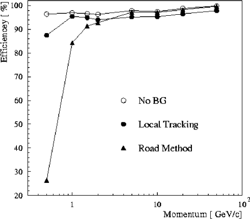
Figure 2.31: Momentum dependence of proper track reconstruction efficiency.

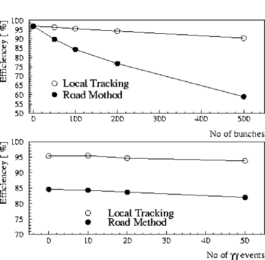
Figure 2.32: Noise hit rate dependence of track reconstruction efficiency for 1 GeV single muon.

Efficiencies obtained by two track finding methods do not depend on amount of overlapped two-photon background significantly. The degradation of the efficiency obtained by the “Local Tracking” method is found to be small even at the extremely high background rate, while the efficiency by the simple “Road method” decreases rapidly as amount of background from $\mbox{${\rm e}$}^{+}\mbox{${\rm e}$}^{-}$ pairs grows. In order to perform a good tracking, a self-fit capability in vertex detector is found to be very helpful. Parameters in this method should be optimized further. Also an interpolation of tracks taking into account energy losses and multiple-scatterings should be used, especially for lower momentum charged tracks found in the CT detector. These improvements are addressed in the future studies.

2.7.2 Overlap with Two-photon Processes

The effective cross-section $\sigma_{eff}$ of the overlapping events  can be written as $\sigma_{eff}=\sigma_{1}\times\sigma_{2}\times{\cal{L}}_{bunch}$, where $\sigma_{1,2}$ are the production cross-section of each physics process, and ${\cal{L}}_{bunch}$ is the integrated luminosity in a bunch (luminosity per bunch). At the future linear collider, the luminosity per bunch can reach up to 1 $\mu$b^-1 level, which is 2–3 order of magnitude higher than that at LEP/SLC. The most severe overlap comes from two-photon backgrounds. Roughly speaking, its cross-section is around 100 nb, while the cross-section depends on the cut in the kinematics, and the calculated cross-section has large uncertainty by nearly factor two . Hence the average overlap rate could reach to 10 % or more for the luminosity per bunch of 1 $\mu$b^-1, even if we assume that we have perfect identification of the bunch of the event. The assumption in the bunch identification may have to be relaxed when we have short bunch spacing of 1.4 nsec at JLC.

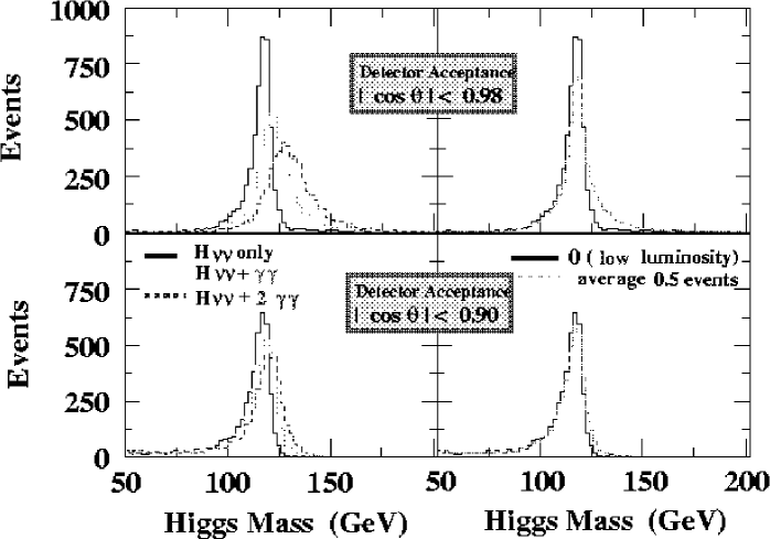
Figure 2.33: Distributions of the reconstructed mass of the Higgs in $\mbox{${\mathrm{e}}^{+}{\mathrm{e}}^{-}$}\mbox{$\rightarrow$}\nu\bar{\nu}\mbox{$\mathrm{h}^{0}$}$ process. Upper plots are for the mass with hits observed in the detector acceptance $|{\mathrm{cos\theta}}|\leq 0.98$, and bottom plots are for $\leq 0.90$. Left plots are those for none, one, two two-photon events overlapped. The dotted lines in the right side plots are the reconstructed mass in case 0.5 events are expected in average for the overlap.

In case two or more events happen in single bunch collision, the separation of the events is extremely difficult. The separation is almost impossible for the neutral particles like $\gamma$ or K_L. Some of the charged tracks might be rejected looking into the production point in beam direction, however such rejection might make significant bias in the Higgs precise measurements since the displaced vertex may come from the heavy quark decay of the Higgs.

Several simulation studies have been attempted. The simulation overlaps the hard scattering events of signal or background processes, with one or more two-photon events. We have used the JSF Quick-simulator [18] for this purpose. The data base are separately generated for the hard processes and the two-photon backgrounds. Afterward they are overlapped each other with event production points displaced according to the assumed beam spread at the interaction point. One of the significant effect is found in the reconstructed mass of the Higgs in $\mbox{${\mathrm{e}}^{+}{\mathrm{e}}^{-}$}\mbox{$\rightarrow$}\nu\bar{\nu}\mbox{$\mathrm{h}^{0}$}$ process.

Figure 2.33 shows the reconstructed mass with/without two-photon overlap. No event selection is made for the plots. The distributions are shown for the different detector acceptance to be used in the mass reconstruction. Since the two-photon background tends to make energy-flow in the forward region, the bias in the mass reconstruction could be reduced if we use the detector information only from the central part, while the signal tagging efficiency in a mass window is reduced as shown in the figure.

The effect on the signal tagging efficiencies is shown in Fig2.34. The vertical axis is the efficiency normalized to that without two-photon overlap. Significant degradation of the tagging efficiency is found. The main reason of the loss of the efficiency is the distorted mass distribution with overlapping two-photon events. Also the other kinematic values such as missing momentum direction are affected significantly. Furthermore the background contamination especially We$\nu$ events increases rapidly as two-photon overlap rate grows.

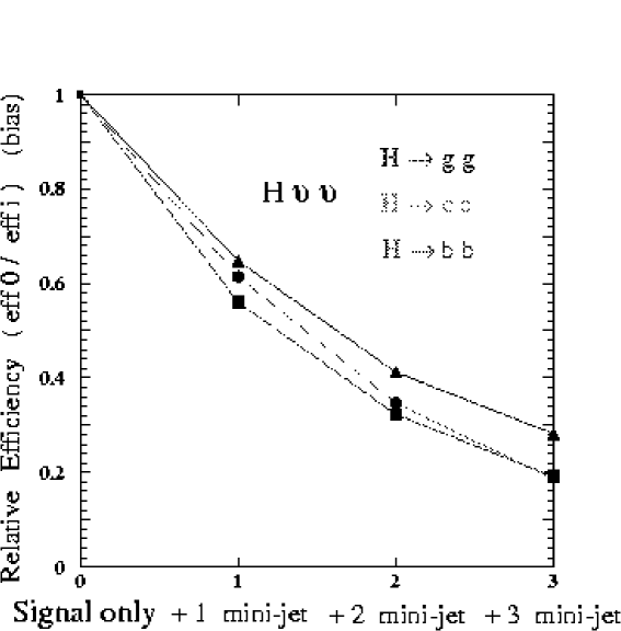
Figure 2.34: Degradation of the detection efficiency for the $\mbox{${\mathrm{e}}^{+}{\mathrm{e}}^{-}$}\mbox{$\rightarrow$}\mbox{$\mathrm{h}^{0}$}\nu\bar{\nu}$ process as a function of the number of two-photon processes overlapped to the signal event. Three lines correspond to different decay of the Higgs.

The other effect is that in the flavour tagging which relies on the tracks displaced from the event primary vertex. The overlapping event has, in general, its event-production-point different from the original event, since the beam has a finite width. If we use the information only in r-$\phi$ projection, the effect can be minimized thanks to the tiny width of the beam in the projection. However the beam spread is larger in the beam-direction. Simulation studies have been made also for the flavour tagging. Possible bias has been checked with different assumptions for the beam spread in beam direction. As we have expected, the effects are found to be negligible in r-$\phi$ projection. The results obtained in the 3-dimensional tagging show a small effects for 80 $\mu$m spread in z-direction at the interaction point which is the current design value at JLC. When we increase the beam spread, the bias increases almost linearly.

Although the studies have just started and the analyses are not optimized for the two-photon overlapping, the results indicate the several important issues for the accelerators, detectors and monitoring systems. Note that our aimed precisions for the Higgs measurements are percent order or less. We need good “time-stumps” for each hits in the detectors to identify the corresponding bunch. Both trackers and calorimetry are required to have good time resolution. Since the overlapping rate depends on the luminosity per bunch, the operation of the accelerators are required to be stable bunch by bunch, and the monitoring of the luminosity per bunch might be necessary. One may use the data at low luminosity to investigate the effects in real data, overlapping the hits from hard scattering events with minimum-bias events including two-photons. Many studies are addressed in the future.

Here we summarize the conclusion obtained so far.

• The effect of the two photon background can be minimized if we use the central part of the detector in order to avoid the bias due to two photon yields.

• The systematics can be minimized by the studies in data itself using the overlapping events in hit level for events obtained at lower luminosity data.

• The effects in flavour tagging needs care. For small beam size in beam direction in JLC the current design is good in order to avoid the bias. If we make larger $\sigma_{z}$, we may need special tricks to reject tracks from two-photon.

2.7.3 Requests to Detector

Through above discussion, here we list requests to detector design optimizations.

1. Vertex detector should have at least 4 layers, each with r-$\phi$ and z coordinates, in order to assure the local tracking capability.

2. To deal with two-photon overlap, the central tracker (CT) should have the bunch identification (time stamp) performance of 1 nsec.

3. It would be very helpful to have a fast detector for the intermediate tracker (IT) to help the bunch identification.

4. Calorimeter should have a time resolution of less than 1 nsec for a given hit. This request is very important especially for the endcap region. Granularity of the calorimeter also should be optimized.

Above requests are serious especially for high luminosity option of the JLC accelerator.

2.8 Future Studies to be Made

Here we summarize the the high priority studies which should be made in ACFA for JLC projects.

Physics channels

In this report we focus on the physics at JLC-I especially the SM Higgs and the lightest CP-even Higgs. Important channels which are not described in detail in this report are as follows.

• The Yukawa processes such as ${\mathrm{e}}^{+}{\mathrm{e}}^{-}$$\rightarrow$$\mathrm{t}\bar{\mathrm{t}}$$\rightarrow$$\mathrm{t}\bar{\mathrm{t}}$$\mathrm{h}^{0}$, and also heavier Higgs such as $\mathrm{t}\bar{\mathrm{t}}$$\mathrm{A}^{0}$ and $\mathrm{t}\bar{\mathrm{t}}$$\mathrm{H}^{0}$, have to be studied in detail.

• Multi-Higgs production such as $\mathrm{h}^{0}$$\mathrm{h}^{0}$$\mathrm{Z}^{0}$ and direct measurement of the self-coupling strength.

• The heavy Higgs pair production, $\mathrm{A}^{0}$$\mathrm{H}^{0}$.

• Charged Higgs in ${\mathrm{e}}^{+}{\mathrm{e}}^{-}$$\rightarrow$H⁺H^- and the single production such as $\mbox{${\mathrm{e}}^{+}{\mathrm{e}}^{-}$}\mbox{$\rightarrow$}\tau\nu\mbox{$\mathrm{H}^{\pm}$}$ [40].

These studies should be extended also at higher energies in a TeV and multi-TeV regions which is the one of the options at later stages of the JLC project.

Analyses Techniques

The sensitivity to Higgs bosons are determined not only by the accelerators and detectors but also the essential analyses techniques. The essential techniques are;

• Energy-flow calculation.

• Flavour tagging.

• tau tagging.

The current studies uses rather simple and old-fashion procedures. For example, in this study we use the simple likelihood calculation for the flavour-tagging based on the impact parameters of the tracks. At recent experiments like LEP/SLC, various more sophisticated methods with much higher performance have been developed using more information such as secondary vertex reconstruction. Multi-variables have been combined using neural-network techniques or likelihood combinations. These experience should be applied for the next steps. Above these crucial issues are under development and open for the future studies.

More studies in the real experimental situation

As we have described above, the experimental situation at JLC is much cleaner than the hadron colliders. We have described the effects of the beam-beam interaction and mini-jet (two-photon) event overlaps, which are major issues at high luminosity operation at JLC. As is discussed, these are expected not to be serious at JLC. In order to obtain better performance and feed-back to final designs of the accelerator and detector, further studies are addressed.

2.9 Summary

The future linear ${\mathrm{e}}^{+}{\mathrm{e}}^{-}$ collider, JLC, gives us fantastic occasions to investigate the physics up to GUT scale through studies of Higgs production and decay properties.

In this report we studied varieties of Higgs physics based on the recent progress in theoretical and experimental sides.

The experimental feasibilities and sensitivities are investigated especially for physics at early stage of the JLC phase-I. We discussed the sensitive signal cross-section, model-independent measurements, and expected accuracy in physics parameters such as Yukawa-coupling. Full simulation studies for the tracking as well as the effect of the event overlapping expected at JLC has been started already.

The existence of the light Higgs predicted in SUSY models is first to be clarified. At JLC, we may need only a few days to discover (at least one of) the Higgs bosons if the current design luminosity value of JLC is realized. There is always a potential for us to find unexpected “big things” through Higgs hunting and measurements even at very early stage of the JLC experiment.

We have enough sensitivity even to the worst case with the lowest cross-section in SUSY models. The physics background processes which have event topologies similar to those of Higgs signals have cross-section just one or two orders of magnitude higher than the signal. The backgrounds are well under control thanks to the well defined initial states, which is necessary for the precise measurement of the Higgs and in order to be sensitive to new particle production with tiny cross-section. We are sensitive to a cross-section down to 1 fb level. One can say, in other words, it is really a “big discovery” when we find no Higgs at JLC phase-I.

Varieties of discoveries are yet waiting for us. For instance, if Br$(\mbox{$\mathrm{h}^{0}$}\mbox{$\rightarrow$}\mbox{$\mathrm{b}\bar{\mathrm{b}}$})$/Br$(\mbox{$\mathrm{h}^{0}$}\mbox{$\rightarrow$}\tau\tau)$ is found to be different from $m_{b}^{2}/m_{\tau}^{2}$, all models belonging to SM or type-II 2HDM, such as SUSY models, are excluded. If Yukawa couplings of top and charm normalized to its mass are found to be different, we need completely new theory for the fermion generation. If the measured cross-section is smaller than the minimum cross-section [11, 12] expected in SUSY models, it means new physics further beyond SUSY between EW and GUT scale. We may discover CP-mixing in Higgs sector. We also may discover other Higgs with tiny cross-section at JLC even at phase-I.

Our purpose of the experiments at JLC is not only to judge the existence of the light Higgs, but also to measure the Higgs properties precise enough if it exists. We would measure the cross-section, the branching ratio, natural width in percent order or less in its error at JLC based on more than 10⁵ Higgs events in a few years running which results in the precise measurements of the Higgs gauge coupling and Yukawa-coupling, and furthermore derivation of Higgs self-couplings in multi-Higgs production. These can be made model independent fashion.

From these measurements, we further measure various model parameters, and test in the internal consistency. The precise values of the Higgs properties, we are also sensitive to a loop effect of new particles such as scaler top quark. The mass of the other Higgs and properties are indirectly measured if we missed it at JLC phase-I, and can be tested at the next step of the JLC. The information from LHC are also helpful. All of those, which are expected to be done only with the next e⁺e^- Linear Collider, JLC, are essential to give definite answers to physics models and to determine the fundamental structure of the interaction in nature up to GUT scale. JLC is a big step to definitely answer the question whether we live in SUSY world or SM-like world, or completely new unexpected world.

Table 2.11: Accuracy at $\sqrt{s}=$300, 400 and 500 GeV with ${\cal{L}}$=500 fb^-1 for 120 GeV CP-even Higgs at JLC. The Higgs boson of SM-like is used as an input.

$\sqrt{s}$	300 GeV	400 GeV	500 GeV
$\Delta\mbox{$m_{\mathrm{h}}$}$ (lepton-only)	80 MeV	—	—
$\Delta\mbox{$m_{\mathrm{h}}$}$	40 MeV	—	—
$\Delta\sigma/\sigma$ (lepton-only)	2.1%	2.5%	2.9%
$\Delta\sigma/\sigma$	1.3%	—	—
$\Delta(\sigma_{h\nu\bar{\nu}}\cdot$Br($\mathrm{b}\bar{\mathrm{b}}$)	2.0%	—	—
ZZH-coupling $\Delta$ZZH/ZZH	1.1%	1.3%	1.5%
WWH-coupling $\Delta$WWH/WWH	1.6%	—	—
$\Delta\Gamma_{\mbox{$\mathrm{h}^{0}$}}/\Gamma_{\mbox{$\mathrm{h}^{0}$}}$	5.5%	12%	16%
Yukawa coupling $\Delta\lambda/\lambda$
$\lambda_{b}$	2.8%	6.1%	8.1%
$\lambda_{\tau}$	3.5%	—	—
$\lambda_{c}$	11.3%	13%	15%
$\lambda_{b}/\lambda_{\tau}$	2.3%	—	—
$\lambda_{b}/\lambda_{c}$	11%	12%	14%
$\lambda_{up-type}$	4.1%	—	—
$\lambda_{down-type}/\lambda_{up-type}$	3.2%	—	—
$\Delta(\sigma\cdot$Br)/$(\sigma\cdot$Br)
$\mathrm{h}^{0}$$\rightarrow$$\mathrm{b}\bar{\mathrm{b}}$	1.1%	1.3%	1.7%
$\mathrm{h}^{0}$$\rightarrow$$\mathrm{W}^{+}\mathrm{W}^{-}$	5.1%	12%	16%
$\mathrm{h}^{0}$$\rightarrow$$\tau^{+}\tau^{-}$	4.4%	—	—
$\mathrm{h}^{0}$$\rightarrow$$\mathrm{c}\bar{\mathrm{c}}$+gg	6.3%	—	—
$\mathrm{h}^{0}$$\rightarrow$$\mathrm{c}\bar{\mathrm{c}}$	22%	23%	27%
$\mathrm{h}^{0}$$\rightarrow$gg	10%	11%	13%
$\mbox{$\mathrm{h}^{0}$}\mbox{$\rightarrow$}\gamma\gamma$	—	—	—
$\mbox{$\mathrm{h}^{0}$}\mbox{$\rightarrow$}\mbox{$\mathrm{Z}^{0}$}\gamma$	—	—	—

Chapter 3 Supersymmetry

3.1 Introduction

The existence of a light neutral Higgs boson strongly indicates supersymmetry but it is by no means a solid proof. It is definitely necessary to discover at least one supersymmetric particle to prove it. We have emphasized that there are a lot of chances to discover at least one SUSY particle at the JLC[1]. Although which is the first to be discovered is model-dependent, the SUSY search methods to be invoked at the JLC is largely model-independent and, once we find one SUSY particle, it will guide us to discover the next. More important than discoveries are the precision measurements of the masses and couplings of these SUSY particles, which can be carried out model-independently, thereby allowing us to test model assumptions. It should also be noted that the polarized electron beam will play an essential role, in the course of the SUSY searches and studies.

Basically, these statements made back in 1992[2] are still valid except for the fact that the only SUSY breaking scheme available at that time was the one exploiting gravity to transmit the spontaneous breaking of supersymmetry in some hidden sector to our world. In the past few years, there has been tremendous progress and now we have a set of different models for such SUSY breaking transmission. The subgroup’s first mission is thus to list up currently available SUSY breaking schemes and clarify their experimental implications. For theorists, this means to try to exhaust possible SUSY breaking mechanisms and examine their characteristic features in terms of collider phenomenology and, for experimentalists, this means to identify possible new signatures of SUSY and investigate their detectability at the JLC[3]. The other lines of studies carried out in the ACFA studies include reexamination of the simplifying assumptions we made in our past studies: studies of $R$-parity breaking phenomena and special corners of the parameter space leading to some experimentally difficult situation such as the lighter chargino decaying into a stau plus a neutrino[4].

As already stated, even more interesting than the mere discovery of SUSY particles are precision measurements of their masses and couplings. The past JLC studies assumed an integrated luminosity of a couple of tens of ${\rm fb}^{-1}$. Recent advance in accelerator physics has, however, opened up possibility of some really high luminosity which was unconceivable at the time of the green book being written[2]. The subgroup’s next task is thus to clarify what we can learn from first a couple of SUSY particles, given a real high integrated luminosity such as $1~{}{\rm ab}^{-1}$, quantify required precisions for model discrimination for various observables, and translate them into required detector performance.

In this chapter, we first quickly review the phenomenological consequences of various SUSY breaking scenarios and experimental expectations from the next generation colliders. We then perform simulated experiments in the framework of the minimal supersymmetric standard model, in order to demonstrate basic experimental techniques to study SUSY particles at the JLC: measurements of masses, mixings, and quantum numbers of SUSY particles. This will be followed by discussions on possible complications and ways out, expected for some particular corner of the parameter space or from the other scenarios including gauge or anomaly mediated SUSY breaking as well as $R$-parity violation. We then examine the physics demands on the detector performance. The precision measurements of SUSY particles at the JLC will serve as a telescope to look into physics at really high scale. We conclude this chapter by showing how and to what extent we can carry out this very ambitious program.

3.2 SUSY Breaking Scenarios

It is clear that the SUSY is a broken symmetry, if it exists at all. It should not arbitrarily be broken, however, as long as it is meant to solve the naturalness problem: only Soft Supersymmetry Braking (SSB) terms are allowed to tame the quadratic divergence of the Higgs mass correction. Phenomenologically viable models can thus be classified in terms of how the SSB takes place and how it is transmitted to our observable sector. In almost all of the models, SUSY is broken dynamically at a high scale and then this breaking is mediated to our low energy world. Various SSB parameters at the high scale of SUSY breaking are determined by the choice of the SSB mechanism and the mediation mechanism. Various theoretical and experimental considerations restrict the scale to a rather big range $10^{4}$ GeV $<$ $M_{SSB}$ $<$ $M_{Pl}$. The low energy values of the SUSY breaking parameters are then decided by evolving them back to the weak scale via renormalization group equations. Consequently the sparticle masses and, in cases where mixing occurs, even their couplings depend on the SSB mechanism. Once these low energy values of sparticle properties are measured, therefore, we can in principle point towards the physics at high scale and hence at the SUSY breaking mechanism.

As already mentioned, in the early days of SUSY model building there existed essentially only one class of models where the SSB is transmitted via gravity to the low energy world. The past few years changed the situation drastically and now we have a set of different models that include the following:

1)

Gravity mediated models that include (minimal) SUGRA (mSUGRA), (constrained) MSSM (cMSSM), etc., where supergravity couplings of the fields in the hidden sector with the SM fields are responsible for the SSB terms. The difference between mSUGRA and cMSSM lies in the fact that the former fixes the Higgsino mixing mass parameter $\mu$ by demanding the radiative breaking of the EW symmetry, while the latter leaves it as a free parameter. Both assume universality of the gaugino and sfermion masses at the high scale. These models always have extra scalar mass parameter $m_{0}^{2}$ which needs fine tuning so that the sparticle exchange does not generate FCNC effects, at an unacceptable level.

2)

Anomaly Mediated Supersymmetry Breaking (AMSB) models, for which supergravity couplings that induce mediation are absent and the SSB is caused by loop effects. The conformal anomaly, which is always present, generates the SSB terms and the sparticles acquire masses due to the breaking of scale invariance. Note that this contribution exists even in the case of mSUGRA/MSSM, but is much smaller in comparison with the tree level terms that exist in those models. This mechanism becomes a viable one for solely generating the SSB terms, when the quantum contributions to the gaugino masses due to the ‘superconformal anomaly’ can be large [6, 7], hence the name Anomaly mediation for them. The slepton masses in the simplest model of this kind are tachyonic and require some other SUSY breaking mechanism to obtain phenomenologically acceptable mass spectrum. One way to fix this problem is to introduce a scalar mass parameter $m_{0}^{2}$.

3)

Gauge Mediated Supersymmetry Breaking (GMSB) models [8], where the SSB is transmitted to the low energy world via a messenger sector through messenger fields which have gauge interactions. These models have no problems with the FCNC and do not involve any scalar mass parameter.

4)

Models where the SSB mediation is dominated by gauginos [9]. These models are based on the brane world scenarios, where the brane (our world) on which the matter particles and their superpartners live is separated in the bulk from the one that is responsible for the SUSY breaking. Consequently, the wave functions of the matter particles and their superpartners on the SUSY breaking brane are suppressed, whereas those of the gauginos are substantial, due to the fact that the gauge superfields live in the bulk. Hence the matter sector feels the effects of SUSY breaking dominantly via gauge superfields. As a result, in these scenarios, one expects $m_{0}\ll m_{1/2}$, reminiscent of the ‘no scale’ models.

All of these models clearly differ in their specific predictions for various sparticle spectra, features of some of which are summarized in Table 3.1[10], where the usual messenger scale parameter $\Lambda$ had been traded for $M_{2}$ for ease of comparison.

Table 3.1: Predictions of different types of SUSY breaking models for gravitino, gaugino, and scalar masses. $\alpha_{i}={g_{i}^{2}}/{4\pi}$ (i=1,2,3 corresponds to $U(1)$, $SU(2)$ and $SU(3)$, respectively), $b_{i}$ are the coefficients of the ${-g_{i}^{2}}/{(4\pi)^{2}}$ in the expansion of the $\beta$ functions $\beta_{i}$ for the coupling $g_{i}$ and $a_{i}$ are the coefficients of the corresponding expansion of the anomalous dimension. The coefficients $G_{i}$ are the squared gauge charges multiplied by various factors which depend on the loop contributions to the scalar masses in the different models.

Model	$m_{\tilde{G}}$	$(mass)^{2}$ for gauginos	$(mass)^{2}$ for scalars
mSUGRA	${{M_{SSB}^{2}}/{\sqrt{3}M_{pl}}}$ $\sim$ TeV	$({\alpha_{i}}/{\alpha_{2}})^{2}$ $M_{2}^{2}$	$m_{0}^{2}+\sum_{i}G_{i}M_{i}^{2}$
cMSSM	$M_{SSB}\sim 10^{10}-10^{11}$ GeV
GMSB	$({\sqrt{F}}/{100TeV})^{2}$ eV	$({\alpha_{i}}/{\alpha_{2}})^{2}M_{2}^{2}$	$\sum_{i}G_{i}^{{}^{\prime}}M_{2}^{2}$
	10 $<\sqrt{F}<10^{4}$ TeV
AMSB	$\sim$ 100 TeV	$({\alpha_{i}}/{\alpha_{2}})^{2}({b_{i}}/{b_{2}})^{2}M_{2}^{2}$	$\sum_{i}2a_{i}b{i}({\alpha_{i}}/{\alpha_{2}})^{2}M_{2}^{2}$

As one can see, the expected gravitino mass varies widely in different models. The SUSY breaking scale $\sqrt{F}$ in GMSB model is restricted to the range shown in the table by cosmological considerations. Since $SU(2)$ and $U(1)$ gauge groups are not asymptotically free, i.e., $b_{i}$ are negative, the slepton masses are tachyonic in the AMSB model, without a scalar mass parameter, as can be seen from the third column of the table. The minimal cure to this is, as mentioned before, to add an additional parameter $m_{0}^{2}$, not shown in the table, which however spoils the RG invariance. In the gravity mediated models like mSUGRA, cMSSM, and most of GMSB models, gaugino masses unify at high scale, whereas in the AMSB models the gaugino masses are given by RG invariant equations and hence are determined completely by the values of the couplings at low energies and become ultraviolet insensitive. Due to this very different scale dependence, the ratio of gaugino mass parameters at the weak scale in the two sets of models are quite different: gravity mediated models and GMSB models have $M_{1}:M_{2}:M_{3}$ = 1 : 2 : 7, whereas the AMSB model has $M_{1}:M_{2}:M_{3}$ = 2.8 : 1 : 8.3. The latter therefore, has the striking prediction that the lightest chargino $\tilde{\chi}^{\pm}_{1}$ and the lightest supersymmetric particle (LSP) $\tilde{\chi}^{0}_{1}$, are almost pure SU(2) gauginos and are almost mass-degenerate. The expected sparticle spectra in any given model can vary a lot. But still one can make certain general statements, e.g. the ratio of squark masses to slepton masses is usually larger in the GMSB models as compared to mSUGRA. In mSUGRA one expects the sleptons to be lighter than the first two generation squarks, the LSP is expected mostly to be a bino and the right-handed sleptons are lighter than the left-handed sleptons. On the other hand, in the AMSB models, the left- and right-handed sleptons are almost degenerate. The above mentioned degeneracy between $\tilde{\chi}_{1}^{\pm}$ and $\tilde{\chi}_{1}^{0}$ is lifted by the loop effects [11]. For $\Delta M$ = $m_{\tilde{\chi}_{1}^{\pm}}$ - $m_{\tilde{\chi}_{1}^{0}}$ $<$ 1 GeV, the phenomenology of the sparticle searches in AMSB models will be strikingly different from that in mSUGRA, MSSM, etc. In the GMSB models, the LSP is gravitino and is indeed ‘light’ for the range of the values of $\sqrt{F}$ shown in Table 3.1. The candidate for the next lightest sparticle, the NLSP, can be $\tilde{\chi}^{0}_{1}$, $\tilde{\tau}_{1}$, or $\tilde{e}_{R}$ depending on model parameters. The NLSP life time and hence the decay length of the NLSP in lab is given by $L=c\tau\beta\gamma\propto\frac{1}{(M_{NLSP})^{5}}$ $(\sqrt{F})^{4}$. Since the theoretically allowed values of $\sqrt{F}$ span a very wide range as shown in Table 3.1, so do those for the expected life time and this range is given by $10^{-4}$ $<$ c$\tau\gamma\beta$ $<$ $10^{5}$ cm. Since the crucial differences in different models exist in the slepton and the chargino/neutralino sector, it is clear that the leptonic colliders which can study these sparticles with the EW interactions, with great precision, can really play a crucial role in model discrimination.

The above discussion, which illustrates the wide ‘range’ of predictions of the SUSY models, also makes it clear that a general discussion of the sparticle phenomenology at any collider is far too complicated. This makes it even more imperative that we try to extract as much model independent information as possible from the experimental measurements. This is one aspect where the JLC can really play an extremely important role.

3.2.1 SUSY Questions to be Answered by Next Generation Colliders

The existence of a sparticle is a qualitative evidence for the existence of a supersymmetric part (${\cal L}_{SUSY}$) in the Lagrangian of the world (${\cal L}_{world}$). The Lagrangian of the world must contain, however, a soft SUSY breaking part (${\cal L}_{SSB}$), which determines masses and mixings of sparticles. As stressed above, this SSB part is believed to be determined by physics at high scale: such as GUT or Planck scale physics, and its studies will enable us to make a first realistic step towards the ultra-high energy physics. As illustrated in Fig. 3.1,

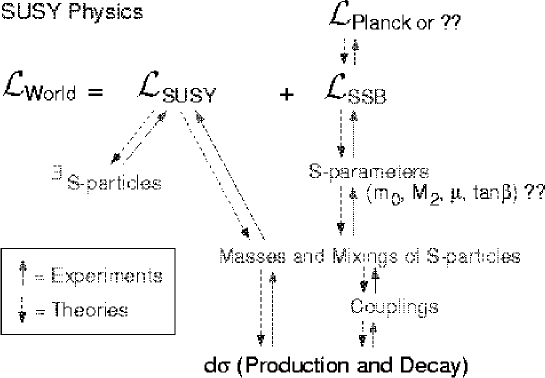
Figure 3.1: A schematic diagram showing the relation between the SUSY studies at the JLC and physics at high scale. The dashed arrows indicate the logical flow of theoretical implications, while the solid arrows show that of experimental inputs.

experimentalists’ tasks can, therefore, be summarized as follows: (i) search for a sparticle to qualitatively prove the existence of ${\cal L}_{SUSY}$, and (ii) determine masses and mixings of sparticles through the measurements of various differential cross sections, thereby testing SUSY quantitatively and uncovering the structure of ${\cal L}_{SSB}$. More specifically, we need to

• Find the sparticles and establish their quantum numbers by checking their interactions.

• Establish coupling equalities implied by the SUSY, thereby proving SUSY quantitatively.

• Determine the scalar masses, gaugino masses, and gaugino-higgsino mixing.

• Measure the properties of the third generation sfermions including the L-R mixing.

The measurements mentioned in (3) above can give information about $\mu$, $\tan\beta$, and some of the soft SUSY breaking parameters, whereas (4) above can further add to the determination of $\mu$, tan$\beta$, trilinear A parameters, and the scalar mass parameters.

The LHC will be able to achieve the goals given in ‘bold face’ in the list above; for the remaining tasks we need the clean environment of the $e^{+}e^{-}$ collider.

3.2.2 What LHC Can Do

Let us start with a summary of major hopes [12, 13, 14, 15] from the LHC for SUSY enthusiasts. Various versions of ‘naturalness’ arguments [16, 17, 18] indicate that if theories are ‘natural’, at least some of the sparticles, notably the gauginos/higgsinos, must be accessible at the LHC. Thus if SUSY is realized in nature, the LHC should be able to provide some proof for it.

Being a hadronic collider, the LHC is best suited for the search of strongly interacting particle sector. The heavier ‘strongly interacting’ sparticles will be produced first and the lighter sparticles with EW interactions only in the decay. The very high rates [19] (e.g., even for a gluino mass of 2 TeV, the expected cross-section is $\sim 10$ fb, giving about 1000 events for the high luminosity option) make discovery easy.

Methods have been developed to make accurate measurements of different sparticle masses; a nontrivial task as the worst background for SUSY searches is SUSY itself [20]. Depending on the point in mSUGRA parameter space chosen for analysis, a determination of $m_{\tilde{q}_{L}},m_{\tilde{g}}$ up to an accuracy of $5-7\%$ is possible, whereas the masses $m_{\tilde{\chi}^{0}_{1}},m_{\tilde{\chi}^{0}_{2}}$ can be determined with $<10\%$ accuracy [13, 14, 19, 20]. For some of the points chosen for studies high accuracies $\sim 1-2\%$ are also possible for neutralino mass determination. The heavier gauginos are, however, inaccessible in general since the rates for direct EW production are very low. The reach for sleptons at the LHC is also limited as compared to that for the strongly interacting particles and is $m_{\tilde{l}}$ $\leq$ 360 GeV unless it is produced in cascades of squarks; a model dependent fact. Their mass measurements are thus difficult, if not impossible. Ingenious methods have been developed to get an idea of the effective SUSY breaking scale [20]. However, accurate information about the SUSY breaking scale and mechanism generally does not seem easily extractable. Further, a direct determination of quantum numbers and couplings of the sparticles is not possible. It has been shown that many SUSY model parameters such as $\mu$, tan$\beta$, $M_{2}$, $M_{3}$ can be determined with an accuracy of a percent level [20, 21], within a model. However, model independent analyses do not yet promise similar accuracy [22].

There is another point to make. The lightest SUSY particle is a good candidate of the cold dark matter in the universe. It is thus desirable that collider measurements provide us with a clue about the nature of the dark matter. Such an analysis essentially needs determinations of the chargino/higgsino content of $\tilde{\chi}_{i}^{0}$ and the slepton masses. At the LHC, however, this is, so far, only shown to be possible for $m_{\tilde{l}_{R}}$ $<$ $m_{\tilde{\chi}_{2}^{0}}$[23]. On the other hand, a lepton collider can provide the necessary information on these sparticles, once produced, thereby making very crucial contributions. As a matter of fact, this information, if available, can play a very useful role in LHC analyses, too. Thus information obtained from the JLC can feed back into the LHC analyses.

3.2.3 What We Expect from JLC

The above discussion identifies the areas in which we expect significant contributions from the linear collider:

1)

The JLC should provide precision measurement of sparticle masses and mixing. Since the machine energy limits the sparticle spectrum that we can cover, it is desirable that the JLC shall eventually reach the TeV region.

2)

The linear collider should be able to pin down quantum numbers such as spin, hypercharge and establish the equality of couplings predicted by SUSY.

3)

Information from the LHC, along with measurements in (2) can then be used to get information about the SUSY breaking at high scale.

As seen before, the LHC can achieve the first goal only partially and the second one only indirectly. The information on sparticle masses obtained from the LHC can serve as an important input to guide energy upgrade strategy of the JLC. The tunable energy of the $e^{+}e^{-}$ linear collider allows for sequential production of various sparticles and hence a better control of the possible SUSY background to SUSY searches.

Since SUSY involves chiral fermions and their super-partners, The polarization of the initial $e^{+}$/$e^{-}$ beams can be used very effectively to project out information about sparticle spectra and couplings. Appropriate choice of the polarization can also reduce effectively the background due to $W^{+}W^{-}$ production which has a very high rate. Fig. 3.2 taken from Ref. [24] shows the

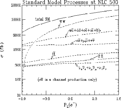
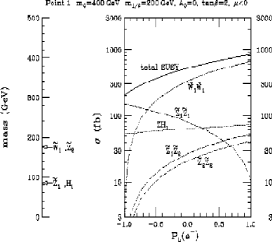
Figure 3.2: Cross sections of different SM processes as well as the chargino/neutralino production. Model parameter values are shown in the figure.

cross-sections for different SM processes and the corresponding ones for the SUSY model dependent chargino/neutralino pair production, at a chosen point in the mSUGRA parameter space. From the figure it is clear that with a judicious choice of polarization of $e^{-}$/$e^{+}$ beam, the SM background can be handled and precision measurements of chargino/neutralino sector are possible. The $e^{+}e^{-}$ collider produces democratically all the sparticles that have EW couplings. Hence it is better suited than the LHC to study the gauginos/higgsinos and sleptons and will complement the information in these sectors from the LHC very effectively. The correlation between properties of gluino that will be obtained from the LHC and those of chargino/neutralino sector from LHC/JLC can disentangle the various gaugino mass parameters $M_{i}$ at weak scale. For reasons outlined above knowledge about the relative values of $M_{i}(i=1,3)$ at the weak scale, from independent sources, contains crucial clues to the physics at high scale. This also shows how truly the LHC and the JLC are complementary to each other and thus how necessary both are to solve the puzzle of EWSB.

3.3 Simulated Experiments

3.3.1 Model Assumptions

To be specific, we will work within the framework of supergravity (SUGRA) models with the “GUT-condition”s, although the search and study methods are largely model-independent. These models involve, in general, the following parameters: ($m_{0}$, $M_{2}$, $\mu$, $\tan\beta$), which determine the mass spectra and the interactions of supersymmetric particles[26]. $\mu$ is the higgsino mixing mass parameter and $\tan\beta$ is the ratio of the two vacuum expectation values of two Higgs doublets. $m_{0}$ is the scalar mass parameter, which is common to all the scalar particles in the case of SUGRA models. $M_{2}$ is the $SU(2)$ gaugino mass parameter, which is related to the $SU(3)$ and $U(1)$ gaugino mass parameters:

$${M_{1}\over{5\over 3}\alpha/\cos^{2}\theta_{W}}={M_{2}\over\alpha/\sin^{2}\theta_{W}}={M_{3}\over\alpha_{s}}$$

under the GUT conditions. As already mentioned in the previous section, this means, numerically,

$$\begin{array}[]{lll}M_{1}:M_{2}:M_{3}\simeq 1:2:7,\end{array}$$ (3.1)

which implies the following inequality between the lighter chargino and the gluino masses:

$$\begin{array}[]{lll}m_{\tilde{\chi}^{\pm}_{1}}\hbox{ \raise 3.0pt\hbox to0.0pt{$<$}\raise-3.0pt\hbox{$\sim$} }\frac{1}{3}m_{\tilde{g}}.\end{array}$$ (3.2)

As demonstrated later, these SUGRA-GUT assumptions can be tested to a high precision.

On the other hand, sfermion masses can be written in the form:

$$\begin{array}[]{lll}m_{\tilde{f}}^{2}=m_{0}^{2}+G_{\tilde{f}}M^{2}+D_{\tilde{f}}m_{Z}^{2},\end{array}$$ (3.3)

where the first term on the right-hand side is the contribution from the common scalar mass ($m_{0}$). The coefficient of the gauge term ($G_{\tilde{f}}$) is controlled by the size of the gauge group to which the sfermion belongs and the coefficient of the $D$-term ($D_{\tilde{f}}$) depends on $\tan\beta$ and is of $O(1)$ or less. When $M_{2}^{2}\gg m_{Z}^{2}$, the sfermion mass spectrum is thus largely determined by the gauge term in the gravity-mediated SUSY breaking models. Taking into account the above two mass relations (Eqs.(3.2) and (3.3)), we can conclude that colored sparticles are heavier than colorless ones and right-handed sfermions are lighter than left-handed ones, in the gravity-mediated SUSY breaking models.

In order to avoid unnecessary complications, we will make the following simplifying assumptions: a) the $R$-parity is exactly conserved which implies that SUSY particles can only be pair-produced and the lightest SUSY particle (LSP) is absolutely stable and b) the LSP is the lightest neutralino to be consistent with cosmology. Complications expected when these simplifying assumptions are lifted and possible ways out will be discussed later. Our first SUSY particle (FSP) candidates are thus the lighter chargino ($\tilde{\chi}^{\pm}_{1}$) or the right-handed sleptons ($\tilde{l}^{\pm}_{R}$), except for the light third generation case. The low lying SUSY particles accessible for the JLC usually have a reasonable branching fraction for direct decays into the LSP[27]. Therefore, the signal for SUSY particle productions is a missing transverse momentum or a large acoplanarity.

Taking these into account, we will focus our attention on chargino and slepton pair productions. In any case, it is usually straightforward to discover these SUSY particles at the JLC, once their thresholds are crossed. Moreover, we will be able to study their properties in detail. It should be emphasized that detailed studies of the first SUSY particle alone can teach us a lot about the model parameters and will guide us to the discovery of the next.

In what follows we will demonstrate how a typical SUSY study program goes[28], taking a sample case:

$$(m_{0},M_{2},\mu,\tan\beta)=(70~{}{\rm GeV},250~{}{\rm GeV},400~{}{\rm GeV},2)$$

unless otherwise stated. This parameter set gives the following sparticle mass spectrum:

$$(m_{\tilde{\chi}^{0}_{1}},m_{\tilde{\chi}^{0}_{2}},m_{\tilde{\chi}^{\pm}_{1}},m_{\tilde{l}_{R}},m_{\tilde{l}_{L}},m_{\tilde{\nu}_{L}})=(118,222,220,142,236,227)~{}{\rm GeV}.$$

Thus the first SUSY particle (FSP) in this case is the right-handed sleptons pair-produced in $e^{+}e^{-}$ collisions. The third generation sleptons will be treated separately, since for them we expect significant left-right mixing.

3.3.2 Study of $\bf\tilde{\it l}^{\pm}_{\it R}({\it l}\neq\tau)$

Slepton Signature

Since a right-handed slepton decays directly into a lepton plus an LSP, the signal to look for is an acoplanar lepton pair: $e^{+}e^{-}\to\tilde{l}^{+}_{R}\tilde{l}^{-}_{R}\to l^{+}\tilde{\chi}^{0}_{1}l^{-}\tilde{\chi}^{0}_{1}$. On the other hand, the background to this reaction is standard model (SM) processes with neutrinos which mimic the LSP. The key point here is the power of a highly polarized electron beam available only at linear colliders. For instance, one can eliminate the largest SM background ($e^{+}e^{-}\to W^{+}W^{-}$ with $W\to l\nu$) very effectively, using a right-handed electron beam: the transverse $W$-pair production vanishes in the symmetry limit since the $s$-channel diagram involves a $W_{3}$, the third component of the $SU(2)_{L}$ gauge multiplet, and the $t$-channel diagram exchanges a $\nu_{e}$, both of which only couple to left-handed electrons. On the other hand, the signal cross section will be enhanced because of the weak hypercharge difference between $e^{-}_{L}$ and $e^{-}_{R}$: $\sigma_{R}=4\sigma_{L}$ in the symmetry limit. Figs. 3.3-a) and -b) are examples of acoplanarity distributions for selectron and smuon pair productions, respectively, after the accumulation of $20~{}{\rm fb}^{-1}$ at $\sqrt{s}=350~{}{\rm GeV}$.

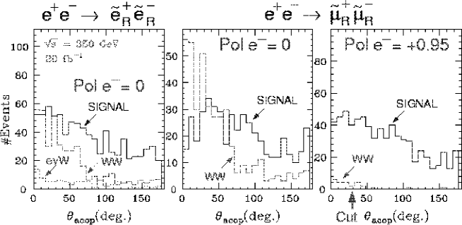
Figure 3.3: Examples of acoplanarity distributions for (a) selectron pair and (b) smuon pair productions. The Monte Carlo data correspond to an integrated luminosity of $20~{}{\rm fb}^{-1}$ at $\sqrt{s}=350~{}{\rm GeV}$ with an unpolarized electron beam. The solid histograms are for the signal events, while the dashed histograms are the background from $W^{+}W^{-}$ productions. The effect of the right-handed electron beam is demonstrated in (c).

We can see that the signals can be effectively enhanced over the background mainly consisting of $W$ pairs, by applying a cut on the acoplanarity angle. A detection efficiency of $\epsilon\hbox{ \raise 3.0pt\hbox to0.0pt{$>$}\raise-3.0pt\hbox{$\sim$} }50~{}\%$ is easily achieved with a signal to background ratio of $S/B\hbox{ \raise 3.0pt\hbox to0.0pt{$>$}\raise-3.0pt\hbox{$\sim$} }1.6$ even for smuons. As stressed above, the signal to background ratio can be further improved by using a right-handed electron beam as shown in fig. 3.3-c), resulting in a very clean event sample suitable for precision studies.

Mass Determination

Using this clean sample, we can determine the masses of the LSP and the right-handed slepton through the measurement of the final-state lepton energy distribution. The two-body decay of any spinless particle gives a flat energy distribution with its end points kinematically fixed by the masses of the parent and the daughter particles: in the case of the slepton decay, the slepton and the LSP masses:

$$E_{min} = \frac{m_{\tilde{\mu}_{R}}}{2}\left(1-\frac{m_{\tilde{\chi}^{0}_{1}}^{2}}{m_{\tilde{\mu}_{R}}^{2}}\right)\gamma(1-\beta)$$ (3.4)

$$E_{max} = \frac{m_{\tilde{\mu}_{R}}}{2}\left(1-\frac{m_{\tilde{\chi}^{0}_{1}}^{2}}{m_{\tilde{\mu}_{R}}^{2}}\right)\gamma(1+\beta),$$ (3.5)

where $\gamma=E_{beam}/m_{\tilde{\mu}_{R}}$ and $\beta=\sqrt{1-(m_{\tilde{\mu}_{R}}/E_{beam})^{2}}$.

Fig. 3.4-a) is the energy distribution of muons from smuon decays for an integrated luminosity of $20~{}{\rm fb}^{-1}$ with a right-handed electron beam. Though the distribution is a little bit different from the expected rectangular shape due, primarily, to selection cuts, the lower and the higher edges are sharp enough. These end points of the energy spectrum determine $m_{\tilde{\mu}}$ and $M_{\tilde{\chi^{0}_{1}}}$. Fig. 3.4-b) shows the contours obtained from the fit to the Monte Carlo data.

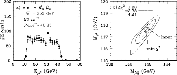
Figure 3.4: (a) The energy distribution of muons from smuon decays for the same Monte Carlo parameters as with Fig.3.3-b). The solid line corresponds to the best fit curve, letting $m_{\tilde{\mu}_{R}}$ and $m_{\tilde{\chi}^{0}_{1}}$ move freely. (b) The contours in the $m_{\tilde{\mu}}$-$M_{\tilde{\chi}^{0}_{1}}$ plane obtained from the fit to the energy distribution.

We can determine the smuon and the LSP masses to a 1% level.

Test of Generation Independence of Sfermion Masses

With the right-handed selectron and smuon masses determined this way, we can make a very important test of the SUSY breaking sector, which is a test of generation independence of sfermion masses.

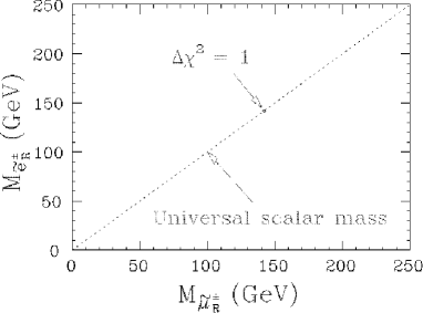
Figure 3.5: The expected $\Delta\chi^{2}=1$ contour in the $m_{\tilde{\mu}_{R}}$-$m_{\tilde{e}_{R}}$ plane.

The gravity-mediated SUSY breaking implies the universality of scalar masses at the GUT scale, which leads to the mass degeneracy of the first and the second generations. Fig. 3.5 is an example of the test of the generation independence, demonstrating potential precision available at the JLC.

Measurements of Differential Cross Sections

Now that we know the masses of the LSP and the sleptons, we can solve kinematics up to 2-fold ambiguities.

                

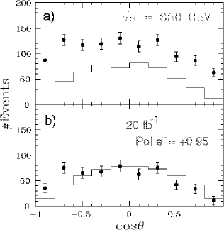
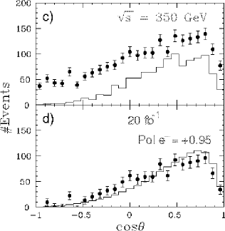
Figure 3.6: (a) Production angle distribution of $\tilde{\mu}^{-}_{R}$ with respect to the electron beam axis. The points with error bars are the distribution of the two solutions reconstructed from the selected sample corresponding to Fig. 3.4-a). The histogram is the generated $\cos\theta$ distribution for the selected sample. (b) Production angle distribution after the background subtraction compared with the scaled generated distribution before selection cuts. No acceptance correction is applied to the reconstructed distribution. (c) and (d) are similar plots to (a) and (b) for $e^{+}e^{-}\to\tilde{e}^{+}_{R}\tilde{e}^{-}_{R}$.

Fig. 3.6-a) plots the two solutions for the cosine of the smuon production angle. Comparison of this with the corresponding generated one (histogram) suggests that the wrong solution makes a flat background. After the background subtraction, we get the plot in Fig. 3.6-b), which shows a $\sin^{2}\theta$ distribution characteristic of $s$-channel pair productions of a spinless particle. In this way we can confirm that our smuon is really a scalar particle.

On the other hand, the right-handed selectron pair production has $t$-channel neutralino-exchange diagrams in addition. Notice that only their bino ($\tilde{B}$) components contribute here, since the wino component does not couple to the right-handed sleptons and the higgsino couplings are proportional to the electron mass. The $t$-channel diagram, if active, will produce a forward peak if significant. Figs. 3.6-c) and -d) are similar plots to Figs. 3.6-a) and -b) for the right-handed selectron pair production. The forward peak indicates that the LSP in our sample case is bino-dominant. The JLC’s polarized electron beam will, again, play a crucial role here since the $t$-channel diagrams exist only for the selectron with the same chirality as the beam electron.

Test of Supersymmetry

Up to now, we have been implicitly assuming that the discovered sparticles obey supersymmetry. In this subsection, we turn our attention to how we can quantitatively test supersymmetry.

Supersymmetry not only demands existence of a super-partner for each of the standard model particles but also requires the supersymmetric relations among couplings that are related by supersymmetry. Because of this, the fermion-sfermion-gaugino coupling, for instance, has the following relation with the fermion-fermion-gauge coupling in the lowest order of perturbation theory:

$$g_{\tilde{B}\tilde{e}_{R}e_{R}} =\sqrt{2}g\tan\theta_{W}=\sqrt{2}g^{\prime},$$ (3.6)

If we can test such a SUSY relation, we can quantitatively prove that there is indeed supersymmetry in nature. Here, we discuss to what extent we can test the SUSY relation for the $e$-$\tilde{e}_{R}$-$\tilde{B}$ coupling, using the selectron pair production.

Let us parametrize the deviation of this coupling from the gauge coupling as

$$g_{\tilde{B}\tilde{e}_{R}e_{R}}=\sqrt{2}g^{\prime}Y_{\tilde{B}},$$

and consider the constraint on $Y_{\tilde{B}}$ from the $\tilde{e}_{R}\tilde{e}_{R}$ production. In the limit that the beam energy is high enough and the neutralino mixing is negligible: $\sqrt{s}\gg m_{Z}$ and $M_{1}\ll\mu$, The $\tilde{e}_{R}$ pair production amplitude can be written in the form:

$${\cal M}\propto\sin\theta\left[1-\frac{4Y^{2}_{\tilde{B}}}{1-2\cos\theta\beta_{f}+\beta_{f}^{2}4M_{1}^{2}/s}\right],$$

where $\theta$ is the selectron production angle measured from the electron beam axis. Notice that the $s$($t$)-channel particle that contributes to the right-handed selectron pair production is only $B$ ($\tilde{B}$), and consequently the cross section only depends on the hyper-charge.

The formula tells us that we can constrain $Y_{\tilde{B}}$ by measuring the differential cross section: $d\sigma(e^{+}e^{-}\rightarrow\tilde{e}^{+}_{R}\tilde{e}^{-}_{R})/d\cos\theta$ (we have already demonstrated that the selectron production angle can be reconstructed from the daughter $e^{+}$ and $e^{-}$ momenta. Fig.3.7 is the constraint shown in the $M_{1}$-$Y_{\tilde{B}}$ plane from Monte Carlo data sample corresponding to 100 fb^-1. We used the information on the selectron and the neutralino masses, and the selectron differential cross section, and assumed the GUT relation between $M_{1}$ and $M_{2}$.

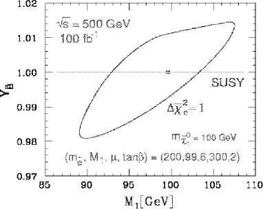
Figure 3.7: The $\Delta\chi^{2}=1$ contour in the $M_{1}$-$Y_{\tilde{B}}(\equiv g_{\tilde{B}\tilde{e}_{R}e}/g^{\prime}\sqrt{2})$ plane for pairs of $\tilde{e}_{R}$ with a mass of 200 GeV generated at $\sqrt{s}=500$ GeV with $\int Ldt=100fb^{-1}$. Input parameters are $\mu=300$ GeV, $M_{1}=99.57$, and $\tan\beta=2$.

Notice that once we find the charginos or the other neutralinos, we can use them to constrain the ino mass matrices, and further improve the constraint on $Y_{\tilde{B}}$ and other couplings.

On the other hand, $Y_{\tilde{B}}=1$ holds only at the lowest order of perturbation and is expected to deviate from $1$ through radiative corrections. In the case of $m_{\tilde{q}}\gg m_{\tilde{l}}$, the sizes of the radiative corrections are

$$\delta Y_{\tilde{B}\tilde{e}_{R}e} \sim 0.007\log_{10}(m_{\tilde{q}}/m_{\tilde{l}})$$ (3.8)

$$\delta Y_{\tilde{W}\tilde{\nu}e} \sim 0.02\log_{10}(m_{\tilde{q}}/m_{\tilde{\nu}})$$ (3.9)

and their effects on the cross sections are expected to be 2.8% and 8.2%, respectively, for $m_{\tilde{q}}/m_{\tilde{\nu}}\sim 10$. If we have enough statistics for $\tilde{e}_{L,R}$, $\tilde{\nu}_{L}$ we can thus put some limit on $m_{\tilde{q}}$ through the measurements of the sizes of the radiative corrections.

3.3.3 Study of $\bf\tilde{\chi}^{\pm}_{1}$

The charginos $\chi_{1}^{\pm}$, $\chi_{2}^{\pm}$ are the mixtures of charged wino $\tilde{W}^{\pm}$ and charged higgsino $\tilde{H}^{\pm}$ obtained from the diagonalization of the mass matrix

$${\cal L}_{\rm mass}=(\tilde{W}^{+}~{}~{}\tilde{H}^{+})\pmatrix{M_{2}&\sqrt{2}m_{W}\cos\beta\cr\sqrt{2}m_{W}\sin\beta&\mu\cr}\pmatrix{\tilde{W}^{-}\cr\tilde{H}^{-}\cr}.$$ (3.10)

Notice that this mass matrix is given in terms of the three SUSY parameters: ($M_{2}$, $\mu$, $\tan\beta$) of which $M_{2}$ and $\mu$ mainly control the mixing between the weak eigenstates. When the splitting between $M_{2}$ and $\mu$ is large, the mixing is small and the pure states, the charged wino and higgsino, essentially become mass eigenstates.

From the slepton studies, we can determine the mass of the LSP($\tilde{\chi}^{0}_{1}$) to better than 1 %. From this and the mass formula above, we can set an upper limit on the lighter chargino mass, assuming the GUT relation among the gaugino mass parameters. This upper limit corresponds to the gaugino-dominant case ($m_{\tilde{\chi}^{\pm}_{1}}\simeq 2\times m_{\tilde{\chi}^{0}_{1}}$), while the LSP and the lighter chargino will be almost mass-degenerate in the higgsino-dominant case. The upper limit is plotted in Fig. 3.9 as a function of the LSP mass.

Chargino Signature

We thus set our center of mass energy just above $4\times m_{LSP}$ and look for $\tilde{\chi}^{\pm}_{1}$ pair productions. In our sample case, the chargino decays into a real $W$ and an LSP ($\tilde{\chi}^{\pm}_{1}\to W^{\pm}\tilde{\chi}^{0}_{1}$).

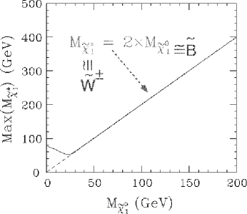
Figure 3.8: Upper limit on the lighter chargino mass as a function of the LSP mass, assuming the GUT relation.

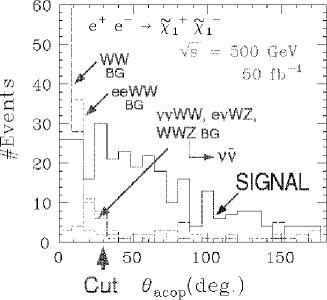
Figure 3.9: Acoplanarity angle distribution for $e^{+}e^{-}\to\tilde{\chi}^{+}_{1}\tilde{\chi}^{-}_{1}$ together with major standard-model backgrounds.

The signal to look for will thus be an acoplanar $W$ pair in 4-jet final states. Fig. 3.9 shows the acoplanarity angle distribution for the signal events (solid histogram) together with major standard-model backgrounds: the $W^{+}W^{-}$ (dash), the $e^{+}e^{-}W^{+}W^{-}$ (dot), and the sum of the $e^{\pm}\mathop{\nu_{e}}\limits^{\mbox{\tiny$(-)$}}W^{\mp}Z^{0}$, $W^{+}W^{-}Z^{0}$, and $\nu_{e}\bar{\nu}_{e}W^{+}W^{-}$ (dot-dash) productions, after demanding two $W$ candidates in the final states. A cut at $\theta_{A}=30^{\circ}$ will give us a fairly clean sample with a selection efficiency in excess of $10~{}\%$ including the branching fraction to the 4-jet final states.

Mass Determination

As we did to the sleptons, we can first use this clean sample to determine the chargino mass.

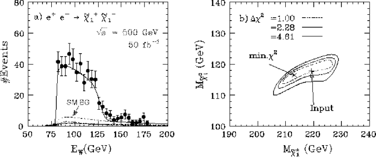
Figure 3.10: (a) Energy distribution of final-state $W$’s from chargino decays: $\tilde{\chi}^{\pm}_{1}\to W^{\pm}\tilde{\chi}^{0}_{1}$ (points with error bars) for the sample shown in Fig. 3.9 after the acoplanarity angle cut at $\theta_{A}=30^{\circ}$. The solid curve is the best-fit curve to determine $m_{\tilde{\chi}^{\pm}_{1}}$ and $m_{\tilde{\chi}^{0}_{1}}$. The other curves correspond to the histograms in Fig. 3.9. (b) Resultant contours from the 2-parameter fit.

Fig. 3.10-a) plots the expected energy distribution of the final-state $W$’s from the chargino decays. The solid curve is the best-fit curve from a 2-parameter fit letting the $m_{\tilde{\chi}^{\pm}_{1}}$ and $m_{\tilde{\chi}^{0}_{1}}$ move freely. Notice that the fit includes the standard-model backgrounds shown as dashed, dot-dashed, and dotted curves, corresponding to those in Fig. 3.9. Fig. 3.10-b) is the resultant contour plot in the $m_{\tilde{\chi}^{\pm}_{1}}$-$m_{\tilde{\chi}^{0}_{1}}$ plane, which tells us that we can determine the chargino mass to $\Delta m_{\tilde{\chi}^{\pm}_{1}}\simeq 8~{}{\rm GeV}$. If we use the LSP mass constraint from the slepton study, we can improve this to $\Delta m_{\tilde{\chi}^{\pm}_{1}}\simeq 5~{}{\rm GeV}$.

Measurement of Differential Cross Section

The clean sample can also be used to study the angular distribution of $\tilde{\chi}_{1}^{\pm}$’s as has been done to the right-handed slepton-pair production. One can determine the four-momenta of the charginos up to a two-fold ambiguity, once their masses are known. Fig.3.11-a) plots the angular distribution with the two-fold ambiguity unresolved.

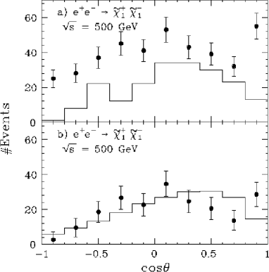
Figure 3.11: (a) An example of the reconstructed production angle distribution (data points) compared with the generated angle distribution of the selected sample (histogram). The Monte Carlo events were generated at $\sqrt{s}=500~{}{\rm GeV}$ and correspond to an integrated luminosity of $50~{}{\rm fb}^{-1}$. We have assumed a $100\%$ charge ID efficiency for $W$’s here. The two solutions were plotted in the same figure. (b) Same as (a) but after the subtraction of the background due to wrong solutions. The histogram is the scaled generated angle distribution for the initial sample before selection cuts, while the data points are the reconstructed without acceptance correction.

The “wrong” solutions again give an almost flat distribution, which can be subtracted to reproduce the real angular distribution as shown in Fig.3.11-b). The event excess in the forward region suggests that there is some diagram with $t$-channel particle exchange. The only particle exchanged in the $t$-channel here is the electron sneutrino $\tilde{\nu}_{e_{L}}$.

Test of SUGRA-GUT Relation

More interesting is the measurement of the production cross section for the polarized electron beam. Notice that, for the right-handed electron beam, only higgsino components contribute to the chargino pair production in the symmetry limit, since the gauge boson exchanged in the $s$-channel is $B$ ($U(1)_{Y}$ gauge boson), while the $t$-channel sneutrino exchange diagram is absent. By measuring the production cross section for the right-handed electron beam, we can thus determine the composition of $\tilde{\chi}^{\pm}_{1}$.

We now know the LSP ($\tilde{\chi}^{0}_{1}$) and the chargino ($\tilde{\chi}^{\pm}_{1}$) masses, which constrain the chargino and neutralino mass matrices, the production cross section for $e^{+}e^{-}_{R}\to\tilde{e}^{+}_{R}\tilde{e}^{-}_{R}$, which depends on the bino component of the LSP, and the production cross section for $e^{+}e^{-}_{R}\to\tilde{\chi}^{+}_{1}\tilde{\chi}^{-}_{1}$, which provides information on the chargino composition. Combining these measurements together, we can carry out a global fit to determine SUSY breaking parameters: $(M_{1},M_{2},\mu,\tan\beta)$. Notice that we did not assume the GUT relation between $M_{1}$ and $M_{2}$ here, thereby testing it to get insight into the SUSY breaking mechanism. Fig. 3.13 is the result from such a global fit to Monte Carlo data generated with the GUT relation indicated as a dashed line. In this way, we can test the GUT relation.

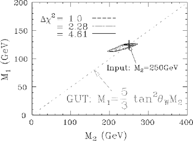
Figure 3.12: Constant $\chi^{2}$ contours in the $M_{2}$-$M_{1}$ plane obtained from the global fit explained in the text. The dotted line shows the GUT relation.

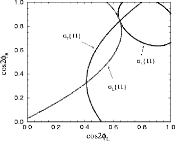
Figure 3.13: Contours of the cross sections $\sigma_{L}\{11\}$, $\sigma_{R}\{11\}$ and $\sigma_{T}\{11\}$ in the $\cos 2\phi_{L}$-$\cos 2\phi_{R}$ plane for $\tan\beta=3,m_{0}=100~{}{\rm GeV},M_{1/2}=200~{}{\rm GeV}]$ at $\sqrt{s}=400$ GeV[29].

Full Reconstruction of the Chargino Mass Matrix

The analysis presented above can be worked out further[29] to fully reconstruct the chargino mass matrix given by Eq. (3.10), which we repeat here for convenience:

$${\cal M}_{C}=\pmatrix{M_{2}&\sqrt{2}m_{W}\cos\beta\cr\sqrt{2}m_{W}\sin\beta&\mu}$$

Notice that the mass matrix, being asymmetric, requires two unitary matrices for diagonalization. We thus have two (real) mixing angles, $\phi_{L}$ and $\phi_{R}$, which are given in terms of $M_{2}$, $\mu$, and $\tan\beta$. These SUSY parameters are, in general, complex, implying a possible non-trivial $CP$ phase which cannot be removed by field redefinitions. Without loss of generality, we can attribute this phase to the $\mu$ parameter.

As mentioned above, only the $s$-channel $B$ exchange diagram contribute to $e^{+}e^{-}_{R}\to\tilde{\chi}^{+}_{1}\tilde{\chi}^{-}_{1}$, thereby singling out the higgsino component of the chargino. Because of this the corresponding cross section ($\sigma_{R}\{11\}$) is symmetric with respect to $\cos 2\phi_{L}$ and $\cos 2\phi_{R}$ and is independent of the mass of the sneutrino that could be exchanged in the $t$-channel if the electron beam were left-handed On the other hand, the left-handed ($\sigma_{L}\{11\}$) and the transverse ($\sigma_{T}\{11\}$) cross sections vary with the sneutrino mass and the $e\tilde{\nu}\tilde{W}$ Yukawa coupling ($g_{e\tilde{\nu}\tilde{W}}$). When mapped into the $\cos 2\phi_{L}$-$\cos 2\phi_{R}$ plane, these cross sections comprise elliptic or parabolic contours, which may cross each other up to four times. Remember that $\sigma_{R}\{11\}$ is invariant against any change of $m_{\tilde{\nu}_{e}}$ or $g_{e\tilde{\nu}\tilde{W}}$, while $\sigma_{L}\{11\}$ and $\sigma_{T}\{11\}$ move with them. Since the three cross section measurements meet at a single point in the $\cos 2\phi_{L}$-$\cos 2\phi_{R}$ plane only for the correct solution, we can thus decide the mixing angles by changing $m_{\tilde{\nu}_{e}}$ provided that the $e\tilde{\nu}\tilde{W}$ Yukawa coupling is identified with the gauge coupling as dictated by the supersymmetry. Fig. 3.13 demonstrate this.

Instead of using beam polarizations, we can also use the final-state polarization of charginos, which can be extracted by measuring the distributions of their decay daughters. It has been shown that we can reconstruct the polarization vectors of the charginos and their spin-spin correlation tensor dynamics-independently, and use them to decide the mixing angles[29]. Note also that these additional measurements, including the differential cross section measurements, can be used, in combination with the beam polarizations, to check the equality of the $e\tilde{\nu}\tilde{W}$ Yukawa coupling to the gauge coupling (a quantitative test of supersymmetry)[31].

When the machine energy reaches the pair production threshold for the heavier chargino, we will be able to study all of the three combinations:

$$e^{+}e^{-} \to \tilde{\chi}^{+}_{1}\tilde{\chi}^{-}_{1}$$

$$\to \tilde{\chi}^{+}_{1}\tilde{\chi}^{-}_{2}$$ (3.11)

$$\to \tilde{\chi}^{+}_{2}\tilde{\chi}^{-}_{2}.$$ (3.12)

This will allow us to measure the masses of the two charginos, the production cross sections for the left- and right-handed electron beams for the three processes, and various decay distributions. These measurements can then be use to unambiguously determine all of the chargino mass matrix parameters, including $CP$ phase. Figure 3.14

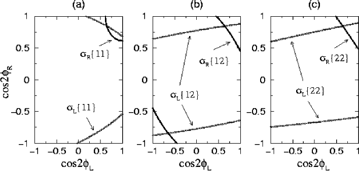
Figure 3.14: Contours of the cross sections (a) $\sigma_{L/R}\{11\}$, (b) $\sigma_{L/R}\{12\}$, and (c) $\sigma_{L/R}\{22\}$ in the $\cos 2\phi_{L}$-$\cos 2\phi_{R}$ plane for $\tan\beta=3,m_{0}=100~{}{\rm GeV},M_{1/2}=200~{}{\rm GeV}]$ at $\sqrt{s}=800$ GeV[29].

shows the cross section contours in the $\cos 2\phi_{L}$-$\cos 2\phi_{R}$ plane for the three processes with different beam polarizations. We can see that the three figures uniquely select a single point $(\cos\theta_{L},\cos\theta_{R})=(0.645,0.844)$ in the mixing angle plane. In this way, we can thus decide the mixing angles with a statistical error of a percent level or better, given an integrated luminosity of $1~{}{\rm ab}^{-1}$. Notice also that the mass matrix is clearly over-constrained by the measurements, we can relax the supersymmetry condition on the $e\tilde{\nu}\tilde{W}$ Yukawa coupling, and test it instead of assuming it. The ratio of the $e\tilde{\nu}\tilde{W}$ Yukawa coupling to the gauge coupling can thus be tested at per mil level. Table 3.2 compares the input and output values of the masses, mixing angles, and the Yukawa coupling for $1~{}{\rm ab}^{-1}$[29].

Table 3.2: Comparison of the input and output values of the mixing angles in the chargino sector extracted from different chargino measurements for $\int{\cal L}dt=1{\rm ab}^{-1}$[29].

Input	Extracted
$m_{\tilde{\chi}_{1}^{\pm}}$ = 128 GeV,	$m_{\tilde{\chi}_{1}^{\pm}}$ = 128 $\pm 0.04$GeV,
$m_{\tilde{\chi}_{2}^{\pm}}$ = 346 GeV.	$m_{\tilde{\chi}_{2}^{\pm}}=346$ $\pm 0.25$ GeV.
$\cos 2\phi_{L}=0.645$,	$\cos 2\phi_{L}=0.645\pm 0.02,$
$\cos 2\phi_{R}=0.844.$	$\cos 2\phi_{R}=0.844\pm 0.005$.
$g_{e\tilde{\nu}\tilde{W}}/g_{e\nu W}=1$	$g_{e\tilde{\nu}\tilde{W}}/g_{e\nu W}=1\pm 0.01$

On the other hand Table 3.3 summarizes the input and extracted values of the fundamental parameters of the chargino mass matrix.

Table 3.3: The input and output values of $M_{2},\mu$ and $\tan\beta$ for two input points for an integrated luminosity $1ab^{-1}$[29].

parameter	Input	Extracted	Input	Extracted
$M_{2}$	152	$152\pm 1.75$	150	$150\pm 1.2$
$\mu$	316	$316\pm 0.87$	263	$263\pm 0.7$
$\tan\beta$	3	3 $\pm$ 0.69	30	$>$ 20.2

Note that the expected precisions are remarkable except for the large $\tan\beta$ case. This is easy to understand since all the chargino variables are proportional to $\cos 2\beta$ whose dependence on $\beta$ becomes flat as $2\beta$ goes to $\pi$ (i.e. $\tan\beta$ increases).

Extraction of Sneutrino Mass

The chargino pair production for a left-handed electron beam involves a $t$-channel exchange of $\tilde{\nu}_{e}$, which destructively interferes with the $s$-channel gauge boson exchange diagrams. Since we already know the lighter chargino mass and composition, the only unknown parameter in the cross section is the mass of $\tilde{\nu}_{e}$. The solid curve in Fig. 3.15 shows the cross section for the unpolarized electron beam as a function of the mass of $\tilde{\nu}_{e}$, while the dot-dashed lines indicate the 1-$\sigma$ bound from the global fit explained above.

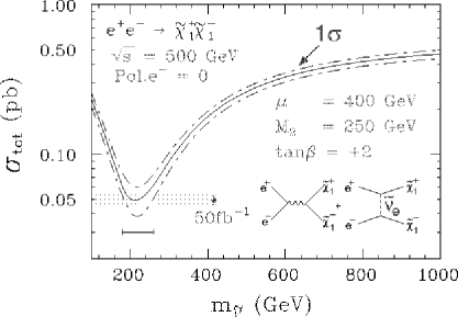
Figure 3.15: Lighter chargino pair production cross section as a function of $m_{\tilde{\nu}_{e}}$. The dot-dashed curves indicate the 1-$\sigma$ bound from the global fit (see the text).

We can see that the total cross section measurement constrains the sneutrino mass fairly well. Using this and the following model-independent inequality

$$\begin{array}[]{lll}m_{\tilde{e}^{\pm}_{L}}^{2}\leq m_{\tilde{\nu}_{e}}^{2}+0.77m_{Z}^{2},\end{array}$$ (3.13)

we can set an upper limit on the left-handed selectron mass. We can thus go and look for the left-handed selectron in $e^{+}e^{-}_{R}\to\tilde{e}^{+}_{L}\tilde{e}^{-}_{R}$.

3.3.4 $\bf\tilde{\it e}^{\pm}_{\it L}$ Study

$\bf\tilde{\it e}^{\pm}_{\it L}$ Signature

The associate production of $\tilde{e}_{L}$ with $\tilde{e}_{R}$ proceeds via $t$-channel exchange of neutralinos, to which only the $\tilde{B}$ components contribute. The decay of the left-handed slepton may be a little complicated, since they tend to decay in cascade as the scalar mass becomes heavier. Nevertheless, the branching fraction for the direct two-body decay into the LSP: $\tilde{l}_{L}^{\pm}\to l^{\pm}\tilde{\chi}_{1}^{0}$ usually exceeds $10~{}\%$. For our parameter set, the $\tilde{l}_{L}^{\pm}\to l^{\pm}\tilde{\chi}_{1}^{0}$ decay is actually dominant. The signal for this process is therefore an acoplanar $e^{+}e^{-}$ pair. When we use the right-handed electron beam to suppress standard-model backgrounds, the major background is our previous signal: $e^{+}e^{-}_{R}\to\tilde{e}^{+}_{R}\tilde{e}^{-}_{R}$. Notice that the use of the right-handed electron beam selects the $e^{+}$ in the final state as a carrier of the $\tilde{e}_{L}$ information. Fig. 3.16 plots the final-state electron energy against that of the positron, clearly demonstrating this fact.

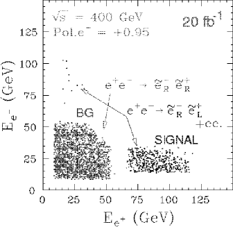
Figure 3.16: Distribution of final-state electron energy against that of the positron for $e^{+}e^{-}_{R}\to\tilde{e}^{+}_{L}\tilde{e}^{-}_{R}$ (signal) and $\tilde{e}^{+}_{R}\tilde{e}^{-}_{R}$ (background) at $\sqrt{s}=400~{}{\rm GeV}$ with an integrated luminosity of $20~{}{\rm fb}^{-1}$.

Mass Determination

Projecting Fig. 3.16 to the $E_{e^{+}}$ axis, we obtain the distribution shown in Fig. 3.17-a), from which we can extract the sparticle masses as before.

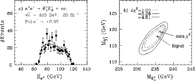
Figure 3.17: (a) Energy distribution of positrons from $\tilde{e}^{+}_{L}$ decays for the same Monte Carlo parameters as with Fig.3.16. The solid line corresponds to the best fit curve, letting $m_{\tilde{e}_{L}}$ and $m_{\tilde{\chi}^{0}_{1}}$ move freely. (b) Contours in the $m_{\tilde{e}_{L}}$-$m_{\tilde{\chi}^{0}_{1}}$ plane obtained from the fit to the energy distribution.

The contours from a 2-parameter fit are shown in Fig. 3.17-b), which tells us that we can determine the left-handed selectron mass to an accuracy better than $1~{}\%$ with $20~{}{\rm fb}^{-1}$.

Test of Left-Right Universality of Scalar Masses

Knowing both the right-handed and left-handed selectron masses enables us to make another test of the universal scalar mass hypothesis. The squared mass difference of the right-handed (belonging to $\bf 5^{*}$) and left-handed (belonging to $\bf 10$) selectrons is related through the following scalar mass formula:

$$\begin{array}[]{lll}m_{\tilde{e}_{L}}^{2}-m_{\tilde{e}_{R}}^{2}=m_{0({\bf 5})}^{2}-m_{0({\bf 10})}^{2}+0.5M_{2}^{2}-0.04\cdot m_{Z}^{2}\cos 2\beta.\end{array}$$ (3.14)

The universal scalar mass hypothesis implies the representation independence ($m_{0({\bf 5})}=m_{0({\bf 10})})$, which can be tested as shown in Fig. 3.18: compare the $\Delta\chi^{2}=1$ contour with the prediction of the universal scalar mass hypothesis (dashed lines for $\tan\beta=0$ and $30$). Notice that the last term ($\tan\beta$-dependent term) of the above equation is small and only makes slight difference, allowing us a clean test of the representation independence.

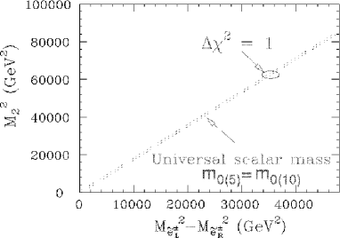
Figure 3.18: $\Delta\chi^{2}=1$ contour from the selectron mass measurements, compared with the prediction from the universal scalar mass hypothesis, indicated as dotted lines for $\tan\beta=0$ and $30$.

Once the GUT relation is confirmed and the universal scalar mass hypothesis is verified in the slepton sector, we can set, with confidence, the next target energy for $\tilde{q}$ pair production.

3.3.5 Study of $\bf\tilde{\it q}_{\it G}({\it G}\neq 3)$

Squark Signature

A squark may decay into a quark plus an LSP or into a quark plus a chargino or heavier neutralino, depending on the SUSY breaking parameters. In the former case, the signal for squark pair production is an acoplanar 2-jet final state, while in the latter case it is a final state consisting of two jets plus one or two $W/Z$ bosons from the cascade decays of the charginos or neutralinos, respectively. Potential backgrounds to this process thus include $e^{+}e^{-}\to W^{+}W^{-}$, $e^{\pm}\mathop{\nu_{e}}\limits^{\mbox{\scriptsize$(-)$}}W^{\mp}$, $\nu\bar{\nu}Z$, $\tilde{\chi}^{+}_{1}\tilde{\chi}^{-}_{1}$, and $\tilde{\chi}^{0}_{i}\tilde{\chi}^{0}_{j}$. Notice that the 2-jet systems in the final states of these background processes are all from $W^{(*)}/Z^{(*)}$’s, thereby having invariant masses smaller than $100~{}{\rm GeV}$. We can therefore very effectively eliminate them by requiring $m_{q\bar{q}}>100~{}{\rm GeV}$, together with usual acoplanar 2-jet selection criteria like $\not{\!{p}}_{T}>35~{}{\rm GeV}$, and $\theta_{A}>30^{\circ}$. We can thus use both $e^{-}_{L}$ and $e^{-}_{R}$ beams without suffering from these would-be serious backgrounds. It should also be emphasized that the chirality selection of the final-state squarks works better than the slepton case: $\sigma_{R}(\tilde{q}_{R}\bar{\tilde{q}}_{R}):\sigma_{R}(\tilde{q}_{L}\bar{\tilde{q}}_{L})\simeq\sigma_{L}(\tilde{q}_{L}\bar{\tilde{q}}_{L}):\sigma_{L}(\tilde{q}_{R}\bar{\tilde{q}}_{R})\simeq 9:1$, if $m_{\tilde{q}_{L}}\simeq m_{\tilde{q}_{R}}$. By controlling the electron beam polarization, we can thus select the chirality of the final-state squarks and, consequently, study their properties separately.

Mass Determination

Let us first consider the mass determination in the case of the direct decay. In this case, we can use the end-point method as with $\tilde{l}^{\pm}$ and $\tilde{\chi}^{\pm}_{1}$. There is, however, a better quantity called minimum squark mass ($m_{\tilde{q}}^{min}$)[33]. defined by

$$\begin{array}[]{lll}\left(m_{\tilde{q}}^{min}\right)^{2}=E_{beam}^{2}-|{\bf p}_{1}|^{2}_{max}=E_{beam}^{2}-|{\bf p}_{2}|^{2}-|{\bf p}_{3}|^{2}+2|{\bf p}_{2}||{\bf p}_{3}|\cos(\delta+\gamma),\end{array}$$ (3.15)

where the momenta and angles are defined in Fig. 3.20.

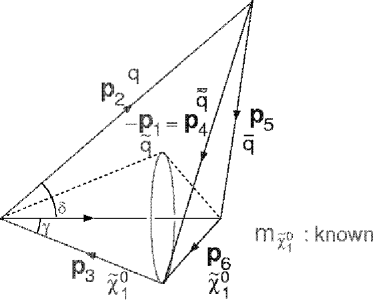
Figure 3.19: Definitions of the momenta and angles used to define the minimum squark mass. The LSP mass is assumed to be known precisely.

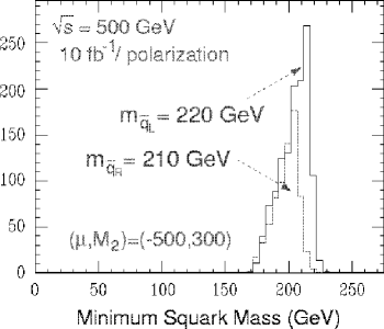
Figure 3.20: Expected $m_{\tilde{q}}^{min}$ distributions for left- and right-handed squarks cited from Ref.[33].

Notice that the two angles $\delta$ and $\gamma$ and the magnitude of the LSP momentum are calculable, provided that the LSP mass is known. Notice also that $m_{\tilde{q}}^{min}$ makes use of the information contained in the relative configuration of the final-state $q$ and $\bar{q}$ unlike in the end-point method. Fig. 3.20 shows an example of expected $m_{\tilde{q}}^{min}$ distributions for parameters shown in the figure. We can see that the Jacobian peaks are good measures of the squark masses and allow their precision measurements: $\Delta m_{\tilde{q}}\simeq 1~{}{\rm GeV}$ at the $95~{}\%$ confidence level. The effects of the radiative corrections to production and decay as well as the effects of the ISR have been studied separately[34] and found to be harmless: the peak of the $m_{\tilde{q}}^{min}$ distribution is essentially unaffected as shown in Fig. 3.21 and still allows us to measure the squark mass to a percent level with $50~{}{\rm fb}^{-1}$.

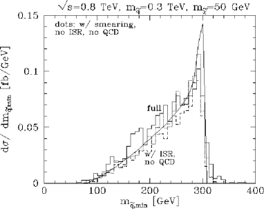
Figure 3.21: Accuracy of determination of the squark mass using the $m_{\tilde{q}}^{min}$ estimator. The input squark mass is 300 GeV and Monte Carlo data were generated at $\sqrt{s}=0.8$ TeV and correspond to $50~{}{\rm fb}^{-1}$

If cascade decays dominate the direct decay, we select final-states with two jets plus leptons and pretend to be blind to the leptons. Notice that these leptons are end-products of the chargino ($\tilde{\chi}^{\pm}_{1}$) or heavier neutralino ($\tilde{\chi}^{0}_{2}$), whose masses are almost degenerate and presumably known from the earlier measurements. We can thus change the role of the LSP in the direct decay case by that of the chargino or second neutralino, by ignoring the final-state leptons. In this way, we can again calculate the minimum squark mass for each event and carry out the squark mass measurement at a $1~{}\%$ level, provided that $m_{\tilde{\chi}^{\pm}_{1}}$ and $m_{\tilde{\chi}^{0}_{1}}$ are known.

3.3.6 Study of Third Generation Sleptons

For the first and second generation, we could ignore the left-right mixing. This is due to the fact that the off-diagonal element of the mass matrix:

$${\cal M}^{2}_{\tilde{f}}=\left(\begin{array}[]{cc}m_{\tilde{f}_{L}}^{2}&-m_{f}(A_{f}+\mu\tan\beta)\cr-m_{f}(A_{f}+\mu\tan\beta)&m_{\tilde{f}_{R}}^{2}\end{array}\right),$$ (3.16)

which is responsible for the left-right mixing is proportional to the corresponding fermion mass. For the third generation, since the tau mass ($m_{\tau}$) is much heavier than the other leptons, this off-diagonal element can be substantial, if the soft SUSY-breaking trilinear scalar coupling ($A_{\tau}$) or $\mu\tan\beta$ or both are large. The mass eigen states therefore become mixtures of $\tilde{\tau}_{L}$ and $\tilde{\tau}_{R}$:

$$\pmatrix{\tilde{\tau}_{1}\cr\tilde{\tau}_{2}}=\pmatrix{\cos\theta_{\tau}&\sin\theta_{\tau}\cr-\sin\theta_{\tau}&\cos\theta_{\tau}}\pmatrix{\tilde{\tau}_{L}\cr\tilde{\tau}_{R}},$$ (3.17)

where $m_{\tilde{\tau}_{1}}<m_{\tilde{\tau}_{2}}$ by definition.

Note also that the $\tau$ lepton has a Yukawa coupling:

$$Y_{\tau}=-gm_{\tau}/(\sqrt{2}m_{W}\cos\beta),$$

which becomes non-negligible for a large $\tan\beta$. The correction to the diagonal elements is proportional to $Y_{\tau}^{2}\log(M_{GUT}/M_{W})$ and makes $m_{\tilde{\tau}_{L(R)}}$ smaller than those of the first and second generations. If $\tan\beta$ is large, $\mu\tan\beta$ that controls the off-diagonal element becomes substantial and consequently lowers the lighter stau mass further. In SUGRA, we thus expect that the lighter stau is lighter than the other sleptons.

Conversely, once the masses of the two staus, their mixing angle, and the tau Yukawa coupling are determined, we can calculate $m_{\tilde{\tau}_{L(R)}}$ thereby testing the prediction of SUGRA. It has been pointed out that the determination of $m_{\tilde{\tau}_{L(R)}}$ is crucial for testing grand unified theories: in GUTs a heavy colored Higgs boson with a mass of $O(M_{GUT})$ couples to the stau leptons via strong Yukawa interactions and further reduces $m_{\tilde{\tau}_{L,R}}$.

In this way, the stau can be the first slepton to be discovered at the JLC and, once it is found, its detailed studies may provide us an evidence of grand unification at high scale.

Stau Signature

The lighter stau $\tilde{\tau}_{1}$ decays into a chargino ($\chi^{+}_{i}$) and a tau neutrino ($\nu_{\tau}$) or into a neutralino ($\chi^{0}_{i}$) and a tau ($\tau$). The latter decay mode leaves an acoplanar tau pair in the final state and provides a signature of the stau production. In particular when $\tilde{\tau}_{1}$ is the lightest charged SUSY particle, it decays into the lightest neutralino and a tau. The taus in the final state further decay into $e(\mu)\bar{\nu}_{e(\mu)}\nu_{\tau}$, $\pi\nu_{\tau}$, $\rho\nu_{\tau}\rightarrow\pi^{+}\pi^{0}\nu_{\tau}$, etc. Consequently, the stau pair production results in an acoplanar event consisting of a pair of leptons or low multiplicity hadron jets. The most serious background in the search of the stau pair production is the two-photon process: $e^{+}e^{-}\rightarrow e^{+}e^{-}\tau^{+}\tau^{-}$, which mimics the stau pair production when the final-state $e^{+}$ and $e^{-}$ escape from detection into the beam-pipe. Note that for this background, the missing transverse momentum ($P_{T}$) cut is not that effective, because of the neutrinos from the tau decays always carrying away significant fraction of $P_{T}$. Simultaneous cuts on the polar angles of the jets, $\cos\theta_{jet}$, and the acoplanarity, $\theta_{acop}$, are effective but still not enough to reduce the huge background for signal events with a missing $P_{T}$ that is similar to the $P_{T}$’s carried away by the escaping $e^{+}$ and $e^{-}$. It is essential to be able to veto low angle electrons and positrons to reduce the two-photon background. We will return to this point later.

Polarization Measurements

Since the stau decays in cascade, its analysis is complicated. Its detailed study, however, provides us with another handle to uncover the nature of the LSP. Namely, we can study the polarization of the tau leptons by measuring the energy distribution of the tau’s decay products[35]. Fig. 3.22 plots the distribution of $E_{\pi^{\pm}}/E_{\rho}$ for the cascade decay: $\tilde{\tau}_{1}\rightarrow\tau\tilde{\chi}^{0}_{1}$ followed by $\tau\rightarrow\rho\nu_{\tau}$, $\rho\rightarrow\pi^{\pm}\pi^{0}$, when the intermediate tau has the right-handed or left-handed polarization. We can see that the right-handed tau tends to give most of its energy to one of the $\pi^{+}$, $\pi^{0}$, while the left-handed tau tends to equally distribute its energy to both of them. Given $10^{4}$ stau pairs, the Monte Carlo simulations tells us that the tau polarization can be measured to an accuracy of $8\%$.

         

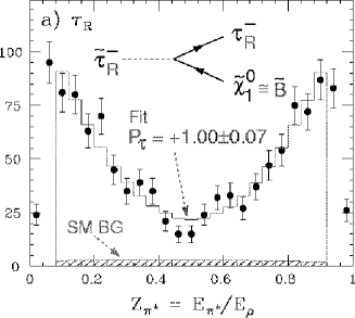
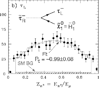
Figure 3.22: $z_{c}=E_{\pi^{\pm}}/E_{jet}$ distribution of the selected candidates of the cascade decay: $\tilde{\tau}_{1}\rightarrow\tau\tilde{\chi}^{0}_{1}$ followed by $\tau\rightarrow\rho\nu$ for $10^{4}$ Monte Carlo stau pair events. The histograms are the results of the fits to determine the tau polarization.

The tau polarization provides a very important piece of information for the determination of the stau’s Yukawa coupling. Let us now consider the $\tilde{\tau}_{R(L)}$- $\chi^{0}_{1}$-$\tau$ coupling which is relevant to the stau decay. The neutralinos ($\tilde{\chi}^{0}_{1}$, $\tilde{\chi}^{0}_{2}$, $\tilde{\chi}^{0}_{3}$, $\tilde{\chi}^{0}_{4}$) are the mixtures of the bino ($\tilde{B}^{0}$), the wino ($\tilde{W}^{0}_{3}$), and the two higgsinos ($\tilde{H}^{0}_{1}$, $\tilde{H}^{0}_{2}$), whose mass matrix is given by

$${\cal M}_{N} = \left(\begin{array}[]{cccc}M_{1}&0&-m_{Z}\sin\theta_{W}\cos\beta&m_{Z}\sin\theta_{W}\sin\beta\\ 0&M_{2}&m_{Z}\cos\theta_{W}\cos\beta&-m_{Z}\cos\theta_{W}\sin\beta\\ -m_{Z}\sin\theta_{W}\cos\beta&m_{Z}\cos\theta_{W}\cos\beta&0&-\mu\\ m_{Z}\sin\theta_{W}\sin\beta&-m_{Z}\cos\theta_{W}\sin\beta&-\mu&0\end{array}\right)$$ (3.22)

and its mass eigen states can be expressed in the form:

$$\tilde{\chi}^{0}_{i}=N_{i1}\tilde{B}^{0}+N_{i2}\tilde{W}^{3}+N_{i3}\tilde{H}^{0}_{1}+N_{i4}\tilde{H}^{0}_{2}.$$

Fig. 3.23 illustrates the right-handed stau’s interaction with the bino and higgsino components. Notice that the interaction differs not only in its strength but also in the resultant polarization of the final-state tau.

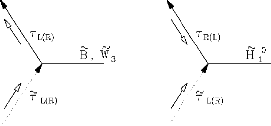
Figure 3.23: Feynmann diagarams for $\tilde{\tau}_{R}$ decaying into a tau and a bino ($\tilde{B}^{0}$) or a higgsino ($\tilde{H}^{0}_{1}$). The white arrows indicate chirality flow.

In general, interaction of matter fermions with gauge bosons preserves chirality, while that with the Higgs bosons flips it. By supersymmetry, therefore, $\tilde{\tau}_{R(L)}$ interacts with a gaugino (higgsino) and turns into a $\tau_{R(L)}$($\tau_{L(R)}$). The polarization of the daughter tau is determined by the neutralino mixing angles, $N_{ij}$, and the stau mixing angle, $\theta_{\tilde{\tau}}$, and, in the limit that the neutrarino is a pure bino and the stau is a weak eigen state, i.e. either $\tilde{\tau}_{R}$ or $\tilde{\tau}_{L}$, is expressed as

$$P_{\tau}\left(\tilde{\tau}_{1}\rightarrow\tilde{B}\tau\right) = \frac{4\sin^{2}\theta_{\tilde{\tau}}-\cos^{2}\theta_{\tilde{\tau}}}{4\sin^{2}\theta_{\tilde{\tau}}+\cos^{2}\theta_{\tilde{\tau}}}$$

$$P_{\tau}\left(\tilde{\tau}_{R}\rightarrow\tilde{\chi}^{0}_{1}\tau\right) = \frac{\left(\sqrt{2}N_{11}\tan\theta_{W}\right)^{2}-\left(Y_{\tau}N_{13}\right)^{2}}{\left(\sqrt{2}N_{11}\tan\theta_{W}\right)^{2}+\left(Y_{\tau}N_{13}\right)^{2}}$$

$$P_{\tau}\left(\tilde{\tau}_{L}\rightarrow\tilde{\chi}^{0}_{1}\tau\right) = \frac{\left(\sqrt{2}Y_{\tau}N_{13}\right)^{2}-g^{2}\left(N_{12}+N_{11}\tan\theta_{W}\right)^{2}}{\left(\sqrt{2}Y_{\tau}N_{13}\right)^{2}+g^{2}\left(N_{12}+N_{11}\tan\theta_{W}\right)^{2}}.$$

Notice that, unless the neutralino is a pure bino, the polarization depends on the Yukawa coupling. We shall discuss later how this can be exploited to determine the Yukawa coupling, when the neutralino and stau mixing angles can be constrained.

Mass Determination

The masses of the first and second generation sleptons and the lightest neutralino could be determined by measuring the end points of the square-shaped energy distribution of the daughter leptons from the slepton decays. For the stau, however, since the daughter tau from its decay further decays into a neutrino and hadrons, the mass determination must rely not merely on the end points but the shape of the distribution of the energy of the decay products from the tau decay. Fig. 3.24 shows the energy distributions of the final-state hadrons for the $\tau\rightarrow\nu_{\tau}+\pi^{-}/\rho^{-}$ decays. The higher end point of the distribution is equal to that of the tau energy distribution, while the peak of the energy distribution of the $\rho$’s corresponds to the lower limit of the tau energy distribution. If we can determine these two values, we can thus obtain the stau and the neutralino masses. The energy distribution depends on the tau polarization, but it can be measured as explained above.

         

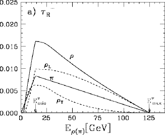
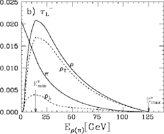
Figure 3.24: Energy distributions of $\rho(\pi)$’s from $\tilde{\tau}\rightarrow\tau_{L(R)}$ $\rightarrow\rho(\pi)$ decays for $m_{\tilde{\tau}}=150$ GeV, $m_{\tilde{\chi}^{0}_{1}}=100$ GeV, and $\sqrt{s}=500$ GeV. $E^{\tau}_{max}$ and $E^{\tau}_{min}$ are the upper and lower limits of the tau energy.

Fig.3.25-a)

         

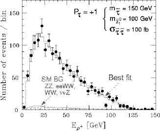
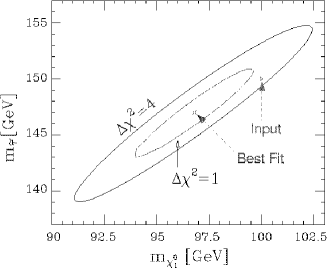
Figure 3.25: a) energy distribution of the final-state hadrons selected as $\rho$’s from stau decays shown together with the best fit, when $10^{4}$ $\tilde{\tau}_{1}$ stau pairs are produced and decay in the $\tilde{\chi}^{0}_{1}\tau_{R}$ mode. b) $\Delta\chi^{2}=1,4$ contour in the $m_{\tilde{\chi}^{0}_{1}}$-$m_{\tilde{\tau}_{1}}$ plane.

shows the tau energy distribution for Monte Carlo data with background events, when $10^{4}$ stau pairs are produced. The expected resolution for the stau mass is 2.6%, while that for the $\tilde{\chi}^{0}_{1}$ mass is 2.8%. These accuracies are worse than what we expect for the first and second generation sleptons, which is due to the fact that the tau energy end points are more difficult to measure. Note that, if the other sleptons are already found, we can use the $\chi^{0}_{1}$ mass from the end point measurements for them to improve the measurement.

Determination of Mixing Angle

Once the cross section and the stau mass are measured, we can determine the stau mixing angle. Fig.3.26 shows the expected contour of $\Delta\chi^{2}=1,4$ in the $m_{\tilde{\tau}_{1}}$-$\sin\theta_{\tilde{\tau}}$ plane for $m_{\tilde{\tau}}=150$ GeV and $m_{\tilde{\chi}^{0}_{1}}=100$ GeV, when the production cross section is 50 fb (corresponding to $\sin\theta_{\tilde{\tau}}=0.7526$) and an integrated luminosity of 100 ${\rm fb}^{-1}$ is accumulated at $\sqrt{s}=500$ GeV. In this case, $\sin\theta_{\tilde{\tau}}$ can be determined to 6.5%.

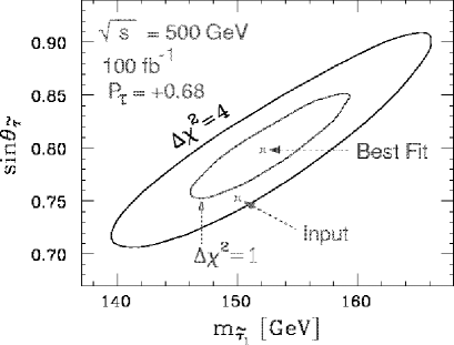
Figure 3.26: The $\Delta\chi^{2}=1,4$ contour in the $m_{\tilde{\tau}_{1}}$-$\sin\theta_{\tilde{\tau}}$ plane obtained from a fit of 5000 Monte Carlo stau pair events generated at $\sqrt{s}=500$ GeV for $m_{\tilde{\tau}}=150$ GeV, $m_{\tilde{\chi}^{0}_{1}}=100$ GeV, $P_{\tau}=0.6788$, and $\sin\theta_{\tilde{\tau}}=0.7526$. The Monte Carlo statistics is $\int{\cal L}dt=100{\rm fb}^{-1}$ equivalent. The tau polarization corresponds to the case in which the stau decays into a tau and a bino.

Determination of Yukawa Coupling

As mentioned above, the tau polarization carries information on the stau’s Yukawa coupling. In order to extract the information on the stau’s Yukawa coupling, we need to determine the mixing angles of the stau and the neutralino. The stau’s mixing angle can be determined by measuring the production cross section. Combining the information from the productions of the other sleptons, we can further decide the neutralino mixing, and consequently obtain the information on the stau’s Yukawa coupling.

Fig. 3.27 shows the tau polarization in the $M_{1}$-$\tan\beta$ plane, when the $\tilde{\tau}_{R}$ decays into a tau and a 100 GeV neutralino.

  

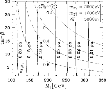
Figure 3.27: The neutralino-mixing dependence of the tau polarization in the $\tilde{\tau}_{1}\rightarrow\tau\tilde{\chi}^{0}_{1}$ decay. The neutralino mixing angle is determined by $(M_{1},M_{2},\mu,\tan\beta)$ in general. If we assume the GUT relation, $M_{1}=5/3\cdot\tan^{2}\theta_{W}M_{2}$, and $m_{\tilde{\chi}^{0}_{1}}=100$ GeV, we can eliminate two of the four parameters. The tau polarization is thus shown in the $M_{1}-\tan\beta$ plane.

We assumed the GUT relation for $M_{1}$ and $M_{2}$. Notice that the neutralino mass matrix is completely determined by $M_{1}$, $M_{2}$, $\mu$, and $\tan\beta$. Once the neutralino mass is given, therefore, the neutralino properties are completely determined by the two parameters.

Fig. 3.28, on the other hand, demonstrates how the tau polarization and the selectron and stau cross section measurements constrain $\tan\beta$ in the $M_{1}$-$\tan\beta$ plane, where we assumed that the measurement errors are dominated by statistical ones and that the GUT relation between $M_{1}$ and $M_{2}$ holds .

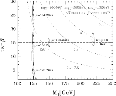
Figure 3.28: The $1\sigma$ error contours in the $M_{1}$-$\tan\beta$ plane expected from the measurements of the selectron and stau productions. The contours are plotted for $m_{\tilde{\tau}_{1}}=150$ GeV, $\sin\theta_{\tilde{\tau}}=1$ ($\tilde{\tau}_{1}=\tilde{\tau}_{R}$), $m_{\tilde{\chi}^{0}_{1}}=100$ GeV($\mu>0$), and $m_{\tilde{e}_{R}}=200$ GeV.

The points in the figure indicate the input model parameter sets and the curves surrounding them are the expected $\Delta\chi^{2}=1$ contours. The neutralino, stau, and selectron masses are fixed at 100 GeV, 150 GeV, and 200 GeV, respectively. Notice that $\tan\beta$ determination becomes less accurate as $M_{1}$ decreases. This is because $\tilde{\chi}^{0}_{1}$ becomes more and more $\tilde{B}$-like, as $M_{1}$ approaches $m_{\tilde{\chi}^{0}_{1}}$, and consequently loses the $\tan\beta$ dependence of the tau polarization. On the other hand, in the large $M_{1}$ and $\tan\beta$ region, we can determine $\tan\beta$ reasonably well.

There are other possibilities to determine $\tan\beta$. The $\tan\beta$ measurement using the stau production is, however, particularly useful when $\tan\beta>10$. On the other hand, the determinations using the $\tilde{e}_{L}$-$\tilde{\nu}_{L}$ mass difference or the forward-backward asymmetry of the chargino pair production are very effective for $\tan\beta\hbox{ \raise 3.0pt\hbox to0.0pt{$<$}\raise-3.0pt\hbox{$\sim$} }5$. The Higgs production is also effective for $\tan\beta\hbox{ \raise 3.0pt\hbox to0.0pt{$<$}\raise-3.0pt\hbox{$\sim$} }10$ (See Fig.3.29).

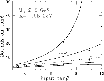
Figure 3.29: The constraint on $\tan\beta$ from the measurement of the forward-backward asymmetry of the chargino production for $M_{2}=210$ GeV, $\mu=-195$ GeV, and $m_{\tilde{\nu}_{e}}=500$ GeV. The error on the two chargino masses is assumed to be common and 2%.

3.4 Other Scenarios

Up to now we have been concentrating our attention on typical SUGRA scenarios. We now turn to other scenarios and examine expected complications and possible ways out. We will first study a particular case where the lighter chargino decays into $\tilde{\tau}_{1}+\nu_{\tau}$ and therefore the end-point method we used for the $\tilde{\chi}_{1}^{\pm}\to W^{\pm}\tilde{\chi}_{1}^{0}$ decay is not applicable. Effects of possible $CP$ phases will be described after this. We then move on to examine other SUSY breaking schemes: Gauge Mediated Supersymmetry Breaking (GMSB) and Anomaly Mediated Supersymmetry Breaking (AMSB), which will be followed by discussions on $R$-parity violation.

3.4.1 Chargino Decaying into Stau plus Neutrino

As we have seen above, if $\tan\beta$ is large, it is quite possible that the stau is the first SUSY particle to be discovered at JLC. If the mass hierarchy (expected at large $\tan\beta$ in (M)SUGRA scenario as well) is such that $m_{\tilde{l}}>m_{\tilde{\chi}_{1}^{\pm}}>m_{\tilde{\tau}_{1}}>m_{\tilde{\chi}_{1}^{0}}$, then the lighter chargino almost 100 % decays into $\tilde{\tau}_{1}+\nu_{\tau}$, through the left-handed component due to the stau’s left-right mixing. The signature of the chargino pair production becomes a pair of acoplanar tau leptons. The background processes thus include the former signal process: $e^{+}e^{-}\to\tilde{\tau}_{1}^{+}\tilde{\tau}_{1}^{-}$, and the standard model ones: $ee\tau\tau$, $WW$, and $ZZ$. Nevertheless, it has been shown that we can determine the chargino mass by measuring the $\tau$-jet energy. In this scenario, the chargino mass determination based on the end-point measurement of the daughter $W$’s from the $\tilde{\chi}_{1}^{\pm}\to W^{\pm}\tilde{\chi}_{1}^{0}$ decay will be useless. For the mass hierarchy given above, however, we can assume that $m_{{\tilde{\tau}}_{1}}$ and $m_{\tilde{\chi}_{1}^{0}}$ to be known from the studies of $\tilde{\tau}_{1}^{+}\tilde{\tau}_{1}^{-}$ production. Using the $E_{jet}$ distribution ($\tau$ is detected as a low multiplicity jet), therefore, we can still determine the chargino mass: for an integrated luminosity of $200~{}{\rm fb}^{-1}$, with inputs $m_{\tilde{\chi}_{1}^{+}}$ = 172.5 GeV, $m_{\tilde{\tau}_{1}}$ = 152.7 GeV, and $m_{\tilde{\chi}_{1}^{0}}$ = 86.8 GeV, the fit to the $E_{jet}$ distribution yielded $m_{\tilde{\chi}_{1}^{+}}=171.8\pm 0.5$ GeV (see Fig. 3.30-(a) for the $\Delta\chi^{2}$ curve).

         

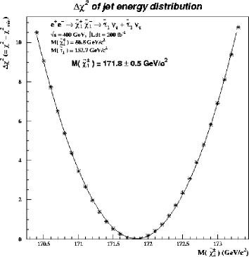
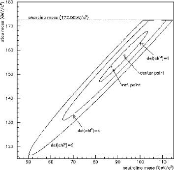
Figure 3.30: (a) $\Delta\chi^{2}$ for the energy distribution of the $\tau$ jets from $\tilde{\chi}_{1}^{\pm}\to\tilde{\tau}_{1}^{\pm}\mathop{\nu_{\tau}}\limits^{\mbox{\scriptsize$(-)$}}\to\tau^{\pm}\tilde{\chi}_{1}^{0}\mathop{\nu_{\tau}}\limits^{\mbox{\scriptsize$(-)$}}$, (b) contours of the $\Delta\chi^{2}$, when the stau and the neutralino masses are changed. Input masses are $m_{\tilde{\chi}_{1}^{+}}$ = 172.5 GeV, $m_{\tilde{\tau}_{1}}$ = 152.7 GeV, and $m_{\tilde{\chi}_{1}^{0}}$ = 86.8 GeV. An integrated luminosity of $200~{}{\rm fb}^{-1}$ is assumed.

This value is obtained, assuming that the errors on the stau and the LSP masses are negligible. In order to estimate their effects on the chargino mass determination, their $\chi^{2}$ contribution to the $E_{jet}$ fit has been estimated, which is shown in Fig. 3.30-(b). which is shown in Fig. 3.30-(b). If the error on these masses are less than 3 GeV, as expected from Fig. 3.25, the effect will not be a problem.

3.4.2 $\bf CP$ Violating Phases

As already exemplified in the previous section (3.3.3), the new mass parameters introduced in association with supersymmetry contain $CP$ phases that cannot be eliminated by field redefinitions. We have not yet examined their effects in any detail and that is what we will turn our attention to here. Firstly, it should be noted that the $CP$ phases can modify not only the couplings but also the sparticle mass spectrum significantly[36]. Secondly, although there are potentially many $CP$ violating phases in the full MSSM Lagrangian, it is known that only two $CP$-odd rephase-invariant phases:

$$\mu=\left|\mu\right|\exp^{i\phi_{\mu}}~{}~{}~{}~{}~{}\mbox{and}~{}~{}~{}~{}~{}~{}M_{1}=\left|M_{1}\right|\exp^{i\phi_{1}},$$

stemming from the chargino and neutralino mass matrices, take part in the chargino and neutralino production processes.

$\bf e^{+}e^{-}\to\tilde{\chi}_{1}^{0}\tilde{\chi}_{2}^{0}\to\tilde{\chi}_{1}^{0}\tilde{\chi}_{1}^{0}l^{+}l^{-}$

The good place, where we can study the effects of the $CP$-violating phases, is the following associated neutralino production process: $e^{+}e^{-}\to\tilde{\chi}_{1}^{0}\tilde{\chi}_{2}^{0}$, followed by $\tilde{\chi}_{2}^{0}\to\tilde{\chi}_{1}^{0}l^{+}l^{-}$[37, 38], since it is likely that this is the first process to access the gaugino sector, and that the final-state leptons allow us to construct clean and useful observables for the study of the $CP$ phases. First such an observable is the dilepton invariant mass ($m_{ll}$). It is note worthy that the distribution shape of this observable is independent of the production mechanism of the decaying neutralino, which is because the invariant mass does not involve any angular variables describing the decays so that the polarization of the decaying neutralino is irrelevant. In Ref.[38], two scenarios (${\cal S}1$ and ${\cal S}2$) are considered that satisfy the electron EDM constraints:

$$\begin{array}[]{lllll}{\cal S}1:&{}&M_{2}=100~{}{\rm GeV},&\left|\mu\right|=200~{}{\rm GeV},&m_{\tilde{e}}=10~{}{\rm TeV}\cr{\cal S}2:&{}&M_{2}=100~{}{\rm GeV},&\left|\mu\right|=700~{}{\rm GeV},&m_{\tilde{e}}=200~{}{\rm GeV}.\end{array}$$

Figs.3.31-a) and -b) show the invariant mass distributions for the two cases.

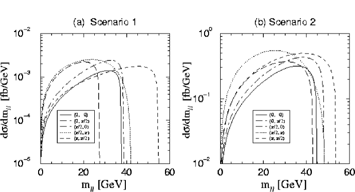
Figure 3.31: Dilepton invariant mass distributions for the process: $e^{+}e^{-}\to\tilde{\chi}_{1}^{0}\tilde{\chi}_{2}^{0}\to\tilde{\chi}_{1}^{0}\tilde{\chi}_{1}^{0}l^{+}l^{-}$ in (a) scenario ${\cal S}1$ and (b) ${\cal S}2$ for five combinations of the values of two $CP$ phases: $\phi_{\mu}$ and $\phi_{1}$. [38].

We can see that the $m_{ll}$ distribution is sensitive to the $CP$ phases.

The final-state lepton angular distribution is also known to be useful. Unlike the dilepton invariant mass this variable is crucially dependent on the production-decay spin correlations, and its distribution shape sensitively reflects the slepton mass and the neutralino mixing[37].

The two observables discussed above are $CP$-even and only indirectly depends on the $CP$ phases. It is possible, however, to construct a $T$-odd, thus $CP$-odd, observable:

$${\cal O}_{T}={\bf p}_{e}\cdot({\bf p}_{l^{-}}\times{\bf p}_{l^{+}}),$$

whose expectation value can be sizable in scenario ${\cal S}2$, thereby directly signaling the $CP$ phases at work[38]. Fig. 3.32 is an expected exclusion plot for the $CP$ phases from the measurement of ${\cal O}_{T}$ at $\sqrt{s}=500~{}{\rm GeV}$ with an integrated luminosity of $200~{}{\rm fb}^{-1}$.

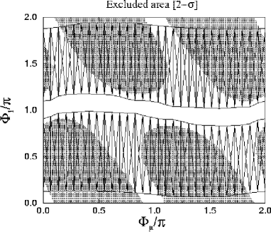
Figure 3.32: Expected $95\%$-confidence-level excluded regions of the $\phi_{\mu}$-$\phi_{1}$ plane by the EDM constraints (shaded) and by the ${\cal O}_{T}$ measurement at $\sqrt{s}=500~{}{\rm GeV}$ with $200~{}{\rm fb}^{-1}$.

One can see that the ${\cal O}_{T}$ measurement is complementary to the EDM measurement shown as shaded regions.

$\bf e^{+}e^{-}\to\tilde{t}_{1}\tilde{t}_{1}^{*}h$

In the light of possible $CP$ phases that may appear in the scalar sector, $e^{+}e^{-}\to\tilde{t}_{1}\tilde{t}_{1}^{*}h$ is interesting, since the stop can be light enough to make this process useful already at $\sqrt{s}=500~{}{\rm GeV}$. The $CP$ violating phases in $A_{t}$ and $\mu$ affects not only the masses and the mixings of the stops and the Higgs bosons but also the $\tilde{t}\tilde{t}^{*}h$ coupling, which has been studied in Ref.[39]. In order to satisfy the neutron electric dipole constraints as well as cosmological ones[40], the following conditions are imposed in the study: i) Arg($\mu)<10^{-2}$, ii) $m_{\tilde{g}}>400$ GeV, iii) $|A_{e}|,|A_{u,c}|,|A_{d,e}|<10^{-3}|\mu|$, and iv) maximal mixing in the stop sector $|A_{t}|=|\mu\cot\beta|$.

      

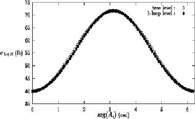
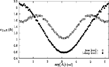
Figure 3.33: Effect of loop corrections on $\sigma(\tilde{t}_{1}\tilde{t}_{1}^{*})$ (left) and $\sigma(\tilde{t}_{1}\tilde{t}_{1}^{*}h)$ (right) as a function of Arg$(A_{t})$ for $\sqrt{s}=500$ GeV, $\mu=500$ GeV, $|A_{t}|=250$ GeV, $M_{A}\simeq 194$ GeV, $\tan\beta=2$, and $M_{\rm SUSY}=500$ GeV[39].

Fig. 3.33 shows $\sigma_{L+R}(e^{+}e^{-}\to\tilde{t}_{1}\tilde{t}_{1}^{*})$ and $\sigma_{L+R}(e^{+}e^{-}\to\tilde{t}_{1}\tilde{t}_{1}^{*}h)$ in the left and the right panels, respectively. We see that though the loop effects are minimal in $\tilde{t}_{1}\tilde{t}_{1}^{*}$ production, the dependence on Arg($A_{t}$) is quite strong. This strong dependency comes from the strong dependence of the stop mass $m_{\tilde{t}_{1}}$ on Arg($A_{t}$). On the other hand for $e^{+}e^{-}\to\tilde{t}_{1}\tilde{t}_{1}^{*}h$ the cross sections are rather small (a few fb level) but loop effects are substantial and can be as much as 100 %. This is because the light Higgs boson mass can be strongly affected by loop corrections with the complex trilinear coupling $A_{t}$. though the neutral Higgs boson mixing can hardly be changed significantly. It is in principle possible to extract $|A_{t}|$, Arg$(A_{t})$ by combining the measurements of these cross-sections with the knowledge of higgs masses[39].

3.4.3 Gauge Mediated Supersymmetry Breaking

As a result of the super-Higgs mechanism, the gravitino acquires a SUSY-breaking mass:

$$m_{\tilde{G}}=\frac{F}{\sqrt{3}M_{Pl}}\simeq\left(\frac{\sqrt{F}}{100~{}{\rm TeV}}\right){\rm eV},$$

where $M_{Pl}$ is the reduced Planck mass given by $M_{Pl}=(8\pi G_{N})^{-1/2}$. As already mentioned in Section 3.2, the GMSB thus predicts a very light gravitino mass for the theoretically allowed range of the SUSY breaking scale: $10<\sqrt{F}<10^{4}~{}{\rm TeV}$ shown in Table 3.1. In the GMSB models, therefore, the LSP is always the gravitino. Since the longitudinal component of the now massive gravitino, being the goldstino originally, has an effective coupling with the NLSP that is proportional to

$$\left(\frac{E_{\tilde{G}}}{M_{Pl}}\right).\left(\frac{E_{\tilde{G}}}{m_{\tilde{G}}}\right)\simeq\left(\frac{E_{\tilde{G}}^{2}}{F}\right)\simeq\left(\frac{M_{NLSP}}{\sqrt{F}}\right)^{2},$$

which can be much larger than one would expect for gravitational interaction This makes the NLSP decay into the gravitino relevant to collider phenomenology. The decay length is given by

$$L=c\tau\beta\gamma\propto\frac{1}{(M_{NLSP})^{5}}(\sqrt{F})^{4}$$

and depends on the model parameters. Since $\sqrt{F}$ spans a very wide range (see Table 3.1), so does the expected decay length:

$$10^{-4}<L<10^{5}~{}{\rm cm}.$$

Since the GMSB models preserve the GUT relation among the gauginos and usually predict light sleptons lighter as compared with the SUGRA models, the NLSP will be $\tilde{\chi}_{1}^{0}$, or $\tilde{\tau}_{1}$, or $\tilde{l}_{R}(l\neq\tau)$, depending on the model parameters. There are thus logically nine cases to be considered:

$$\pmatrix{NLSP=\tilde{\chi}^{0}_{1}\cr NLSP=\tilde{\tau}_{1}\cr NLSP=\tilde{l}_{R}}\otimes\pmatrix{L\ll R\cr L\hbox{ \raise 3.0pt\hbox to0.0pt{$<$}\raise-3.0pt\hbox{$\sim$} }R\cr L\gg R}$$ (3.23)

where $R$ is the detector radius. If the decay length is much bigger than the detector radius ($L\gg R$), the signatures of the sparticle productions will stay the same as with the gravity-mediated models.

If the decay length is much shorter than the detector radius ($L\ll R$), the final-state NLSP’s decay and leave a missing $P_{T}$ signal with two isolated energetic photons in the case of the $\tilde{\chi}^{0}_{1}$ NLSP, or two isolated energetic taus or electrons or muons in the cases of the $\tilde{\tau}_{1}$ NLSP or the $\tilde{l}_{R}$ NLSP. In the case of the $\tilde{\chi}^{0}_{1}$ NLSP, the signatures of the sparticle productions are then missing $P_{T}$ and extra isolated energetic photons in addition to those final-state particles expected for the gravity-mediated models, if any. It should also be noted that we can now detect the $\tilde{\chi}^{0}_{1}$ pair production as an acoplanar photon pair. On the other hand, the slepton NLSP cases will have the same signatures as the massless $\tilde{\chi}^{0}_{1}$ limit of the gravity-mediated cases. In such a case, the study of the chargino will be similar to the one discussed above in Subsection 3.4.1.

If the decay length is comparable with the detector size ($L\hbox{ \raise 3.0pt\hbox to0.0pt{$<$}\raise-3.0pt\hbox{$\sim$} }R$), one or both of the NLSP’s can decay inside the detector volume after flying over finite lengths. In the case of the $\tilde{\chi}^{0}_{1}$ NLSP, this will result in one or two extra energetic photons which do not point to the interaction point (IP). The $\tilde{\chi}^{0}_{1}$ pair production can then be detected as an acoplanar photon pair with displaced vertices. In the case of the slepton NLSP, we might even be able to see their tracks, and possibly kinks also, in the tracking detector. They will appear as heavily ionizing stable particles, provided that $dE/dx$ measurement is available[41]. The mass determination for the NLSP can be carried out by measuring the high end of the photon or lepton energy distribution by virtue of the simple kinematics of the two-body decay into two practically massless particles. It has been shown that $\tilde{\chi}^{0}_{1}$ mass can be determined to $0.2~{}\%$ for $m_{\tilde{\chi}^{0}_{1}}=200~{}{\rm GeV}$ with an integrated luminosity of $200~{}{\rm fb}^{-1}$[42]. Note also that when the displaced vertices are detectable, the so determined mass, together with the decay length measured, will constrain the SUSY breaking scale $F$.

Once the NLSP is identified and its decay pattern established, we can carry out analyses similar to those described above for the MSSM case, by ignoring decay products from the NLSP’s in the final states.

3.4.4 Anomaly Mediated Supersymmetry Breaking

Anomaly mediation is a special case of gravity mediation where there is no direct tree level coupling that transmits the SUSY breaking in the hidden sector to the observable one. In this case the masses of the gauginos are generated at one-loop, while those of the scalars are generated at two-loop level, because of the superconformal anomaly that breaks scale invariance[6, 7]. Since the anomaly is topological in origin, it naturally conserves flavor, thereby inducing no new FCNC amplitudes. AMSB models thus preserve virtues of the gravity-mediated models with the FCNC problem resolved. The scale invariant one-loop gaugino mass expressions are

$$M_{i} = b_{i}\left(\frac{\alpha_{i}}{4\pi}\right)m_{3/2}~{}~{}=~{}~{}\left(\frac{b_{i}}{b_{2}}\right)\left(\frac{\alpha_{i}}{\alpha_{2}}\right),$$

where $b_{i}$’s are related to the one-loop beta functions through $\beta_{i}=-b_{i}g_{i}^{3}/(4\pi)^{2}$ and numerically $b_{1}=33/5$, $b_{2}=1$, $b_{3}=-3$. In the minimal AMSB model, however, the sleptons become tachyonic, which necessitated, for instance, introduction of a universal scalar mass parameter $m_{0}^{2}$:

$$m_{\tilde{f}}^{2} = C_{\tilde{f}}\frac{m_{3/2}^{2}}{(16\pi^{2})^{2}}+m_{0}^{2}~{}~{}=~{}~{}\sum 2a_{\tilde{f},i}b_{i}\left(\frac{\alpha_{i}}{\alpha_{2}}\right)^{2}M_{2}^{2}+m_{0}^{2},$$

where $a_{\tilde{f},i}$’s are related to the RG functions through $\gamma_{\tilde{f}}=-a_{\tilde{f},i}g_{i}^{2}/(4\pi)^{2}$.

As already stressed in Section 3.2, the first and the most important message from the gaugino mass formula above is the hierarchy:

$$M_{1}:M_{2}:M_{3}=2.8:1:8.3$$

as opposed to $M_{1}:M_{2}:M_{3}=1:2:7$ that is expected for the gravity- or gauge-mediated models. This implies that the lightest neutralino ($\tilde{\chi}_{1}^{0}$) and the lighter chargino ($\tilde{\chi}_{1}^{\pm}$) are almost pure winos and consequently mass-degenerate. This degeneracy is lifted by the tree-level gaugino-higgsino mixing and loop corrections, resulting in a small but finite mass splitting as depicted in Fig. 3.34 for $\tan\beta=10,30$, $\mu>0$, and $m_{0}=450~{}{\rm GeV}$.

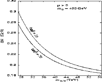
Figure 3.34: Mass difference $\Delta M\equiv m_{\tilde{\chi}_{1}^{\pm}}-m_{\tilde{\chi}_{1}^{0}}$ as a function of the gravitino mass for $\tan\beta=10$ (upper curve) and $\tan\beta=30$ (lower curve), $\mu>0$, and $m_{0}=450~{}{\rm GeV}$.

The lighter chargino thus decays mostly (96-98 %) into the lightest neutralino and a soft $\pi^{\pm}$, possibly with a visibly displaced vertex. Ref. [43] discusses search strategies for the chargino pair production: $e^{+}e^{-}\to\tilde{\chi}_{1}^{+}\tilde{\chi}_{1}^{-}(\gamma)$, where the additional photon will be very useful to suppress the huge two-photon $\pi\pi$ background expected for the $\Delta M$ range shown above, or to tag the chargino pair production when the final-state pions are too soft to be detected. When the decay length is comparable or larger than the detector size, the charginos will appear as heavily ionizing particles as in the case of the slepton LSP in the GMSB models. If the daughter pions are too soft to be detected, one may observe abruptly terminating tracks in the central tracker. Fig. 3.35 summarizes the search methods and corresponding discovery limits shown in the $m_{\tilde{\chi}_{1}^{\pm}}$-$\Delta M$ plane.

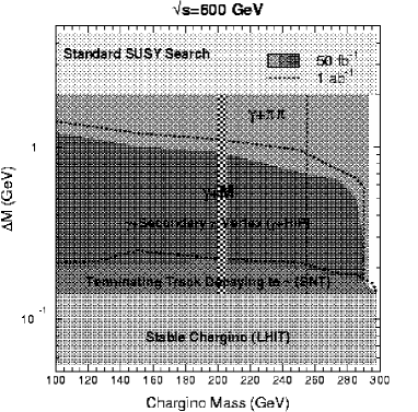
Figure 3.35: Viable search modes in different regions in the $m_{\tilde{\chi}_{1}^{\pm}}$-$\Delta M$ ($\equiv m_{\tilde{\chi}_{1}^{\pm}}-m_{\tilde{\chi}_{1}^{0}}$) plane. Discovery reach is given for $50~{}{\rm fb}^{-1}$ and also for $1~{}{\rm ab}^{-1}$ accumulated at $\sqrt{s}=600~{}{\rm GeV}$. The vertical band and vertical line (the band for $50~{}{\rm fb}^{-1}$ and the line for $1~{}{\rm ab}^{-1}$) is the reach of the $\gamma+\not{\!{M}}$ detection mode, which is relevant only if the $\pi$’s are too soft to detect[43].

The figure tells us that, with all the methods combined, one can cover the parameter space almost to the kinematical limit.

The scalar mass formula also contains a phenomenologically important message that is the near degeneracy of the left- and right-handed sleptons, which means that left- and right-handed sleptons can be produced simultaneously, with relative rates controlled by the beam polarization. Slepton productions are studied[44, 45] in the context of the AMSB models assuming $\sqrt{s}=1~{}{\rm TeV}$.

For instance, let us consider the left-handed selectron pair production:$e^{+}e^{-}\to\tilde{e}_{L}^{+}\tilde{e}_{L}^{-}$ followed by the mixed decays: $\tilde{e}_{L}^{\pm}\to e^{\pm}\tilde{\chi}_{1}^{0}$ and $\tilde{e}_{L}^{\mp}\to\mathop{\nu_{e}}\limits^{\mbox{\scriptsize$(-)$}}\tilde{\chi}_{1}^{\mp}$ with $\tilde{\chi}_{1}^{\mp}$ decaying slowly into $\tilde{\chi}_{1}^{\mp}\to\tilde{\chi}_{1}^{0}+\pi^{\mp}$. This results in a final state: $e^{\pm}\tilde{\chi}_{1}^{0}\mathop{\nu_{e}}\limits^{\mbox{\scriptsize$(-)$}}\tilde{\chi}_{1}^{0}\pi^{\mp}$. The signal is a fast $e^{\pm}+\not{\!{E}}_{T}$ and a soft $\pi^{\mp}$. The soft $\pi$ can give rise to a visibly displaced vertex, if the decay length of the chargino is less than 3cm. If it is longer than 3cm, then one sees a heavily ionizing track of the chargino as discussed above. Fig. 3.36 shows the effective cross sections after cuts to select the signal events as contours in the $m_{3/2}$-$m_{0}$ plane.

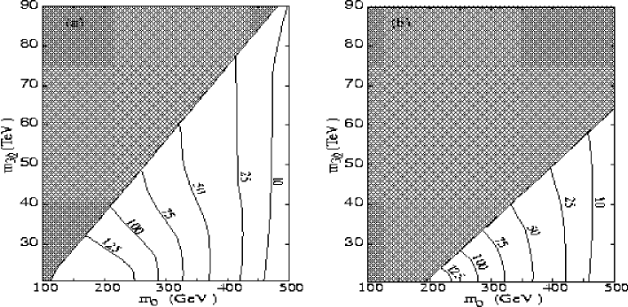
Figure 3.36: Effective cross section contours in the $m_{3/2}$-$m_{0}$ plane expected for the $e^{\pm}\tilde{\chi}_{1}^{0}\mathop{\nu_{e}}\limits^{\mbox{\scriptsize$(-)$}}\tilde{\chi}_{1}^{0}\pi^{\mp}$ signal from $e^{+}e^{-}\to\tilde{e}_{L}^{+}\tilde{e}_{L}^{-}$ at $\sqrt{s}=1~{}{\rm TeV}$: (a) $\tan\beta=3$, and (b) $\tan\beta=30$. The shaded regions are ruled out by various constraints[45].

Note that the effective cross sections include branching fraction as well as the selection efficiency due to the selection cuts. We can see that large regions, allowed by all the current constraints, have large effective cross sections $\sim 10-100$ fb at $\sqrt{s}$ = 1000 GeV.

3.4.5 $\bf\it R$-Parity Violation

Although we have been assuming exact conservation of $R$-parity ($R_{p}$) in the discussions so far, this symmetry is not automatic in the MSSM. Without $R$-parity conservation, the superpotential may contain $R$-parity violating terms:

$$W_{\not{\!{R}}_{p}} = \lambda_{ijk}L_{i}L_{j}e^{c}_{k}+\lambda^{\prime}_{ijk}L_{i}Q_{j}d^{c}_{k}+\lambda^{\prime\prime}_{iji}u^{c}_{i}d^{c}_{j}d^{c}_{k}+\mu_{i}H_{u}L_{i}.$$

The $\lambda$- and $\lambda^{\prime}$-terms violate lepton number ($L$), while the $\lambda^{\prime\prime}$-terms break baryon number ($B$). In order to avoid unacceptably rapid proton decay, the $\not{\!{B}}$ and the $\not{\!{L}}$ terms should not be made finite simultaneously. The $\mu_{i}$ terms are also lepton-number violating, but can be rotated away at tree level.

Here, we assume that these $R$-parity violating couplings are strong enough to make the LSP ($\tilde{\chi}_{1}^{0}$) decay promptly in the detector volume, but other than that they are too weak to participate in the observable phenomena. Let us then consider $e^{+}e^{-}\to\tilde{\chi}_{i}^{+}\tilde{\chi}_{j}^{-}$ and $e^{+}e^{-}\to\tilde{\chi}_{i}^{0}\tilde{\chi}_{j}^{0}$[47]. Once the LEP constraints on $m_{\tilde{\chi}_{1}^{\pm}}$ are imposed, it is found that over a large part of the region of parameter space which allows $\tilde{\chi}_{1}^{+}$ within the reach of a 500 GeV linear collider, $\tilde{\chi}_{3}^{0},\tilde{\chi}_{4}^{0}$, and $\tilde{\chi}_{2}^{+}$ are almost always beyond its reach, at least in the framework of the (c)MSSM. Hence it is sufficient to consider i) $e^{+}e^{-}\to\tilde{\chi}_{1}^{0}\tilde{\chi}_{2}^{0}$, ii)$e^{+}e^{-}\to\tilde{\chi}_{2}^{0}\tilde{\chi}_{2}^{0}$, and iii) $e^{+}e^{-}\to\tilde{\chi}_{1}^{+}\tilde{\chi}_{1}^{-}$. Further, using the approximate degeneracy of $\tilde{\chi}_{1}^{\pm}$ and $\tilde{\chi}_{2}^{0}$, the number of decay chains to be considered are reduced to manageable numbers. The final-state $\tilde{\chi}_{1}^{0}$’s decay via $R$-parity violating terms:

$$LLe^{c}(\lambda) : \tilde{\chi}_{1}^{0}\to l_{1}^{+}l_{2}^{-}+\not{\!{E}}_{T}$$

$$LQd^{c}(\lambda^{\prime}) : \tilde{\chi}_{1}^{0}\to l^{\pm}+\not{\!{E}}_{T}~{}~{}\mbox{or}~{}~{}l^{\pm}+2~{}\mbox{Jets}$$

$$u^{c}d^{c}d^{c}(\lambda^{\prime\prime}) : \tilde{\chi}_{1}^{0}\to 3~{}\mbox{Jets},$$

where $\not{\!{E}}_{T}$’s are due to neutrinos. For the $\not{\!{L}}$ $\lambda$-couplings the final state will consist of $m$ leptons and $\not{\!{E}}_{T}$; for the $\not{\!{L}}$ and $\not{\!{B}}$ $\lambda^{\prime}$-couplings it will consist of $m$ leptons, $n$ jets and $\not{\!{E}}_{T}$, whereas $\not{\!{B}}$ $\lambda^{\prime\prime}$-couplings give rise to a final state with only jets. Potential standard model backgrounds include: $e^{+}e^{-}\to W^{+}W^{-}$, $e^{\pm}\mathop{\nu_{e}}\limits^{\mbox{\scriptsize$(-)$}}W^{\mp}Z$, $ZZ$, $t\bar{t}(g)$, $W^{+}W^{-}Z$, $e^{+}e^{-}Z$, etc.

Table 3.4: Contributions (in fb) of different (light) chargino and neutralino production modes to multi-lepton signals in the case of $\lambda$-couplings for point A of the five points studied[47]: $M_{2}=100~{}{\rm GeV}$, $\mu=-200~{}{\rm GeV}$, $\tan\beta=2$, and $M_{\tilde{e}_{L}}=M_{\tilde{e}_{R}}=150~{}{\rm GeV}$. The last column shows the SM background.

	Signal	$\tilde{\chi}^{0}_{1}\tilde{\chi}^{0}_{1}$	$\tilde{\chi}^{0}_{1}\tilde{\chi}^{0}_{2}$	$\tilde{\chi}^{0}_{2}\tilde{\chi}^{0}_{2}$	$\tilde{\chi}^{+}_{1}\tilde{\chi}^{-}_{1}$	Signal	Bkgd.
						(fb)	(fb)
A	$1\ell+\not{\!{E}}_{T}$	$1.1$	$0.4$	$0.2$	$1.5$	$3.2$	$8272.5$
	$2\ell+\not{\!{E}}_{T}$	$14.9$	$5.2$	$1.8$	$15.3$	$37.2$	$2347.4$
	$3\ell+\not{\!{E}}_{T}$	91.7	25.3	7.2	71.6	195.8	1.5
	$4\ell+\not{\!{E}}_{T}$	212.8	49.6	13.6	152.8	428.8	0.4
	$5\ell+\not{\!{E}}_{T}$	0.0	37.8	19.3	113.5	170.6	-
	$6\ell+\not{\!{E}}_{T}$	0.0	39.6	21.6	26.9	88.0	-
	$7\ell+\not{\!{E}}_{T}$	0.0	0.0	11.9	0.0	11.9	-
	$8\ell+\not{\!{E}}_{T}$	0.0	0.0	8.0	0.0	8.0	-

Table 3.4 shows, for a particular point (point A), results of the Monte Carlo analysis for the case of $\lambda$-couplings. We can see that the requirements of three or more isolated energetic leptons in the final states retains a large fraction of signal events, while suppressing the background to a negligible level. In the case of the $\lambda^{\prime}$-couplings, we can still use the same strategy but with significant loss of signal events due to the smaller expected number of leptons in the final states. Although detailed simulations are yet to be done, the cleanness of the final sample seems to allow mass determinations: we can carry out similar analyses as with the $R$-parity conserving cases by ignoring the decay products of the LSP or, if there is no missing neutrino in the LSP decay, we can directly reconstruct the masses involved in the decay chains.

In the case of $\lambda^{\prime\prime}$-couplings, we can no longer rely on leptons. The final states involve a large number of partons with or without leptons. Some of these partons may merge together in jet definitions, removing the connection between the jet multiplicity and the number of initial partons in the final state. Nevertheless, it is pointed out that kinematic mass reconstructions can be used to study the multi-jet events and identify those coming from $\not{\!{B}}$ couplings. Fig. 3.37 shows the distributions of the invariant mass constructed from the hardest jet and all the other jets in the same hemisphere, and the same for the hardest jet in the opposite hemisphere.

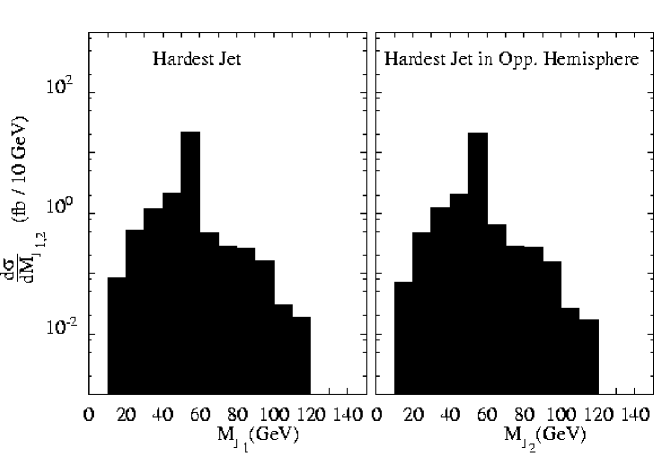
Figure 3.37: Distribution of invariant mass reconstructed from (a) the hardest jet and all jets in the same hemisphere, and (b) the hardest jet in the opposite hemisphere and all remaining hadronic jets, when all contributions are summed over (signal only), for a chosen point in the parameter space[47].

The distribution shows clear peaking at $m_{\tilde{\chi}_{1}^{0}}$ as well as a sharp cutoff at $m_{\tilde{\chi}_{1}^{\pm}}\approx m_{\tilde{\chi}_{2}^{0}}$. Thus kinematic distributions can be used quite effectively even for the case of the multi-jet events.

3.5 Requirements to Machine and Detector

Most of the studies presented above assumed an integrated luminosity ranging from $20$ to $100~{}{\rm fb}^{-1}$, where measurement accuracy is largely limited by statistical errors. Recent progress of machine technology, however, allows us to think about much higher luminosity than one could hope at the time of the green book writing[2]. In this context, we will examine here how the detector resolution or the machine energy uncertainty might affect the SUSY study scenarios we discussed so far.

Major roles of the detector components are listed below:

• Heavy flavor ID. Particularly important, if one wants to fully reconstruct chargino pair production in the 4-jet mode in combination with particle ID information. It is also important for detecting visibly displaced decay vertices of the LSP as expected in GMSB models.

• Good end-point energy resolution for leptons. The central tracker will also be essential to achieving good energy flow measurement for end-point energy resolution for jets. Energy loss measurement for GMSB staus. Some care must be taken for triggering such heavy and therefore slowly moving stable particles.

• Good energy flow measurement for end-point energy resolution for jets. Vertex pointing resolution for the GMSB neutralino. Low angle coverage to push $\theta_{min}$ as much as possible down to the beam line.

• $K/\pi$ separation might be important to decide the charge of a $c(\bar{c})$-jet from, for instance, $W$ bosons produced in the chargino decays: full reconstruction of the chargino pair production then becomes possible.

Taking into account that the SUSY studies we have discussed above are largely based on the precision measurements of the masses and polarization-dependent cross sections (mixings) of the sparticles, we focus, in what follows, our attention on effects of the detector and machine performance on these measurements.

3.5.1 End-Point Measurements

Let us begin with the end-point measurement, since it is not only one of the most important experimental techniques but also a typical place where detector and machine energy resolutions might play some important role, once the integrated luminosity well exceeds $100~{}{\rm fb}^{-1}$.

First of all, it should be noted that initial-state radiation (ISR) and beamstrahlung do not change the end-point locations, since the reduction of the effective beam energy, if sizable, makes the higher end-point ($E_{+}$) lower and the lower end-point ($E_{-}$) higher. Fig. 3.38 clearly demonstrates this fact.

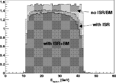
Figure 3.38: Muon energy distributions for $e^{+}e^{-}\to\tilde{\mu}_{R}^{+}\tilde{\mu}_{R}^{-}$ followed by $\tilde{\mu}_{R}^{\pm}\to\mu^{\pm}\tilde{\chi}_{1}^{0}$ (dotted) with neither ISR nor beam effects (BM), (dot-dashed) with ISR only, and (solid) with both ISR and beam effects. The Monte Carlo data correspond to Fig. 3.4 and were generated at $\sqrt{s}=350~{}{\rm GeV}$ with $m_{0}=70~{}{\rm GeV}$, $M_{2}=250~{}{\rm GeV}$, $\mu=400~{}{\rm GeV}$, and $\tan\beta=2$.

Consider a two-body decay of a particle with mass $M$ to a lepton (muon in our case) and a massive daughter with mass $m$. Ignoring the lepton mass, $M$ and $m$ can be expressed in terms of the end points, $E_{+}$ and $E_{-}$ as

$$\left\{\begin{array}[]{lll}M&=&2E\frac{\sqrt{E_{+}E_{-}}}{E_{+}+E_{-}}\cr&&\cr\frac{m}{M}&=&\sqrt{\frac{E-(E_{+}+E_{-})}{E}},\end{array}\right.$$ (3.27)

where $E$ is the beam energy. This leads, for instance, to the following formula for the relative error on the parent mass:

$$\sigma_{M} = \left(\frac{M}{2}\right)\left(\frac{E_{+}-E_{-}}{E_{+}+E_{-}}\right)\sqrt{\left(\frac{\sigma_{E_{+}}}{E_{+}}\right)^{2}+\left(\frac{\sigma_{E_{-}}}{E_{-}}\right)^{2}}.$$

Since the lepton energy will be measured by the central tracker that has energy (momentum) resolution that is proportional to the energy: $\sigma_{E}/E=aE$, The above equation becomes:

$$\sigma_{M} = \left(\frac{M}{2}\right)\left(\frac{E_{+}-E_{-}}{E_{+}+E_{-}}\right)a\sqrt{E_{+}^{2}+E_{-}^{2}}.$$

Using this formula, we can translate the current performance goal of the central tracker, $a\simeq 5\times 10^{-5}~{}{\rm GeV}^{-1}$, to the $\sigma_{M}$ of about $0.1~{}{\rm GeV}$ for the example shown in Fig. 3.4 or in Fig. 3.38. This value should be compared with $\sigma_{M}\simeq 0.7~{}{\rm GeV}$ expected for $20~{}{\rm fb}^{-1}$ (see Fig. 3.4). Assuming that this statistical error scales as $1/\sqrt{N}$, we expect $\sigma_{M}\simeq 0.1~{}{\rm GeV}$ for an integrated luminosity of $1~{}{\rm ab}^{-1}$, which is comparable with the detector resolution. This means that the tracker resolution is good enough for the measurement, provided that we understand the detector performance well.

For the chargino mass determination, we need to retain the $W$ mass in the end-point formula:

$$M = \sqrt{2}E\frac{\sqrt{E_{+}E_{-}+m_{W}^{2}+\sqrt{(E_{+}^{2}-m_{W}^{2})(E_{-}^{2}-m_{W}^{2})}}}{E_{+}+E_{-}},$$

from which we obtain

$$\sigma_{M}^{2} = \left(\frac{\partial M}{\partial E_{+}}\right)^{2}\sigma_{E_{+}}^{2}+\left(\frac{\partial M}{\partial E_{-}}\right)^{2}\sigma_{E_{-}}^{2}.$$

with

$$\left(\frac{\partial M}{\partial E_{\pm}}\right)^{2} = \left(\frac{M}{E_{+}+E_{-}}\right)\left[\left(\frac{E}{M}\right)^{2}\frac{E_{\mp}+E_{p}m\sqrt{\frac{E_{\mp}^{2}-m_{W}^{2}}{E_{\pm}^{2}-m_{W}^{2}}}}{E_{+}+E_{-}}-1\right].$$

Notice that, since we need to rely on the energy flow measurement for jets, we need to use

$$\sigma_{E_{\pm}}/E_{\pm} = b/\sqrt{E_{\pm}}.$$

The detector resolution is already important for the integrated luminosity of $50~{}{\rm fb}^{-1}$ assumed in Fig. 3.10, even if we assume currently conceivable best energy flow resolution: $b\simeq 0.1~{}{\rm GeV}^{-1/2}$ corresponding to $\sigma_{M}\simeq 8~{}{\rm GeV}$. This means that we need to understand the resolution function to the accuracy that stands up to the expected statistical error.

On the other hand, the mass determination by means of threshold scan will be rather insensitive to the detector resolution and potentially more accurate in particular for spin 1/2 particles with rapidly rising cross sections[48]. This technique might, however, be affected by the natural beam energy spread and beamstrahlung. Fig. 3.39 shows the effects of ISR and the beam effects on the threshold shape of the $e^{+}e^{-}\to\tilde{\mu}_{R}^{+}\tilde{\mu}_{R}^{-}$ process.

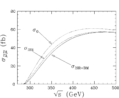
Figure 3.39: Production cross sections for $e^{+}e^{-}\to\tilde{\mu}_{R}^{+}\tilde{\mu}_{R}^{-}$ (dotted) with neither ISR nor beam effects (BM), (dot-dashed) with ISR only, and (solid) with both ISR and beam effects. The SUSY parameters are the same as with Fig 3.38: with $m_{0}=70~{}{\rm GeV}$, $M_{2}=250~{}{\rm GeV}$, $\mu=400~{}{\rm GeV}$, and $\tan\beta=2$.

If we are to carry out threshold scan we need to understand the energy distribution of the collider very well. It should also be noted that the branching fraction to the final states to be used for a threshold scan is not a priori known, which forces us to make the overall normalization a free parameter in the fit. Moreover, the cross sections in particular for the second and the third-generation sneutrinos are not necessarily large enough to carry out their threshold scan with a practicable luminosity[49].

3.5.2 Beam Polarization

It has been stressed many times that the beam polarization plays a crucial role in sorting out the sparticle mixings. For instance, let us recall the mixing angle determination for the stau. The production cross section for the $e^{+}e^{-}\to\tilde{\tau}_{1}^{+}\tilde{\tau}_{1}^{-}$ process depends on the electron beam polarization, as well as on the stau mixing angle $\theta_{\tau}$ as shown in Fig. 3.40.

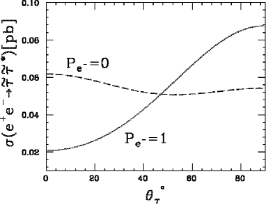
Figure 3.40: The mixing angle ($\theta_{\tau}$) dependence of the production cross section of $\tilde{\tau}_{1}\tilde{\tau}_{1}$ for $m_{\tilde{\tau}}=150$ GeV and $\sqrt{s}=500$ GeV. The cross section is heavily dependent on $\theta_{\tau}$ for the right-handed electron beam ($P_{e}=1$).

This suggests that, even if we perfectly understand the effective center of mass energy distribution (beam effects) of the machine, there can still be some uncertainty due to the error in the beam polarization measurements. The expected error on the mixing angle was estimated to be $\Delta\sin\theta_{\tau}/\sin\theta_{\tau}\simeq 0.065$ (see Section 3.3.6) for an integrated luminosity of $100~{}{\rm fb}^{-1}$. This implies that for $1~{}{\rm ab}^{-1}$, the statistical error reaches $2~{}\%$ level. The error on the beam polarization must thus be controlled down to $1~{}\%$ level or less. It should also be pointed out that the higher the beam polarization, the easier the mixing angle determinations through polarization-dependent cross section measurements. In this respect, the positron beam polarization is useful. The power of the positron beam polarization is, however, further enhanced for the SUSY processes with $t$-channel neutralino exchanges, since the neutralinos, being of Majorana type, do not respect the automatic helicity selection rule between the electron and the positron beams. As we have seen in the $CP$ violation studies, transverse beam polarization is also a useful option to consider.

3.5.3 Forward/Backward Detector to Veto Low Angle $\bf e^{+}e^{-}$

For detecting missing $P_{T}$ signals of sparticle productions, it is essential to be able to veto low angle $e^{+}/e^{-}$’s to suppress two-photon backgrounds. Fig. 3.42 shows the $P_{T}$ distributions of the signal ($e^{+}e^{-}\to\tilde{\tau}_{1}^{+}\tilde{\tau}_{1}^{-}$) and the background ($e^{+}e^{-}\rightarrow e^{+}e^{-}\tau^{+}\tau^{-}$), for $\theta_{acop}>30^{\circ}$ and $|\cos\theta_{jet}|<0.8$. When the minimal veto angle ($\theta^{veto}_{e}$) for forward and backward electrons and positrons is 150 mrad, the background rate is intolerable high up to $P_{T}<35$ GeV.

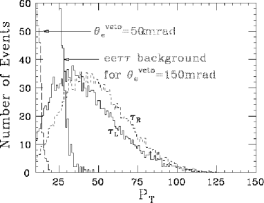
Figure 3.41: $P_{T}$ distributions for the signal and the background $e^{+}e^{-}\tau^{+}\tau^{-}$ events at $\sqrt{s}=500$ GeV after the cuts: $|\cos\theta_{jet}|<0.8$ and $\theta_{acop}>30^{\circ}$, for different minimum veto angles. $10^{4}$ signal events were generated with $m_{\tilde{\tau}}=150$ GeV and $m_{\tilde{\chi}^{0}_{1}}=100$ GeV, corresponding to $\int Ldt=100$ $fb^{-1}$.

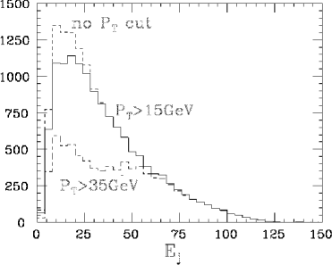
Figure 3.42: $P_{T}$ cut dependence of the energy distribution of the final-state hadrons from the stau decays. The $P_{T}$ cut at 35 GeV significantly distorts the energy distribution near its peak.

If $\theta^{veto}_{e}=$ 150 mrad we thus need to require $P_{T}>35$ GeV, which distorts the energy distribution significantly and reduces the reliability of the mass determination in this method (see Fig. 3.42). On the other hand, for $\theta^{veto}_{e}$ = 50 mrad, the cut on $P_{T}$ can be lowered to about 15 GeV, which makes the resultant energy distribution much less affected. It is thus essential to push the minimum veto angle down to at least $50$ mrad.

3.6 Tests of SUSY Breaking Mechanisms

We have seen above that the precision measurements of the masses and the mixings in the sfermion and the chargino/neutralino sector will certainly allow us to quantitatively test various supersymmetry relations, thereby firmly establishing the existence of supersymmetry as a dynamical symmetry of particle interactions. More importantly, the precision we expect for these measurements at the JLC is so high that we will be able to infer the SUSY breaking scale and the values of the SUSY breaking parameters at this high scale. Since these SUSY breaking parameters are presumably determined by the physics at the high scale, this will open up a first realistic way to systematically study the physics at this high scale experimentally.

Some examples of such studies are already mentioned above, including tests of universality among scalar masses and gaugino mass unification expected in the SUGRA models. These tests can be carried out step by step in the course of the SUSY discovery and study scenarios. We can hope that, eventually, we will be able to determine all the masses and the mixings of the sparticle spectrum, thereby fixing all of the Lagrangian parameters such as $M_{1},M_{2},\mu,\tan\beta$ at the electroweak (EW) scale. In this section, we review what and to what extent we can learn then from these precision measurements of the masses and the mixings.

One can use these accurately determined Lagrangian parameters at the EW scale to fit their values at the high scale. It has been shown [48] in this approach, that the projected accurate measurements of the various sparticle masses through an energy scan for each sparticle’s threshold, using ten energy points with $10$ ${\rm fb}^{-1}$ each, allows one to determine $M_{1},M_{2},m_{0},\mu$, and $\tan\beta$ at the high scale to an accuracy better than $1\%$. The accuracy is much worse, however, for higher values of $\tan\beta$. The expected accuracy for the trilinear term is rather poor as shown in Tables 3.6 and 3.6 taken from Ref. [48], which is due to the fact that most of the physical observables are rather insensitive to the parameters $A_{k}$.

Table 3.5: Reconstruction of SUGRA parameters assuming universal masses.

	True value	Error
$m_{0}$	100	0.09
$m_{1/2}$	200	0.10
$A_{0}$	0	6.3
tan$\beta$	3	0.02

Table 3.6: Reconstruction of SUGRA parameters with nonuniversal gaugino masses.

	True value	Error
$m_{0}$	100	0.09
$M_{1}$	200	0.20
$M_{2}$	200	0.20
$A_{0}$	0	10.3
tan$\beta$	3	0.04

In this approach model selection will be made on the basis of goodness of the fit.

There is, however, a totally different approach to test the SUSY breaking mechanisms, the bottom up approach[50], where one starts with these Lagrangian parameters extracted at the EW scale and extrapolates them to the high scale using the renormalization group evolution (RGE). As explained in Section 3.2, different SUSY breaking mechanisms predict different relations among these parameters at the high scale. In the bottom up approach, one can test these relations directly by reconstructing them from their low energy values using the RGE. In Ref.[50], experimental values of the various sparticle masses are generated in a given scenario (mSUGRA, GMSB etc.), by starting from the universal parameters at the high scale appropriate for the model under consideration and evolving them down to the EW scale. These masses are then endowed with experimental errors expected to be reached eventually in the combined analyses of data from LHC and a TeV scale linear collider with an integrated luminosity of $1{\rm ab}^{-1}$. These measured values are then evolved back to the high scale. The left two plots in Fig. 3.43

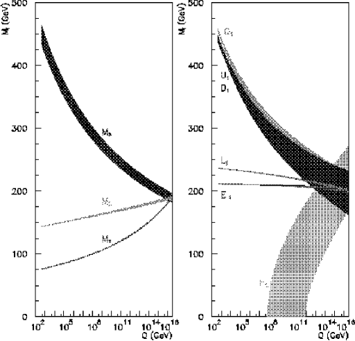
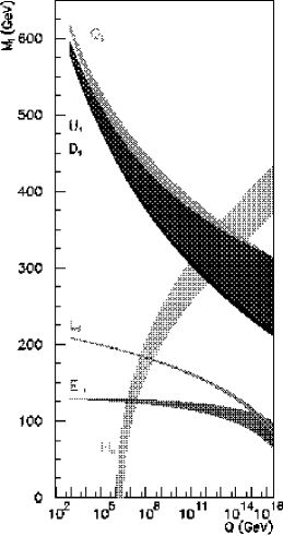
Figure 3.43: Bottom up approach of the determination of the sparticle mass parameters for mSUGRA and GMSB[50]. Values of the model parameters as given there.

show results of such an exercise for the gaugino and sfermion masses, respectively, for the mSUGRA case, while the one on the right for sfermion masses in GMSB. The width of the bands indicates $95\%$ C.L. limits.

We can see that with the projected accuracies of measurements, the unification of the gaugino masses will be indeed demonstrated very clearly in the mSUGRA case. The extrapolation errors for the evolution of the slepton masses are also small, since only the EW gauge couplings contribute to it, and allows one to test the unification of the slepton masses at the high scale. This is in contrast to the squark and higgs masses, for which the extrapolation errors are rather large. In the case of the Higgs mass parameters this insensitivity to the common scalar mass $m_{0}$ is due to an accidental cancellation between different contributions in the loop corrections to these masses which in turn control the RG evolution. In the case of the squarks the extrapolation errors are caused by the stronger dependence of the radiative corrections on the common gaugino mass, due to the strong interactions of the squarks. As a result of these the small error at the EW scale expands rapidly, when extrapolated to the unification scale. It should also be noted that the trilinear $A$ coupling for the top shows a pseudo fixed point behavior, which also makes the EW scale value insensitive to $m_{0}$. If the universal gaugino mass $m_{1/2}$ is larger than the $m_{0}$ then this pseudo fixed point behavior increases the errors in the determination of the third generation squark mass at the EW scale. This picture shows us clearly the extent to which the unification at high scale can be tested. If we compare this with the results of Tables 3.6 and 3.6, we see that with the bottom up approach we have a much clearer representation of the situation. It should be stressed that the $95\%$ C.L. bands on the squark and the higgs mass parameters become much wider if one only assumes the accuracies expected to be reached at the LHC[51]. The linear collider’s precision measurements are indispensable to get a clearer picture of the SUSY breaking mechanism at the high scale.

The right-most plot in Fig. 3.43 shows the results of a similar exercise but for the GMSB model, where with the assumed values of the model parameters, one would need to have a $1.5$ TeV linear collider to access the full sparticle spectrum. In this case the doublet slepton mass and the Higgs mass parameter are expected to unify at the messenger scale, which the data show quite clearly. It is remarkable that the extrapolation of the reconstructed slepton and squark masses to the high scale is stable enough to reveal the entirely different unification patterns expected in this case as opposed to the mSUGRA case. The bottom up approach of testing the structure of the SUSY breaking sector definitely requires the high accuracy that can be achieved only with the linear collider[51].

All of these discussions assume that most of the sparticle spectrum are accessible jointly by the LHC and a TeV scale linear collider. If we are unlucky and the squarks are super-heavy, then perhaps the only clue to their existence can be obtained through the analogue of precision measurements of the oblique correction to the SM parameters at the $Z$ pole. These super-oblique corrections [53] modify the tree-level supersymmetry relations between various couplings as already mentioned in Section 3.3.2. These modifications arise if there is a large mass splitting between the sleptons and the squarks. The expected radiative corrections imply

$${{\delta g_{Y}}\over g_{Y}} \simeq {{11g_{Y}^{2}}\over{48\pi^{2}}}ln\left({m_{\tilde{q}}}\over{m_{\tilde{l}}}\right),$$ (3.28)

which amounts to about $0.7\%$, if the mass splitting is a factor of 10. We have shown in the previous sections that it might well be possible to make a measurement with such accuracy at the JLC.

Chapter 4 Top Quark Physics

4.1 Introduction

Among all the fermions included in the Standard Model (SM), the top quark plays a very unique role. The mass of the top quark is by far the largest and approximates the electroweak (EW) symmetry breaking scale. The recent reported value from the CDF and D0 collaborations reads

$$m_{t}=174.3\pm 3.2(stat)\pm 4.0(syst)~{}\mbox{GeV}~{}~{}~{}~{}~{}\mbox{(CDF+D0 combined\cite[cite]{[\@@bibref{}{moriond2000}{}{}]})}.$$ (4.1)

In fact the top quark is the heaviest of all the elementary particles discovered up to now. It means that in the SM Lagrangian the top quark mass term breaks the $SU(2)_{L}\times U(1)_{Y}$ symmetry maximally. This fact suggests that the top quark couples strongly to the physics that breaks the EW symmetry. It is therefore important to investigate properties of the top quark in detail, for the purpose of probing the symmetry breaking physics as well as to gain deeper understanding of the origin of the flavor structure. The standard procedures for investigating top quark properties are: measurements of fundamental quantities such as its mass and decay width; detailed examinations of various interactions of top quark to see if there are signs of new physics.

Studies of various properties of the top quark have been started at Tevatron. For example, the polarization of $W$ bosons from the decay of top quarks has been measured. More detailed properties will be investigated further in future experiments at Tevatron Run II, at LHC and at JLC. In particular, experiments at JLC will be able to uncover detailed properties through precision measurements of various top quark interactions. For example, another fundamental parameter of the top quark, its decay width $\Gamma_{t}$, can be measured accurately. Within the SM the top quark decays almost 100% to the $b$ quark and $W$. The width can be predicted as a function of $m_{t}$, $\alpha_{s}$, $M_{W}$, etc. Already a fairly precise theoretical prediction at the level of a few percent accuracy is available [2]. Here, we only note that $\Gamma_{t}\simeq 1.5$ GeV for the above top quark mass range. This value deviates with simple extensions of the SM: e.g. $\Gamma_{t}\propto|V_{tb}|^{2}$ can be smaller if there is a fourth generation, whereas it will be greater if there are additional decay modes such as $t\to bH^{+}$ or $t\to\tilde{t}\tilde{\chi}$. Thus, it is important to measure $\Gamma_{t}$ precisely. An important property of the top quark, besides its heaviness, is that it decays so quickly that no top-hadrons will be formed. Therefore all the spin information of the top quark will be transferred to its decay daughters in its decay processes [3], and the energy-angular distributions of the decay products are calculable as purely partonic processes. In fact we may take full advantage of the spin information in studying the top quark properties through its decay processes [4].

In this chapter we review the studies of top quark physics at JLC. We will first focus on the prospects in the $t\bar{t}$ threshold region in three steps: In Subsection 4.2.1 we clarify the physics motivation and goals; In Subsection 4.2.2 we discuss the precision measurements of the top quark mass; In Subsection 4.2.3 we discuss the relevant observables; Subsection 4.2.4 is devoted to the sensitivity studies on various top quark couplings. In the rest, we will discuss the physics in the open top region. In Section 4.3 we discuss a measurement of $m_{t}$ from the dilepton events. In Section 4.4 measurement of the top-Yukawa coupling is studied. In Section 4.5 anomalous couplings of the top quark with the Higgs boson are studied. In Section 4.6 anomaly in the Standard-Model top quark interactions is studied through the decay processes of the top quark. In Section 4.7 we study how to probe $CP$ violation in the open top region, using both $e^{+}e^{-}\to t\bar{t}$ and $\gamma\gamma\to t\bar{t}$ processes. On the other hand, Section 4.8 examines the possibility to observe $R$-parity violating SUSY interactions using the top quark. We summarize our studies in Section 4.9.

4.2 Top Quark Threshold Region

An experiment in the top quark threshold region ($\sqrt{s}\approx 2m_{t}$) is considered as a serious candidate for the first stage operation of JLC. In this section we review the subjects that can be covered in experiments in the $t\bar{t}$ threshold. We will be able to extract rich physics and test properties of the top quark in detail.

4.2.1 Physics Motivations and Goals

The major three goals that should be achieved in the experiment in the $t\bar{t}$ threshold region will be as follows:

• A precision measurement of the top quark mass.

• To elucidate dynamics involved in formations and decays of (remnants of) the toponium resonances.

• Tests of the various top quark interactions: search for anomalies in the $t\bar{t}\gamma$, $t\bar{t}Z$, $tbW$, $ttg$ and $ttH$ couplings and possibly for other non-SM interactions.

Here, we briefly explain the physics motivation for each of these goals.

1) Top Mass Determination

The top quark mass $m_{t}$ is one of the fundamental parameters of the SM. It is conceivable that, in the future, to know its precise value will be crucial to achieve a high predictive power in precision physics. In fact some important observables depend on $m_{t}$ sensitively through radiative corrections, when $m_{t}$ acts as a non-decoupling parameter. Then it is required that $m_{t}$ should be known more precisely than other parameters of the theory. For example, suppose that the Higgs boson is discovered in the future, and suppose that we want to test predictions of its mass by the Minimal Supersymmetric Model within 50 MeV accuracy. Then we need to know the top quark mass with a similar accuracy due to the large dependence of the radiative correction on the top quark mass: $\delta m_{H}^{2}\sim G_{F}m_{t}^{4}\ln(m_{\tilde{t}_{1}}m_{\tilde{t}_{2}}/m_{t}^{2})$.

2) Testing Dynamics of $t\bar{t}$ Resonances

On the one hand, we will be able to observe intriguing phenomena of the (remnants of) $t\bar{t}$ resonances which are quite different from the phenomenology of charmonium and bottomonium. This is because: (1) The top quarks decay via the EW interaction very quickly, and the decay daughters carry the information on the dynamics of the top quarks inside the resonances. (2) The interplays of the QCD and EW interactions induce unique phenomena. On the other hand, due to the large mass and the large decay width of the top quark, high precision theoretical predictions based on the first principles are available. Therefore we will be able to make detailed tests of the dynamics of the boundstate formation and decays. This aspect is important since predictability of the theory on the quarkonium physics has improved dramatically recently. For example, so far the quarkonium wave functions calculated in perturbative QCD have never been tested experimentally, and this will be possible for the $t\bar{t}$ resonances.

3) Examinations of Various Top Quark Interactions

Studies of various top quark interactions will be pursued both in the open top region, where we can explore more deeply into the structures of many of the interactions, and in the $t\bar{t}$ threshold region. There are specific advantages in each case. The advantages in the $t\bar{t}$ threshold region are as follows. First, to study the decay properties of the top quark, the threshold region will be optimal. This is because: the top quark can be polarized maximally by polarizing the electron beam; we are guaranteed to be (almost) in the rest frame of the top quark without need to reconstruct its momentum; we do not gain resolving power by raising the c.m. energy. In particular, the top quark decay width can be measured most precisely in the threshold region. Secondly, we can test not only the EW interactions of the top quark but also the QCD interactions. Since the threshold cross section includes an infinite number of $ttg$ couplings at leading order, it has a high sensitivity also to the anomalous $ttg$ couplings.

4.2.2 Top Quark Mass

How to Determine the Mass

The top quark mass will be determined to high accuracy from the shape of the $t\bar{t}$ total production cross section in the threshold region [5]. If the top quark were stable, the cross section would show distinct resonance peaks in this region. Due to the large decay width of the top quark, $\Gamma_{t}\simeq 1.5$ GeV, however, these peaks will be smeared out. The resonances merge with one another, leading to a broad enhancement of the cross section over the threshold region; see Fig. 4.1.

Figure 4.1: The total cross section vs. energy, $E=\sqrt{s}-2m_{t}$. The solid curve is calculated from the Green function. The dashed curve shows the tree-level total cross section for a stable top quark.

Still, the location of the sharp rise of the cross section is determined mainly from the mass of the lowest-lying ($1S$) $t\bar{t}$ resonance. Since the mass of the resonance can be calculated as a function of the top quark mass and $\alpha_{s}$ from perturbative QCD, we will be able to extract the top quark mass from the measurement of the $1S$ peak position of the cross section.

In the beginning of the studies of the threshold cross section, people planned to extract the pole-mass of the top quark from the cross section. This is because the position of the “threshold” is determined as twice the top quark pole-mass, and it was considered most natural to relate this mass parameter directly to the threshold cross section or the resonance spectrum. On the other hand, existence of the pole-mass of a quark contradicts the confinement picture of QCD and this mass is most likely to be ill-defined beyond perturbation theory; even within perturbative QCD we face a problem in any attempt to define this quantity to ${\cal O}(\Lambda_{QCD})={\cal O}$(300 MeV) or better. Recently there has been significant progress in our theoretical understanding of heavy quarkonia such as $\Upsilon$’s and (remnant of) toponium resonances. Developments in technologies of higher-order calculations and the subsequent discovery of renormalon cancellation enabled extractions of the top quark mass with high accuracy in future experiments. It became clear that we have to relate the threshold cross section to a short-distance mass, such as the $\overline{\rm MS}$ mass, in order to extract a precise and physically meaningful mass parameter.

The upshot of the theoretical studies up to now is as follows. The series expansion of the mass of (remnant of) the $1S$ $t\bar{t}$ resonance in $\alpha_{s}$ becomes much more convergent when we express the series in terms of the $\overline{\rm MS}$ mass of the top quark instead of the pole-mass. At the present situation, theoretical uncertainty of the $\overline{\rm MS}$ mass $\overline{m}_{t}\equiv m_{t}^{\overline{\rm MS}}(m_{t}^{\overline{\rm MS}})$ is about 150 MeV when we determine it from the threshold scan. Also, concerning future prospects, there seems to be a good chance to reduce the theoretical uncertainty to about 50 MeV by the time of the JLC operation.

Simulation Studies on Expected Precision

There have been a number of simulation studies which incorporate realistic experimental conditions expected at JLC. Here, we quote the result of the study [5] on the determination of the peak position of the $t\bar{t}$ production cross section, from which the $\overline{\rm MS}$ mass of the top quark $\overline{m}_{t}$ can be extracted. The effects of the beam energy spread and the beamstrahlung as well as those of the initial state radiation are important when studying the threshold cross section. In particular the beam energy spread smears out the $1S$ peak of the cross section. In order to determine the peak position of the original cross section, we convolute the original cross section with the radiator function and with the beam energy spectrum, and then we fit it to the measured cross section. Selection of top quark events can be performed with high efficiency and good background suppression. (More details will be explained in Subsection 4.2.4.) Taking these into account, a simulation study of the energy scan of the cross section was performed. Using 11 energy points with 1 fb^-1 each, we can determine the peak position with a statistical error $\approx 200$ MeV, which translates to a statistical error on the top quark $\overline{\rm MS}$ mass of $\Delta\overline{m}_{t}\approx 100$ MeV.

4.2.3 Observables

In this subsection we discuss the observables which contain interesting information close to the top quark threshold. Here, we restrict ourselves to qualitative arguments. More quantitative analyses will be given in the next subsection.

A) Production Process of Top Quarks

Total Cross Section

The first observable we measure in the $t\bar{t}$ threshold region will be the total cross section. The total cross section can be written as [6, 7]

$$\sigma_{\rm tot}(e^{+}e^{-}\to t\bar{t})\propto-{\rm Im}\sum_{n}\frac{|\psi_{n}({\bf{0}})|^{2}}{E-E_{n}+i\Gamma_{t}}.$$ (4.2)

One sees that the energy dependence of the total cross section is determined by the resonance spectra. Due to the large width $\Gamma_{t}$ of the top quark, however, distinct resonance peaks are smeared out. The resonances merge with one another, leading to a broad enhancement of the cross section over the threshold region as seen in Fig. 4.1. (We will show explicitly the resonance spectra below.) In the same figure, the tree level cross section is also shown as a dashed curve. Despite the disappearance of each resonance peak, one sees that the cross section is indeed largely enhanced by the QCD interaction, and that inclusion of the QCD binding effect is mandatory for a proper account of the cross section in the threshold region.

Top Momentum Distribution

Next we consider the top-quark momentum ($|{\bf{p}}_{t}|$) distribution near $t\bar{t}$ threshold [8, 9]. It has been shown that experimentally it will be possible to reconstruct the top-quark momentum ${\bf{p}}_{t}$ from its decay products with reasonable resolution and detection efficiency. Fig. 4.2(a) shows a comparison of reconstructed top momenta (solid circles) with that of generated ones (histogram), where the events are generated by a Monte Carlo generator and are reconstructed after going through detector simulators and selection cuts; see Subsection 4.2.4 for details. The figure demonstrates that the agreement is fairly good.

Theoretically, the top-quark momentum distribution is given by

$$\frac{d\sigma}{d|{\bf{p}}_{t}|} \propto \biggl{|}\sum_{n}\frac{\phi_{n}({\bf{p}}_{t})\psi_{n}^{*}({\bf{0}})}{E-E_{n}+i\Gamma_{t}}\biggl{|}^{2}+\mbox{(sub-leading)}.$$ (4.3)

The $|{\bf{p}}_{t}|$-distribution is thus governed by the momentum-space wave functions of the resonances. By measuring the momentum distribution, essentially we measure (a superposition of) the wave functions of the toponium resonances. Shown in Fig. 4.2(b) are the top momentum distributions for various energies.

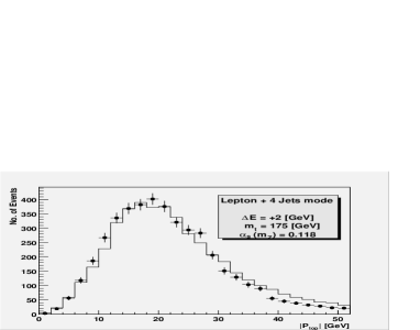
Figure 4.2: (a) Reconstructed momentum distribution (solid circles) for the lepton-plus-4-jet mode, compared with the generated distribution (histogram). The Monte Carlo events were generated with $\alpha_{s}(M_{Z})=0.12$ and $m_{t}=150$ GeV [5]. (b) Top-quark momentum distributions $d\sigma/d|{\bf{p}}_{t}|$ for various c.m. energies measured from the lowest lying resonance, $\Delta E=\sqrt{s}-M_{1S}$, taking $\alpha_{s}(M_{Z})=0.118$ and $m_{t}=175$ GeV.

One may also vary the magnitude of $\alpha_{s}$ and confirm that the distribution is indeed sensitive to the resonance wave functions [8, 9]. Hence, the momentum distribution provides information independent of that from the total cross section.

Forward-Backward Asymmetry

Another observable that can be measured experimentally is the forward-backward asymmetry of the top quark [10]. Generally in a fermion pair production process, a forward-backward asymmetric distribution originates from an interference of the vector and axial-vector $f\bar{f}$ production vertices at tree level of electroweak interaction. One can show from the spin-parity argument that in the threshold region the $t\bar{t}$ vector vertex creates S-wave resonance states, while the $t\bar{t}Z$ axial-vector vertex creates P-wave states. Therefore, by observing the forward-backward asymmetry of the top quark, we observe an interference of the S-wave and P-wave states.

In general, S-wave resonance states and P-wave resonance states have different energy spectra. So if the c.m. energy is fixed at some resonance in either one of the spectra, there would be no contribution from the other. However, the widths of resonances are large for the toponium in comparison to their level splittings, which permit sizable interferences of the $S$-wave and $P$-wave states. Fig. 4.3 shows the pole position $E_{n}\!-\!i\Gamma_{t}$ of these states on the complex energy plane.

Figure 4.3: The positions of poles of the S-wave and P-wave states on the complex energy plane, together with the forward-backward asymmetry as a function of the energy, taking $\alpha_{s}(M_{Z})=0.118$ and $m_{t}=175$ GeV. The right-axis is for the forward-backward asymmetry.

One sees that the widths of the resonances are comparable to the mass difference between the lowest lying S-wave and P-wave states, and exceeds by far the level spacings between higher S-wave and P-wave states. This gives rise to a forward-backward asymmetry even below threshold, and provides information on the resonance level structure which is concealed in the total cross section. Shown on the same figure is the forward-backward asymmetry as a function of the energy. It is seen that the asymmetry takes its minimum value at around the lowest lying S-wave state, where the interference is smallest, and increases up to $\sim 10$% with energy as the resonance spectra appear closer to each other. One may also confirm that essentially the forward-backward asymmetry measures the degree of overlap of the S-wave and P-wave states by varying the coupling constant $\alpha_{s}$ or the top quark decay width $\Gamma_{t}$.

B) Decay of Top Quarks and Final-State Interactions

We turn to decay processes of the top quark near threshold. The top quarks produced via $e^{+}e^{-}\to t\bar{t}$ in the threshold region will be highly polarized [3]. Therefore, the threshold region can be an ideal place for studying properties of the top quark through decay processes, using the highly polarized top quark sample.

Decay of Free Polarized Top Quarks

Detailed studies of the decay of free polarized top quarks have already been available including the full ${\cal O}(\alpha_{s})$ corrections [12, 13, 14]. The best example is the energy-angular distribution of charged leptons $l^{+}$ in the semi-leptonic decay of the top quark. At leading order, the $l^{+}$ distribution has a form where the energy and angular dependences are factorized [15, 16]:

$$\frac{d\Gamma_{t\to bl^{+}\nu}({\bf{S}})}{dE_{l}d\Omega_{l}}=h(E_{l})\,(1+|{\bf{S}}|\cos\theta_{l})~{}~{}+~{}~{}[\,{\cal O}(\alpha_{s})~{}\mbox{correction}\,].$$ (4.4)

Here $E_{l}$, $\Omega_{l}$, and $\theta_{l}$ denote, respectively, the $l^{+}$ energy, the solid angle of $l^{+}$, and the angle between the $l^{+}$ direction and the top polarization vector ${\bf{S}}$, all of which are defined in the top-quark rest frame. Hence, we may measure the top-quark polarization with maximal sensitivity using the $l^{+}$ angular distribution.

Effects of Final-State Interactions

Close to threshold, the above precise analyses of the free top-quark decays do not apply directly because of the existence of corrections unique to this region. Namely, these are the final-state interactions due to gluon exchange between $t$ and $\bar{b}$ ($\bar{t}$ and $b$) or between $b$ and $\bar{b}$. The size of the corrections is at the 10% level in the threshold region, hence it is necessary to incorporate their effects in precision studies of top-quark production and decay near threshold.

Here, we present the formula for the charged lepton energy-angular distribution in the decay of top quarks that are produced via $e^{+}e^{-}\to t\bar{t}$ near threshold. First, without including the final-state interactions, the differential distribution of $t$ and $l^{+}$ has a form where the production and decay processes of the top quark are factorized:

$$\frac{d\sigma(e^{+}e^{-}\!\to t\bar{t}\to bl^{+}\nu\bar{b}W^{-})}{d^{3}{\bf{p}}_{t}dE_{l}d\Omega_{l}}=\frac{d\sigma(e^{+}e^{-}\!\to t\bar{t})}{d^{3}{\bf{p}}_{t}}\times\frac{1}{\Gamma_{t}}\,\frac{d\Gamma_{t\to bl^{+}\nu}({\bf{S}})}{dE_{l}d\Omega_{l}}.$$ (4.5)

Namely, the cross section is given as a product of the production cross section of unpolarized top quarks and the differential decay distribution of $l^{+}$ from polarized top quarks. The above formula holds even including all ${\cal O}(\alpha_{s})$ corrections other than the final-state interactions.

Including the final-state interactions, the factorization of production and decay processes is destroyed. The formula including the full ${\cal O}(\alpha_{s})$ corrections is given by [17]

$$\frac{d\sigma(e^{+}e^{-}\!\to t\bar{t}\to bl^{+}\nu\bar{b}W^{-})}{d^{3}{\bf{p}}_{t}dE_{l}d\Omega_{l}}=\frac{d\sigma(e^{+}e^{-}\!\to t\bar{t})}{d^{3}{\bf{p}}_{t}}\times(1+\delta_{0}+\delta_{1}\cos\theta_{te})$$

$$\times\frac{1}{\Gamma_{t}}\,\frac{d\Gamma_{t\to bl^{+}\nu}({\bf{S}}+\delta{\bf{S}})}{dE_{l}d\Omega_{l}}\times\left[1+\xi(|{\bf{p}}_{t}|,E,E_{l},\cos\theta_{lt})\right].$$

(4.6)

Here, the first line on the right-hand-side shows that there are corrections to the top-quark production cross section, while the second line shows that the correction to the decay distribution of $l^{+}$ is accounted for by a modification of the parent top-quark polarization vector, and finally there is a non-factorizable correction $\xi$ which cannot be assigned either to the production or the decay process alone.

The top momentum distribution is modified by $\delta_{0}$ to take a lower average momentum. The forward-backward asymmetric distribution and the top polarization vector get corrections as

$$\delta_{1}\cos\theta_{te}=\kappa S_{\|}\cos\theta_{te}\times\frac{1}{2}\psi_{\rm{}_{R}},$$ (4.7)

$$\delta{\bf{S}}=\left[1-(S_{\|})^{2}\right]\times\kappa\cos\theta_{te}\times{\frac{1}{2}}\psi_{\rm{}_{R}}\cdot\hat{{\bf{n}}}_{\|}$$ (4.8)

with

$$\psi_{\rm{}_{R}}(|{\bf{p}}_{t}|,E) = -\,C_{F}\!\cdot\!4\pi\alpha_{s}\,$$

$$\times\,\mbox{Pr.}\int\frac{d^{3}{\bf{q}}}{(2\pi)^{3}}\,\,\frac{1\,}{|{\bf{q}}\!-\!{\bf{p}}_{t}|^{3}}\,\frac{{\bf{p}}_{t}\!\cdot\!({\bf{q}}\!-\!{\bf{p}}_{t})}{|{\bf{p}}_{t}|\,|{\bf{q}}\!-\!{\bf{p}}_{t}|}\,2\,\mbox{Re}\biggl{[}\frac{\tilde{G}({\bf{q}};E)}{\tilde{G}({\bf{p}}_{t};E)}\biggl{]}.$$

We show the $\cos\theta_{lt}$ and $E_{l}$ dependences of the non-factorizable correction $\xi$ as a 3-dimensional plot in Fig. 4.4.

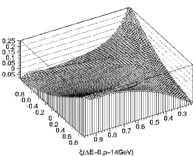
Figure 4.4: A three-dimensional plot of $\xi$ as a function of $2E_{l}/m_{t}$ ($x$-axis) and $\cos\theta_{te}$ ($y$-axis).

One can see that $\xi$ takes comparatively large positive values for either “small $E_{l}$ and $\cos\theta_{lt}\simeq-1$” or “large $E_{l}$ and $\cos\theta_{lt}\simeq+1$”. Oppositely, in the other two corners of the $E_{l}$–$\cos\theta_{lt}$ plane $\xi$ becomes negative. The typical magnitude of $\xi$ is 10–20%.

4.2.4 Measurements of Top Quark Couplings

As we have seen so far, studying various top quark properties in the $t\bar{t}$ threshold region is promising and interesting. Regarding the energy upgrading scenario of JLC, it is likely that the machine will operate first in the $t\bar{t}$ threshold region for a significant amount of time, while measuring the top quark mass precisely, etc., before the beam energies are increased to the open-top region. Therefore it is desirable that measurements of the various top quark couplings can be performed concurrently with other unique measurements near threshold, with sensitivities comparable to those in the open-top region.

Thus, systematic simulation studies on sensitivities to all the top quark couplings or the form factors in the $t\bar{t}$ threshold region are requested, which are not yet complete. Up to now, sensitivity studies in the threshold region were performed on the top quark width [5], on the top-Higgs Yukawa coupling [5, 18], as well as on the strong coupling constant $\alpha_{s}$. Also, there exists a theoretical study on the $CP$ violating couplings of the top quark. We review the present status of these studies below.

A) Measurements of $\Gamma_{t}$, $g_{tH}$, $\alpha_{s}$

Among various observables in the top quark threshold region, the height (normalization) of the $1S$ peak of the threshold cross section is most sensitive to the top quark decay width $\Gamma_{t}$, the top-Higgs Yukawa coupling $g_{tH}$, and the strong coupling constant $\alpha_{s}$. This is because: (1) according to Eq. (4.2), the peak height is inversely proportional to $\Gamma_{t}$ in the narrow width limit; (2) the effect of Higgs exchange enhances the cross section; (3) the wave function at origin $|\psi_{n}({\bf{0}})|^{2}$ is proportional to $\alpha_{s}^{3}$; when we take into account the smearing effect by the large decay width the sensitivity reduces to $\sim\alpha_{s}^{2}$. Nevertheless, extracting these quantities requires a precise theoretical prediction for the normalization of the threshold cross section. In view of the present large theoretical uncertainty, accurate measurements of $g_{tH}$ and $\alpha_{s}$ seem to be difficult, whereas we will still be able to measure $\Gamma_{t}$ relatively accurately. Also, the top momentum distribution and forward-backward asymmetry of the top quark depend on $\Gamma_{t}$ and $\alpha_{s}$. Theoretical predictions for these observables are expected to be more stable, but some more calculations are needed for accurate predictions.

Total $t\bar{t}$ Cross Section

Let us first discuss the results of the simulation studies, which set a benchmark of measurements in future experiments.

It is well known that the initial state radiation has to be properly taken into account in the vicinity of a resonance state. Also, in order to study experimental feasibilities in a realistic environment, we need to include the effects due to the beam energy spread and beamstrahlung (a bremsstrahlung from beam particles due to the strong electromagnetic fields produced by opposing beam bunches). These effects can be incorporated by convoluting the original cross section with the radiator function and the beam spectrum. The beam spectrum is machine dependent, and in our study below we use the parameters given in [5].

The effects on the cross section can be summarized as follows (see Figs. 4.5). (i) The initial state radiation and the beamstrahlung reduce usable luminosity in the threshold region. The usable part is essentially restricted to the $\delta$-function part of the beam spectrum. Therefore, we need to know the height of the $\delta$-function part accurately for precision measurements. (ii) The beam energy spread is the major source of the peak smearing. When the energy spread is less than 0.4%, the cross section shape is practically independent of the structure inside the $\delta$-function part. If we cannot achieve such a narrow band beam, it is important to measure the spectrum inside the $\delta$-function part with a high-energy resolution.

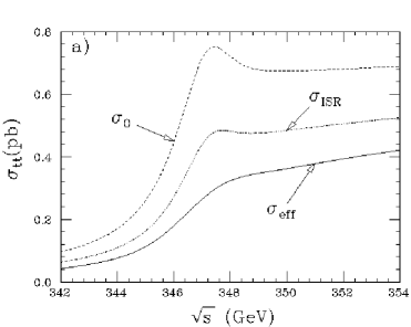
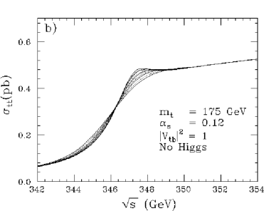
Figure 4.5: (a) Effects of the initial state radiation (ISR) and the beam energy spread and beamstrahlung on the threshold shape for $m_{t}=175$ GeV and $\alpha_{s}(M_{Z})=0.12$: with no ISR and no beam effects (dash), with ISR but without beam effects (dotdash), and with both ISR and beam effects (solid). (b) Threshold cross section including the effects of ISR and natural beam energy spread but leaving out the effect of beamstrahlung. Two kinds of spectra, flat-top (dot) and double-peaked (solid), which is more realistic, are examined for various beam energy spread: 0.1%, 0.4%, 0.7%, 1.0%, 1.4%.

The signature of a $t\bar{t}$ pair production is two $b$ quarks and two $W$ bosons in the final state. The two $W$ bosons decay into either $q\bar{q}^{\prime}$ or $\ell\nu$. Therefore the final state configurations are (i) two $b$ jets and four jets from $W$’s (45%), (ii) two $b$ jets, two jets, and one charged lepton (44%), and (iii) two $b$ jets and two charged leptons (11%). All three cases can be used for the measurement of the total cross section. Case (i) and (ii) are useful for the measurements of the top momentum distribution and top quark forward-backward asymmetry. The basic cuts used in the event selection can be classified into four groups: (a) event shape cuts such as those on the number of charged particles, the number of jets, and thrust, (b) mass cuts to select $W$’s and $t$’s by jet-invariant-mass method, (c) requirements of leptons in cases (ii) and (iii), and (d) $b$ taggings.

In order to measure the total $t\bar{t}$ cross section reliably, we need to select $t\bar{t}$ events with a good signal-to-background ratio. The largest background comes from $W^{+}W^{-}$ pair productions, whose cross section is larger by a factor $\sim 10^{3}$. We take case (i) as an example and show the result of a Monte Carlo simulation study. We require 20 or more charged tracks and impose cuts on the visible energy (the energy sum of all the detected particles including neutral ones) and the total transverse momentum: $E_{\rm vis}\geq 250$ GeV and $p_{T}\leq 50$ GeV. The remaining events must contain six or more hadronic jets after jet clustering with $y_{\rm cut}=5\times 10^{-3}$, where $y_{\rm cut}$ is the cut on jet-invariant-masses normalized by the visible energy. If there are more than six jets, we increase the $y_{\rm cut}$ value so as to make the event yield exactly six jets. Two pairs of jets out of these six jets must have 2-jet invariant masses consistent with $M_{W}$. These two $W$ candidates are then required to make invariant masses consistent with $m_{t}$, when combined with one of the remaining two jets. Finally we impose a cut on the event thrust: ${\rm thrust}\leq 0.75$. After the final cut, the detection efficiency is 29%, while the signal-to-background ratio is greater than 10. This detection efficiency translates to about 63% when the branching ratio for $W\to q\bar{q}^{\prime}$ of 67% is taken into account. We can select events with similar efficiencies and signal-to-background ratios for cases (ii) and (iii) as well.

Using the $t\bar{t}$ samples so obtained, we can determine the parameters $\Gamma_{t}$, $g_{tH}$, $\alpha_{s}$. 11 points with 1 fb^-1 each were generated with the inputs $m_{t,{\rm pole}}=170$ GeV, $\alpha_{s}(M_{Z})=0.12$, $m_{H}=\infty$ (no Higgs effects) and the SM value for $\Gamma_{t}$. By fitting these data points to the theoretical prediction for the total $t\bar{t}$ production cross section, convoluted with the beam spectrum, we obtained the following estimates of the statistical errors on the above parameters: $\Delta\Gamma_{t}/\Gamma_{t}^{\rm SM}=0.18$, $\Delta g_{tH}/g_{tH}^{\rm SM}=0.3$ in the case $M_{H}=115$ GeV, and $\Delta\alpha_{s}(M_{Z})=0.002$. Each error is given for a measurement of each parameter, assuming that the other parameters are known from other sources.

While the above errors serve as measures for potential sensitivities of the threshold measurements, as long as the theoretical uncertainty on the normalization of the cross section remains at the present level, theoretical errors on these parameters can be much larger. For example, the induced theoretical error on the strong coupling constant is $\Delta\alpha_{s}(M_{Z})\simeq 0.01$. As for $\Gamma_{t}$, we may consider a strategy to determine it to a good accuracy, nonetheless. Since the effect of the variation of $\Gamma_{t}$ appears only in the vicinity of the $1S$ peak (see Fig. 4.6), we may use, for instance, the ratio of the $t\bar{t}$ total cross section at $\sqrt{s}\simeq M_{1S}$ and at $\sqrt{s}\simeq M_{1S}+3$ GeV. This ratio is much less affected by the normalization uncertainty, and the statistical error on $\Delta\Gamma_{t}/\Gamma_{t}$ will be determined by the luminosity we invest at $\sqrt{s}\simeq M_{1S}$ and $\sqrt{s}\simeq M_{1S}+3$ GeV. We expect that an accuracy better than 15% (both theoretical and statistical) would be achievable with a moderate integrated luminosity.

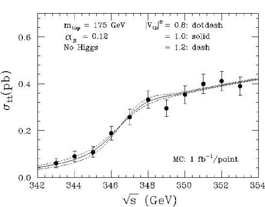
Figure 4.6: The dependence of the cross section as $\Gamma_{t}\propto|V_{tb}|^{2}$ is varied. An example of energy scan is superimposed, where each point corresponds to 1 fb^-1.

On the other hand, extraction of the Yukawa coupling requires, at the present status, a more accurate theoretical prediction. This is because its effect is to enhance the cross section almost energy independently in the threshold region, and disentanglement from the normalization uncertainty is difficult. To match the above statistical accuracy of the Yukawa coupling, the theoretical accuracy should become smaller than 4%. For the same reason, a precise measurement of $\alpha_{s}$ will also be difficult. A better strategy would be to determine the value of $\alpha_{s}(M_{Z})$ in other experiments and to use it as an input of the theoretical predictions in the top quark threshold region.

Top Momentum Distribution

By virtue of the large top quark width, we can measure the top quark momentum by reconstructing the 3-jet decay of a top quark, even below the $t\bar{t}$ threshold. This is in contrast to the charmonium and bottomonium cases, where the annihilation modes dominate. We assume that the program of JLC is such that the machine first scans the threshold shape with a relatively low integrated luminosity and determines the top quark mass accurately, then the c.m. energy is fixed at some point in the threshold region and we invest more luminosity to perform the measurements of the top momentum distribution, etc. The choice of the c.m. energy should be made from the viewpoint of insensitivity to theoretical ambiguities and beam effects and of sensitivities to physical parameters to be determined. Since the momentum distribution depends heavily on the c.m. energy, the initial state radiation and beam effects must be properly taken into account. From the study in [5], we find that the position of the peak momentum $|{\bf{p}}|_{\rm peak}$ is fairly stable against these effects, although the distribution itself is quite affected. An optimal c.m. energy, which maximizes the sensitivity to $\alpha_{s}(M_{Z})$ and $\Gamma_{t}$, while keeping small the beam effects and theoretical uncertainties, is chosen as 2 GeV above the 1S peak energy, $\Delta E\equiv\sqrt{s}-M_{1S}=2$ GeV. For simplicity, we assume that $M_{1S}$ is known in what follows.

In order to measure the top momentum, we need to select top quarks which are well-reconstructed as 3-jet systems from $t\to bW$ decays. This requires final states with at least one $t$ or $\bar{t}$ quark decaying into three jets: the configurations (i) and (ii) discussed above. The 6-jet mode [case (i)] is advantageous from the statistical point of view, since both $t$ and $\bar{t}$ quarks in a single event can be used for the momentum measurement. This mode, however, tends to suffer from combinatorial background: even if we have a perfect $b$-tagging capability, some ambiguity would still remain in assigning other four jets to two $W$’s. The lepton-plus-4-jet mode [case (ii)] is cleaner in this respect.

The selection of top quark events goes similarly to the one discussed in the total cross section analysis. In the present case, however, we have to make sure that the momentum of a reconstructed top quark is well measured. Rejection of events with energetic missing neutrinos is thus necessary. The main differences are the cut values which must be much tighter to require four-momentum balance, well reconstructed $W$’s and $t$’s. The $b$ tagging and the cut on the $b$-$W$ angle are necessary in addition. (See [5] for details.) In case (ii) Monte Carlo simulations resulted in a detection efficiency of 4% including the branching fraction to the lepton-plus-4-jet mode. The systematic shift between the peak momentum of the generated events and that of the reconstructed events is less than 1 GeV. The momentum resolution is 3–4 GeV in the relevant range, which is much smaller than the width of the momentum distribution. In case (i) the detection efficiency is 2%, including the branching fraction to the 6-jet mode. Since both $t$ and $\bar{t}$ can be used for the momentum measurement, effective selection efficiency is twice this value. The agreement of the reconstructed momentum distribution with the generated one is not as good as in the lepton-plus-4-jet case, because of the combinatorial background. A further study to gain in the detection efficiency using a kinematical fitting procedure is now underway.

We can estimate the statistical error on $|{\bf{p}}|_{\rm peak}$ from the width of the expected momentum distribution and the expected number of reconstructed top quarks. Using the events reconstructed from the lepton-plus-4-jet mode at $\Delta E=2$ GeV with $m_{t,{\rm pole}}=170$ GeV, the $1\sigma$ bound corresponding to an integrated luminosity of 100 fb^-1 is $\Delta|{\bf{p}}|_{\rm peak}\simeq 200$ MeV. This value translates to sensitivities to $\Gamma_{t}$ and $\alpha_{s}(M_{Z})$ of $\Delta\Gamma_{t}/\Gamma_{t}=0.03$ and $\Delta\alpha_{s}(M_{Z})=0.002$, when each parameter is varied while the other is fixed and assuming $M_{1S}$ is known.

Forward-Backward Asymmetry

As we have seen in Subsection 4.2.3, interference of the $S$- and $P$-wave resonances produces a forward-backward asymmetry of the top quark. The spectrum of the would-be toponium resonances is such that the lowest-lying $S$-wave resonance ($1S$ state) stands alone, while the higher $S$-wave resonances are accompanied by nearly degenerate $P$-wave resonances. The level spacings are determined by $\alpha_{s}$ while the resonance widths are determined mainly by the top quark width. The relative size of the two determines the size of the interference. Therefore, we expect that the forward-backward asymmetry provides additional information on the top quark width.

The c.m. energy is chosen in the same strategy as in the momentum distribution measurement. The asymmetry depends fairly strongly on the c.m. energy. As a consequence, the beam effects are sizable in the entire threshold region, and a good understanding or control of these effects will be mandatory in the asymmetry measurement. In consideration of the sensitivity to $\Gamma_{t}$, we chose the c.m. energy as $\Delta E=1$ GeV. Since the asymmetry is quite small, the systematic error due to the detector asymmetry must be carefully studied in actual experiments. We expect collider operations at the $Z$ pole (Giga $Z$) will be very useful, since the experimental limit on the measurable asymmetry will be determined by the number of events available for the detector calibration. We assume that a sample of 40,000 reconstructed events is given and estimate the expected statistical errors on $\alpha_{s}$ and $\Gamma_{t}$. The sample corresponds to 200 fb^-1 even if the detection efficiency is as high as 40%. For $m_{t,{\rm pole}}=170$ GeV, the sensitivity to the strong coupling constant is $\Delta\alpha_{s}(M_{Z})=0.004$ if $M_{1S}$ and $\Gamma_{t}$ are known. On the other hand, the sensitivity to the top quark width is $\Delta\Gamma_{t}/\Gamma_{t}=0.06$ if $M_{1S}$ and $\alpha_{s}(M_{Z})$ are known.

B) $CP$ Violating Couplings

Here, we review the recent theoretical study on probing the anomalous $CP$ violating interactions of the top quark in the threshold region [21]. Besides its own interest, it also serves as a case study for the analyses of top quark properties using its production-decay chain.

Among various interactions of the top quark, testing the CP-violating interactions is particularly interesting due to following reasons:

• Within the SM, CP-violation in the top quark sector is extremely small. If any CP-violating effect is detected in the top quark sector in a near-future experiment, it immediately signals new physics.

• There can be many sources of CP-violation in models that extend the SM. Besides, the observed baryon asymmetry in the Universe suggests existence of CP violating mechanisms beyond the SM.

• In relatively wide class of models beyond the SM, CP violation emerges especially sizably in the top quark sector.

In this analysis we consider CP-violating interactions of top quark with $\gamma$, $Z$, and $g$. In particular, we consider the lowest dimension CP-odd effective operators:

$${\cal L}_{\mbox{\scriptsize{\it CP}-odd}} = -\frac{ed_{t\gamma}}{2m_{t}}(\bar{t}i\sigma^{\mu\nu}\gamma_{5}t)\partial_{\mu}A_{\nu}-\frac{g_{Z}d_{tZ}}{2m_{t}}(\bar{t}i\sigma^{\mu\nu}\gamma_{5}t)\partial_{\mu}Z_{\nu}$$ (4.10)

$$-\frac{g_{s}d_{tg}}{2m_{t}}(\bar{t}i\sigma^{\mu\nu}\gamma_{5}T^{a}t)\partial_{\mu}G_{\nu}^{a},~{}~{}~{}~{}~{}~{}\sigma^{\mu\nu}\equiv{\textstyle\frac{i}{2}}[\gamma^{\mu},\gamma^{\nu}],$$

where $e=g_{W}\sin\theta_{W}$ and $g_{Z}={g_{W}}/{\cos\theta_{W}}$. These represent the interactions of $\gamma$, $Z$, $g$ with the EDM, $Z$-EDM, chromo-EDM of top quark, respectively. As stated, the SM contributions to these couplings are extremely small, $d_{t\gamma}^{\rm(SM)},d_{tZ}^{\rm(SM)},d_{tg}^{\rm(SM)}\sim 10^{-14}$. Our concern is in the anomalous couplings which are induced from some new physics. We assume that generally the couplings $d_{t\gamma}$, $d_{tZ}$, $d_{tg}$ are complex.

Which CP-odd observables are sensitive to the CP-violating couplings $d_{t\gamma}$, $d_{tZ}$, $d_{tg}$? For the process $e^{+}e^{-}\to t\bar{t}$, we may conceive of the following expectation values of kinematical variables for CP-odd observables:

$$\left<\,({\bf{p}}_{e}-\bar{{\bf{p}}}_{e})\cdot({\bf{s}}_{t}-\bar{{\bf{s}}}_{t})\,\right>,$$

$$\left<\,({\bf{p}}_{t}-\bar{{\bf{p}}}_{t})\cdot({\bf{s}}_{t}-\bar{{\bf{s}}}_{t})\,\right>,$$ (4.11)

$$\left<\,[({\bf{p}}_{e}-\bar{{\bf{p}}}_{e})\times({\bf{p}}_{t}-\bar{{\bf{p}}}_{t})]\cdot({\bf{s}}_{t}-\bar{{\bf{s}}}_{t})\,\right>,$$

where the spins and momenta are defined in the c.m. frame. The above quantities are the three components of the difference of the $t$ and $\bar{t}$ spins. All the other CP-odd observables for $e^{+}e^{-}\to t\bar{t}$ are bilinear in ${\bf{s}}_{t}$ and $\bar{{\bf{s}}}_{t}$. Since analyses of spin correlations are complicated, we focus on the difference of the polarization vectors.

Practically we can measure the $t$ and $\bar{t}$ polarization vectors efficiently using $\ell^{\pm}$ angular distributions. It is known that the angular distribution of the charged lepton $\ell^{+}$ from the decay of top quark is maximally sensitive to the top quark polarization vector. In the rest frame of top quark, the $\ell^{+}$ angular distribution is given by [15]

$$\frac{1}{\Gamma_{t}}\,\frac{d\Gamma(t\to b\ell^{+}\nu)}{d\cos\theta_{\ell^{+}}}=\frac{1+S\cos\theta_{\ell^{+}}}{2}$$ (4.12)

at tree level, where $S$ is the top quark polarization and $\theta_{\ell^{+}}$ is the angle of $\ell^{+}$ measured from the direction of the top quark polarization vector, cf. Eq. (4.4). Indeed the $\ell^{+}$ distribution is ideal for extracting CP-violation in the $t\bar{t}$ production process; the above angular distribution is unchanged even if anomalous interactions are included in the $tbW$ decay vertex, up to the terms linear in the decay anomalous couplings and within the approximation $m_{b}=0$ [37]. Therefore, if we consider the average of the lepton direction, for instance, we may extract the top quark polarization vector efficiently:

$$\left<{\bf{n}}\cdot{\bf{n}}_{\ell}\right>_{\rm Lab}\simeq\frac{1}{3}\,{\bf{n}}\cdot{\bf{S}}.$$ (4.13)

The average is to be taken at the top quark rest frame, but in the threshold region, we may take the average in the laboratory frame barely without loss of sensitivities to the anomalous couplings.

From rough estimates, we estimated the statistical errors to the anomalous CP-violating couplings of the top quark with $\gamma$, $Z$ and $g$ in the $t\bar{t}$ threshold region: $\delta d_{t\gamma}$, $\delta d_{tZ}$, $\delta d_{tg}\sim 10\%$ corresponding to an integrated luminosity of 50 fb^-1. In Table 4.1 we summarize the results of the sensitivity studies performed so far, including the results of our present study.

Table 4.1: The results of studies of sensitivities to the anomalous couplings expected in future experiments. For $e^{+}e^{-}$ linear colliders (LC), “open top” denotes the results of studies performed at $\sqrt{s}=500$ GeV.

		$\delta d_{tg}$	$\delta d_{t\gamma}$	$\delta d_{tZ}$
LHC     (10 fb-1)		$10^{-2}$ – a few$\times 10^{-3}$	-	-
$e^{+}e^{-}$ LC	open top	${\cal O}(1)$	$10^{-1}$ – a few$\times 10^{-2}$	$10^{-1}$ – a few$\times 10^{-2}$
(50 fb-1)	$t\bar{t}$ threshold	$10^{-1}$	$10^{-1}$	$10^{-1}$

We may compare the sensitivities of experiments in the $t\bar{t}$ threshold region at $e^{+}e^{-}$ colliders (JLC) with others. The sensitivities to $d_{t\gamma}$ and $d_{tZ}$ are comparable to those attainable in the open-top region at $e^{+}e^{-}$ colliders. The sensitivity to $d_{tg}$ is worse than that expected at a hadron collider but exceeds the sensitivity in the open-top region at $e^{+}e^{-}$ colliders. (It should be noted, however, that although a hadron collider has a high sensitivity to this quantity, accuracy of its measurement is not very good, and vice versa for $e^{+}e^{-}$ colliders.)

Qualitatively, the characteristics of the $t\bar{t}$ region are summarized as follows.

1. We can measure the three couplings $d_{t\gamma}$, $d_{tZ}$, $d_{tg}$ simultaneously and we can disentangle each contribution.

2. Typical sizes of components of the difference of the $t$ and $\bar{t}$ polarizations are given by

   $$|\delta{S}_{\perp}|,\,|\delta{S}_{\rm N}|\sim(\mbox{5--20}\%)\times(d_{t\gamma},d_{tZ},d_{tg}).$$

   They can be extracted efficiently from the directions of charged leptons from decays of $t$ and $\bar{t}$:

   $$\langle\langle{\bf{n}}\cdot({\bf{n}}_{\ell}+\bar{{\bf{n}}}_{\ell})\rangle\rangle_{{\bf{p}}_{t}}\simeq\frac{2}{3}\,{\bf{n}}\cdot\delta{\bf{S}}.$$

3. We can measure the complex phases of the couplings $d_{t\gamma}$, $d_{tZ}$, $d_{tg}$. Since the strong phases can be modulated at our disposal, a single observable ($\delta{S}_{\perp}$ or $\delta{S}_{\rm N}$) probes the phases of the couplings.

We note that if one of the couplings is detected in the future, we would certainly want to measure the others in order to gain deeper understanding of the CP-violating mechanism. This is because one may readily think of various underlying processes which give different contributions to the individual couplings.

Regarding (1) and (2) above, QCD interaction is used as a controllable tool for the detection of the anomalous couplings. This would be the first trial to use QCD interaction for such a purpose without requiring any phenomenological inputs.

4.3 Top Quark Mass Measurement from $t\bar{t}$ Dilepton events

The top quark mass can also be determined from direct reconstruction of

$$t\bar{t}\rightarrow W^{+}bW^{-}\bar{b}\rightarrow\ell^{+}\ell^{-}\nu\bar{\nu}b\bar{b}$$

Dilepton events at JLC, in addition to the mass determination from the $t\bar{t}$ threshold scan. CDF and D0 have determined the top quark mass to be $174.3\pm 5.1$ GeV/c² from direct reconstruction of $t\bar{t}$ events. The top quark mass is expected to be determined to a precision of 1 to 2 GeV/c² at the Tevatron and the LHC. For direct reconstruction, the Dilepton channel has the smallest systematic uncertainty, in comparison with the Lepton + Jets and Multi-jet channels. In contrast to the hadron colliders, the beam energy at the Linear Collider provides constraints in the kinematic reconstruction. A precision of 200 MeV/c² on the top quark mass can be achieved at JLC [22].

4.4 Measurement of Top-Yukawa Coupling

4.4.1 Theoretical Background

At higher energies, where $e^{+}e^{-}\to t\bar{t}H$ is open, we can carry out a more direct measurement of the top Yukawa coupling. There are two kinds of diagrams to the $e^{+}e^{-}\to t\bar{t}H$ process at the tree level. The first kind includes diagrams where a Higgs boson is radiated off the final-state top or anti-top legs ($H$-off-$t$) and is thus proportional to the top Yukawa coupling. The second kind consists of the one with a Higgs boson from the $s$-channel $Z$ ($H$-off-$Z$) and is independent of the top Yukawa coupling.

Figures 4.7-a) and -b) plot the contributions of these two kinds of diagrams in terms of the production cross section for (a) $m_{H}=100~{}{\rm GeV}$ and (b) $m_{H}=150~{}{\rm GeV}$. The cross sections are calculated for $m_{t}=170~{}{\rm GeV}$ with the initial state radiation but without beam effects which are heavily machine-dependent. The key point here is that the $H$-off-$t$ diagrams dominate the $H$-off-$Z$ diagram, so that the total cross section is essentially proportional to $\beta_{H}^{2}$. A simple counting experiment thus serves as a direct top Yukawa coupling measurement.

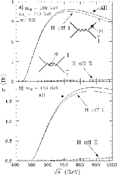
Figure 4.7: The production cross sections for $e^{+}e^{-}\to t\bar{t}H$ with $m_{t}=170~{}{\rm GeV}$ as functions of $\sqrt{s}$: (a) $m_{H}=100~{}{\rm GeV}$ and (b) $m_{H}=150~{}{\rm GeV}$, both with initial state radiation, leaving out the beam effects. The dot-dashed lines are the contributions from the $H$-off-$t$ diagrams (signal diagrams), while the dashed lines are from the $H$-off-$Z$ diagram (background).

4.4.2 Event Selection

The question is how well we can separate signal from background, since the production cross section is not very large. The signal for $t\bar{t}H$ production is 2 $W$’s and 4 $b$’s, where the $W$’s decay into either $q\bar{q}^{\prime}$ or $l\nu$. Depending on how the two $W$’s decay, we have three modes: (1) 8 jets (38%), (2) a lepton plus 6 jets (37 %), and two leptons + 4 jets (the rest). Here, we consider the modes (1) and (2). The background, on the other hand, can be classified into two groups: (i) irreducible ones containing the $e^{+}e^{-}\to t\bar{t}Z$ followed by $Z\to b\bar{b}$ (separable if $m_{H}$ is far from $m_{Z}$) and the $H$-off-$Z$ diagram which is tiny, (ii) reducible ones of which the biggest is $e^{+}e^{-}\to t\bar{t}$ with gluon emissions.

Basic cuts to select signal events from the background consist of event shape cuts requiring 8 or 6 jets in the final state and small thrust (e.g. thrust $<0.8$), mass cuts demanding $m_{2J}\simeq m_{W}/m_{H}$ and $m_{3J}\simeq m_{t}$, and, in the case of the 8-jet mode, four-momentum balance: $P_{T}<50~{}{\rm GeV}$ and $\Delta E_{vis}<200~{}{\rm GeV}$. In addition, the $b$-tagging requiring more than two $b$-jet candidates in the final state is crucial. Here, we conservatively assume the base-line JLC-I values for the tagging efficiencys: $\epsilon_{b}=0.78$ and $\epsilon_{c}=0.38$. The resultant signal-to-noise ratio heavily depends on the $b$-tagging performance as well as on the Higgs mass which controls the background from the $e^{+}e^{-}\to t\bar{t}Z$ process.

In order to study the event selection feasibility, we have generated the $t\bar{t}H$ events and the $t\bar{t}$ and $t\bar{t}Z$ background events for $m_{t}=170~{}{\rm GeV}$ and $m_{H}=100~{}{\rm GeV}$ at $\sqrt{s}=700~{}{\rm GeV}$, with the beam width and beamstrahlung as given in Ref.[35]. These events were fed into the JLC-I detector simulator[35] and processed through the event selection described above. Scatter plots of 2-jet invariant masses for $W$ and $H$ candidates in the signal events after the above selection is shown in Figs. 4.8-a) and -b) for the 8-jet and the lepton-plus-6-jet modes, respectively.

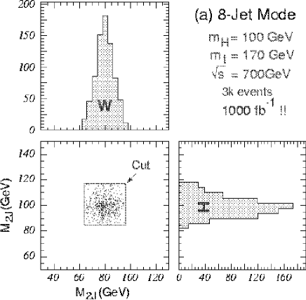
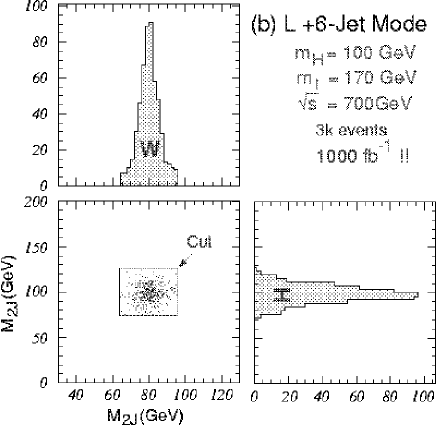
Figure 4.8: A scatter plot of 2-jet invariant masses for $W$ and $H$ candidates in the signal events shown together with its projection to the two axes: (a) 8-jet mode and (b) lepton-plus-6-jet mode.

Next we discuss the S/N ratio. Figs. 4.9-a) and -b) are the thrust distributions for the signal ($t\bar{t}H$) and the background ($t\bar{t}$) events for the 8-jet and lepton-plus-6-jet modes, respectively.

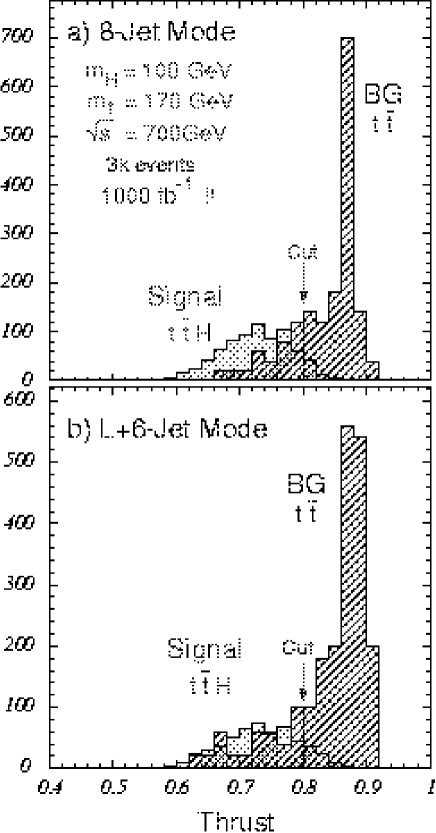
Figure 4.9: Thrust distributions for the signal $t\bar{t}H$ (solid) and the background $t\bar{t}$ (hatched) events: (a) 8-jet mode and (b) lepton-plus-6-jet mode.

We can see that the signal events are more spherical than the background and consequently have smaller thrusts. The cut at 0.8 thus removes the background very effectively. Nevertheless, the $t\bar{t}$ background is still large even after the rather tight selection described above. The situation can be improved significantly by the use of a better vertex detector: in principle, the requirement of more than two $b$-jets in the final state reduces the $t\bar{t}$ background to a negligible level, as long as the $b$-purity is near 100%.

We will, however, assume this S/N ratio and examine the sensitivity to the top Yukawa coupling in this conservative case.

4.4.3 Determination of Top Yukawa Coupling

With the initial state radiation and beam effects, the signal cross section at $\sqrt{s}=700~{}{\rm GeV}$ for $m_{t}=170~{}{\rm GeV}$ and $m_{H}=100~{}{\rm GeV}$ is $\sigma_{t\bar{t}H}\simeq 3.0~{}{\rm fb}$. The overall selection efficiencies for the 8-jet and the lepton-plus-6-jet modes are 0.23 and 0.16, respectively, including the branching fractions. The total selection efficiency thus amounts to

$$\epsilon_{t\bar{t}H}=0.23+0.16=0.39.$$

On the other hand, the effective background cross sections are $\sigma_{t\bar{t}Z}\simeq 4.2~{}{\rm fb}$ and $\sigma_{t\bar{t}}\simeq 402~{}{\rm fb}$, including the initial state radiation and beam effects. The corresponding overall detection efficiencies for the background events are

$$\epsilon_{t\bar{t}Z}=0.088({\rm 8J})+0.048({\rm L+6J})=0.14$$

$$\epsilon_{t\bar{t}}=0.0009({\rm 8J})+0.0010({\rm L+6J})=0.0019.$$ (4.14)

The expected number of the signal events for $100~{}{\rm fb}^{-1}$ is $S=114$ while that for the background is $B=133$, resulting in a signal-to-noise ratio of 0.86. Making use of the fact that the number of the signal events is essentially proportional to the square of the normalized top Yukawa coupling ($\beta_{H}^{2}$), we can translate these numbers to the error on $\beta_{H}$: $\Delta\beta_{H}/\beta_{H}\simeq 0.14$ for $100~{}{\rm fb}^{-1}$ at $\sqrt{s}=700~{}{\rm GeV}$.

4.5 Probe for anomalous $t\bar{t}H$ couplings at JLC

In this section, we review the recent theoretical study on probing the anomalous $t\bar{t}H$ couplings in the process of the Higgs boson and top-quark associated production [23]

$$e^{+}e^{-}\to t\bar{t}H.$$ (4.15)

By scrutinizing this process in detail, one would hope to reveal the nature of the Higgs and top-quark interactions and hopefully gain some insight for physics beyond the SM.

4.5.1 Effective Interactions

As a model-independent approach, anomalous couplings of the top quark can be parameterized by a low-energy effective Lagrangian. Such an approach has been taken in Ref. [24] in a non-linear realization of the gauge symmetry, and in Refs. [25, 26] in a linear realization with an explicit scalar (Higgs boson) field.

In the latter case, the anomalous couplings are parameterized by a set of higher dimensional operators which contain the SM fields and are invariant under the SM gauge group, $SU_{c}(3)\times SU_{L}(2)\times U_{Y}(1)$. Below the new physics scale $\Lambda$, the effective Lagrangian can be written as

$${\cal L}_{eff}={\cal L}_{0}+\frac{1}{\Lambda^{2}}\sum_{i}C_{i}O_{i}+{\cal O}(\frac{1}{\Lambda^{4}})$$ (4.16)

where $\Lambda$ is a cutoff scale above which new physics sets in, and ${\cal L}_{0}$ is the SM Lagrangian. $O_{i}$ are dimension-six operators and $C_{i}$ represent the coupling strengths of $O_{i}$ [25].

Following Refs. [26, 27], we find that there are seven dimension-six CP-even operators which give new contributions to the couplings of $H$ to the top quark,

$$O_{t1} = (\Phi^{\dagger}\Phi-\frac{v^{2}}{2})\left[\bar{q}_{L}t_{R}\widetilde{\Phi}+\widetilde{\Phi}^{\dagger}\bar{t}_{R}q_{L}\right],$$ (4.17)

$$O_{t2} = i\left[\Phi^{\dagger}D_{\mu}\Phi-(D_{\mu}\Phi)^{\dagger}\Phi\right]\bar{t}_{R}\gamma^{\mu}t_{R},$$ (4.18)

$$O_{Dt} = (\bar{q}_{L}D_{\mu}t_{R})D^{\mu}\widetilde{\Phi}+(D^{\mu}\widetilde{\Phi})^{\dagger}(\overline{D_{\mu}t_{R}}q_{L}),$$ (4.19)

$$O_{tW\Phi} = \left[(\bar{q}_{L}\sigma^{\mu\nu}\tau^{I}t_{R})\widetilde{\Phi}+\widetilde{\Phi}^{\dagger}(\bar{t}_{R}\sigma^{\mu\nu}\tau^{I}q_{L})\right]W^{I}_{\mu\nu},$$ (4.20)

$$O_{tB\Phi} = \left[(\bar{q}_{L}\sigma^{\mu\nu}t_{R})\widetilde{\Phi}+\widetilde{\Phi}^{\dagger}(\bar{t}_{R}\sigma^{\mu\nu}q_{L})\right]B_{\mu\nu},$$ (4.21)

$$O_{\Phi q}^{(1)} = i\left[\Phi^{\dagger}D_{\mu}\Phi-(D_{\mu}\Phi)^{\dagger}\Phi\right]\bar{q}_{L}\gamma^{\mu}q_{L},$$ (4.22)

$$O_{\Phi q}^{(3)} = i\left[\Phi^{\dagger}\tau^{I}D_{\mu}\Phi-(D_{\mu}\Phi)^{\dagger}\tau^{I}\Phi\right]\bar{q}_{L}\gamma^{\mu}\tau^{I}q_{L},$$ (4.23)

where $\Phi$ is the Higgs doublet with $\widetilde{\Phi}=i\sigma_{2}\Phi^{*}$, and $\bar{q}_{L}=(\bar{t}_{L},\bar{b}_{L})$. Similarly, there are seven dimension-six CP-odd operators [28] which contribute to the couplings of $H$ to a top quark,

$$\overline{O}_{t1} = i(\Phi^{\dagger}\Phi-\frac{v^{2}}{2})\left[\bar{q}_{L}t_{R}\widetilde{\Phi}-\widetilde{\Phi}^{\dagger}\bar{t}_{R}q_{L}\right],$$ (4.24)

$$\overline{O}_{t2} = \left[\Phi^{\dagger}D_{\mu}\Phi+(D_{\mu}\Phi)^{\dagger}\Phi\right]\bar{t}_{R}\gamma^{\mu}t_{R},$$ (4.25)

$$\overline{O}_{Dt} = i\left[(\bar{q}_{L}D_{\mu}t_{R})D^{\mu}\widetilde{\Phi}-(D^{\mu}\widetilde{\Phi})^{\dagger}(\overline{D_{\mu}t_{R}}q_{L})\right],$$ (4.26)

$$\overline{O}_{tW\Phi} = i\left[(\bar{q}_{L}\sigma^{\mu\nu}\tau^{I}t_{R})\widetilde{\Phi}-\widetilde{\Phi}^{\dagger}(\bar{t}_{R}\sigma^{\mu\nu}\tau^{I}q_{L})\right]W^{I}_{\mu\nu},$$ (4.27)

$$\overline{O}_{tB\Phi} = i\left[(\bar{q}_{L}\sigma^{\mu\nu}t_{R})\widetilde{\Phi}-\widetilde{\Phi}^{\dagger}(\bar{t}_{R}\sigma^{\mu\nu}q_{L})\right]B_{\mu\nu},$$ (4.28)

$$\overline{O}_{\Phi q}^{(1)} = \left[\Phi^{\dagger}D_{\mu}\Phi+(D_{\mu}\Phi)^{\dagger}\Phi\right]\bar{q}_{L}\gamma^{\mu}q_{L},$$ (4.29)

$$\overline{O}_{\Phi q}^{(3)} = \left[\Phi^{\dagger}\tau^{I}D_{\mu}\Phi+(D_{\mu}\Phi)^{\dagger}\tau^{I}\Phi\right]\bar{q}_{L}\gamma^{\mu}\tau^{I}q_{L}.$$ (4.30)

Operators (4.17)$-$(4.30) contribute to both the three-point coupling $~{}t\bar{t}H~{}$ as well as four-point couplings $t\bar{t}HZ$ and $t\bar{t}H\gamma$ beyond the SM. Operators $O_{t1}$ and $\overline{O}_{t1}$ give the direct corrections to the top-quark Yukawa coupling and is energy-independent. Only $O_{Dt}$ and $\overline{O}_{Dt}$ contribute to both three-point and four-point couplings and the three-point couplings are quadratically dependent on energy, due to the nature of double-derivative couplings.

4.5.2 $t\bar{t}H$ Production with Non-standard Couplings

The relevant Feynman diagrams for $e^{+}e^{-}\to t\bar{t}H$ production are depicted in Fig. 4.10, where (a)$-$(c) are those in the SM and the dots denote the contribution from new interactions.

Figure 4.10: Feynman diagrams for $e^{+}e^{-}\to t\bar{t}H$ production. (a)-(c) are those in the SM. The dots denote the contribution from new interactions.

For the purpose of illustration, we will only present results for the operators $O_{t1}$ (energy-independent) and $O_{Dt}$ (most sensitive to energy scale) and hope that they are representative to the others with similar energy-dependence based on the power-counting behavior. For simplicity, we assume one operator to be non-zero at a time in our study.

In Fig. 4.11 we show the Higgs boson mass dependence of the cross section for $\sqrt{s}=500$ GeV. A few representative values of the couplings $C_{t1}$ and $C_{Dt}$ are illustrated. The thick solid curves are for the operator $O_{t1}$, while the thin solid ones are for $O_{Dt}$.

Figure 4.11: Total cross section for $e^{+}e^{-}\to t\bar{t}H$ production versus $m_{H}$ for $\sqrt{s}=500$ GeV. The dashed curves are for the SM expectation.

Fig. 4.12 shows the behavior of the cross sections as functions of the anomalous couplings.

Figure 4.12: Total cross section for $e^{+}e^{-}\to t\bar{t}H$ production versus the couplings (a) for $O_{t1}$ and (b) for $O_{Dt}$ at $\sqrt{s}=500$ GeV with $m_{H}=100,~{}120,~{}140$ GeV.

To establish the sensitivity limits on the non-standard couplings that may be probed at JLC experiments, one needs to consider the identification of the final state from $t\bar{t}H$, including the branching ratios and the detection efficiencies. For a light Higgs boson of current interest, its leading decay mode is $H\to b\bar{b}$. The branching ratio for this mode is about $80\%\sim 50\%$ for the mass range of $100\sim 130$ GeV. To assure a clear signal identification, we require to identify four $b$-jets in the final state. We assume a 65% efficiency for single $b$-tagging [31]. As for the decays of $W^{\pm}$ from $t\bar{t}$, to effectively increase the signal rate, we include both the leptonic decay ($e^{\pm},\mu^{\pm}$) [29] and the pure hadronic decay [30]. These amount to about 85% of the $t\bar{t}$ events. With the above event selection and imposing certain selective acceptance cuts, one expects to significantly suppress the QCD and EW background processes $e^{+}e^{-}\to gt\bar{t},\ Zt\bar{t}$ [29, 30]. We estimate an efficiency factor $\epsilon$ for detecting $e^{+}e^{-}\to t\bar{t}H$ to be

$$\epsilon=10-30\%,$$

and a factor $\epsilon^{\prime}$ for reducing QCD and EW background to be

$$\epsilon^{\prime}=10\%,$$

in our further evaluation. The background cross sections for QCD, electroweak and $e^{+}e^{-}\to t\bar{t}H$ in the SM at $\sqrt{s}=500$ GeV without branching ratios and cuts included are 0.84, 0.19, 0.38 $fb$ respectively for $m_{H}=120$ GeV, which are consistent with those in [30].

To estimate the luminosity ($L$) needed for probing the effects of the non-standard couplings, we define the significance of a signal rate ($S$) relative to a background rate ($B$) in terms of the Gaussian statistics,

$$\sigma_{S}={S\over\sqrt{B}},$$ (4.31)

for which a signal at 95% (99%) confidence level (C.L.) corresponds to $\sigma_{S}=2\ (3)$.

4.5.3 CP-even Operators

In the presence of the CP-even operators, the $t\bar{t}H$ cross section ($\sigma$) would be thus modified from the SM expectation. The event rates in Eq. (4.31) are calculated as

$$S=L(|\sigma-\sigma_{SM}|)\epsilon\ \ {\rm and}\ \ B=L\left[\sigma_{SM}\epsilon+(\sigma_{QCD}+\sigma_{EW})\epsilon^{\prime}\right].$$ (4.32)

We then obtain the luminosity required for observing the effects of $O_{t1}$ at 95% C.L. at 500 GeV, which is shown in Fig. 4.13, where the two curves are for 10% and 30% of signal detection efficiency, respectively. We see that at a 500 GeV collider, one would need a high integrated luminosity to reach the sensitivity to the non-standard couplings.

Figure 4.13: Sensitivity to the anomalous couplings $O_{t1}$ versus the integrated luminosity for a 95% confidence level limits at $\sqrt{s}=500$ GeV.

4.5.4 CP-odd Operators

If there exist effective CP-odd operators besides the SM interaction, then CP will be violated in the Higgs and top-quark sectors. Similarly to the discussion in the previous section, one can try to observe the effects of the operators beyond the SM.

To unambiguously establish the observation of CP violation, one needs to examine CP-violating observables. The CP-violating effect can be parameterized by a cross section asymmetry as

$$A_{CP}\equiv\frac{\sigma((p_{1}\times p_{3})\cdot p_{4}<0)-\sigma((p_{1}\times p_{3})\cdot p_{4}>0)}{\sigma((p_{1}\times p_{3})\cdot p_{4}<0)+\sigma((p_{1}\times p_{3})\cdot p_{4}>0)}$$ (4.33)

where $p_{1}$, $p_{3}$ and $p_{4}$ are the momenta of the incoming electron, top quark and anti-top quark, respectively. Unfortunately, it requires a higher luminosity to detect the CP-violating effects.

4.6 Probe for Anomalous $t\gamma$, $tZ$, $tW$ Couplings

The discovery of the top-quark completed the fermion list required in the standard EW theory (SM). However it is still an open question whether this quark interacts with the others the standard way or there exists any new-physics contribution to its couplings. It decays immediately after being produced because of the huge mass. Therefore this process is not influenced by any hadronization effects and consequently the decay products are expected to tell us a lot about parent top property.

Next linear colliders (NLC) of $e^{+}e^{-}$ will give us fruitful data on the top through $e^{+}e^{-}\to t\bar{t}$. In particular the final lepton(s) produced in its semileptonic decay(s) turns out to carry useful information of the top-quark couplings [36]. Indeed many authors have worked on this subject (see the reference list of Ref.[37]), and we also have tackled them over the past several years.

Here we would like to show some of the results of our latest model-independent analyses of the lepton distributions for arbitrary longitudinal beam polarizations [37], where we have assumed the most general anomalous couplings both in the production and decay vertices in contrast to most of the existing works. What we actually studied are the lepton angular-energy distribution and the angular distribution, both of which would enable us to perform interesting tests of the top-quark couplings.

4.6.1 Framework

We can represent the most general covariant $t\bar{t}$ couplings to the photon and $Z$ boson as

$${\mit\Gamma}_{vt\bar{t}}^{\mu}=\frac{g}{2}\,\bar{u}(p_{t})\,\Bigl{[}\,\gamma^{\mu}(A_{v}-B_{v}\gamma_{5})+\frac{(p_{t}-p_{\bar{t}})^{\mu}}{2m_{t}}(C_{v}-D_{v}\gamma_{5})\,\Bigr{]}\,v(p_{\bar{t}})$$ (4.34)

in the $m_{e}=0$ limit, where $g$ denotes the $SU(2)$ gauge coupling constant and $v=\gamma/Z$. Among the above form factors, $A_{\gamma,Z}$, $B_{\gamma,Z}$ and $C_{\gamma,Z}$ are parameterizing $C\!P$-conserving interactions, while $D_{\gamma,Z}$ is $C\!P$-violating one.

On the other hand, we adopted the following parameterization of the $tbW$ vertex suitable for the $t\to W^{+}b$ and $\bar{t}\to W^{-}\bar{b}$ decays:

$$\!\!{\mit\Gamma}^{\mu}_{Wtb}=-{g\over\sqrt{2}}\>\bar{u}(p_{b})\biggl{[}\,\gamma^{\mu}(f_{1}^{L}P_{L}+f_{1}^{R}P_{R})-{{i\sigma^{\mu\nu}k_{\nu}}\over M_{W}}(f_{2}^{L}P_{L}+f_{2}^{R}P_{R})\,\biggr{]}u(p_{t}),\ \ \ \ \ \$$ (4.35)

$$\!\!\bar{\mit\Gamma}^{\mu}_{Wtb}=-{g\over\sqrt{2}}\>\bar{v}(p_{\bar{t}})\biggl{[}\,\gamma^{\mu}(\bar{f}_{1}^{L}P_{L}+\bar{f}_{1}^{R}P_{R})-{{i\sigma^{\mu\nu}k_{\nu}}\over M_{W}}(\bar{f}_{2}^{L}P_{L}+\bar{f}_{2}^{R}P_{R})\,\biggr{]}v(p_{\bar{b}}),$$ (4.36)

where $k$ is the $W$-boson momentum and $P_{L/R}=(1\mp\gamma_{5})/2$. This is also the most general form as long as we treat $W$ as an on-mass-shell particle, which is indeed a good approximation. It is worth mentioning that these form factors satisfy $f_{1}^{L,R}=\pm\bar{f}_{1}^{L,R}$ and $f_{2}^{L,R}=\pm\bar{f}_{2}^{R,L}$, where upper (lower) signs are those for $C\!P$-conserving (-violating) contributions.

4.6.2 Angular-energy distributions

After some calculations, we arrived at the following angular-energy distribution of the final lepton:

$$\frac{d^{2}\sigma}{dxd\cos\theta}=\frac{3\pi\beta\alpha^{2}}{2s}B\>\Bigl{[}\>S^{(0)}(x,\theta)$$

$$\ \ \ \ \ \ +\!\!\sum_{v=\gamma,Z}\bigl{[}\>{\rm Re}(\delta\!A_{v}){\cal F}_{Av}(x,\theta)+{\rm Re}(\delta\!B_{v}){\cal F}_{Bv}(x,\theta)+{\rm Re}(\delta C_{v}){\cal F}_{Cv}(x,\theta)$$

$$\ \ \ \ \ \ \ \ \ \ \ +{\rm Re}(\delta\!D_{v}){\cal F}_{Dv}(x,\theta)\>\bigr{]}+{\rm Re}(f^{R}_{2}){\cal F}_{2R}(x,\theta)\>\Bigr{]},$$ (4.37)

where $\beta\>(\equiv\sqrt{1-4m_{t}^{2}/s})$ is the top-quark velocity, $B$ denotes the appropriate branching fraction (=0.22 for $e/\mu$), $x$ means the normalized energy of $\ell$ defined in terms of its energy $E$ as $x\equiv 2E\sqrt{(1-\beta)/(1+\beta)}/m_{t}$, $\theta$ is the angle between the $e^{-}$ beam direction and the $\ell$ momentum, all in the $e^{+}e^{-}$ CM frame, $S^{(0)}$ is the SM contribution, $\delta\!A_{v}\sim\delta\!D_{v}$ express non-SM part of $A_{v}\sim D_{v}$ (i.e., $\delta\!B_{\gamma}$, $\delta C_{v}$ and $\delta\!D_{v}$ are equivalent respectively to $B_{\gamma}$, $C_{v}$ and $D_{v}$), and ${\cal F}$ are all analytically-expressed functions of $x$ and $\theta$, which are independent of each other. A similar formula also holds for the final $b$-quark.

Equation (4.37) can be re-expressed as

$$\frac{d^{2}\sigma}{dxd\cos\theta}=\frac{3\pi\beta\alpha^{2}}{2s}B\>\Bigl{[}\>{\mit\Theta}_{0}(x)+\cos\theta\,{\mit\Theta}_{1}(x)+\cos^{2}\theta\,{\mit\Theta}_{2}(x)\>\Bigr{]}.$$ (4.38)

This form directly leads to the angular distribution for $\ell$ through the integration over $x$:

$$\frac{d\sigma}{d\cos\theta}=\int_{x_{-}}^{x_{+}}dx\frac{d^{2}\sigma}{dxd\cos\theta}=\frac{3\pi\beta\alpha^{2}}{2s}B\left({\mit\Omega}_{0}+{\mit\Omega}_{1}\cos\theta+{\mit\Omega}_{2}\cos^{2}\theta\right),$$ (4.39)

where ${\mit\Omega}_{0,1,2}\equiv\int_{x_{-}}^{x_{+}}dx\,{\mit\Theta}_{0,1,2}(x)$ and $x_{\pm}$ define the kinematical range of $x$.

Surprisingly enough, the non-SM decay part, i.e., $f^{R}_{2}$ term completely disappears through this $x$ integration, and the angular distribution depends only on the whole production vertex plus the SM decay vertex [37, 38]. This never happens in the final $b$-quark distribution.

4.6.3 Analyzing the results

First, we could determine $\delta\!A_{v}\sim\delta\!D_{v}$ and $f^{R}_{2}$ simultaneously using the angular-energy distribution (4.37) via the optimal-observable procedure [39], since these anomalous parameters are all coefficients of independent functions. In the second paper of Ref.[37], we explored the best $e^{\pm}$ polarizations which minimize the expected statistical uncertainty ($1\sigma$) for each parameter.

On the other hand, we can perform another interesting test via the angular distribution. That is, asymmetries like

$${\cal A}_{\scriptscriptstyle{C\!P}}(\theta)=\Big{[}\>{\displaystyle\frac{d\sigma^{+}(\theta)}{d\cos\theta}-\frac{d\sigma^{-}(\pi-\theta)}{d\cos\theta}}\>\Bigr{]}\Big{/}\Bigl{[}\>{\displaystyle\frac{d\sigma^{+}(\theta)}{d\cos\theta}+\frac{d\sigma^{-}(\pi-\theta)}{d\cos\theta}}\>\Bigr{]}$$ (4.40)

or

$${\cal A}_{\scriptscriptstyle{C\!P}}=\frac{{\displaystyle\int_{-c_{m}}^{0}\!d\cos\theta\frac{d\sigma^{+}(\theta)}{d\cos\theta}-\int_{0}^{+c_{m}}\!d\cos\theta\frac{d\sigma^{-}(\theta)}{d\cos\theta}}}{{\displaystyle\int_{-c_{m}}^{0}\!d\cos\theta\frac{d\sigma^{+}(\theta)}{d\cos\theta}+\int_{0}^{+c_{m}}\!d\cos\theta\frac{d\sigma^{-}(\theta)}{d\cos\theta}}},$$ (4.41)

where $d\sigma^{\pm}$ are for $\ell^{\pm}$ respectively and $c_{m}$ expresses an experimental angle cut, are a pure measure of the $C\!P$-violating anomalous $t\bar{t}\gamma/Z$ parameters.

In Ref.[41], we introduced the following asymmetry

$$A_{\ell\ell}\equiv\frac{\displaystyle\int\!\!\int_{x<\bar{x}}dxd\bar{x}\frac{d^{2}\sigma}{\displaystyle dxd\bar{x}}-\int\!\!\int_{x>\bar{x}}dxd\bar{x}\frac{d^{2}\sigma}{\displaystyle dxd\bar{x}}}{\displaystyle\int\!\!\int_{x<\bar{x}}dxd\bar{x}\frac{d^{2}\sigma}{\displaystyle dxd\bar{x}}+\int\!\!\int_{x>\bar{x}}dxd\bar{x}\frac{d^{2}\sigma}{\displaystyle dxd\bar{x}}}$$ (4.42)

using the $\ell^{\pm}$ energy correlation $d^{2}\sigma/dxd\bar{x}$, where $x$ and $\bar{x}$ are the normalized energies of $\ell^{+}$ and $\ell^{-}$ respectively. Generally this is also an asymmetry very sensitive to $C\!P$ violation. However, when we have no luck and two contributions from the production and decay vertices cancel each other, we get little information. This comparison lightens the outstanding feature of ${\cal A}_{\scriptscriptstyle{C\!P}}(\theta)$ and ${\cal A}_{\scriptscriptstyle{C\!P}}$ more clearly.

To summarize, we showed here some results of our latest work on the angular and energy distributions of the lepton ($e$ or $\mu$) produced in $e^{+}e^{-}\to t\bar{t}\to\ell^{\pm}X$. There the most general covariant forms were assumed both for the $t\bar{t}\gamma/Z$ and $tbW$ couplings, which makes our analysis fully model-independent.

The angular-energy distribution $d^{2}\sigma/dxd\cos\theta$ enables us to determine in principle all the anomalous parameters in the general $t\bar{t}\gamma/Z$ and $tbW$ couplings simultaneously. Although extremely high luminosity is required to achieve good precision, it never means our analysis is impractical. We could get better precision when we have any other independent information on those anomalous parameters.

On the other hand, the angular distribution $d\sigma/d\cos\theta$ is completely free from the non-SM decay vertex. Therefore, once we catch any non-trivial signal of non-standard phenomena, it will be an indication of new-physics effects in $t\bar{t}\gamma/Z$ couplings. This is quite in contrast to asymmetries using the single or double energy distributions of $e^{+}e^{-}\to t\bar{t}\to\ell^{\pm}X\>/\>\ell^{+}\ell^{-}X^{\prime}$, where cancellation between the production and decay contributions could occur.

4.7 CP violation in the open $t\overline{t}$ region

Linear colliders can provide a clean environment for the study of CP violation in top-quark couplings in the process $e^{+}e^{-}\rightarrow$ $t\overline{t}$ and also in $\gamma\gamma\rightarrow$ $t\overline{t}$. CP violation in the production process can lead to a definite pattern of deviation of $t$ and $\overline{t}$ polarizations from the predictions of SM. A specific example is the asymmetry between the rate of production of $t_{L}\overline{t}_{L}$ and $t_{R}\overline{t}_{R}$, where $L,R$ denote helicities. Since top polarization is measured only by studying distributions of the decay products, it is advantageous to make predictions for these distributions, as far as possible, without reference to details of top reconstruction.

The usual procedure is to study either CP-violating asymmetries or correlations of CP-violating observables to get a handle on the CP-violating parameters of the underlying theory. For a given situation, correlations of optimal CP-violating variables correspond to the maximum statistical sensitivity. It is however convenient sometimes to consider variable which are simpler and can be handled more easily theoretically and experimentally.

CP-violation can be studied in $e^{+}e^{-}$ collisions as well in the $\gamma\gamma$ collider option. Both these approaches are outlined below. In either case, it is seen that polarized beams help to increase the sensitivity.

4.7.1 CP violation studies in $e^{+}e^{-}\rightarrow t\overline{t}$

CP violation in $e^{+}e^{-}\rightarrow$ $t\overline{t}$ can mainly arise through the couplings of the top quark to a virtual photon and a virtual $Z$, which are responsible for $t\overline{t}$ production, and the $tbW$ coupling responsible for the dominant decay of the top quark in to a $b$ quark and a $W$. The CP-violating couplings of a $t\overline{t}$ current to $\gamma$ and $Z$ can be written as $ie\Gamma_{\mu}^{j}$, where

$$\Gamma_{\mu}^{j}\;=\;\frac{c_{d}^{j}}{2\,m_{t}}\,i\gamma_{5}\,(p_{t}\,-\,p_{\overline{t}})_{\mu},\;\;j\;=\;\gamma,Z,$$ (4.43)

where $ec_{d}^{\gamma}/m_{t}$ and $ec_{d}^{Z}/m_{t}$ are the electric and “weak’ dipole couplings. The $tbW$ vertex is parametrized as in eqs. (1.34) and (1.35).

While these CP-violating couplings may be studied using CP-violating correlations among momenta and spins which include the $t$ and $\overline{t}$ momenta and spins [42], it may be much more useful to study asymmetries and correlations constructed out of the initial $e^{+}/e^{-}$ momenta and the momenta of the decay products, which are more directly observable. In addition, the observables using top spin depend on the basis chosen [43, 42], and would require reconstruction of the basis which has the maximum sensitivity. In studying decay distributions, this problem is avoided.

Correlations of optimal CP-violating observables have been studied by Zhou [44]. Using purely hadronic or hadronic-leptonic variables, limits on the dipole moment of the order of $10^{-18}$ $e$ cm are shown to be possible with $\sqrt{s}=500$ GeV and integrated luminosity of 50 fb^-1.

Examples of CP-violating asymmetries using single-lepton angular distributions and the lepton energy correlations have been discussed in Sec. 1.6.3. In addition, we have studied, in [45], additional CP-violating asymmetries which are functions of lepton energy. Using suitable ranges for the lepton energy, it is possible to enhance the relative contributions of CP violation in production and CP violation in decay.

One-loop QCD corrections can contribute as much as 30% to $t\overline{t}$ production cross section at $\sqrt{s}=500$ GeV [46]. It is therefore important to include these in estimates of sensitivities of CP-violating observables. The effect of QCD corrections in the soft-gluon approximation in decay lepton distributions in $e^{+}e^{-}\rightarrow$ $t\overline{t}$ were discussed in [47]. These were incorporated in CP-violating leptonic angular asymmetries and corresponding limits possible at JLC with longitudinal beam polarization were presented in [48]. These are in the laboratory frame, do not need accurate detailed top energy-momentum reconstruction, and are insensitive to CP violation (or other CP-conserving anomalous effects) in the $tbW$ vertex.

Four different asymmetries have been studied in [48]. In addition to two asymmetries where the azimuthal angles are integrated over, and which are exactly the ones defined in [49], there are two others which depend on azimuthal distributions of the lepton. A cut-off $\theta_{0}$ in the forward and backward directions is assumed in the polar angle of the lepton. The up-down asymmetry is defined by

$$A_{ud}(\theta_{0})=\frac{1}{2\,\sigma(\theta_{0})}\int_{\theta_{0}}^{\pi-\theta_{0}}\left[\frac{d\,\sigma^{+}_{\rm up}}{d\,\theta_{l}}-\frac{d\,\sigma^{+}_{\rm down}}{d\,\theta_{l}}+\frac{d\,\sigma^{-}_{\rm up}}{d\,\theta_{l}}-\frac{d\,\sigma^{-}_{\rm down}}{d\,\theta_{l}}\right]{d\,\theta_{l}},$$ (4.44)

Here up/down refers to $(p_{l^{\pm}})_{y}\;\raisebox{-4.30554pt}{$\stackrel{{\scriptstyle\textstyle>}}{{<}}$}\;0,\;\>(p_{l^{\pm}})_{y}$ being the $y$ component of $\vec{p}_{l^{\pm}}$ with respect to a coordinate system chosen in the $e^{+}\,e^{-}$ center-of-mass (cm) frame so that the $z$-axis is along $\vec{p}_{e}$, and the $y$-axis is along $\vec{p}_{e}\,\times\,\vec{p}_{t}$. The $t\bar{t}$ production plane is thus the $xz$ plane. Thus, “up” refers to the range $0<\phi_{l}<\pi$, and “down” refers to the range $\pi<\phi_{l}<2\pi$.

The left-right asymmetry is defined by

$$A_{lr}(\theta_{0})=\frac{1}{2\,\sigma(\theta_{0})}\int_{\theta_{0}}^{\pi-\theta_{0}}\left[\frac{d\,\sigma^{+}_{\rm left}}{d\,\theta_{l}}-\frac{d\,\sigma^{+}_{\rm right}}{d\,\theta_{l}}+\frac{d\,\sigma^{-}_{\rm left}}{d\,\theta_{l}}-\frac{d\,\sigma^{-}_{\rm right}}{d\,\theta_{l}}\right]{d\,\theta_{l}},$$ (4.45)

Here left/right refers to $(p_{l^{\pm}})_{x}\;\raisebox{-4.30554pt}{$\stackrel{{\scriptstyle\textstyle>}}{{<}}$}\;0,\;\>(p_{l^{\pm}})_{x}$ being the $x$ component of $\vec{p}_{l^{\pm}}$ with respect to the coordinate system system defined above. Thus, “left” refers to the range $-\pi/2<\phi_{l}<\pi/2$, and “right” refers to the range $\pi/2<\phi_{l}<3\pi/2$.

The simultaneous independent 90% CL limits on the couplings $c_{d}^{\gamma,Z}$ which can be obtained at a linear collider with $\sqrt{s}=500$ GeV with integrated luminosity 200 fb^-1, and for $\sqrt{s}=1000$ GeV with integrated luminosity 1000 fb^-1 and using only $e^{-}$ longitudinal beam polarization $\pm 0.9$ are given in Table 4.2.

Table 4.2: Simultaneous limits on dipole couplings combining data from polarizations $P_{e}=0.9$ and $P_{e}=-0.9$, using separately $A_{ud}$ and $A_{lr}$. Values of $\sqrt{s}$ and integrated luminosities as in the previous tables.

	$A_{ud}$			$A_{lr}$
$\sqrt{s}$ (GeV)	$\theta_{0}$	Re$c_{d}^{\gamma}$	Re$c_{d}^{Z}$	$\theta_{0}$	Im$c_{d}^{\gamma}$	Im$c_{d}^{Z}$
500	25∘	0.031	0.045	$35^{\circ}$	0.031	0.056
1000	30∘	0.0085	0.013	$60^{\circ}$	0.028	0.052

As can be seen from the table, the limits on the dipole couplings are of the order of a few times 10^-17 $e$ cm for $\sqrt{s}=500$ GeV.

4.7.2 CP violation studies in $\gamma\gamma\rightarrow t\overline{t}$

Asakawa et al. [50] study the possibility of determining completely the effective couplings of a neutral Higgs scalar to two photons and to $t\overline{t}$ when CP is violated. They study the effects of a neutral Higgs boson without definite CP parity in the process $\gamma\gamma\rightarrow t\overline{t}$ around the pole of the Higgs boson mass. Near the resonance, interference between Higgs exchange and the continuum SM amplitude can be sizeable. This can permit a measurement in a model-independent way of 6 coupling constant combinations by studying cross sections with initial beam polarizations and/or final $t$, $\overline{t}$ polarizations. Using general (circular as well as linear) polarizations for the two photons, and different longitudinal polarizations for the $t$ and $\overline{t}$, in all 22 combinations could be measured, which could be used to determine the 6 parameters of the theory. Of these, half are CP-odd, and the remaining are CP-even. They also consider a specific example of MSSM, where CP-odd measurements are sensitive to the case of low $\tan\beta$.

In an earlier work, Ma et al. [51] discussed the CP-violating couplings of neutral Higgs in the context of a two-Higgs doublet model. They studied the CP-violating asymmetries

$$\xi_{\rm CP}=\frac{\sigma_{t_{L}\bar{t}_{L}}-\sigma_{t_{R}\bar{t}_{R}}}{\sigma_{t\bar{t}}},$$ (4.46)

for the case of unpolarized photon beams, and

$$\xi_{\rm CP,1}=\frac{\sigma^{++}_{t_{L}\bar{t}_{L}}-\sigma^{--}_{t_{R}\bar{t}_{R}}}{\sigma^{++}_{t_{L}\bar{t}_{L}}+\sigma^{--}_{t_{R}\bar{t}_{R}}}$$ (4.47)

and

$$\xi_{\rm CP,2}=\frac{\sigma^{++}_{t_{R}\bar{t}_{R}}-\sigma^{--}_{t_{L}\bar{t}_{L}}}{\sigma^{++}_{t_{R}\bar{t}_{R}}+\sigma^{--}_{t_{L}\bar{t}_{L}}}$$ (4.48)

for the case of circularly polarized photon beams, where the superscripts on $\sigma$ denote the signs of the photon helicities, and the subscripts $L$ and and $R$ denote left- and right-handed polarizations for the quarks. They found that asymmetries of the order of 10^-4 – 10^-3 can get enhanced to the level of a few percent in the presence of beam polarization, for reasonable values of the model parameters. Similar CP-violating observables have been identified in the MSSM by M.-L. Zhou et al.[52].

CP-violating dipole couplings of the top quark to photons can be studied at $\gamma\gamma$ colliders. The advantage over the study using $e^{+}e^{-}$ collisions is that the electric dipole moment is obtained independent of the weak dipole coupling to $Z$. Choi and Hagiwara [53] and Baek et al. [54] have proposed the study of the number asymmetry of top quarks with linearly polarized photon beams, and found that a limit of about 10^-17 $e$ cm can be put on the electric dipole moment (edm) of the top quark with an integrated $e^{+}e^{-}$ luminosity of 20 fb^-1 for $\sqrt{s}=500$ GeV. Poulose and Rindani [55] studied asymmetries of charged leptons from top decay in $\gamma\gamma\rightarrow$ $t\overline{t}$ with longitudinally polarized photons. These asymmetries do not need full reconstruction of the top or anti-top. Limits at the 90% confidence level of the order of $2\times 10^{-17}$ $e$ cm on (the imaginary part of) the top edm can be obtained with an $e^{+}e^{-}$ luminosity of 20 fb^-1 and cm energy $\sqrt{s}=500$ GeV and suitable choice of electron beam and laser photon polarizations. The limit can be improved by a factor of 8 by going to $\sqrt{s}=1000$ GeV. It should be emphasized that the method relies on direct observation of lepton asymmetries rather than top polarization asymmetries, and hence does not depend heavily on the accuracy of top reconstruction.

Poulose and Rindani [56] have also considered the asymmetries discussed in [55] to study the simultaneous presence of the top edm and an effective CP-violating $Z\gamma\gamma$ coupling. By using two different decay-lepton asymmetries, the top edm coupling and the $Z\gamma\gamma$ coupling can be studied in a model-independent manner.

4.8 Probe for R-violating top quark decays

In this section we review the possibility of observing exotic top quark decays via $R$-Parity violating SUSY interactions in $e^{+}e^{-}$ collisions at $\sqrt{s}=500~{}GeV$ [57]. We present cross-sections for $t\bar{t}$ production followed by the subsequent decay of either the $t$ or $\overline{t}$ via the $R$-Parity violating interaction while the other undergoes the SM decay. We discuss kinematic cuts that allow the exotic SUSY decays to be detected over standard model backgrounds. Discovery limits for $R$-Parity violating couplings in the top sector are presented assuming an integrated luminosity of $100\,fb^{-1}$.

4.8.1 R-violating top quark decays

In the minimal supersymmetric model (MSSM), R-parity violation can induce exotic top decays. As an example, we examine the feasibility of detecting $B$ violating $R$-parity interactions (i.e. $\lambda^{{}^{\prime\prime}}$ couplings only) in top production and decay in $e^{+}e^{-}$ collisions at $\sqrt{s}=500~{}GeV$. Unlike the case of a hadron collider, where $B$ violating couplings lead to new $\overline{t}t$ production mechanisms, at an $e^{+}e^{-}$ collider the effect of $B$ violating couplings has no effect on top pair production. We thus focus on exotic top decay modes induced by $B$ violating couplings. Furthermore, we assume that the decay of either the $t$ or the $\overline{t}$ proceeds via the $R$-parity Violating interactions; one quark thus decays via Standard Model channels. With the restriction to $B$-Violating couplings only, the possible exotic decay modes are

$$t\to\tilde{\bar{d}_{i}}\bar{d}_{j},~{}\tilde{\bar{d}}_{j}\bar{d}_{i}\to\bar{d}_{i}\bar{d}_{j}\tilde{\chi}^{0}_{1}$$ (4.49)

Among the decay modes which are relatively easy to detect are those induced by $\lambda^{{}^{\prime\prime}}_{3j3}$. To keep the analysis simple we assume that either one, but not both, of the tri-linear coupling just mentioned takes a non-vanishing value. In our analysis we focus on the case of where $\lambda^{\prime\prime}_{313}$ is non-vanishing. As shown in eq.(4.49), the decay $t\to\bar{b}\bar{d}\tilde{\chi}^{0}_{1}$ can proceed through exchange of a sbottom ($\tilde{b}$) or a down squark ($\tilde{d}$). Since among the down-type squarks the sbottom is most likely to be significantly lighter than others, we assume the channel of exchanging a sbottom gives the dominant contribution. Since only a light sbottom is meaningful to our analysis, the dominant decay mode of the sbottom is $\tilde{b}\to b\tilde{\chi}^{0}_{1}$. The charged current decay mode $\tilde{b}\to t\tilde{\chi}^{+}_{1}$ is kinematically forbidden for a light sbottom in our analysis. We do not consider the strong decay mode $\tilde{b}\to b\tilde{g}$ since the gluino $\tilde{g}$ is likely to be heavy. Note that the LSP ($\tilde{\chi}^{0}_{1}$) is no longer stable when R-parity is violated. In case just one R-violating top quark coupling does not vanish, the lifetime of the LSP will be very long, depending on the coupling and the masses of squarks involved in the LSP decay chain. So we assume the LSP decays outside the detector.

4.8.2 Signal and backgrounds

The final state in the exotic decay of the $t$ or $\overline{t}$ will consist of two jets accompanied by missing energy. If in addition we consider purely hadronic standard model $t(\overline{t})$ decays, we will have a very distinctive signal consisting of five jets and missing energy. (The inclusion of semi-leptonic standard model decays not only does not increase the signal by much but also complicates the reconstruction of the top pair due to multiple sources of missing energy.)

The main standard model backgrounds are
$\bullet$ $W^{+}W^{-}Z$ production with the subsequent decay of $W^{+}W^{-}$ to five partons and $Z\rightarrow\overline{\nu}\nu$
$\bullet$ $Z+5\rm{jets}$ production.

In order to isolate the signal we impose the following phase space cuts:

$\bullet$ Each jet must have an energy of at least 20 GeV
$\bullet$ There must be a missing $\mbox{p}_{\mbox{t}}$ of at least 20 GeV
$\bullet$ The invariant mass of at least one combination of three jets must lie within 10 GeV of $m_{t}$, and the invariant mass of two of the these three jets must lie within 5 GeV of $m_{W}$.
$\bullet$ The invariant mass of the remaining two jets and the invisible particles must lie within 10 GeV of $m_{t}$.
$\bullet$ The absolute value of the cosine of the angle made by any jet with the beam axis must be larger than 0.9.
$\bullet$ For all jets we require the $y_{ij}$ be larger than 0.001 for all values of $i$ and $j$. $y_{ij}$ is defined by

$$\frac{2\mbox{min}(E_{i}^{2},E_{j}^{2})(1-\cos{\theta_{ij}})}{s}$$

where $i$ and $j$ denote jet indices and run from 1 to 5.

With the cuts listed above, $WWZ$ production gives a background of less than one event with a luminosity of 100$fb^{-1}$ and is thus small. Estimating the background from (Z +5 jet) production is more tricky due to the huge number of different graphs involved. Furthermore, large NLO QCD corrections may be expected in multi-parton final states [58]. Rather than attempt an exact calculation, we will use the numerical results for 6 jet production [58] to put an upper bound on this background. The cross-section for 6 jet production at $\sqrt{s}$ = 500 GeV with the $y$ cut alone is 22 fb, adding the other cuts listed above reduces the phase space by a factor of 200. We may thus use as an upper limit on the cross-section for (Z + 5 jet) production a value of about .15 fb, including a K-factor of 1.5 to be conservative. Taking into account the Z branching fraction to neutrino, leads us to a cross-section of .03 fb, corresponding to an irreducible background of 3 events with an integrated luminosity of 100 $\mbox{fb}^{-1}$. Combining the two backgrounds gives a total of four events.

4.8.3 Numerical results

For a representative set of SUSY parameters: $M=150{\rm~{}GeV},\mu=300{\rm~{}GeV},\tan\beta=10$, the values of $\lambda^{{}^{\prime\prime}}_{313}$ and $m_{\tilde{b}}$ corresponding to the discovery level ($5\sigma$) are displayed in Fig. 1. For comparison, the results of Tevatron Run 2 (2 fb^-1), Run 3 (30 fb^-1) and LHC (100 fb^-1) are also presented, which are taken from [59], but renewed by using the new SUSY parameter values. The current upper bounds on $\lambda^{\prime\prime}_{313}$, obtained from $Z$ decays at LEP I [60], are about 0.5 at $1\sigma$ level and 1.0 at $2\sigma$ level for squark mass of 100 GeV. For heavier squarks, the bounds get weaker because of decoupling property of the MSSM. So one sees from Fig. 1 that for $0.1<\lambda^{{}^{\prime\prime}}_{313}<1$, the signal is observable for a sbottom lighter than about 160 GeV.

Figure 4.14: The discovery ($5\sigma$) limits of $\lambda^{\prime\prime}_{313}$ versus sbottom mass. The region above each curve is the corresponding region of discovery.

Note that the signal contains like sign $b$ quarks, in contrast to the background. In case of a positive signal, $b$ tagging will present additional evidence for non-standard physics. The results can also be applied to the case of the presence of $\lambda^{\prime\prime}_{312}$ with sbottom replaced by strange-squark.

To summarize, we have calculated the cross-section for $R$-parity violating $t$ decays in $e^{+}e^{-}$ collisions at $\sqrt{s}=500$GeV. The standard model backgrounds can be minimized with suitable cuts leading to discovery bounds about as stringent as at the LHC[59].

4.9 Summary

In this chapter we have collected the research results of the ACFA Top Quark Working Group during the period 1998–2001.

Physics studies in the $t\bar{t}$ threshold region will be one of the major subjects of future experiments at JLC. Accordingly there have been extensive studies in the working group. Especially theoretical understandings of the physics in this region have developed remarkably. Also, we have initiated detailed Monte Carlo studies focusing in this energy region and they are still on-going. The most important outcome up to now is the establishment of a future prospect that we will be able to measure the top quark $\overline{\rm MS}$ mass precisely ($\delta m_{t}\approx 50$–150 MeV). Furthermore, we have clarified that a unique study of various properties of the top quark will be possible.

Studies of the top quark properties in the energy region far above the threshold extend to wide varieties. A possibility of the top quark mass determination from the dilepton channel, under a fairly clean experimental environment, is demonstrated. The Monte Carlo study on the measurement of the top quark Yukawa coupling has put a benchmark of achievable accuracy of this coupling. The theoretical study on probing the anomalous $t\bar{t}H$ coupling has elucidated an interesting possibility of probing the electroweak symmetry breaking physics through the top quark interactions with the Higgs boson. Even through detailed study of the Standard-Model vertices of the top quark, which can be extracted from the decay processes of the top quark, JLC will enable us to provide hints to new physics. The study of $CP$-violating interactions of the top quark is interesting in its own right. Sensitivity studies to these interactions have been performed and reviewed. Also, the top quark can be used as a probe for $R$-parity violating SUSY interactions.

Thus, we have shown that from the detailed studies of the top quark physics at JLC, we will be able to study deeply into the the Standard-Model physics and beyond.

Chapter 5 QCD and Two Photon Physics

5.1 Introduction

Gauge theory is well known from QED and non-Abelian gauge theories contributed much to the unification of electromagnetic and weak interactions[1]. After the renormalization of unified theory was carried out by t’Hooft and others, people gave serious considerations to the non-Abelian gauge theory in the strong interactions of hadrons and finally found the asymptotic freedom of this theory[2]. It has been proved that only non-Abelian gauge theories are asymptotically free and several coupling types were studied within the newly introduced color gauge group.

Before the advent of the non-Abelian gauge theory, Gell-Mann proposed a mechanism for quark imprisonment and the concept of color was introduced to explain some difficulties of the quark model. He named this model the quantum chromodynamics(QCD). Here gluons mediate the strong force and these gluons can be made to be the non-Abelian gauge fields. The infrared behavior of the non-Abelian gauge theory attracted much interests because of the possible relations to quark confinement. However, in this infrared region, perturbation theory fails and the problem of infrared slavery is not completely resolved. The non-perturbative features are closely related to bound state problems formed by strong forces such as mesons and baryons which are present in the final states of high energy scattering experiments. In this way, the gluonic behaviors come to the focus of many theoretical attempts resulting in various phenomenological models.

In QED, bound state problems can be solved exactly and predictions can be made explicitly by calculating spin-dependent forces since the potential form is well-known. On the other hand, the potential form for bound states is not known in QCD, and so there exist various potential models[3]. Moreover, the conventional perturbation theory in powers of inverse quark mass and strong coupling constant $\alpha_{s}$ cannot be applied securely for low mass hadrons. Therefore the non-relativistic systems of $J/\psi$ and $\Upsilon^{\prime}s$ were important in confirmation of the QCD calculations concerning spin-dependent forces[4]. Although the explicit form of confining potential cannot be obtained from a first principle formalism such as Wilson loop, the spin-dependent corrections to the static energy have been obtained by considering relativistic propagator expansions. The obtained spin-dependences can be used to classify and predict hadronic mass spectra, where the variation of $\alpha_{s}$ can be confirmed. Of course, the variations of $\alpha_{s}$ in high energy region have been checked by many experiments which are the supporters of the asymptotic freedom.

Deep inelastic scatterings in processes such as electro-production, lepton-hadron, $e^{+}e^{-}\rightarrow$ hadrons and $\nu$ or $\bar{\nu}$ scatterings have shown scaling phenomena. In order to explain these phenomena, Feynman has made an induction about the hadronic structure that at extreme energies hadrons would behave like a composite object of free point-like particles called partons[5]. Theoretically Wilson considered the descriptions of scale breaking by exploiting the idea of renormalization group and finally suggested the concept of momentum dependent coupling constant[6]. After the two phenomenological and field theoretical approaches to explain the scaling behavior were attempted, Lagrangian field theories were examined to combine the two aspects. The combination of these two aspects can be done by finding out a Lagrangian which becomes asymptotically free. A theory is called asymptotically free if it has a fixed point as the momentum goes to infinity and if the coupling constant vanishes at this point. Various attempts were made and it became clear that the non-Abelian gauge theory had to be considered because it contributed much to the unification of the weak and the electromagnetic interactions. In the long run, it has been proved that no renormalizable field theory without non-Abelian gauge fields can be asymptotically free if the Bjorken scaling is accepted as the evidence for asymptotic freedom. Thus there results the quark-gluon model for hadrons.

In a conventional quark parton model, infinite number of quarks are embeded in the nucleons and these quarks are separated into valence and sea parts. This is the dual valence-plus-sea model and infinite number of uncorrelated quark-antiquark pairs are introduced. However, the gluons which are known to carry about half of the nucleon momentum and play essential roles in asymptotically free theories had been simply ignored. If the non-Abelian guage theories are to be considered more seriously, the gluons must have some contributions to experimental observations and so it has been proposed that the vaguely assumed sea of quark-antiquark pairs have to be replaced by the effects of the gluon partons. This modified quark parton model assumes that the hadrons are composed of valence quarks and gluons only and the sea shows up via the pair production of the gluons. In order to find the gluon distribution compared with the quark distributions, it is necessary to consider processes in which contributions both from gluon and quark components appear explicitly. For example, one photon inclusive processes in proton-proton collision have the desired feature[7], and in this way the shape and the momentum dependences of gluon distributions have been investigated. The resulting successes of these approaches and the remaining problems will be discussed in the following sections.

5.2 Perturbative QCD

5.2.1 Quark-Gluon Model

The quark-gluon model of hadrons can be applied to fix the initial states of hadronic scatterings and to predict the final states formed via fragmentations and hadronizations. For initial states, main researches have been concentrated on the determinations of quark and gluon distributions in a proton since the proton is the most suitable one to accelerate. Since the first proposal of partons in connection with scaling phenomena, many detailed arguments have been made by Feynman and scattering experiments have been suggested to test models. The simplest model to give the partons suitable quantum numbers is the quark model, however, the proton cannot be explained simply by 3 valence quarks. To describe the proton structure, sea quarks were introduced rsulting in six distribution functions $u(x),d(x)$, $s(x),\bar{u}(x),\bar{d}(x),\bar{s}(x)$ in case of 3-quark model[8]. These functions are representing the numbers of quarks and antiquarks in a proton with momentum between $x$ and $x+dx$. From the condition that proton has unit charge, $\frac{1}{2}$ isospin and zero strangeness, we can show that the net number of each kind of quark is just the number of that kind in conventional 3-quark model. The detailed forms of the dsitribution functions were derived from experimental comparisons and modified repeatedly by new data. To test the models of this type, Drell suggested two kinds of experiments ; lepton pair production in proton-proton collisions and the $e^{+}e^{-}$ annihilation into hadrons. Lepton pair production will be discussed in the next section, and there appears one more serious contribution. In the quark-parton model analysis, it had been found that about half of the proton momentum must be carried by neutral particles, for example, the gluons. These gluon contributions were thought to be of the same form as the quark contributions, but concrete calculations were not possible before the advent of asymptotically free theories of strong interactions. For the non-Abelian gauge theory, the gluons mediate the strong force, and for sufficiently high energies the effective gluon coupling constant becomes small enough so that perturbative calculations can be carried out.

For quark partons, the $Q^{2}$ dependences of the distribution functions have been investigated in asymptotically free theories. The results can be summarized with increasing $Q^{2}$ as[9]

(1) The momenta carried by valence quarks decrease, and those carried by sea quarks increase.

(2) The average value $\langle x\rangle$ decreases for both valence and sea quark distributions.

(3) Both valence and sea quark distributions decrease at large $x$.

(4) There is a strong(weak) increase of the sea(valence) distribution at small $x$.

The momentum dependences of gluon distributions have been investigated by comparing with the quark distributions, and the sea quark contributions had been shown to be replaced by gluon contributions.

5.2.2 Drell-Yan Process

Lepton pair can be produced only via a virtual photon when two protons collide, and it has been suggested that one quark in one proton and one antiquark in the other annihilate into a photon which then creates a lepton pair. This mechanism has been named as Drell-Yan process[10], however, sea contributions are inevitable to introduce antiquarks. In quark-gluon model, a nucleon is taken to be composed of valence quarks and gluons only, and the sea of quark-antiquark pairs in conventional quark parton model can be produced by gluonic interactions. In this model, a gluon parton in one proton and a quark parton in the other produce a virtual photon via Compton-like scattering, and the produced photon subsequently decays into a lepton pair. With appropriate introduction of gluon and quark distributions in a proton, the calculated results have been shown to agree very well with experimental data[11].

The differences between conventional quark parton model and the new quark-gluon model exist in the coupling types between constituent partons. In a conventional model, quark partons are taken to be free from each other resulting in scaling behavior. As a matter of fact, scaling behaviors in experimental data led to the idea of free partonic picture. On the other hand, gluons are interacting with other gluons and quarks in quark-gluon model, and these interactions become larger for lower energy scales. These effects have been checked as logarithmic violation of scaling in the calculation of cross sections for Drell-Yan process. The scaling violation becomes larger in lower energy region. These variations are due to the couplings between partons, and the coupling effects have been analyzed systematically resulting in the introduction of splitting functions[12]. These splitting functions are used to define fragmentation functions which play important roles in predicting hadronic final states in high energy scatterings.

5.2.3 Direct Photon Production

Since gluons constitute hadrons in quark-gluon model, it is important to check the gluon distributions in hadrons. The checking process had been started from a process in which the gluon distributions can be compared with those of quarks. Direct photon production processes in proton-proton collisions[13] are suitable ones not only to check the gluon distribution functions but also to get information about the strong coupling constant $\alpha_{s}$. By taking the quark distributions obtained from deep inelastic scatterings, we can calculate the cross sections for three different final states $\gamma+\gamma+X$, $\gamma+$ gluon jet $+X$, and $\gamma+$ quark jet $+X$. The first two processes have nearly the same form of cross sections except the fact that instead of one photon in the first one, a gluon couples with different coupling constant in the second process. Therefore we can get information about $\alpha_{s}$ by comparing these two processes. The predictions for $\alpha_{s}$ can be made conveniently by choosing the special case of both the photon and the gluon jet coming out at $90^{\circ}$ in the center of mass system.

The information about gluon distribution functions can be obtained by comparing the gluon jet case with that of quark jet. The quark jet case corresponds to inverse Compton scattering with initial gluon so that the ratio of two cross sections including quark jet and gluon jet depends explicitly on the gluon distribution. Of course, the functional form of gluon distribution changed from time to time by the effects of experimental data. As the scattering energy goes up, the functional form at smaller $x$ values becomes on the focus and the more precise values of $\alpha_{s}$ needed. The relation between $\alpha_{s}$ and $g(x)$, the gluon distribution function, is well-known, and we need to analyze evolution equations established by exploiting the splitting functions introduced to account for scaling violations[14]. The perturbative features appearing in high energy and large $x$ region gradually change into non-perturbative ones as the related momentum decreases and the value of $x$ becomes smaller. The transition region has been studied extensively resulting in extraction of $g(x)$ for very small $x$ values[15]. However, the intrinsic form of $g(x)$ for small $x$ values is unknown in these perturbative approaches.

5.2.4 Hadron Spectra

Perturbative QCD calculations are very useful in estimating the spin splittings of hadronic masses. In order to calculate hadronic masses, we need to adopt a formalism which can be applied to the treatment of bound states between quark and antiquark. The description of bound states between a quark and an antiquark cannot be done as in QED because the exact form of confining potential has not been obtained from first principles. In QCD, the static potential results from an infinite set of graphs through the interactions of full Yang-Mills couplings, and therefore we have to introduce an approximation method to treat these infinite graphs. One method is to calculate directly by computers on suitably chosen lattices[16]. This method turns out to be quite successful, however, there exist restrictions on the number of lattice sites and critically this theory becomes confining even in QED case.

Another approximation method to account for the confinement is to introduce a boundary which forms a bag containing quark, antiquark, and gluons. In this bag model, the quarks move freely and relativistically and are described by eigenmodes determined by the form and the size of the bag. Hadron spectra can be calculated and fitted fairly well to the observed values, but if we want to calculate diagrams containing internal propagators such 0as annihilation diagrams, we have to write down the propagators as sums over bag-model eigenmodes. These propagators result not only in algebraic complexity but also in some ambiguity concerning the bound state description connected with the boundary conditions imposed on the eigenmodes.

The other method to account for the confining potential is to assume an appropriate potential form. This method is known to be convenient for quantitative calculations of mass spectra and decay processes. The non-relativistic potential model calculations were first carried out for charmonium system $(c\bar{c})$ just after the $J/\psi$ state had been observed. Later, the same calculations were applied to the heavier bottomonium system $(b\bar{b})$ and it was realized that the spin dependences between the quark and the antiquark should be accounted for in a systematic description of quarkonium systems[17]. Although there had been several attempts to derive spin-dependent forces, the derivations of Eichten and Feinberg have provided a clear basis for other calculations[4]. They used the Wilson loop formalism and obtained the spin-dependent potentials up to order $\frac{1}{m^{2}}$ and $\alpha_{s}$. These first-order results can be used to explain nearly all the meson masses except for several states including the lowest-lying isoscalar-pseudoscalar mesons. The successful account for spin-dependences can be made possible by considering gluonic exchanges between quarks with perturbative expansion in $\alpha_{s}$ .

We can estimate the values of $\alpha_{s}$ for different combinations of quark flavors by comparing observed mass spectra with the theoretical predictions[18]. The estimated values seem to fulfill the condition of running in low energy region. However, the related energy scales could not be easily fixed in bound state problems in contrast to the high energy scattering cases. One possibility is to use the calculated effective quark masses which contain averaged momentum values in bound states for given quark combinations.

5.2.5 Fragmentations and Jets

In high energy scattering experiments, the multiparticle distributions associated with jets have important information about QCD behavior such as the running of strong coupling constant $\alpha_{s}$, higher order contributions, fragmentation schemes, discrimination of gluon jet from quark jets, and so on. The information can be converted into physical insights by comparing with theoretical predictions. However, in theoretical viewpoints, the predictions for QCD processes at large momentum transfer are given only by factorization scheme like[19]

$$d\sigma=d\hat{\sigma}(Q,\mu)\otimes F(\mu,\Lambda_{QCD})+O(\frac{\Lambda_{QCD}}{Q}),$$ (5.1)

where $Q$ is the momentum transfer and $\mu$ is the relevant scale. Here $d\hat{\sigma}$ can be calculated perturbatively as functions of $\alpha_{s}$ treating the scattering process in terms of quark-gluon interactions. The second factor $F(\mu,\Lambda_{QCD})$ contains all long distance effects which are essential in experiments because every measurement is done macroscopically. Of course $F$ also depends on $\alpha_{s}$, but in this case $\alpha_{s}$ becomes large enough resulting in non-perturbative situation.

The perturbative processes have been calculated by considering more loops and legs with the improvements on scale variations included. For QCD $\beta$-function and quark mass anomalous dimension, 4-loop calculations have been carried out by automated computer programs treating as much as $10^{4}$ Feynman diagrams[20]. These calculations are closely related to higher order predictions of jets, but jet calculations become more difficult because the final state kinematics are complicated for many jet systems. For example, NLO corrections to $e^{+}e^{-}\rightarrow 4$ jets and $e^{+}e^{-}\rightarrow 3$ jets with quark mass effects have been estimated recently. The NNLO jet calculations are the subjects of forefront researches dealing with several steps related to the whole picture of jet phenomena. They provide detailed insights into jet structure and can be used to reduce the error bar in $\alpha_{s}$, which are both important in understanding the factorization scheme.

For event shape observables such as thrust, jet masses, C parameter, and so on, we can define average event shape variable $\langle R\rangle$ which satisfies

$$\langle R(Q)\rangle = \langle R_{pert}(\alpha_{s}(Q))\rangle_{NLO}$$ (5.2)

$$+ a_{R}{\bar{\alpha}}_{0}(\mu_{I})(\frac{\mu_{I}}{Q})-a_{R}[{\bar{\alpha}}_{0}(\mu_{I})]_{NLO}(\frac{\mu_{I}}{Q})+\ldots,$$

where

$$\bar{\alpha}_{0}(\mu_{I})=\int_{0}^{\mu_{I}}\frac{dk}{\mu_{I}}\alpha_{s}(k).$$ (5.3)

In this way, DELPHI group, for example, obtained[21]

$$\alpha_{s}(M_{z})=0.1173\pm 0.0023$$ (5.4)

by considering 18 shape variables. However, the value of $\alpha_{s}$ is somewhat unstable if we fit the value to each $R$, and we need more study on the non-perturbative features of hadronization processes.

5.3 Transition to Non-perturbative Region

5.3.1 Loop Corrections and Multi-jets

Perturbative expansions depend critically on the value of expansion parameter which is $\alpha_{s}$ in QCD. Since this parameter is well-known to be running, we have to fix the momentum scale for each physical process. However, this procedure cannot be carried out easily because there occur loop corrections which split the related momentum. Moreover, even in the case of fixed $\alpha_{s}$, it is impossible to confirm the convergence of expanded series since the number of diagrams increases rapidly as the number of corrected loops increases. These problems are closely related to the transition to non-perturbative region where $\alpha_{s}$ becomes large as the related momentum reduces to small values. This region occupies large part of hadronization processes which result in observable jets in colliders.

In order to account for multi-jet configurations, we need to analyze loop corrections to each basic channels. Let’s consider many jet configurations in turn. The simplest case is that of 2 jets which are in linear configuration and have no problem of jet definitions or overlapping. The next 3 jet case becomes planar and one jet is generated by radiated gluon. The distinction between quark jet and gluon jet is an important issue to be resolved in analyzing 3 jet events. There occur some overlapping effects between two nearest jets, that is, usually between one quark jet and the gluon jet. In general, gluon jet has broader shape in particle distributions and this broadness sometimes results in overlapping effects which are related to the so-called string effects[22].

The 4 jet configurations become 3-dimensional and the analysis of final phase space is not trivial. First of all, there exist various ways of generating 4 jets. In JLC case, 4 jets can be generated from different initial states such as $q\bar{q}Q\bar{Q},q\bar{q}gg,W^{+}W^{-},$ and $ZH$. In order to predict the directions and the total energies of jets, we need to analyze the initial creation processes related to each channel. For $q\bar{q}Q\bar{Q}$ channel, tree diagram correspond to a quark pair creation and one gluon radiation which results in another quark pair creation, and the resulting 4 quarks are assumed to generate one jets respectively. To identify Higgs particle, for example, from 4 jet events via $ZH$, we need to analyze other 4 jet events in a precise manner. The one-loop corrections to the $e^{+}e^{-}\rightarrow q\bar{q}Q\bar{Q}$ process had been calculated in 1997[23] and the corrections to $e^{+}e^{-}\rightarrow q\bar{q}gg$ had been estimated later[24]. The number of diagrams increases as the number of loops inserted increases. Approximately the number of one-loop diagrams is of order 10 and two-loop diagrams are of order $10^{2}$. More loop diagrams can be drawn by computer programs[25] and some 4-loop diagrams of order $10^{4}$ have been calculated. Of course, these calculations are useful only in perturbative region and the series are not convergent. In low energy region, which is reached in the final stage of fragmentation and hadronization, the situation becomes non-perturbative mainly due to the non-linear gluonic interactions. Since we have not solved the problem of QCD with these non-perturbative features, we have to introduce phenomenological models to describe the low energy final states. These models are closely related to the descriptions of jets and we need to study more on many jet systems such as 10 or 20 jets in case of high energy linear collider. In order to describe such complex situations, we have to devise new method and as one possible choice we will introduce momentum space flux-tube model[26].

5.3.2 $\alpha_{s}$ for Light Quarks

The transition from perturbative region to non-perturbative one is usually parametrized by

$$\bar{\alpha}_{0}(\mu_{I})=\int_{0}^{\mu_{I}}\frac{dk}{\mu_{I}}\alpha_{s}(k).$$ (5.5)

The value of ${\bar{\alpha}}_{0}$ turns out to be around $0.5$ at $\mu_{I}=2{\rm{GeV}}$ when we compare event shapes in fragmentation with theoretical predictions. However, the change of $\alpha_{s}$ into the non-perturbative region can be explicitly shown by analyzing meson spectra. Since the spin-dependent forces between quark and antiquark in a meson can be expanded as functions of $\alpha_{s}$, we can fit the observed mass spectra by varying the value of $\alpha_{s}$.

The spin splittings of hadronic spectra result from gluon exchanges which can be calculated by considering relativistic propagator corrections in a Wilson loop. For each gluon exchange, one strong coupling constant $\alpha_{s}$ appears, and we can estimate the magnitude of $\alpha_{s}$ for each quarkonium system by comparing theoretical spin splittings with those observed in experiments. Although the spin dependences have been calculated to higher orders in $\alpha_{s}$, they cannot be safely applied to the analyses of quarkonium systems because of the appearance of complex problems at second order in $\alpha_{s}$, such as mixings, annihilation contributions, and glueball effects. These effects are closely related to the solution of QCD which remains as an important problem to be resolved in the future. In order to extract physically comparable values of $\alpha_{s}$, it is better at this point to use the first-order form of spin-dependent forces comparing different quark systems composed of various flavor components.

The first-order spin-dependent potential is given by

$$V_{SD} = \frac{1}{m_{1}m_{2}}({\bf{s}}_{1}+{\bf{s}}_{2})\cdot{\bf{L}}\frac{4}{3}\alpha_{s}\frac{1}{(r+r_{q})^{3}}$$ (5.6)

$$+ \frac{1}{2}\Big{(}\frac{{\bf{s}}_{1}}{m^{2}_{1}}+\frac{{\bf{s}}_{2}}{m^{2}_{2}}\Big{)}\cdot{\bf{L}}\Big{(}-\frac{1}{r}\frac{d\epsilon(r)}{dr}+\frac{8}{3}\alpha_{s}\frac{1}{(r+r_{q})^{3}}\Big{)}$$

$$+ \frac{1}{3m_{1}m_{2}}(3{\bf{s}}_{1}\cdot\hat{{\bf{r}}}{\bf{s}}_{2}\cdot\hat{{\bf{r}}}-{\bf{s}}_{1}\cdot{\bf{s}}_{2})\frac{4}{3}\alpha_{s}\frac{3}{(r+r_{q})^{3}}$$

$$+ \frac{2}{3m_{1}m_{2}}{\bf{s}}_{1}\cdot{\bf{s}}_{2}\frac{4}{3}\alpha_{s}4\pi\frac{1}{r^{3}_{0}}exp\Big{(}-\frac{\pi r^{2}}{r^{2}_{0}}\Big{)},$$

where ${\bf{s}}_{i}$ are the quark spins and ${\bf{L}}~{}\equiv~{}{\bf{r}}\times{\bf{p}}_{1}=-{\bf{r}}\times{\bf{p}}_{2}$. The parameters $r_{q}$ and $r_{0}$ are introduced to smooth the potential so that we can evaluate the eigenvalues of the equation

$$H\psi=E\psi$$ (5.7)

where the Hamiltonian is

$$H=\sqrt{m^{2}_{1}+{\bf{p}}^{2}_{1}}+\sqrt{m^{2}_{2}+{\bf{p}}^{2}_{2}}+\epsilon(r)+V_{SD}.$$ (5.8)

Since the form of the spin-independent potential $\epsilon(r)$, which is related to the unknown solution of QCD, cannot be deduced from first principles, we just choose a typical potential

$$\epsilon(r)=\frac{r}{a^{2}}-\frac{4}{3}\alpha_{s}\frac{1}{r}+b,$$ (5.9)

with two other parameters $a$ and $b$. The linear part accounts for the confining features in the long-distance region, and the Coulomb part corresponds to the short range potential, which has been changed many times and has been fixed to the above form by many authors.

Now, we need to approximate the square-root operators in Eq.(5.8) in order to avoid the non-locality problem. In non-relativistic cases, we have

$$\sqrt{m^{2}_{i}+{\bf{p}}^{2}_{i}}~{}\cong~{}m_{i}+\frac{{\bf{p}}^{2}_{i}}{2m_{i}}.$$ (5.10)

However, in relativistic cases, such as light quark systems or highly excited states of heavy quark systems, it is better to define the expansion parameter $M$ by

$$M=\sqrt{\langle{\bf{p}}^{2}_{i}\rangle+m^{2}_{i}},$$ (5.11)

including the momentum expectation values. Then, we can use the expansion

$$\sqrt{m^{2}_{i}+{\bf{p}}^{2}_{i}}~{}\cong~{}\frac{M}{2}+\frac{m^{2}_{i}}{2M}+\frac{{\bf{p}}^{2}_{i}}{2M}.$$ (5.12)

Now, the two expanded forms, Eq. (5.10) and (5.12), are equivalent if we consider the fact that the spin-independent potential $\epsilon(r)$ contains a constant term as in Eq.(5.9). We can use the same second-order differential equation to solve Eq.(5.7) for any system from the lightest one to the heaviest one, and the differences between various systems are represented by the magnitudes of the momentum expectations in Eq.(5.11).

The mass parameters $m_{1}$ and $m_{2}$ appearing in the Hamiltonian H cannot be easily fixed because the behaviors of quarks in a bound state are not fully understood yet. Generally used values of quark masses are deduced from some features related to low-lying hadronic states. For example, current quark masses are introduced to account for weak interaction features, and constituent quark masses are used to explain mass spectroscopy and high energy scattering results. In some cases, the larger values of dynamical quark masses are used to account for experimental data. However, in order to estimate the magnitudes of momenta in quarkonium states, which are important to fix down the momentum dependences of $\alpha_{s}$, it is better to consider the effective quark masses defined in Eq.(5.11) with the momentum expectation values included. We will take this point of view in this report so that all the mass parameters in the Hamiltonian H are taken to be effective quark masses. When we deduce the magnitudes of the momenta from the determined mass parameters, we need the original quark masses as in Eq.(5.11) and we will take the original values as being equal to the constituent quark masses.

The determination of the free parameters in the Hamiltonian H can be carried out by comparing the calculated and the observed masses for given combinations of quarks. Since there exist seven parameters in H, we have to reduce the number of free parameters by several methods. Firstly, the two parameters $r_{q}$ and $r_{0}$ can be fixed to some values which do not affect the final results. We have tested various values for the cases of isosinglet and isotriplet states, and we will use the same values for these parameters. The results are

$$r_{q}=10^{-7}~{}{\rm{GeV}}^{-1},~{}~{}r_{0}=1.0~{}{\rm{GeV}}^{-1}.$$ (5.13)

Secondly, the constant parameter $b$ can be determined by the mass of 1S triplet state for each combination of quarks. Then, the remaining four parameters are the effective quark masses $M_{1}$ and $M_{2}$, the potential parameter $a$, and the strong coupling constant $\alpha_{s}$. Best values for these parameters can be chosen such that the root-mean-square mass difference[27]

$$\Delta m=\sqrt{\frac{1}{N}\sum_{i}(E^{cal}_{i}-E^{obs}_{i})^{2}}$$ (5.14)

becomes a minimum, where $E^{cal}_{i}$ and $E^{obs}_{i}$ represent the calculated and the observed masses and $N$ is the number of observed states. However, if all four of these parameters are varied freely, the parameter space becomes too large to be covered easily; therefore, we need to reduce the number of parameters. One possibility is to consider the relationship between $M_{1}$ and $M_{2}$. Since we are considering quarkonium states, the momentum expectation values can be assumed to satisfy

$$\langle{\bf{p}}^{2}_{1}\rangle=\langle{\bf{p}}^{2}_{2}\rangle$$ (5.15)

for each given state. Then, we can vary only this magnitude of the momentum expectation in $M_{1}$ and $M_{2}$ instead of treating $M_{1}$ and $M_{2}$ as independent parameters. For example, in the case of K meson system, $M_{1}$ and $M_{2}$ become

$$M_{1}=\sqrt{\langle{\bf{p}}^{2}\rangle+m^{2}_{s}},~{}~{}M_{2}=\sqrt{\langle{\bf{p}}^{2}\rangle+m^{2}_{u}},$$ (5.16)

where $m_{s}$ and $m_{u}$ are the constituent quark masses. We will assume that the constituent quark masses are

$$m_{u}=m_{d}=0.33,~{}~{}m_{s}=0.45,~{}~{}m_{c}=1.5,~{}~{}m_{b}=4.5$$ (5.17)

in units of GeV. In fact, the magnitude of the momentum expectation varies from state to state, and the assignment of an average value to a given quarkonium system may contradict the behavior of variations. However, in this way, we can reduce the number of parameter by one, and the remaining three parameters $\langle{\bf{p}}^{2}\rangle,a$, and $\alpha_{s}$ can be varied to figure out the minimum value of $\Delta m$ .

Another method for fixing the values of $M_{1}$ and $M_{2}$ is to use the effective masses determined from the analyses of isosinglets and isotriplets. In this case, only two parameters $a$ and $\alpha_{s}$ are varied, and the minimum $\Delta m$ can be found easily. The used values of effective masses in units of GeV are

$$M_{u,d}=1.5400,~{}~{}~{}M_{s}=1.7710,~{}~{}~{}M_{c}=1.8777,~{}~{}~{}M_{b}=5.4300.$$ (5.18)

In this way, we can get $4~{}\alpha_{s}$ values corresponding to $q\bar{q}$ combinations and $5~{}\alpha_{s}$ values corresponding to $Q\bar{q}$ with different quark masses. The results are shown in Fig. 5.1[18].

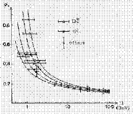
Figure 5.1: $\alpha_{s}$ values deduced from meson masss spectra.

With these results, we can say safely that $\Delta\alpha_{s}\stackrel{{\scriptstyle<}}{{=}}0.001$ at $Q=500{\rm{GeV}}$ so that all kinds of QCD calculations can be carried out within 1% level at this energy. On the other hand, $\alpha_{s}$ becomes greater than 0.5 in low energy region corresponding to light quark hadrons, where perturbative calculations break down. The smooth transition from perturbative region into non-perturbative one cannot be clearly cut off at some point, and there remain some uncertainties in defining the related factorization scales.

5.4 Non-perturbative Topics

5.4.1 Jet Overlapping

In order to describe the non-perturbative features of hadronization processes, we usually assume two generalities ; one is the local parton-hadron duality and the other is the universality of $\alpha_{s}$ in low energy region. With these assumptions we can construct models for hadronizations resulting in various jet generating algorithms such as HERWIG from cluster model, JETSET or UCLA from string model, PYTHIA, PANDORA, ISAJET, SUSYGEN etc. with appropriate corrections. For these algorithms, one important point is that there exist differences between quark jet and gluon jet. These differences could be critical in analyzing many jet systems resulting from high energy, $e^{+}e^{-}$ linear collider.  Another point to be considered in analyzing many jet systems is jet overlapping. For 2 jet system, there exists no problem since the configuration of 2 jets is linear. For 3 jets, the differences between quark jet and gluon jet turn out to be string effects with slight overlapping effects. However, for 4 jet system, the overlapping probability becomes significant. For example, let’s estimate the probability to overlap by assuming jet shapes of cone structure with subtending solid angle $\frac{\pi}{16}$, which corresponds approximately to a cone with side angle $\frac{\pi}{6}$. For a fixed cone, the total solid angle for another cone to overlap becomes $\frac{9}{16}\pi$. Then the probability for 3 fixed cones to overlap with the remaining one is $\frac{27}{64}$, which is larger than $\frac{1}{3}$. This probability becomes $\frac{9}{16}$ for 5 jet system and increases to $\frac{45}{64}$ for 6 jets. Since $t\bar{t}$ processes in linear collider correspond to 6 jet system, it becomes problematic to analyze $t\bar{t}$ by just counting particle trajectories. The situation becomes worse if we want to get some information about particle polarizations. Moreover, the $t\bar{t}H$ processes result in 8 jets for which the overlap probability becomes $\frac{63}{64}$. In our simple estimation, jets cannot be separately observed in 8 jet system so that it is meaningless to follow particle trajectories to define jets.

Since we have to be prepared to account for many jets such as 10 or 20 jets in high energy linear collider, we need to construct new theoretical models which can be used to analyze jet overlapping. One possibility is the momentum space flux-tube model which will be explained in the following sections. We can classify flux-tubes and construct topological spaces and then it is possible to define probability amplitude to have quark pairs which can be used to predict particle multiplicities in jets. In this way, we can account for string effects in 3-jets by considering appropriate differences between quark and gluon jets.

5.4.2 Flux-Tube Model

The flux-tube model was originally considered in order to account for the mass spectra of hadrons and their strong decay processes which are related to quark pair creations. At first, the creations of quark pairs were assumed arbitrarily with appropriate operators resulting in models such as the ${}^{3}P_{0}$ or the ${}^{3}S_{1}$ model. However, it was thought later that the quark pair creations were controlled by gluonic degrees of freedom. It is well known that the gluonic degrees of freedom in bound state problems are not so simple as to be described by perturbative calculations only. The non-perturbative feature of gluonic interactions is one of the motives for consideration of the simple flux-tube formalism.

The description of gluonic flux-tube was firstly attempted by a string picture. In quark pair creation model, the created quark pair breaks a flux-tube with equal probability amplitude anywhere along the string and in any state of string oscillation. The amplitude to decay into a particular final state is assumed to depend on the overlap of original wave functions of quarks and string with the final two state wave functions separated by the pair creation. For ground state strings connecting quark and antiquark in mesons, the amplitude $\gamma(\xi\vec{r},\vec{\omega})$ to break at point $\frac{\vec{r}}{2}+\vec{\omega}$ was first assumed to be[28]

$$\gamma(\xi\vec{r},\vec{\omega})=\omega_{0}e^{-\frac{b}{2}\omega^{2}_{min}}$$ (5.19)

where $\gamma_{0}$ and $b$ are parameters and

$$\frac{\vec{r}}{2}+\vec{\omega}=\vec{r}_{\bar{q}}+\xi\vec{r}+\vec{\omega}_{min}$$ (5.20)

with $\vec{r}=\vec{r}_{q}-\vec{r}_{\bar{q}}$ being the difference between the quark and the antiquark position vectors. $\vec{\omega}_{min}$ is the vector with the shortest distance between any point on the vector $\vec{r}$ and the pair creation point, and $\xi$ measures the ratio of the distances from the original antiquark and quark positions to the projection point of the created quark pair along the vector $\vec{r}$ . The shape of equi-$\gamma$ surface looks like a cigar which is appropriate to describe a flux-tube of constant width with end caps.

For general shapes, we can introduce a $\xi$-dependent factor $f(\xi)$ into the exponent of $\gamma$ such that

$$\gamma_{f}=\gamma_{0}e^{-\frac{1}{2}f(\xi)b\omega^{2}_{min}}.$$ (5.21)

Although it has been found that physical results are nearly independent of $f(\xi)$ for $\frac{1}{3}<f<3$, the arbitrariness of $f(\xi)$ raises the problem of theoretical basis for the derivation of flux-tube overlap function $\gamma$. In fact, the form in Eq.(4-2-3) was derived by using harmonic oscillator wave functions for discrete string components. The form was even changed into the spherical one[29]

$$\gamma(\vec{r},\vec{\omega})=\gamma_{0}e^{-\frac{b}{2}\omega^{2}}$$ (5.22)

which is convenient for calculating physical amplitudes expanded in the harmonic oscillator wave function basis. The changes in the form of $\gamma$ indicate the fact that no firm theoretical grounds exist for treating gluonic flux-tubes.

5.4.3 Construction of Topological Spaces

In order to deduce flux-tube overlap functions systematically from a well-defined set of assumptions, we need to devise a framework for the description of gluonic flux-tubes. Since the QCD bound-state problem with strong couplings has not been solved as yet, we have to assume the existence of gluonic flux-tubes and their interactions. The most fundamental interactions between flux-tubes are their joining and breaking processes, and these two processes with the existence assumption make it possible to devise a topological approach to the description of flux-tubes[30]. To construct topological spaces, we need to classify the flux-tubes, and it can be done by counting the number of boundary points which are occupied by a quark or an antiquark behaving as a source or a sink. The classified sets of flux-tubes can be represented as $F_{a,\bar{b}}$ which means the flux-tube set with a quarks and b anti-quarks sitting at boundary points. For convenience, we omit the number if it becomes zero except for $F_{0}$ which represents the set with no boundary point, that is, the flux-tube set corresponding to glueballs.

We can construct topological spaces on the classified flux-tube sets with the following assumptions :

(1) Open sets are stable flux-tubes.
(2) The union of stable flux-tubes becomes a stable flux-tube.
(3) The intersection between a connected stable flux-tube and disconnected stable flux-tubes is the reverse operation of the union.

There are two possible senarios distinguished by the condition whether the set $F_{0}$ is included or not. If $F_{0}$ is included, the loop structure can be added to any flux-tube by the union operation. Then, the loop can be broken by the intersection operation with one quark-antiquark pair created as new boundaries. When we exclude four-junction structures in flux-tubes, inclusion of $F_{0}$ corresponds to the creation of two three-junctions. In this case, we can conclude that all kinds of flux-tube sets are interrelated through the union and intersection operations if the condition of baryon number conservation is satisfied. Therefore, topological spaces have to be formed with all these sets under the restriction of baryon number conservation.

When $F_{0}$ is not included in the construction of topological spaces, we can exclude three-junction creations by assuming the existence of only non-excited flux-tubes. For this case, we can construct various topological spaces such as meson, baryon-meson, antibaryon-meson, baryon-meson-baryon systems, and so on. Let’s consider first the meson system $F_{1,\bar{1}}$. A meson can decay into several mesons by repeated pair creations and if we represent n meson states by $F^{n}_{1,\bar{1}}$, the simplest non-trivial topological space is given by

$$T_{0}~{}=~{}\{\phi,~{}F_{1,\bar{1}},~{}F^{2}_{1,\bar{1}},~{}\cdots~{},~{}F^{n}_{1,\bar{1}},~{}\cdots~{}\}$$ (5.23)

Since $F_{1,\bar{1}}$ represents the set of all possible flux-tubes with two boundary points, there is no confusion in writing

$$F^{2}_{1,\bar{1}}~{}=~{}F_{1,\bar{1}}$$ (5.24)

Then $T_{0}$ becomes

$$T_{0}=\{\phi,F_{1,{\bar{1}}}\}$$ (5.25)

If we accept that $F_{1,\bar{1}}$ can be multiplied at any time without violation of baryon number conservation, the topological space for baryon-meson system can be written as

$$T_{1,0}~{}\equiv~{}T_{1}~{}=~{}\{\phi,~{}F_{3},~{}F_{3}F_{1,\bar{1}}\}~{}=~{}\{\phi,~{}F_{3}\}$$ (5.26)

and in general, we get

$$T_{i,\bar{j}}=\{\phi,~{}F^{i}_{3}F^{j}_{\bar{3}},~{}F^{i-1}_{3}F^{j-1}_{\bar{3}}F_{2,\bar{2}},~{}\cdots~{}\}$$ (5.27)

5.4.4 Connection Amplitude

For the defined topological spaces, we can consider the connection amplitude A for a quark to be connected to another quark or anti-quark through the given flux-tube open set. In general, we can assume the existence of a measure $M$ of the connection amplitude A satisfying the conditions that

(1) $M(A)$ decreases as A increases,
(2) $M(A_{1})+M(A_{2})=M(A_{1}A_{2})$ when $A_{1}$ and $A_{2}$ are independent.

The multiplication of two independent amplitudes $A_{1}$ and $A_{2}$ is induced by the union operation. The above two conditions for the measure of the connection amplitude lead to the solution

$$M(A)=-k\ln\frac{A}{A_{0}}$$ (5.28)

where $A_{0}$ is a normalization constant and $k$ is an appropriate parameter. In order to get coordinate dependences, we consider the measure $M$ as a metric through a flux-tube between two points occupied usually by quark or antiquark. If we consider the simplest flux-tube type $F_{1,\bar{1}}$ the metric can be thought of as functions of $|\vec{x}-\vec{y}|$ with $\vec{x}$ and $\vec{y}$ being the positions of the two boundary points. In general, the distance function $|\vec{x}-\vec{y}|^{\nu}$ can be made metric if it satisfies the triangle inequality

$$|\vec{x}-\vec{z}|^{\nu}+|\vec{z}-\vec{y}|^{\nu}\stackrel{{\scriptstyle>}}{{=}}|\vec{x}-\vec{y}|^{\nu}$$ (5.29)

The set of points $\vec{z}$ not satisfying this triangle inequality can be taken as forming the inner part of the flux-tube where it is impossible to define a metric from boundary points with given $\nu$. With this metric condition, we can figure out the shape of flux-tube, and we can take $|\vec{x}-\vec{y}|^{\nu}$ as an appropriate measure to deduce a concrete form for the connection amplitude A. The lower limit of $\nu$ can be fixed to be 1 because there exists no point $\vec{z}$ satisfying the triangle inequality with $\nu<1$ . In order to account for various possibilities, we need to sum over contributions from different $\nu$’s. For a small increment $d\nu$, the product of the two probability amplitudes for $|\vec{x}-\vec{y}|^{\nu}$ and $|\vec{x}-\vec{y}|^{\nu+d\nu}$ to satisfy the metric conditions can be accepted as the probability amplitude for the increased region to be added to the inner connected region which is out of the metric condition. Then the full connection amplitude becomes

$$A=A_{0}exp\{-\frac{1}{k}\int_{1}^{\alpha}F(\nu)r^{\nu}d\nu\}$$ (5.30)

where all possibilities from the line shape with $\nu=1$ to the arbitrary shape with $\nu=\alpha$ have been included. The weight factor $F(\nu)$ has been introduced in order to account for possible different contributions from different $\nu$’s. When we consider the case of $\alpha=2$, which corresponds to a spherical shape flux-tube, and the case of equal weight $F(\nu)=1$, we get

$$A=A_{0}exp\{-\frac{1}{k}\frac{r^{2}-r}{\ln r}\}$$ (5.31)

Slight changes can be made if we replace A into $r^{\beta}A$, for which the conditions on $M$ still hold with $\beta>0$. Then general $A$ becomes

$$A=\frac{A_{0}}{r^{\beta}}exp\{-\frac{1}{k}\frac{r^{2}-r}{\ln r}\}$$ (5.32)

5.4.5 Gluonic Structures in Hadrons

In order to describe the non-perturbative gluonic structures in hadrons by using flux-tube model, it is necessary to deduce the relationships between the connection amplitude and the long range gluonic distributions. The gluonic contents of hadrons can be probed by estimating the probability amplitudes for quark pair creations because the quark pairs are created by the gluons inside hadrons. If we assume that the probabilities for quark pair creations are proportional to the gluon densities, the gluonic structures of hadrons can be deduced from the flux-tube overlap functions defined by the connection amplitudes. The probability amplitude to have a quark pair at a given position is taken to be equal to the overlap of connection amplitudes calculated for the initial and the final boundary points. The overlap function $\gamma$ can be written as

$$\gamma=A_{i}A_{f}$$ (5.33)

where $A_{i}$ and $A_{f}$ represent the connection amplitudes before and after quark pair creation.

Although the gluonic densities are closely related to physically observable quantities, it is impossible to observe directly the gluonic densities because gluons are confined. During the formation process of final hadrons, quark pairs are created by confined gluons. The confined structures of gluons can be probed only through the created quark pairs, and the probability amplitude to have a quark pair at a specified position is proportional to the overlap function $\gamma$ that can be used to describe gluonic behaviors. We can calculate the overlap function $\gamma$ for various configurations of boundary points.

As the first example, let’s consider the case of a proton accelerated in the positive direction of z-axis. We can assume that electric fields are applied along positive z direction during the acceleration. Then the three boundary quarks will be oriented in such a way that the two positively charged up quarks go ahead pulling the other negatively charged down quark. If the flux-tubes connecting the three boundary quarks do not break, the distance between the up quarks and the down quark will be contracted along the direction of z-axis. The relative positions of three boundary quarks will change according to the Lorentz boosts, and the corresponding gluonic structures will change. If we take different connection amplitudes with different values of $\beta$, the gluonic structures turn out to be deformed from one to another[31]. These structures can be Fourier transformed resulting in gluon distribution functions in momentum space.

In the case of a neutron, the three boundary points are occupied by one up quark and two down quarks. Since the total charge of these three quarks is zero, a neutron cannot be accelerated as for a proton. However, the three quarks can be aligned in an electric field, and if we fix the three boundary points we can calculate the flux-tube overlap functions. We can easily check that the shapes of gluon distribution functions for a proton and for a neutron are different even if we change the velocity of the neutron.

For quarkonium mesons, the situation changes into one with only two boundary points. For example, if we consider the case of $\pi^{+}$ accelerated along z direction, the gluon densities along z direction turn out to be symmetric about the axis through the center point between the u quark and the $\bar{d}$ quark. All the other quarkonium mesons have the similar form.

5.4.6 Momentum Space Formulation

The necessity to transform coordinate space distributions into those in momentum space originates from the nature of scattering processes. In particle scattering processes, the initial and the final states are defined by the momenta of each particle and the final data can be obtained by analyzing particle trajectories. Because the quarks cannot exist alone, hadronization processes are essential to form particles that can generate such trajectories. These hadronization processes cannot be described by perturbative QCD, and we need to construct models to account for non-perturbative features of QCD. In our flux-tube model, we can account for these non-perturbative features which are related to quark pair creations leading to final jets observed in high energies. Since the created quark pairs have to be specified in momentum space for scattering states, we need to formulate our model in momentum space.

Because the connection amplitudes have been defined between two boundary points, it is possible to consider the same amplitudes in momentum space. The connection amplitude for two boundary points with momenta $\vec{p_{1}}$ and $\vec{p_{2}}$ can be written down as

$$A=A_{0}exp\{-\frac{1}{\tau}\int_{1}^{\alpha}G(\nu)|\vec{p_{1}}-\vec{p_{2}}|^{\nu}d\nu\}$$ (5.34)

where $G(\nu)$ and $\alpha$ are an appropriate weight factor and the boundary value of $\nu$ respectively. In case of $G(\nu)=1$ and $\alpha=2$, we get

$$A(p)=A_{0}exp\{-\frac{1}{\tau}\frac{p^{2}-p}{\ln p}\}$$ (5.35)

with $p=|\vec{p_{1}}-\vec{p_{2}}|$. We can apply this amplitude to describe fragmentation processes resulting in jets.

As an example, we choose the 3-jet events formed from fragmentation processes of ${Z^{0}}^{\prime}$s produced by $e^{+}e^{-}$ collisions. For $Z^{0}$ fragmentations, no initial state uncertainties exist, and the final quark jets and antiquark jets can be identified by lepton-tagging methods. For non-trivial 3-jet events, the other gluon jet can be identified clearly and we can compare different properties between quark jet and gluon jet. The gluonic effects appear as the probability amplitudes for creation of quark pairs which generate many hadrons resulting in jets. For the above $A(p)$, the probability amplitude for a created quark pair to be connected in momentum to the quark and the gluon boundaries is proportional to

$$C_{1}=A^{3}_{0}exp\{-\frac{1}{\tau}(\frac{a^{2}-a}{\ln a}+\frac{b^{2}-b}{\ln b}+\frac{c^{2}-c}{\ln c})\}$$ (5.36)

where $a$ and $b$ are the distances in momentum space from the created quark pair to gluon and quark boundaries, and $c$ is the distance between gluon and antiquark boundaries. The other amplitude $C_{2}$ for the created quark pair to be connected to the antiquark and the gluon boundaries has the same form with the interchanged roles of quark and antiquark boundaries. The probability to get particles in a given direction is

$$P=\int_{0}^{h}|C_{1}+C_{2}|^{2}dR$$ (5.37)

where $h$ is determined by phase space configurations. The shape of momentum phase space can be determined by using parton model assumptions. Longitudinal components are taken to be proportional to the total parton energy which becomes generally the total jet energy. On the other hand, transverse components are assumed to be small resulting from uncertainties in momentum specifications. With appropriate choice of phase space, we can predict the particle multiplicities for jet configurations[32]. For 6 data samples from the OPAL group, we have fixed parameters to the first data and then predicted the other 5 samples quite well.

5.5 Summary

Quantum chromodynamics is taken to be the right theory of strong interaction, which is responsible for the formation of hadrons. Since the final states of high energy linear collider will be mostly composed of hadrons, it is important to check the hadronization processes with the viewpoints based on QCD.

The initial particle creation processes can be described by perturbative gauge theories, whereas there exists a transition point from perturbative viewpoints to non-perturbative model constructions. Perturbative QCD calculations are carried out by expanding with respect to $\alpha_{s}$, and it is expected that these expansions can be done within 1% level in the energy range of $500{\rm{GeV}}$. Higher order calculations can be checked with some corrections such as exponentiation or resummation included. However, there exists uncertainty in choosing the transition point from perturbative formalism to non-perturbative one, and we need to study more on this subject. For the non-perturbative hadronization processes, we have to construct models resulting in jet generating algorithms. Although there exist many models, we need more systematic formalism which can be used to explain many jet system such as 10 or 20 jets with overlapped configurations. One possibility is the momentum space flux-tube model which can be applied to explain particle multiplicities, string effects, angular ordering, and so on. However, we have to study more on topics such as color rearrangement, baryon production, and spin polarization.

Chapter 6 Precision Electro-Weak Physics

6.1 Introduction

Total cross sections of standard model processes below 1 TeV are shown in Fig. 6.1. As seen in the figure, productions of multiple gauge bosons are characteristic feature of experiments at JLC. Precise measurements of their properties, such as masses and couplings, allow us to test models at higher order and serve as tools to probe physics at high energy scale. A clean environment, polarized beams, variable collision energies and high luminosities at JLC are essential ingredients for precise measurements. When operated at the $Z$ pole and just above the $W$ pair threshold, Giga $Z$ and Mega $W$ samples can be accumulated. These statistics are two orders of magnitude more than LEP-I/II. At 500 GeV and above, gauge cancellation among diagrams of the $e^{+}e^{-}\rightarrow W^{+}W^{-}$ process becomes severer, which allows us a direct measurement of triple-gauge-boson couplings at a precession required to probe loop effects. At higher energies, processes which involve $t$-channel diagrams increase cross sections with energy, from which $WW$ scattering processes could be measured. In general, models without elementary Higgs bosons predict strong interaction among longitudinal polarized $W$ bosons. Such effects would be observed through the final-state interaction of $W$’s in the $e^{+}e^{-}\rightarrow W^{+}W^{-}$ process or resonance production in processes such as $e^{+}e^{-}\rightarrow\nu\bar{\nu}W^{+}W^{-}$.

In the following subsections, we discuss topics on measurements of the $W$ boson mass and triple-gauge-boson couplings.

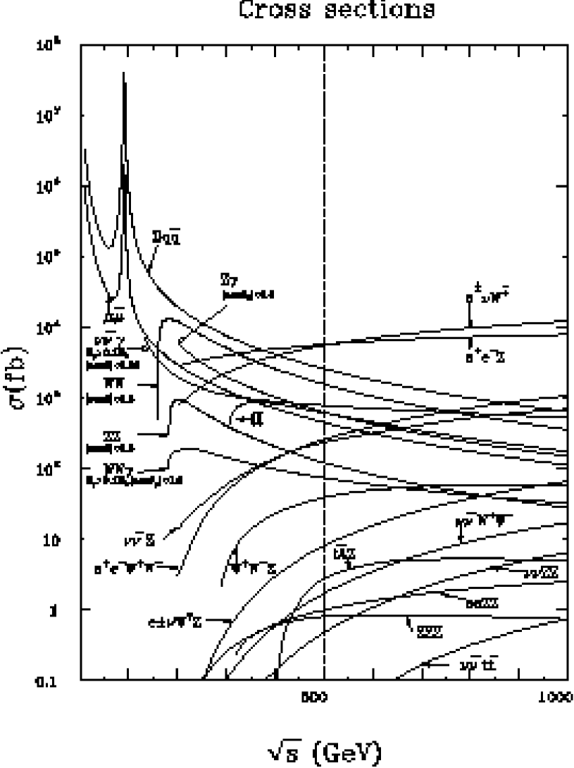
Figure 6.1: Cross sections of the standard model processes at energies below 1 TeV.

6.2 $W$ Boson Mass Determination

The masses of $W$, $t$, and Higgs are related through loop corrections. Their relations are shown in Fig. 6.2. As seen from the figure, the loop effects of the masses of $W$ and $t$ to that of Higgs are quite different in size: if we require the same size, precisions of the $t$ and $W$ masses should satisfy $\sigma_{m_{W}}\sim 0.7\times 10^{-2}\sigma_{m_{t}}$. At JLC, $\sigma_{m_{t}}\sim 100$ MeV is expected for 100 fb^-1, which corresponds to $0.7$MeV for $\sigma_{m_{W}}$. Fig. 6.3, on the other hand, shows 1-$\sigma$ contours in the plane of $m_{t}$-$m_{H}$ for several values of precision for the top quark mass measurement. From this figure, the importance of precise mass determination of the top quark is evident. Since the expected precision of the top quark mass is less than 0.15 GeV, the error on the estimated Higgs mass is dominated by the error of the $W$ mass measurement.

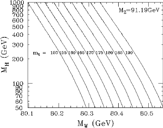
Figure 6.2: The mass of the standard model Higgs boson as a function of the $W$ mass for different top quark masses.

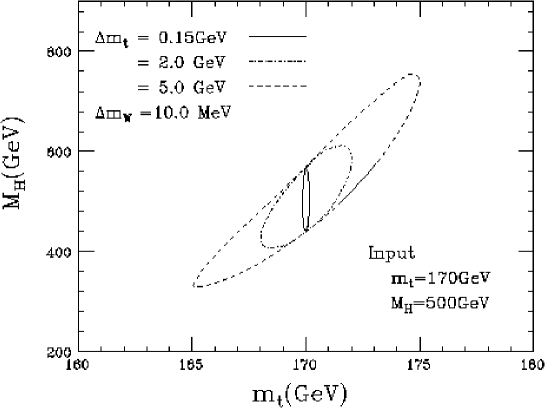
Figure 6.3: 1-$\sigma$ contours in the plane of $m_{t}$-$M_{H}$ for three values of top quark mass error. We used $m_{t}=170$GeV and $M_{H}=500$GeV here.

The current world average for $m_{W}$ is $80.448\pm 0.034$ GeV, which is the average of the LEP2 average of 40 MeV precision and the $p\bar{p}$ average of 62 MeV precision. The $p\bar{p}$ error is expected to be reduced to 30 MeV by Tevatron Run-II and to 15 MeV at LHC. However, the error is still larger than that required by the expected top quark mass error as far as the contribution to the loop effect is concerned. Further improvement of the $m_{W}$ measurement is desirable. If no Higgs boson is discovered at any colliders including the JLC, the precise $m_{W}$ measurement is of vital importance, since the loop effect would be the only way to estimate the Higgs mass. In Fig. 6.4, we show the error in the Higgs mass estimation from the quantum effect as a function of the Higgs mass. If the Higgs boson is there in the JLC energy region , its mass will be measured with a precision similar to the mass of the top quark, as described in the Higgs chapter. The precise determinations of the $W$, $t$, and Higgs masses will enable us to test the standard model at the loop level, thereby allowing us to probe new physics in the loop effect.

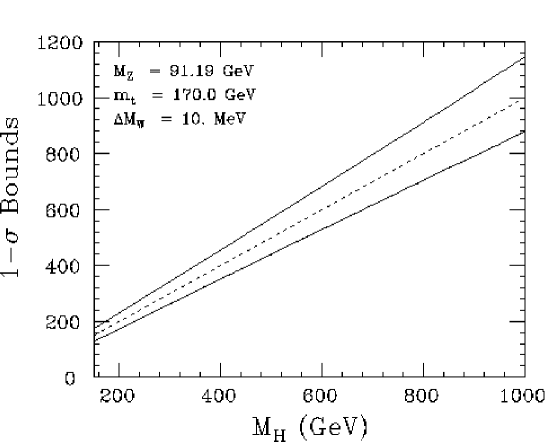
Figure 6.4: 1$\sigma$ bounds of the mass of Higgs as a function of the mass of Higgs, the precision of $W$ mass is 10 MeV.

At JLC the $W$ mass could be measured at $\sqrt{s}=500$ GeV, using the process $e^{+}e^{-}\rightarrow e\nu W$, since it has a large cross section and that there is no ambiguity in selecting particles from the $W$ decay. If we require $|\cos\theta|<0.8$ to select events well contained in the detector acceptance, about 80k events are expected to be observed for 100fb^-1[1]. On the other hand, 40k events of $e^{+}e^{-}\rightarrow\gamma Z$ process can be observed under the same condition. This process can be used for detector calibration. The invariant mass resolution for the Higgs mass of 100 GeV is expected to be less than 4 GeV. If similar resolution can be achieved for $W$’s, we can expect the statistical error of the $W$ mass to be about 20MeV. If the integrated luminosity is 400 fb^-1, which is less than two years of running with JLC-Y parameters, the statistical error of the $W$ mass becomes about 10 MeV. In this measurement, there is no systematic error due to ambiguity in jet clustering or color recombination. If the statistics of the $e^{+}e^{-}\rightarrow\gamma Z$ process is not sufficient for calibration, we might run at the $Z$ pole for higher statistics. We need, however, a serious study to find out possible source of detector systematics.

6.3 Triple and Quartic Gauge Boson Couplings

In the standard model, electroweak gauge bosons are introduced to preserve the local $SU(2)_{L}\times U(1)_{Y}$ symmetry. As a result, there is a universality among the couplings of fermions to the gauge boson, the three gauge bosons, and the four gauge bosons. This universality forms the basis of the success of the standard model ( see Ref.[9] for example ). So far the fermion-gauge-boson couplings were tested precisely at various colliders, however the direct measurement of the self couplings of the gauge bosons is not precise enough to test the standard model at loop level.

In order to formulate the test of the self couplings of the gauge bosons, we usually introduce a Lagrangian containing non-standard-model interactions, assuming some symmetry for them. The most general Lagrangian assuming the electro-magnetic gauge invariance, the Lorentz symmetry, and $C$ and $P$ conservation is given by[10]

$${{\cal L}_{WWV}}/g_{WWV} = ig^{V}_{1}(W_{\mu\nu}^{\dagger}W^{\mu}V^{\nu}-W_{\mu}^{\dagger}V_{\nu}W^{\mu\nu})+i\kappa_{V}W^{\dagger}_{\mu}W_{\nu}V^{\mu\nu}$$ (6.1)

$$+ {i\lambda_{V}\over m^{2}_{W}}W^{\dagger}_{\lambda\mu}W^{\mu}_{\nu}V^{\nu\lambda},$$

where $V\equiv Z$ or $\gamma$ and $W_{\mu\nu}\equiv\partial_{\mu}W_{\nu}-\partial_{\nu}W_{\mu}$, $V_{\mu\nu}\equiv\partial_{\mu}V_{\nu}-\partial_{\nu}V_{\mu}$, $g_{WW\gamma}=-e$, and $g_{WWZ}=-e\cot\theta_{W}$. In the standard model, $g_{1}^{V}=\kappa_{V}=1$ and $\lambda_{V}=0$. The static properties of the $W$, the magnetic dipole moment ($\mu_{W}$) and the electric quadrupole moment ($Q_{W}$), are related to these couplings as

$$\mu_{W} = \frac{e}{2M_{W}}(1+\kappa_{\gamma}+\lambda_{\gamma}),$$ (6.2)

$$Q_{W} = \frac{e}{M^{2}_{W}}(\lambda_{\gamma}-\kappa_{\gamma}).$$ (6.3)

Since $g_{1}^{\gamma}=1$ by the electro-magnetic gauge invariance, five anomalous couplings are involved in Eq. (6.1): $\Delta g_{1}^{Z}\equiv g_{1}^{Z}-1$, $\Delta\kappa_{\gamma}\equiv\kappa_{\gamma}-1$, $\Delta\kappa_{Z}\equiv\kappa_{Z}-1$, $\lambda_{\gamma}$, and $\lambda_{Z}$. If we require the global $SU(2)_{L}$ symmetry for Lagrangian (6.1), we are left with only one non-zero coupling: $\lambda\equiv\lambda_{\gamma}=\lambda_{Z}$. Since the $\lambda$ term has an energy dimension of 6, the requirement of the renormalizability leads us to the standard model Lagrangian. If we require an intrinsic $SU(2)_{L}$ symmetry, we are left with four independent couplings with the relation,

$$1+\Delta g_{1}^{Z}=-\tan^{2}\theta_{W}\frac{\Delta\kappa_{\gamma}}{\Delta\kappa_{Z}}.$$ (6.4)

The number of independent couplings becomes two if, in addition, we allow only dimension-4 couplings. If we further require the most divergent quartic one-loop contribution to the $\rho$ parameter be absent, we will get an additional constraint,

$$\Delta g_{1}^{Z}\cos^{2}\theta_{W}=\Delta\kappa_{\gamma},$$ (6.5)

which will lead us to only one coupling of dimension 4.

Lagrangian of Eq. (6.1) is adequate for the study of anomalous triple-gauge-boson couplings at tree level, but it is not adequate for the study of loop effects and the process involving both triple- and quartic-gauge-boson couplings because it does preserve local $SU(2)_{L}\times U(1)_{Y}$ gauge invariance[11]. One approach to overcome this problem is to use the most general $SU(2)_{L}\times U(1)_{Y}$ gauge invariant effective Lagrangian of dimension 6, assuming a Higgs boson, in the studies of the possible low energy effects of new physics at high energy. Another approach is to use the gauged chiral Lagrangian without introducing the Higgs field.

In the locally-$SU(2)_{L}\times U(1)_{Y}$-gauge-invariant dimension-6 effective Lagrangian, the terms involving self-couplings of gauge bosons at tree level can be written in the form[12]:

$${\cal L}=\frac{f_{WWW}}{\Lambda^{2}}O_{WWW}+\frac{f_{W}}{\Lambda^{2}}O_{W}+\frac{f_{B}}{\Lambda^{2}}O_{B},$$ (6.6)

where

$$O_{WWW} = Tr\left[\hat{W}_{\mu\nu}\hat{W}^{\nu\rho}\hat{W}_{\rho}^{\mu}\right],$$

$$O_{W} = (D_{\mu}\Phi)^{\dagger}\hat{W}^{\mu\nu}(D_{\nu}\Phi),$$ (6.7)

$$O_{B} = (D_{\mu}\Phi)^{\dagger}\hat{B}^{\mu\nu}(D_{\nu}\Phi).$$

$\Phi$ is a Higgs doublet field, $D_{\mu}$ is the covariant derivative as given by

$$D_{\mu}\equiv\partial_{\mu}+\frac{i}{2}g^{\prime}B_{\mu}+ig\frac{\sigma^{a}}{2}W_{\mu}^{a},$$

and the hatted field operators are defined as $\left[D_{\mu},D_{\nu}\right]=\hat{W}_{\mu\nu}+\hat{B}_{\mu\nu}$. Since the operators in Lagrangian (6.6) have dimension 6, it is unrenormalizable and the scale $\Lambda$ can be identified as the cut-off energy. $f_{WWW}$, $f_{W}$, and $f_{B}$ are the anomalous couplings of corresponding terms.

In terms of these couplings, the couplings in Lagrangian (6.1) are expressed as

$$\Delta g_{1}^{Z} = f_{W}\frac{m^{2}_{Z}}{2\Lambda^{2}},$$ (6.8)

$$\Delta\kappa_{Z} = \left[f_{W}-\sin^{2}\theta_{W}(f_{B}+f_{W})\right]\frac{m^{2}_{Z}}{2\Lambda^{2}},$$ (6.9)

$$\Delta\kappa_{\gamma} = \cos^{2}\theta_{W}(f_{B}+f_{W})\frac{m^{2}_{Z}}{2\Lambda^{2}},$$ (6.10)

$$\lambda_{\gamma} = \lambda_{Z}=\frac{3m^{2}_{W}g^{2}}{2\Lambda^{2}}f_{WWW}.$$ (6.11)

Because of Eqs. (6.8) - (6.11), only three of the five couplings in Eq. (6.1) are independent.

Here the above constraints are consequences of the electroweak gauge invariance and the restriction to the dimension-6 operators[12]. Since Lagrangian (6.1) involves only the terms relevant to the triple-gauge-boson couplings, we shall use Lagrangian (6.6) for the study of self-couplings in the JLC energy region, where the quartic-gauge-boson couplings are equally important at tree level.

In the following discussion, we use $\Delta\kappa_{\gamma}$, $\Delta\kappa_{Z}$, and $\lambda$ to parametrize the three free parameters of Lagrangian (6.6) unless otherwise stated, where $\lambda\equiv\lambda_{\gamma}=\lambda_{Z}$ which is proportional to $f_{WWW}$ as Eq. (6.11), and

$$\Delta g_{1}^{Z}=\Delta\kappa_{Z}+\tan^{2}\theta_{W}\Delta\kappa_{\gamma},$$ (6.12)

due to constraints (6.8) - (6.10). In terms of $\Delta\kappa_{\gamma}$ and $\Delta\kappa_{Z}$, $f_{W}$ and $f_{B}$ are expressed as

$$f_{W} = \frac{2\Lambda^{2}}{m^{2}_{Z}}(\Delta\kappa_{Z}+\tan^{2}\theta_{W}\Delta\kappa_{\gamma}),$$ (6.13)

$$f_{B} = \frac{2\Lambda^{2}}{m^{2}_{Z}}(\Delta\kappa_{\gamma}-\Delta\kappa_{Z}).$$ (6.14)

It should be noted that in this convention[12], a given set of the anomalous couplings ($\Delta\kappa_{\gamma}$, $\Delta\kappa_{Z}$, $\lambda$) should necessarily contain the $\Delta g_{1}^{Z}$ term (6.12) as well as the quartic couplings in (6.6).

The standard model processes at JLC which involve the triple- and quartic-gauge-boson couplings at tree level are summarized in Table 6.1. First and second columns show vertices and couplings. The vertices $WW\gamma Z$, $WWZZ$, and $WWWW$ involve $\Delta\kappa_{\gamma}$ and $\Delta\kappa_{Z}$ couplings. But, since they are proportional to $\Delta\kappa_{\gamma}-\Delta\kappa_{Z}$, they are indicated by $f_{W}$ ( $\equiv\frac{2\Lambda^{2}}{m^{2}_{Z}}(\Delta\kappa_{\gamma}-\Delta\kappa_{Z}$)). $\bigcirc$’s in the rest of the columns indicate processes which involve the relevant vertices. The processes marked by $\bigtriangleup$ involve corresponding vertices, but the sensitivities are limited. The last row of the table shows the total cross sections at $\sqrt{s}=500$ GeV, where $E_{\gamma}>25$ GeV and $|\cos\theta_{\gamma}|<0.85$ are required for the processes $\nu\bar{\nu}\gamma$ and $WW\gamma$, and $|\cos\theta|<0.9$ is assumed for $\gamma\gamma\rightarrow W^{+}W^{-}$[13].

Table 6.1: Processes and couplings at tree level.

$e^{+}e^{-}\rightarrow$ $\gamma\gamma\rightarrow$ Vertex Couplings $WW$ $e\nu W$ $\nu\bar{\nu}\gamma$ $\nu\bar{\nu}Z$ $WWZ$ $WW\gamma$ $eeWW$ $WW$ $WW\gamma$ $\lambda,\Delta\kappa_{\gamma}$ $\bigcirc$ $\bigcirc$ $\bigcirc$ $\bigcirc$ $\bigcirc$ $\bigcirc$ $\bigcirc$ $WWZ$ $\lambda,\Delta\kappa_{Z}$ $\bigcirc$ $\bigtriangleup$ $\bigcirc$ $\bigcirc$ $\bigcirc$ $\bigcirc$ $WW\gamma\gamma$ $\lambda$ $\bigcirc$ $\bigcirc$ $\bigcirc$ $WW\gamma Z$ $\lambda,f_{W}$ $\bigcirc$ $\bigcirc$ $\bigcirc$ $WWZZ$ $\lambda,f_{W}$ $\bigcirc$ $\bigcirc$ $\bigtriangleup$ $WWWW$ $\lambda,f_{W}$ $\bigcirc$ $\sigma$ at $\sqrt{s}=500$ GeV (fb) $8\times 10^{3}$ $6\times 10^{3}$ $10^{3}$ $350$ $60$ $80$ $400$ $50\times 10^{3}$

In the approach using the chiral Lagrangian[2, 3, 4], the physical Higgs field is dropped while the Goldstone fields are included to give masses to the gauge bosons. To this end, the unitary matrix operator, $U(x)$, consisting of the Goldstone fields, $\omega^{a}$, is defined:

$$U(x)\equiv\exp\left(\frac{i\tau^{a}\omega^{a}}{v}\right)$$ (6.15)

Using $U(x)$, the Lagrangian for the kinetic terms of the gauge fields and the Higgs doublet is given by

$${\cal L}_{sm}={v^{2}\over 4}{\rm tr}(D_{\mu}U^{\dagger}D^{\mu}U)-{1\over 2}{\rm tr}({\cal W}_{\mu\nu}{\cal W}^{\mu\nu})-{1\over 2}{\rm tr}({\cal B}_{\mu\nu}{\cal B}^{\mu\nu}).$$ (6.16)

where

$${\cal W}_{\mu} \equiv {\tau^{a}\over 2}W^{a}_{\mu},$$

$${\cal W}_{\mu\nu} \equiv \partial_{\mu}{\cal W}_{\nu}-\partial_{\nu}{\cal W}_{\mu}+ig_{2}\left[{\cal W}_{\mu},{\cal W}_{\nu}\right],$$

$${\cal B}_{\mu} \equiv {\tau^{3}\over 2}B_{\mu},$$

$${\cal B}_{\mu\nu} \equiv \partial_{\mu}{\cal B}_{\nu}-\partial_{\nu}{\cal B}_{\mu},$$

$$D_{\mu}U \equiv \partial_{\mu}U+ig_{2}{\cal W}_{\mu}U-ig_{Y}U{\cal B}_{\mu}.$$ (6.17)

$W^{a}_{\mu}$ and $B_{\mu}$ are $SU(2)_{L}$ and $U(1)$ gauge fields, respectively.

If new physics at some high energy scale affects properties of the gauge boson at low energy, it will produce non-standard terms in the Lagrangian. The general terms of dimension up to 4 is

$${\cal L} = +\beta_{1}{v^{2}\over 4}{\rm tr}({V_{\mu}T}){\rm tr}({V^{\mu}T})+\alpha_{1}g_{2}{\rm tr}\left({\cal W}^{\mu\nu}U{\cal B}_{\mu\nu}U^{\dagger}\right)$$ (6.18)

$$+ i\alpha_{2}g_{Y}{\rm tr}\left(U^{\dagger}\left[V_{\mu},V_{\nu}\right]U{\cal B}^{\mu\nu}\right)+i\alpha_{3}g_{2}{\rm tr}\left(\left[V_{\mu},V_{\nu}\right]{\cal W}^{\mu\nu}\right)$$

$$+ \alpha_{4}{\rm tr}(V_{\mu}V_{\nu}){\rm tr}(V^{\mu}V^{\nu})+\alpha_{5}{\rm tr}(V_{\mu}V^{\mu}){\rm tr}(V_{\nu}V^{\nu})$$

$$+ \alpha_{6}{\rm tr}(V_{\mu}V_{\nu}){\rm tr}(TV^{\mu}){\rm tr}(TV^{\nu})+\alpha_{7}{\rm tr}(V_{\mu}V^{\mu}){\rm tr}(TV_{\nu}){\rm tr}(TV^{\nu})$$

$$+ {1\over 4}\alpha_{8}g_{2}^{2}{\rm tr}(T{\cal W}_{\mu\nu}){\rm tr}(T{\cal W}^{\mu\nu})+{i\over 2}\alpha_{9}g_{2}{\rm tr}(T{\cal W}_{\mu\nu}){\rm tr}(T\left[V^{\mu},V^{\nu}\right])$$

$$+ {1\over 2}\alpha_{10}{\rm tr}(TV_{\mu}){\rm tr}(TV^{\mu}){\rm tr}(TV_{\nu}){\rm tr}(TV^{\nu})+\alpha_{11}g_{2}\epsilon^{\mu\nu\rho\lambda}{\rm tr}(TV_{\mu}){\rm tr}(V_{\nu}{\cal W}_{\rho\lambda}),$$

where $V_{\mu}\equiv D_{\mu}U\cdot U^{\dagger}$, $T\equiv U\tau^{3}U^{\dagger}$, and $\epsilon_{0123}=-\epsilon^{0123}=1$. $\beta_{1}$ is the chiral coupling of energy dimension 2 and $\alpha_{1}\sim\alpha_{11}$ are dimension-4 chiral couplings. Among the 12 couplings in Eq. 6.18, $\beta_{1}$ and $\alpha_{6}\sim\alpha_{10}$ violate custodial symmetry. $\alpha_{11}$ conserves $CP$ but violates $P$ invariance.

The triple- and quartic-self-coupling vertices of the gauge bosons, the chiral couplings involved, and the processes involving these vertices are shown in Table 6.2.

Table 6.2: The chiral couplings involved in the triple- and quartic-gauge-boson vertices. A $\bigcirc$ is shown if the corresponding coupling is involved in the vertices. The processes which are sensitive to the vertices are shown in the right-most column.

vertex	$\alpha_{1}$	$\alpha_{2}$	$\alpha_{3}$	$\alpha_{4}$	$\alpha_{5}$	$\alpha_{6}$	$\alpha_{7}$	$\alpha_{8}$	$\alpha_{9}$	$\alpha_{10}$	$\alpha_{11}$	$\beta_{1}$	processes
$WW\gamma$	$\bigcirc$	$\bigcirc$	$\bigcirc$					$\bigcirc$	$\bigcirc$				$\rightarrow WW$, $e\nu W$
$WWZ$	$\bigcirc$	$\bigcirc$	$\bigcirc$					$\bigcirc$	$\bigcirc$		$\bigcirc$	$\bigcirc$	$\rightarrow WW$, $e\nu W$
$ZZWW$	$\bigcirc$		$\bigcirc$		$\bigcirc$		$\bigcirc$					$\bigcirc$	$\rightarrow WWZ$
$ZWZW$	$\bigcirc$		$\bigcirc$	$\bigcirc$		$\bigcirc$						$\bigcirc$	$\rightarrow WWZ$
$Z\gamma WW$	$\bigcirc$		$\bigcirc$									$\bigcirc$	$\rightarrow WW\gamma$
$ZZZZ$				$\bigcirc$	$\bigcirc$	$\bigcirc$	$\bigcirc$			$\bigcirc$			$\rightarrow ZZZ$

$\alpha_{1}$, $\alpha_{8}$, and $\beta_{1}$ are included in two-point function and expressed in terms of $S$, $T$, and $U$ parameters as follows[2]:

$$\alpha_{1}=-\frac{S}{16\pi},\;\;\alpha_{8}=-\frac{U}{16\pi},\;\;\beta_{1}=\frac{1}{2}\alpha_{em}T$$ (6.19)

Using the PDG values of $S$, $T$, and $U$[18], we get

$$\alpha_{1} = 0.00139\pm 0.0022$$ (6.20)

$$\alpha_{9} = -0.0022\pm 0.0030$$ (6.21)

$$\beta_{1} = -0.003\pm 0.0005$$ (6.22)

If we neglect the terms including $\alpha_{1}$, $\beta_{1}$, and $\alpha_{8}$, the anomalous triple-gauge-boson couplings, $\Delta\kappa_{\gamma}$, $\Delta\kappa_{z}$, and $\Delta g_{1}^{Z}$, can be expressed in terms of $\alpha_{2}$, $\alpha_{3}$, and $\alpha_{9}$ as follows:

$$\Delta\kappa_{\gamma} = {e^{2}\over\sin^{2}\theta_{W}}(\alpha_{2}+\alpha_{3}+\alpha_{9})$$

$$\Delta\kappa_{Z} = {e^{2}\over\cos^{2}\theta_{W}}\alpha_{2}+{e^{2}\over\sin^{2}\theta_{W}}(\alpha_{3}+\alpha_{9})$$ (6.23)

$$\Delta g_{1}^{Z} = {e^{2}\over\sin^{2}\theta_{W}\cos^{2}\theta_{W}}\alpha_{3}.$$

Since the $\alpha_{9}$ coupling violates the custodial $SU(2)$ symmetry, genuine triple-gauge-boson couplings are $\alpha_{2}$ and $\alpha_{3}$, if the custodial symmetry is imposed.

6.4 Sensitivity to the Anomalous Gauge Boson Couplings

The sensitivities to the triple and quartic couplings at JLC were studied in Ref. [1]. Results are summarized in Table. 6.3. In the table, $\sqrt{s}=500$ GeV and the integrated luminosity of 50fb^-1 are assumed. The limits in the plane of $\Delta\kappa_{\gamma}$ and $\lambda$ are shown in Fig. 6.5. In the table and the figure, the couplings other than under study are set to zero to derive the limits.

Among the processes studied, the process $e^{+}e^{-}\rightarrow W^{+}W^{-}$ gives the most stringent bounds. Nevertheless, since the $WW$ process involves all the three couplings, the bounds from the processes $e\nu W$, $\nu\bar{\nu}\gamma$, and $\nu\bar{\nu}Z$ will provide complementary information. Limits obtained from the processes $e^{+}e^{-}\rightarrow e\nu W$, and $e^{+}e^{-}W^{+}W^{-}$ will improve if polarization information of $W$ is used. In the single parameter case, the bounds on $\Delta\kappa_{\gamma}$ and $\Delta\kappa_{Z}$ are less than 1%, and we may have some sensitivity to new physics that gives rise to these effective interactions.

Sensitivities to the chiral couplings, $\alpha_{4}$ and $\alpha_{5}$, through the process, $e^{+}e^{-}\rightarrow W^{+}W^{-}Z$, were studied in Ref.[5]. Assuming the integrated luminosity of 50 fb^-1 at $\sqrt{s}=500$ GeV, sensitivities of about 0.5 at the 95% C.L. are expected. These couplings are sensitive to scalar resonances and higher energy is preferred to get higher sensitivities.

Table 6.3: Summary of sensitivities of various processes to anomalous couplings at the 95 % CL, assuming $\sqrt{s}=500$ GeV and 50 fb^-1 integrated luminosity. In the table, $X_{W}\equiv\cos\Theta_{W}$, $X_{q}\equiv\cos\theta_{q}$, and $X_{l}\equiv\cos\theta_{l}$.

Process		$\Delta\kappa_{\gamma}$	$\Delta\kappa_{Z}$	$\lambda$	method
$e^{+}e^{-}\rightarrow$
	$W^{+}W^{-}$	$-0.0052\sim 0.0057$	$-0.0064\sim 0.0062$	$-0.012\sim 0.021$	$d\sigma/dX_{W}d|X_{q}|dX_{l}$
	$e\nu W$	$-0.021\sim 0.020$	$-$	$-0.039\sim 0.038$	$d\sigma/d|X_{q}|$
	$\nu\bar{\nu}\gamma$	$-0.071\sim 0.075$	$-$	$-0.044\sim 0.079$	$d\sigma/dE_{\gamma}$
	$\nu\bar{\nu}Z$	$-$	$-0.29\sim 0.25$	$-0.46\sim 0.17$	$\sigma_{tot}$
	$W^{+}W^{-}\gamma$	$-0.020\sim 0.016$	$-0.018\sim 0.025$	$-0.025\sim 0.028$	$d\sigma/dE_{\gamma}$
	$W^{+}W^{-}Z$	$-0.053\sim 0.041$	$-0.071\sim 0.15$	$-0.050\sim 0.030$	$\sigma_{total}$
	$e^{+}e^{-}W^{+}W^{-}$	$-0.032\sim 0.039$	$-$	$-0.084\sim 0.12$	$\sigma_{total}$

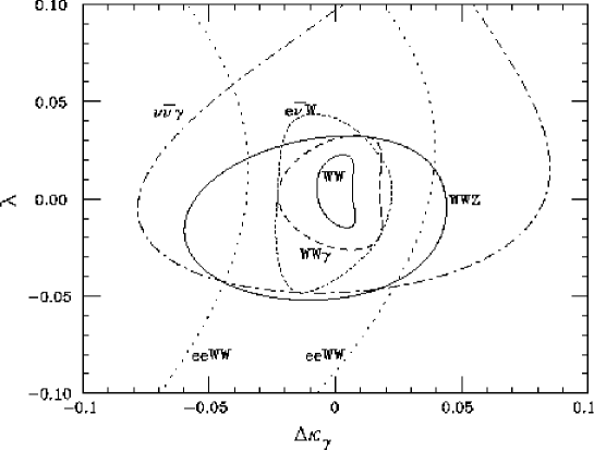
Figure 6.5: Comparison of contours for various processes at the 90% CL in the plane of $\Delta\kappa_{\gamma}$ vs $\lambda$.

6.5 Heavy Higgs and $WW$ Scattering

Even if no light Higgs boson is observed at JLC experiment at the center of mass energy below 500 GeV, its mass could be estimated from the precise measurements of the electroweak interaction. If the expected mass is less than 1 TeV, JLC could increase the energy and the luminosity to cross the threshold. If the Higgs boson is heavy, the major diagram for Higgs boson production is the $W$ fusion process shown in Fig.6.6.

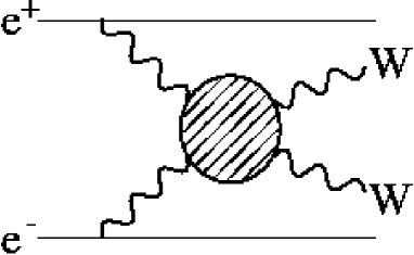
Figure 6.6: A Feynman diagram for the $W$ fusion process.

The background processes to the $W$ fusion process are

$$e^{+}e^{-} \rightarrow W^{+}W^{-}$$ (6.24)

$$\rightarrow \nu_{e}\bar{\nu_{e}}Z^{0}Z^{0}$$ (6.25)

$$\rightarrow e^{\pm}\mathop{\nu_{e}}\limits^{\mbox{\tiny$(-)$}}W^{\mp}Z^{0}$$ (6.26)

$$\rightarrow e^{+}e^{-}Z^{0}Z^{0}$$ (6.27)

$$\rightarrow W^{+}W^{-}.$$ (6.28)

The cross sections of these processes were calculated by GRACE[7]. In these calculations, a care has to be taken so as not to violate the unitarity of the scattering amplitudes, as the couplings of heavy Higgs boson are strong. We thus enlarge the width of the Higgs boson artificially to keep the amplitude below the unitarity limit. This method leads to a conservative estimate of the Heavy Higgs signal.

The Heavy Higgs boson predominantly decays to a $W$ pair, thus a Higgs resonance is expected to be observed as a peak in the $WW$ mass distribution. The invariant mass distributions of $WW$ for several Higgs mass values are shown in Fig.6.7.

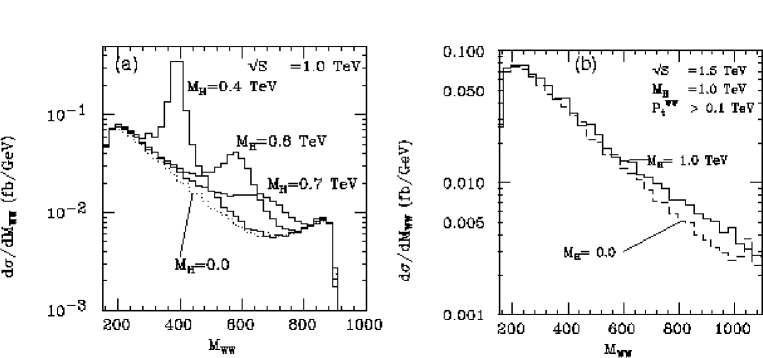
Figure 6.7: (a) invariant mass distributions of $WW$ at $\sqrt{s}$=1 TeV for Higgs masses of 0, 400, 600, and 700 GeV. (b) similar plots at $\sqrt{s}$=1.5 TeV for Higgs masses of 1.0 TeV and 0 TeV.

As seen from the figure, the width of Higgs boson increases with mass and for the Higgs mass of 1 TeV, no clear peak structure in the $WW$ invariant mass distribution can be seen.

We studied the heavy Higgs signal using the Monte Carlo detector simulation[16]. We studied two cases, one at $\sqrt{s}=$ 1 TeV and a Higgs mass of 0.7 TeV, the other at $\sqrt{s}=1.5$ TeV and a Higgs mass of 1.0 TeV. We selected hadronic decays of $W$ as follows. First, we required four jets be observed in the detector and both masses of two jet-pairs be consistent with the $W$ mass. Backgrounds at this stage of selection were 4-jet events from $e^{+}e^{-}\rightarrow e^{+}e^{-}W^{+}W^{-}$ and $e^{+}e^{-}Z^{-}Z^{0}$ processes. These processes were rejected by vetoing energetic $e^{\pm}$. When $e^{\pm}$’s are undetected as they escaped into the uncovered region around the beam pipe, the remaining $W$ pair can not have a large missing $p_{t}$. We could thus eliminate most of the background events by requiring that the $W$ pair system had to have a large missing transverse momentum. The $W$’s from Higgs decays have high longitudinal polarization, while those from other sources do not. The Higgs signal could hence be enhanced if we required jet production angle in the $W$ rest frame be large.

The invariant mass distributions of the $W$ pairs in the selected events for the integrated luminosity of 200fb^-1 are shown in Fig. 6.8.

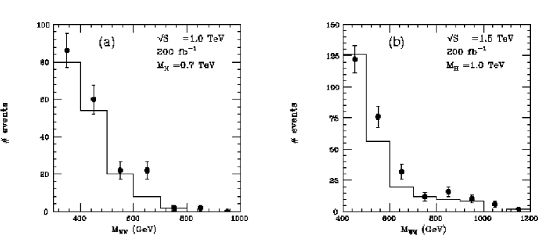
Figure 6.8: The invariant mass distribution of $W$ pairs at (a) $\sqrt{s}=$1.0 TeV and the integrated luminosity of 200fb^-1 and (b) $1.5$ TeV. Histograms are for the Higgs mass of 0 TeV and data points are for 0.7 TeV(a) and 1.0 TeV(b), respectively.

For both of the cases, we could see Higgs effect at statistical significance of 3-sigma[14].

The studies of the $WW$ fusion processes are sensitive to J=0 and J=1 components of the $WW$ scattering amplitude. If new strong interaction is responsible for the $W$ mass generation, it may produce resonances in J=1 channel, which can be probed by a study of the $e^{+}e^{-}\rightarrow W^{+}W^{-}$ process[4]. Since the center of mass energy of the $WW$ system is larger than that of the $WW$ fusion process for a given $\sqrt{s}$, higher sensitivity to the J=1 channel is expected.

A study was performed assuming a vector resonance strongly coupled to the longitudinally polarized $W_{L}W_{L}$[16]. If its mass is low enough, its effect could be observed as anomalous behavior when $W_{L}W_{L}$ is produced in the $e^{+}e^{-}\rightarrow W^{+}W^{-}$ process. For simulation study, we introduce the effect by a form factor, $F(q^{2})$, in the $W_{L}W_{L}$ amplitude. With this form factor, the cross section is expressed as

$$\sigma\propto|\sum_{(ij)\neq(LL)}M_{(ij)}+M^{J\neq 1}_{(LL)}+M^{J=1}_{(LL)}\times F(q^{2})|,$$ (6.29)

where $M^{J=k}_{(i,j)}$ is the scattering amplitude of the $e^{+}e^{-}\rightarrow W^{+}W^{-}$ process and the subscript $(i,j)$ is the polarization of the $W$’s and the superscript $(J=k)$ is the angular momentum of the $W$ pair.

Two types of form factors were investigated: the Breit-Wigner type and those calculated based on the N/D method[15]. The Breit-Wigner-type form factor is expressed as

$$F(q^{2})=-{m_{V}^{2}\over q^{2}-m_{V}^{2}+i\,m_{V}\,\Gamma_{V}\,({q^{2}\over m_{V}^{2}})},$$ (6.30)

where $m_{V}$ and $\Gamma_{V}$ are the mass and the width of the vector resonance, respectively. It turns out that at $\sqrt{s}=500$ GeV, the $\Gamma_{V}$ dependence of the Breit-Wigner form factor is negligible if the mass is greater than 1 TeV and the width is, say, below 400 GeV. We therefore fixed the width at 100 GeV in the analysis. In the case of the N/D method the form factor is expressed as a function of the masses of the scalar resonance ($m_{S}$), the vector resonance($m_{V}$), and the ratio ($r$) of the contribution of the scalar and vector resonances[15]. Since the scalar resonance does not contribute to the $J=1$ channel of the $e^{+}e^{-}\rightarrow W^{+}W^{-}$ process, we fixed $m_{S}=$ 1 TeV.

With the detector simulation, we studied the $e^{+}e^{-}\rightarrow W^{+}W^{-}$ process where one $W$ decays to $e$ or $\mu$ and the other decays hadronically. This mode has a large branching ratio($\sim 27\%$). $W$’s produced in the backward direction can be detected efficiently from lepton charge measurement, and angular analysis of quarks and leptons maximize the sensitivity to $W$ polarization.

The effect of the vector resonance in the $W_{L}W_{L}$ amplitude is to increase the cross section especially in the backward region, as the forward region is dominated by the transversely polarized $W$ due to the $t$-channel neutrino exchange diagram. The increase of the cross section in the angular range $-0.8<\cos\theta_{W}<0.2$ relative to the standard model cross section is shown in Fig.6.9 as a function of the mass of the vector resonance.

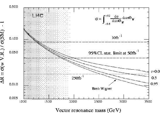
Figure 6.9: Excess of the signal as a function of the vector resonance mass. The vertical axis is the excess of the cross section in the given angular range normalized to the standard model cross section.

In this figure, the solid lines correspond to the Breit-Wigner resonance formula and those calculated based on the N/D method with $r=0.0,0.5$, and 0.95, respectively. The statistical limits at the 95% CL are shown by dashed lines for integrated luminosities of 10, 50, and 250 fb^-1. The shaded area is the region to be explored by the direct search at LHC[17]. We can see that JLC at $\sqrt{s}=500$ GeV with an integrated luminosity of 50 fb^-1 is sensitive to the vector resonance of mass up to about 2 TeV, which is similar to the sensitivity expected with the direct search at LHC. With five times more luminosity we may be sensitive to masses larger than 2.5 TeV. If we measure polarization of $W$ from angular analysis of decay daughters, higher sensitivity is obtained. Sensitivity based on the N/D method is shown in Fig.6.10.

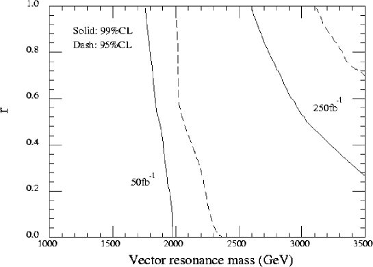
Figure 6.10: Contour plot of the sensitivity to the vector resonance based on the N/D method, in the plane of $r$ and the vector resonance mass.

In summary, the vector resonance in the $W_{L}W_{L}$ amplitude has significant effect at $\sqrt{s}=500$ GeV even if the mass of the resonance is as high as 2 TeV, and its effect can be observed at JLC.

Part III Detectors

Chapter 7 Interaction Region

7.1 Introduction

In this chapter we examine various aspects of experimentation that directly interacts with the accelerator design. Of particular concern in this area is the background to the physics experiments that are caused by the beams passing through the detector.

The characteristics of background events at JLC will be very different from those at typical $e^{+}e^{-}$ colliders, except the SLC. The features of the background strongly depend on numerous operational parameters of the accelerator, such as the beam aspect ratio (typically $\sigma_{x}^{*}/\sigma_{y}^{*}=0(100)$ ), a high beam intensity ($10^{10}$particles/bunch) and possible tails in the particle distribution that deviates from a Gaussian distribution. The population of low energy $e^{\pm}$ pairs that are created during collisions are directly related to the beam aspect ratio, while the tail is mostly responsible for synchrotron radiation and muon background. The optimization of the machine operational parameters must be considered by taking this “interaction” between the experimentation and the machine into account.

The highest-priority goal here is, of course, to maximize the luminosity while minimizing the background. With such a motivation in mind, the effects of $e^{\pm}$ pairs have been estimated by detailed Monte Carlo simulations with various configurations of masking system, in addition to simulations of synchrotron radiations and the attenuation of the muon flux that are produced by interactions of the beams with upstream collimator materials. Performances of luminosity monitor and active mask are demonstrated under the huge pair background. Preliminary design of dump line is also presented, where a possibility of beam-energy spectrum is discussed with an accuracy of $\leq 0.1$% and a beam loss is estimated for the major source of neutron-backgrounds at the interaction point(IP).

Another important issue is a stabilization of final quadrupole magnets to keep ”head-on” collisions between nano-meter beams. A detailed analysis of the support system is presented especially on the oscillation properties. A real-time measurement of the beam size is vital part of such a stabilization process. As the most promising detector, a pair monitor has been proposed and its expected performances are described.

7.2 Backgrounds

To illustrate where the background particles can originate, the beam line from the exit of the main linear accelerator (linac) to the interaction point (IP) is schematically shown in Figure 7.1. A $+7$ mrad bending magnet section (200 m long) downstream of the collimation section is needed in order to create a sufficient amount of separation for two experimental halls and to prevent the background from the upstream linac from directly hitting the detector. In the final focus system, beams are gradually deflected so as to have a horizontal beam crossing angle of $\pm 4$ mrad at IP.

There are two major sections for beam collimation (1200 m long) and a final focus system (1800m long) in the beam line to handle beam energies up to 0.75 TeV. While their main purposes are to clip the beam tails, secondary particles are inevitably produced, namely: (1) muons and (2) synchrotron radiation photons, respectively. In addition at the IP, (3) $e^{+}e^{-}$ pairs and (4) mini-jet are created through beam-beam interactions. They all cause background hits in the detector facility.

In subsequent sections the first three kinds of background are discussed together with a possible design of the interaction region.

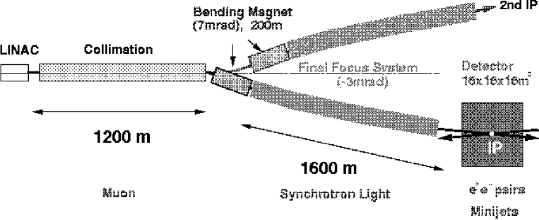
Figure 7.1: Top view of the beam line from the exit of the main linac to the interaction point (IP) at $E_{cm}=0.5-1.5$ TeV.

7.2.1 Collimation and Muons

In this section we discuss the production of muons through the interaction of particles in the beam tails when they are collimated at the upstream collimation sections.

Generally, the transverse profile of the beam does not exactly follow a Gaussian distribution at linear colliders. The beams can be accompanied by long tails according to experience from experiments at SLC [5]. While the origin of these tails is not thoroughly understood at present, we shall conservatively assume that the beam has a flat tail beyond $\pm 3\sigma_{x(y)}$ in both the horizontal(x) and vertical(y) directions with a relative intensity of $0.1\sim 1$%.

The beam must be collimated within $\pm 6\sigma_{x}$ and $\pm 40\sigma_{y}$ in order to keep the background due to synchrotron radiation at a manageable level. Since the typical size of the beam core is on the order of a few $\mu$m, collimating such beams is a seriously non-trivial task. A work-around is to expand only the tail part sufficiently by using a non-linear collimation technique, as discussed in Chapter 13. This is part of the reason why a 1200 m-long collimator section is required for collimating a 0.75 TeV beam.

One RF pulse will accelerate a bunch train which contains up to 95 bunches separated by 2.8 nsec at a repetition rate of 150Hz. Since each bunch consists of $7.5\times 10^{9}$ electrons (or positrons) at the IP, about $10^{8}$(1%tail)$\times 10^{2}$(bunches) electrons may hit collimators at 150 Hz. In the interactions of the beam tails with the collimators a large number of muons are produced through the Bethe-Heitler process, $e^{\pm}N\rightarrow e^{\pm}\mu^{+}\mu^{-}N$. Without suitable measures these muons would traverse through the tunnel and create a large amount energy deposit within the detector facility. They would cause serious background problems for conducting high-energy physics experiments.

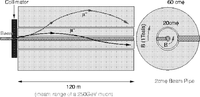
Figure 7.2: Original idea of a muon attenuator. Two iron pipes are magnetized axially in opposite directions for both charged muons, which can be trapped, where the 120m length of the iron pipe corresponds to a mean range of 250GeV muons.

There are eight collimators upstream of the big bend, which are located at 1840.3 $\sim$ 2855.6 m from IP as shown in Fig.7.3 (a). Two of them (col.-1 and -2) are set in the linac. They doubly collimate the beams in momentum space($\Delta p/p<\pm 2$%) and phase space of transverse profile and divergence ($6\sigma_{x}^{(\prime)}\times 40\sigma_{y}^{(\prime)}$). During the collimation, a lot of secondary particles would be produced. Among them high energy muons would create the most severe backgrounds. A rate of muons depends on a population in a tail of beam. For the conservative estimation, we assume that the tail is $0.1\sim 1$% of the bunch population for this simulation study.

In the simulation muons were tracked down to the detector of $16\times 16\times 16$m³ with various configurations of muon attenuation in a tunnel. The present simulation does not take account of optical elements except for bending magnets (Fig.7.3(a)) at the beam line. The muon attenuator is a magnetized iron cylinder of $1<r<30$cm, which actually comprises two cylinders of $1<r<10$cm (inner) and $10<r<30$cm (outer) as shown in Fig. 7.2. The axis of cylinders corresponds to the beam line. The two cylinders are magnetized circularly in opposite directions to confine positive and negative muons in each. The muon attenuator is assumed to cover from the big bend through the whole collimation system, which is 1510 to 2856m from IP. Figure 7.3(b) shows the number of electrons (e/$\mu$) at 8 collimators to produce one muon in the detector [7]. Open arrows indicate the lower limits since no muon was observed within the simulation statistics. The best configuration (solid triangles) was the muon attenuator magnetized at 10KG to confine positive muons ( 10 KG, $\mu^{+}$ inside ) in the inner cylinder, where the beam particles were 250GeV electrons. It attenuates muons by 4 order of magnitudes more than a case with no muon-shield (open circles). The oppositely magnetized attenuator( open triangles, 10 KG, $\mu^{-}$ inside ) has less shielding power than the best case for col.6-8 since the negative muons can be transported to the detector in the same way as the beam. The magnetization effect is clearly seen by comparing them with the no magnetized attenuator (solid circles, 0 KG). With the best configuration and the $0.1\sim 1$% beam tail, a few muons would hit the detectors per pulse for the pulse population of $(0.71\sim 1.33)\times 10^{12}$ corresponding to A$\sim$Y in Table 1.3. In this case the muons should not be a serious background.

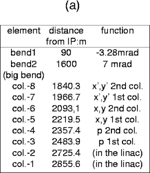
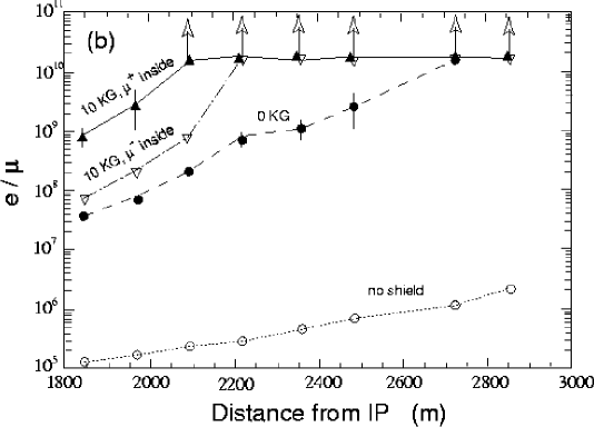
Figure 7.3: (a) Locations of bending magnets and collimators in the beam delivery system. (b) The number of collimated electrons (positrons), which give one muon in a detector of $16\times 16\times 16$m³, at eight collimators. Open circles are simulation results with no muon shield, and the others are those with muon attenuators at 1510$\sim$2856m from IP (Y. Namito, Jan.1999).

7.2.2 Synchrotron Radiation

Since the intensity of synchrotron radiation is on the same order as the intensity of the beam, itself, it would be very harmful to the experimentation if they are scattered at the pole tips of the nearest quadrupole magnet QC1. It is also very difficult to shield them near to the IP. The amount of synchrotron radiation is determined by the maximum size and angular divergence of the beam profile. Both the maximum beam size $(x,y)$ and the divergence $(x^{\prime},y^{\prime})$ shall be well defined and controlled by the collimators.

The divergences can be expressed by $\sigma_{\theta_{x(y)}}=\sqrt{\epsilon_{x(y)}/\beta_{x(y)}}$, where $\beta_{x(y)}$ is a (optical) beta function in the final focus system and $\epsilon_{x(y)}$ is an emittance of beams. The beam size and the divergence are related by $\epsilon_{x(y)}=\sigma_{\theta_{x(y)}}\cdot\sigma_{x(y)}$. If we can not control them by some means, we must change the optics to enlarge $\beta_{x(y)}$ so that $\sigma_{\theta_{x(y)}}$ decreases. We may thus even have to sacrifice the luminosity because of $\sigma_{x(y)}=\sqrt{\epsilon_{x(y)}\cdot\beta_{x(y)}}$. A similar situation would likely occur at the beginning of operation with a larger emittance than the expected one, as happened in the SLC experiments.

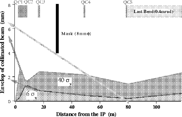
Figure 7.4: Horizontal(6$\sigma_{x}$) and vertical(40$\sigma_{y}$) beam envelopes through the last bending magnet and five final focus quadrupole magnets(QC1,QC2,QC3,QC4 and QC5). The maximum divergences of the synchrotron radiation are also drawn by arrows.

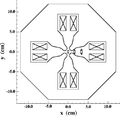
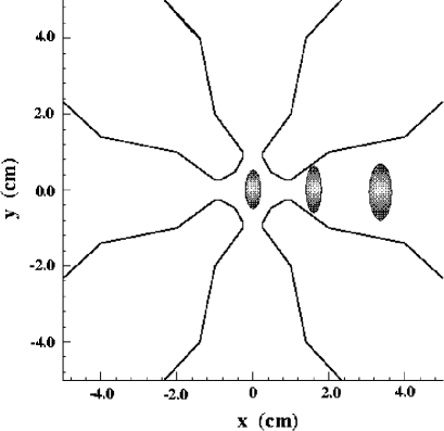
Figure 7.5: Profiles of the synchrotron radiation at QC1;right figure shows the magnified view around the center of QC1. The profile at the center accompanies the in-coming beam. The two right-hand side ones are passing through QC1 of 2.2m long after a collision with a 8mrad horizontal crossing.

Figure 7.4 shows the development of transverse beam envelops that correspond to $6\sigma_{x}\times 40\sigma_{y}$. Figure 7.4 covers the region from the IP up to the nearest dipole bend magnet. Here the smearing effect due to collimation is not taken into account, since it was estimated to be very small($10^{-8}$) as mentioned earlier.

With a mask of 8 mm$\phi$ radial aperture that is located at 30 m from the IP, synchrotron radiation from upstream magnets beyond the last bending magnet can be completely masked. Any synchrotron radiation that passes through the aperture of 8 mm$\phi$ mask would pass through the final quadrupole magnet (QC1) without scattering. The half aperture of QC1 is chosen to be 6.85 mm. As can be clearly seen in Figure 7.4, the radiation from QC3 and QC2 provides the maximum divergence at the IP in the horizontal and vertical directions, respectively. The profiles of the radiation at the QC1 are shown in Figure 7.5. The length and inner aperture of QC1 are 2.2 m and 13.7 mm$\phi$, respectively. The front face of QC1 is located 2.0 m from the IP. The in-coming radiation passes through the central axis of QC1. After colliding with the opposing beam at a horizontal crossing angle of 8 mrad, the out-going radiation passes off-axis through the QC1 magnet on the other side. The location of the out-going radiation is depicted as two elliptic profiles on the right-hand side of Figure 7.5.

As described above, it is expected that there should be no background problems due to the synchrotron radiation if we carefully optimize the collimation and the optics simultaneously.

7.2.3 $e^{+}e^{-}$ pairs

An enormous amount of $e^{+}e^{-}$ pairs will be created during collisions, for instance a few times $10^{5}$ pairs per bunch crossing. While their vast majority are scattered into extremely forward angles, some can be greatly deflected by the strong magnetic field that is produced by the in-coming beam. In such cases they can enter the detector region and can create background noise to the detector facility.

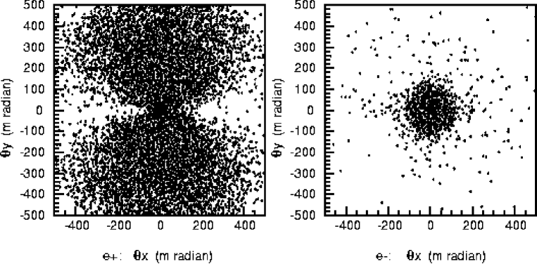
Figure 7.6: Electrons and positrons scattered by beam-beam interaction at IP. The vertical and horizontal axes denote the scattering angles in the vertical and horizontal directions, respectively. The left- and right-hand figures show the distributions of the positrons and electrons, respectively, downstream of the electron beam. Since the positrons have the same sign charge as the in-coming (positron) beam, they are scattered by larger angles than the electrons.

Figure 7.6 shows the angular distributions of pair-produced electrons and positrons after the beam-beam interaction. The calculation was made using ABEL[9]. Many particles (electrons or positrons) are scattered at large angles exceeding 200 mrad. We can also clearly see an asymmetry in their azimuthal distribution. More particles are deflected in the vertical direction than in the horizontal because of a very flat transverse beam profile ($\sigma_{x}^{*}/\sigma_{y}^{*}=260{\rm nm}/3.0{\rm nm}$). Since the energies of the particles are relatively small, and are at a few hundreds MeV, most of these particles are confined near the beam axis due to the detector solenoid magnetic field. However, when they hit QC1 in the out-going side, many secondary photons are back-scattered uniformly into the detector region. They can become serious background.

7.3 Layout

IP layout is shown in Fig.7.7. Nearest final quadrupole magnet (QC1) is located at 2m from IP, where the QC1 is shielded against a solenoid field of 2 Tesla by a superconducting compensation magnet.

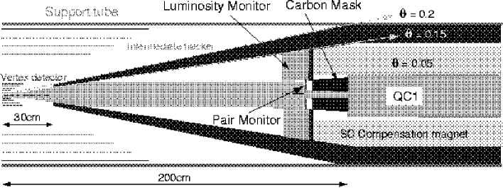
Figure 7.7: Interaction region.

A huge number of X rays, which are created in electromagnetic showers of $e^{\pm}$ pairs at QC1, are absorbed in conical and cylindrical tungsten masks. Angular coverage of the conical mask ranges from 0.15 to 0.2 radian, leaving a small dead cone angle, but the front part of the conical mask could be instrumented as a calorimeter. There is the luminosity monitor covering an angular region between 0.05 and 0.15 radian inside the mask. The carbon mask in front of the QC1 is very effective to absorb low energy back-scattered electrons. The 4-layer vertex detector (VTX) is located at radial distance from 2.4 to 6.0cm, followed by an intermediate tracker to link charged tracks between the central drift chamber (CDC) and the VTX. All these instruments are installed in a support tube of 80cm diameter[10].

The interaction region has been updated since the 1st ACFA-LC (Beijing) workshop[11] in order to further reduce $e^{\pm}$ pair backgrounds in VTX and CDC, especially X-rays in the CDC. The major changes are in the beam pipes and the locations of the carbon mask and the pair monitor. The beam pipe inside the VTX is made of 0.5mm thick beryllium, 4cm in diameter, while the major part is a 15cm diameter beam pipe of 2mm thick aluminum in the mask. These two beam pipes are connected with a conical beryllium pipe of 2mm thickness. The 15 cm diameter is large enough for $e^{\pm}$ pair particles to curl inside the beam pipe without interactions. The pair monitors consisting of active pixel device are now located at 176cm from IP, i.e. inside of luminosity monitor. In the previous design, they were closer to IP and were one of the sources of X rays.

7.4 Estimation of background hits

7.4.1 $e^{+}e^{-}$ pairs

There is a desire to increase the detector magnetic field ($B$) from 2 to 3 Tesla. The motivations are to reduce backgrounds and to place a vertex detector closer to beam line as well as to reduce the overall detector size. We study a case of $B=$3Tesla in terms of backgrounds in two major detectors, which are CDC filled with 1atm CO₂/isobutane (90%/10%) and VTX of $25\times 25\mu$m² pixels. Inner and outer radii of the CDC are 0.45 and 2.3m, respectively, and the length is $\pm 2.3$m. The VTX is assumed to be consisted of three layers ( r=2.5, 5.0, 7.5 cm and z=$\pm 7.5,15.0,22.5$cm, respectively) in this study. Background hits were also simulated with detailed geometries by JIM, where photons and electrons(positrons) are tracked down to their energies of 10keV and 200keV, respectively.

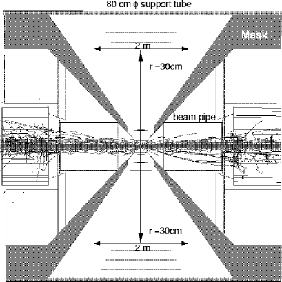
Figure 7.8: Pair samples in the support tube at $B=$2 Tesla by JIM simulation, where photons of $>100$MeV and electrons(positrons) of $>10$MeV are only shown for display purpose.

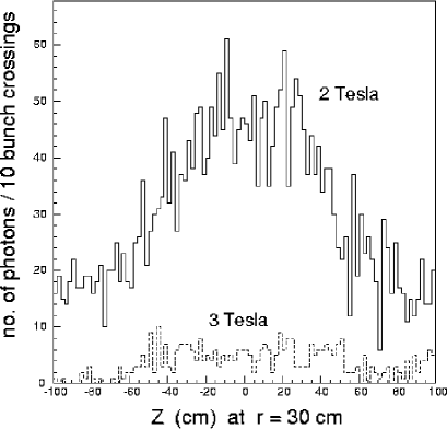
Figure 7.9: Number of photons traversing a cylinder of 60cm$\phi\times\pm$ 100cm long as a function of z at $B=$2 and 3 Tesla for the CDC background estimation.

The major backgrounds are secondary photons in the CDC although the CDC is shielded against them by the masks. For an estimation of the photons entering the CDC, we counted the number of photons traversing a surface of 60cm$\phi\times\pm 1$m long cylinder. Figure 7.9 shows the results at $B=$2 and 3 Tesla for 10 bunch crossings. Most of the photons are created by low energy electrons (or positrons) hitting the 4cm$\phi$ beam pipe very near IP . We can see an apparent advantage of higher magnetic field in Fig.7.9 because of stronger confinement of the electrons(positrons) around the beam line at $B=$3 Tesla. On the other hand, the main backgrounds to VTX are primary electrons(positrons).

Table 7.1: Pair backgrounds for 4cm$\phi$ beam pipe at $B=$2 and 3 Tesla for beam parameters of the basic JLC-A(95 bunches/train) and the high luminosity option of JLC-Y(190 bunches/train), where numbers are for 10 bunch crossings if there is no specification.

	r	z	B =	2 Tesla	B =	3 Tesla
	cm	cm	JLC-A	JLC-Y	JLC-A	JLC-Y
photons	30	$\pm$100	3076	6082	371	946
vtx-1:hits	2.5	$\pm$7.5	2186	3279	900	1205
/mm2/train			0.9	2.8	0.4	1.0
vtx-2:hits	5.0	$\pm$15.0	720	920	104	306
vtx-3:hits	7.5	$\pm$22.5	406	545	34	138
CDC:hits(tracks)	45$\sim$230	$\pm$230	121(101)	235(194)	12(9)	37(28)

Rates of background hits are summarized both at $B=$2 and 3 Tesla in Table 7.1. As mentioned above, the backgrounds hits in CDC are proportional to the numbers of photons, which are one order of magnitude less at $B=$3 Tesla than those at $B=$2 Tesla. The CDC hit rates were estimated to be 1210 and 120 hits per a train crossing at $B=$2 and 3 Tesla, respectively. Assuming that the total number of CDC readout channels is 10000, corresponding occupancy rates are 12 and 1.2 % at $B=2$ and 3 Tesla, respectively. In the VTX the most severe backgrounds were observed at the innermost layer, where the hit densities are estimated to be 0.9 and 0.4 /mm²/train at $B=$2 and 3 Tesla, respectively. We also simulated backgrounds for the case of the high luminosity option specified as JLC-Y. The results are also listed in Table 7.1. For the JLC-Y, the background rates per bunch crossing increase by 1.3$\sim$3 times because of smaller beam sizes as seen in Table 1.3. Doubling the number of bunches per train crossing at the JLC-Y, the CDC occupancy and the VTX hit density can be estimated to be 47 (7.4)% and 2.8(1.0)/mm²/train, respectively, at $B=$2 (3) Tesla.

Setting background tolerances for 10% occupancy and 1/mm²/train hit density in the CDC and VTX, respectively, the backgrounds with $B=2$ Tesla are marginal at the JLC-A and they may overwhelm the detectors at the luminosity-upgraded JLC-Y. For the case of $B=3$ Tesla, there seems to be a possibility of placing the VTX closer to the beam line at least for the JLC-A. Therefore two configurations of the VTX and beam pipe have been studied by the JIM simulation. The first comprises the VTX of 1.5cm minimum radius ($r_{vtx1}$) and 2cm$\phi$ beam pipe, while the second comprises the VTX of $r_{vtx1}$=1.8cm and 3cm$\phi$ beam pipe. Radii of the second and third layer of the VTX are 2.5cm and 5.0cm, respectively, for both configurations. The simulation results are summarized in Table 7.2. From the point view of the background tolerances, the second configuration is only allowed for the CDC occupancy of 7.2% and the VTX hit density of 1.6/mm²/train. At the JLC-Y, a more elaborate study shall be needed on a detailed geometry of beam pipe as well as a tracking algorithm in the CDC with the ”exceeded” occupancy even if the innermost layer of the VTX may be overwhelmed by backgrounds.

Table 7.2: Pair backgrounds for 2 and 3 cm$\phi$ beam pipes at $B=$ 3 Tesla for the JLC-A, where numbers correspond to 10 bunch crossings if there is no specification.

	r	z	B =	3 Tesla
	cm	cm	2cm$\phi$	3cm$\phi$
photons	30	$\pm$100	5857	1626
vtx-1:hits	1.5	$\pm$4.5	3065	-
/mm2/train			3.6	-
	1.8	$\pm$5.4	-	1906
/mm2/train			-	1.6
vtx-2:hits	2.5	$\pm$7.5	680	804
vtx-3:hits	5.0	$\pm$15.0	402	208
CDC:hits(tracks)	45$\sim$230	$\pm$230	259(217)	72(63)

7.4.2 Neutrons

We estimated the neutron background produced through photo-nuclear reaction. The pair background particles hit the QC1 and make the EM shower, and the photons in the shower cause the photo-nuclear reaction. The neutrons produced here can spread over the entire detector inside the iron structure.

The pair background particles which can go through the QC1 cannot be transported along the same line as the main extracted beam and will hit the components of the extraction beam line resulting the EM shower. The beamstrahlung photons have the very small angular divergence but eventually hit the beam-dump and also produce neutrons. These neutrons can come back to the IP region through the hole for the beam pipe.

In order to study the neutron background produced at the QC1, we used a computer code written by Dr.T. Maruyama at SLAC for the neutron generation built into GEANT3. For the neutron transportation in GEANT3, FLUKA(for $E_{n}>20$ MeV) or MICAP(for $E_{n}<20$ MeV) was used. The cut-off energy for neutral hadrons was 1 keV. We counted the number of neutrons passing the z = 0 plane in the simulation. We found 66 neutrons passing the plane in r $<$ 10 cm area for 1000 bunch crossing. This number corresponds to $3\times 10^{7}/$cm²y near interaction point. As the main tracker the central drift chamber (CDC) with gas mixture of CO₂:Isobutane(C₄H₁₀)=90:10 is being considered. Since this gas mixture contains hydrogen atoms, neutrons can make background hits by elastic scattering. The number of the background hits in the CDC we obtained by the simulation is 800 hits/train.

We have also estimated neutron backgrounds using Fluka98 program. In this calculation, we used the magnetic field consisted of the detector solenoid of 2 Tesla, the QCS magnets, and the compensation magnets to cancel out the solenoid field in QCS region. In this configuration, the magnetic field vector which points along beam direction at IP region changes the direction to perpendicular to the beam axis. Since the Z components of the magnetic field which could trap soft $e^{\pm}$ was reduced, more $e^{\pm}$ hit the inner surface of QCS. However, neutrons which returned to IP were produced mostly at the front surface of QC1, the large increase of neutron yield by this effect was not observed.

In FLUKA simulation, the cut off energy for neutron transport was 1 keV while those for $e^{+}/e^{-}$ and photons were 10.511 MeV an 4 MeV, respectively. As seen in Fig. 7.10, the only few neutron had energy less than 10 keV.

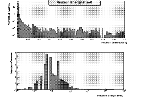
Figure 7.10: The energy spectrum of neutron which return to at IP. Note that the scaling of upper and lower figure is different: Upper figure is log Y scaling, and lower figure is log X scaling.

From the Fluka simulation, we obtained the number of neutron distribution at Z=0 as shown in Fig. 7.11. From this figure we got the total number of neutron within the radius of 10 cm is 292 for 1000 bunch crossing (BX) ( entries in the figures are doubled to count backgrounds by $e^{-}$ and $e^{+}$). If uniform neutron distribution is assumed the average neutron flux is $0.93\times 10^{-3}$ $n/{\rm cm}^{2}$ per bunch crossing. For 1 year ( $10^{7}$sec ), we get $13\times 10^{7}$ $n/cm^{2}/year$ at IP. The result is consistent with the GEANT3 simulation within a factor of 4, if we neglect a difference of magnetic field distribution used for the simulations.

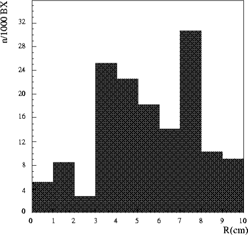
Figure 7.11: The number of neutrons as a function of radius at Z=0 (IP). The vertical axis is scaled so that it gives the number of neutron for 1000 bunch crossing.

At present it is difficult to make a reliable estimation on the neutron background from the downstream because we don’t have the design of the beam extraction line of the JLC yet. So we made a very rough estimation on it. By the detector simulation it was found that among the total energy of 100 TeV of the pair background particles in one bunch crossing, 13 TeV is absorbed in the QC1 and 87 TeV goes downstream. By scaling the neutron background from the QC1 with the deposited energy, we get the upper limit of the neutron background produced by pair background particles at the QC1 and other beam line components downstream of the QC1 as $1.5\times 10^{7}\times 100$ TeV/13 TeV $\sim 1\times 10^{8}/cm^{2}/year$.

For the estimation of the neutron background from the beamstrahlung photons, we assumed all photons lose their energy in the water beam dump located at 300 m from the IP. The electron/positron beam was assumed to be bent before the water beam dump and dumped elsewhere so that the neutrons from the $e^{\pm}$ dump can be shielded sufficiently.

Using the GEANT3 simulation with the neutron generation code we found that $6\times 10^{20}$ neutrons are produced in one year which is reduced to $1\times 10^{17}$ at the surface of the beam dump on the IP side owing to the self shielding by the water. If the solid angle acceptance at the IP is simply multiplied, the resulting neutron yield at the IP is $2\times 10^{7}n/cm^{2}/year$.

According to the Fluka98 simulation, the neutron yield at the surface of water dump is $2.8\times 10^{17}$ neutrons per year which corresponds to $5\times 10^{7}n/cm^{2}/year$ at IP if we take into account the acceptance of solid angle and contribution from two water dumps are added.

7.5 Background hits in different detector models

So far the final focus quadrupole magnets(QC1) are assumed to be located 2 m away from the interaction point($l^{*}$=2 m). Recently a new idea of final focus optics is proposed [12] which makes longer $l^{*}$ of 4.3 m possible. With this optics, the background particles ($\gamma$, $e^{\pm}$, neutron) due to back-scattering from QC1 would be reduced. In this section, we present the results of simulation studies on the pair-background in several detector models which have different magnetic field, mask design, and $l^{*}$.

Background hit rate has been studied for four detector models (table 7.3). The layout and background estimations in the previous sections are based on 2 T model [1]. Compared with the 2 T model, the outer radius of the central drift chamber (CDC) and inner radius of the barrel calorimeter of the 3 T models are reduced in order to keep the minimum $p_{t}$ of charged particles which reach the barrel calorimeter constant. The length in $z$ direction of the CDC and the $z$ position of the endcap calorimeter are also reduced in 3 T models. In models a) and b), large conical tungsten masks are placed to shield the back-scattered particles produced by the pair-background particles hitting the QC1 as shown in Fig.7.7. Instead, smaller conical masks are used for the model c). Model d) is for the case of $l^{*}$=4.3 m. Two sets of forward calorimeters work as active masks in this model. Schematic views of model c) and d) are shown in Fig. 7.12. The pair-background particles were generated using a program code CAIN [13] for the JLC-A. These particles were put into a full detector simulation program JIM which is based on GEANT3. Magnetic fields of the QC1 and the compensation magnets were taken into account. The cut-off energy was set to 10 keV for $\gamma$’s and 1 keV for neutrons.

Table 7.3: Detector models and expected background hits per beam crossing: track density at the innermost layer ($r$=$24$ mm) of vertex detector(VTX), a number of hits in the central tracker(CDC) by $\gamma$ and neutron, and an energy deposit in calorimeter(CAL), where models a) and b) are called as 2 T model and models c) and d) are called as 3 T model.

Model	$B$(T)	$l^{*}$(m)	Mask	VTX($/{\rm cm}^{2}$)	CDC($\gamma$)	CDC(n)	CAL(MeV)
a	2	2	150 – 200 mrad	0.7	2	30	600
b	3	2	150 – 200 mrad	0.4	1	2	900
c	3	2	70 – 100 mrad	0.4	2	2	900
d	3	4.3	–	0.4	1	0.1	30

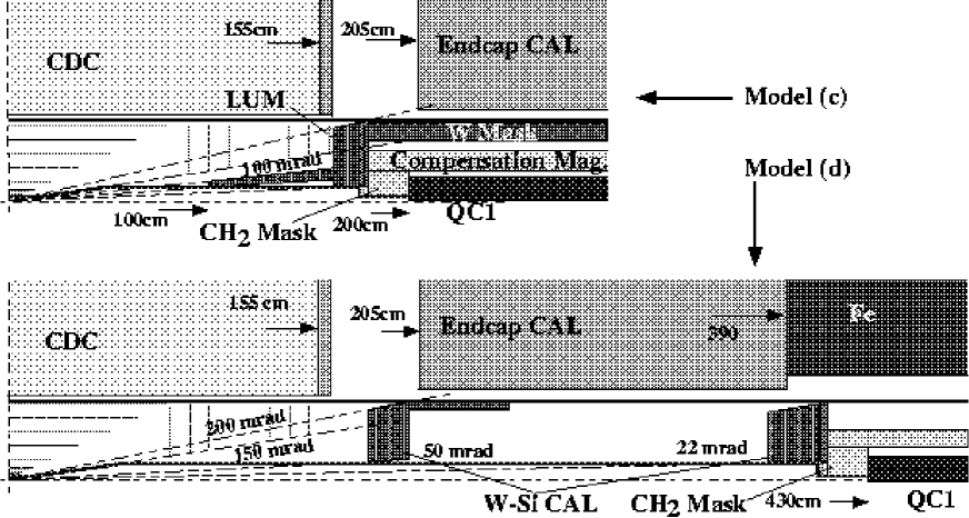
Figure 7.12: Schematic views of model c) and d) detectors in the 3 T model.

The results of the simulation are given in table 7.3. Background hit rate of CDC by neutrons in the 2 T model is quite high because 10 cm thick tungsten mask is not enough to stop neutrons. In the 3 T models, the CDC hit rate by neutrons is reduced because the neutron source (QC1) is surrounded by the endcap calorimeter which works as a neutron shield. With $l^{*}$=4.3 m optics, the background source is located farther from the detector components and the background hit rate of the detectors get even less. The simulation was also performed with the JLC-Y. The result shows about two times more background, while the luminosity is 3 times more than that of the JLC-A.

7.6 Pair monitor

The disk-shaped pair monitor comprises double layers of active pixel sensors whose pixel size and thickness are $100\times 100\mu$m² and 300$\mu$m of silicon, respectively. The inner and outer radii are 2 and 8.5cm, respectively. The pair monitor should measure positions and energy deposits of electrons or positrons and secondary photons.

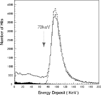
Figure 7.13: Energy deposits in the pair monitor. The solid and dashed histograms show energy deposits in each cell and those by a track, respectively. The black one show those of secondary backgrounds in each cell.

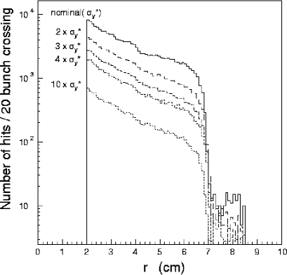
Figure 7.14: Hit distributions normalized at 20 bunch crossings as a function of $r$ for energy deposits of $>$70keV, where histograms correspond to 5 vertical beam sizes at IP; i.e. basic ($\sigma^{o}_{y}$), $2\times,3\times,4\times$ and $10\times\sigma^{o}_{y}$

.

Figure 7.14 shows the energy deposits simulated with detailed geometries by JIM, where the pairs have been generated with beam parameters of JLC-A by CAIN21d[13]. Many of them hit only one cell and, as clearly seen in this figure, a very sharp peak appears around 100keV. Therefore, they can be effectively discriminated from the secondary backgrounds simply by a 70 keV threshold in energy deposits.

In order to see how we can measure the beam sizes, pairs have been generated with five different vertical beam sizes at IP by CAIN[13], i.e. $\sigma_{y}=\sigma_{y}^{o}$(basic), $2\times\sigma_{y}^{o}$, $3\times\sigma_{y}^{o}$, $4\times\sigma_{y}^{o}$ and $10\times\sigma_{y}^{o}$ for the statistics of 20, 40, 60 50 and 110 bunch crossings, respectively, while the other beam parameters are the same as the basic ones. The minimum energy of the pair particles was 3 MeV.

Radial distributions of the pairs are shown in Fig.7.14, where the number of hits are normalized at 20 bunch crossings for realistic statistical comparisons. All five histograms have sharp shoulders, while negligibly small tails are due to those scattered inherently at large angles. As clearly seen in this figure, positions of the shoulders do not depend on the vertical beam size($\sigma_{y}$) indeed as described in  [14]. Since they depend on the horizontal beam size($\sigma_{x}$) as well as well-known beam intensities, the horizontal beam size can be estimated by the radial distribution.

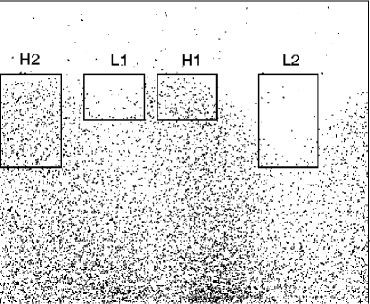
Figure 7.15: Scatter plot of hits with $>$70 keV energy deposits in the pair monitor on a plane of azimuthal angle(x) and radial position (y), where four sensitive areas are also depicted in order to calculate a ratio of $(L_{1}+L_{2})/(H_{1}+H_{2})$

.

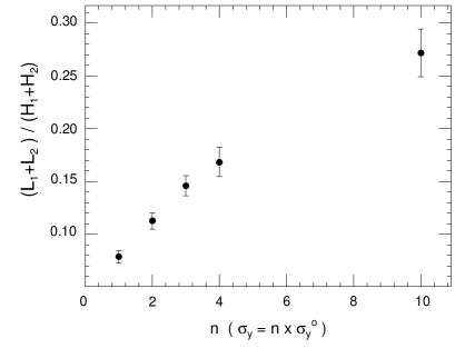
Figure 7.16: Ratio of $(L_{1}+L_{2})/(H_{1}+H_{2})$ as a function of vertical beam size ($\sigma_{y}=n\times\sigma^{o}_{y}$) at IP, where error bars are statistical corresponding to 20, 40, 60, 50 and 110 bunch crossings for n=1,2,3,4 and 10, respectively.

The most interesting observable is the distribution of azimuthal angles, since the angles carry an information of the vertical beam size as a function of aspect ratio,$A\equiv\sigma_{x}/\sigma_{y}$. Among the pair particles, particles of the same charge as the incoming beam must be deflected with large angles because of repulsive Coulomb forces. When the incoming beam has a large aspect ratio, the particles are scattered asymmetrically due to the asymmetric Coulomb potential, that is, more vertically than horizontally. Figure 7.16 shows a scatter plot of hits in the pair monitor on a plane of azimuthal angle and radial position. Two dense bands can be seen, which are made of particles deflected upward or downward and swum helically in the 2 Tesla solenoid field. In order to quantify the asymmetry, we set four regions ($H_{2},L_{1},H_{1},L_{2}$) as shown in Fig.7.16. Area of $H_{2}$ and $L_{2}$ is larger than that of $H_{1}$ and $L_{1}$ because of left-right asymmetry with 8 mrad crossing angle. Then, we defined a ratio, $R\equiv(L_{1}+L_{2})/(H_{1}+H_{2})$ as proposed[14], where $L_{1},L_{2},H_{1},H_{2}$ represent the number of hits in each region. It is expected that $R$ becomes smaller as $A$ increases while $R=1$ for round beams. The simulation results are shown for beams with five different $\sigma_{y}$’s in Fig.7.16. Up to $4\times\sigma_{y}^{o}$, we observed a linear relation between R and the vertical beam size. Under the basic beam condition, the vertical beam size could be measured for 100 bunch collisions with $<10$% statistical accuracy. Since this method, i.e. counting hit numbers in specific regions with energy deposits of greater than 70 keV, is very simple, the pair monitor can be a feedback device for beam tuning in realtime. With the fast gate, the pair monitor should detect the pairs in specific bunches in order to investigate a variance of beam size in a bunch-train.

7.7 Luminosity Monitor and Active mask

Luminosity monitor is located at 163cm from the interaction point (IP), which is made of tungsten (W) of 15cm thickness (42.86$X_{o}$) and the (polar) angular coverage ranges from 0.05 to 0.15 radian. It is segmented into 32, 16 and 128 divisions in radius (r), azimuthal angle ($\phi$) and longitudinal coordinate (z), respectively. The physical dimensions are 5mm, 3.2-9.7cm and 1.17mm in r, $\phi$ and z, respectively. At present, all the tungsten segments are treated as sensitive detectors; that is, energy deposits in all segments are calculated in simulations. A real detector must have some sensitive layers made of active material such as scintillator, silicon pad, or crystal (e.g. BGO) instead of tungsten.

A front part of the conical mask is instrumented to measure energy deposits in electromagnetic showers. The mask is made of tungsten. The longitudinal position is 30cm from IP and the angular coverage is from 0.15 to 0.2 radian. The active mask consists of 8 layers of silicon pads ( Si(200$\mu$m) + G10(300$\mu$m) ), where the first W layer is 5mm thick and the other W layers are 1cm thick. In simulations, energy deposits in silicon pads are calculated. The active mask is segmented into 8-10 and 32 divisions in r and $\phi$, respectively. The physical dimensions are 2mm and 0.9-1.2cm in r and $\phi$, respectively.

The $e^{+}e^{-}$ pairs were generated with a statistics corresponding to 100 bunch crossings ($\sim$1 train crossing) by cain21d, where the nominal JLC-A machine parameters at $\sqrt{s}$=500GeV were used. They should always overlap on any physics event at JLC. For the signals, electrons of 50 or 250GeV were generated into the front center of the luminosity monitor and the active mask. Their energy deposits were calculated by the JIM simulation, and they are listed in Tab.7.4

Table 7.4: Energy deposits in the luminosity monitor (LM) and active mask (AM) per 100 bunch crossings.

$B$=2T	$e^{+}e^{-}$ pairs	50GeV $e$	250GeV $e$	250GeV $\mu$
AM	264MeV	120.4MeV	541.0MeV	0.48MeV
LM	152GeV	49.9GeV	249.5GeV	1.67GeV
$B$=3T	$e^{+}e^{-}$ pairs
AM	29.3MeV
LM	46.7GeV

,where energy deposits due to 250GeV muons are also listed. As clearly seen, energy deposits of $e^{+}e^{-}$ pairs decreases at higher magnetic field ($B$=3T). The luminosity monitor contains all electromagnetic shower while the active mask has shower leakage of $\sim$10% in radial direction for a 250GeV electron compared with a 50GeV electron. The longitudinal leakage in the active mask with 21.4$X_{o}$ was estimated to be $\sim$1% even for a 250GeV electron.

Although the total energy deposits of $e^{+}e^{-}$ pairs are very large, the spatial distributions are very different from those of electrons as seen in Fig. 7.17 and  7.18 for LM and AM, respectively. The simulations show that most of the pairs are absorbed near the surfaces of $\sim 1X_{o}$ depth because of their low energies while the 50GeV and 250GeV electrons have shower maxima at 5$X_{o}$ and 8$X_{o}$, respectively.

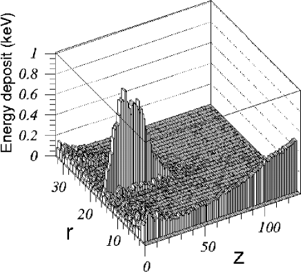
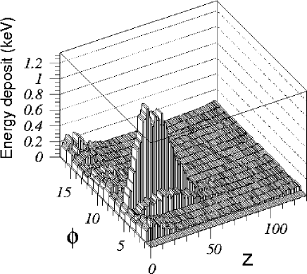
Figure 7.17: Energy deposit of a 50 GeV electron together with $e^{+}e^{-}$ pairs whose statistics corresponds to 100 bunch crossings in LM. Left and right figures are plotted in r-z and $\phi$-z planes, respectively.

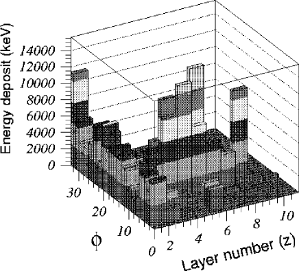
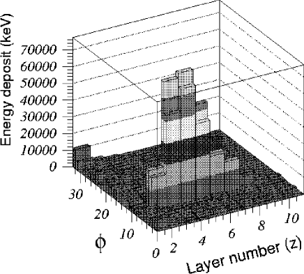
Figure 7.18: Energy deposit of a high energy electron together with $e^{+}e^{-}$ pairs whose statistics corresponds to 100 bunch crossings in AM. The electron energies are 50 and 250 GeV in left and right figures, respectively.

Among the total energy deposit of 152 (46.7) GeV/train in LM due to $e^{+}e^{-}$ pairs, only $54^{*}(14^{*})$ GeV comes from the front at B=2(3)T, while most comes from the inner-back. (^∗ sum of incoming energies). The $\phi$-segmentation (16 div.) is important for angular resolution, and the r-segmentation (32 div.) is desired to determine polar angle with an accuracy of a few milli-radian. So, a fine-segmented W/Silicon calorimeter seems to be ideal. The thickness of tungsten layers must be optimized for energy-resolution.

For AM, first layer (5mm thick W) has $\sim$50% energy deposit for $e^{+}e^{-}$ pairs. Again, $\phi$ segmentation (32 div.) is important for angular resolution. Eight layers of W/Si-pad calorimeter (21.4$X_{o}$) works very well for vetoing high energy electrons.

7.8 Support system

To support the components at the interaction region, 80 cm diameter with 10mm thick of support tube made of CFRP was proposed. The support tube is usually acted on self-weight of the components and vibrations from the ground. One of the important requirements is that relative displacement between QC1 separated by 4 m has to be kept less than 1 nm. Therefore, to optimize the support tube configuration, static analysis and dynamic analysis were carried out. And to realize these analyses, the excitation test using prototype model is being done.

At the initial concept of support tube, 12 m long single CFRP tube is provided and it is supported on the both of iron end yokes. Analysis in terms of this configuration was studied and reported at the 2nd ACFA-LC workshop in Seoul. It showed that relative displacement to be excited by ground motions were completely negligible between QC1’s. Since then, a new analysis has been executed on a system, where the two final focus doublets are independently supported by two identical cantilevers. If the system is stable in terms of ground motions, it is experimentally more preferable because of less material in detectors as well as easier assembling of the doublets and more straightforward installation.

In the calculations for the support tube, stiffness of the support tube was ignored. The bending stiffness can be defined to D=EI, where D is the bending stiffness, E is Young’s modulus and I is moment of inertia. Moment of inertia is proportional to $10^{4}$ of the thickness. Thus, compared to the bending stiffness between 10mm thick of CFRP support tube and tungsten mask, stiffness of the tungsten mask is to be 25 times larger. So, only the stiffness of the 10 cm thick tungsten mask was taken into account. The tungsten mask consists of 4 pieces in the longitudinal direction and 2 pieces in the circumferential direction as shown in Fig. 7.19. Overall length after assembling is 8 m and load conditions are self-weight of 32 tons for tungsten mask and other components of 9 tons, respectively. The mechanical properties of tungsten are, Young’s modulus is 415 GPa, density is 19.3 and tensile strength is 900 MPa, respectively.

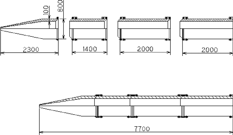
Figure 7.19: Configuration of the tungsten mask.

Figure 7.20 shows the results of static analysis. The gravitational sag due to load of 41 tons was calculated to be 1.6 mm at the top of tungsten mask when it assumed that the tungsten mask is fixed to two points where 7 m far and 8 m far from the interaction point. Stress level was to be 23 MPa that is sufficient low against the tensile strength. This deformation is not accepted. If the mask is additionally fixed at 3.85 m far from the interaction point, the gravitational sag can be improved to 0.09 mm. This indicates that the mask is supported at the back end and the iron yoke.

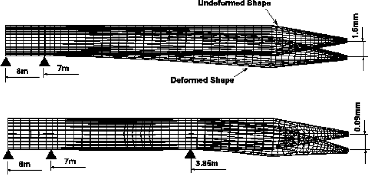
Figure 7.20: Deformation of the tungsten mask due to a load of 41 tons.

To know the behavior against vibration such as ground motion, dynamic analysis was carried out. Kinds of dynamic analysis are modal analysis to know the natural frequency and mode shape of structure, harmonic response analysis to know the amplitude at the resonant frequency and spectrum analysis to know the amplitude by input the combined different vibration characteristics. In the dynamic analysis, two analysis models were assumed. One is the support is fixed to the rigid base so called “rigid case”. And the other is the support is fixed to the soft base whose natural frequency is 15 Hz, “soft case”. Usually, natural frequency of large structure is supposed to be relatively low, and from the viewpoint of the seismic design, natural frequency of large structure is to be around 15 Hz. Constraint points are 3 points where 3.85m, 7 m and 8 m from the interaction point, respectively.

As shown in Fig. 7.21, the result of modal analysis on the rigid case is calculated to natural frequency of 71 Hz at first mode, 179 Hz at second mode and 202 Hz at third mode, respectively. In the soft case, natural frequencies are calculated to be 15 Hz at first mode, 54 Hz at second mode and 93 Hz at third mode, respectively.

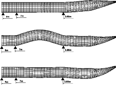
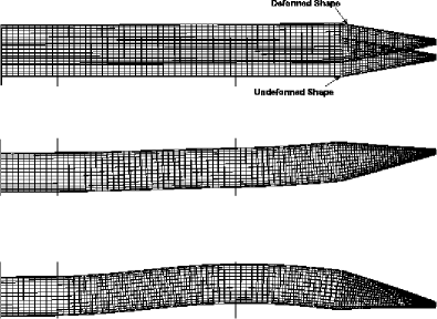
Figure 7.21: Mode shapes by the modal analysis at the first, second and third natural frequencies. Left and right figures show rigid and soft cases, respectively.

As the next step of dynamic analysis, harmonic response analysis was done. This calculation is a technique used to determine the steady-state response of structure to loads that vary harmonically with time. Applied acceleration was determined from data of grand motion measured in the TRISTAN tunnel. Correlation of amplitude and frequencies are 3 $\mu$m at 3 mHz, 1 $\mu$m at 0.1 Hz, 10 nm at 1 Hz and 5nm at 3 Hz, respectively[15]. From these data, acceleration forces can be converted to $1\times 10^{-7},4\times 10-^{4},4\times 10^{-5}$ gal and $2\times 10^{-4}$ gal, respectively. So acceleration force of $2\times 10^{-4}$ gal was chosen because of the largest value. Dumping ratio was set to 2 %. The calculation results of the rigid case is about 0.2 nm as shown in Fig. 7.22. Responded deformation at the soft case is to be 6 nm.

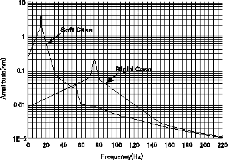
Figure 7.22: Results of the harmonic response analysis , where peaks are at the first natural frequencies.

At the spectrum analysis, three kinds of measured amplitude are input to the constraint points, and then vertical deformations at each resonant frequency are calculated. Figure 7.23 shows the calculation results. The deformation of rigid case at each mode is calculated to be from 3 nm to 8 nm. The soft case was turned out to be more stable then the rigid case since the structure was so rigid that it would not be deformed locally. For the soft case, the largest movement was smooth shift by $2.5\pm 0.2$ nm at the first mode of 15Hz. Good coherency of ground motions has been observed at such short distance between two points in many places. Therefore, the results are encouraging. Since the coherency generally diminishes at higher frequencies, an oscillation proof must be essential for the support system at $f\geq 10$ Hz.

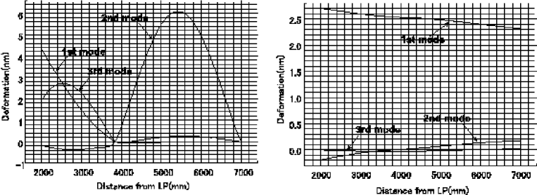
Figure 7.23: Deformations of the tungsten mask between 2 and 7 m from IP by the spectrum analysis. Left and right figures show rigid and soft cases, respectively. Mode shapes are similar to those of the modal analysis.

Vibration test using prototype model is just in process. The main purpose is to evaluate a validity of calculations by measuring oscillation properties of the prototype model. In the prototype model design, natural frequency resembles to the real support tube as possible. Two kinds of prototype models are provided those are cantilever type and both ends fixed type. Size of the prototype model is 800mm long and square aluminum bar(100 mm wide and 20 mm thick). They are excited by maximum strength of 10kg long stroke shakers. Input signals are provided by manual sine controller. In the test, some study items are planed; (a) measurement of natural frequencies and amplitudes of the oscillations, (b) measurement of amplitudes with different phases at both ends, (c) comparison between both-ends and cantilever support cases, (d) effects of supporting methods, that is, number of bolts and its sizes (e) measurement of dumping coefficients. Configuration of the data taking as shown in Fig. 7.24 is two laser position meters are set to the fixed end and free end of the bar, and velocity sensor (Geophone) and G-sensor are placed on the fixed end. Then those data is taken by the data logger and they are sent to the PC computer. Data from Geophone can be analyzed by FFT too.

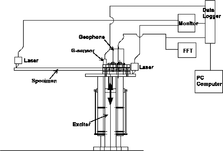
Figure 7.24: Test configuration of the prototype in a cantilever case.

7.9 Dump line

Preliminary design of the dump line, beam line after the interaction point, was studied. SAD [16] was used for this design. In the beam line, energy distribution of the beam after the collision should be measured with resolution less than 0.1% for $\delta E/E>-1$% where $\delta E/E$ is the relative energy deviation from the nominal energy. On the other hand, beam loss in the line should be as little as possible to reduce background for the detector. In order to measure beam energy distribution, beam is focused again at the second focal point, FP2. And vertical bending is introduced to make vertical dispersion at FP2. The optics of the beam line is shown in Fig. 7.26. Four quadrupole magnets, two sets of doublet, are used for re-focusing. Two vertical bending magnets are used for introducing dispersion. Magnetic fields of the two final quadrupole magnets of the opposite main (incoming) beam line were also considered. Transverse distribution of monochromatic beams at FP2 are shown in Fig. 7.26. Each cluster of the distribution represents a distribution of electrons in a monochromatic beam of $-\delta E/E^{o}_{beam}$=0, 0.2, 0.4, 0.6, 0.8 or 1.0%, where the beam energy ($E^{o}_{beam}$) is 250GeV. Here, we assume the transverse beam parameters after collision as follows; normalized emittance $\epsilon_{x/y}$=1600/20($\times 10^{-8}$ m) and beta function $\beta_{x/y}$=$4/0.15$(mm), which have been estimated for the JLC-C parameters by CAIN. Energy distribution will be measured, for example, scanning a horizontal laser beam with small vertical size, detecting gamma rays produced by Compton scattering. And, roughly speaking, the resolution would be less than 0.1% for $\delta E/E>-1$%.

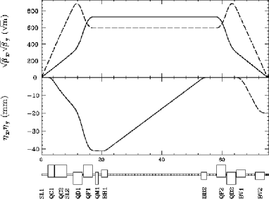
Figure 7.25: Optics of the beam extraction line.

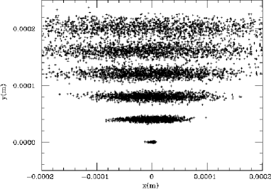
Figure 7.26: Transverse distribution of monochromatic beams at FP2.

To study beam loss, a tracking was performed using SAD, where 40000 macro particles were used. The initial conditions of the macro particles were also calculated using the CAIN. Some simple aperture at each magnet was assumed and particles went out of it was assigned to be lost at the position. Figure 7.28 shows the energy distribution of survived particles (solid) and that of lost particles (dashed). About 0.9% of the total particles (which had low energy) were lost. Figure 7.28 shows the rate of neutron dose at the interaction point. We assumed that one neutron would be created per 10 GeV beam loss. The neutron dose was calculated considering the distance between the IP and the lost position assuming no shielding between them. In total, $4\times 10^{11}/{\rm cm}^{2}$ neutron dose is expected in one year. This result may not be acceptable. But it should be noted that the self-shielding effect or additional shield is not included in this study. In addition, more realistic (and complicated) assumption of the aperture may reduce the beam loss. If we loosen the requirement for the resolution of the energy distribution measurement, the beam line optics may be modified to reduce the beam loss.

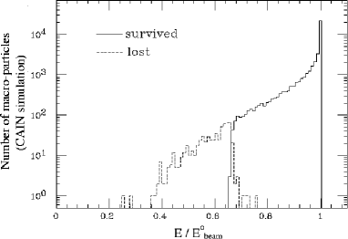
Figure 7.27: Energy distribution of survived particles (solid) and lost particles (dashed).

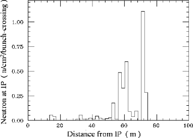
Figure 7.28: Rate of neutron dose at the interaction point ($/{\rm cm}^{2}/$bunch crossing).

Chapter 8 Tracking

8.1 Vertex Detector

8.1.1 Overview

Design Criteria

The primary role of the vertex detector is to reconstruct the secondary and tertiary decay vertices of B and D meson decays and tag bottom($b$) and charm($c$) quark jets. Distinguishing heavy flavor ($b$ and $c$) jets from light flavor($u$, $d$, and $s$) jets is relatively easy. It can be achieved by looking for tracks which have impact parameters significantly greater than zero. In precision measurements of some physics processes at the linear collider, discrimination between $b$ and $c$ quark jets is required. In this case reconstruction of secondary and tertiary vertices is necessary for efficient discrimination of $b$ jets from $c$ jets. Better spatial resolution and tracking efficiency are required for the vertex detector to obtain better tagging efficiency of the jet flavor.

The vertex detector consists of several layers of sensors surrounding the interaction point concentricaly. Vertex reconstruction is performed by extrapolating tracks measured by several layers of the sensors. In order to get better vertex resolution and better flavor tagging efficiency, the vertex detector should have the following features:

• The length of the extrapolation should be as short as possible, i.e., the innermost layer should be as close to the interaction point as possible.

• To minimize the effect of multiple scattering, the thickness (in radiation length) of the sensors and supporting ladders, particularly that of the inner most layer, should be as thin as possible.

• The sensors should be two-dimensional (pixel type) sensors with high granularity in order to separate near-by tracks in a collimated jet. Of course better spatial resolution is desirable.

When we try to satisfy these requirements, we are faced with several difficulties. As discussed in section 7.4 the track density of the pair background particles increases near the interaction point. High background hit rate causes the problems of wrong tracking due to fake hits leading to poor vertex resolution, and radiation damage of the sensors. Therefore there is a limit on the minimum radius of the inner most layer. The existence of the beam background gives rise to another requirement for the vertex detector:

• The sensors used for the vertex detector should have enough radiation immunity so that the first layer can be located in the vicinity of the interaction point.

Possible Options

The vertex detector has to consist of pixel type sensors not only for the separation of tracks in a collimated jet but also for the detection of tracks in the environment where a large number of the beam background hits exist. The following technologies can be candidates for the sensors used for the vertex detector.

• CCD: CCD (Charge Coupled Device) is an established technology widely used also in commercial products. The thickness of the sensitive region is about 20 $\mu$m. The wafer thickness can be thinned down to 20 $\mu$m provided that the mechanical strength is assured with an adequate method. Large size chips ($1.6\times 8\ \mbox{\rm{cm}}^{2}$ for SLD [1]) can be made. Relatively sensitive to radiation damage.

• CMOS pixel sensor: In CMOS pixel sensors, each pixel has a sensor diode and a read-out amplifier. Signals from the pixels are read out by x-y addressing. The thickness of the sensitive region is about 20 $\mu$m. The radiation immunity is better than that of CCDs.

• Hybrid pixel sensor: Hybrid pixel sensors have a sensor diode wafer and a readout wafer connected by bump bonding technique. This structure inevitably makes them thicker than CCDs or CMOS sensors. The radiation hardness is excellent.

Among the options listed above, we regard the CCD as a primary candidate for the sensor used for the vertex detector at JLC. We have been studying on the properties of CCD sensors extensively in order to demonstrate the feasibility for the vertex detector at the linear collider experiment. The detail will be described in subsections 8.1.2 and 8.1.3.

Detector Configuration

One possible schematic design of the CCD vertex detector, which is put in the JLC detector full simulator (JIM), is shown in Fig. 8.1. Main parameters of the detector are:

• Four layers of CCDs placed at $r=$24, 36, 48, and 60 mm.

• Each layer has an angular coverage of $|\cos\theta|<0.9$.

• The thickness of each layer is 300 $\mu$m.

• The pixel size of the CCD is 25 $\mu$m square.

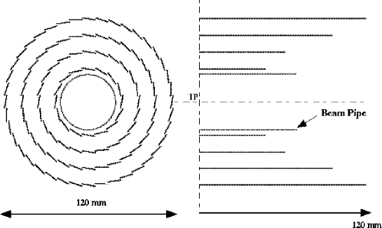
Figure 8.1: Schematic design of the CCD vertex detector for JLC.

Hit density of the vertex detector is quite high due to collimated jets and the pair-background hits. In such a situation, at least four layers are necessary for local track finding and self calibration using the vertex detector alone.

In a simple model of the vertex detector which has two layers at $r_{in}$ and $r_{out}$ with the spatial resolution of $\sigma_{in}$ and $\sigma_{out}$, respectively, the impact parameter resolution $\sigma_{b}$ can be expressed as

$$\sigma_{b}={{\sigma_{in}r_{out}}\over{r_{out}-r_{in}}}\oplus{{\sigma_{out}r_{in}}\over{r_{out}-r_{in}}}\oplus{{0.014r_{in}}\over{p\beta}}\sqrt{X_{r}\over\sin^{3}\theta},$$ (8.1)

where $X_{r}$ is the thickness of the inner layer in radiation length, $p$, $\beta$, and $\theta$ are momentum, velocity, and polar angle of the charged particle, respectively. Outer radius of the vertex detector has less importance on the impact parameter resolution as long as $r_{out}\mathchar 12829\relax r_{in}$ is satisfied. In the case of the JLC detector model, the impact parameter resolution for high momentum particles better than the expression 8.1 is achieved by combining the vertex detector and the CDC. The reason of this fact is that taking four layers of the vertex detector together as the “in” layer and the CDC as the “out” layer in the expression 8.1 gives smaller value for the first two terms in equation 8.1. Then important parameters for the vertex detector are $r_{in}$(radius of the innermost layer), $\sigma_{in}$(spatial resolution), and $X_{r}$(detector thickness).

The innermost layer of the vertex detector is conservatively located at $r=24$ mm in the present design. With this configuration, $e^{\pm}$ dose of $\sim 1.5\times 10^{11}/\mbox{cm}^{2}$ is expected in one year at the innermost layer with the solenoid magnetic field of 2 Tesla and with the accelerator parameter set of “A” described in section 1.4.2. As will be shown in subsection 8.1.3, the CCDs of the innermost layer would stand operation of more than 3 years under this rate of radiation dose. If stronger magnetic field is employed, the pair-background particles are confined in the region of smaller radius and the first layer of the vertex detector can be placed closer to the interaction point. The same background rate is expected at $r=20$ mm with $B=3$ Tesla. If still smaller radius is required, or if the luminosity of the machine is increased (the machine parameter set “Y” in section 1.4.2, for example), more frequent replacement of the damaged CCDs, still stronger magnetic field, or devices more radiation hard are required.

One of the advantages of the CCD as a tracking device is its excellent spacial resolution. Structure of a CCD sensor is schematically shown in Fig. 8.2. The epitaxial layer of $\sim 20\ \mu$m thick is the sensitive region. Since most of the epitaxial layer is not depleted, the signal charge (electrons of e/h pairs) diffuses thermally in the epitaxial layer and spreads over several pixels even for the normal incident particles. Consequently, high precision position measurement can be achieved by the charge sharing.

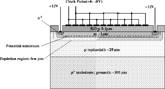
Figure 8.2: Structure of a CCD sensor.

As shown in Fig. 8.2, normal CCDs have thick insensitive substrate. When used for the vertex detector, this part should be thinned as much as possible to reduce the multiple scattering of charged particles. On the other hand, it becomes more difficult to keep thin silicon wafers flat, particularly operated at low temperature [1]. We have measured the flatness of CCDs using a laser displacement meter and an x-y scanner (Fig. 8.3). We show in Fig. 8.4 a result of the flatness measurement of a commercially available CCD which has thinned sensitive area for the purpose of the back-illumination. A sizable bowing presumably due to the temperature difference between at the fabrication process and at the room temperature can be seen. From this point of view, operation of the vertex detector at near room temperature is desirable to minimize the distortion of the CCD wafers. The mechanical structure which can keep the thin CCD wafers flat has to be studied.

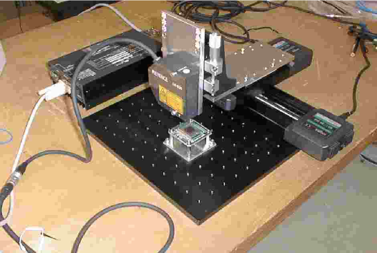
Figure 8.3: Measurement system of CCD flatness.

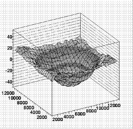
Figure 8.4: Measured surface flatness of a back-thinned CCD sensor. (units in $\mu$m)

Each CCD wafers will have multiple readout nodes so that all pixels can be read out during the train crossing interval of 6.7 msec. If we conservatively assume the readout frequency of 10 MHz, each readout channel can read out the area of about $0.4\ \mbox{\rm cm}^{2}$ between the train crossings. Since the total area of the CCDs in the vertex detector is about $2000\ \mbox{\rm cm}^{2}$, about 5000 readout channels are needed. Higher readout frequency or longer readout period by vetoing next collision(s) can reduce the number of the readout channels.

R& D Status

So far, our R&D effort has been devoted mainly to the study of the spatial resolution and the radiation hardness of CCD sensors. In the following subsections, we will describe results of the study in detail and demonstrate the feasibility of the CCD vertex detector. In particular, with the conservative design described above (machine parameter set “A” and $r_{min}=24$ mm), it will be shown that the operation of CCD vertex detector near room temperature ($\sim 0^{\circ}C$) is feasible.

8.1.2 Study of Spatial Resolution

Factors Affecting the Spatial Resolution

The most important parameter for the vertex detectors is the spatial resolution. Quite a number of factors can affect the spatial resolution. The most obvious is the pixel pitch, but other intrinsic effects can be very important. In the case of an analogue readout system, the spatial resolution of CCD detectors depends on the following parameters:

1. Signal to Noise ratio (S/N).

2. Charge sharing due to carrier diffusion.

3. Digitization resolution in readout system.

We have carried out test beam to measure the spatial resolution in CCD detector. The influence of those parameters to the spatial resolution are presented here.

Test Beam

We have tested three types of CCD detectors in Multi Pinned Phase(MPP) operation [2]. In the MPP mode, the array clocks are biased sufficiently negative to invert all phases and the surface potential is “pinned” to substrate potential. As a result, the thermal excitation of electrons is extremely suppressed. It reduces the dark current by a factor of 20 compared with normal non-inverted operation mode. Table 8.1 is a list of the test samples with important parameters. Two of the three CCDs were S5466 [3] fabricated by Hamamatsu Photonics K.K. (HPK) , but with different depth of epitaxial layers, 10$\mu$m (HPK10) and 50$\mu$m (HPK50), respectively. HPK10 is a commercially available, but HPK50 is specially fabricated for this experiment. Those consists of 512 $\times$ 512 pixels and the pixel size is 24 $\mu$m $\times$ 24 $\mu$m. Another one was CCD02-06SIS [4] fabricated by EEV Company and is also commercially available. The CCD02-06SIS consists of 385 $\times$ 578 pixels and the pixel size is 22 $\mu$m $\times$ 22 $\mu$m. It has epitaxial depth of 20$\mu$m (EEV). HPK devices are two-phase CCD, while EEV device is a three-phase CCD.

Table 8.1: Test Samples.

Test	CCD	Image	Pixel	Pixel	Epitaxial	Amplifier
sample	type	area	pitch	format	layer	sensitivity
		[mm]	[$\mu$m]	(H$\times$V)	[$\mu$m]	[$\mu$V/e]
HPK10	S5466	12.29$\times$12.29	24$\times$24	512$\times$512	10	2.0
HPK50	S5466(Special)	12.29$\times$12.29	24$\times$24	512$\times$512	50	2.0
EEV	CCD02-06	8.5$\times$12.7	22$\times$22	385$\times$578	20	1.0

A CCD tracker (Fig. 8.5) was set up at the T1 test beam line of the 12-GeV proton synchrotron (PS) at High Energy Accelerator Research Organization (KEK) as shown in Fig. 8.6.

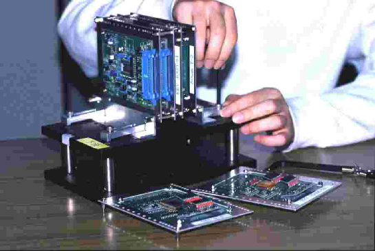
Figure 8.5: Setup of the CCD tracker.

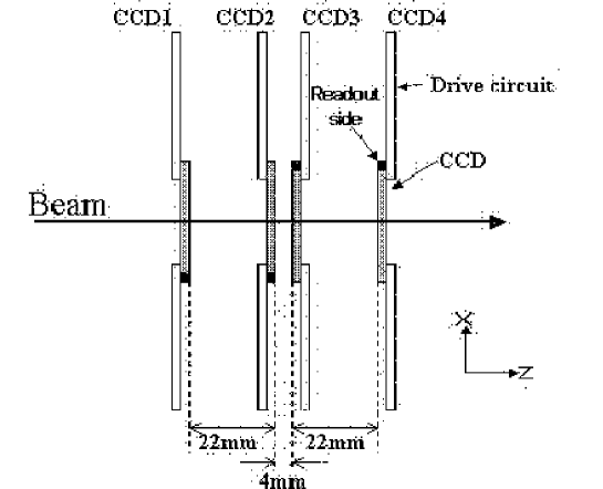
Figure 8.6: Schematic view of the setup. Both CCD1 and CCD2 were reference CCDs for tracking. CCD3 was the test sample. CCD4 was used for reduction of the accidental tracks, and the measurement of the efficiency.

The negative pion beam was used in the experiment. The momentum of the beam was chosen to be 2.0 GeV/c, 1.0 GeV/c, 0.7 GeV/c, and 0.5 GeV/c. The normal axis of the CCD tracker was aligned to the beam. The tracker consisted of four layers of CCDs as shown in the figure. First and second layers of CCDs are reference detectors for precise reconstruction of a particle track. The CCD in third layer is the sensor under test in this experiment. Another reference CCD was located at the end of the tracker for the reduction of accidental tracks. The reference CCDs were HPK/S5466 with epitaxial depth of 10$\mu$m and were same type with HPK10. All of the CCDs were driven at a rate of 250 kpixels/s, and operated in a full-frame readout mode. The CCD’s were read out every three seconds to synchronize with the PS cycle using 12-bit analog-to-digital converter(ADC). The sensitivities of the test samples including the gain of amplifier are 61.7$\pm$0.03$\mu$V/electron, 23.99$\pm$0.03$\mu$V/electron, and 34.63$\pm$0.02$\mu$V/electron, for HPK10, HPK50, and EEV, respectively. The details of this experiment are described in elsewhere [5].

Signal to Noise Ratio

The charge created by a penetrating particle is collected generally by several consecutive pixels, which form a cluster. In order to find the cluster, we first look for a leading pixel whose charge is higher than the threshold and is highest in the adjacent 6$\times$6 pixel region. The threshold was defined as 13, 7, and 15 times of the noise level, for EEV, HPK10, and HPK50, respectively, in order to reduce the noise contribution with keeping the efficiency good.

Total charge of the cluster is sum of the charges of the leading pixel and neighboring pixels. Fig.8.7 shows a typical event of a minimum ionizing particle which was detected in HPK10.

Figure 8.7: Typical event by a minimum ionizing particle detected in HPK10, where the height is a collected charge in the unit of electrons after the correction of the sensitivity of the detector including the gain of the amplifier.

Figure 8.8: Collected charge for a minimum ionizing particle as a function of clustering size, where clustering size was defined as N$\times$N pixels. The horizontal axis represents a number of N and vertical axis is a collected charge in the unit of electrons after the correction of the sensitivity of the detector including the gain of the amplifier.

Fig.8.8 shows clustering size dependence of the total charge at $-$15^∘C, where clustering size is defined as N$\times$N pixels. As shown in the figure, almost all the deposited charges are collected in the cluster size of 2$\times$2 pixels for HPK10 and EEV. For HPK50, however, more than 5$\times$5 pixels are necessary to collect all of the deposited charges. Approximately 920 electrons/10$\mu$m [6] is expected to be produced by a minimum ionizing particle in silicon, which is consistent with the observed charge by taking into account the depth of epitaxial layers.

Figure 8.9: Signal-to-Noise ratio as a function of temperature, where clustering size was chosen to be 2$\times$2 pixels. In this experiment, the CCD’s were read out every three seconds to synchronize with the PS cycle. In the JLC project, however, the read out cycle of 6.7ms is planned. It is consequence of operating faster read out cycle that the noise due to dark current is suppressed and the S/N values are expected to improve significantly.

Fig.8.9 shows the temperature dependence of S/N for 2$\times$2 pixel clustering. The S/N is defined as the most probable value of the collected signal charge distribution divided by the r.m.s. of the noise charge distribution. As temperature is raised, the S/N for HPK CCDs significantly degraded due to the increase of the dark current, while the S/N of EEV has very small temperature dependence in the range from $-15^{\circ}$C to $+15^{\circ}$C. This is because the noise caused by the dark current is not a dominant source in the total noise for EEV. The main source is considered to be an external noise which comes from the cooling system. The degradation of the S/N for HPK50 in this range was larger than that for HPK10, since the dark current for HPK50 increases more rapidly than that for HPK10 as temperature rises. In the previous paper [7], the operational condition at higher temperature was discussed with the dependence of dark current on temperature and readout drive frequency. When CCD is driven at faster rate, the noise due to dark current is suppressed. Then, the S/N values are expected to improve.

Charge Sharing and Position Determination

Since the charge sharing among adjacent pixels depends on the hit position of the particle passing through the detector, it is possible to obtain better resolution by taking into account a charge sharing characterization which is the effect of the lateral charge diffusion. The position of the cluster was determined using the 2$\times$2 pixels. In this report, we adopted two ways of determination for comparison.

• The Analog-Centroid Method

  In the Analog-Centroid-Method (AC-method)[8], the hit position is reconstructed as the charge weighted average of the 2$\times$2 pixels as

  $$x=\frac{\Sigma Q_{i}X_{i}}{\Sigma Q_{i}},$$ (8.2)

  where $Q_{i}$ and $X_{i}$ represent a charge deposit and pixel position defined at the center of i-th pixel, respectively. In this method we assume a linear relation of charge deposit to the pixel position.

• The Ratio location mapping method

  In the Ratio-Location-Mapping method(RLM-method), the relation between the position $x$ of the cluster and the charge ratio $R_{x}$ of adjacent pixel was derived from the data, where $x$ was calculated by extrapolating the track from the upstream reference CCDs and normalized by the pixel pitch. The $R_{x}$ is defined using the charge deposit of adjacent two pixels as

  $$R_{x}=\frac{Q_{x}}{Q_{max}},$$ (8.3)

  where $Q_{max}$ and $Q_{x}$ are a charge deposited in the leading pixel and in the adjacent pixel to x-direction, respectively.

  Since the particle distribution within a pixel is uniform, we can assume $dN/dx$ is constant, where $N$ is a number of incoming particles. From this assumption, we can get the relation of $x$ with $R_{x}$ as $dx/dlog(R_{x})\propto dN/dlog(R_{x})$. Taking initial conditions as $x\rightarrow 0.0$ at $log(R_{x})\rightarrow-\infty$ and $x=0.5$ at $log(R_{x})=0$, we obtain following formula,

  $$x(log(R_{x}))=\frac{0.5}{N}\int_{-\infty}^{log(R_{x})}\frac{dN}{dlog(r)}dlog(r),$$ (8.4)

  where $dN/dlog(r)$ is a $R_{x}$ distribution which is obtained from the data. The initial conditions correspond to the center of leading pixel, and the middle point of the gap between two pixels, respectively.

  Fig. 8.10(a) shows data points derived by Eq.8.4 and RLM function obtained by fitting to the data with six order polynomial function. Fig. 8.10(b) shows a linear relation which is defined as $x=0.5R_{x}$ and allowed region of the AC-method with 2$\times$2 clustering which is obtained from Monte Carlo simulation.

  

  
  

  Figure 8.10: The relation between the cluster position $x$ and the charge ratio $R_{x}$, where $x$ is the position of the cluster normalized by pixel pitch. (a)RLM function, where symbols represent measured data and lines are obtained RLM function. (b)Linear function, where boxes region shows the allowed region of the AC-method which uses 2$\times$2 pixels. Solid line represents a linear relation $x=0.5R_{x}$.

  The position of the cluster was then calculated from the measured charge ratio by using the RLM function. The RLM function represents a spread of charges produced by incident particle. For example, if a particle hits the position $x$=0.3, the charge sharing to the adjacent pixel is about 8%, 13%, and 25% of the leading pixel, for EEV, HPK10, and HPK50, respectively. HPK50 has more spread signal than HPK10, since the epitaxial depth of HPK50 is larger than that of HPK10. The charge sharing of EEV is smallest among all samples. This reason is considered that the EEV has different structure from HPK type of CCDs.

  In the AC-method, the linear relation between the position of the cluster and the charge ratio of the four pixels is assumed. However, the relation between $R_{x}$ and $x$ is not linear as shown in Fig. 8.10. Therefore, we can expect to obtain better position resolution by using the RLM-method.

Measured Spatial Resolution

The spatial resolution was derived from the residual distributions, which is the deviation of the cluster in the test sample from the extrapolated hit position from the upstream reference CCDs. The residual resolution ($\sigma_{\mbox{\rm residual}}$) was obtained by fitting this distribution with the Gaussian distribution. The $\sigma_{\mbox{\rm residual}}$ contains the contributions from multiple Coulomb scattering (MCS) and the finite resolution of the reference CCDs. The MCS effect is suppressed by the factor $(\beta cp)^{-1}$, where $\beta c$ and $p$ is a velocity and momentum of incoming particle. We derived the residual resolution at infinite momentum by fitting the momentum dependence of residual resolutions with the function $\sigma_{\mbox{\rm residual}}=\sqrt{A^{2}+(B/\beta cp)^{2}}$, where $A$ and $B$ are fitting parameters, and $A$ represents residual resolution at infinite momentum. Fig. 8.11 shows the momentum dependence of residual resolution with fit result.

Then the contribution from the ambiguity of the extrapolated hit position due to the finite resolution of the reference CCDs are estimated by taking the propagation of errors, and subtracted from the data. Here, we assumed spatial resolutions of reference CCDs were same as HPK10, because the reference CCDs were same type with HPK10.

Figure 8.11: The momentum dependence of the residual resolutions for a)AC-method and b)RLM-method. The lines are results of fit to data.

The obtained spatial resolutions for normal incidence are listed in the Table 8.2, for the AC-method and the RLM-method, respectively. At $-$15^∘C, the spatial resolutions for HPK10 and EEV were improved about 20% by taking the nonlinear charge sharing characteristics by the RLM-method into account. When the temperature was raised from $-$15^∘C to $+$5^∘C, the spatial resolutions obtained by using the RLM-method were changed its values according to the variation of the S/N value, i.e. about 20% worse for HPK10, and almost unchanged for EEV. On the other hand, the spatial resolutions derived from the AC-method were almost same, even if the temperature was changed from $-$15^∘C to $+$5^∘C. Since the charge sharing is small in adjacent pixels for HPK10 and EEV, the resolution of $R_{x}$ is deteriorated by the noise. This is the reason why the RLM-method is more sensitive to the S/N value than the AC-method. This conjecture explains the temperature dependence for HPK10 and EEV as well. For HPK50, the spatial resolutions obtained by the RLM-method and the AC-method were almost same value at both $-$15^∘C and $+$5^∘C, because the RLM function is similar to the function in the AC-method as shown in Fig. 8.10(b). The spatial resolution becomes worsened about 30% if the temperature was raised from $-$15^∘C to $+$5^∘C. This is caused by the 50% degradation of S/N ratio.

Table 8.2: Spatial resolution in $\mu$m.

Temperature	Method	HPK10	HPK50	EEV
$-15^{\circ}$C	AC	3.56$\pm$0.02	2.67$\pm$0.09	3.71$\pm$0.08
	RLM	2.76$\pm$0.03	2.79$\pm$0.09	2.94$\pm$0.10
$+5^{\circ}$C	AC	3.68$\pm$0.03	3.34$\pm$0.10	3.84$\pm$0.08
	RLM	3.46$\pm$0.04	3.67$\pm$0.12	2.59$\pm$0.16

Efficiency

Efficiency was measured by looking for the existence of associated cluster in the interpolated region on the test sample, for the tracks which have a cluster in three reference CCDs. We require that the reference CCD at the end of tracker must have a associated cluster within 5 times of alignment errors from extrapolated hit position, for the reduction of the accidental tracks. The threshold for a leading pixel were applied as 13, 7, and 15 times of the noise level, for EEV, HPK10, and HPK50, respectively. Efficiencies at $-15^{\circ}$C for 2 GeV pion were 98.8${}_{-1.5}^{+1.2}$%, 99.4${}_{-1.6}^{+0.6}$%, and 97.8${}_{-1.6}^{+2.2}$%, for HPK10, HPK50, and EEV, respectively.

Discussion

• Signal-to-Noise dependence

  The result from the test beam shows the degradation of the spatial resolution due to the increase of noise. We have estimated the influence of noise on the spatial resolution. The signals from CCDs are smeared with pseudo-noise that was generated according to the deviates drawn from a Gaussian distribution. Fig. 8.12 shows the dependence of the resolution on the 2$\times$2 clustered signal-to-noise ratio. The RLM-method is sensitive to the S/N value, but it can improve resolution if the S/N is good enough. On the other hand, the AC-method is less sensitive to the S/N value than the RLM-method. In the case of EEV, the AC-method shows that the spatial resolution is almost unchanged even if the S/N is decreased from 19 to 7. The RLM-method requires the S/N about more than 10 for EEV and HPK10, to obtain better spatial resolution than the AC-method.

• Digitization resolution dependence

  An analog readout is a preferred solution for several reasons, including more effective monitoring of the stability of the detector properties and improvement in the spatial resolution. We need to know how many bits are required for quick extraction of the digitized information and reduction of the data size. We have investigated the spatial resolution by varying the digitization accuracy. Since we have used a 12-bit linear ADC for this experiment, we varied the digitization accuracy by using only higher bit information, while the dynamic range was unchanged.

  Fig. 8.13 shows the digitization accuracy dependence of spatial resolutions, for the RLM-method and the AC-method, respectively. The spatial resolutions are almost unchanged even if the digitization accuracy is reduced to 10 bits. If the accuracy was reduced less than 10 bits, the spatial resolution become worse. Fig. 8.14 shows the considerable event pattern and its observed pattern when the ADC accuracy is reduced. The worst spatial resolution at 6 bits is explained by the “symmetry” observed pattern that is described in Fig. 8.14(c). In this case, there is the ambiguity of choice of clustering. The cluster can be one of two types of clustering, and loose direction information. Fig. 8.15 shows the mean value of output signals in units of ADC counts. The points shown in the figure are output level of horizontal over clock(HOC), dark charge which was derived with 12 bit resolution, the leading pixel in the cluster($P_{max}$), the pixel which is the adjacent pixel to x-direction inside the cluster($P_{x}$), and the pixel which is in the opposite side of the $P_{x}$($P_{opp}$). We used average of HOC output as a baseline for calculation of the signals so that the HOC also affect to the other signal levels.

  As shown in the figure, $P_{x}$ and $P_{opp}$ is almost same as dark charges for EEV and HPK10, and is disappeared as reduction of ADC resolution. Then the event type become single event.

  Both of $P_{x}$ and $P_{opp}$ are separated even at the 8 bit resolution for HPK50. However, at 6 bit resolution, both signals are recognize as identical , while those are separated from dark charge. This is the case of symmetry event type and loose the direction information.

  In the case of AC-method, the signal used for position determination is defined by sum of two pixels. The reason for distortion of the spatial resolution at 6 and 4 bit ADC accuracy for HPK50 is same as that of RLM-method. But the reason is quite different for the HPK10. The distortion of the spatial resolution at 6 bit, is due to the minus signal at the adjacent pixel. The calculated position become opposite to the correct position if the adjacent signals were minus values. While the calculated position constrains to the center of the maximum pixel in RLM-method. Fig. 8.16a) shows the correlation of the ratio for cluster side and for the opposite side of the cluster for HPK50, and Fig. 8.16b) shows the residual resolution for HPK10.

Figure 8.12: Signal to noise ratio dependence of spatial resolution for (a)EEV, (b)HPK10, and (c)HPK50, respectively. Black symbols represent the data measured at -15C^∘ and +5C^∘. Open symbols represent the simulated data by smearing the data measured at -15C^∘.

Figure 8.13: Digitization accuracy dependence of spatial resolution for (a)The RLM-method and (b)The AC-method.

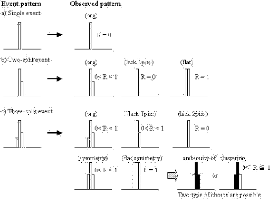
Figure 8.14: Considerable event pattern and its observed pattern.

Figure 8.15: The mean value of output signals as a function of ADC bit resolution, for the horizontal over clock(HOC) (black circle) which was used for the offset of the output, dark charge obtained with 12 bit accuracy (open circle), maximum signal in the cluster (black square), the signal used for the calculation of R (black triangle), and the signal of the pixel in the opposite direction of R (reversed black triangle). The solid and dashed lines represent 6 bit and 8 bit ADC accuracy, respectively. For the EEV, dark charge is very small, i.e 0.14 adc counts, the output of dark charge is almost same with HOC.

Figure 8.16: a) Charge ratio of the cluster side and opposite of the cluster side for HPK50 at 6 bit ADC resolution. b) The residual distribution for HPK10 at 6 bit ADC resolution, where the open area represents all tracks, and hatched area represents the tracks with minus value of the charge ratio.

Test with Laser Scanner System

The stability and excellent overall response of the detector are well known. Less widely described is the fact that the internal structure of the pixel gives rise to intra-pixel variations in response. These response modulations are particularly relevant to obtain the best spatial resolution.

We have made detail measurements of the response variations within a CCD, using a laser scanner system that gave a 2 micron resolution. Optical response of the CCD has been determined at all sample points within a pixel at wavelengths of 523 nm and 1064 nm whose absorption length is about 3 $\mu$m and 300 $\mu$m, respectively. Since the thickness of the epitaxial layer of CCDs is typically 10$\sim$50 $\mu$m, the pulsed laser of 1064 nm wavelength induces electron-hole pairs along the passage of the light nearly uniformly in the epitaxial layer of CCDs. The Laser light of 1064 nm is suitable for simulating the signal generated by charged particles in a CCD.

Fig. 8.17 shows the schematic view of the experimental arrangement. The system consists of YAG laser, optics, xyz moving stage, and temperature box. A CCD is set on the xyz moving stage that can move with an accuracy of about 1$\mu$m. The CCD and xyz moving stage are in the temperature box, and kept at 0^∘C. The laser power is adjusted to simulate a pulse height of minimum ionizing particles by using ND filter. The spot size of laser light is about 2$\mu$m$\times$2$\mu$m on the surface of a CCD. Fig. 8.18 shows the result of the measurement fro EEV. The charge ratio was calculated as signal charge in a pixel normalized by total charge of the cluster, where cluster was defined by adjacent three pixels. The result of 532 nm shows rather narrow charge sharing region, because of the short absorption length which makes the effect of the lateral charge diffusion small. We observed a broad charge sharing region with a triangle shape for 1064 nm. Also there is some different property in horizontal and vertical scanning. These results are used to investigate a charge sharing property and obtain a precise RLM-function. Also, this laser scanner system will be used for the calibration of the CCDs.

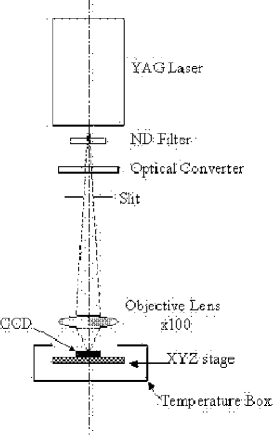
Figure 8.17: The schematic view of the laser scanner system.

Figure 8.18: The charge sharing ratio for EEV. (a) and (b) show the charge ratio in the horizontal scanning with the wavelength of 532 nm and 1064 nm, respectively. (c) and (d) show same figures in the vertical scanning. The three sets of symbols are observed charge ratio on three adjacent pixels.

Summary

We have studied the spatial resolution of a CCD. Three types of CCD detectors which have different structures were tested.

The present series of test showed that:

1)

S/N ratio of more than 10 can be achieved even at $+5^{\circ}$C and at accumulation time of 3 s including readout time, by successful operation in the MPP mode. In the JLC project, the readout cycle is much faster than this experiment. We expect the S/N become better, because noise due to the dark current is largely suppressed.

2)

The spatial resolutions were improved for HPK10 and EEV by taking the nonlinear charge sharing characteristics into account by the RLM-method.

3)

The temperature dependence of the spatial resolution in the AC-method was small for HPK10 and EEV samples, while spatial resolution become worse about 30% if the temperature was changed from $-15^{\circ}$C to $+5^{\circ}$C for HPK50.

4)

The RLM-method needs S/N more than 10 for EEV and HPK10 to keep the spatial resolution better than the AC-method.

5)

More than 10 bits digitization accuracy is needed to keep the spatial resolution better.

6)

The precise measurement of the charge sharing property was studied using laser scanner system. This system will make it easier to measure CCD property.

8.1.3 Radiation Hardness of CCD Sensors

The backgrounds at the future LC pose significant challenges to the radiation hardness of CCD sensors. The main component of the background comes from $e^{+}e^{-}$ pairs with estimated 10-year fluence of $\approx 1.5\times 10^{12}$ cm^-2. Neutron background from ($\gamma$, $n$) reactions is also present, reaching $\approx 5\times 10^{9}$ cm^-2 for the same period. The electron background is expected to affect mainly the CCDs in the innermost layer, because it is closest to the beam pipe. The neutron irradiation is almost uniformly distributed in the volume of the vertex detector and affects all CCD chips.

Study of commercially available CCDs is required to build a model for the radiation damage effects, which can be used for estimation of the device lifetime in the expected environment. Radiation hardness studies of CCDs can provide valuable information on the preferable device architecture, chip geometry and operating conditions, which ultimately determine the vertex detector design, performance and cost. Much of this study was concentrated on the device application at near-room temperature because of the advantages of this operation. Operation at low temperatures is usually required to suppress the radiation damage effects in CCDs [9]. By avoiding cooling to cryogenic temperatures it is possible to decrease the thermal distortions of the supporting CCD ladders and to simplify their design, which results in better detector geometry and increased measurement precision. Although attractive from designer’s point of view, operation at elevated temperatures faces problems from radiation damage effects, which are addressed in this study.

Both surface and bulk damage effects are expected to take place in the CCD sensors because of the type and the energy spectrum of the radiation background. Ionizing radiation creates electron-hole pairs in silicon dioxide, which is used as gate and field dielectric in CCDs. Charge carriers drift in the electric field (externally applied or built-in) to the corresponding electrode. Electrons quickly reach the positive electrode, but some of the holes remain trapped in the oxide and give rise to radiation-induced trapped positive oxide charge, which can be stable for long time. At any Si-SiO₂ interface there are a number of interface traps, which result from the strained or dangling silicon bonds at the boundary between the two materials. Ionizing radiation causes the density of these traps to increase, generating radiation-induced interface traps. The formation of radiation-induced trapped oxide charge (or flat band voltage shift) and interface traps is referred under the term surface damage.

Radiation with sufficiently high energy can displace Si atoms from their lattice positions, creating displacement damage. This process affects the properties of the bulk semiconductor and is known as bulk damage. Low energy electrons and X-rays can deliver only small energy to the recoil Si atom and mainly isolated displacements, or point defects, can be created. On the other hand, heavier particles, such as protons and neutrons can knock out silicon atoms which have sufficient energy to displace other atoms in the crystal. The secondary displacements form defect clusters, which have high local defect density and can be tens of nanometers wide. Defect clusters often have complicated behavior and more damaging effect on the properties of semiconductor devices than point defects. The energy threshold for displacement of a Si atom has been estimated to be about 260 keV for electrons and 190 eV for neutrons, therefore in the expected radiation environment bulk defects can be generated by both particles. Cluster damage is also expected, because the threshold for cluster production is known to be $\approx$5 MeV and $\approx$15 keV for electrons and neutrons [10], respectively.

Trapped holes in the oxides change the parameters of MOS structures in a way identical to applying an external voltage to the gates. Small flat band voltage shifts, in the order of few volts, can be accommodated by adjustment of the amplitude of the gate bias and drive voltages. A limitation may arise from the maximum allowed power dissipation in the gate drivers and in the CCD chip, because the dissipated power is proportional to the voltage amplitude squared. If the flat band voltage shifts are higher, the device can stop to function properly because of parasitic charge injection from the input structures, incomplete reset of the output node or distortion of the shape of the potential wells [11]. However, as long as no parasitic effects from the increased pulse amplitudes appear, the shifts are not a limitation for the device operation.

Interface traps are the dominant source of dark current in modern CCDs, because the generation rate at the Si-SiO₂ interface is usually higher than that in the epitaxial bulk silicon. Increase of the surface dark current is the main effect expected from radiation-induced interface defects.

Radiation-induced bulk defects cause the dark current in CCDs to increase, which is well known phenomenon [12] [13]. Dark current is an issue only for near-room temperature operation or long integration times, because it can be reduced to negligible values by cooling. Irradiation with heavy particles (e.g. protons, neutrons) often creates large non-uniformities in the dark current spatial distribution in the CCDs [14]. These non-uniformities, also known as “dark current spikes” or “hot pixels” manifest themselves as pixels with much higher dark current than the average value for the CCD. Their presence has been connected with the high electric fields caused by the device architecture and field-enhanced emission, the cluster nature of the radiation damage and crystal strains in the silicon material. Dark current spikes have big consequences for high temperature applications. Additionally, some of them show random fluctuations of the generated current, or Random Telegraph Signals (RTS) [15].

Another important bulk damage effect is the loss of signal charge during transfer, or Charge-Transfer Inefficiency (CTI). Charge losses occur when bulk defects capture electrons and emit them at a later moment, so that the released charge cannot join the original signal packet from which it has been trapped. The basic mechanism can be explained by the different time constants and temperature dependencies of the electron capture and emission processes. In the presence of bulk defects electrons are trapped with a capture time constant of $\tau_{c}$ and consequently released with an emission time constant of $\tau_{e}$. For a defect at energy position E_t below the conduction band the Shockley-Read-Hall theory gives

$$\tau_{e}=\frac{1}{\sigma_{n}X_{n}v_{th}N_{c}}\mbox{exp}\ \left(\frac{E_{t}}{kT}\right)$$ (8.5)

and

$$\tau_{c}=\frac{1}{\sigma_{n}v_{th}n_{s}},$$ (8.6)

where

$\sigma_{n}$	=	electron capture cross section,
$X_{n}$	=	entropy change factor by electron emission,
$v_{th}$	=	thermal velocity for electrons,
$N_{c}$	=	density of states in the conduction band,
$k$	=	Boltzmann’s constant,
$T$	=	absolute temperature,
$n_{s}$	=	density of signal charge.

The capture time constant is typically of the order of several hundred nanoseconds and has weak temperature dependence, whereas the emission time constant changes many orders of magnitude because of the exponential temperature behavior. At low temperature the defects can be considered almost permanently occupied with electrons, because the emission time constant of the defects can be very large, of the order of seconds. The defects cannot capture signal electrons and the CTI at low temperature is small. At high temperature the emission time constant becomes small and comparable with the charge shift time. Trapped electrons are able to join their signal packet, because most of them are emitted already during the charge shift time, and charge losses are small. At temperatures between the two extremes these is a peak of the CTI value.

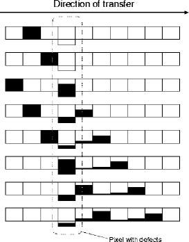
Figure 8.19: Schematic representation of the mechanism of charge transfer losses. For simplicity it has been assumed, that only one pixel contains defects.

The mechanism of charge transfer losses is illustrated on Fig. 8.19. When the signal packet encounters traps, some of its electrons are captured and later released. Those electrons, which are released in the trailing pixels do not join their original signal packet and account for the CTI. If a charge packet enters a pixel, in which part of the traps are occupied, less signal electrons can be trapped and therefore less charge can be lost.

We are often interested not only in the CTI value, but in the total losses the charge suffers after all the transfers it takes to reach the output. For a generated charge $C_{gen}$, transferred $n$ times, the output charge $C_{out}$ is given by

$$C_{out}=C_{gen}(1-CTI)^{n}.$$ (8.7)

This dependence shows, that CTI and the number of transfers are the two important parameters that need to be considered for minimizing the charge transfer losses.

Dark Current and Flat-Band Voltage Shift

For near-room temperature applications one is particularly concerned with the dark current of the CCD sensors. Multi Pinned Phase (MPP) mode CCDs [16] were used in our experiments because they feature much lower dark current than standard devices. In MPP CCDs the Si-SiO₂ interface is biased into inversion and populated with holes, leading to suppression of the carrier generation from interface defects. With the surface inverted, only bulk defects contribute to the dark current. Since in contemporary buried channel CCDs current generation from defects at the Si-SiO₂ interface is dominant, MPP mode operation can reduce the device dark current by more than one order of magnitude. This method has the ability to suppress the dark current from the interface states formed during irradiation and can offer increased radiation hardness [17].

The radiation hardness of two types of buried channel, MPP mode CCDs was studied. The S5466 CCD, manufactured by Hamamatsu Photonics is 2-phase device with 10$\mu$m epitaxial layer and 512$\times$512 active pixels with size 24$\mu$m$\times$24$\mu$m. Three other types of S5466-based CCDs were studied, including high speed device (10 Mpix/s), notch CCD and device with SiO₂-Si₃N₄-SiO₂ gate (ONO) dielectric. A three-phase CCD, manufactured by EEV Ltd. was investigated as well. The device CCD02-06 has 20$\mu$m epitaxial layer and 385$\times$578 active pixels with size 22$\mu$m$\times$22$\mu$m.

Several devices were exposed to electron irradiation from a ⁹⁰Sr source and 2 CCDs were irradiated by neutrons from a ²⁵²Cf source. The change of the voltage needed to achieve MPP mode operation was used as a measure of the flat band voltage shifts. The dark current of the devices was measured in the temperature range from $-100^{\circ}$C to $+20^{\circ}$C by averaging the dark charge over several frames. The CTI of the horizontal (serial) and the vertical (parallel) registers of the CCD was measured in the same temperature range by observing the charge and the position of isolated pixel events (IPE), created by the 5.9 keV Mn-K_α line of a ⁵⁵Fe source. After sufficient averaging, the dark signal of each pixel was stored into memory and this dark frame was then subtracted pixel by pixel during the X-ray exposure. The readout speed was usually 250 kpixels/s. For the high-speed Hamamatsu CCD the speed was raised to 2 Mpixels/s.

The change of the MPP threshold voltage in electron-irradiated S5466 CCD, irradiated unbiased, is shown in Fig. 8.21. Due to the SiO₂-Si₃N₄ gate dielectric in the EEV devices, the change of the MPP threshold is slightly smaller than than in Hamamatsu CCDs. In biased and clocked S5466 CCD higher shift was observed (Fig.8.21), which is explained by the lower ratio of recombining holes in biased oxides. The flat band voltage shifts were estimated to be 0.02 V/krad for unbiased devices and 0.07 V/krad for biased Hamamatsu CCDs. The flat band voltage shift of electron-irradiated Hamamatsu ONO CCD was also measured, however it was higher that in standard S5466 devices, on the contrary to the expectations. In neutron-irradiated devices such shifts were not expected and were not observed.

Figure 8.20: Average dark current density as a function of the electron irradiation fluence and of the negative drive pulse voltage V${}_{ee}^{V}$ at T = $-26^{\circ}$C. The device #JS14/026 is irradiated unbiased.

Figure 8.21: Average dark current density as a function of the electron irradiation fluence and of the negative drive pulse voltage V${}_{ee}^{V}$ at T = $-26^{\circ}$C. The device #JS8/053 was biased and clocked during irradiation.

The dark current in MPP mode in both electron and neutron irradiated devices increased after irradiation, which is attributed to creation of bulk traps. The CCD demonstrates effective suppression of the surface component of the dark current by almost 3 orders of magnitude (Figs. 8.21 and 8.21) when $\mid$V${}_{ee}^{V}\mid>\mid$V${}_{ee}^{MPP}\mid$ and the interface is populated with holes. In that condition the dark current is limited by carrier generation in the bulk.

Spurious dark charge, which was superimposed on the bulk current, was observed in electron irradiated Hamamatsu CCDs. This spurious current, which was named “dark current pedestal” (DCP) does not depend on the accumulation time of the readout cycle [18]. Because it is produced by the clocking, dark current measurements are not affected. However, the DCP provides background charge in the CCD and decreases the measured CTI through the “fat zero” effect. It was found, that the spurious current was caused by impact ionization by holes, returning to the channel stops and to the adjacent gates after the surface potential has been switched from inversion to depletion [19]. The temperature dependence of the DCP is shown on Fig. 8.23. In the low temperature region holes are provided by tunneling from near-interface traps, while at higher temperatures carriers are released by thermal excitation from interface defects. The DCP severely limits the application of Hamamatsu devices because it is much larger than the bulk dark current at the same temperature.

Figure 8.22: Temperature dependence of the average DCP density in device #JS14/026 as a function of the electron irradiation. Dashed line shows the calculated temperature dependence of the hole ionization rate at $10^{5}$ V/cm.

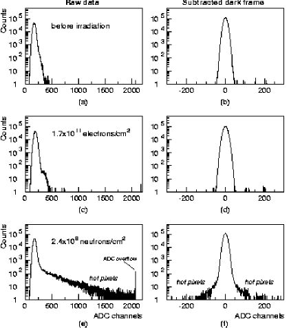
Figure 8.23: Dark current distribution at +10^∘C in S5466 CCDs before irradiation (a), (b); in an electron irradiated to $1.7\times 10^{11}$ cm^-2 CCD (c), (d); and in a neutron irradiated to $2.4\times 10^{8}$ cm^-2 CCD (e), (f). The gain is $\approx$ 6.0 electrons/ADC channel.

Investigation of dark current spikes was performed on both Hamamatsu and EEV devices, which showed very similar results. No increase of the dark current non-uniformities was observed in electron irradiated devices (Fig. 8.23(a)–8.23(d)). Neutron irradiated CCDs however, showed significant creation of dark current spikes (Fig. 8.23(e)) after irradiation with fluence as low as $2.4\times 10^{8}$ neutrons/cm². After subtraction of the dark frame pixel by pixel, the resulting distribution (Fig. 8.23(f)) is close to that of a electron-irradiated CCD. This subtraction shows an efficient way to correct for the large dark current non-uniformities in CCDs, irradiated by heavy particles. During operation, the dark current map should be updated regularly to include the contribution of the newly created defects.

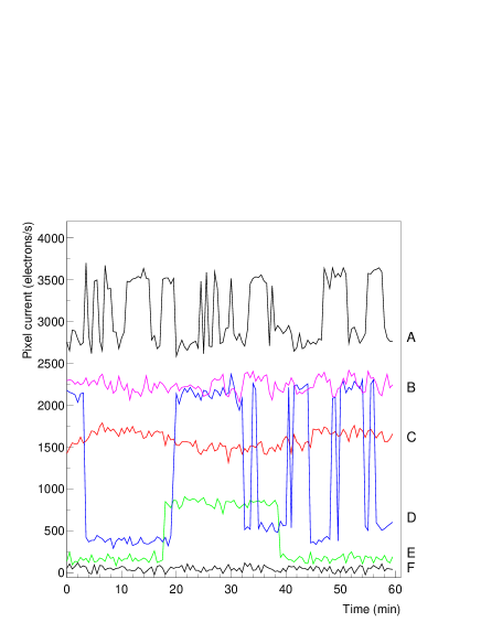
Figure 8.24: Time variation of the dark current at $-1.6^{\circ}$C in hot pixels, showing RTS behavior. The measurement was carried out on Notch CCD #P4 1-5B1-4, irradiated to $5.7\times 10^{9}$ neutrons/cm². Pixel F is normal (not “hot”), is plotted for reference.

Figure 8.25: Ratio of false IPE per CCD frame, caused by RTS, at 4 different integration times $t_{i}$. The measurement was performed on Notch CCD #P4 1-5B1-4, irradiated to $5.7\times 10^{9}$ neutrons/cm². The threshold is set at 600 electrons.

Random telegraph signals (RTS) were observed in many hot pixels when their current was recorded for sufficiently long time (Fig. 8.25). During the typical time, required for one CTI measurement ($\approx$ 5 min), these fluctuations are difficult to notice and they have small effect on the subtraction of the dark frame. In a long time scale, it is not possible to correct for the dark current of such pixels as was shown on Fig. 8.23 because of the random fluctuations of the pixel current. The RTS can generate false signals, similar to those created by X-rays or MIPs, and can be a source of erroneous track reconstruction. A measurement to find isolated pixel events, caused by RTS was performed on Hamamatsu and EEV CCDs, with similar results. The number of false IPE greatly depends on the threshold, which is imposed for the search of signal. The same threshold of 600 electrons, used for the CTI measurements was employed in the measurement. The ratio of false IPE per CCD readout frame (i.e. the pixel occupancy), caused by RTS is shown in Fig. 8.25. The RTS amplitude depends on the temperature and the integration time $t_{i}$ and these two parameters were varied during the measurement. Although about 40% of the hot pixels exhibit RTS, most of them are rejected by the applied threshold for IPE search. When the integration time is short, a ratio of false IPE signals of less than $10^{-4}$ can be achieved even in the temperature range above 0^∘C.

CTI

Much attention was paid to the measurement of radiation-induced CTI, because it is the main factor that requires low temperature operation [9]. A model for the charge transfer in 2- and 3-phase CCDs was developed [19], which allows one to calculate the CTI as a function of the temperature, timing of the transfer, concentration of background charges, signal size and pixel occupancy.

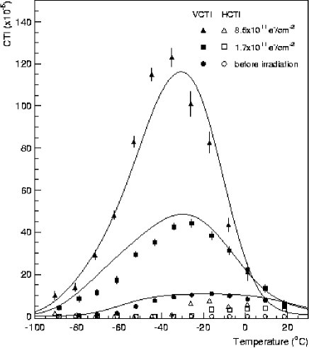
Figure 8.26: CTI as a function of the temperature and of the electron irradiation fluence in S5466 CCD. Symbols are the experimental data; solid lines represent the modeled VCTI for the combination of two traps at E${}_{c}-$0.37 eV and E${}_{c}-$0.44 eV.

Figure 8.27: CTI of 2-phase (Hamamatsu S5466) and 3-phase (EEV CCD02-06) electron-irradiated CCDs.

The results from the CTI measurements on electron irradiated S5466 CCD, together with modeled results are shown in Fig. 8.27. Modeling was performed using the experimental values of the dark current and of the DCP, presented in the previous paragraphs. The modeling on electron irradiated CCDs showed that a trap at E${}_{c}-$0.37 eV with $\sigma_{n}$ = 4$\times 10^{-15}$ cm² is responsible for the observed increase of the vertical CTI. Additional pre-irradiation defect was identified at E${}_{c}-$0.44 eV. The energy position of the main defect, derived from the model, varies between E${}_{c}-$0.37 eV and E${}_{c}-$0.39 eV in three samples. The simulated results in Fig. 8.27 are based on the presence of two traps at E${}_{c}-$0.37 eV and E${}_{c}-$0.44 eV. The concentration of the trap at E${}_{c}-$0.44 eV, obtained from the model increases insignificantly under irradiation. The CTI of the horizontal register is less than 10^-4 in the whole temperature range. As explained by the model, the peak in the HCTI, which would have occurred at high temperatures is suppressed by the dark current pedestal and the exponentially increasing dark current.

Similar result was obtained in electron-irradiated EEV CCD, however the VCTI in that device was about 4 times higher than in S5466 devices. Numerical simulations showed, that under equal conditions the 3-phase CCDs has about 2.5 times larger CTI than 2-phase devices, because of the higher signal density in 2-phase CCDs. The greater than expected difference can be explained mostly by the DCP in Hamamatsu devices, which decreases the measured CTI values by the “fat zero effect” [18]. Two-phase devices are superior to 3-phase CCDs in term of CTI and should be preferred for applications in radiation environment.

The VCTI of neutron-irradiated to 8.9$\times$10⁹ cm^-2 S5466 CCD is about 4$\times 10^{-4}$, and VCTI peak of 3$\times 10^{-4}$ was measured in an EEV CCD, irradiated with approximately the same fluence. The same defect at E${}_{c}-$0.37 eV, derived from the model, was found responsible for the CTI increase in neutron-irradiated devices. In all CCDs the HCTI is significantly smaller than the VCTI, which is explained by the different timing of the transfer in the registers.

The defect at E${}_{c}-$0.37 eV was identified from annealing studies and additional measurements as contribution from both $E$ and $V-V^{-}$ centers [19]. The $E$ center, which anneals out at $150^{\circ}$C was found to be dominant, contributing to $\approx$ 60% of the CTI peak. The measured energy position of the defects is reduced by the Frenkel-Pool effect. This effect is also responsible for the thermal activation of the dark current in most of the hot pixels.

Modeling showed, that in the accumulated 10-year background from e⁺e^- pairs of 1.5$\times$10¹² cm^-2 the VCTI will reach $1.5\times 10^{-1}$ in 3-phase EEV-like CCD. Safe margin is included in this calculation by considering the bulk damage from e⁺e^- pairs to be 10 times larger than that from ⁹⁰Sr electrons. Neutron-induced CTI is much smaller than those generated by electrons, and only the latter is being considered. Such a high CTI value is unacceptable, because the charge will be lost only after a few transfers. Measures have to be taken to decrease the VCTI, including better CCD design and appropriate device operating conditions, in order to extend the lifetime of the CCDs.

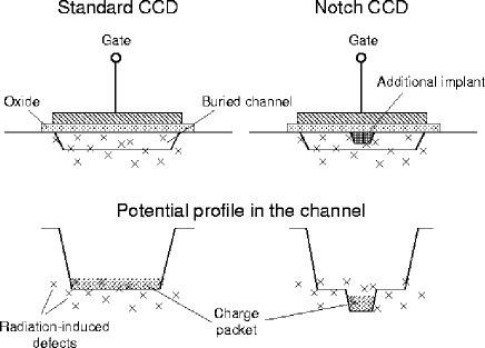
Figure 8.28: Schematic and potential profile in the channel of standard and notch CCD.

Figure 8.29: CTI of notch and standard S5466 CCDs.

One important method to improve the CTI is to use an additional narrow implant in the CCD channel (Fig. 8.29). This implant forms a sub-channel, or “notch” in the potential profile of the transport channel, confining the signal charge into a fraction of the pixel volume. CTI depends on the concentration of signal electrons $n_{s}$ as

$$CTI\propto n_{t}/n_{s},$$ (8.8)

where $n_{t}$ is the defect concentration, therefore increasing the signal density by forcing the same charge into a smaller volume can improve the CTI.

The radiation-induced CTI was measured in electron- and neutron-irradiated notch CCD, based on the S5466 design. Due to the additional 3$\mu$m-wide notch channel, its CTI is about 3 times lower than that in conventional S5466 device (Fig. 8.29). In neutron-irradiated to 5.7$\times$10⁹ cm^-2 notch CCD the peak CTI was below $10^{-4}$.

A calculation of the frequency dependence of the CTI was carried out to study the possible improvement by varying the readout speed of the CCDs. At speeds higher than several Mpix/s, horizontal CTI decreases rapidly because charge dwell time becomes shorter than the capture time constant of the defects. Vertical CTI is much less influenced, because charge spends longer time in the imaging section. Increasing the readout speed has relatively small ability to control the the VCTI and other methods to reduce it should be chosen. At high readout speed the horizontal CTI becomes more than an order of magnitude smaller than the VCTI.

It was not possible to back this calculation by experimental data from the high-speed Hamamatsu CCD, because of the dependence of the DCP on the width of the shift pulses [19]. The frequency dependence of the CTI was masked by the “fat zero” effect from the DCP and a definite conclusion could not be drawn.

Figure 8.30: Principle of thermal “fat zero” generation in MPP mode CCDs.

Figure 8.31: Measurement of CTI reduction by “fat zero” effect in EEV CCD02-06.

One of the most powerful methods, that can be used for CTI improvement is injection of a sacrificial charge, or “fat zero” into the CCD registers. This charge reduces the CTI in two ways: by increasing the signal charge density (8.8), as it is transported together with the signal; and most importantly, by filling the traps in front of the signal packet, so that less electrons can be captured.

Experimental and theoretical studies of several devices have shown, that the CTI of the vertical register dominates the charge losses in the CCD. Introducing additional charge in the vertical register through the injection port is not a trivial task because of the large non-uniformity of the injected charge [20]. We have developed another method to inject “fat zero”, which employs the dark current characteristics of MPP mode CCDs. By varying the negative gate bias voltage of the vertical register V_ee, the CCD can be driven into semi-MPP mode and its dark current can be controlled between the MPP mode value and $\approx$100 times that value (Fig. 8.31). At high temperatures, this current can be sufficient to provide charge of the order of 1000 electrons even if the CCD readout cycle is very short. The proposed method works on any type of MPP CCD, because the “fat zero” is generated thermally. The amount of injected charge can be controlled either by adjusting the V_ee, or by setting V_ee to some low value and adjusting the time, during which the CCD is out of MPP mode. Practical implementation of the proposed method depends on the irradiation level and requires precise adjustment.

Another important feature of this method is that it has the ability to self-adjust for non-uniformities of surface damage. If in some pixels the flat band voltage shift is higher, corresponding to higher surface and bulk damage, the interface component of the dark current will be higher than for the rest of the CCDs at the same setting of V_ee. Therefore, larger dark current is generated automatically, which compensates for the higher CTI in those pixels.

The experimental data in Fig. 8.31 is obtained by changing the V_ee voltage. It shows, that the CTI can be reduced several times by injecting “fat zero” of approximately 1000 electrons, which is almost half the number of signal electrons. The additional charge increases the noise of the device, however this does not degrade the performance of the high-speed CCDs, for which the readout noise is of the order of 100e^- RMS. Estimations of the radiation-induced dark current after receiving combined electron and neutron irradiation at the expected 10-year levels show that dark current generation of $>1000$ electrons can be achieved by this method at temperatures $>5^{\circ}$C and integration time of 6.7 ms.

As shown in the previous paragraphs, the VCTI is the main point of concern, because the HCTI can be reduced to less than 10% of VCTI. Using all the options for CTI improvement described above, the VCTI can be reduced more than 60 times, as shown in Table 8.3. However, this may not be sufficient, and the number of transfers in the vertical direction (i.e., the vertical chip size) may have to be reduced in accordance with (8.7) to limit the charge losses.

Table 8.3: Vertical CTI improvements.

Option	VCTI improvement
Raise the output speed to $>$5 Mpix/s	$\approx$1.3 times
Use 2-phase CCD	$\approx$2.5 times
Use notch CCD	3 to 4 times
Inject “fat zero” $>$1000 e-	6 to 8 times
Total improvement	$\approx$ 60 to 100 times

Speaking only of the CTI, the CCD lifetime in a radiation environment depends on the chosen value of charge transfer losses. Some example parameters of the CCD can be calculated if 25% lost charge is considered acceptable and the HCTI is taken as 10% of the VCTI. As was mentioned before, the VCTI of a 3-phase EEV-like CCD is expected to reach $1.5\times 10^{-1}$ after 10 years of operation in the radiation environment of the future linear collider. A CCD, which contains 2 Mpixels and 12 outputs, each reading 250 vertical and 667 horizontal pixels, will have 23% transfer losses after $\approx$3 years of operation. Although all the measures from Table 8.3 with improvement of 60 are applied in this calculation, the main contribution (18%) comes from the VCTI. Assuming pixel size of 24$\mu$m, the chip has dimensions 96mm$\times$12mm, and can be read out completely between two pulses (6.7 ms) at 25 Mpix/s.

Figure 8.32: Temperature dependence of the CTI in electron-irradiated to $8.5\times 10^{11}$ cm^-2 EEV CCD02-06 (#A4003-18) before and after annealing at $150^{\circ}$C for 2 hours.

Another possible method for reduction of the radiation-induced CTI is device annealing. It is known, that the $P-V$ center, which is the dominant bulk defect in $n$-type buried channel CCDs [15] anneals at about 150^∘C. By periodically heating of the CCD it is possible to restore the pre-irradiation CTI, provided that the mechanical support and mounting are designed to withstand such a temperature cycle.

An annealing experiment was performed on both electron irradiated Hamamatsu and EEV devices [21]. In the EEV chip the CTI decreased almost to its pre-irradiation level after 2 hours at 150^∘C (Fig. 8.32). Similar experiment on a Hamamatsu device showed CTI improvement of about 60%.

Conclusions

The most important results from the radiation damage studies of CCDs can be summarized as follows:

• The radiation hardness of 2- and 3-phase MPP mode CCDs from different manufacturers has been extensively studied;

• A model for the charge transfer losses in the CCDs has been developed and applied in good agreement with the experimental data;

• Two-phase, notch CCDs should be used because of the greatly reduced CTI in comparison to 3-phase and standard devices;

• Thermal charge injection is the major factor for reducing the CTI and promises successful near-room temperature operation in harsh radiation environment;

• Device annealing can be used for restoring the CTI to sufficiently low levels. It can be performed periodically when the detector is not working;

• Large flat band voltage shifts and spurious dark charge in Hamamatsu CCDs are the main limitations at the moment. These issuies can be solved by more advanced radiation-hard devices, currently under development.

8.2 Intermediate Tracker

The distance between the last layer of VTX and the first layer of CDC is about 39cm. The gap is filled by an Intermediate Tracker(IT). The intermediate tracker consists of five layers of silicon detectors placed at radii of 9.0, 16.0, 23.0, 30.0, and 37.0 cm and covers $|\cos\theta|<0.90$, which coincides with the region covered by VTX. The material thickness of each layer is 0.6% radiation lengths, and the spatial resolution is 40$\mu$m each for $r\phi$ and $z$.

The roles of the intermediate tracker are to improve

• the linking efficiency of a CDC track to the corresponding VTX track,

• the reconstruction efficiency of particles which decay between VTX and CDC,

• the reconstruction efficiency of low momentum tracks, and

• time stamping capability to discriminate background tracks created by off-timing bunches, which is impossible with the CCD vertex detector, since it does not provide signal timing information.

To study the efficiency to link a CDC track to the corresponding IT and VTX hits, we generated single $\pi^{+}$ events at $\cos\theta=0$ and studied the residuals of the CDC tracks at the last layer of IT (at $r=37$ cm) and the last layer of VTX (at $r=6$ cm), as shown in Fig. 8.33. Since the residuals at IT are considerably smaller than those at VTX, IT will help in extrapolating CDC tracks to the VTX region.

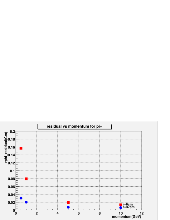
Figure 8.33: The r$\phi$ residual at the last layer of IT(r=37cm) and that of VTX(r=6cm) for pion momenta: 0.5, 1.0, 5.0, and 10.0 GeV.

We also studied residuals of tracks in Higgs events.

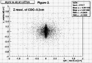
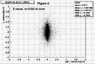
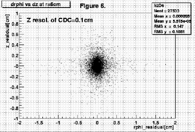
Figure 8.34: The residuals of CDC tracks at IT(r=37cm) and VTX(r=6cm) positions, for Higgs events. Upper two figures are for the case where the $Z$ resolution of CDC is 3mm, while the bottom two figures are for 1mm.

The scatter plots of residuals in the r$\phi$ plane against those in the $z$ direction are shown in Fig. 8.34. The residuals for a CDC $z$-resolution of 0.1cm is also shown for comparison. Again, we see the reduction of residuals at IT compared to those at VTX. The $z$-residual at IT is mainly due to the $z$-resolution of CDC. It is thus desirable to reduce it to 1mm or less. There are tails in the distribution at IT. They are caused by multiple scattering of low momentum tracks. By Gaussian-fitting to the central part of the distribution, we obtained the standard deviations of the residuals as summarized in Table 8.4.

Table 8.4: Summary of residuals of Higgs events at IT and VTX position.

Position	$\sigma_{z}$(mm)	$\sigma_{r\phi}$ (mm)	$\sigma_{Z}$ (mm)
IT	3	0.021	0.137
	1	0.023	0.055
VTX	3	0.039	0.187
	1	0.038	0.073

The distance ($d$) among hits in Higgs events is plotted in Fig. 8.35, at the outer-most VTX layer (r=6cm) and IT (r=37cm). The events were generated at $\sqrt{s}=300$ GeV with a Higgs mass of 120 GeV. As seen in the figure, the numbers of hits near $d$=0 increase linearly with $d$, which indicates that the hit density is uniform locally. From these figures we conclude that the density of hits at the IT position ($r=37$cm) is about 0.11 hits/mm², while that at the VTX position ($r=$6cm) is 0.66 hits/mm². In the case of $q\bar{q}$ events at $\sqrt{s}$=500 GeV, those are 0.06 hits/mm² at IT and 0.34 hits/mm² at VTX. If hit densities are high, it is difficult to associate hits with tracks extrapolated from CDC. Residuals shown in Table 8.4 represent well that extrapolated CDC tracks can resolve hits in IT or VTX. Assuming three times the residual value for the size of the window for unique hit-to-track association, the average number of false hits in that window can be obtained using the hit density. Those are 0.035(0.016) hits at IT and 0.54(0.21) at VTX when $\sigma_{z}$ of CDC is 3mm(1mm) in the case of Higgs events. Improvement of hit-track linking is clear when IT is installed.

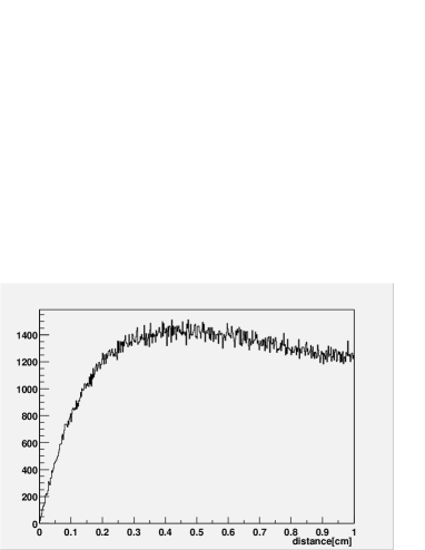
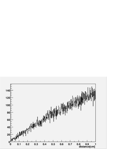
Figure 8.35: The distance among hits of Higgs events at (a) VTX position(r=6cm) and (b) IT position(r=37cm).

8.3 Central Tracker

8.3.1 Overview of CDC

We start our discussion with general design principle of a central tracker in order to translate the physics requirements to concrete chamber parameters. A possible set of chamber parameters for the central tracker is given according to the general design principle. We then list up our R&D items that include mechanical and operational stability issues, feasibility studies of required chamber performance, and effects of space charge and magnetic field. Finally we summarize our R&D and discuss future direction.

8.3.2 Design principle

Outline of Geometrical Parameters Decision Process

The parameters that determine the geometrical configuration of a small-jet-cell cylindrical drift chamber can be classified into two groups: (1) global parameters that specify the size and layout of axial and stereo super-layers, and (2) local parameters that describe the geometry of a jet cell in each super-layer. The first class includes the length, the inner and outer radii, and the stereo angle of each super-layer. If there is a layer of shielding wires between adjacent super-layers, its radius and stereo angle also belong to this class. The parameters in the second class are, essentially, the relative locations of wires that comprise a single jet cell, and determine the local properties of the chamber. These parameters are optimized to achieve performance goals such as required spatial resolution, two-hit separation capability, etc, together with other non-geometrical parameters including wire high voltages, gas mixture, magnetic field, and so on.

Basic Chamber Parameters in Terms of Physics Requirements

Now let us outline a typical parameters decision process. The chamber performance goals required by physics of interest are often expressed in terms of transverse momentum resolution, dip angle resolution, two-track separation capability, polar angle coverage, etc. In our case the most stringent requirement comes from the recoil mass measurement for $e^{+}e^{-}\to Zh$ followed by $Z\to l^{+}l^{-}$. In order to confirm the narrowness of the Higgs boson, the recoil mass against the lepton pair from the $Z$ decay should be measured to an accuracy only limited by the natural beam energy spread. This sets the following performance goal for the momentum measurement: $\sigma_{p_{l^{\pm}}}/p_{l^{\pm}}\hbox{ \raise 3.0pt\hbox to0.0pt{$<$}\raise-3.0pt\hbox{$\sim$} }0.4~{}\%$ at $p_{l^{\pm}}=50~{}{\rm GeV/c}$. Separation of $W$ and $Z$ through jet invariant mass measurements demands a resolution comparable with the gauge boson natural widths. This necessitates good track-cluster matching: $\sigma_{Z}\simeq 1~{}{\rm mm}$ and 2-track separation better than $2~{}{\rm mm}$.

The transverse momentum resolution $\sigma_{p_{T}}$ is approximately given by the following formula[26]:

$$\frac{\sigma_{p_{T}}}{p_{T}}\simeq\sqrt{\left(\frac{\alpha^{\prime}\sigma_{r\phi}}{B{l}^{2}}\right)^{2}\left(\frac{720}{n+4}\right){p_{T}}^{2}+\left(\frac{\alpha^{\prime}C}{B{l}}\right)^{2}\left(\frac{10}{7}\left(\frac{X}{X_{0}}\right)\right)},$$ (8.9)

where

$$\left\{\begin{array}[]{lll}\sigma_{r\phi}&=&\mbox{spatial resolution in the $r$-$\phi$ plane per wire}\cr n&=&\mbox{the number of sampling points}\cr\alpha^{\prime}&=&333.56~{}({\rm cm}\cdot{\rm T}\cdot{\rm(GeV/c)}^{-1})\cr C&=&0.0141~{}({\rm GeV/c})\cr(X/X_{0})&=&\mbox{thickness measured in radiation length units }\cr{l}&=&\mbox{lever arm length (cm)}\cr B&=&\mbox{magnetic field (T)}\end{array}\right..$$ (8.17)

The number of sampling points is practically determined by the lever arm length and the minimum possible wire-to-wire distance. The best result is thus expected for the largest possible $B$ field and lever arm length with the smallest possible spatial resolution. Since the required polar angle coverage determines the wire length when the lever arm length and the radial position of the innermost wires are given, the lever arm length is limited by the maximum possible wire length for stable chamber operation. The $B$ field essentially determines the Lorentz angle given a chamber gas mixture[25] and, if a tilted cell structure is adopted, it imposes a limit on the two-hit separation capability. There will also be a technical limit to the maximum possible $B$ field attainable with a super-conducting solenoid from the mechanical strength and the stored energy to be released upon quench.

On the other hand, the dip angle resolution $\sigma_{\tan\lambda}$ can be written in the form[26]:

$$\sigma_{\tan\lambda}\simeq\sqrt{\left(\frac{\sigma_{z}}{{l}}\right)^{2}\left(\frac{12}{n}\right)+\left(1+\tan^{2}\lambda\right)\left(\frac{C}{p_{T}}\right)^{2}\left(\frac{13}{35}\left(\frac{X}{X_{0}}\right)\right)},$$ (8.18)

where $\sigma_{z}$ is the spatial resolution per wire in the axial direction which is given by

$$\sigma_{z}=\sigma_{r\phi}/\tan\alpha$$ (8.19)

in the case of stereo wires with a stereo angle $\alpha$. Provided that ${l}$ and $B$ are predetermined by the requirement on the transverse momentum resolution, the only free parameter left here is the stereo angle. Apparently the larger the stereo angle becomes the better the dip angle resolution. There are, however, various restrictions to the stereo angle.

The two-hit separation capability is controlled by the width of a sense wire signal which is determined by the arrival time distribution of drift electrons, space charge effects in the avalanche formation, and the subsequent readout electronics. Apart from the optimization of the readout electronics, appropriate choices of the drift line configuration and chamber gas are thus important. In any case, the relation of the two-hit separation capability issue to the stereo geometry is at most indirect and can be treated separately as a problem concerning local properties of the chamber[27].

Stereo Wires and Super-layer Structure

At this point we have a rough idea about basic parameters describing the chamber: the inner and outer radii, the length, the number of sampling points, and the $r\phi$ spatial resolution per wire. In order to decide the stereo geometry, we further need to know the super-layer layout of the chamber and problems introduced by the use of finite stereo angles. A stereo layer can be formed by rotating the end point of each wire belonging to this layer by a small angle ($\Delta\phi$) with the other end point fixed. As illustrated in Fig.8.37, the stereo angle $\alpha$ is related to $\Delta\phi$ and the wire length ($L$) through

$${\begin{array}[]{lll}\alpha&=&\tan^{-1}\left(\frac{2r(z=\pm L/2)}{L}\sin\left(\frac{\Delta\phi}{2}\right)\right)\cr\rule{0.0pt}{21.52771pt}{}&\simeq&\frac{r(z=\pm L/2)}{L}\cdot\Delta\phi,\end{array}}$$ (8.20)

which suggests $\alpha$ being $r$-dependent even within a single stereo jet cell as mentioned earlier.

Figure 8.36: 3-dimensional view of a single stereo wire.

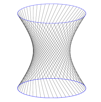
Figure 8.37: Formation of a hyperboloidal surface due to stereo wires.

The otherwise cylindrical surface of this wire layer turns into a hyperboloidal surface as shown in Fig.8.37. As a result, both the azimuthal angle and the radial position of the stereo wire becomes $z$-dependent:

$${\begin{array}[]{lll}\phi(z)&=&\phi(z=0)+\tan^{-1}\left[\left(\frac{2z}{L}\right)\tan\left(\frac{\Delta\phi}{2}\right)\right]\cr\rule{0.0pt}{21.52771pt}r(z)&=&\sqrt{\left(r(z=0)\right)^{2}+\left(z\tan\alpha\right)^{2}}\cr\rule{0.0pt}{17.22217pt}{}&=&\sqrt{\left(r(z=\pm L/2)\right)^{2}+\left(z^{2}-(L/2)^{2}\right)\tan^{2}\alpha},\end{array}}$$ (8.21)

where $z$ is measured from the middle of the chamber along the chamber axis .

This inhomogeneity distorts the electric field to some extent and limits the maximum possible stereo angle, thereby restricting the $z$ resolution $\sigma_{z}$. Fig.8.38 demonstrates how a single stereo cell structure deforms as one moves from one endplate to the other. This $z$-dependent geometrical deformation of the stereo cell is parametrized by a so called shrink factor and imposes another important restriction on the possible range of stereo angles.

Figure 8.38: Exaggerated illustration of the stereo-cell formation through rotation by an angle $\Delta\phi$ and its deformation along the wires. $ABCD$ and $A_{1}B_{1}C_{1}D_{1}$ are the cross sections of a single stereo cell at the end plates $(z=\pm L/2)$. $A_{2}B_{2}C_{2}D_{2}$ is that of the same stereo cell in-between $(-L/2~{}<~{}Z<~{}+L/2)$.

The shrink factor $f(z)$ is defined to be the ratio $A_{2}B_{2}(z)/AB(z=\pm L/2)$ in Fig.8.38 and is readily derived from Eqs.8.20 and 8.21:

$${\begin{array}[]{lll}f(z)&=&\frac{r_{B}(z)-r_{A}(z)}{r_{B}(z=\pm L/2)-r_{A}(z=\pm L/2)}\cr\rule{0.0pt}{30.1388pt}&=&\sqrt{1+\left(\frac{z^{2}-(L/2)^{2}}{L^{2}}\right)4\sin^{2}\left(\frac{\Delta\phi}{2}\right)}\cr\rule{0.0pt}{30.1388pt}&=&\frac{\sqrt{R^{2}+\left(z^{2}-(L/2)^{2}\right)\tan^{2}\alpha}}{R},\end{array}}$$ (8.23)

where $R=r(z=\pm L/2)$ and $f(z=\pm L/2)=1$ by definition.

It is a common practice to use pairs of stereo super-layers ($V$ and $U$) with alternating stereo angles ($\pm\alpha$) interleaved with axial super-layers ($A$). In this case, the inhomogeneity is more serious for the gap between a stereo super-layer ($V$) and the adjacent axial super-layer ($A$) just inside. The minimum gap attained at the middle point of the chamber has to be large enough for stable operations of the chamber.

8.3.3 A Possible Central Tracker

Chamber Design

Applying the general design principle explained above to the JLC case, we obtained the following basic parameters for a possible JLC central tracker: $B=2~{}T$, $r_{in}=45~{}{\rm cm}$, $r_{out}=230~{}{\rm cm}$, $L=460~{}{\rm cm}$, $n~{}=~{}80$, and $\sigma_{r\phi}=100~{}\mu{\rm m}$. The tracker consists of 6 axial and 10 stereo super-layers, each having 5 anode wires, arranged with increasing $r$ in the following order: $AVUAVUAVUAVUA$, where $A$, $V$, and $U$ again denote an axial super-layer, stereo super-layers with stereo angles of $+\alpha$ and $-\alpha$, respectively. The gap between adjacent super-layers is correlated with the stereo angle and is equal to either $4.0$ or $5.0~{}{\rm cm}$ at the endplates, depending on its radial location: the $U$-to-$A$ and the $V$-to-$U$ gaps are equal to $4.0~{}{\rm cm}$, while the $A$-to-$V$ is set at $5.0~{}{\rm cm}$ (see Fig.8.40).

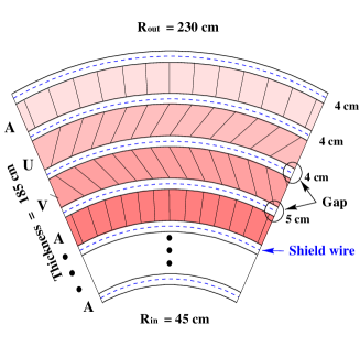
Figure 8.39: A possible super-layer layout for the central tracking system of the JLC.

Figure 8.40: A typical geometry of a single cell: the circles ($\circ$) and ($\bullet$) correspond to sense and potential wires, respectively.

In the current design, there is a layer of shielding wires in each gap between adjacent super-layers, in order to electrostatically isolate different super-layers. These shielding wires in a $V$-to-$U$ gap will have the same stereo angle ($\alpha$) with the $V$ wires. On the other hand, the shielding wires in $A$-to-$V$ or $U$-to-$A$ gaps will have half the stereo angle of the adjacent stereo super-layers ($\pm\alpha/2$). Note also that the stereo angle varies even within a single jet cell, according to Eq.8.20.

A possible cell design is shown in Fig. 8.40. The cell has $5$ sense wires spaced $1~{}{\rm cm}$, with each surrounded by ground wires in the sense wire plane and grid wires placed $5~{}{\rm mm}$ away from it. The two dummy sense wires at the both ends of the sense wire plane are placed to stabilize the upper- and the lower-most sense wires. The maximum drift length depends on the radial position of each sense wire and has a typical value of $5~{}{\rm cm}$. The drift field is produced by $10$ field shaping wires whose potentials change linearly and cathode wires that cover the end of the drift region. The high voltages on the wires will be chosen so as to get as uniform a drift field as possible with minimum electrostatic forces, while keeping a reasonable gas gain for a chamber gas mixture of $90\%{\rm CO_{2}}$ and $10\%$ Isobutane.

Questions to be Answered

The chamber parameters described above lead us to the following list of questions:

1. Can we control gravitational and electrostatic sags for 4.6m-long wires?

2. Is tension drop controllable for $Al$ wires?

3. Can we stably operate 4.6m-long stereo cells?

4. Can we achieve a spatial resolution of $100\mu{\rm m}$ everywhere in this big chamber?

5. Can we achieve 2-track separation better than $2{\rm mm}$?

6. Is gas gain saturation observed for cool gas mixtures no problem?

7. Is Lorentz angle small enough to allow straight cells?

8. Is neutron background ($\sim$2k hits/train for $B=2$T[34]) no problem? How big is the signal charge for a single neutron hit? Is there any dead time expected?

These questions naturally comprise our R&D items.

Let us begin with the first two questions which have to do with mechanical stability of the chamber.

Mechanical Stability

Figure 8.41: $4.6~{}{\rm m}$ CDC test chamber with wire position measurement system.

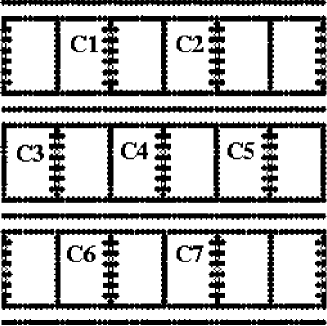
Figure 8.42: Cell layout of our $4.6~{}{\rm m}$ long test chamber.

In order to investigate mechanical stability of a drift chamber with very long wires, we have built a $4.6~{}{\rm m}$ long test chamber (see Fig. 8.42). We have also been developing a software program to predict wire displacement, knowing the cell structure, wire tension, and high voltage on each wire. The validity of the prediction has to be proved experimentally. We have developed a wire tension and position measurement system and measured wire tensions, gravitational and electrostatic sags for the $4.6~{}{\rm m}$ long test chamber. The results of the measurements were then compared with the predictions.

Our $4.6~{}{\rm m}$ long test chamber has seven identical cells with the cell parameters which approximate those of the aforementioned possible JLC central tracker. The layout of the seven cells is shown in Fig. 8.42.

The cell design is shown in Fig. 8.43-(a) which also specifies our wire naming convention to be used hereafter.

     

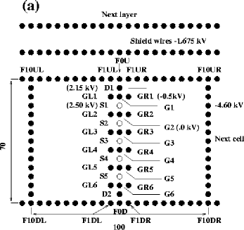
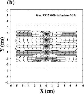
Figure 8.43: (a) possible small jet cell structure and (b) corresponding drift lines ($B$ = 0 T).

The cell has $5$ sense wires ($S1$ to $S5$) held at $2.5~{}{\rm kV}$ and spaced $1~{}{\rm cm}$, with each surrounded by ground wires ($G1$ to $G6$) in the sense wire plane and grid wires ($GL1$ to $GL6$ and $GR1$ to $GR6$) at $-0.5~{}{\rm kV}$ placed $5~{}{\rm mm}$ away from it. The two dummy sense wires ($D1$ and $D2$) at the both ends of the sense wire plane are held at $2.15~{}{\rm kV}$ and stabilize the upper- and the lower-most sense wires ($S1$ and $S5$). The maximum drift length is $5~{}{\rm cm}$ where the drift field is produced by $10$ field shaping wires ($F1**$ to $F10**$) whose potentials change linearly in this order from $-0.5~{}{\rm kV}$ to $-4.6~{}{\rm kV}$, and by left and right edge field wires held at $-4.6~{}{\rm kV}$. The wire diameter is $30~{}\mu{\rm m}$ for sense wires and $125~{}\mu{\rm m}$ for the others. The high voltages on the wires were chosen so as to get as uniform a drift field as possible with minimum electrostatic forces, while keeping a reasonable gas gain for a chamber gas mixture of $90\%{\rm CO_{2}}$ and $10\%$ Isobutane. Fig. 8.43-(b) plots the drift lines and isochrones calculated with a drift chamber simulation program GARFIELD [31]. Unless otherwise stated, wires we are going to deal with belong to the central cell ($C4$).

Before stringing wires, we surveyed the endplates to check their machining precision and found that the standard deviation of the actual wire hole positions from the nominal ones to be less than $8.2~{}\mu{\rm m}$. The sense wires are gold-plated tungsten and all the other wires are gold-plated aluminum. The reason for this choice of Al as the wire material is to minimize the total wire tension so as to reduce the thickness of the chamber endplates as required by endcap calorimeters. The wire stringing took us three weeks.

gravitational and electrostatic sags

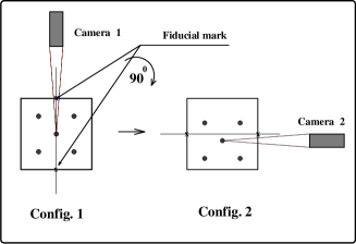
Figure 8.44: Principle of gravitational sag measurements.

Fig. 8.44 illustrates our measurement scheme of the gravitational sag of a wire. The measurement goes as follows. Using the vertical camera, we first put fiducial marks on the chamber windows in such a way that the line connecting them passes through the wire in question (configuration 1 in Fig. 8.44). Then we rotate the test chamber by 90^∘ and determine the wire deflection due to gravitational sag by measuring the wire position relative to the line connecting the fiducial marks, using the horizontal camera (config.2 in Fig. 8.44). We measured the gravitational sags 1.5 years after the wire stringing. The average gravitational sags for field and sense wires were 600$\mu$m and 353$\mu$m, respectively.

Our measurement scheme of electrostatic sag is sketched in Fig. 8.45. We first get a wire in sight on both the horizontal and vertical cameras with high voltages off. Then we measure the horizontal ($\Delta$X) and vertical ($\Delta$Y) displacements in the camera screens after turning on the high voltages. Notice that the camera stays at rest during the measurement and the measurement accuracy is determined completely by the wire image resolutions on the screens (there is no tilt angle effect here). The overall accuracy for the electric sag measurement was estimated to be $5~{}\mu{\rm m}$. The wire stability in the electrostatic field has been checked by turning on and off the high voltages several times. We found no instability, meaning that the wires always return to the same positions of equilibrium.

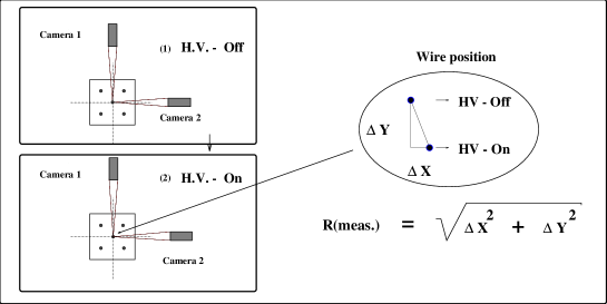
Figure 8.45: Schematic view of the electrostatic sag measurements.

Figs.8.46 and 8.47 illustrate the wire deflections in our $4.6~{}{\rm m}$ test chamber due to gravitational and electrostatic forces. In the figures an original position ($\bigtriangledown$) is the initial position of a wire at the end plates. On the other hand, denoted as gravitational sag (  ) and electric sag ($\star$) are the measured positions of the wire under the gravitational force before and after applying high voltages, respectively. Called f͡irst iteration ($\circ$) is the calculated value of the wire deflection in the electrostatic field when other wires are at the positions after the gravitational sags. The input parameters for the second iteration ($\bullet$) are the new wire positions from iteration 1.

In Fig.8.46 we compare the measurements and predictions for a few field wires which are on the left and right sides of the sense wire plane. There is a good agreement not only in the magnitude of deflection but also in its direction for each one of these field wires. It is clear that the prediction from the second iteration is better.

Results of the predictions and measurements for sense wires $S1$ and $S2$ are shown in Fig.8.47. There is a noticeable left-right asymmetry in the measurements with respect to the original sense wire plane, which could not be reproduced by the calculation. Probably the source of such an asymmetry can be attributed to the influence of the other cells which might have some asymmetry in wire tensions, since they were strung over a finite period of time.

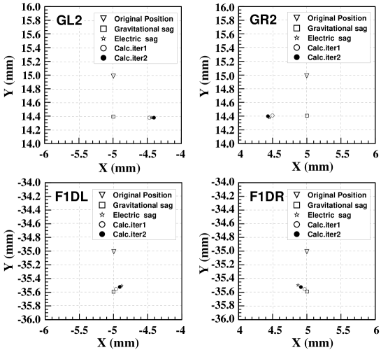
Figure 8.46: Measured positions of some representative field wires at the endplates ($\bigtriangledown$), with gravitational sags (  ) before and ($\star$) after electrostatic sags, compared with calculations: iterations $1$($\circ$) and $2$ ($\bullet$).

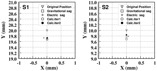
Figure 8.47: Same as Fig. 9 for the worst ($S1$) and a typical ($S2$) sense wires.

wire tension drop problem

Almost all methods of wire tension measurements are based on the same basic principle [28] and ours is no exception. We excite oscillations of a wire at its resonant frequency, and then determine the tension $T$ by using the following relation:

$$T=4\rho\cdot L^{2}\cdot f^{2},$$ (8.24)

where $f$ is the fundamental resonant frequency. The results are shown in Figs. 8.48-(a) and -(b) for field and sense wires, respectively, as functions of the time measured from the day of wire stringing.

     

Figure 8.48: Tension versus time for (a) field and (b) sense wires.

There is still a tension drop of about 10%/year for gold-plated Al field wires unlike gold-plated W sense wires which now reach a tension plateau. Since this poses a potential problem and requires a better wire material, we are continuing wire material studies.

We now move on to question 3 which is the operational stability issue discussed in detail in [24] [29].

Operational Stability

surface field variation due to stereo wires

As shown earlier, the wires belonging to a stereo layer form a hyperboloidal surface. Consequently, any stereo cell shrinks as one moves from an endplate to the middle of the wires. The resultant shrink factor is shown in Fig.8.50 for all of the 10 ($V$,$U$) stereo super-layers of the possible JLC central tracker.

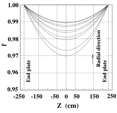
Figure 8.49: Shrink factor ($f$) as a function of $z$ for all of the 10 super-layers: from the bottom to the top, the lines correspond to super-layers ordered in the radial direction.

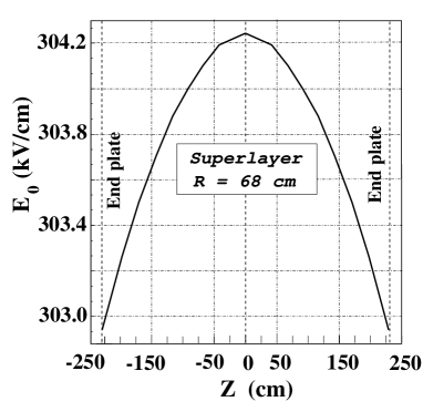
Figure 8.50: Surface field as a function of $z$ for a sense wire in the innermost stereo super-layer at $r=68~{}{\rm cm}$.

The variation of the shrink factor $\Delta f/f$ is at most $3~{}\%$ observed for the innermost stereo super-layer which has $r=68~{}{\rm cm}$ and $\alpha=75~{}{\rm mrad}$. The $z$-dependent geometrical deformation of the stereo cell induces variation of the surface field on the sense wires in it, thereby introducing gain nonuniformity along the wires. We calculated the surface field variation on the sense wires, using the drift chamber simulation program, GARFIELD. The size of the cell structure depends on the shrink factor $f$ and varies also with the radial position or the super-layer that the cell belongs to. Fig.8.50 plots the calculated surface fields against the $z$ coordinate. The maximum variation of the surface field is $\Delta E/E\simeq 0.43~{}\%$.

surface field variation due to wire sags

In addition to the stereo geometry, there is another source of geometrical deformation of the cell structure that is the wire sags due to gravitational and electrostatic forces on the wire. These gravitational and electrostatic sags also contribute to the surface field variation and are common to both axial and stereo wires. It suffices to investigate the effects of these wire sags for axial wires only. We, therefore, calculate the surface field variation with GARFIELD, using as input the electrostatic and gravitational sags actually measured as the difference of the wire coordinates at $z=\pm L/2$ (wire ends) and $z=0$ (mid point) for a $4.6~{}{\rm m}$-long test chamber[22]. The maximum wire-sag-induced variation of the surface field is $\Delta E_{0}/E_{0}\simeq 1.4~{}\%$. It should be emphasized that the fact that the field variation is comparable with those from the stereo geometry for our example is largely due to the use of Aluminum field wires. We can in principle reduce the field variation from the gravitational and electrostatic sags, by optimizing the wire materials and by stringing these wires with higher tensions. On the other hand, the limitation coming from the stereo geometry is inherent in any stereo chamber and is unavoidable.

gas gain variation along the wires

Now that we know the surface field variation along any wire, we can study its $z$-dependent gas gain variation and discuss the operation feasibility of the chamber, provided that the relation of the surface field to the gas gain is known. Conversely, the stereo angle should be so determined to make the gain variation acceptable.

We have measured the gas gain for the ${\rm CO}_{2}(90\%)$-Isobutane $(10\%)$ mixture, by using a single wire proportional counter[29]. The counter is made of an aluminum cathode tube with a $10~{}{\rm mm}$ inner diameter and a gold-plated tungsten anode wire with a $30~{}\mu{\rm m}$ diameter. For the ⁵⁵Fe $X$-rays ($5.9~{}{\rm keV}$) and ⁹⁰Sr $\beta$-rays, the charges collected on the anode within $1~{}\mu{\rm sec}$ were measured as a function of the applied voltage.

Gas gain measurements for different Isobutane concentrations (5%, 10%, and 15%) have been made. The results for $X$-rays are shown in Fig.8.52. The gas gain increases as the Isobutane concentration becomes bigger.

Figure 8.51: HV dependence of the charges collected in $1.0~{}\mu{\rm s}$ for $X$-rays with three different concentrations of the ${\rm CO}_{2}$/Isobutane mixture.

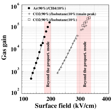
Figure 8.52: Gas gain as a function of the surface field for the Single Wire Tube with the ${\rm CO}_{2}(90\%)$-Isobutane $(10\%)$ gas mixture.

The measured data on the gain variation as a function of the surface field are fitted in Fig.8.52 to the following empirical formula:

$$\ln G=a+bE_{0},$$ (8.25)

where $a$ and $b$ are the parameters to be determined. From these data, we obtain the following relation:

$$\frac{\Delta G}{G}=(15\sim 20)\left(\frac{dE_{0}}{E_{0}}\right)$$ (8.26)

around $E_{0}\simeq 300~{}{\rm kV/cm}$, where the gas gain is about $10^{5}$.

By combining these results with the surface field variations calculated above, we estimate the gain variation of the stereo wire due to the stereo geometry to be at most $8~{}\%$ which is acceptable.

The surface field variation due to the wire displacements induced by gravitational and electrostatic forces for our $4.6~{}{\rm m}$ test chamber could give rise to some additional gain variation as large as $25~{}\%$ at worst. The wire displacements can, however, be reduced by appropriate choices of wire materials enduring higher tensions, a higher gain gas mixture allowing lower high voltages on sense wires, etc. On the other hand, the gas gain variation due to the stereo geometry is irreducible without geometry redesigning.

Finishing up with the stability questions, let us move on to questions 4 and 5 concerning required chamber performance [23].

Expected Chamber Performance

spatial resolution

Can we actually achieve the required spatial resolution over the full length of the $4.6~{}{\rm m}$-long chamber? In order to confirm this, we studied the performance of the test chamber using cosmic rays [23]. Here again we concentrate our attention on the central cell. Signals from the 5 sense wires belonging to the central cell were amplified by a pre-amplifier, which is mounted on an end-plate of the test chamber, and by a post-amplifier after passing through a $5~{}{\rm m}$-long twisted pair cable. The gains of the pre-amplifier is about $200~{}{\rm mV/pC}$ for the short pulse. The signal from the post-amplifier is fed to an 8-bit flash-ADC (REPIC RPC-250), which has a $500~{}{\rm MHz}$ sampling frequency over a $16~{}\mu{\rm sec}$ time window. Any pulse from $0$ to $-1~{}{\rm V}$ is chopped into $2~{}{\rm nsec}$ time slots and converted to a train of digits in the interval of $0$ to $255$ counts by this flash-ADC. The flash-ADC fully covers the maximum drift time of the test chamber (about $6~{}\mu{\rm sec}$) and provides a high enough sampling frequency to ensure a good enough resolution ($2~{}{\rm nsec}$ corresponding to $16~{}\mu{\rm m}$ drift equivalent).

The digitized pulse form is read out and recorded on a disk by a computer (NEC PC98) through a CAMAC system. Any pulse which continues longer than $120~{}{\rm nsec}$ above the threshold (pedestal+3 counts) was regarded as a signal pulse. The arrival time of the signal pulse was determined by its leading edge at which the pulse height exceeded the threshold. To convert the drift time to the drift length, we use the $x$-$t$ relation calculated with GARFIELD for each wire. The validity of the calculated $x$-$t$ relation was experimentally confirmed by comparing the drift velocity given by GARFIELD with independent drift velocity measurements.

We selected events demanding that the 4 out of the 5 sense wires excluding the one to study had to have hits and made a reference track. We then calculated, on an event-by-event basis, the residual of each hit on the wire to look at as the distance from the reference track consisting of the 4 hits. The so-obtained residual distribution for the central wire ($S3$) is plotted in Fig. 8.53-(a) against the drift length for tracks passing through the central cell ($C4$) in the middle of the wires, with the two trigger counters vertically aligned so as to primarily sample tracks perpendicular to the sense wires (for our naming convention, see Fig. 8.43(a)).

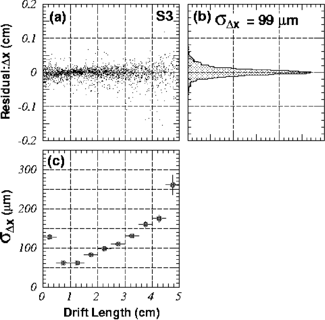
Figure 8.53: Residual for $S3$ at the center of the test chamber (a) plotted against drift length, (b) its projection to the vertical axis, and (c) the standard deviation of the residual distribution as a function of the drift length.

Fig. 8.53-(c) shows the one-standard-deviation ($1$-$\sigma$) width of the residual distribution as a function of the drift distance. The width is less than $100~{}\mu{\rm m}$ for a drift length less than $2.5~{}{\rm cm}$, except for the vicinity of the sense wire. It becomes, however, gradually worse up to about $200~{}\mu{\rm m}$ towards the edge of the drift volume. Fig. 8.53-(b) is the projection to the vertical (residual) axis, demonstrating the overall residual distribution.

The edge wires ($S1$ and $S5$) have wider distributions. This is due to the reference track extrapolation error for $S1$ and $S5$ being much larger than the interpolation error for $S2$ to $S4$. In order to estimate the intrinsic spatial resolution of each wire we calculated the track error as a function of the drift distance and subtracted it in quadrature on a bin-by-bin basis. We then averaged the resultant resolution over the drift distance to compensate the acceptance non-uniformity. The so-obtained overall intrinsic spatial resolutions for individual sense wires are summarized in Table 8.5. Inspection of the table tells us that the overall resolutions are around $100\mu{\rm m}$, approximately satisfying our performance goal at least locally.

A similar analysis was carried out for tracks passing though the central cell near the both ends of the wires, in order to make sure that the performance goal be satisfied over the full length of the chamber. Though the spatial resolutions became slightly worse, they are still close to $100~{}\mu{\rm m}$ as listed in Table 8.5.

Table 8.5: Summary of spatial resolutions.

Wire Number	Center	Ends	Inclined
S1	$117\pm 23(\mu m)$	$163\pm 75(\mu m)$	$94\pm 38(\mu m)$
S2	$103\pm 7(\mu m)$	$136\pm 52(\mu m)$	$95\pm 15(\mu m)$
S3	$103\pm 9(\mu m)$	$120\pm 22(\mu m)$	$102\pm 19(\mu m)$
S4	$98\pm 9(\mu m)$	$119\pm 22(\mu m)$	$90\pm 19(\mu m)$
S5	$109\pm 16(\mu m)$	$132\pm 45(\mu m)$	$105\pm 39(\mu m)$

The intrinsic resolutions may also depend upon the incident angle of a track to the sense wires. In order to investigate this effect, we set the two trigger counters in the middle of the chamber but slightly displaced so as to primarily sample inclined tracks having an incident angle of around $45^{\circ}$ to the wires. This incident angle ($45^{\circ}$) corresponds to the maximum dip angle with the full number of sense wires for the possible JLC central tracker. The width of the residual distributions were translated into overall intrinsic spatial resolutions after the track error and acceptance corrections, and are summarized also in Table 8.5. We thus confirmed that a spatial resolution of about $100\mu{\rm m}$ up to an incident angle of $45^{\circ}$.

The efficiency for each wire was calculated as a function of the drift distance to be the fraction of tracks with actual hits on the wire in a $5$-$\sigma$ window. Fig. 8.54 is the results of the calculations, for an oxygen contamination in the chamber gas of about $60~{}{\rm ppm}$.

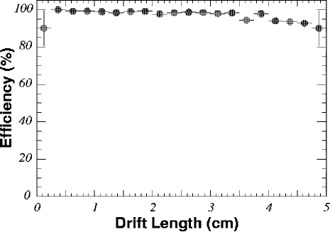
Figure 8.54: Efficiency of the central sense wire ($S3$) as a function of the drift distance.

The efficiency stays flat above $95\%$ except in the last several bins close to the edge of the drift volume. The slight drop towards the edge is primarily coming from the drift electron absorption due to the oxygen contamination.

To investigate the effect of the oxygen contamination in the chamber gas, we compared the chamber performance for two different oxygen contaminations, $60~{}{\rm ppm}$ and $120~{}{\rm ppm}$. The oxygen molecules, being electro-negative, capture some electrons drifting towards a sense wire and make the signal pulse smaller as the drift length gets longer. We chose the chamber gas with a slow drift velocity to reduce the effect of the diffusion of the drift electrons. This choice made the chamber more sensitive to a small contamination from electro-negative gases.

The pulse hight becomes smaller with the drift distance due to the diffusion. However, the total charge of the pulse must stay the same, as long as there is no drift electron loss. Plotted in Fig. 8.55-(a) is the integrated signal charge on $S3$ against the drift distance for an oxygen contamination of $60~{}{\rm ppm}$. The signal charge gets smaller as the drift distance becomes longer, indicating that an electro-negative gas at work. In order to confirm this effect, we intentionally increased the oxygen contamination to $120~{}{\rm ppm}$ and measured the drift-length dependence of the signal charge. As seen in Fig. 8.55-(b), the pulse charge rapidly decreases with the drift distance and vanishes down below the threshold at the large drift distance, suggesting a total loss of drift electrons.

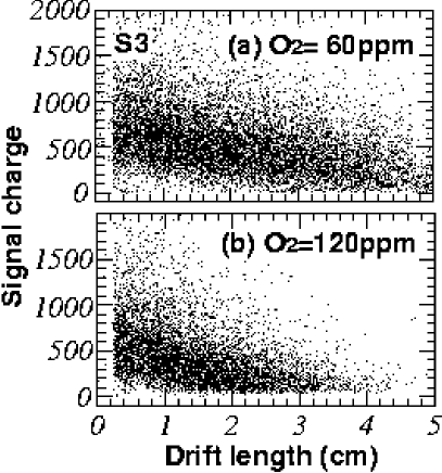
Figure 8.55: (a) Pulse charge on the central sense wire ($S3$) as a function of the drift distance for an oxygen contamination of $60~{}{\rm ppm}$. (b) Same as (a) but for an oxygen contamination of $120~{}{\rm ppm}$.

This effect not only diminishes the wire efficiencies but may also deteriorate the spatial resolutions in the large drift-length region. As a matter of fact, Fig. 8.53 shows a resolution increment with the drift distance larger than naively expected from diffusion. It may be explained by the drift electron loss due to the oxygen contamination. A better performance can thus be expected if the oxygen contamination is reduced.

In order to verify this expectation, we studied the effect of the oxygen contamination with a smaller test chamber for which further reduction of oxygen contamination is possible. The smaller test chamber, hereafter called ”baby chamber” has three jet-cells with the same wire layout as the 4.6 m chamber but with a shorter wire length of 40 cm (see Fig. 8.56).

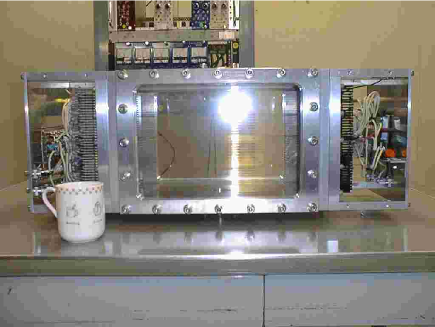
Figure 8.56: Baby chamber

Using the baby chamber and essentially the same data taking system as used above for the 4.6 m test chamber, we took cosmic ray data. We then followed the same data analysis procedure as above and calculated the wire efficiency for the cosmic ray tracks that passed the chamber with an incident angle of nearly $90^{\circ}$. Fig. 8.57 shows the efficiency of the central sense wire as a function of the drift distance for oxygen contaminations of $120~{}{\rm ppm}$ and $20~{}{\rm ppm}$, respectively.

     

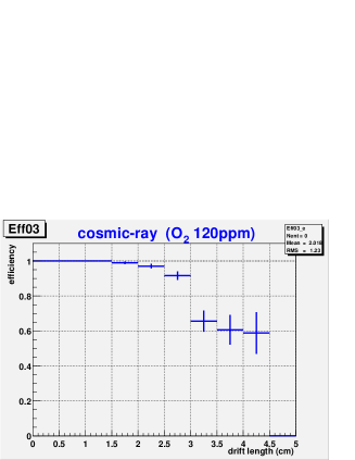
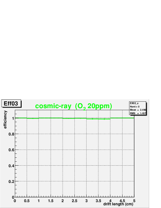
Figure 8.57: Efficiency of the central sense wire ($S3$) as a function of the drift distance (baby chamber): O₂ contaminations of 120 ppm (left) and 20 ppm (right).

In the case of $120~{}{\rm ppm}$ we see a sharp efficiency drop towards the edge while for the oxygen contamination of $20~{}{\rm ppm}$ the efficiency stays almost $100\%$ everywhere. The sharp efficiency drop observed for $120~{}{\rm ppm}$ is coming from the drift electron absorption due to the relatively high oxygen contamination, which is obvious from Fig. 8.58 showing the integrated signal charge on the central sense wire as a function of the drift distance: the signal charge gets significantly smaller for $120~{}{\rm ppm}$ than for $20~{}{\rm ppm}$ as the drift distance becomes longer.

     

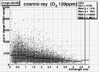
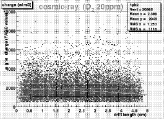
Figure 8.58: Pulse charge on the central sense wire ($S3$) of the baby chamber as a function of the drift distance for oxygen contaminations of $120~{}{\rm ppm}$ (left) and $20~{}{\rm ppm}$ (right).

We obtained similar results for other sense wires. The attachment rate of drift electrons was evaluated from the observed charge attenuation as a function of drift distance and the known drift velocity. In Fig. 8.59 our measurement is compared with that calculated using the three-body attachment coefficient measured by J.L. Pack and A.V. Phelps [30].

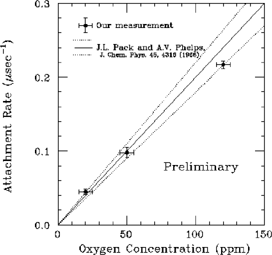
Figure 8.59: Attachment rate as a function of oxygen concentration (preliminary).

Being encouraged by the drift-distance dependence of the wire efficiency for $20~{}{\rm ppm}$, we then studied the spatial resolution per wire. The analysis procedure was the same as with the 4.6 m test chamber: we calculated the residual for the wire in question on the event-by-event basis, using a reference track drawn with the hits on the other 4 wires. We then subtracted the track error from the standard deviation of the residual distribution to obtain the spatial resolution. Fig. 8.60 plots the spatial resolution of the central sense wire against the drift length for $20~{}{\rm ppm}$, which shows much more reasonable drift length dependence compared to Fig. 8.53.

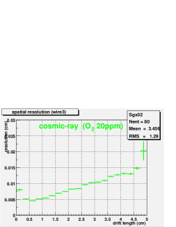
Figure 8.60: Spatial resolution of the central wire of the baby chamber as a function of the drift length (preliminary).

The oxygen contamination of the gas would not be a serious problem in the real chamber since the oxygen level is planed to be kept lower than 10 ppm with better gas tightness.

two-track separation

Next question is whether we can reproduce the single track results above in a multi-track environment. In order to answer this question, we have carried out beam tests of the baby chamber, using $e^{+}e^{-}$ pairs produced by gamma conversions at an $Al$ converter. The $e^{+}e^{-}$ pairs provided closely spaced 2 tracks at our disposal in the chamber and their signals were read out with the same readout electronics as used for the cosmic ray tests described above.

Fig. 8.61-(a) shows FADC signals from 10 wires, 5 of which belongs to the upstream and the other 5 to the downstream cells, for a typical 2-track event. We can see two closely spaced hits on each wire. We calculated the 2-hit separation efficiency for each wire in a cell, demanding two reference tracks made of hits on the 4 reference wires other than the wire to study. The two tracks define the 2-track distance and the expected hit position for the second track on the wire in question. Figure 8.61-(b) plots the efficiency for the second hit as a function of the 2-track distance in the case of normal incidence.

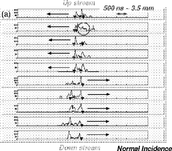
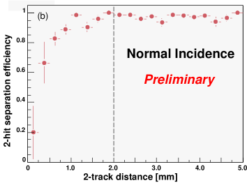
Figure 8.61: (a) FADC signals as a function of time (500 ns/division) for a typical 2-track event. The arrows indicate the drift direction. (b) 2-hit separation efficiency as a function of 2-track distance (preliminary).

Although the result looks promising, it is still preliminary and more studies are needed to investigate possible space charge effects due to the small diffusion nature of our gas mixture. We will return to this problem later in the subsection for space charge effect.

particle identification

Particle identification through energy loss ($dE/dx$) measurements in a drift chamber is a well established technique and could be additional information provided by the JLC-CDC. However the primary demand to the CDC is high spatial resolution to be achieved with a wire gain as high as $10^{5}$ while $dE/dx$ measurements require a low gain in order to assure the proportionality of the collected charge to the total number of ionization acts by a charged particle. When the wire gain is high this proportionality is lost because the positive ions created in the avalanche process initiated by a given drift electron effectively reduce the electric field near the sense wire surface and then prevent the normal growth of avalanches initiated by subsequent electrons (space charge effect). In addition, the small diffusion of drift electrons (especially along the wire direction) in a CO₂-based gas mixture may cause a severe space charge effect since the drift electrons get amplified in small surface area on the sense wire.

In order to evaluate the particle identification capability of the JLC-CDC, we carried out $dE/dx$ measurements by irradiating the baby chamber with particle beams ($e$, $\pi$ and $p$) at the 12-GeV KEK proton synchrotron (KEK-PS). Fig. 8.62 shows the normalized energy loss as a function of $\beta\gamma$ for different beam incident angles. The beam is parallel with the sense-wire plane and the incident angle ($\theta$) here is defined to be $0^{\circ}$ when the beam is perpendicular to the wire direction. The energy loss was determined by averaging 80%-retained truncated means of 10 samples. The normalized $dE/dx$ decreases for smaller beam angles especially in the low $\beta\gamma$ region. This indicates that the space charge effect does affect the $dE/dx$ measurements for highly ionizing tracks nearly perpendicular to the sense wires.

Figure 8.62: Relative energy loss as a function of $\beta\gamma$. The $dE/dx$ values are normalized to that of 0.5 GeV/c pions and corrected for incident angles (preliminary).

Since the present design of the JLC-CDC assumes 16 layers of the 5-sense-wire jet cells in the radial direction, 80 samples of $dE/dx$ measurement are expected for a single track. In order to estimate the particle identification capability with this configuration, we applied the 80%-retained truncated mean method to the 80 $dE/dx$ measurements in a set of 8 consecutive events (tracks), each with 10 samples, recorded by the baby chamber. The result for $\pi-p$ separation at 1 GeV/c and $\theta=0^{\circ}$ is shown in Fig. 8.63. The obtained figure of merit of separation is $S\equiv 2\cdot\left|(dE/dx)_{A}-(dE/dx)_{B}\right|/(\sigma_{A}+\sigma_{B})=4.6$.

In spite of the possible space charge effect, the $dE/dx$ information may still provide a useful means for particle identification.

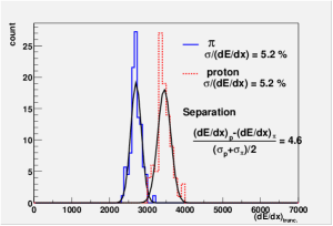
Figure 8.63: Expected $\pi-p$ separation for 80 samples at 1 GeV/c (preliminary).

Space Charge Effect

local space charge effect

However, not to mention two-track separation capability, the space charge effect in multi-track environment may significantly affect the chamber performance including spatial resolution and particle identification by $dE/dx$ measurements.

We thus studied the effect of local space charge on gas amplification with parallel laser beams ($\lambda$ = 266 nm) created by a splitter (quartz plate), which simulate two closely spaced strings of ionizations produced by two charged particles in a jet. The beam distance was controlled by changing the thickness of the quartz plate. The laser beams were injected into a single-wire drift chamber with a 50-mm drift space used originally for the Lorentz angle measurement [25].

Figure 8.64: Wave forms for double laser beams.

In Fig. 8.64, typical wave forms for double laser beams at $x_{1}$ = 10 mm is shown for $\Delta x$ = 2.2 mm and $\Delta z$ = 0 mm, where $x_{1}$ denotes the drift distance for the first signal, $\Delta x$ ($\Delta z$) is the beam distance in the drift (wire) direction, and the beams are parallel with the $y$-axis. The two laser tracks are clearly separated. The FWHM of the signal is 80 ns, which corresponds to the electron drift distance of 600 $\mu$m.

The signal charges were obtained by integrating the wave form. It should be noted that intensities of the two laser beams are different because of the unequal splitting. The gain reduction factor of the second signal due to the existence of the first one was obtained as $Q_{2}(Q_{1})/Q_{2}(Q_{1}=0)$, where $Q_{1}$ and $Q_{2}$ are the integrated charges for the first and the second signals, respectively. $Q_{2}(Q_{1}=0)$ was obtained by blocking the first laser beam. The values of $Q_{1}$ and $Q_{2}$ were measured for each event and the mean values of 300 events were used to obtain the reduction factor. In Fig. 8.65, we plot it as a function of the first signal charge for different beam distances in the drift direction. On the other hand, Fig. 8.66 shows the reduction factor as a function of the distance along the wire. These figures tell us that

• The gain reduction due to the space charge depends on the size of the first signal as naively expected;

• This gain reduction is a local effect on the sense wire surface which appears only within a limited distance from the first avalanches;

• This local paralysis is sustained for a long time because of the low mobility of positive ions.

The timing quality of the second signal, which is directly reflected to the spatial resolution, is now under study.

Figure 8.65: Gain reduction factor of the second signal as a function of $Q_{1}$ for $\Delta z$ = 0 mm and $\Delta x$ = 6.1 mm, 5.3 mm, 4.6 mm, 3.0 mm and 2.2 mm, measured with $x_{1}$ = 10 mm and $E$ (electric field strength on the sense wire surface) = 273 kV/cm (preliminary).

Figure 8.66: Gain reduction factor of the second signal as a function of $\Delta z$ measured with $x_{1}$ = 10 mm, $\Delta x\sim$ 4 mm and $E$ = 238 kV/cm. (preliminary)

global space charge effect

Another category of the space charge effect may set in when the beam background is severe and positive ions are accumulated in the sensitive volume of the chamber. Not to mention the wire gain reduction, the positive ions would cause significant distortion of the otherwise uniform electric field in the drift space. In that case the measured coordinates on charged tracks deviate from those which would result under circumstances free from positive ions (global space charge). It should be noted that the drift velocity in a CO₂-based gas is sensitive to the local electric field strength. These deviations would be dependent on both position and time, and could be comparable to, or larger than the spatial resolution expected of the JLC-CDC. Therefore it is possible that the global space charge effect devastatingly degrade the chamber performance.

In order to study the global space charge effect, we are now planning a small experiment using the baby chamber and a laser beam at KEK-PS. In the experiment the movement of the laser beacon tracks will be observed under the controlled intensity of defocused particle beam.

So much for the performance issues, let us now move on to question 7, concerning the magnitude of the magnetic field and how it affects the cell design.

Magnetic Field Effect

2 tesla design

The Lorentz angle, which is the angle between the drift direction of electrons under the influence of magnetic field and the direction of electric field, is one of the key parameters to determine the jet cell design. The existence of the magnetic field tilts drift lines by the Lorentz angle with respect to the electric field direction. If this angle is too big, drift lines for the edge wires hit top or bottom walls of the drift cell, thereby leading us to loss of detection efficiency.

Fig. 8.67 shows electron drift lines in a jet cell calculated by the chamber simulation program GARFIELD [31] (a) without and (b) with the magnetic field. The results indicates that the drift lines are completely contained in the cell at least up to a magnetic field of $2~{}{\rm T}$. There is, however, no systematic experimental data published for the Lorentz angles of ${\rm CO}_{2}$/isobutane gas mixtures, which makes difficult for us to test the reliability of our calculations using the GARFIELD program.

Figure 8.67: GARFIELD results of electron drift lines and isochrones in the JLC-CDC for the ${\rm CO}_{2}$/isobutane(90:10) gas mixture.

In order to confirm the results of the GARFIELD calculations and to verify the validity of our cell design, we have developed a Lorentz angle measurement system for cool gas mixtures, which have small Lorentz angles, and carried out systematic measurement for ${\rm CO}_{2}$/isobutane gas mixtures. The measurement system is characterized by the use of two laser beams to produce primary electrons and flash ADCs to read their signals simultaneously.

We measured the Lorentz angles for different ${\rm CO}_{2}$/isobutane gas mixtures. The results are shown in Figs. 8.68-(a), -(b), and -(c) as a function of the electric field for three mixing ratios: $(85:15)$, $(90:10)$, and $(95:5)$. At each electric field value in each figure, seven points are plotted, corresponding to, from bottom to top, seven magnetic field values: $0.0$, $0.3$, $0.5$, $0.75$, $1.0$, $1.2,$, and $1.5~{}{\rm T}$, respectively.

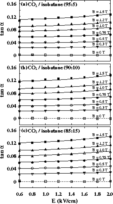
Figure 8.68: Tangent of the Lorentz angle ($\tan\alpha$) as a function of the electric field for ${\rm CO}_{2}$/isobutane mixtures of (a) (95:5), (b) (90:10), and (c) (85:15). Smooth curves are GARFIELD/MAGBOLTZ predictions.

Curves in Figs. 8.68-(a), -(b), and -(c) are predictions obtained with MAGBOLTZ-1 (version 1.16) through its GARFIELD interface, although its accuracy for the random velocity distribution of electrons is known to be limited under certain circumstances[32]. The loss of accuracy is caused by a decomposition of the velocity distribution function in Legendre polynomials, in which the lowest two or three terms are retained in the calculation. Therefore results given by the program may not be precise enough when the velocity distribution deviates far from isotropy or it has no axial symmetry as in the case of crossed electric and magnetic fields. On the other hand, our experimental condition seems to be favorable for application of MAGBOLTZ-1: electrons in ${\rm CO}_{2}$-based gas mixtures under a low electric field are nearly thermal, i.e. the velocity distribution is close to Maxwellian, and the axial symmetry of the velocity distribution holds to a good extent, because the momentum transfer cross section is fairly constant over the main portion of the electron velocity (energy) distribution. To confirm this we ran the Monte Carlo version (MAGBOLTZ-2, version 2.2[33]), which is free from the problems stated above though time-consuming, to simulate Lorentz angles for several electric and magnetic field combinations. The results were found to be consistent with those obtained with MAGBOLTZ-1.

We calculated the magnetic deflection coefficient ($\psi$) from the measured Lorentz angles and the drift velocities obtained without magnetic field. Fig. 8.69 shows the resultant $\psi$ as a function of electric field strength for the CO₂/isobutane(90:10) mixture at $B=1.5$ T, while Fig. 8.70 shows the drift velocity in the absence of magnetic field($v_{D}^{0}$). The values of $\psi$ were found to be close to unity within $\pm$ 5% for the whole range of the applied electric and magnetic fields and for all the gas mixtures used. The gas dependence of the Lorentz angle is shown in Fig. 8.71. The observed increase of the Lorentz angle with isobutane concentration is consistent with the increase of drift velocity and with $\psi=1$.

Figure 8.69: Magnetic deflection coefficient at $B=1.5$T as a function of the electric field for the ${\rm CO}_{2}$/isobutane(90:10) mixture.

Figure 8.70: Drift velocity at $B=0$ as a function of the electric field for the ${\rm CO}_{2}$/isobutane(90:10) mixture.

Figure 8.71: Isobutane concentration dependence of $\tan\alpha$ at $E=1.0~{}$kV/cm. The solid lines are GARFIELD/MAGBOLTZ predictions.

The current design of the JLC-CDC assumes operation under a magnetic field of $2.0~{}{\rm T}$. Figure 8.72 plots the Lorentz angle as a function of the magnetic field. The Lorentz angle is proportional to the magnetic field as long as $\psi=1$. We thus fit the data points below $1.5~{}{\rm T}$ to a straight line passing through the origin and extrapolate the line to $2.0~{}{\rm T}$, in order to estimate the Lorentz angle for the JLC-CDC. At $E=1~{}{\rm kV/cm}$ and $B=2~{}{\rm T}$ the extrapolated Lorentz angle is $\tan\alpha=0.159\pm 0.002$ for the ${\rm CO}_{2}$/isobutane(90:10) mixture. The shaded band above $1.5~{}{\rm T}$ indicates $1$-$\sigma$ extrapolation error interval. The solid line in the figure is the prediction of GARFIELD/MAGBOLTZ which is consistent with the extrapolation for $2~{}{\rm T}$.

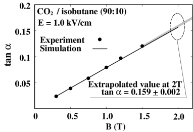
Figure 8.72: $\tan\alpha$ at $E=1.0$ kV/cm plotted against the magnetic field for the ${\rm CO}_{2}$/isobutane(90:10) mixture. The shaded band above $B=1.5$ T is the $1$-$\sigma$ bound for the straight-line extrapolation, while the solid line is the GARFIELD/MAGBOLTZ simulation.

higher magnetic field option

Motivated mainly by recent studies of beam-induced background[34], possibility of higher magnetic field is now under serious considerations. Our current cell design allows a magnetic field up to about $3~{}{\rm T}$. Since GARFIELD/MAGBOLTZ reproduces our Lorentz angle data very well, it is plausible that it continues to work well at around $3~{}{\rm T}$, too. It is, however, desirable to confirm this experimentally. We are thus planning to measure Lorentz angles at higher magnetic fields.

8.3.4 Summary

We have given affirmative answers to most of the basic R&D questions we raised in the introduction: in particular, we have demonstrated the possibility to achieve an average spatial resolution of $\sigma_{xy}\hbox{ \raise 3.0pt\hbox to0.0pt{$<$}\raise-3.0pt\hbox{$\sim$} }100~{}\mu{\rm m}$. Still remaining are those related to the gas gain saturation and space charge effects inherent in the gas mixtures having small diffusion coefficients, and the tension drop problem for $Al$ wires. The space charge effects are being studied using laser beams as well as charged particles, while wire material studies are in progress.

As discussed in the beginning of this chapter, there is a demand for a higher magnetic field from beam-related background reduction point of view. We are thus investigating possibilities to increase the magnetic field from $2$ T to $3$ T. If we could scale all the chamber parameters that have the dimension of length by a factor of 2/3, the chamber performance would stay unchanged. This is, however, impracticable since wire spacing, spatial resolution, and inner radius are difficult to scale, if not impossible. The expected performance of a $3$ T design, where these three parameters are kept unchanged, is discussed at the end of this chapter. In any case, any design change should be made consistently to the whole detector system, and should be justified by physics simulation studies. For this purpose, we started developing a full detector simulator with GEANT4, while brushing up the one based on GEANT3.

8.4 Performances of Tracking System

Vertexing Performance

Using a quick simulator, performance of the topological vertexing and the mass tagging method was studied. The topological vertexing algorithm was developed by the SLD group[35]. In this method, a tube of probability is defined along a particle trajectory. Since the probability is high when trajectories overlap, such points are selected as vertices. When a secondary or tertiary vertex is found, the $p_{t}$ corrected mass ($M_{corr}$) is calculated from the vertex mass ($M_{vtx}$) and the vertex momentum transverse to the flight direction of the vertex ($P_{T}$):

For the study, we generated quark pair events at the $Z$ pole. The events were clustered to two jets by using the JADE clustering algorithm. $Y_{cut}$ was varied so as to force clustering to two jets. When the production angle of the jet satisfied $|\cos\theta_{jet}|<0.8$, the tagging method was applied and efficiencies and purities were studied.

Fig. 8.73 shows the probability to find secondary vertices for $b\bar{b}$ events. The efficiency was about 90% and flat for a decay length greater than about 0.1 cm. The distribution of $M_{corr}$ is shown in Fig. 8.74 for jets whose secondary decay lengths are greater than 300 $\mu$m. We can see clear separation between $b$ quark jets and $c$ quark jets.

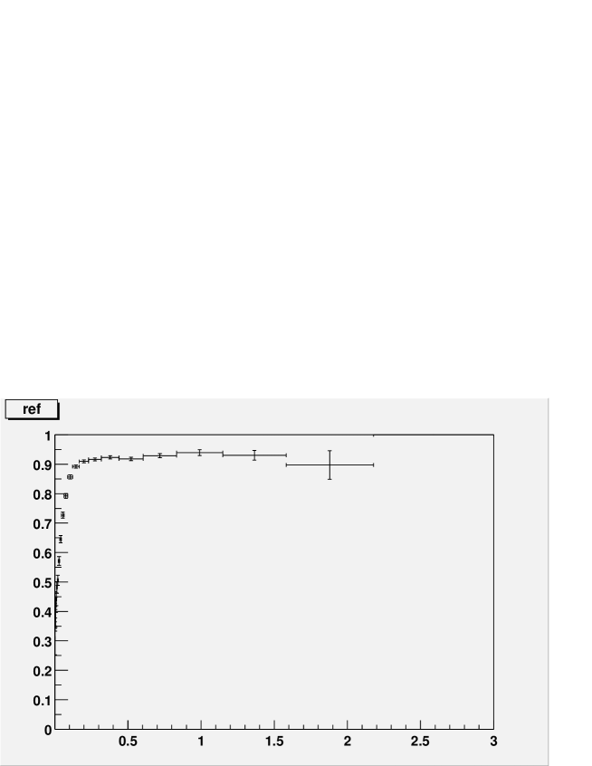
Figure 8.73: The efficiency to find secondary vertices in $b$-quark jets as a function of decay length (cm).

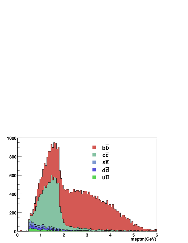
Figure 8.74: The $p_{t}$ corrected secondary mass ($M_{corr}$) distribution for each quark.

We tagged jets as $b$ when the decay length was greater than 300 $\mu$m and $M_{corr}$ was greater than the cut value. The purity and the efficiency of the $b$ tagging is shown in Fig. 8.75, which was obtained by changing the cut value from 1.0 GeV to 5.0 GeV. The open-square points are for the JLC 3T detector. For comparison, we defined a new geometry with an additional CCD layer at 1.2 cm and the beam pipe at 1.0 cm. The purity and the efficiency in that case is shown in the same figure. In this case, the requirement to the decay length was reduced to 150$\mu$m, thanks to the improved vertex resolution. As a result, the efficiency was increased about 10% for the selection of purity greater than 95%.

Figure 8.75: The upper figure is a $b$ tag efficiency and purity for the JLC detector (open square) and for additional CCD layer at 1.2 cm (dots). The lower one is for $c$ tag.

In the case of $c$ tagging, we required the decay length to be greater than 150$\mu$m and $M_{corr}$ between 0.55 GeV and the cut value, which was changed from 1.0 GeV to 5.0 GeV. The result is also shown in Fig. 8.75 for the case of the JLC detector and with the additional CCD layer. The $c$-tagging efficiency is about 30% with the purity of about 50% in the case of the JLC detector. Both the efficiency and the purity will be improved by using additional conditions such as vertex momentum, etc.

The Tracking Performance

With VTX and CDC combined, we studied the overall performance of the tracking system, in terms of the momentum resolution, the impact parameter resolution, and the missing mass resolution for the $e^{+}e^{-}\rightarrow ZH$ process using the JIM Full simulator.

To study the momentum resolution, we generated single $\mu$ events by JIM. Generated exact hit points were smeared by assumed resolution. In each event, hit points were fitted by a helix separately for CDC and VTX. After moving the pivot of the CDC helix parameters to that of the VTX ones, taking into account energy loss and multiple scattering by materials between them, they were averaged with weights of error matrices to get a CDC-VTX combined helix parameter vector. This method does not require any cpu-time-consuming minimization procedure such as kink-fitting but yields reasonable results since both of multiple scattering and energy loss in the materials can well be approximated by Gaussian. The obtained $p_{t}$ resolution is shown in Fig. 8.76. The $p_{t}$ resolution was $\sigma_{p_{t}}/p_{t}=0.9\times 10^{-4}p_{t}\mbox{[GeV/c]}$ at high momentum.

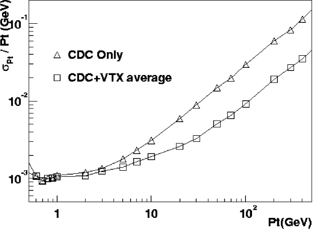
Figure 8.76: The $p_{t}$ resolution by a fit to CDC hits only and by a CDC and VTX helix average

Figure 8.77: The 2D impact parameter resolution as a function of $P_{t}$ by a fit to CDC hits only, VTX hits only and CDC-VTX helix average.

The impact parameter resolution as a function of $p_{t}$ is shown Fig. 8.77, which is about 25 $\mu$m at 1 GeV and about 3$\mu$m at high momentum.

The missing mass resolution was also studied using the process $e^{+}e^{-}\rightarrow\mu^{+}\mu^{-}X$. This is a channel to search the Higgs boson independently of its decay mode and the width of the Higgs boson can be measured if it is large enough. The beamstrahlung spectrum of JLC-I[17] X-band 300 GeV parameters with $\pm$0.5% initial energy spread was included in the simulation. The center-of-mass energy was 250 GeV.

The events were selected by requiring two good charged tracks (the number of sampling in CDC is equal to 50) with an invariant mass between 80 to 100 GeV. The obtained missing mass spectrum for an integrated luminosity of 100 fb^-1 is shown in Fig. 8.78. The spectrum was fitted by the curve given by

$$F(m)=N_{H}\int F_{H}(m,t)\exp^{-\frac{t^{2}}{2\sigma^{2}}}dt+N_{Z}\cdot F_{Z}(m),$$ (8.27)

where $F_{Z}(m)$ is the scaled missing energy with respect to $Z$( $F_{Z}(m)=1-\frac{m-M_{Z}}{\sqrt{s}-M_{Z}}$), and $F_{H}(m,t)$ is that to Higgs ($F_{H}(m,t)=Max(0,1-\frac{m-M_{H}+t}{\sqrt{s}-M_{H}})$).

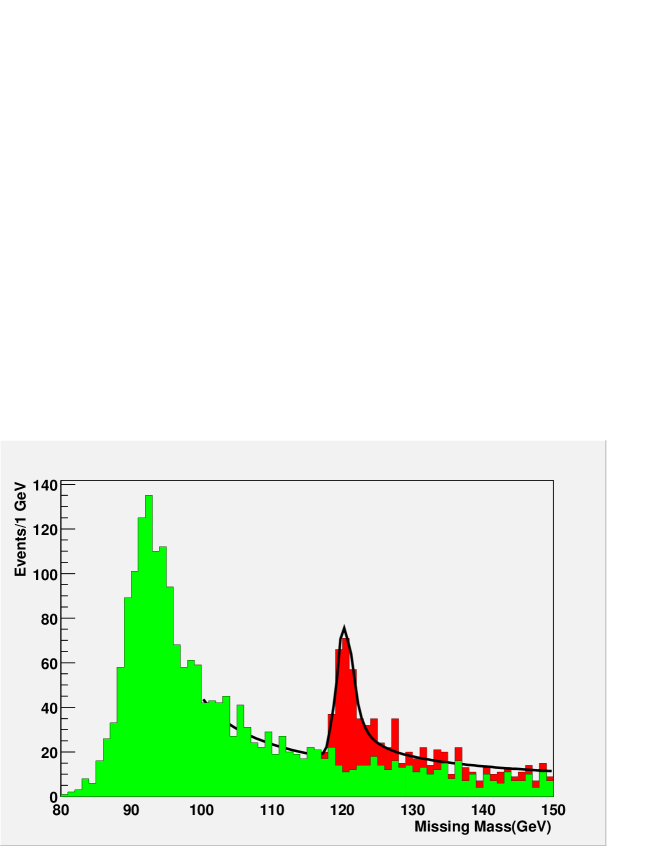
Figure 8.78: The missing mass spectrum of the two tracks for $e^{+}e^{-}\rightarrow ZH$(red) and $ZZ$(green) processes, where $Z$ decays to $\mu^{+}\mu^{-}$. The center of mass energy is 250 GeV, and the integrated luminosity is 100 fb^-1. The solid line is a fit by a function as described in the text.

From the fit, we obtained the missing mass resolution of 1.0 GeV. The main contribution to the width is the initial energy spread of $\pm 0.5\%$, but the resolution could be slightly improved to 0.9 GeV if the measurement is performed at 240 GeV.

Chapter 9 Calorimetry

9.1 Design Criteria

One of the most important physics to study at linear colliders is precision study of Higgs boson produced in a reaction $e^{+}e^{-}\rightarrow Z^{0}H$. Large backgrounds to this process from $W^{+}W^{-}$ and $Z^{0}Z^{0}$ pair productions should be removed by b-tagging and reconstructed 2-jet masses. Precision study of weak couplings and top properties also need precise event reconstruction using 2-jet masses under up to 8-jet environment. We therefore set a design criteria for the calorimeter system in combination with the central tracker such that the 2-jet mass resolution be as good as the natural width of weak bosons for excellent $W/Z$ identification. Based on this criteria, the baseline detector model has been made and simulation studies have been carried out.

In order to achieve the required 2-jet mass resolution, we set target energy resolution for calorimeters to be

$${\sigma_{E}\over E} = {15\%\over\sqrt{E{\rm(GeV)}}}\oplus 1\%~{}~{}~{}{\rm for~{}e/\gamma,~{}and}$$

$${\sigma_{E}\over E} = {40\%\over\sqrt{E{\rm(GeV)}}}\oplus 2\%~{}~{}~{}{\rm for~{}hadrons,}$$

with reasonably fine granularity. Here $\oplus$ means quadratic sum. In addition, the calorimeter should have cluster-position resolution better than 1 mm to achieve precise track-cluster association for precise energy reconstruction.

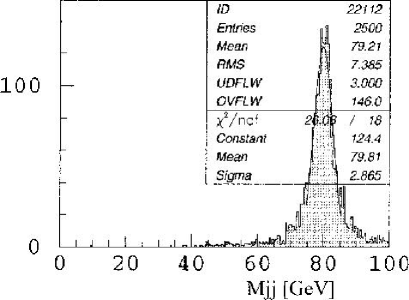
Figure 9.1: An example of reconstructed-mass resolution for $W$ with kinematical fit for the reaction $e^{+}e^{-}\rightarrow W^{+}W^{-}$ at $\sqrt{S}$ = 400 GeV, obtained by quick simulation with the baseline detector of 2Tesla version.

Fig.9.1 shows an example of 2-jet mass resolution obtained by quick simulation with the baseline detector of 2Tesla design for the reaction $e^{+}e^{-}\rightarrow W^{+}W^{-}$ at $\sqrt{S}$ = 400 GeV. Obtained mass resolution of 2.9 GeV with kinematical fit is reasonably good taking into account that analysis algorithm and parameters are not yet optimized very well. Various origins of the width are decomposed in the table 9.1. Each contribution was calculated by replacing each information with generator information.

Table 9.1: Various contributions to the width of reconstructed $W$ mass for the reaction $e^{+}e^{-}\rightarrow W^{+}W^{-}$ at $\sqrt{S}$ = 400 GeV.

Natural width of W	$\sim$ 1.6 GeV ( in terms of $\sigma$ )
Neutrino escape	$\sim$ 0.8 GeV
CDC momentum resolution	$\sim$ 1.3 GeV
CAL energy resolution	$\sim$ 1.2 GeV
Cluster-track association	$\sim$ 1.9 GeV
Jet clustering	$\sim$ 1.1 GeV
Total Width	$\sim$ 3.3 GeV ( without kinematical fit )

It has been widely known since the early days of $e^{+}e^{-}$ collider experiments that in order to achieve the best event reconstruction, tracking information should be used for charged particles, while calorimeter information should be used only for neutral particles. For this purpose, calorimeter hits generated by charged particles should be precisely identified and deleted. Therefore, excellent clustering followed by precise track-cluster association plays essential role in analysis. This conventional method has been used for analysis of quick-simulation data. Existence of neutral objects are identified solely by energy-momentum unbalance of associated cluster and track for overlapping clusters, which does not not require very fine granularity.

From the table, it is seen that more improvements in track-cluster association algorithm, and consequently in hadron clustering, should further improve this result. Needless to say, however, verification with full simulation is indispensable to validate/optimize the baseline parameters.

9.2 Baseline Design

The baseline calorimeter system is characterized by :

• excellent hadron energy resolution;

• reasonably fine granularity;

• whole calorimeter system inside of the superconducting solenoid.

Required hadron energy resolution of $40\%/\sqrt{E}$ can only be achieved with compensation, which means that calorimeter signals for EM particles and for hadrons of the same energy have the same amplitude. There are two ways to achieve the compensation; one is hardware compensation and the other is software compensation. Software compensation, first adopted by H1 $liq.$Ar calorimeter [1], requires very fine granularity to apply to linear collider detectors aimed at precision physics, and thus results in very high cost. On the other hand, hardware compensation can be achieved by simply adjusting the calorimeter composition, and requires no additional effort/cost. We therefore chose hardware-compensation with tile/fiber technique as the baseline design. By adopting hardware compensation, we can de-couple energy resolution and granularity ; the best energy resolution can be achieved regardless the granularity, and granularity can be determined only by the criteria from topological reconstruction.

The tile/fiber technique, which will be described in detail in the following sections, has following features:

• Essentially crack less hermeticity;

• Capability for very fine longitudinal segmentation;

• Easy to design projective tower layout;

• Easy to integrate pre-shower and shower-max detectors;

• Reasonable transverse segmentation;

• Less expensive than crystals and liq.Ar.

In addition, the hardware compensation results in following features:

• Excellent hadron energy resolution and linearity;

• High density;

• Reasonable EM energy resolution;

• Relatively low light yield.

Our analysis based on quick simulations indicates that very fine granularity is not necessary for event reconstruction. Therefore present baseline design is considered to be almost optimum for the hadron calorimeter (HCAL). For the EM calorimeter (EMC), on the other hand, very fine granularity might be required for precise event topology reconstruction, even though quick simulation tells us that present granularity shows high performance. In that case software compensation would be another option. Further simulation analysis will answer this question.

We also need excellent pre-shower detector (PSD) and shower-max detector (SMD) for $e/\gamma/\pi^{\pm}/\pi^{0}$ separation, two-cluster identification, and track-cluster association. To have plural layers of shower position detectors (SPD) in EMC enables precise measurement of off-vertex photon direction.

All the calorimeter system, including the photon detectors, are designed to be located inside of the 3Tesla (or 2Tesla) magnetic field. We therefore need high-gain high-sensitivity photon detectors operational in the strong magnetic field, since hardware compensation results in relatively poor photon yield compared to the usual sampling calorimeters. We discuss such photon detectors in a separate section.

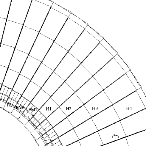
Figure 9.2: Configuration of the baseline design of barrel calorimeter system (x-y cross section) implemented into a full simulator.

The GEANT3 drawing of the baseline-design barrel calorimeter is shown in Fig.9.2. There are 2Tesla option and 3Tesla option. Sizes of the calorimeter are smaller for the latter, but configuration is almost the same.

In the case of the 3Tesla design, inner and outer radii of the barrel calorimeter are 160 cm and 340 cm, respectively, and the length is $\pm$180 cm. Inner radius of the endcap calorimeter is 50 cm, and the front face locates at $z=\pm 190$ cm. Angular coverage of the endcap calorimeter with full-thickness therefore extends to $\mid$cos$\theta\mid<0.966$, while partial-thickness coverage extends to $\mid$cos$\theta\mid<0.991$.

The calorimeter is an array of super-towers with pointing geometry with small offset. One super-tower is composed, from the inner-radius to the outer-radius, of PSD (3$\times$3 in a super-tower), SMD, EMC-1(3$\times$3), SPD, EMC-2(3$\times$3), HCAL-1, HCAL-2, HCAL-3, and HCAL-4. There are about 2000 super-towers in the barrel calorimeter, and about 3000 in total in the endcap calorimeters. One super-tower has readout channels of 31 and 48 for calorimetric measurement and for position measurement, respectively.

Parameters of these sub-detectors are summarized in Table 9.2. All the parameters in the table are the first trials, and optimization with full simulation is needed.

Table 9.2: Parameters of the calorimeter system implemented into a full simulator. 2Tesla option is a revision of the previous large detector option, and 3Tesla option is a new detector design.

9.2.1 EM Calorimeter (EMC)

EMC is a sampling calorimeter composed of 4mm-thick lead plates and 1mm-thick plastic scintillator plates. Photons from the scintillator plates (tiles) are read out via wavelength shifting fibers (WLS fibers) embedded in the tiles. Each WLS fiber is connected to a clear fiber at the exit of the tile, and photons are transfered through the clear fibers to photon detectors (tile/fiber technique). There are several ways to layout the clear fibers. Here we adopted CDF-type[2] ; additional 1mm-thick acryl plates are stacked on the tile assembly to accommodate clear fibers. This sampling frequency is expected to achieve stochastic term of the EM energy resolution of 15$\%/\sqrt{E}$, provided that photon statistics does not contribute.

EMC is longitudinally divided into PSD, EMC1 and EMC2, to improve hadron/electron identification. Thicknesses of these sections are 4.3 $X_{0}$ (radiation length), 8.6 $X_{0}$, and 14.3 $X_{0}$, respectively. We expect pion rejection better than 1/1000 with electron efficiency of 98% when used with HCAL information. Transverse cell size of EMC is 4cm$\times$4cm in the baseline design of 3Tesla-version, and 3$\times$3 EMC cells cover one HCAL cell. This transverse size is limited by the cost and technical feasibility of small tiles, or to be more precise, bending radius of WLS fibers at corners.

9.2.2 Hadron Calorimeter (HCAL)

HCAL is composed of 8mm-thick lead plates, 2mm-thick plastic scintillator plates, and 2mm-thick fiber-routing acryl plates. HCAL also has tile/fiber configuration. This sampling frequency was expected to achieve stochastic term of the hadron energy resolution of 40$\%/\sqrt{E}$, provided that photon statistics did not contribute.

HCAL is longitudinally divided into four sections with thicknesses of 1.25 $\lambda_{0}$ (interaction length), 1.5 $\lambda_{0}$, 1.75 $\lambda_{0}$, and 2.0 $\lambda_{0}$. Total thickness including EMC is 7.5 $\lambda_{0}$. Transverse segment size of HCAL is 72 mrad at $\theta=90^{\circ}$ seen from the interaction point, which corresponds to 14cm at the front face of HCAL section in the case of 3Tesla-design.

Number of longitudinal segmentation is limited only by number of photon-detector channels. Improvement in multi-channel photon detectors enables much finer longitudinal segmentation, and thus enables more sophisticated clustering and two-cluster separation algorithms. Transverse segment size, on the other hand, is limited by cost, and it seems difficult to make it much smaller.

9.2.3 Shower-Max Detector(SMD) and Shower-Position Detector(SPD)

The purpose of SMD is $\pi^{0}/\gamma$ identification, precise measurement of cluster position for track-cluster association, and two-cluster recognition. SMD also improves $e/\pi^{\pm}$ separation by transverse signal distribution. For this purpose, fine segmentation is necessary for SMD. Also needed is wide dynamic range to detect minimum-ionizing particles (MIP) and developing EM showers simultaneously.

The baseline design for SMD is an arrays of plastic scintillator strips. Strip size of 1cm-wide and 5mm-thick is assumed at present. An array of 12 strips covers one super-tower in the case of 3Tesla design, and 18 strips in the case of 2Tesla design. Two orthogonal layers give $\theta-\varphi$ position information with accuracy of better than 1 mm for $e/\gamma$ of energy greater than a few GeV. Ghosts are removed, though not completely, by pulse-height analysis.

In the baseline design, photons from the scintillator strips are read out by WLS-fibers, similar to the tile/fiber technique. Another option is under study to read out photons using photo-diodes directly attached on the strips.

Another shower position detector (SPD) is installed between EMC-1 and EMC-2. SPD has the same configuration as SMD. The purpose of SPD is to measure the direction of the isolated off-vertex photons. SPD also helps hadron shower position measurement by measuring early stage of hadron shower development, and thus improves track-cluster association for charged hadrons.

The baseline design has only one set of SPD. Whether we need more layers or not should be investigated.

9.2.4 Photon Detectors

Photon detectors for scintillating light are designed to sit at the end of the calorimeter assembly in the magnetic field, rather than stretching the clear fibers to the outside of the iron yoke of the whole detector. Therefore high-sensitivity photon detectors operational inside of 3Tesla (or 2Tesla) magnetic field are necessary. At present, we assume that;

• Both EMC and HCAL are read out by multi-channel HPDs;

• PSD are read out either by multi-channel HPDs or multi-channel HAPDs;

• SMD and SPD are read out either by multi-channel HAPDs or EBCCDs.

Here HPD, HAPD and EBCCD stand for Hybrid Photo-Diode, Hybrid Avalanche Photo-Diode, and Electron-Bombarded CCD, respectively. Though some fine-mesh photo-multiplier tubes show quite high gain even in 2.5 Tesla, we decided not to use them. Detailed R&Ds are further needed to decide which option is the optimum.

There are 125k , 19k, and 223k channels of EMC, HCAL, and SMD/PSD to read out, respectively. Therefore, it is impractical to use single-channel photon detectors. With multi-channel HPDs and EBCCDs under study at present, only one multi-channel HPD and one EBCCD can read out of all the calorimetric signals and position detector signals from one super-tower, respectively.

9.2.5 Other Detector Options

There are several calorimeter schemes other than the baseline-design tile/fiber scheme. The features of various detector schemes are summarized in Table 9.3. The listed features are just potentials, and whether constructed detectors really have such features or not is a different question. For the energy resolution, resolutions of typical EM calorimeters are quoted. Hadron energy resolution strongly depends on the detailed structure and analysis algorithm, and thus is not quoted. It should be stressed that longitudinal segmentation is essentially important for $e/\pi$ separation.

Table 9.3: Properties of various detector schemes for EM calorimetry.

Detector Scheme	Crystal	SPACAL	Shashlik	W/Si	Liq/Ar	Tile/Fiber
EM Energy Resolution	Excellent	Good	Good	Good	Good	Reasonable
Transverse Segmentation	Good	Good	Good	Excellent	Excellent	Reasonable
Longitudinal Segmentation	Poor	Poor	Poor	Excellent	Excellent	Excellent
Hermeticity	Good	Good	Good	Excellent	Reasonable	Excellent
Cost	Expensive	Expensive	Expensive	Very Expensive	Expensive	Reasonable
Examples	L3, Belle CMS	H1, KLOE	Phenix, Hera-B	Luminosity monitors	SLD, D0, H1, ATLAS	CDF, STAR

Besides the properties in the table, cryo-liquid calorimeters have additional features inadequate for precision physics such as:

• Cryogenic pipes and walls tend to behave as anomaly (or a hole at the worst case);

• Materials and gap between inside tracker and EMC deteriorate track-cluster association and EMC performance.

Nevertheless, $liq$.Ar calorimeter has been adopted by ATLAS EMC due to its high resistance against radiation damage, which is not the case for linear collider environment. For large-scale general-purpose detectors at linear colliders, therefore, tile/fiber scheme has the best-balanced features.

9.3 Hardware Study

9.3.1 ZEUS-type Test Module

We first investigated the possibility of ZEUS-type sandwich calorimeter because it was the best-operating hadron calorimeter in the collider detectors when we started R&Ds. We built four hadron calorimeter test modules with similar configuration to the ZEUS test modules[3]. It was composed of 10mm-thick lead plates and 2.5mm-thick plastic scintillator plates as shown in Fig.9.3. This volume ratio was expected to achieve hardware compensation. Photons were read out by WLS plates attached on the both sides of the stack. Photon collection efficiency was higher than the tile/fiber scheme. Number of layers was 80, which corresponds to the total thickness of 5$\lambda_{0}$. This simple structure realizes low-cost and easy assembling, but at the same time results in a massless gap between modules.

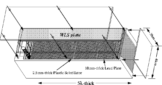
Figure 9.3: Schematical drawing of ZEUS-type test module.

     

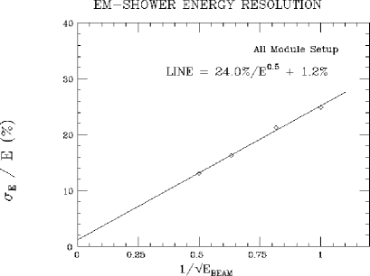
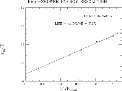
Figure 9.4: Energy resolutions of ZEUS-type hadron calorimeter test modules for electrons (left) and for pions (right).

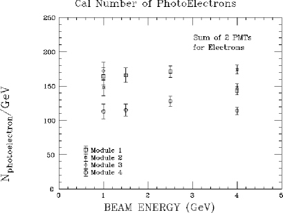
Figure 9.5: Photo-electron yield of ZEUS-type hadron calorimeter test modules for electrons. The same amount is expected for pions since the module was hardware-compensating.

A test beam measurement was carried out at KEK $\pi$2 beamline[4] using 1-4 GeV beams with a PSD, an SMD, and a SPACAL-type test module, which is described in the next section. Measured energy resolution is shown in Fig.9.4. The results were as expected except the large constant term for pions, which was due to transverse shower leakage caused by small detector assembly cross section of 60cm$\times$60cm. An e/$\pi$ ratio, a measure of compensation, was obtained to be 1.01. Also obtained was photo-electron yield of the module to be 160 p.e./GeV on average as shown in Fig.9.5. This photo-statistics worsens the pion energy resolution from 40.0%/$\sqrt{E}$ to 40.8%/$\sqrt{E}$. This is not a problem for hadron calorimetry.

     

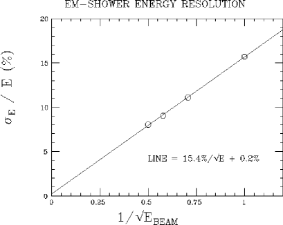
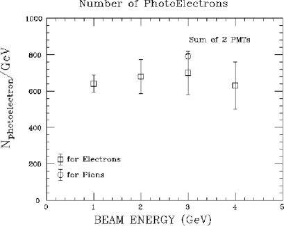
Figure 9.6: Energy resolution (left) and photo-electron yield (right) of ZEUS-type EM test module.

In order to test the response to electrons, another ZEUS-type EM calorimeter test module was made with 4mm-thick lead plates and 1mm-thick plastic scintillator plates. Beam test was carried out at KEK $\pi$2 beamline with 1-4 GeV beams. Measured energy resolution and photo-electron yield are shown in Fig.9.6. Obtained energy resolution of $15.4\%/\sqrt{E}+0.2\%$ satisfies expected resolution. The measured photo-electron yield of 660 p.e./GeV has effect on the stochastic term of the energy resolution to worsen it from 15.0%/$\sqrt{E}$ to 15.5%/$\sqrt{E}$. Though this would be acceptable, photon readout scheme with better photon collection efficiency might be preferred for EMC.

Though measured energy resolutions were quite satisfactory, we decided not to continue R&Ds of ZEUS-type sandwich calorimeter due to following reasons:

• Longitudinal segmentation is difficult;

• Massless gap made by WLS plates running radially introduces significant response anomaly.

9.3.2 SPACAL-type Test Module

  

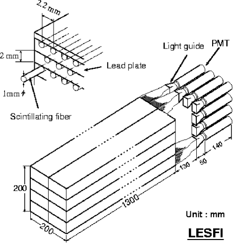
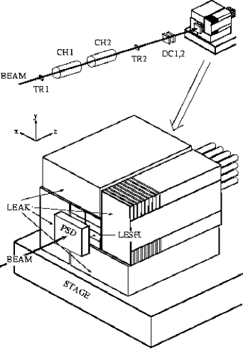
Figure 9.7: Schematical drawing of the SPACAL-type test module (left) and setup of the combined beam test of ZEUS-type and SPACAL-type test modules at KEK-$\pi 2$ beamline (right).

     

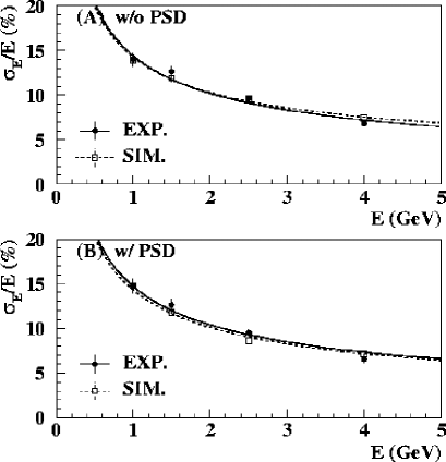
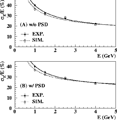
Figure 9.8: Energy resolutions of SPACAL-type test module for electrons (left) and for pions (right). Bottom figures are for measurements with PSD in front, and top ones are without PSD. Dotted lines are results of GEANT simulation.

We studied SPACAL-type calorimeter in parallel with the ZEUS-type calorimeter at the first stage of the R&D because the SPACAL-type calorimeter was the best-performance calorimeter that time, even though there was no running experiment using SPACAL. Since SPACAL-type calorimeter was quite expensive and extremely elaborating, we built only one module with sizes of 20cm$\times$20cm$\times$130cm as shown in Fig.9.7. Pure lead plates with grooves were stacked, and 1 mm$\phi$ scintillating fibers were embedded in the grooves. The volume ratio of lead to scintillator was 4:1 for hardware compensation. One module was read out by 16 PMTs to have $4\times 4$ sub-tower structure for transverse shower profile measurement.

Beam test was done at KEK $\pi$2 beamline using 1-4 GeV beams[4]. The setup is also shown schematically in Fig.9.7. One SPACAL-type module at the center was surrounded by four ZEUS-type calorimeter modules, and a PSD was set in front of the SPACAL module for several measurements.

Measured energy resolutions are shown in Fig.9.8. The results are parametrized as

$${\sigma_{E}\over E} = {(14.4\pm 0.3)~{}\%\over\sqrt{E{\rm(GeV)}}}\oplus(0.0\pm 1.4)~{}\%~{}~{}~{}{\rm for~{}electrons,}$$

$${\sigma_{E}\over E} = {(38.1\pm 1.3)~{}\%\over\sqrt{E{\rm(GeV)}}}\oplus(11.6\pm 1.4)~{}\%~{}~{}{\rm for~{}pions.}$$

These resolutions were very good except the large constant term due to transverse shower leakage. We also obtained pion rejection factor of 1/200 with electron efficiency of 98% using PSD pulse height and transverse shower profile. This rejection score is not very high because it is difficult to separate $e/\pi$ with transverse shower profile at low energies.

In conclusion of the series of R&Ds, we decided not to continue R&Ds of SPACAL-type calorimeter due to following reasons:

• Longitudinal segmentation is very difficult;

• Pre-shower and shower-max detectors can not be integrated naturally;

• Really expensive and elaborating.

9.3.3 Tile/Fiber Test Module

Tile/fiber structure is characterized by a wavelength shifting fiber embedded in a plastic scintillator tile. This enables compact optics for light collection and transfer from scintillators to photon detectors without sacrificing photon yield so much. This scheme was extensively studied by SDC group[5], and then by CDF group[2] with slightly different fiber layout. The tile/fiber calorimeters have been widely adopted by CDF, STAR[6], CMS[7], and so on. For the JLC calorimeter, the tile/fiber structure with hardware compensation was adopted as a revised baseline design in 1996, and systematic R&Ds were initiated. Following bench tests of each component, test modules were constructed for generic shower study and realistic performance study, and series of beam tests were carried out at KEK and at FNAL. In the following sections, detail of the R&Ds are described.

     

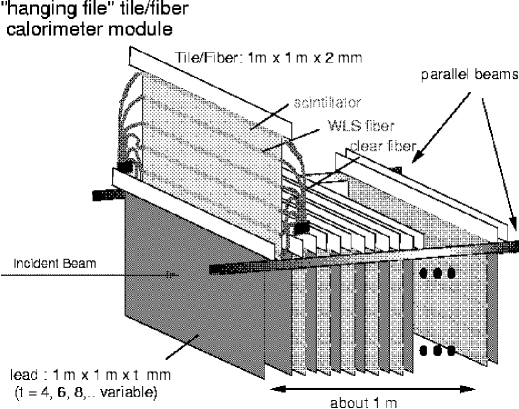
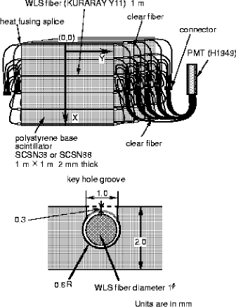
Figure 9.9: Schematical view of straight-groove hanging-file test module (left), and optical readout scheme (right).

1) Generic Studies with Straight-groove Module

Though extensive R&Ds had been carried out by SDC/CDF group before 1996, combination with hardware compensation raised two open questions:

• Possibility of hardware compensation itself with tile/fiber configuration must have been established. There were several calculations and measurements on compensation with lead and plastic scintillator sampling calorimeters[4, 8, 9]. However those results had significant discrepancies with each other. Addition of fiber-routing plates for tile/fiber configuration was another unknown factor on compensation. This might affect the compensation condition. Those problems must have been examined before making calorimeter module of tile/fiber design.

• In order to realize required energy resolution with hardware-compensating composition using lead absorber, very thin scintillator plates of 1mm-thickness should be used for EM calorimeter, and 2mm for hadron calorimeter. Photon yield, uniformity, and mechanical feasibility must have been examined for such thin scintillator plates.

A test module with hanging-file structure was constructed to examine possibility of hardware compensation. The structure is schematically shown in Fig.9.9. Lead plates and scintillator plates, and acryl plates if necessary, were hung over a pair of supporting beams to enable re-configuration for generic studies. As absorbers, 4mm-thick lead plates and 2mm-thick lead sheets were used to change the lead thickness from 4 mm to 16 mm by 2mm-step. The thicknesses of plastic scintillator plates and acryl plates, on the other hand, were fixed to be 2 mm. Transverse size of the plates were 1m$\times$1m for good shower containment.

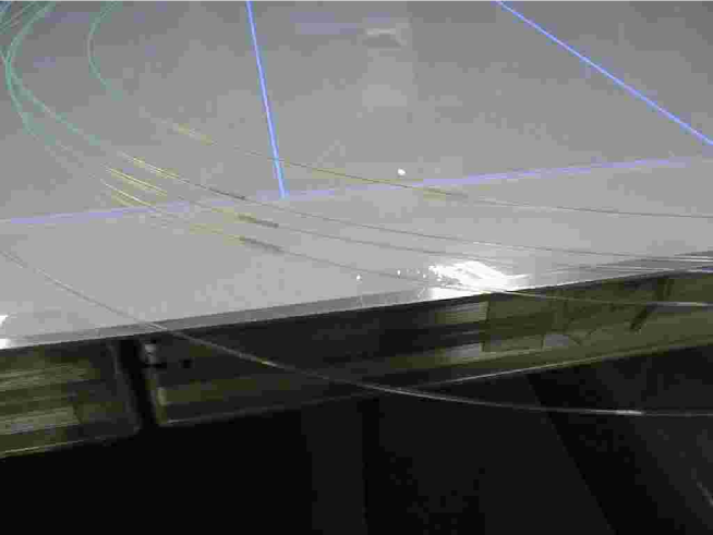
Figure 9.10: A scintillator plate with WLS fibers. Blue lines on the scintillator are the grooves. Green part of the fibers are WLS fibers to be embedded in the grooves. A clear fiber is connected to each WLS fiber by heat-fusing with a protective sleeve.

Photon-readout scheme is shown in Fig.9.9 and in Fig.9.10. The scintillator plates had six straight grooves of key-hole cross section, where 1 mm$\phi$ WLS fibers were embedded. Distance between the grooves, 20cm, was determined to re-use the scintillator plates for the tile/fiber module. Fibers from five successive scintillator plates on each side were ganged to form a super layer, and were read out by one PMT. There were 42 super layers in the configuration with 4mm-thick lead plates, and detailed study on longitudinal shower profile was carried out. In the case of 8mm-thick lead plates, there were 24 super layers, resulting in the total thickness of 6$\lambda_{0}$.

     

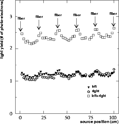
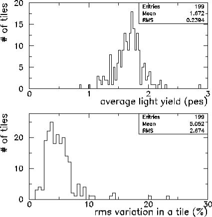
Figure 9.11: Non-uniformity of photo-electron yield over one scintillator plate (left), distributions of its average (right-top) and RMS (right-bottom) for 199 plates.

Response of scintillator plates were measured with an RI source before assembling. Non-uniformity of photo-electron yield over one scintillator plate and distributions of its average and RMS for 199 plates are shown in Fig.9.11. Since the WLS-fiber distance is rather large, average photo-electron yield is only 1.6 p.e./MIP. Measured response map shows prominent peaks at the embedded WLS locations. Effects of both measured non-uniformity and distribution of average photo-electron yield on calorimeter responses were examined by GEANT simulation, and concluded not to be significant for hadrons[10].

Energy Measurement

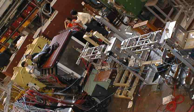
Figure 9.12: Setup of the beam test of hadron calorimeter test module at KEK.

Series of beam tests were carried out at KEK $\pi$2 beamline with beam energies from 1 GeV to 4 GeV[10]. The setup of the beam test is shown in Fig.9.12. Fig.9.13 shows energy resolution for pions and e/$\pi$ response ratio versus lead plate thickness. Target energy resolution is achieved with lead plates of 8mm-thick or thinner. The hadron energy resolution of 33.6%/$\sqrt{E}$ achieved with 4mm-thick lead plates are one of the best hadron energy resolution achieved so far. In Fig.9.13, dependence of energy resolution on lead thickness $d$ is parametrized as $\sigma_{E}=\sqrt{\sigma_{intrinsic}^{2}+(\sigma_{sampling}^{2}+\sigma_{photostat}^{2})/d}$, neglecting the constant term. Intrinsic hadron shower fluctuation was obtained to be 24.4$\pm$0.7% as a result of the fitting. This is significantly larger than previously reported value of 13.4$\pm$4.7% by ZEUS [11], which was derived only from two sampling frequencies. However this could simply be due to the difference of incident energy.

It is concluded from the fitting of $e/\pi$ ratio in Fig.9.13 that hardware compensation should be achieved with 9mm-thick lead plates in the case of 2mm-thick plastic scintillator plates.

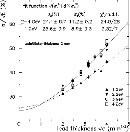
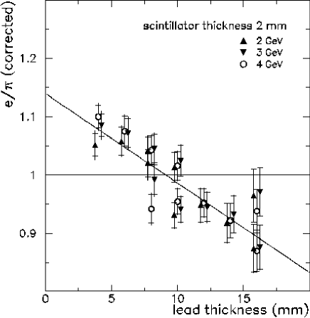
Figure 9.13: Energy resolution for pions (left) and e/$\pi$ ratio (right).

In order to check effect of fiber-routing acryl plates on compensation, three configurations are tested in the case of 8mm-thick and 16mm-thick lead plate configurations:

• no acryl plates were used (lead and scintillator only);

• an acryl plate was put upstream-side of every scintillator plate;

• an acryl plate was put downstream-side of every scintillator plate.

The motivation of measurement with 16mm-thick lead plates was such that compensation might be achieved with 16mm-thick lead plates + 2mm-thick scintillator plates + 2mm-thick acryl plates, resulting in the volume ratio of lead to total plastic to be 4:1.

Effects of acryl plates on the energy resolution and e/$\pi$ ratio is summarized in Table 9.4. It is seen from the results of 8mm-thick lead-plate case that acryl plates does not destroy the hardware compensation if they are placed downstream-side of scintillator plates. Hadron energy resolution, however, gets slightly worse by their presence regardless of their location. These behaviour is not clear in the case of 16mm-thick lead-plate case due to large error. However it is clear that compensation was not achieved, meaning that acryl plates do not contribute to the volume-ratio counting.

Table 9.4: Energy resolutions and $e/\pi$ ratios with and without acryl plates for 4 GeV/c electrons and pions.

lead thickness	position of acryl	$\sigma_{E}/E$ for electrons	$\sigma_{E}/E$ for pions	$e/\pi$ ratio
8mm	No acryl plates	(12.0$\pm$0.5)%	(20.5$\pm$0.4)%	1.03$\pm$0.02
	Acryl plates upstream	(11.6$\pm$0.5)%	(22.7$\pm$0.4)%	1.07$\pm$0.02
	Acryl plates downstream	(12.0$\pm$0.5)%	(22.8$\pm$0.4)%	1.01$\pm$0.02
16mm	No acryl plates	(18.1$\pm$1.1)%	(27.1$\pm$0.7)%	0.90$\pm$0.04
	Acryl plates upstream	(18.1$\pm$1.1)%	(28.1$\pm$0.7)%	0.95$\pm$0.04
	Acryl plates downstream	(18.1$\pm$1.1)%	(28.8$\pm$0.7)%	0.87$\pm$0.04

Shower Fluctuation Analysis

     

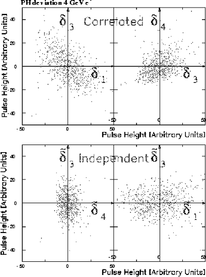
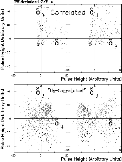
Figure 9.14: Correlation between pulseheight fluctuations for different super layers for electrons (left) and for pions (right). Upper distributions are for raw fluctuations, and lower ones are after orthogonalization.

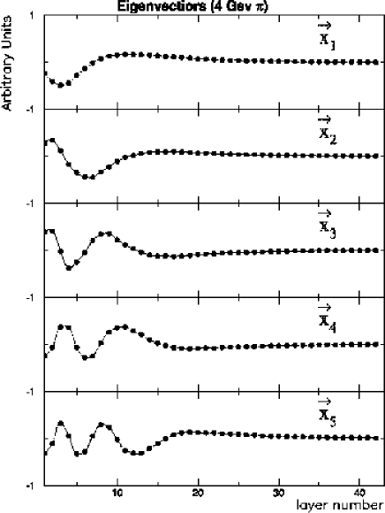
Figure 9.15: Shape of the orthogonalized fluctuation mode (eigen vectors) for 4 GeV pion shower. Five major modes are shown. Horizontal axis is super layer number, and vertical axis is amplitude of deviation (arbitrary unit).

Longitudinal shower profile and its event-by-event fluctuation have been studied with configuration of 4mm-thick lead plates, which had 42 longitudinal samplings (super layers). The purposes of this study are;

• Improve hadron energy resolution (software weighting);

• Construct parametric hadron shower generator with realistic fluctuation;

• Obtain $e/\pi$ separation capability as a function of the longitudinal segmentation of the calorimeter.

Analysis has been done for both EM and hadron showers following the work by CDF for EM shower analysis[12]. Correlation between pulseheight fluctuations for different super layers are shown in Fig.9.14. Upper plots are for raw fluctuations $\delta_{i}$ from average shower shape, where $i$ means $i$-th super layer.

Orthogonalization is done by diagonalizing correlation matrix

$$C_{ij}=\frac{1}{N}\sum_{k}\delta_{i}^{k}\delta_{j}^{k}$$

where $k$ means $k$-th events. As the eigen vectors and eigen values of the diagonalized matrix, we obtain orthogonalized fluctuation modes and their amplitude $\tilde{\delta}$, respectively. Fig.9.15 shows five major eigen vectors (orthogonalized fluctuation modes) for 4GeV pion shower. Horizontal axis is super layer number. Lower plots in Fig.9.14 are correlation between fluctuation of amplitudes $\tilde{\delta_{i}}$ and $\tilde{\delta_{j}}$ for $i$-th and $j$-th orthogonalized fluctuation mode. In the case of electrons (left), no correlation is seen between amplitudes of the orthogonalized eigen vectors. On the other hand, $\tilde{\delta_{i}}$ for pions (right) have correlation even after orthogonalization procedure, meaning that orthogonalization of hadronic fluctuation is not yet successful. This is because hadronic fluctuation is not Gaussian due to its two-component nature; global hadronic fluctuation and local $\pi^{0}$ generation. An attempt has been under study to decompose two fluctuations. Therefore parameterization of hadron shower fluctuations with orthogonal parameter set has not been completed yet.

     

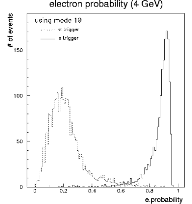
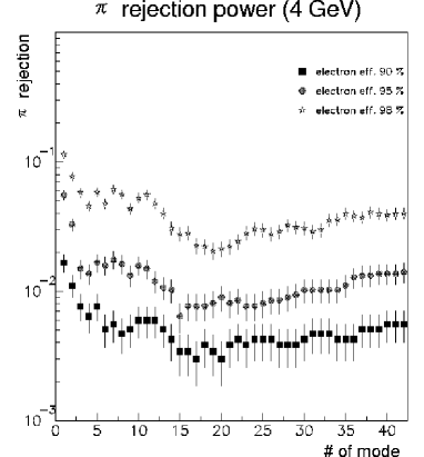
Figure 9.16: $e/\pi$ separation by deviation of pulseheight fluctuation from template fluctuation distributions for electrons and pions. Left histogram is electron probability distribution for electron and pion samples, and right plot is pion rejection factor as a function of number of modes (used eigen vectors).

Pulseheight fluctuation can be used to improve $e/\pi$ identification, which is usually done by shower profile only. Deviations of measured pulseheights from electron profile template and from pion profile template are normalized by typical fluctuation for each particle, and likelihood to each particle are calculated. Distribution of electron-ness and pion rejection capability are shown in Fig.9.16. Number of mode in the right figure is number of eigen vectors of pulseheight fluctuation used in the analysis. Since there are 42 super layers, there are 42 orthogonal eigen vectors to represent pulseheight fluctuation. Using six or seven major eigen vectors achieves almost the best score ; higher minor eigen vectors are noisy, and using them does not improve the score. For single-particle $e/\pi$ separation, therefore, six or seven longitudinal segmentation should be good enough if they are segmented in optimum way.

2) Study of Tile/Fiber Module

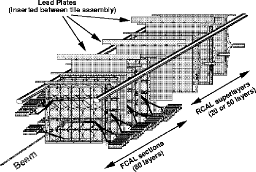
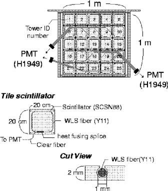
Figure 9.17: Schematic view of the tile/fiber test module (left) and layout of fibers and tiles (right).

Based on the results of the generic studies and tile bench tests, the straight-groove module was rebuilt to be a tile/fiber calorimeter module. The design of the module is schematically shown in Fig.9.17. The module was composed of a front section (FCAL) and a rear section (RCAL).

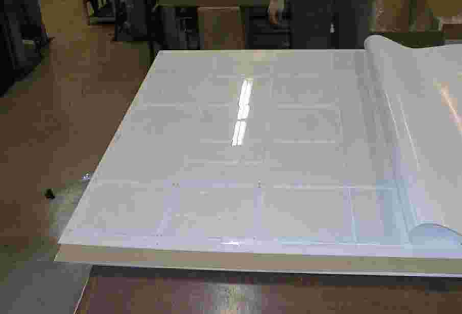
Figure 9.18: Scintillator tiles arranged as $5\times 5$ on the fiber-routing plate, and covered with white PET films.

In the FCAL part, the 1m$\times$1m plastic scintillator plate was modified to be a scintillator tile assembly as shown in Fig.9.17. Twenty-five tiles with size of 20cm$\times$20cm$\times$2mm-thick were arranged on a fiber-routing acryl plate to form 5$\times$5 tower structure. Four sides of the tiles were painted white with TiO₂-based emulsion, and the assembly was covered with white PET films for better light collection efficiency as shown in Fig.9.18. The tile had a $\sigma$-shaped groove with a key-hole cross section, where a WLS fiber was embedded. The WLS fiber was connected to a clear fiber by heat splicing at the exit from the tile. The clear fiber then ran in the groove on the fiber-routing acryl plate to exit from the detector assembly, and was connected to a photon detector.

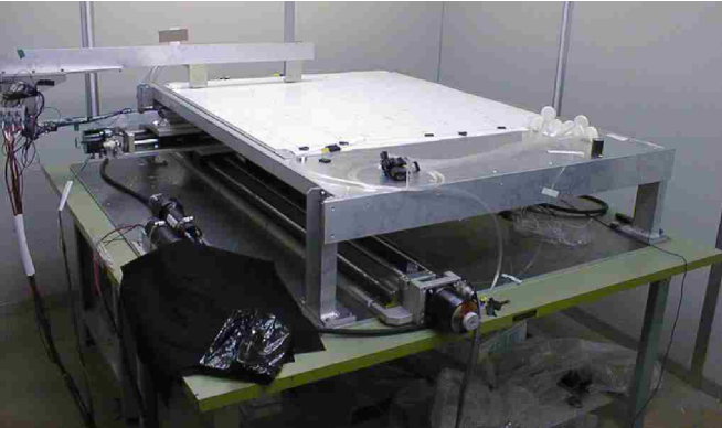
Figure 9.19: Automatic measurement stage for photo-electron yield uniformity.

Prior to assembling to 5$\times$5 matrix, photo-electron yield uniformity over a tile were measured with $\beta$ rays from an RI source for several tiles. Then after assembling to $5\times 5$ matrix, photo-electron yield at the center of each tile was measured for all 2000 tiles. The setup of the measurement system is shown in Fig.9.19, and the results are shown in Fig.9.20. Obtained photo-electron yield is translated to the calorimeter response of 83 p.e./GeV for 8:2 configuration, about the half of the ZEUS-type modules. This slightly worsens the stochastic term of hadron energy resolution from 40%/$\sqrt{E}$ to 41%/$\sqrt{E}$, which is not a problem for hadron calorimetry. The measured non-uniformity was estimated using GEANT3 simulation to introduce systematic uncertainty of 0.3% on average on energy resolution measurement. This, again, is not significant.

     

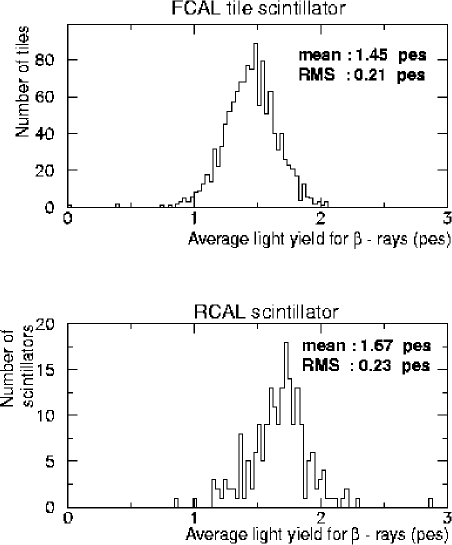
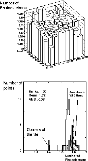
Figure 9.20: Average photo-electron yield for tiles (left-top), average photo-electron yield for straight-groove plates (left-bottom), uniformity over one tile (right-top), and distribution of photo-electron yield for 100 sampling points over one tile (right-bottom).

     

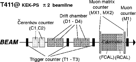
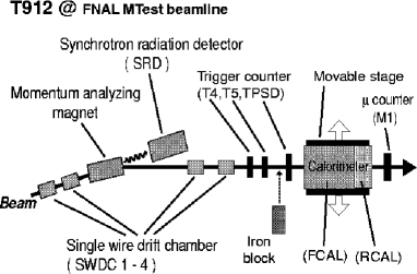
Figure 9.21: Setup of the beam test at KEK (left) and at FNAL (right).

These tile assemblies were interleaved with 8mm-thick lead plates. There were 80 layers of the tile assemblies in FCAL in total. They were divided into four sections longitudinally, each of which contained 20 layers. One quadrant of a tower was read out by one PMT.

Following the tile/fiber part, unmodified straight-groove section remained as RCAL. There were two super layers in RCAL in the case of low energy beam test at KEK. In the case of high energy beam test at FNAL, ten super layers were installed, the last of which did not have lead absorbers to be used for muon tagging. RCAL also had 8mm-thick lead plates as absorber.

The layouts of the beam tests at KEK and at FNAL are schematically shown in Fig.9.21. Both setups are quite similar except for that there were momentum-analyzing devices at FNAL beam test, and that SRD was used for electron identification at FNAL instead of Cherenkov counters. Details of the setup and analysis are given elsewhere[10, 13]. Energy of the beam was 1-4 GeV and 10-200 GeV at KEK and at FNAL, respectively. The beam was unseparated, and particle identification was done off-line. In the case of FNAL test, however, electron-rich and pion-rich conditions were realized by selecting appropriate converters/absorbers on the beamline. Tower-to-tower gain calibration was done using penetrating muons.

Energy Measurement

     

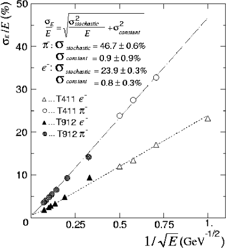
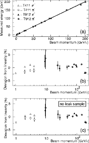
Figure 9.22: Energy resolution (left) and linearity (right) of the tile/fiber test module.

Measured energy resolution, linearity, and $e/\pi$ ratio are shown in Figs.9.22 and 9.23. The energy resolution is slightly worse than those shown in Fig.9.13, and is consistent with that of the straight-groove module with acryl plates interleaved shown in the Table 9.4. We can therefore conclude that acryl plates used for fiber-routing do deteriorate the energy resolution, regardless their location. On the other hand, the $e/\pi$ ratio is consistent with 1.0, and hardware compensation is established to be retained in the case of the tile/fiber structure if each acryl plate is located downstream-side of each scintillator assembly.

If we stick to the hadron energy resolution of 40%/$\sqrt{E}$, sampling frequency of the HCAL should be finer than 8mm-thick lead plates plus 2mm-thick plastic scintillator. However measured hadron energy resolution of 46%/$\sqrt{E}$ may be acceptable for physics analysis. This should be examined by further simulation study.

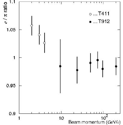
Figure 9.23: e/$\pi$ response ratio of the tile/fiber test module. T411 and T912 denote beam test at KEK and at FNAL, respectively.

Tower Property

Cross-talk between towers measured with electron central injection are shown in Fig.9.24. Amount of cross talk to adjacent towers are 1%-level. This is consistent with the optical crosstalk at the bench test measured with an RI-source. Cross talk of this level is negligible to hadron shower analysis. For EMC of finer-granularity option, however, cross talk may have significant impact, and needs to be examined.

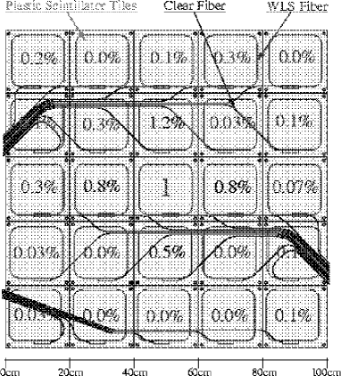
Figure 9.24: Cross talk between towers for the tile/fiber test module.

Response at the tower boundary are shown in Fig.9.25. Energy measurement for pions may have enhancement of about 3% at the region where WLS fibers are embedded. This is consistent with the non-uniformity at the bench test shown in Fig.9.20. This enhancement is not significant when EMC is located before the HCAL and response smears out. On the other hand, energy measurement for electrons has prominent enhancement at the boundary. This must be equalized by adjusting reflection index of tile surface around the WLS when EM modules are constructed.

         

         

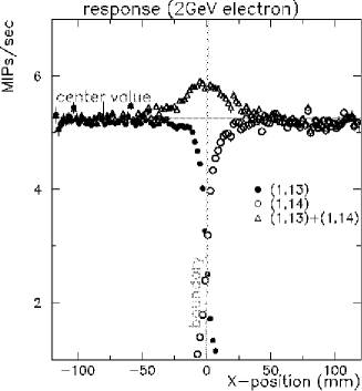
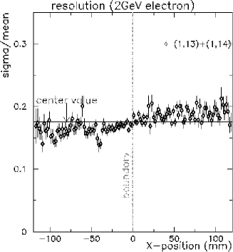
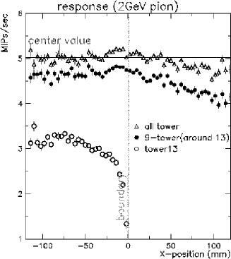
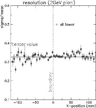
Figure 9.25: Tower boundary response of the tile/fiber test module. Top figures are responses for electrons, and bottom ones are for pions. Left figures are energy measurement, while right ones are energy resolutions.

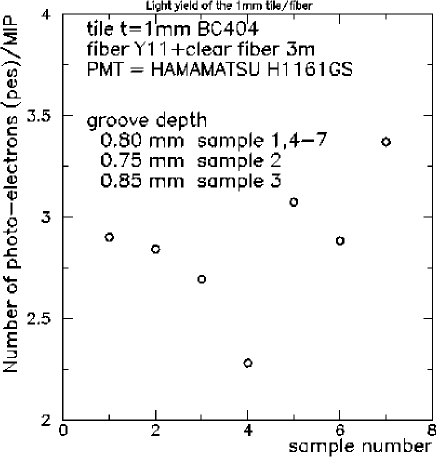
Figure 9.26: Photo-electron yield of 10cm$\times$10cm$\times$1mm-thick tiles.

3) EMC R&Ds at Testbench

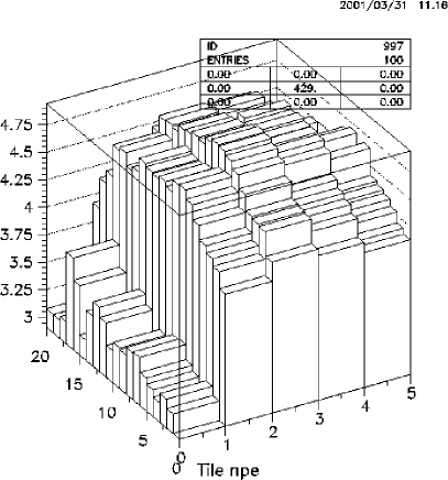
Figure 9.27: Photon yield uniformity over a 1cm-wide strip.

Photo-electron yield of 1mm-thick scintillator for EM calorimeter was measured for 10cm$\times$10cm tiles. It also had a $\sigma$-groove, and 0.7 mm$\phi$ WLS fiber was used. The average photo-electron yield was obtained to be three as shown in Fig.9.26. This corresponds to 350 p.e./GeV for compensating calorimeter, and is not sufficient for EM calorimetry. Comparison between 20cm$\times$20cm$\times$2mm-thick tiles and 10cm$\times$10cm$\times$1mm-thick tiles suggests that photo-electron yield is inversely proportional to the area of tiles, since we know from independent measurement that photo-electron yield is proportional to the tile thickness. Smaller tiles such as 5cm$\times$5cm is considered to have sufficient photo-electron yield. This, together with non-uniformity, should be established by further measurement.

R&Ds on another option of finer-granularity EMC, made of stacks of scintillator strip arrays like SMD, are in progress. This option requires huge number of photo-detector channels, and has become possible by recent advances in multi-channel HPD and EBCCD. Whether we can remove ghosts efficiently or not must be investigated with a full simulator.

Bench tests on strip properties were carried out for various strip sizes with thickness of 2 mm. Non-uniformity of photo-electron yield over a strip was measured to be 4.8% at most for 1cm-wide strips as shown in the Fig.9.27, and is acceptable for EMC. Average photo-electron yield, on the other hand, is 4.6 p.e./MIP. This corresponds to 260 p.e./GeV in the case of compensating EMC, and needs further improvement. However, if software compensation is possible even with the orthogonal $\theta-\varphi$ strip layout, thicker strips can be used, and photo-electron yield will not be a problem. Detailed full simulation studies are again needed to examine applicability of software compensation for this scheme.

9.3.4 Preshower and Shower-max Detectors

The purpose of PSD and SMD are to identify $e/\pi^{\pm}/\gamma/\pi^{0}$, and improve cluster separation and track-cluster association. For this purpose, fine segmentation is necessary for SMD. First we studied SMD of Si-pad array as HES[14] of ZEUS. Test modules were made with Si-pad array firstly with pad size of 1cm$\times$1.5cm and array size of 18$\times$12, then secondly with pad size of 1cm$\times$1cm and array size of 16$\times$16 with improved readout electronics. Beam tests were carried out in combination with PSD and hadron calorimeter modules[15].

Later on, we moved to the scintillator-strip option since:

• Si-pad SMD was thought to cost too much;

• Scintillator-strip SMD used the same technique as the tile/fiber calorimeter, and was easily integrated with calorimeter.

Since the size of the 3Tesla-version baseline JLC calorimeter is now much smaller than the previous one, the first reason may be no more true. However re-examination of the possibility of Si-pad option has not yet started.

   

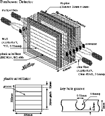
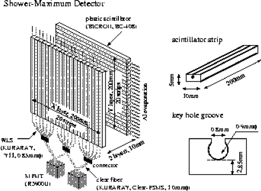
Figure 9.28: Schematical drawing of PSD (left) and SMD (right).

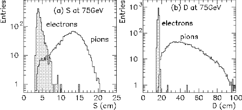
Figure 9.29: e/$\pi$ separation capability of $S$-variable (left) and $D$-variable (right).

According the the baseline design, we built test modules of PSD and SMD, and carried out a beam test at FNAL in combination with the tile/fiber hadron calorimeter[16]. The designs of PSD and SMD modules are schematically shown in Fig.9.28. Photons from scintillators were read out by WLS fiber assembly in both PSD and SMD. In the case of SMD, fibers were connected to multi-channel PMTs, and each strip was read out separately.

In order to separate electrons from pions, three variables are defined:

• $S$ is a measure of lateral shower spread defined as $S=\sqrt{\sum_{i}d_{i}^{2}E_{i}/E_{tot}}$

• $D$ is a measure of longitudinal shower distribution defined as $D=\sum_{j}z_{j}E_{j}/E_{tot}$

• $R$ is a ratio of energy in PSD to total energy.

Examples of $e/\pi$ separation capability of $S$ and $D$ variables are shown in in Fig.9.29. It is seen that $D$-variable has excellent performance in $e/\pi$ separation, and thus that longitudinal segmentation is quite important. Measured $e/\pi$ separation capabilities are shown in Fig.9.30 and summarized in Table 9.5. Obtained score of mostly better than 1/1000 are comparable to other measurements [17], and is satisfactory.

Hit multiplicity of SMD can also be used to identify electrons. By requiring more than 10 hit-strips out of 40 strips, pion rejection factor of about 10 can be achieved with electron efficiency of 98%. However this has strong correlation with R-value, and is not included in the table 9.5.

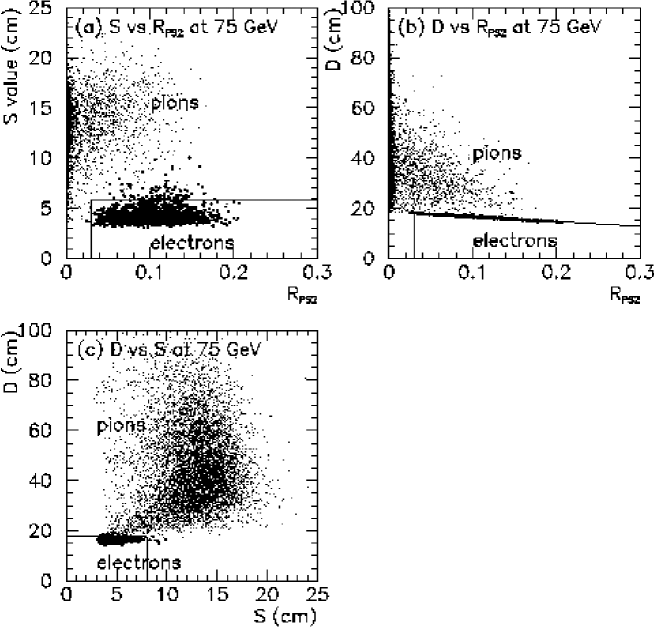
Figure 9.30: e/$\pi$ separation capabilities using combinations of $S$, $D$, and $R$ variables..

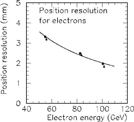
Figure 9.31: Position resolution of SMD.

Table 9.5: Pion rejection factors with the combinations of $R_{PS2}$, $S$ and $D$ values.

Method	$S$ value and $R_{PS2}$			$D$ value and $R_{PS2}$			$D$ and $S$ values
$\epsilon_{e}$ (%)	90	95	98	90	95	98	90	95	98
$r_{\pi}$ at 50 GeV	473	312	180	1274	1104	720	1183	828	753
$r_{\pi}$ at 75 GeV	657	487	343	1258	1162	944	1510	1162	888
$r_{\pi}$ at 100 GeV	984	656	281	1640	1406	1406	984	820	656

Measured position resolution is shown in Fig.9.31. Present result is significantly worse than the baseline requirement of better than 1 mm for energies higher than a few GeV. This is due to saturation and cross talk of multi-channel PMTs, and should be solved before going to the next step.

The WLS fiber assembly costs significant amount of the total cost of scintillator-array SMD. In order to reduce the total cost of SMD, an option which use photo-diodes (PDs) instead of WLS fiber assembly are being studied. Silicon PIN PDs or APDs are attached at the both end of the strips, and photons are directly read out by the PDs. Direct punch-through of charged particles will be identified by double-layer scheme; a blind PD is pasted behind the detector PD.

Studies so far indicates that PIN PDs do not have enough sensitivity, and studies with APDs are in progress. Much more studies are needed to get some conclusion on this option.

9.3.5 Photon Detectors

The whole calorimeter system is designed to be located inside the superconducting solenoid. Thus photon detectors operational in strong magnetic field are needed. In the case of crystal calorimeter, the light yield is large and popular PIN silicon photodiode or APD can be used. On the other hand, in the case of sampling calorimeters, especially compensating calorimeters, the light yield is relatively poor and high-gain high-sensitivity photo-detector is needed.

One conventional solution is fine-mesh photomultiplier tubes (FMPMTs). This has been widely used for magnetic field below 1 Tesla. Possibility to improve its performance at higher magnetic field was first investigated.

Another option is hybrid devices such as Hybrid Photodiodes (HPDs) or Hybrid Avalanche Photodiodes (HAPDs). Performances of such devices have been extensively studied so far. As the result, these hybrid devices are thought to be the best option at present.

1) FMPMT

In order to keep high gain even in the magnetic field of higher than 1 Tesla, high-gain FMPMTs with 24-stages of dynodes (Hamamatsu H2611SXA) were made and tested with magnetic field up to 2.5 Tesla using SKS spectrometer at KEK [18]. Fig.9.32 shows magnetic field dependence of the gain. It still had gain of $3\times 10^{5}$ at 2.5 Tesla when the angle between the PMT axis and magnetic field was 30^∘ even after rapid drop of gain with magnetic field. By extrapolation, it was expected to have gain of $3\times 10^{4}$ at 3 Tesla. However the gain variation with respect to field strength and PMT angle to the field direction is quite steep. This feature is not desirable, though is not fatal. We therefore concluded that FMPMT can not be the primary solution.

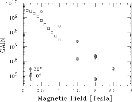
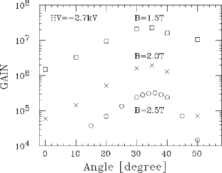
Figure 9.32: Magnetic field dependence of FMPMT gain. Horizontal axes are magnetic field strength (left) and angle between magnetic field and PMT axis (right).

2) Hybrid Devices

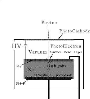
Figure 9.33: Schematic view of the HPD structure.

HPD consists of a photo-cathode and a PIN photodiode facing to each other with a narrow vacuum gap in between. This is essentially insensitive to the axial magnetic field as is easily seen from the structure shown in Fig.9.33. High-voltage is applied between the photocathode and the PIN silicon diode. Emitted photoelectrons are accelerated by this field, and injected to the PIN diode. Those photoelectrons deposits their energy when they pass the depletion layer and create electron-positron pairs. Roughly speaking, since excitation energy of one electron-position pair is 3.6 eV, gain of 3000 is expected with photo-cathode voltage of -11 kV. Actual gain is slightly lower due to the surface layer of the diode.

HAPD uses APD instead of PIN photodiode, and has higher gain due to the gain of APD itself. With an APD of gain 100, HAPD would achieve total gain comparable to PMTs.

             

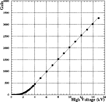
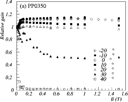
Figure 9.34: Gains of high-gain HPD out of (left) and in (right) a magnetic field.

     

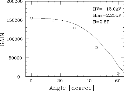
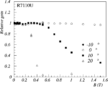
Figure 9.35: HAPD gain in a magnetic field for API 748-73-75-631 (left) and for Hamamatsu R7110U. Solid line in the left figure is result of calculation.

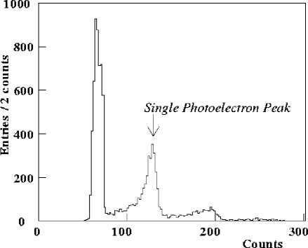
Figure 9.36: Single photo-electron peak measured outside of magnetic field by Hamamatsu R7110U.

Properties of HPDs and HAPDs have been extensively studied so far [18, 19]. Gains of an HPD (Delft PP350F) in and out of magnetic field are shown in Fig.9.34. The gain in the magnetic field with $V_{PC}$=-15 kV was measured to be 4000. If we assume the photo-electron yield of EMC to be 260 p.e./GeV, preamp noise to be 1000 $e^{-}$, and HPD gain of 4000, we can achieve readout noise of about 1MeV.

Though the gain of HPDs is high enough for calorimetry, it is not high enough for PSD and SMD. We therefore studied performances of HAPDs. The gains of HAPDs were measured for 748-73-75-631 made by Advanced Photonix and for Hamamatsu R7110U in magnetic field. The results are shown in Fig.9.35. It is clearly seen that HAPDs are operational in a magnetic field with high gain. It was also established that HAPDs had sensitivity to measure single photon as shown in Fig.9.36. Therefore HAPDs can be a good candidate for PSD readout.

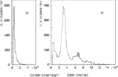
Figure 9.37: Single-photo-electron peak measured with electro-focus EBCCD by RD46.

Scintillator-strip SMD requires ultra-multi-channel photon detectors. Though once Advanced Photonix made 9-pixel HAPDs, it is not so easy to make multi-pixel HAPDs. Multi-channel HPDs are available with order of 100 channel/device at present. However sensitivity of HPDs are not high enough to use for SMD. Recently developed EBCCDs are ultra-multi-pixel devices naturally, and can achieve single-photon sensitivity [20, 21]. This is thought to be the best candidate for SMD, and basic surveys have been initiated. RD46 collaboration has succeeded to observe single photo-electron peak with an EBCCD as shown in Fig.9.37. However it is an electro-focus type like image intensifiers, and can not be used in a magnetic field. We therefore started performance study on proximity-focused EBCCDs[20]. Structure of proximity-focused EBCCD is quite similar to that of HPDs shown in Fig.9.33, replacing PIN silicon photodiode by a CCD. Photo-electrons bombard back-side of CCD, where substrait is thinned to enable photo-electrons to reach to the epitaxial layer. Fiber bundle with appropriate fiber spacing is attached to the photocathode window, and hits are reconstructed by clustering algorithm. Fig.9.38 shows gain curve with respect to the applied photo-cathode voltage and noise vs. temperature. Measured sensitivity is yet unable to detect single photon, and further studies are in progress.

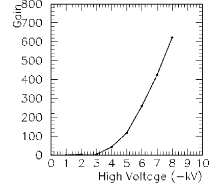
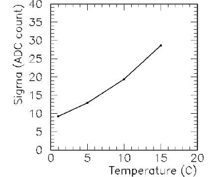
Figure 9.38: Gain vs. photo-cathode voltage (left) and noise vs. temperature (right) for proximity-focused EBCCD N7220.

9.3.6 Engineering R&Ds

There are several engineering issues related to the actual construction of the calorimeter system:

• Rigid and strong lead alloy;

• Mass production scheme and cost of tiles;

• Mass production scheme and cost of WLS assembly;

• Overall structure.

Most of these are yet open questions.

Lead Alloy

Our baseline design is to use lead alloy as absorber material because of its high-$Z$, density and cost. However lead is very soft metal, and development of rigid and hard lead alloy is indispensable.

Figure 9.39: A photo of the setup to measure mechanical properties of lead alloys. Broken test piece after measurement is seen.

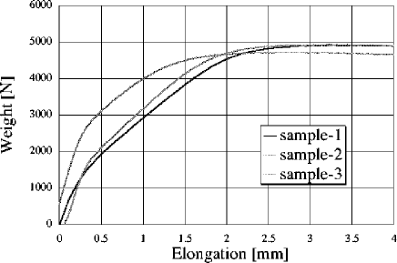
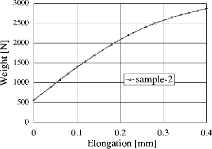
Figure 9.40: Elongation vs. applied weight for a Ca-doped lead alloy. Left figure shows whole curve which gives yield tensile strength, and right figure shows rising region which gives Young modulus.

Lead with Sb or with Ca/Sn are the most popular hard lead alloys. It is also well known that heat treatment and/or mechanical treatment improves mechanical feature for some lead alloys. In order to study these properties, test pieces made of Pb(Ca/Sn) and Pb(Sb) alloys of several different concentrations have been made, and measurement of strength, Young’s modulus, and creep are in progress. Properties of heat treatment and mechanical treatment are also under study.

Fig.9.39 and Fig.9.40 show the measurement system and a result of strength measurement for a Ca-doped lead alloy, respectively. Tensile strength (yield) of this sample is measured to be 49MPa, which is 7 times stronger than pure lead. However measured Young modulus of 13GPa is almost the same as that of pure lead.

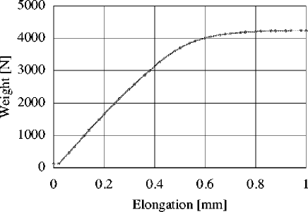
Figure 9.41: Elongation vs. applied weight for mechanicaly-treated lead alloy. Elastic region extends to higher tension region, while slope itself (Young modulus) stays the same.

Improvement of tensile strength itself is not an important result because one can not use material beyond elastic region. Fig.9.41 shows how mechanical treatment improves elastic region of lead alloy.

Studies on heat treatment is in progress.

Feasibilities of other options such as tungsten, copper, stainless steel or hybrid material such as CFRP-sandwiched lead are yet open questions.

Mass-Production of Tiles and WLS Assemblies

Machining of $\sigma$-grooves on tiles costs about $10/tile for fabrication scale of a few thousand pieces. Since there are 2.2 million tiles in total, machining cost is significantly high and should be decreased. This can be solved by making tiles with casting. However, casting of tiles with $\sigma$-grooves seems very complicated, though is not thought to be impossible. On the other hand, the strip-EMC option enables quite easy casting. Drastic cost reduction is expected by mega-strip casting ; casting of the strip array as a whole. This possibility should seriously be pursued.

Cost reduction of WLS assembly is yet an open question. Direct readout by attached photo-diode, which is under study as a part of the shower-max detector R&D, may enable us to avoid this problem.

Structural Study

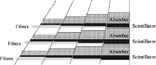
Figure 9.42: Conceptual layout of constant-sampling barrel calorimeter.

There are two major ways to build the barrel calorimeter assembly. One is a stack of doughnuts, and the other is an assembly of orange sectors. Orange sector assembly is a natural solution for z-insertion of mega-tiles. In this case, however, absorber plate orientation can not be perpendicular to the polar angle direction. Therefore sampling frequency, and accordingly energy resolution, becomes $\theta$-dependent. One way to avoid this problem is to make a structure as shown in Fig.9.42. This layout enables constant sampling frequency and at the same time reserving room for clear fibers, which increases as $\theta$ increases. However mechanical strength should be a very difficult problem. Simulation study is needed to estimate the effect of $\theta$-dependent resolution on physics capabilities.

9.4 Simulation Study

A full simulator (named JIM) based on GEANT3 was constructed for detector parameter optimization and performance study. Calorimeter geometry and parameters listed in the Table 9.2 are implemented, together with all other detectors and structural components. Calorimeter signal normalization, response mapping, linearity and energy resolution examinations have been done by comparing with the beam test results. Development of hadron-shower clustering algorithm is in progress

Simulator Tuning

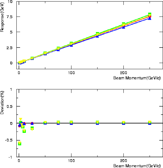
Figure 9.43: Linearity of the calorimeter implemented in a full simulator. Red, green, blue, and yellow lines indicates barrel CAL response to electrons, barrel CAL response to pions, endcap CAL response to electrons, and endcap CAL response to pions, respectively.

Linearity of calorimeter response is shown in Fig.9.43. It has an excellent linearity of less than 0.3% from 2GeV up to 250GeV, while 1GeV data has slightly large deviation probably due to cross section of hadronic reaction and low multiplicity of shower at low energy.

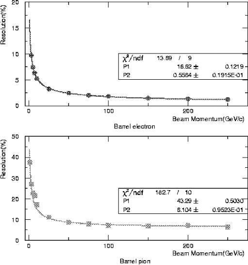
Figure 9.44: Energy resolution of barrel calorimeter implemented in a full simulator. Top is for electrons, and bottom is for pions

Fig.9.44 shows full simulation result of the energy resolution of barrel calorimeter for electrons and for pions. Obtained hadron energy resolution of $43.3\%/\sqrt{E}\oplus 6.1\%$ for pions has much worse constant term than our beam test results shown in Fig.9.22. It has already been shown that this is not due to shower leakage in the simulation. More tuning of detailed geometry and/or cross section of physics processes are necessary to reproduce measured results.

 

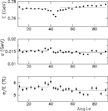
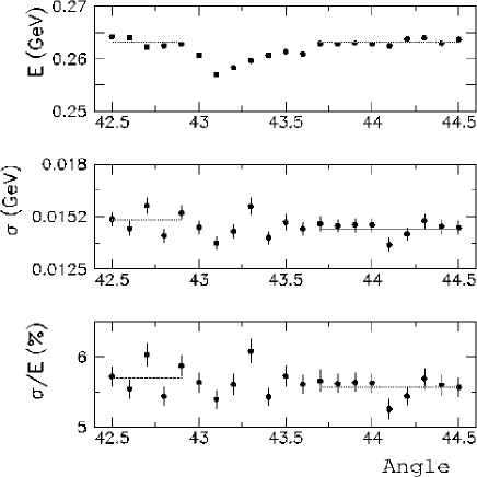
Figure 9.45: Calorimeter response vs polar angle obtained by 10 GeV electron injection. Dips in the left and right figures show boundary between the endcap and barrel calorimeters and boundary between barrel super-towers, respectively.

Response mapping was also done using electrons with respect to the polar angle as shown in Fig.9.45, and to the azimuthal angle. We observe a dip in energy measurement at the super-tower boundary. The beam test data, on the other hand, shows enhancement rather than dip as shown in Fig.9.25. This difference is considered to be caused by two reasons: 1)non-uniformity of photo-electron yield over a tile is not implemented into the full simulator, and 2)there exists unexpected gap between supertowers in the geometry definition. The latter was found by difference of response map between electron injection and positron injection, and should be fixed. Impact of non-uniformity on physics analysis should be investigated to know necessity to implement non-uniformity into the full simulator.

Hadron Shower Clustering

 

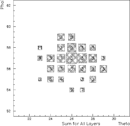
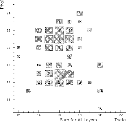
Figure 9.46: Hit-cell distribution for one-pion injection (left) and for two-pion injection (right), and results of 3-D contiguous clustering. One box corresponds to one calorimeter cell, but longitudinal layers are projected to 2-D. The size of the boxes correspond to the energy in log-scale. Overlapped numbers indicate serial cluster number.

Clustering of hadron shower is essentially important for precise track-cluster association. Conventional clustering (JADE algorithm) for EM shower does not work very well for hadron showers because it tends to split one shower into plural clusters, and thus leaves excessive neutral energy undeleted.

There are two possibilities to avoid this problem; one is to make large contiguous cluster with plural peaks in it, and the other is to make ’super-cluster’, a cluster of single-peak clusters. The former method with two-dimensional clustering is very successful for quick-simulation results, but does not work well for full-simulation data. Extension of this method to 3-dimensional clustering is first tried. The latter, which has been studied by TESLA group, has not yet been tried.

Fig.9.46 shows how this clustering works on a hadron shower induced by one 100GeV-pion (left), and two 100GeV-pions (right). Boxes indicate a tower, and the sizes represent the energy. Numbers overlapped on boxes are cluster ID numbers. Some contiguous towers have different cluster ID, which means that individual cells in the towers are not contiguous in 3-D space.

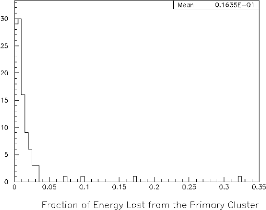
Figure 9.47: The fraction of the energy summed over satellite clusters to the total measured energy.

Several satellite clusters are made around/apart from the main cluster. These satellite cluster are not deleted at the track-cluster association stage, and thus result in excessive neutral energy. The fraction of the energy summed over satellite clusters to the total energy are shown in Fig.9.47 for one-pion events. There are four events with large satellite energy. However total satellite energy is only 1.6% of the total energy even with the four events, and most of the energy are collected by the main cluster.

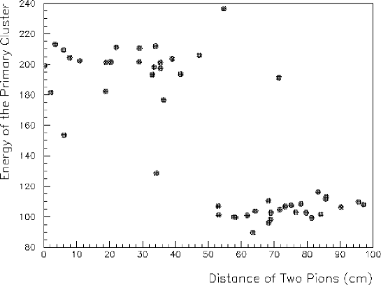
Figure 9.48: Energy of the primary cluster as a function of distance between two pions of 100GeV. 200GeV means two pions formed one connected cluster.

Right figure of Fig.9.46 shows merit of contiguity check in 3-D space. Two clusters looks contiguous in 2-D projection, but are not in 3-D space, and thus correct clustering is performed. Figure 9.48 shows separation capability of two pion clusters made by 100GeV pions. Two clusters can be reconstructed separately down to about 50cm-distance, which corresponds to four hadron cells. It means at least one vacant cell is needed between two $3\times 3$ clusters. Thus present score is almost at the geometrical limit.

Two pions with less distance mostly result in one cluster in this 3-D contiguous clustering. In this case, existence of two pions must be identified by shower-max detectors, and energy decomposition may be done by momentum-energy subtraction. This, however, gives worse energy resolution than geometrical cluster decomposition. To avoid this deterioration, conventional JADE algorithm can be tried only for such cases. This method is yet under development.

Study of effect on physics sensitivity be forthcoming.

9.5 Future Prospect

Results of quick simulation for various physics processes have demonstrated that the baseline calorimeter system can realize excellent physics sensitivity. However, validation with a full simulation is essentially important, especially for optimization of granularity. This must be completed urgently.

Extensive hardware studies have proven the technical feasibility and performance of tile/fiber scheme with hardware compensation. There are still open questions in high-granularity EMC option and in photon detector options. These issues are also related to the total cost, and thus should be solved before moving to the proto-type R&D stage. Engineering studies including the heavy metal choice should also be finished before the proto-type stage.

Chapter 10 Muon detector

10.1 Introduction

The muon momentum can be precisely measured by the inner tracking detectors. Therefore the muon detector should only have many position measurements to obtain good matching with the tracks, where modest position resolution is required. Modest timing resolution is also required to reject cosmic ray backgrounds. As the requirements are much looser than those for the LHC experiments, we think that we can construct the muon detector with existing detector technologies. We may apply new technologies developed for LHC if required.

Fig. 10.1 is a cross sectional view of the standard detector, where the muon detector layout is shown. In the barrel region the solenoid magnet is surrounded by one layer of plastic scintillator counters, followed by six muon detector layers; one layer just inside the return yoke, four layers in the return yoke, and one layer just outside the return yoke. The endcap muon detectors have a similar detector configuration. The total area of the muon layers amounts to about 4,000 m².

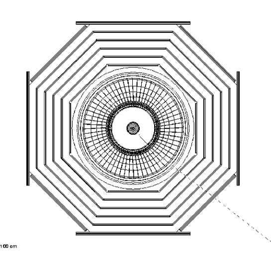
Figure 10.1: Layout of the muon detector.

10.2 Material Effect

We studied the effect of the detector material to the muon detector. Table 10.1 summarizes the amount of material of the standard JLC detector in front of the return yoke and in the return yoke itself at $\theta=90^{\circ}$. The muon momentum is required to be more than 2.2 GeV to reach the return yoke, and to be more than 5.2 GeV to fully penetrate the return yoke.

Table 10.1: Material thickness of the detector at $\theta=90^{\circ}$. Those in front of the return yoke, in the return yoke itself, and the total thickness are listed.

	In front	Return Yoke	Total
Weight	1.09 kg/cm2	1.51 kg/cm2	2.60 kg/cm2
Radiation length	158 $X_{0}$	109 $X_{0}$	267 $X_{0}$
Interaction length	5.6 $\lambda_{0}$	11.2 $\lambda_{0}$	16.8 $\lambda_{0}$

Multiple scattering due to the material in front of the muon detector is simulated by JIM [2], the full simulation program of the JLC detector. In the simulation, muons are generated at the interaction point with a momentum of $(p_{x},0,0)$ where the $+z$ direction is along the electron beam. The hit positions at the inner surface of the return yoke ($x=500$ cm) are recorded.

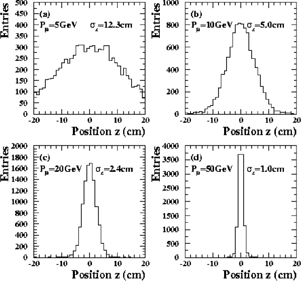
Figure 10.2: Distributions of the $z$-coordinate at the return yoke surface (a) $p_{\mu}=5$ GeV, (b) $p_{\mu}=10$ GeV, (c) $p_{\mu}=20$ GeV, and (d) $p_{\mu}=50$ GeV.

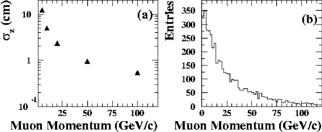
Figure 10.3: (a) The standard deviation of the $z$-coordinate at the return yoke surface as a function of the muon momentum, and (b) the distribution of the muon momentum in the $b$-quark pair production at ${s}=500$ GeV.

Fig. 10.2 shows the distributions of the $z$-coordinate for muons with initial momentum of 5, 10, 20, and 50 GeV. The distributions of the $y$-coordinate are very similar to those of the $z$-coordinate. Fig. 10.3(a) shows the standard deviation of the $z$-coordinate ($\sigma_{z}$) due to multiple scattering as a function of the muon momentum. This result is similar to that obtained for the TESLA detector [3]. Fig. 10.3(b) shows the momentum distribution of muons in the $b$-quark pair production at $\sqrt{s}=500$ GeV. As seen in this histogram the majority of muons have momentum below 50 GeV, for which $\sigma_{z}$ is larger than 1 cm. We thus conclude that the position resolution of about 1 cm is sufficient for the muon tracking device.

10.3 Detector Options

The JLC muon detector should have position resolution of 1 cm or better, and should be constructed with a well-established technology. In addition, as the muon detector covers a very large area, the technology must be inexpensive. Single-cell drift chambers, resistive plate chambers, and thin gap chambers are currently considered as the candidates.

10.3.1 Single Cell Drift Chambers

The first candidate, single-cell drift chambers (SCDCs), is described in the JLC-I report [1]. A SCDC super-layer has four layers with xx’yy’ wire configuration to measure both $\phi$ and $z$ coordinates. The cell size of the SCDC is $10\times 5$ cm², and the wire length is $10\sim 15$ m. A wire support is located at the middle of the wire to reduce the wire sag. The expected position resolution is about 500 $\mu$m dominated by the gravitational wire sag. Once the hit coordinate along the wire is known, the position resolution can be much improved. The number of readout channels is relatively small, about 10,000 in total.

10.3.2 Resistive Plate Chambers

The second candidate is resistive plate chambers (RPCs). Large area RPC systems are used by experiments at B-Factories [4, 5], and will also be used by experiments at LHC [6, 7]. Such a large area RPC system can be constructed with a very low cost, because of their simple structure with no wires. The RPC can be very thin, for example, the total thickness of an RPC doublet for the BELLE KLM detector is only 3.2 cm. The position resolution is determined by the dimensions of readout cathode strips, and a resolution of 1 cm can easily be achieved. RPC is a very promising candidate for the JLC muon detector.

10.3.3 Thin Gap Chambers

The third candidate is thin gap chambers (TGCs), a kind of MWPC with a very thin gap ($\sim 3$ mm). TGC is highly efficient except for the dead space due to wire supports. The signal is fast enough for our purpose. The position resolution of 1 cm is easily achieved, similar to the case of RPC. TGC can be operational at a very high particle rate of 1 kHz/cm². The only demerit is the higher construction cost than that of RPC, as TGC uses a huge number of wires.

The endcap muon trigger system for the ATLAS experiment uses the TGC technology [6]. To this purpose intensive R&D works were performed in Israel and Japan. Production of a total of 1,000 large TGC doublets/triplets are in progress at KEK. According to the ATLAS TGC schedule, the production will be completed in 2003, and then installed at the LHC experimental hall by the end of 2004. Through the TGC production we will at least gain an excellent experience to construct a large area muon detector system.

10.4 Summary

A simulation study is made to investigate the effect of the detector material to the muon detector. The position resolution required for the muon tracking device is found to be about 1 cm.

The detector technology is still to be determined, We have currently three possible candidates for the muon tracking device; single-cell drift chambers, resistive plate chambers, and thin gap chambers. The technology will be determined by further simulation studies, together with experiences obtained at B-factories and LHC.

Chapter 11 Detector Magnet

11.1 Superconducting coil

A superconducting solenoid magnet has been studied for the JLC detector. The JLC superconducting solenoid magnet is shown in Fig. 11.1. The magnet provides a central magnetic field of 3T at nominal current of 4725A in a cylindrical volume of 8m in diameter and 6.8m in length. It placed outside the calorimeter to achieve good hermetic. The coil consists of double layer aluminum-stabilized superconductor wound around the inner surface of an aluminum support cylinder made of JIS-A5083. At the both of the end part, four layers of coil will be wounded to improve field uniformity in the CDC volume. Length of the end part is 1.1m. Indirect cooling will be provided by liquid helium circulating through a single tube welded on the outer surface of the support cylinder. Since the magnet is located outside of the calorimeter, it is not necessary to design as a thin superconducting solenoid magnet. Therefore, a thickness of outer/inner wall of cryostat can be thick as much as sub-detectors are necessary.

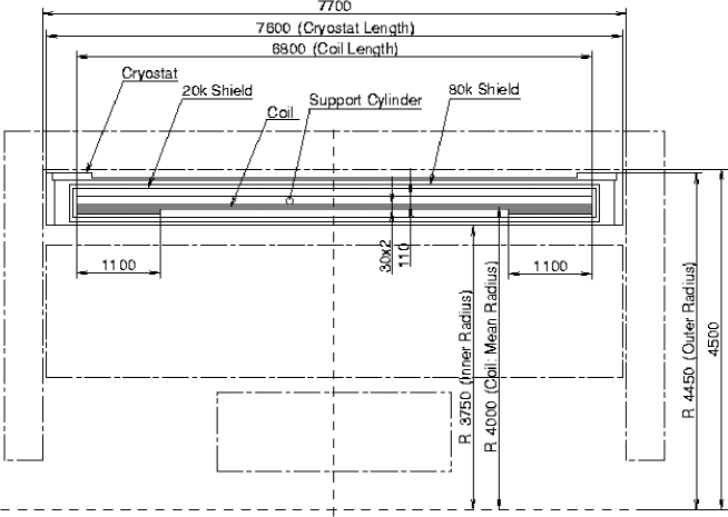
Figure 11.1: Configuration of the JLC superconducting solenoid magnet.

It was considered about a superconducting wire for the JLC solenoid based on the ATLAS superconducting wire. The size is 4.3mm width and 30mm height. On design of a superconducting solenoid, it is required to be reliable two main mechanical stresses, hoop stress and axial stress in a coil. The evaluation is done by calculated combined stress. Even though the yield strength of superconducting wire is achieved to around 250MPa at recent R&D of high strength superconducting wire, it assumed to yield strength of 150MPa in our design. The combined stress, Von Mises, in the coil when the central magnetic field of 3T is shown in Fig. 11.2. Since the calculation result, required thicknesses to keep within yield strength in the coil are to be 110mm for support cylinder and 60mm for coil, respectively. From these required thickness, the cold mass is approximately to be 95tons. The stored energy is calculated to be 985MJ.

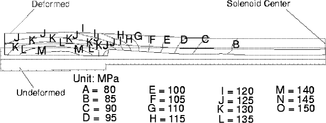
Figure 11.2: Stress and deformation shape due to magnetic force in the coil.

To protect the coil due to the magnet quench is one of the most important issues for solenoid design. Figure 11.3 shows the temperature rise and current decay after magnet quench in case of mounting pure aluminum strips. In this calculation, total magnetic energy is dumped entirely into the superconducting wire, and it assumed that the pure aluminum strips are mounted on the inner/outer surface of the solenoid. By mounting pure aluminum strips, the quench propagation velocity can be increased drastically. As the calculation results, the maximum temperature rise after quench is to be around 80K, and the magnet current is decayed within 80 second from the nominal current of 4725A.

Figure 11.3: Quench behavior of the coil with pure aluminum strips.

Radiation shields consist of 20K-shield and 80K-shield are placed between the coil and the vacuum vessel. These shields have to be decoupled electrically from both the coil and the vessel walls in order to avoid the effects of the eddy current induced by the fast current discharge of the coil. The vacuum vessel for this solenoid magnet consists of inner and outer coaxial cylinders that are connected by flat annular bulkheads at each end. The solenoid magnet will be supported at the innermost layers of barrel iron yoke by fixing the support structure on the outer vacuum vessel. The coil support system has to be transmitting both the weight of cold mass and the magnetic de-centering forces. If the geometrical center of the solenoid and the iron yoke are deviated each other, the magnetic force is generated. This force has to be taken into account on the coil support design.

11.2 Iron structure

11.2.1 Introduction

An iron structure for the JLC detector has been studied and designed. Figure 11.4 shows the basic configuration of the JLC iron yoke structure. The structure consists of the barrel and two end-yoke sections. The overall height is about 16m from the floor level; the depth is about 13m. The iron structure will be made from low-carbon steel (JIS-S10C: 0.008 0.012 wt% carbon). The total weight except for sub-detectors is approximately 11,000tons, and it will be placed on a transportation system for roll-in/out. Assembling of the iron yoke and installation of the sub-detector will be carried out at the roll-out position and then move to the roll-in position for the experiment. The end-yoke separates at its center and then opens to access to the sub-detectors.

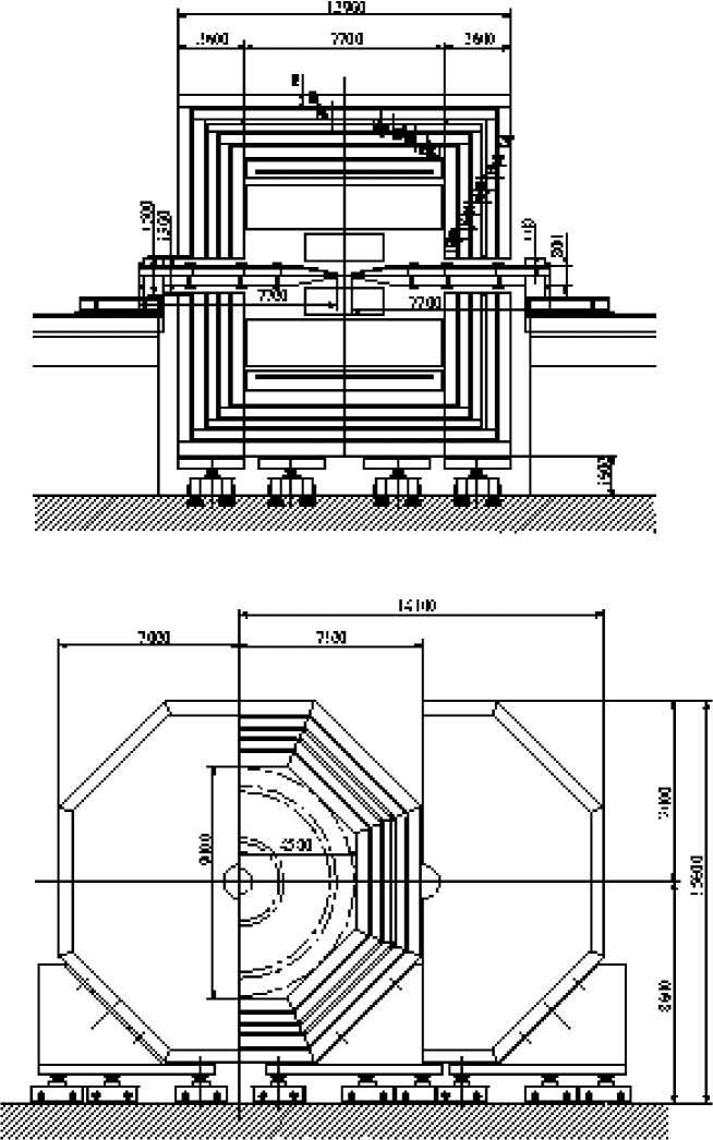
Figure 11.4: Basic configuration of the JLC iron yoke.

Some kinds of design studies are required to optimize the iron yoke configuration. Those are the influence of the magnetic field, stability against the acted forces such as self-weight of iron yoke (mechanical design) and assembling/maintenance consideration. In the magnetic field study, the iron yoke is acted on the magnetic field of 3T from the JLC solenoid magnet, amount of iron have to be determined for improving the field uniformity in the CDC volume, and leakage field outside of the iron yoke is kept minimize by absorbing the flux return. In the mechanical design, it is required to study on the deformation and stress level against heavy self-weight of iron yoke and strong magnetic force. As the other important issue for the mechanical design, an earthquake resistant design is required. In these studies, way of iron yoke assembling, access to the sub-detectors and cables pass have to be taken into account.

11.2.2 Magnetic Field Design

The criteria for the magnetic design to determine the iron yoke structure are around field uniformity of 1% in the CDC volume, and an allowable leakage field at 10m far from the solenoid center is less than 100 gauss. To set the tolerance against leakage field, an important criterion is to work an electromagnetic valve. With keeping these requirements, thickness of the iron plates were tried to minimize as possible. Permeability of iron plate for calculation is shown in Fig. 11.6. This is the measurement data of the BELLE iron yoke, which is the same material as the planning JLC iron yoke. The ways to improve the field uniformity without increasing the amount of iron are coil thickness at the end of the solenoid is thicker, and the inner diameter of the end-yoke is smaller. The results of magnetic field calculation when the central magnetic field of 3T is shown in Fig. 11.6. In this calculation, the end part of the coil is two times thicker than the other part. The maximum magnetic field in the iron yoke is to be 3.3T. The field uniformity is to be 1.2% as show in Fig. 11.8. The magnetic field along the beam line is shown in Fig. 11.8. The leakage field was calculated to be 110 gauss.

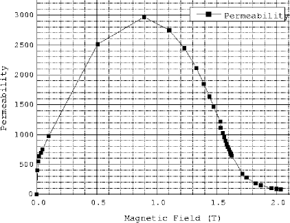
Figure 11.5: Permeability of iron material (JIS-S10C), which was used for the magnetic field calculation.

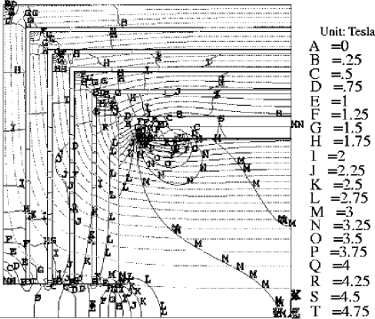
Figure 11.6: Calculated magnetic field at the central magnetic field of B=3 T.

From this calculation, iron plate thicknesses of barrel and end-yoke were optimized. Innermost and outermost layers of yokes are understood to require a thicker iron plate of 50cm-thick than other layers plates of 30cm-thick and 40cm-thick.

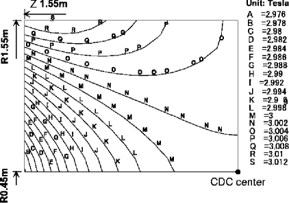
Figure 11.7: Field uniformity in the CDC volume at B=3T. The uniformity is simply calculated from the ratio of the minimum and maximum fields.

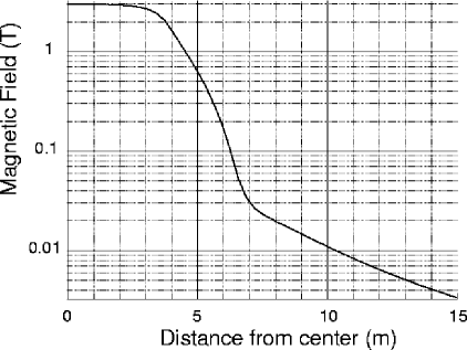
Figure 11.8: The magnetic field along the beam axis at B=3 T.

11.2.3 Mechanical Design

Load conditions of iron yoke are self-weight of 11,000tons. The barrel-yoke is about 5,000 tons and the end-yoke is 6,000 tons, respectively. The magnetic force was calculated to be 18,000 tons. The mechanical design will be followed to the design guideline for construction of nuclear power plant in Japan. In this reference, the safety margins for various stresses are indicated and load conditions are also indicated at the various situations. At the earthquake resistant design, an input acceleration will be 0.2G or 0.3G. Earthquakes of this magnitude are expected to occur in the Tsukuba area with a frequency of once per year of 30 years. Figure 11.10 shows the deformation of the outermost layer of the barrel-yoke due to self-weight. The self-weight of the outermost layer is approximately 1,352 tons. The maximum deformation was calculated to be 3.1mm. However, it should be noticed that this assumption is ideal conditions. The practical situation is each octagonal section will be assembled by bolted joints, so its stiffness must be lower than the complete octagonal shape. It is important to assemble with keeping the rigid structure. The gravitational sag of end-yoke due to the self-weight will be neglected. Because the self-weight is acted on the vertical direction, the end yoke is the rigid body in this direction.

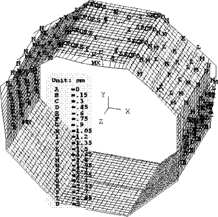
Figure 11.9: Deformation of the outermost layer of the barrel-yoke due to self-weight of 1,352 tons.

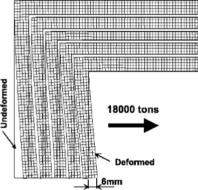
Figure 11.10: Deformation of the end-yoke due to magnetic force of 18,000 tons.

The deformation of the end-yoke due to the magnetic force of 18,000 tons is shown in Fig. 11.10. The maximum deformation was calculated to be 6mm. The end yoke will be assembled from 4 sections from the viewpoint of crane capacity and easy assembling, it will not be able to expect to the stiffness as the completed octagon. At the earthquake resistant design, the natural frequency of iron yoke is calculated as the first step. If this value is lower than the 10Hz, the reinforcement of the iron yoke structure is required due to avoid to resonant with earthquake. As the next step, various earthquake waves those maximum magnitudes are corresponding to 0.2G or 0.3G are input to the iron yoke, then get the responded magnitude. If the magnitude is 0.4G, this value is applied to the horizontal direction as the static load. At the final step, the deformation and stress level will be calculated using 0.4G.

11.2.4 Configurations

The barrel-yoke structure is constructed from eight flux-return and eight Muon detector modules. Each barrel Muon module consists of 5 layers with 100mm thick instrumental gaps. Thicknesses of steel plates are 500mm, 400mm, 300mm, 400mm and 500mm from innermost layer, respectively. Few millimeters of flatness of steel plate has to be taken into account on the Muon detector design. To improve the stiffness of the barrel-yoke, some support structures will be necessary.

Each end-yoke is planned to separate into four quadrants containing five iron plates. Each thickness is the same as the corresponding plate of the barrel-yoke. The inner diameter of 1,300mm is required for th e support tube. The end-yoke must slide out to provide access to the inner detector. An end-yoke transport system has to be studied.

Chapter 12 Monte Carlo Simulation Tools

12.1 Overview

Monte Carlo simulation comprises an essential part of any modern experimental high energy physics. In the designing stage of a large scale project such as the JLC, its primary goal is to identify important physics targets and then set machine parameters such as beam energy, luminosity, beam energy spread, beamstrahlung, beam related background, etc. and detector parameters such as momentum resolution for charged particle tracking, calorimetric energy resolution, impact parameter resolution, minimum veto angle, particle identification, and so on. These performance requirements constrain the machine and the detector designs eventually to be integrated into a TDR. The simulation studies thus link three major components of the project: physics, machine, and detector. It is therefore very important to simulate, with sufficient accuracy and speed, all of key features of linear collider experiments.

Monte Carlo simulation that connects physics, machine, and detector parameters has the structure shown in Fig.12.1.

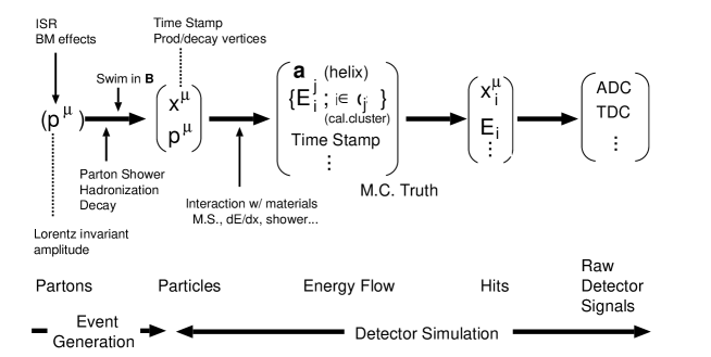
Figure 12.1: Flow chart for Monte Carlo simulations

We start from 4-momenta of initial partons generated with initial state radiation (ISR) and beam effects. After parton showering, hadronization, and decays we are left with pairs of two 4-vectors $(x^{\mu},p^{\mu})$ for final state particles, where $x^{\mu}$’s carry information on production and decay vertices as well as time stamps. These particles are swum in the detector volume, interacting with materials, leave tracks in tracking devices and, depending on the nature of the particles, shower in calorimeters. These tracks are usually parametrized as helices and individual showers as calorimeter clusters, resulting in hits in the tracking devices and energy deposits in calorimeter cells. If necessary we can then convert these into raw detector signals such as ADC or TDC values, etc.

There is a mirror image of this flow diagram, which is called event reconstruction and analysis, and is shown in Fig.12.2.

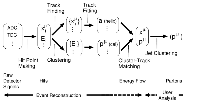
Figure 12.2: Flow chart for event reconstruction and analysis.

From the raw data signals we make hit points (hit point making). In the case of hits in trackers, the map from the set of individual hits to subsets of hits (tracks) is called track finding, while in the case of calorimeter hits, the map is called clustering. The map from the tracks to helix parameters is called track fitting. These tracks and calorimeter clusters are combined through track-cluster matching and yield energy flow information. Together with vertex information, these comprise a set of pairs of 4-vectors $(x^{\mu},p^{\mu})$ of the final state particles. Jet clustering follows this step and hopefully leads us to reconstructed initial parton 4-momenta.

Depending on how we short cut these processes from the 4-momenta given by the event generator to the reconstructed 4-momenta, there can be many levels of simulation. It is very useful to do it in various levels, since by doing so we will know the effects of what we skipped or included, thereby leading us to deeper understanding of the detector as well as to fast but sufficiently accurate way of simulation.

In order to facilitate such multi-level simulations, it is desirable to have a general simulation study framework which allows easy switching from one level to another without affecting end users in the analysis stage. Considering the recent advance of object-oriented programming (OOP) paradigm, we are developing a framework called the JLC Study Framework (JSF) which is sketched in the next section. Section 12.3 then lists up various Monte Carlo event generators that can be input to the JSF. Brief description of detector simulators we have used throughout this report is given in Section 12.4. Section 12.5 then discusses future direction.

12.2 JSF: JLC Study Framework

12.2.1 Philosophy

The JLC Study Framework (JSF) is written in C++ and is based on ROOT[1]. As its name suggests, the JSF sets a general framework for event-based data processing, scope of which covers all the JLC-related software works that extend from various Monte Carlo simulations to online data taking and monitoring for beam tests and their off-line analyses. Basic concept of the JSF is to organize an event-based data processing program as consisting of modules. Each module comprises a program unit for a certain task and is implemented as derived from a base class called JSFModule, which specifies a common interface for processing begin run, event, end run data, etc. Any module that inherits JSFModule is automatically included in the sequence of the program execution, which is controlled by a kernel routine, an instance of a class called JSFSteer. The kernel routine also takes care of inputs from and/or outputs to files, and provides a graphical user interface as well as an event display facility.

For Monte Carlo simulation studies, the JSF provides a common interface to various event generators both fast and full detector simulators, event reconstruction, and analysis.

Several modules are thus included in the standard JSF distribution: a base class for event generators using BASES/SPRING[3], an interface to PYTHIA[5], a module to handle parton showering and hadronization using JETSET, and modules to control a quick simulator (QuickSim) and a full simulator (JIM). There are also interface modules to read external event data files such as ASCII text files of parton four momenta, data created by JIM, etc. Their relations are shown in Fig. 12.3.

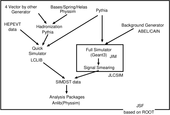
Figure 12.3: Software packages and their relations for JLC studies.

12.2.2 Interfaces to Event Generators

There are interfaces to several types of event generators implemented in the JSF.

Pythia

The Pythia generator module uses the ROOT’s interface to Pythia[5] and is built in the JSF as the standard event generator. Event generation with this module can thus be controlled by a macro file in a standard format or a built-in GUI or both, which specify event types, decay modes, the number of events to generate, etc.

Bases/Spring-based Generators

The Bases/Spring module provides an interface mainly for those generators that utilize HELAS[2] for helicity amplitude calculations. The current version of the JSF comes with a C++ version of BASES/SPRING, where BASES performs integration of amplitudes squared for the process in question and SPRING carries out generation of weight-one events according to the integration result. Resultant partons are passed to a hadronizer described below. Many event generators have been developed using this interface, of which a package called Physsim is described in the next section.

Other Generators

For other event generators which are not integrated into the JSF, two types of interface modules are prepared. One is to read generator data in HEPEVT format. In this case, the 4-momenta of stable particles are directly fed into detector simulators. The other is to read 4-momenta of quarks and leptons, which are prepared in an ASCII text file. This category includes various generators based on GRACE[4]. As with the Bases/Spring-based generators, the generated partons are hadronized using the standard hadronization module, being ready for consumption by a detector simulator. This provides a very handy interface to a toy Monte Carlo.

Beamstrahlung

Proper account of beamstrahlung is indispensable for realistic simulations of experiments at the JLC. The JSF thus provides a standard package that generates average electron and positron energy during collision under the influence of beamstrahlung.

The beamstrahlung spectrum, $F(Z)$, used there is given by

$$F(z)=\int^{1}_{0}e^{-n_{\gamma}\tau}\frac{e^{-\eta}H(n_{1}\eta^{1/3}\tau)}{1-z}d\tau$$ (12.1)

where $z=E/E_{0}$ is the fractional energy of the electron and

$$\xi=\frac{r_{e}^{2}E_{0}N}{\frac{1}{2}m_{e}\alpha\sigma_{z}(\sigma_{x}+\sigma_{y})},\;\;n_{cl}=\frac{\alpha r_{e}N}{\frac{1}{2}(\sigma_{x}+\sigma_{y})},\;\;n_{\gamma}=n_{cl}\left(\frac{1-0.598\xi+1.061\xi^{5/3}}{1+0.922\xi^{2}}\right),$$ (12.2)

$$\eta=\frac{1-z}{\xi z},\;\;n_{1}=\frac{n_{cl}+\xi\eta n_{\gamma}}{1+\xi\eta}.$$ (12.3)

$r_{e}$, $m_{e}$, and $\alpha$, are classical electron radius, electron mass, and fine structure constant, respectively. $E_{0}$ is the nominal beam energy and $N$ is the number of electrons in a bunch. A function $H(x)$ is given by

$$H(x)=\sqrt{3}{8\pi}\left(\frac{\sqrt{x/3}}{1+0.53x^{-5/6}}\right)^{3/4}e^{4(x/3)^{3/4}}.$$ (12.4)

In this formula, the energy spectrum is specified by a set of parameters: $(E_{0},N,\sigma_{x},\sigma_{y},\sigma_{z})$, in addition to the initial energy spread of electron and positron beams. For efficient spectrum generation, the beamstrahlung spectra for different energies were tabulated for JLC-I accelerator parameters and included in a standard routine for beamstrahlung generation.

12.2.3 Tau Polarization, Parton Showering, and Hadronization

As already stated, there are many event generators based on BASES/SPRING that output 4-momenta of final-state partons. If they are colored, they should be hadronized before being passed to a detector simulator. The parton-showering and fragmentation of colored partons are taken care of by a module called JSFHadronizer that provides a C++ interface to JETSET7.4. It should be noted that, in this hadronizer module, gluon emissions from the daughter partons after the decays of heavy intermediate states are treated properly, so that the daughter $b$- and $\bar{b}$-quarks from a $t\bar{t}$ pair, for instance, radiate independently. Another important feature of JSFHadronizer is that it takes proper account of tau polarization. This is crucial since the polarizations of tau leptons play an essential role in various physics analyses. The standard JETSET, however, ignores the tau polarizations. In order to overcome this problem, JSFHadronizer exploits TAUOLA[8], when it find a tau in the input list of partons.

12.2.4 Detector Simulation

The JSF supports both quick (QuickSim) and full (JIM) simulators, of which QuickSim is included in the standard distribution as a default detector simulator. Though the JIM itself is not distributed with the JSF, the JSF comes with not only a module to read JIM detector simulator data but also an interface to run the JIM full detector simulator within itself. Both of QuickSim and JIM use basically the same format to save tracking and calorimeter cluster information, so as to make end-users’ easily switching from one to the other. Further description of detector simulator will be given in Section 12.4.

12.3 Event Generators

12.3.1 Physsim Generator

Physsim[6] is a collection of various event generators and works within the JSF. Currently the following processes are included in the package:

Higgs	:	$e^{+}e^{-}\rightarrow ZH$
SUSY	:	$e^{+}e^{-}\rightarrow\tilde{f}\bar{\tilde{f}},\tilde{\chi}\bar{\tilde{\chi}}$
TOP	:	$e^{+}e^{-}\rightarrow e^{+}e^{-}t\bar{t},\nu\bar{\nu}t\bar{t},t\bar{t}h,t\bar{t},t\bar{t}Z$
Two photon	:	$e^{+}e^{-}\rightarrow e^{+}e^{-}f\bar{f}(f\equiv e,\mu,\tau,q)$
$W/Z$	:	$e^{+}e^{-}\rightarrow e^{+}e^{-}W^{+}W^{-},e^{+}e^{-}Z,e\nu W$
		$\nu\bar{\nu}W^{+}W^{-},\nu\bar{\nu}Z,W^{+}W^{-},W^{+}W^{-}Z,ZZ$

all of which are based on BASES/SPRING. The amplitudes squared for these processes are calculated with HELAS and include full helicity amplitudes, thereby properly reproducing various angular correlations among decay daughters of unstable partons, such as $W$, $Z$, $top$, and $H$, that appear in intermediate states. It should also be noted that beam polarization can be specified for all of the above processes. The polarizations of taus are retained and fed to the hadronizer described in Sec. 12.2, which decays them with TAUOLA. Note also that, when appropriate, as with $e^{+}e^{-}\to e^{+}e^{-}t\bar{t}$, $\nu\bar{\nu}t\bar{t}$, $t\bar{t}Z$, $e^{+}e^{-}W^{+}W^{-}$, $\nu\bar{\nu}W^{+}W^{-}$, and $W^{+}W^{-}Z$, diagrams with a Higgs boson in intermediate states are included, so that they can serve as Higgs generators. One can readily switch on and off beam effects including beamstrahlung, whose spectrum is given in Sec. 12.2. The effect of initial state radiation is taken into account using an exponentiated formula.

Physsim also provides a class library called Anlib, which include jet finders, event shape routines, a rather primitive vertex tagger, etc., together with some examples showing their usage.

12.3.2 Other Generators

Being an $e^{+}e^{-}$ collider, the JLC should be able to provide an ideal laboratory for not only discovery physics but also various precision measurements. Precision measurements, however, require event generators with matching precision, which in turn necessitates exact calculations wherever possible. Such generators inevitably become very huge and often rather slow, therefore being left outside of the standard JSF distribution. This is why they are called ’external generators’. There are a lot of activities in the field of external generators, which can be categorized into the following groups: 1) generators of generators, 2) generators for precision measurements, and 3) generators for the MSSM.

Generators of Generators

In the JLC energy region, we expect final states with many partons and the JLC experiment there is going to provide us with data of high accuracy. This means that the cross sections for complex processes must be calculated including higher-order corrections. Such a huge computation sometimes exceeds limit of desk work by theorists. Since perturbative calculations of quantum field theory consist of a well established algorithm, it is natural to try to invent some automated system on computer to solve the problem. Such an automated system generates ’event generators’, and is sometimes called a ’generator of generators’.

An example of such large scale computation is the four-fermion production in $e^{+}e^{-}$ collision at LEP-II. It has been demonstrated that automated systems are quite efficient for the purpose among many programs contributed to its calculation. In this case one needed to generate all the 76 channels of four-fermion final states and the maximum number of Feynman diagrams reached 144 for two electron pairs. Automated systems, for example, grc4f[9] spawned from GRACE[10], made such computation possible even keeping the fermion masses non-zero.

The automated systems obviously take important role to calculate the radiative corrections in one-loop and beyond because of the number of diagrams that contribute and also the complexity of the calculations. Such an example is the one-loop corrections to $e^{+}e^{-}\rightarrow W^{+}W^{-}$ in the MSSM. This requires the computation of $\sim$1,000 Feynman diagrams[11, 12], certainly beyond the scope of manual calculations.

In the ACFA working group, there are two activities:

• GRACE has a generator for Feynman diagrams to any order (grc)[13]. In the tree level calculation, it produces FORTRAN source code for each of them using the CHANEL[14] package which performs the calculation of the helicity amplitudes on a purely numerical basis. In the case of multi-particle final states, the integration over their phase space is performed with the help of the multi-dimensional integration package BASES[15] and the event generator SPRING[15] which generates unweighted events. In the one-loop calculation, there is an additional step of the algebraic manipulation to treat Feynman integrals, which is also available for the processes of the MSSM.

• FDC[16] is written in RLISP+REDUCE. It also aims at automatic one-loop computation and provides a function to deduce Feynman rules from the input Lagrangian. One of its example is equipped with the MSSM.

Outside the ACFA working group, there are several other activities:

• CompHEP[17] provides an interactive user interface. It can generate events and has been applied to many physical processes. Though restricted to the tree-level at present, the extension to the one-loop is in progress. There are several built-in models including the MSSM. Using LanHEP[18], the Feynman rules are deducted from the Lagrangian in CompHEP format.

• MadGraph[19] is also for the tree calculation where the amplitude is evaluated by the HELAS[20] library.

• FeynArts/FeynCalc/FormCalc/LoopTool[21] is constructed on Mathematica and calculates one-loop amplitudes. Several processes have been calculated extensively not only in the SM but also in the MSSM.

• ALPHA[22] algorithm is for tree calculations, which is unique in the sense that it does not rely on the perturbation by Feynman diagrams. The method is based on the fact that only discrete number of momenta defined by external particles appear in the intermediate states at the tree level. The field operators are expanded in terms of these discrete modes and then the scattering amplitude becomes directly calculable with a generating functional. This method has shown to be efficient to save time for the amplitude computation.

• O’mega[23] is an optimizing compiler for tree amplitudes inspired by the ALPHA algorithm. It reduces the growth in calculational effort from a factorial of the number of particles to an exponentiation.

• HELAC[24] is a FORTRAN based package to efficiently compute helicity amplitudes in the SM. The algorithm exploits the virtue of the Dyson-Schwinger equations as compared to Feynman diagram approach.

Generators for Precision Measurements

Through the LEP-II MC-workshops[26, 27], it is recognized that the following 3 points are indispensable to make precision measurements: 1) keeping masses in the exact matrix elements, 2) implementation of the loop corrections wherever possible, and 3) treatment of the QED higher order effects.

The first point was already noticed in the first LEP-II workshop in 1995. A remarkable example is the analysis of the process of $e^{+}e^{-}\rightarrow e^{-}\bar{\nu}_{e}u\bar{d}$[28]. When the mass of the electron is neglected, the results easily become wrong by a factor. Since it is complicated to keep mass terms, a lot of generators are written by means of the automatic systems described in the previous section [26].

GENTLE[29] produced a CC03 cross section, typically in the $G_{F}$-scheme, with universal ISR QED and non-universal ISR/FSR QED corrections, implemented with the so-called current-splitting technique. At the second LEP-II workshop in 1999, it was pointed out that a new electroweak $O(\alpha)$ CC03 cross-section in the framework of the double pole approximation (DPA), showing a result that is 2.5$\sim$ 3% smaller than CC03 cross section from GENTLE. This is a big effect and a good example to show the effects of the loop corrections. The DPA of the lowest-order cross-section emerges from CC03 diagrams on projecting the W-boson momenta in the matrix elements to their on-shell values. The important fact is that this approximation keeping a gauge invariance because DPA is based on the residue of the double resonance. BBC[30], RacoonWW[31], and YFSWW[32] are written based on this DPA. One may be able to calculate the full 1-loop corrections to the 4-fermion production, but it is not trivial to keep the gauge invariance. Another idea to keep the gauge invariance is so-called fermion-loop scheme, where one includes the minimal set of Feynman diagrams that is necessary to compensate the gauge violation caused by the self-energy graphs. WTO and WPHACT are written according to this scheme.

In order to further the precision measurements, the inclusion of initial state radiative corrections (ISR) that go beyond $O(\alpha)$ is inevitable in the generators. As tools for such higher order ISR, the structure function(SF)[33] and the QED parton shower model[34] and YFS exclusive exponentiation[36] are widely used for $e^{+}e^{-}$ annihilation processes.

Single-$W$-production processes present an opportunity to study the anomalous triple-gauge-couplings (TGC) at the JLC. The main contribution, however, comes from the non-annihilation type diagrams. Therefore, the universal factorization method used for the annihilation processes is obviously inappropriate. The main problem lies in the determination of the energy scale of the factorization. A general method to determine the energy scale to be used in SF[33] and ${\tt QEDPS}$[34] is established[35]. The numerical results of testing SF and ${\tt QEDPS}$ for the processes of $e^{-}e^{+}\rightarrow e^{-}{\bar{\nu}}_{e}u{\bar{d}}$ and $e^{-}e^{+}\rightarrow e^{-}{\bar{\nu}}_{e}\mu^{+}\nu_{\mu}$ are given.

Total and differential cross sections of semi-leptonic process of $e^{-}e^{+}\rightarrow e^{-}{\bar{\nu}}_{e}u{\bar{d}}$ and leptonic one, $e^{-}e^{+}\rightarrow e^{-}{\bar{\nu}}_{e}\mu^{+}\nu_{\mu}$, are calculated with the radiative correction by SF or ${\tt QEDPS}$. Fortran code to calculate amplitudes of the above processes has been produced using ${\tt GRACE}$ system[10]. All fermion-masses are kept finite in the calculations. Numerical integrations of the matrix element squared in the four-body phase space are done using ${\tt BASES}$[15]. For the study of the radiative correction for the single-$W$ productions, only $t$-channel diagrams (non-annihilation diagrams) are taken into account.

Total cross sections as a function of the CM energy at LEP-II with and without experimental cuts are shown in Fig.12.4. The experimental cuts applied here are

1. $M_{q{\bar{q}}}>45\hbox{GeV}$,

2. $E_{l}>20\hbox{GeV}$.

The effects of the QED radiative corrections on the total cross sections are obtained to be 7 to 10% at LEP-II energies.

If one uses a wrong energy scale, $s$, in SF, the ISR effect is overestimated by about 4% both with and without the cuts. For the no-cut case SF with the correct energy scale is consistent with ${\tt QEDPS}$ to around 0.2%. On the other hand with the experimental cuts, SF with the correct energy-scale deviates by about 1% from ${\tt QEDPS}$.

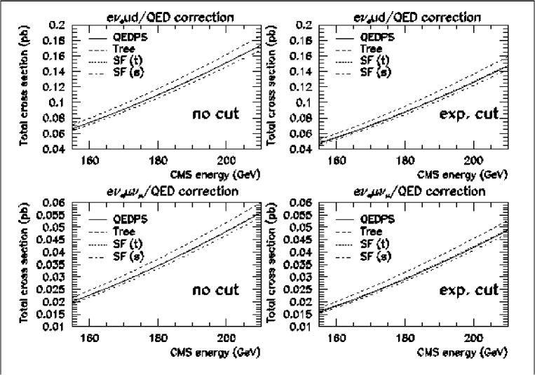
Figure 12.4: Total cross sections for $e\nu_{e}\bar{u}d$ and $e\nu_{e}\mu\nu_{\nu}$ processes without and with the experimental cuts described in the text. SF(t) denotes SF with correct energy scale and SF(s) with wrong energy scale ($s$).

In the JLC region, processes with more particles in the final state, such as $e^{+}e^{-}\rightarrow 6$ fermions become important because it is expected for the top-quark pair production. The experience at LEP-II tells us that one needs a generator equipped with the exact matrix elements that include all the diagrams that lead to the same 6-fermion final state, not only the ones via the resonant $t\bar{t}$ pair but also other non-resonant background diagrams. Already several activities appeared for this process: Montagna et al.[37] reported a full calculation of the 6-fermion process at $e^{+}e^{-}$ linear colliders, where the Higgs boson with an intermediate mass is produced, by the program package ALPHA[22] for the calculations of the matrix elements and HIGGSPV/WWGENPV[38] for Monte Carlo event generation. Accomando et al.[39] have been calculating a semi-leptonic process such as $e^{+}e^{-}\to b\bar{b}qq^{\prime}l\nu$ by program package PHACT[40].

In Ref.[41] the process $e^{+}e^{-}\rightarrow b\bar{b}u\bar{d}\mu\bar{\nu}_{\mu}$ is discussed, which has been calculated by means of the parallel GRACE combining the parallel BASES and PVM GRACE with MPI and the load balancing[42]. It shows scalability up to 16 processors. Among the total of 232 diagrams (in unitary gauge) of the process, the $t\bar{t}$ production diagrams are dominant over the others. We have divided the major background diagrams into three categories: the diagrams with $W^{+}W^{-}\gamma$ (hereafter $WW\gamma$), those with $W^{+}W^{-}Z$ (hereafter $WWZ$), and those with single-$t$ through $W^{+}W^{-}$ pair production (hereafter $tWW$).

The total cross sections with various sets of the diagrams in the CM energy range 340-500 GeV are plotted in Figs.12.5 a) and b), where the solid line is the numerical result of the total cross section with all the diagrams, while the dashed line is the result with only the dominant $t\bar{t}$ diagrams. Besides the result with all the diagrams and that with the $t\bar{t}$ diagrams alone, those with the $t\bar{t}$ and the major background diagrams are also shown for comparison. The dotted line in a) shows the result with the $t\bar{t}$ and $WW\gamma$ diagrams, while that in b) is with the $t\bar{t}$ and $WWZ$. The dot-dashed lines in a) and b) show the result with the $t\bar{t}$, $WW\gamma$, and $tWW$ diagrams and that with the $t\bar{t}$, $WWZ$, and $tWW$ diagrams, respectively. These results shown by dotted and dot-dashed lines include the interferences among the selected diagrams.

As shown in Fig.12.5, cross sections with both the $t\bar{t}$ and the major background diagrams show different behaviors from that with all the diagrams. Their difference is about 3% at $\sqrt{s}$ = 500 GeV. This means that the effect from the interference between $t\bar{t}$ and the rest of the diagrams except $WW\gamma$, $WWZ$, and $tWW$ is also non-negligible and important. The contribution from the background diagrams to the total cross section, ${(\sigma_{all}-\sigma_{t\bar{t}})}/{\sigma_{t\bar{t}}}$, is less than 5% in total above the $t\bar{t}$ threshold.

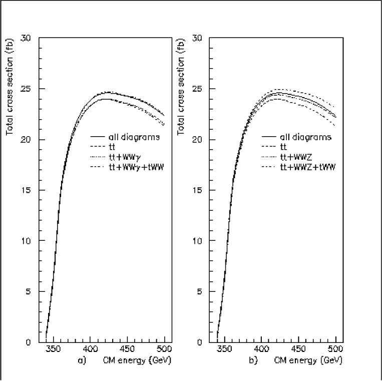
Figure 12.5: a) The total cross section with all the diagrams (solid line), with the $t\bar{t}$ diagrams alone (dashed line), with the $t\bar{t}$ and $WW\gamma$ (dotted line), and with the $t\bar{t}$, $WW\gamma$, and $tWW$ (dot-dashed line). b) The total cross section with all diagrams (solid line), with the $t\bar{t}$ diagrams alone (dashed line), with the $t\bar{t}$ and $WWZ$ (dotted line), and with the $t\bar{t}$, $WWZ$, and $tWW$ (dot-dashed line).

Generators for the MSSM

A lot of 2-to-2 reactions in the models beyond the SM are implemented in SPYTHIA and ISAJET. For precision measurements, however, we need generators with full matrix elements that lead to the same multi-body final states as expected for these 2-to-2 reactions after decays. In the MSSM, there appear 55 particles and 3,553 vertices. The number of Feynman diagrams for such a multi-body final state naturally becomes huge. Therefore, again, an automatic system plays important role. The generators for the processes $e^{+}e^{-}\rightarrow\tilde{\chi}_{1}^{+}\tilde{\chi}_{1}^{-}\rightarrow\tilde{\chi}_{1}^{0}\tilde{\chi}_{1}^{0}q\bar{q^{\prime}}q^{\prime\prime}\bar{q}^{\prime\prime\prime}$[43], and $e^{+}e^{-}\rightarrow\tilde{t}_{1}\tilde{t}_{1}^{*}H$[44] are available.

About 1-loop corrections, there exist only some calculations, no generator at this moment because calculations of the cross sections cost too much CPU time. In the full MSSM, the following one-loop corrections are available: $H^{+}\rightarrow t\bar{b}$[45], $e+e^{-}\rightarrow t\bar{t}$[46], $e+e^{-}\rightarrow W^{+}W^{-}$[11, 12], $e+e^{-}\rightarrow Z^{0}h^{0}$[47], and $e+e^{-}\rightarrow H^{+}H^{-}$[48]. For $e^{+}e^{-}\rightarrow\tilde{t}\tilde{t}^{*}$, 1-loop corrections in QCD-MSSM has been calculated[49].

Among the processes above, $e+e^{-}\rightarrow W^{+}W^{-}$ has a huge cross section in the JLC energy region and the deviation from the SM is important. For the analysis here, we use the following values for the input parameters:

$M_{Z}=91.1867$ GeV, $M_{W}=80.35$ GeV, $m_{t}=174$ GeV, $m_{b}=4.7$ GeV,

$m_{e}=0.51099906$ MeV, $m_{\mu}=105.658389$ MeV, $m_{\tau}=1.7771$ GeV,

$m_{u}=58$ MeV, $m_{d}=58$ MeV, $m_{s}=92$ MeV, $m_{c}=1.5$ GeV,

$\tan\beta=15$, $\mu=-300$ GeV, $M_{2}=200$ GeV,

$m_{\tilde{e}_{1}}=m_{\tilde{e}_{2}}=300$ GeV,  $\theta_{e}=0.1$,   $m_{\tilde{\nu_{e}}}=289.14$ GeV,

$m_{\tilde{\mu}_{1}}=m_{\tilde{\mu}_{2}}=300$ GeV,  $\theta_{\mu}=0.1$,   $m_{\tilde{\nu_{\mu}}}=289.14$ GeV,

$m_{\tilde{\tau}_{1}}=m_{\tilde{\tau}_{2}}=300$ GeV,  $\theta_{\tau}=0.1$,   $m_{\tilde{\nu_{\tau}}}=289.14$ GeV,

$m_{\tilde{u}_{1}}=m_{\tilde{u}_{2}}=m_{\tilde{d}_{1}}=300$ GeV,  $\theta_{u}=\theta_{d}=0.1$,   $m_{\tilde{d}_{2}}=396.25$ GeV,

$m_{\tilde{c}_{1}}=m_{\tilde{c}_{2}}=m_{\tilde{s}_{1}}=300$ GeV,  $\theta_{c}=\theta_{s}=0.1$,   $m_{\tilde{s}_{2}}=396.25$ GeV,

$m_{\tilde{t}_{1}}=200$ GeV,   $m_{\tilde{t}_{2}}=400$ GeV,   $m_{\tilde{b}_{1}}=200$ GeV,  $\theta_{t}=0.85,\theta_{b}=0.95$,   $m_{\tilde{b}_{2}}=221.8$ GeV.

$m_{h_{0}}=90.258$ GeV,   $m_{H_{0}}=250.337$ GeV,   $m_{H_{A}}=250$ GeV,   $m_{H_{\pm}}=262.595$ GeV,

$m_{\tilde{\chi}^{0}_{1}}=94.66$ GeV,   $m_{\tilde{\chi}^{0}_{2}}=184.23$ GeV,   $m_{\tilde{\chi}^{0}_{3}}=309.89$ GeV,   $m_{\tilde{\chi}^{0}_{4}}=326.97$ GeV,

$m_{\tilde{\chi}^{+}_{1}}=184.41$ GeV,   $m_{\tilde{\chi}^{+}_{2}}=330.01$ GeV,

This set was chosen based on the following criteria: 1) the value of $\tan\beta$ is not too small to have already been experimentally excluded, 2) the lighter chargino can be pair-produced at $\sqrt{s}=$500 GeV, 3) all sfermion masses are less than $\sim$ 1 TeV but heavier than 250 GeV, so that they are not pair-produced at $\sqrt{s}=500$ GeV, and 4) all the Higgs bosons except for the lighter CP-odd Higgs boson are not pair-produced at $\sqrt{s}=$500 GeV.

The result of the calculation has been confirmed through the following checks:

• The UV divergence is canceled among the 1-loop diagrams.

• The infrared divergence is canceled between the 1-loop diagrams and the soft photon corrections.

• The results are independent of the renormalization schemes [50] or [51] adopted in the computation.

Table 12.1: The total cross section at tree level $\sigma_{tree}$, $O(\alpha)$ corrected total cross sections in the SM($\sigma^{O(\alpha)}_{SM}$) and in the MSSM($\sigma^{O(\alpha)}_{MSSM}$), respectively, at $\sqrt{s}=$200 and 500GeV. $\delta$ shows the deviation of the MSSM results from the SM one in %. $k_{c}$ is set $0.05\sqrt{s}$.

$\sqrt{s}$(GeV)	$\sigma_{\mbox{tree}}$(pb)	$\sigma^{O(\alpha)}_{\mbox{SM}}$(pb)	$\sigma^{O(\alpha)}_{\mbox{MSSM}}$(pb)	$\delta(\%)$
200	18.001	15.928	15.785	$-$0.897
500	6.765	5.789	5.700	$-$1.69

The results are shown in Table 12.1. The soft photon cut parameter $k_{c}$ is set to $0.05\sqrt{s}$. For the set of the above input parameters, the deviation from the SM value is less than 1% in the LEP-II energy region, and still small at $\sqrt{s}=$500 GeV in the JLC energy region. Figs. 12.6 and 12.7 show the angular dependence of the differential cross sections with $k_{c}=0.05\sqrt{s}$ and of the deviation, $\delta$. The solid and dashed lines of the differential cross sections correspond to the MSSM case and to the SM case, respectively. At $\sqrt{s}=$200 GeV, the two curves are visually indistinguishable.

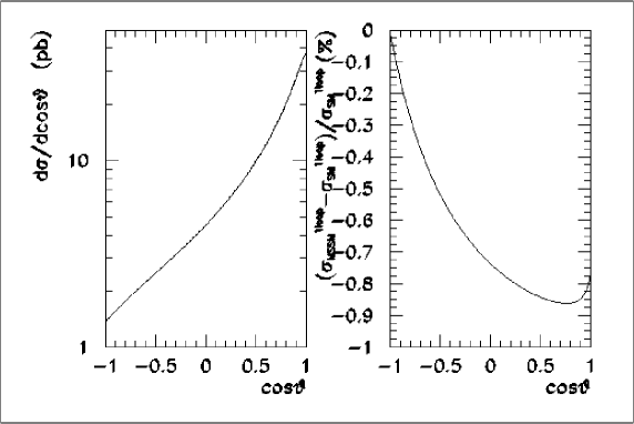
Figure 12.6: $O(\alpha)$ corrected $d\sigma/d\cos\theta$ in the SM(the dashed line) and in the MSSM(the solid line) and the deviation $\delta$ in % at $\sqrt{s}=$200 GeV with $k_{c}=0.05\sqrt{s}$.

On the other hand, at $\sqrt{s}=$500 GeV GeV, the deviation becomes large in the backward region. It might not be, however, so easy to see it in real experiments because of its small cross sections in that angular region.

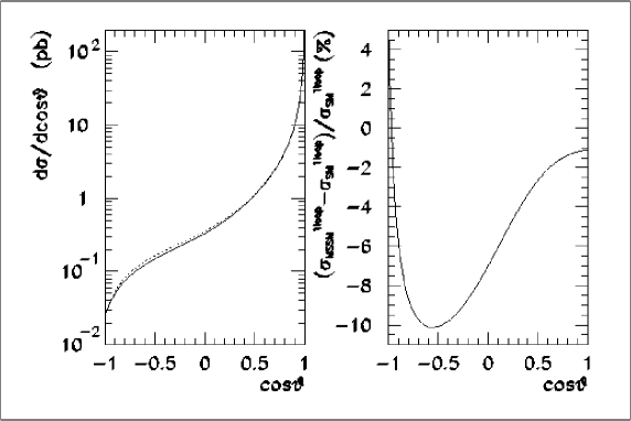
Figure 12.7: $O(\alpha)$ corrected $d\sigma/d\cos\theta$ in the SM(the dashed line) and in the MSSM(the solid line) and the deviation $\delta$ in % at $\sqrt{s}=$500 GeV with $k_{c}=0.05\sqrt{s}$.

Fig.12.8 shows the energy dependence of the deviation $\delta$ with the above set of the input parameters. Up to $\sqrt{s}=$1000 GeV, the deviation stays small and is less than around 3%.

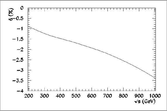
Figure 12.8: The center of mass energy dependence of the deviation $\delta$ in % with $k_{c}=0.05\sqrt{s}$.

12.4 Detector Simulators

12.4.1 QuickSim: a Fast Simulator

There are two approaches to quick simulations. The first approach that is adopted for tracking part of the JSF relies on calculations of various error matrices. Consider a track parameter vector (${\bf a}$) and its error matrix ($E_{\bf a}$). Linearization reduces the $\chi^{2}$ of its measurement into a parabolic form:

$$\chi^{2}=\frac{1}{2}\Delta{\bf a}^{T}\cdot E_{\bf a}^{-1}\cdot\Delta{\bf a}.$$ (12.5)

Being symmetric, $E_{\bf a}$ can be diagonalized using an orthogonal matrix $O$ as

$$E_{\bf b}^{-1}=O^{T}\cdot E_{\bf a}\cdot O=\left(\begin{array}[]{ccc}1/\sigma_{1}^{2}&{}\hfil&0\cr{}\hfil&\ddots&{}\hfil\cr 0&{}\hfil&1/\sigma_{n}^{2}\end{array}\right).$$ (12.6)

Using this, we can rewrite the $\chi^{2}$ as

$$\chi^{2}=\frac{1}{2}\Delta{\bf b}^{T}\cdot E_{\bf b}^{-1}\cdot\Delta{\bf b},$$ (12.7)

where $\Delta{\bf b}$ is defined by

$$\Delta{\bf b}=O^{T}\cdot\Delta{\bf a}.$$ (12.8)

Since the components of $\Delta{\bf b}$ are independent, we can now smear them as

$$\Delta{\rm b}_{i}=\sigma_{i}\cdot(\mbox{Gaussian random number with unit width})$$ (12.9)

from which we can obtain a smeared ${\bf a}$ as

$${\bf a}={\bf a}_{\rm true}+O\cdot\Delta{\bf b}.$$ (12.10)

Notice that in this way it is possible to properly take into account any correlation among components of the original parameter vector ${\bf a}$. Since one can approximately calculate error matrices, knowing basic detector parameters such as geometry and resolutions, this approach is useful to see how the overall detector performance varies with these basic parameters.

The second approach is based on a parametric smearing and is more empirical and practical, which is used for calorimetry. Smearing parameters are tuned to reproduce results from corresponding full simulators, and, once tuned, the simulation can be quick and fairly accurate. This approach is therefore useful for physics simulations that require high statistics.

Components we have in the Quick Simulator are as follows: a beam pipe, Vertex Detector (VTX), Intermediate Tracker (IT), Support Tube, Central Drift Chamber (CDC), Electromagnetic (EM) and Hadron (HD) Calorimeters. Parameters of them, such as the number of layers, thickness, resolution, etc. are all controlled by input cards.

In QuickSim, charged particle smearing goes as follows.

1. A particle information is obtained from generator data and a track starts.

2. The track is swum in the magnetic field towards the beam pipe and, if it reaches there, its direction gets smeared due to multiple scattering.

3. The track is further swum to the inner-most VTX layer, and its direction gets smeared again by multiple scattering.

4. From the position and momentum of the track at the inner-most layer of VTX, a VTX track parameter vector is formed and smeared by the error matrix method as described above.

5. The track is then swum to the next VTX layer and its direction is smeared again due to multiple scattering. This procedure is repeated all the way through the rest of the VTX layers, all of the IT layers, and the support tube to the inner-most sense-wire layer of CDC.

6. From the position and momentum of the track at the inner-most CDC layer, a CDC track parameter vector is calculated and smeared with the error matrix method.

7. The track is further swum to the calorimeter and creates cell signals. Electrons leave signals in the EM section and hadrons in the HD section of the calorimeter. Currently, muons do not generate signals in the calorimeter.

8. The pivot of the CDC track parameter vector is moved back to that of the VTX track parameter vector taking into account the effects of multiple scattering on the error matrix. They are then averaged to get a combined VTX-CDC track parameter vector.

The energy loss of particles is not considered in QuickSim.

The smearing of neutral particles is more straight-forward as we just extrapolate them to the calorimeter and generate smeared signals. To simulate the effects of the lateral spread of the calorimeter signals, a projected shower distribution given by,

$$f(x)=a_{1}e^{-|x|/\lambda_{1}}+a_{2}e^{-|x|/\lambda_{2}}.$$ (12.11)

is used, where $a_{i}$ and $\lambda_{1}(i=1,2)$ are tunable parameters for shower shape. The energy deposit in each of the hit cells is calculated by integrating this distribution over the cell size.

To use the calorimeter signals for physics analysis, the signals distributed to cells have to be clustered, which is done in QuickSim. The algorithm we adopted to cluster EM calorimeter signals is as follows:

1. Find the highest energy cell BL1 among those with an energy larger than ETH.

2. Attach neighbor cells BL2 to the seed cell BL1.

3. Check BL3 that is a neighbor cell of BL2 and include it in the cluster if one of the following two conditions is satisfied:

   • $E(BL2)>c1\times E(BL1)$

   • $E(BL3)>c2\times E(BL1)\;\mbox{~{}and~{}}\;E(BL3)<c3\times E(BL2)$,

   where $c1$, $c2$, and $c3$ are parameters to be optimized, depending on the calorimeter geometry.

In order to optimize the clustering parameters, we generated a single photon or two photons with a fixed opening angle but with a varying energy between 1 GeV to 50 GeV, and tuned the parameters so that the number of reconstructed photons matches the generated one. The opening angle of the photons in the case of the two-photon generation is fixed at 30mrad, 50mrad, and 100mrad. The clustering efficiencies are shown in Fig. 12.9 as a function of the parameters.

    

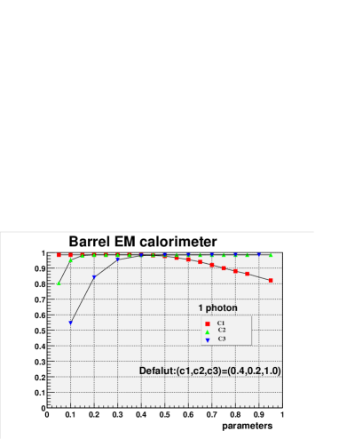
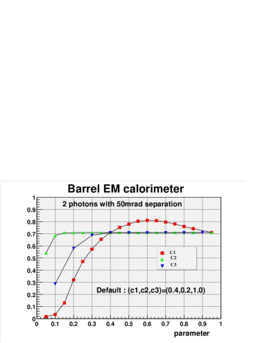
a)                                                            b)

Figure 12.9: The efficiency to cluster (a) a single photon as a single photon, and (b) two photons as two photons. The photon energy is varied from 1 GeV to 50 GeV, randomly, while the opening angle in the case of two-photon generation is fixed at 50 mrad, while their directions are randomly varied among Barrel calorimeter region. Red squares, green up, and blue down triangles are efficiencies when only $c1$ or $c2$ or $c3$ is modified, respectively.

A charged track is flagged as muon or electron with the help of generator information. If there is no electron matched with an EM cluster, it is considered as a photon cluster. The cluster-track matching is performed based on their position and energy differences. If a track and an EM cluster match in position but differ in energy by more than 2-$\sigma$ of their resolutions, the energy excess in the EM cluster is attributed to a photon cluster overlapping with the electron cluster.

In the case of the HD clusters, we used a method to link multiple tracks to a connected set of HD cells, instead of relying on clustering using the HD section alone[7]. In this method, we first form a connected set, called an island hereafter, of hit HD cells without trying to separate multiple peaks within the island. Charged tracks are then extrapolated to the island. If the sum of the track energies matches with the total energy deposit in the island within $2\sigma$ of the calorimeter resolution, the island is simply deleted and each of the matched tracks are flagged as a combined track from a purely charged particle. If they differ by more than $2\sigma$, we subtract the track energies from the energy deposit in the island and attribute the excess to a possible neutral hadron. Each of the tracks that matched in position with the island is then flagged as a charged hadron in a mixed HD cluster.

Results of the cluster-track matching are stored in a class called JSFLTKCLTrack, which serves as a starting point of the most of physics analyses.

12.4.2 JIM and JLCSIM: a Full Simulator

As for full simulators, we have to implement materials and physics processes as realistic as possible, since their primary usage is to check the validity of the corresponding quick simulators. JIM is a GEANT3-based full detector simulator being developed for this purpose and is distributed as the JLCSIM package together with utilities to analyze JIM data. It includes two versions of geometry models: one for 2 Tesla magnetic field[17] and the other for 3 Tesla. The 3 Tesla model was introduced recently to accommodate a higher luminosity. The geometry of the 3 Tesla model is shown in Fig.12.10. In both models, realistic shapes of the detector and structural components are implemented with the exception of the 3-Tesla version of CDC and the Intermediate Tracker in both models. Geometry components and its status are summarized in Table. 12.2.

Table 12.2: Detector components and its status defined in JIM.

Name	2-Tesla	3-Tesla
Central Tracker	Full	Cylinder
Intermediate Tracker	Cylinder	Cylinder
Calorimeters	Full	Full
Vertex	Full	Full and Cylinder
Muon	Full	Full
Mask and beam pipe	Full	Full
Magnet and return yokes	Full	Full

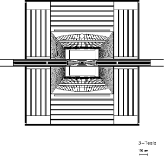
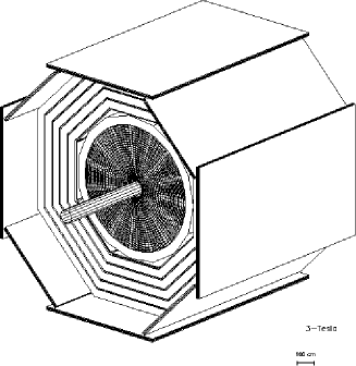
Figure 12.10: The JLC detector geometry of 3 Tesla model. The End Cap Muon system and Calorimeters are removed in the 3-D view to show the structure inside.

Hit positions of trackers created by JIM are exact hit information of particles and their smearing is performed by the analysis routines provided by JLCSIM. There are also programs for tracking and clustering, results of them are stored as a ntuple file with a format that is the same as with QuickSim. When JIM data are analyzed by the JSF, the JSF calls these utilities to store their data as instances of the objects in the JSF.

12.4.3 Comparison of QuickSim and JIM

Since QuickSim is an independent program of JIM, their performances are compared in terms of momentum resolution, impact parameter resolution, and calorimeter resolution, for the case of the 3 Tesla detector parameters.

To compare the momentum resolution, we generate a single muon track at 90^∘ with various momenta and the momentum resolution with and without VTX constraint are compared. Since the CDC geometry in JIM is an idealized cylindrical one, momentum resolutions of QuickSim and JIM should be essentially the same except for the effect of the ionization energy loss and large angle multiple scattering both of which are not considered in QuickSim.

To get the reconstructed momentum of each CDC track simulated by JIM, we made a five-parameter helix fitting to the CDC hit points. There are materials of 5% radiation lengths in front of CDC, which causes energy loss of about 2 MeV for a 10 GeV muon. When the momentum resolution of CDC is compared, this shift is ignored. For the combined track fitting, however, this shift cannot be neglected especially in the low momentum region. For the CDC-VTX combined track fitting of JIM data, we shift the momentum by amount of the average energy loss and the error matrix of the helix parameters is enlarged to include the effect of multiple scattering. The so obtained CDC helix parameter vector is then averaged with the corresponding VTX helix parameter vector. Resolutions are compared as a function of the track momentum in Fig. 12.11, which shows good agreement both in the cases of CDC only and CDC+VTX average. In the momentum region below 1 GeV, the resolution of JIM is better than QuickSim. At low momenta, tracks curl up in CDC volume and produces a large number of hit points. In QuickSim, the number of CDC hits are, however, restricted to the number of wires hit by the first radial segment for conservative simulation, while in JIM this restriction is absent. The better performance of JIM in the low momentum region can be attributed to this difference, but further verification is necessary.

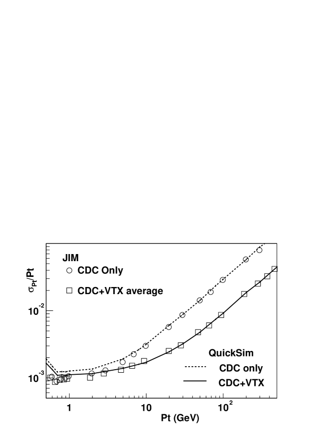
Figure 12.11: Momentum resolutions obtained by QuickSim and JIM.

The 2-D impact parameter resolutions are also compared between QuickSim and JIM in Fig. 12.12, showing good agreement.

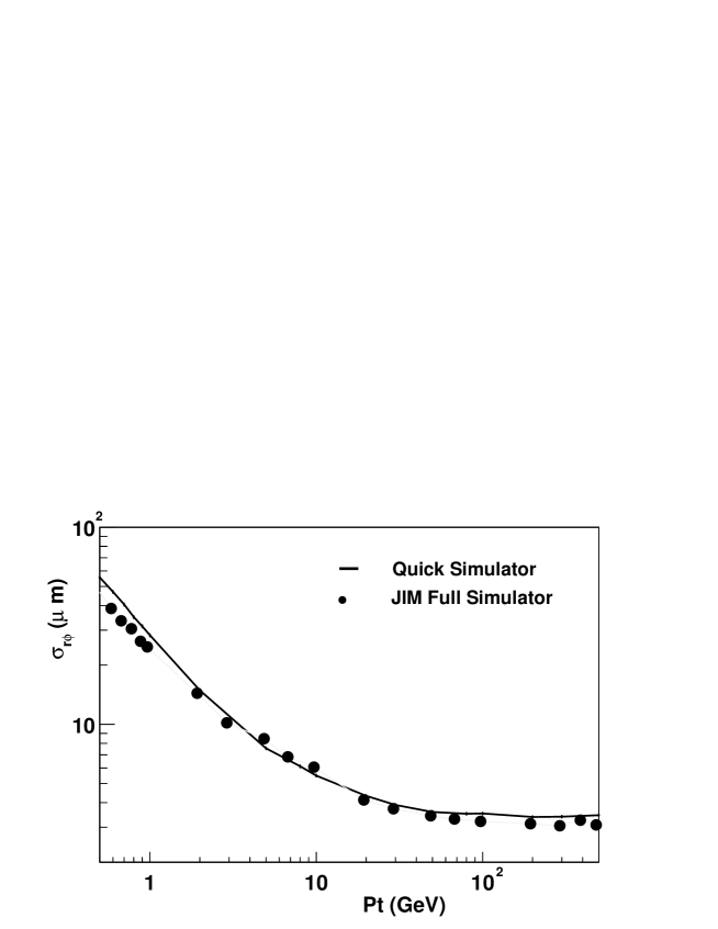
Figure 12.12: 2-D impact parameter resolutions obtained by QuickSim and JIM.

The energy resolutions of the calorimeter as simulated by QuickSim and JIM are compared in Fig. 12.13 for 10 GeV electrons and pions. The energy resolutions for the the electrons are mutually consistent, but that for the pions in JIM is larger than the QuickSim result. The energy resolution of the hadron calorimeter in JIM is even worse than beam test results, which suggests necessity of further tuning of the calorimeter simulation in JIM.

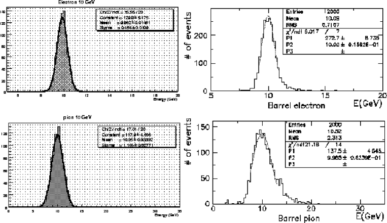
Figure 12.13: The energy distribution of calorimeter by QuickSim compared with that of JIM.

12.4.4 JUPITER : a GEANT4-based Simulator

As a new approach to full detector simulation, we are developing a GEANT4-based detector simulator called JUPITER (JLC Unified Particle Interaction and Tracking EmulatoR). One of the design goals of JUPITER is to allow easy modification of geometrical parameters that describe various detector components, since its currently conceived most important usage is to optimize the detector parameters for the JLC. To this end, we decided to organize base classes of JUPITER to mimic detector building process: assembling of each device and its subsequent installation, thereby facilitating easy replacement, uninstallation and reinstallation, of any detector component. In our design, every geometrical component, even the World Volume, must be a derived class from a base class called J4VDetectorComponent. This pure virtual base class specifies basic interfaces that any detector component must be equipped with: an Assemble() method to define a shape and material of the object as a G4Solid and a G4LogicalVolume, an InstallIn() method to install it into its mother volume, thereby appending positional information to the object as a G4VPhysicalVolume. The base class also provides an automatic naming system for the hierarchy of the detector components as well as some handy interfaces to frequently used shapes including tubes. For parallel and distributed development of various detector components, JUPITER also provides a base class called J4VMaterialStore for material definitions. By instantiating a class object derived from this base class, a developer of each detector component can define materials without conflicting with developers of the other parts.

Using these classes, we started with the development of the CDC part of JUPITER, which can now handle multi-particle final states as from the process $e^{+}e^{-}\rightarrow ZH$. A sample event display is shown in Fig.12.14 for this process generated at $\sqrt{s}=300$ GeV.

Figure 12.14: Event display of $e^{+}e^{-}\rightarrow ZH$ at $\sqrt{s}=300$ GeV simulated by JUPITER. Only charged tracks are shown.

The implementation of the VTX detector has begun recently, but those of the other detector components, not to mention the analysis packages for simulated data, are yet to be developed. It should also be noted that the validity of GEANT4 itself should be checked out, which needs dedicated studies.

12.5 Future Direction

As was mentioned in 12.2, the current JSF system uses, as its part of core libraries, legacy software packages written mainly in FORTRAN. One such example is the helicity amplitude subroutine package (HELAS) and differential cross section functions composed with HELAS. We are planning to develop a C++ version of HELAS (HELAS++) to facilitate object-oriented implementation of event generators. Another example is the detector simulators: a substantial part of our fast detector simulator QuickSim and essentially all of our GEANT3-based full simulator JIM are written in FORTRAN. We are now developing a new detector simulation system (JUPITER) based on GEANT4.

Part IV Options

Chapter 13 $\gamma\gamma$, $e^{-}\gamma$, $e^{-}e^{-}$

13.1 Introduction

At the time of its operation, the $e^{+}e^{-}$  linear collider will be source of the highest energy and the most intense electron beams. Using these electron beams, it is also possible to construct facilities to study high energy interactions other than the $e^{+}e^{-}$  collisions.

The simplest case is an $e^{-}e^{-}$  interaction which is realized by just replacing the positron beam with the electron beam. The other possibility is to convert the electron beam to the photon beam by the backward Compton scattering, providing facilities of the $\gamma\gamma$  interaction and/or the $e\gamma$  interaction.

In the JLC working group, feasibility of these ’optional’ interaction has been studied and the activity was mainly focused on the $\gamma\gamma$  and the $e\gamma$  interactions. A summary of the recent study was published as a KEK Report[1]. The activities are also found in the North America and the European LC working group and their recent works were described in refereces[1, 2, 3, 4].

As results of these studies, the overall picture of the physics opportunities with the options is fairly understood and we see many interesting and important subjects to be explored with them. They have potential to give an additional view or to give a complementary information to the $e^{+}e^{-}$  interactions. Therefore, full understanding the feasibility of the $\gamma\gamma$ , $e\gamma$ , and $e^{-}e^{-}$interactions both in physics and in technical aspects are important as a part of the linear accelerator project.

On the other hand, since the linear collider communities have paid their attention mainly to the $e^{+}e^{-}$collision so far, the understanding of the feasibility of these optional interaction is not the same level as those in the $e^{+}e^{-}$  interaction.

This chapter aims to describe overall view of the optional interaction mainly of $\gamma\gamma$  and $e\gamma$  interaction with the current knowledge, i.e,

• Overview of the $\gamma\gamma$  and $e\gamma$  interaction.

• Machine parameters and luminosities

• Physics opportunities

• Technical issues

• Future prospects

13.2 $\gamma\gamma$  and $e\gamma$  Collider

The JLC accelerator scheme with the second interaction region is illustrated in Fig. 13.1.

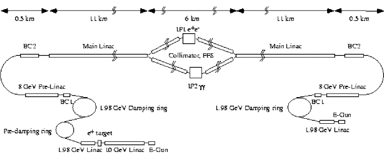
Figure 13.1: Schemtic of the JLC with the second interaction region.

In the $\gamma\gamma$  and the $e\gamma$  colliders, photon beams are generated by the backward Compton scattering of electron- and laser-beams just before the interaction point. The maximum energy of the generated photon is expressed as;

$$E_{\gamma}\big{|}^{max}={x\over{x+1}}E_{e}.$$ (13.1)

Here, $x$ is a kinematics parameter of the Compton scattering, defined as

$$x={{4E_{e}\omega_{L}}\over{m_{e}^{2}}}\cos^{2}(\theta/2),$$ (13.2)

where $E_{e}$, $\omega_{L}$ and $\theta$ are the electron energy, laser photon energy and angle between the electron beam and the laser beam (see Fig. 13.2).

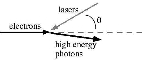
Figure 13.2: Kinematics of inverse-Compton scattering.

A calculated photon energy spectrum generated by the backward Compton scattering is shown in Fig. 13.3.

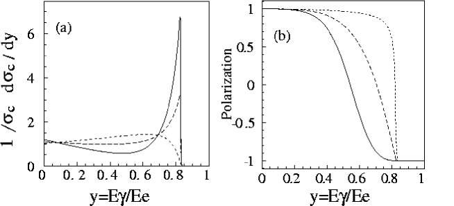
Figure 13.3: Calculated energy and polarization of back-scattered photons by laser-Compton scattering for different combination of the laser and the electron beam polarization, i.e., $P_{L}P_{e}=-1$ (solid), $P_{L}P_{e}=0$ (dashed) and $P_{L}P_{e}=1$ (dotted), respectively.

As seen from the figure, energy distribution of the photon depends on the polarization of the electron and the laser beam, i.e., one can obtain a broad energy distribution or peaked distribution by controlling the polarization.

According to equation (13.1), the maximum photon energy increases as $x$ becomes higher. However, when $x$ exceeds $2(1+\sqrt{2})\approx 4.83$, the energy of a Compton-scattered photon and a laser photon system exceeds the threshold of $e^{+}e^{-}$pair creation. This pair-creation process could waste generated high-energy photons and could be an additional source of detector background so that, at least as a first assumption, $x$ parameter is restricted to be smaller than 4.83, corresponding to the maximum photon energy of about 80% of the electron energy.

Since a precise estimation of the luminosity of $\gamma\gamma$ colliders requires a detail consideration of the laser-Compton scattering and geometry of the interaction region, which need a simulation of the laser-Compton scattering as well as beam-beam interaction, we estimate here the luminosity of $\gamma\gamma$ colliders by a simple analysis. With the typical parameters of the photon collider, the Compton-conversion probability for an electron, i.e., mean number of Compton interactions of an electron in a laser pulse, is assumed to be 1. With this assumption, the conversion efficiency $k$, is calculated as;

$$k=\sum\limits_{n=1}^{\infty}{P_{n}^{1}=1-e^{-1}}\approx 0.63$$ (13.3)

where $P_{n}^{1}$ is a probability that an electron encounters $n$ laser photons when its average is 1. Thus the number of scattered photons ($N_{\gamma}$) is $0.63N$, with $N$ being the number of electrons in a bunch. Usually, we are interested in the high energy part of the spectrum and if we take high energy part ($E_{\gamma}>65\%$) of the spectrum, the effective conversion efficiency $k^{\prime}$ can be regarded as $k^{\prime}\approx 0.3$.

The photon beam spot size at the interaction point is more or less same as that of the electron beam since the scattered photons are boosted toward the electron beam direction. Particularly, spot size of the high energy part can be assumed to be the same as the electron beam. Therefore, the luminosity of the $\gamma\gamma$ collider is expressed approximately as;

$$L_{\gamma\gamma}=k^{\prime 2}L_{ee}\approx 0.3^{2}L_{ee}\approx 0.1L_{ee},$$ (13.4)

where $L_{ee}$ is the geometric luminosity of $e^{-}e^{-}$ collisions defined as;

$$L_{ee}={{N^{2}f}\over{4\pi\sigma_{x}^{e}\sigma_{y}^{e}}}$$ (13.5)

with $N$, $f$, $\sigma_{x}^{e}$, $\sigma_{x}^{e}$ and $\sigma_{x}^{e}$ being the number of electrons in a bunch, the bunch repetition, the horizontal and the vertical bunch size at the interaction point, respectively. It should be noted that the geometric luminosity is not necessary to be the same as the $e^{+}e^{-}$collider. Since the effect of the beam beam interaction is less serious then $e^{+}e^{-}$ interaction, the geometric luminosity is possibly higher that the $e^{+}e^{-}$collision.

More precise estimation of the luminosity spectrum can be performed using numerical simulation with a specific parameters of the electron and the laser beam. As an example, the parameters for the JLC $\gamma\gamma$ collider is shown in table 13.1.

Table 13.1: Major parameters of $\gamma\gamma$  collisions at JLC-I.

Parameter set			(a)	(b)	(c)
$e^{-}$
Beam energy	$E_{e}$	GeV	250	103	80
Particles/bunch	$N$		0.95$\times 10^{10}$	$\leftarrow$	$\leftarrow$
Repetition rate	$f_{rep}$	Hz	150	$\leftarrow$	$\leftarrow$
bunches/pulse	$n_{b}$		95	$\leftarrow$	$\leftarrow$
Bunch length	$\sigma_{z}$	$\mu$m	120	$\leftarrow$	$\leftarrow$
Bunch sizes at IP	$\sigma_{x}^{*}/\sigma_{y}^{*}$	nm	680/12.8	77/12.2	88/10.7
Beta func. at IP	$\beta_{x}^{*}/\beta_{y}^{*}$	mm	0.5/0.8	0.3/0.5	0.3/0.3
Norm. emittance	$\varepsilon_{xn}/\varepsilon_{yn}$	nm$\cdot$r	4500/100	4000/60	$\leftarrow$
Vertical offset		$\sigma_{y}^{*}$	1	$\leftarrow$	$\leftarrow$
CP-IP distance	$d$	mm	7.0	3.3	2.8
Geom. luminosity	L${}^{ee}_{geom.}$	cm-2s-1	11.8$\times 10^{33}$	6.78$\times 10^{33}$	6.79$\times 10^{33}$
Laser
Wave length	$\lambda_{L}$	$\mu$m	1.053	$\leftarrow$	0.37
Pulse energy	$E_{L}$	J	1.0	$\leftarrow$	$\leftarrow$
Pulse length	$\sigma_{z}^{L}$	$\mu$m	230	$\leftarrow$	120
r.m.s spot size	$\sigma_{0}^{L}$	$\mu$m	3.17	$\leftarrow$	1.53
$x$ parameter	$4\omega_{L}E_{e}/m_{e}^{2}$		4.51	1.86	4.11

Parameter sets are one for the high energy operation with 250 GeV electron beam and two for low energy operation. Difference of two parameter sets for low energy operation is the wave length of the laser, i.e., one with $1\mu m$ and one with $0.37\mu m$. For both case, the maximum photon energy is set at 60 GeV with 120 GeV Higgs boson in mind.

The luminosity distributions simulated using CAIN[5], a simulation program for the laser-electron and the beam-beam interaction, for the high energy operation is shown in Fig. 13.4.

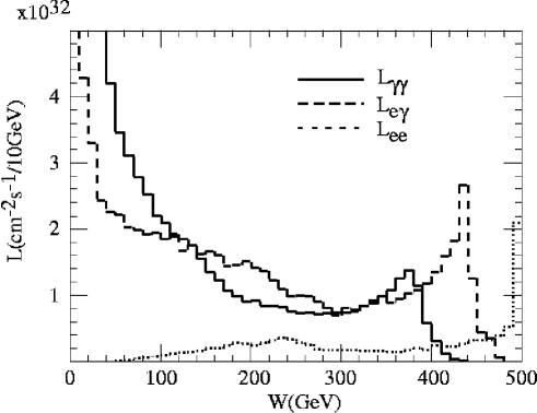
Figure 13.4: Luminosity distributions simulated by CAIN for collisions, the solid, dashed and dotted lines are luminosities of $\gamma\gamma$ , $e\gamma$  and $e^{-}e^{-}$ collisions, respectively, and $W$ is their center-of-mass energies.

We have $\gamma\gamma$, $e\gamma$  and $e^{-}e^{-}$  interaction simultaneously as well as low energy interaction caused by beamstrahlung photons.

The other feature of the $\gamma\gamma$ interaction is that it is possible prepare polarized photon beam both circularly and linearly. For example, the Higgs bosons are produced with the $J_{z}=0$ combination of the initial photons while the background process as $\gamma\gamma\to f\bar{f}$ are suppressed with this helicity configuration.

It is also pointed out that the linearly polarized photon beam is useful to investigate CP nature of the Higgs boson [6, 7, 8, 9, 10]. Fig. 13.5 shows luminosity distribution (CAIN simulation) when parameters are set for linearly polarized photons.(see 13.3.1)

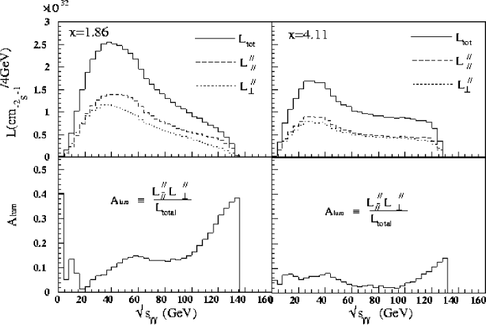
Figure 13.5: Linearly polarized luminosities(top) and the asymmetries(bottom) at 120-GeV $\gamma\gamma$  collisions, which are simulated by CAIN, where $L^{\parallel}_{\parallel}$(dashed), $L^{\parallel}_{\perp}$ (dotted) and $L_{\rm{total}}\equiv L^{\parallel}_{\parallel}+L^{\parallel}_{\perp}$(solid). The left and right figures correspond to the parameter sets of (b) and (c) in table 13.1, respectively.

13.2.1 $e\gamma$ Collider

The $e\gamma$ collider mode can be obtained by turning off the laser for one side at the $\gamma\gamma$ collider operation. If we use the same discussion on the luminosity of the $\gamma\gamma$ collider, the luminosity of the high energy part of the $e\gamma$ luminosity distribution can be estimated as;

$$L_{e\gamma}=k^{\prime}L_{ee}\approx 0.3L_{ee}.$$ (13.6)

The result of the of numerical simulation is shown in Fig.13.6.

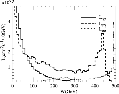
Figure 13.6: Luminosity distributions for $e\gamma$  collider mode simulated by CAIN, where the solid, dashed and dotted lines are luminosities of $\gamma\gamma$,  $e\gamma$  and $e^{-}e^{-}$  collisions, respectively, and $\sqrt{s}$ is their center-of-mass energies.

13.2.2 $e^{-}e^{-}$Collider

The collision of the same sign beam suffers from the anti-pinch effect due to the repulsive force between them. It requires a careful tuning of the beam parameters because, small beam size increases the beamstrahlung but may not gain the luminosity. The discussion on the optimization of the luminosity of the $e^{-}e^{-}$collider is found in ref. [11]. According to the discussion, the typical luminosity of the $e^{-}e^{-}$  collider is around 30% of the $e^{+}e^{-}$collider. A simulated luminosity distribution is show in Fig.13.7.

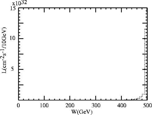
Figure 13.7: Luminosity distributions for $e^{-}e^{-}$  collider mode simulated by CAIN

As an example of the parameter, a parameter set for JLC/NLC (ISG-B)[12] $e^{+}e^{-}$ collider were used with replacing a positron beam to the electrons. In this particular case, the luminosity was about 20% of the those of the $e^{+}e^{-}$ luminosity with the same parameters.

13.2.3 Summary of the luminosities

The summary of typical luminosity of $\gamma\gamma$,  $e\gamma$,  and $e^{-}e^{-}$collider is shown in table 13.2.

Table 13.2: Summary of luminosities of various LC options based on the JLC parameters.

Luminosity in $\times 10^{33}$ cm-2s-1	$\gamma\gamma$(a)	$\gamma\gamma$(b)	$\gamma\gamma$(c)	$e\gamma$	$e^{-}e^{-}$
$e^{-}-e^{-}$ geometric	11.8	6.8	6.8	11.8	6.3
$\gamma-\gamma$ total	10.5	9.3	5.3	5.5	N/A
$\gamma-\gamma$ [eff]	1.4	1.6	1.0	0	N/A
$e^{-}-e^{-}$ total	1.3	0.5	0.4	1.2	1.4
$e^{-}-e^{-}$ [eff]	0.9	0.4	0.2	1.0	1.4
$e-\gamma$ total	8.1	5.1	3.4	6.8	N/A
$e-\gamma$ [eff]	2.5	2.1	1.1	2.3	N/A

Roughly speaking, typical luminosity of the options are:

• $L_{\gamma\gamma}^{eff}\approx 0.1L_{geom}^{e^{-}e^{-}}$

• $L_{e\gamma}^{eff}\approx 0.3L_{geom}^{e^{-}e^{-}}$

• $L_{e\gamma}^{eff}\approx 0.3L^{e^{+}e^{-}}$

It has to be noted that the optimization of these luminosities are still possible and we could expect higher luminosity without major change in accelerator parameters. More detail discussion on the optimization can be found in [11, 13].

13.3 Physics

13.3.1 Higgs Bosons

The search for and study of the Higgs boson, the last missing member of the standard model family, are among the most important tasks for future colliders, such as the Large Hadron Collider (LHC) and $e^{+}e^{-}$linear colliders.

The interaction of high-energy photons at a $\gamma\gamma$  collider [14, 15, 16, 17, 18, 19, 1, 20] provides an opportunity to study the Higgs boson. As described later, the number of events expected in the $\gamma\gamma$  interaction is expected to be 5000 per 10fb^-1 for a Higgs boson of 120GeV, while it is approximately 1000 per 10fb^-1 in an $e^{+}e^{-}$collision. The Higgs-boson physics at the $\gamma\gamma$  collider has been studied by several authors, and it has been shown that studies of the intermediate-mass Higgs in the mass region $M_{W}<M_{H}<2M_{W}$ through the $\gamma\gamma\to H\to b\bar{b}$ process is complementary to an $e^{+}e^{-}$ linear collider or a hadron collider, such as study of the CP property, or exploring physics beyond the standard model through measurements of the two-photon decay width [21, 22, 24, 25, 26, 27, 28, 29, 30, 2].

Figure 13.8 shows a schematic diagram of the coupling of the Higgs boson to two photons. Since two photons do not directly couple to the Higgs boson, but do only through a loop diagram of massive charged particles, any kind of massive charged particles contributes to the two-photon decay width of the Higgs boson [31, 32]. In the standard model, the dominant contributions come from the top and W-boson loop. It should be noted that since the contribution of bosons and fermions in the loop interfere destructively, it is expected to observe this destructive interference between the top and W-boson loop for the Higgs of 500-700 GeV. If the gauge coupling of the Higgs and W boson is measured in the $e^{+}e^{-}$interaction with good precision, a measurement of the two-photon decay width of the Higgs boson could provide an information concerning the Yukawa coupling of the Higgs boson and the top quark.

Regarding physics beyond the standard model, a deviation of the two-photon width from the standard model prediction indicates an additional contribution from unknown particles, and is a signature of physics beyond the standard model. For example, the supersymmetric extension of the standard model (MSSM) has additional charged particles, such as scalar fermions, charged Higgs bosons and charginos. Since the masses of these particles partly originate from the Higgs mechanism of the electroweak symmetry breaking, the presence of theses particles results in a shift of the two-photon decay amplitude of the Higgs boson from its value of the SM. In fact, a minimal extension of the standard model(MSSM) predicts the ratio of two-photon decay widths ($\Gamma(h^{0}\to\gamma\gamma,\mbox{MSSM})/\Gamma(H\to\gamma\gamma,\mbox{SM})$) to be as much as 1.2 for the lightest Higgs boson having a mass of 120 GeV Higgs [22].

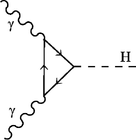
Figure 13.8: Coupling of the Higgs boson to two photons.

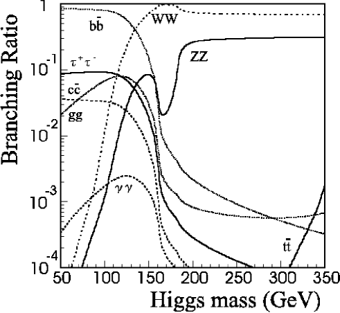
Figure 13.9: Branching ratios for the standard model Higgs boson for a 176-GeV top-quark mass.

SM Higgs Boson

The intermediate-mass Higgs boson in the SM mainly decays into a $b\bar{b}$ pair, as is shown in Fig. 13.9, and the daughter b-flavored hadrons will be easily identified due to their long lifetime; therefore, $b\bar{b}$ events are the best signal of the intermediate-mass Higgs bosons. Although the main background may be the continuum $\gamma\gamma\to q\bar{q}$ processes, the background events are dominantly produced by the initial photon collision in the $J_{z}=\rm 2$ angular momentum state, and it can be suppressed by controlling the polarization of the colliding photon beams. Simultaneously, beam polarization enhances the Higgs boson signals, which are only accessible by the $J_{z}=0$ collisions [23, 22]. The feasibility of a measurement of the two-photon decay width of the Higgs boson in this mass region has been studied by Borden et al.[21, 24].

Recently, several authors reported that the effect of QCD corrections to $\gamma\gamma\to q\bar{q}$ is large, since the helicity suppression in the $J_{z}=0$ channel does not work due to gluon emission. It could be a serious source of background in the intermediate-mass Higgs boson detection, since some of the three-jet events from the $J_{z}=0$ state may mimic two-jet events [24, 29, 30].

In this work, we simulate a measurement of the two-photon decay width of the Higgs boson with a mass of 120 GeV at a $\gamma\gamma$  collider, including the effect of QCD correction for the $\gamma\gamma\to q\bar{q}$ process in the manner of Jikia and Tkabladze [30]. To perform a realistic evaluation, the Monte-Carlo programs CAIN[33, 34, 5], JETSET7.3[37] and JLC-I detector simulator[39] were applied to find the luminosity distribution of a $\gamma\gamma$  collider, hadronization and selection performance in the detector, respectively.

Assuming the Higgs boson mass of 120 GeV, a set of parameters suitable for a study was prepared, as listed in tabel 13.3.

Electron beam parameters
Number of electrons per bunch	$N_{e}$	$0.63\times 10^{10}$
Number of bunches per pulse	$n_{b}$	85
Repetition rate	$f_{rep}$	150	Hz
Normalized emittance	$\gamma\epsilon_{x,e}$	$3.3\times 10^{-6}$	m
	$\gamma\epsilon_{y,e}$	$4.8\times 10^{-8}$	m
R.m.s. bunch length	$\sigma_{z,e}$	90	$\mu$m
Beta functions at I.P.	$\beta^{*}_{x,e}$	0.30	mm
	$\beta^{*}_{y,e}$	10.0	mm
Beam size at I.P. without conversion	$\sigma^{*}_{x,e}$	82	nm
	$\sigma^{*}_{y,e}$	57	nm
Beta functions at C.P.	$\beta^{CP}_{x,e}$	0.33	m
	$\beta^{CP}_{y,e}$	20	mm
Beam size at C.P.	$\sigma^{CP}_{x,e}$	2.7	$\mu$m
	$\sigma^{CP}_{y,e}$	81	nm
Laser beam parameters
Wavelength	$\lambda_{L}$	0.297	$\mu$m
Photon energy	$\hbar\omega_{L}$	4.18	eV
R.m.s. pulse length	$\sigma_{z,L}$	300	$\mu$m (1ps)
Laser beam size at C.P.	$\sigma^{CP}_{x,L}$	5	$\mu$m
	$\sigma^{CP}_{y,L}$	5	$\mu$m
Number of laser photons in a pulse	$N_{L}$	$1.1\times 10^{19}$
Energy per pulse	$\hbar\omega_{L}N_{L}$	7	Joule
Laser peak power (effective rectangular pulse)	$P$	2.0	TW
Maximum electric field (Gaussian peak)	${\cal E}_{L,max}$	$2.2\times 10^{12}$	V/m
Nonlinear QED parameter at Gaussian peak	$\xi_{peak}$	0.20
$\gamma$ beam
Number of photons per electron bunch	$N_{\gamma}$	$0.41\times 10^{10}$
Beam size at I.P.	$\sigma^{*}_{x,\gamma}$	107	nm
	$\sigma^{*}_{y,\gamma}$	89	nm
$\gamma$-$\gamma$ luminosity	${\cal L}_{\gamma\gamma}$	$3.4\times 10^{32}$	cm-2s-1
Distance between C.P. to I.P.	$L$	1.0	cm

Table 13.3: Parameters of the photon-photon collider based on JLC for $M_{H}$=120 GeV.

The electron and laser beam energy are 75 GeV and 4.18 eV, respectively, resulting in the maximum photon energy of 60 GeV. The combination of the polarization of the laser ($P_{L}$) and the electron ($P_{e}$) are chosen to be $P_{L}P_{e}=-1.0$ to make the generated photon spectrum peaked at its maximum energy. In order to enhance the Higgs-boson production while suppressing any background from the production of quark pairs, in the tree level at least, the helicity combination of two high-energy photons is arranged so that $J_{z}=0$ is dominant. The parameters of the electron and the laser beam are essentially identical to the one which is described in a later chapter, except for a treatment of the spent electron. In this analysis we assume a CP-IP distance of 1 cm and that spent electrons are swept away by a 3 T external magnetic field. Thanks to the sweeping of electrons from the IP, the effect of the electron beam on the luminosity distribution, such as electron-electron collisions and the collisions of beamstrahlung photons and the electron/photon, is negligible, and a relatively clean $\gamma\gamma$  luminosity distribution is obtained. Estimating a realistic luminosity distribution, we performed a numerical simulation using CAIN[33, 5]. Figure 13.10 shows the simulated differential luminosity distribution.

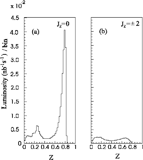
Figure 13.10: Luminosity distribution used in the Higgs analysis, where $z=\sqrt{s_{\gamma\gamma}}/2E_{beam}$. a) and b) are for the spin of two colliding photon system, $J_{z}=0$ and $J_{z}=\pm 2$, respectively.

Since the cross section of the Higgs boson and the background $q\bar{q}$ production depends strongly on the helicity combination as well as on the center-of-mass energy of the two-photon system, information about the differential luminosity,

$$\left.{{{dL}\over{d\sqrt{s_{\gamma\gamma}}}}}\right|_{J_{z}},$$

as shown in Fig. 13.10, is very important for a realistic simulation. In addition to the center-of-mass energy and spin combination of the colliding two photons, the rapidity of the system must be taken into account as well, since the energy of the colliding two photons is not always equal, while they are nearly equal for $e^{+}e^{-}$colliders. Figure 13.11 shows the center-of-mass energy versus rapidity of the two-photon system. In this figure, the rapidity ($\eta$) is defined as

$$\eta={1\over 2}ln{w_{1}\over w_{2}},$$

where $w_{1}$ and $w_{2}$ are the energy of the two photons. As expected from characteristics of the backward Compton scattering, the rapidity is smaller at a higher collision energy, and becomes larger in a lower energy region, meaning that the Higgs bosons are produced at rest, while background in lower energy region tends to escape into a small angle.

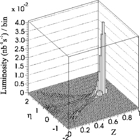
Figure 13.11: Rapidity versus the center-of-mass energy of two colliding photons.

The total $\gamma\gamma$ luminosity was calculated to be 3.4$\times 10^{32}\mbox{cm}^{-2}\mbox{s}^{-1}$ over the entire energy region.

For the intermediate-mass Higgs, the cross section of $\gamma\gamma\to H\to b\bar{b}$ near to the mass pole can be described by a Breit-Wigner approximation,

$$\sigma_{\gamma\gamma\to H\to b\bar{b}}=8\pi\frac{\Gamma(H\to\gamma\gamma)\Gamma(H\to b\bar{b})}{(s_{\gamma\gamma}-M^{2}_{H})^{2}+M^{2}_{H}\Gamma^{2}_{H}}(1+\lambda_{1}\lambda_{2}),$$ (13.7)

where $M_{H}$ is the Higgs-boson mass, $\Gamma(H\to\gamma\gamma)$, $\Gamma(H\to b\bar{b})$ and $\Gamma_{H}$ are two photons, $b$ quark pair and total decay width of the Higgs boson. $\lambda_{1}$ and $\lambda_{2}$ are the initial photon helicities.

For a realistic estimation of the Higgs production, the luminosity distribution calculated by CAIN was convoluted so as to estimate the number of generated events as

$$N=\sum\limits_{J_{z}}{\int{\sigma_{\gamma\gamma\to H}^{J_{z}}(s_{\gamma\gamma})}L_{J_{z}}(s_{\gamma\gamma})ds_{\gamma\gamma}},$$

where N and $s_{\gamma\gamma}$ are the number of events and center-of-mass energy of the $\gamma\gamma$  system. $J_{z}$ is the longitudinal component of the spin of the $\gamma\gamma$  system and the summation runs over the $J_{z}=0,2$ state. Throughout the analysis, we adopt quark masses of $m_{b}$=4.3 GeV, $m_{c}$=1.3 GeV, and $m_{t}$=176 GeV. The branching ratios ($Br(H\to b\bar{b})$, $Br(H\to c\bar{c})$, and $Br(H\to gg)$) are taken to be 64%, 2.7%, and 8.3%, respectively, which were calculated by the HDECAY program[35]. In HDECAY program, a $O(\alpha_{s}^{3})$ radiative correction by the $\overline{MS}$ scheme to the $\Gamma(H\to b\bar{b})$, was taken into account. The QCD correction affects the Higgs-boson production significantly and reduces the expected number of events by almost 50% of the tree level calculation around a Higgs-boson mass of 120 GeV.

Table 13.4: Effective cross sections and generated events with the luminosity distribution of the photon-photon collider.

	$\sigma_{|\cos\theta|<0.95}$ (pb)	Events	Simulated events
	(with Luminosity distribution)	(10 $\mbox{fb}^{-1}$)
Signal events
$\gamma\gamma\to H\to b\bar{b}$	0.508	5080	10000
Backgrounds ($\sqrt{s}>$ 75 GeV)
$\gamma\gamma\to H\to c\bar{c}$	0.0210	210	10000
$\gamma\gamma\to H\to gg$	0.0633	633	10000
$\gamma\gamma\to b\bar{b}(g)$	0.727	7270	10000
$\gamma\gamma\to c\bar{c}(g)$	15.1	151000	50000

A convolution with the luminosity distribution is performed by a Monte-Carlo integration package, BASES [36]. Kinematical cuts of $|\cos\theta|<0.95$ and $\sqrt{s}_{\gamma\gamma}>75$ GeV are imposed for effective event generation. The effective cross sections calculated with BASES are listed in table 13.4. The expected number of events of $b\bar{b}$ pairs from Higgs-boson decay is 5080 with an integrated luminosity of 10 $\mbox{fb}^{-1}$. For a further analysis, four-momenta of $b\bar{b}$ pairs from the Higgs boson decay are generated by the SPRING[36] program. Subsequent parton evolution and hadronization is simulated using the JETSET 7.3 [37] program with a parton shower and a string fragmentation prescription.

The $\gamma\gamma\to q\bar{q}$ background events are generated in a similar way as in Higgs production, except that the production amplitude is calculated by the helicity-amplitude calculation program HELAS[38], and that only events with $\sqrt{s_{\gamma\gamma}}>75$ GeV are generated. As mentioned in the previous section, QCD corrections have to be taken into account for a reliable background estimation. We use a calculation in [30] for this purpose, which includes the soft/hard gluon emission and virtual corrections. To simulate a $q\bar{q}g$ event, it is necessary to calculate the differential cross section of the process; however, it is reported in [30] that there is a difficulty to calculate the differential cross section with a small $y_{cut}$ value, where $y_{cut}$ is the minimum ’distance’ between two partons in terms of the invariant-mass squared to be regarded as two separated jets. The definition of the $y_{cut}$ is

$$y_{cut}\equiv{p_{i}p_{j}(1-cos\theta)\over s_{\gamma\gamma}},$$

where $p_{i}$, $p_{j}$ are the momentum of the $i$ and $j$th jet and $\theta$ is the angle between them. Thus we used the parton shower evolution in the JETSET program for event topology and scaled with the total cross section calculated in [30]. We discuss this point again in a later section.

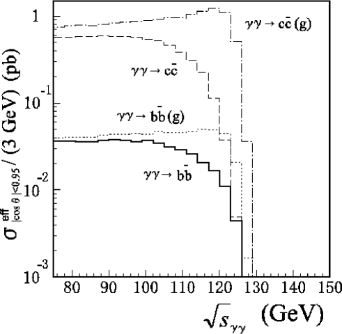
Figure 13.12: Effective cross sections with the luminosity distribution of the photon-photon collider at $P_{L}P_{e}=-1.0$. The solid line corresponds to $\gamma\gamma\to b\bar{b}$, the dashed line to $\gamma\gamma\to c\bar{c}$, the dotted line to $\gamma\gamma\to b\bar{b}$ with QCD corrections, and the dash-dotted line to $\gamma\gamma\to c\bar{c}$ with QCD corrections. The bin size is 3 GeV.

The effective cross sections and the number of generated events with the QCD corrections are listed in table 13.4. In this table, $\gamma\gamma\to q\bar{q}(g)$ indicates the process $\gamma\gamma\to q\bar{q}$, taking into account of the QCD corrections. Figure 13.12 shows the effective cross sections for the $J_{z}=0$ channel as a function of $\sqrt{s_{\gamma\gamma}}$. In this figure, in order to see the effect of the radiative correction, the effective cross sections with a tree-level calculation is shown as well. The suppression for $c\bar{c}$ and $b\bar{b}$ production works as the energy of $\gamma\gamma$  system increases, and even more for a lighter particle at the tree level. Once the suppression is removed by gluon emission, the effect is indeed very large. Thus, the effect of the radiative correction is large around $\sqrt{s}_{\gamma\gamma}$=120 GeV, and is much more significant for the $\gamma\gamma\to c\bar{c}$ process than for $\gamma\gamma\to b\bar{b}$.

In order to evaluate the performance of the Higgs-boson identification at a $\gamma\gamma$  collider, we performed a Monte-Carlo simulation using the JLC detector simulation program [39]. The main components used in the analysis are a vertex detector, a central drift chamber(CDC) and calorimeters. The $b$-quark tagging by the vertex detector(VTX) is crucial in this simulation. A CCD (charge coupled device) detector for the VTX is assumed in the current JLC-I design and its impact parameter resolution is

$$\sigma_{d}^{2}=11.4^{2}+(28.8/p)^{2}/\sin^{3}{\theta}\ (\mu\mbox{m}^{2}),$$ (13.8)

where $p$ is the momentum of the charged particle in GeV/c and $\theta$ is the angle with respect to the beam axis. The new parameter was used in the top found to be able to be improved The energy resolution of calorimeters, which plays the main role in the two-jet mass reconstruction, are $15\%/\sqrt{E}+1\%$ and $40\%/\sqrt{E}+2\%$ for electromagnetic and hadronic calorimeter, respectively.

The analysis requires a reconstruction of the two-jet final state from the Higgs-boson decay. In the analysis, the calorimeters are used for jet-mass reconstruction and the tracking detectors are used exclusively for b-quark tagging.

First of all, well reconstructed tracks and clusters in tracking devices and in calorimeters, respectively, are selected, and only these tracks and clusters are used in the analysis. A ‘good track’ requires $|\cos\theta|<0.95$, $P_{t}>0.1$ GeV/c; also the CDC track and VTX space points must be successfully linked. A ‘good cluster’ is defined as that of $E>0.1$ GeV and $|\cos\theta|<0.99$ among the clusters reconstructed in electromagnetic and hadron calorimeters.

The number of good tracks is required to be greater than 10 in order to choose multi-hadronic events. JADE clustering [40] is applied with $y_{cut}$=0.02 using good clusters to choose two-jet events. A cut of $|\cos\theta_{jet}|<0.7$ is applied, where $\theta_{jet}$ is the angle of the jet with respect to the beam axis, to ensure that the event is well contained in the fiducial volume.

To identify the $b\bar{b}$ final state, a $b$($\bar{b}$) jet is selected by requiring five or more tracks which have the normalized impact parameter $d/\sigma_{d}>2.5$ and $d<1.0\ \mbox{mm}$ in each jet, where $d$ is the impact parameter. Events of which both jets are identified as b-quark jets are regarded as being Higgs-boson candidates. With this requirement, the tagging efficiency of $b\bar{b}$ events is

$$\varepsilon_{tag}=\frac{\#\ \mbox{of tagged events}}{\#\ \mbox{of two-jet events}}.$$ (13.9)

Table 13.5 summarizes the tagging efficiencies and the number of events.

Table 13.5: Tagging efficiencies and the number of events with 10fb^-1.

	Tagging efficiencies (%)	Events
	$b\bar{b}$ tag	$b\bar{b}$ tag
Signal events
$H\to b\bar{b}$	59.5	582
Backgrounds
$H\to c\bar{c}$	19.7	7.85
$H\to gg$	6.17	1.58
$\gamma\gamma\to b\bar{b}(g)$	60.0	278
$\gamma\gamma\to c\bar{c}(g)$	14.9	1320

In order to enhance the signal, the mass region of the Higgs signal is chosen in such a way that the statistical significance of the signal, $(N_{obs}-\langle N_{bg}\rangle)/\sqrt{N}_{obs}$, is maximized, where $N_{obs}$ is assumed to be the number of observed events, while $\langle N_{bg}\rangle$ being the number of expected background events. As a result, events in two-jet mass regions of 106 GeV $<M_{jj}<$ 126 GeV are selected. The selection efficiency is defined as

$$\varepsilon_{sel}=\frac{\#\ \mbox{of selected events}}{\#\ \mbox{of generated events}}.$$ (13.10)

They are listed in table 13.6.

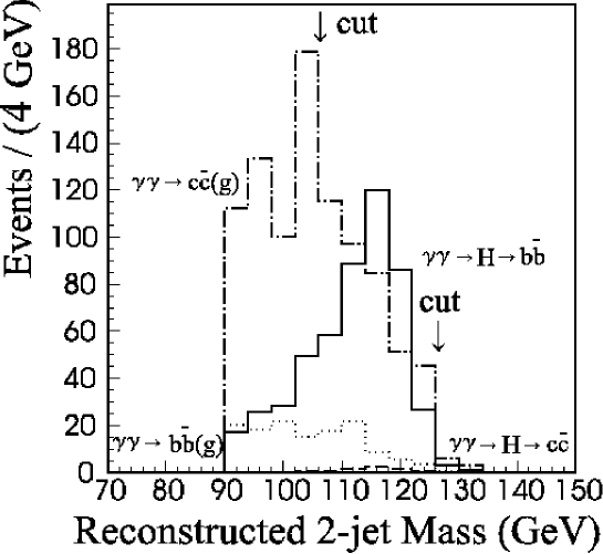
Figure 13.13: Mass distribution of two-jets with applying b-tagging requirements. An integrated luminosity of 10 $\mbox{fb}^{-1}$ and standard model branching fractions for the Higgs boson are assumed. The effects of the QCD corrections to $\gamma\gamma\to q\bar{q}$ as background process are included.

Table 13.6: Selection efficiencies and the number of events. The effects of the QCD corrections to $\gamma\gamma\to q\bar{q}$ as background process are included.

	$\varepsilon_{sel}$  (%)	Events
Signal events
$\gamma\gamma\to H\to b\bar{b}$	7.48	380
Backgrounds
$\gamma\gamma\to H\to c\bar{c}$	3.16	6.65
$\gamma\gamma\to H\to gg$	0.230	1.46
$\gamma\gamma\to b\bar{b}(g)$	0.790	57.4
$\gamma\gamma\to c\bar{c}(g)$	0.260	394
Signal to Background with QCD corrections		380 / 459

The statistical errors, $\sqrt{N}_{obs}/(N_{obs}-\langle N_{bg}\rangle)$, of the two-photon decay width of the SM Higgs boson at $M_{H}$=120 GeV is found to be 7.6%, assuming an integrated luminosity of 10${\rm fb}^{-1}$ with S/N=0.83. Any systematic error related to an estimation of background is not included in the result. As a reference, the statistical error with the tree-level calculation for $q\bar{q}$ was evaluated to be 6%.

Toward a further improvement of Higgs boson identification, it is crucial to reduce any contamination of c-quark jet within the b-quark jet candidates. Recently, a sophisticated method for b-quark identification was developed by the SLD group using the topological vertexing method [41]. It is reported that by using the topological vertexing method, the efficiency of b-quark jet identification and the purity are 70% and 0.7%, respectively, for equal mixing of c- and b-quark jets of 50 GeV within $|\cos\theta|<0.7$. Therefore, tagging efficiency of $b\bar{b}(g)$ and $c\bar{c}(g)$ events is 49% and 0.005% with double tagging, and 91% and 1.4% with single tagging method, respectively. Assuming that these numbers can be kept for Higgs-boson decay and $b\bar{b}/c\bar{c}$ production in the $\gamma\gamma$ collision, we can estimate the number of signal and the background.

For an estimation, we adapt the number of events surviving multi-hadron selection with $|\cos\theta_{jet}|<0.7$. The restriction for $|\cos\theta_{jet}|<0.7$ is applied to simulated events to fit the condition used in a topological vertexing analysis in [41]. The tagging efficiencies assumed in the estimation and the number of estimated events for signal and background are tabulated in table 13.7.

Table 13.7: Tagging efficiencies and the number of events by the topological vertexing method.

Tagging efficiencies	Double tag	Single tag
b jet	0.70	0.70
c jet	0.007	0.007
$H\to b\bar{b}$	0.49	0.91
$H\to c\bar{c}$	$5\times 10^{-5}$	0.014
$H\to gg$	0	0
$\gamma\gamma\to b\bar{b}(g)$	0.49	0.91
$\gamma\gamma\to c\bar{c}(g)$	$5\times 10^{-5}$	0.014
Number of expected events	Double tag	Single tag
within $106GeV<m_{jj}<126GeV$
$H\to b\bar{b}$	832	1545
$H\to c\bar{c}$	0	1.3
$H\to gg$	0	0
$\gamma\gamma\to b\bar{b}(g)$	121	223
$\gamma\gamma\to c\bar{c}(g)$	0.3	101
signal/background	832/121=6.9	1545/325=4.7
Statistical accuracy	3.7%	2.8 %

$\gamma\gamma\to c\bar{c}(g)$ contamination is now negligibly small, and only the $\gamma\gamma\to b\bar{b}(g)$ process is the major background. As a result, the statistical accuracy of the two-photon decay width is 3.7% and 2.8% by the double-tagging and single-tagging condition, respectively, which shows a good improvement from the conventional b-quark identification method. It is noted that the signal-to-background ratio(S/N) in this case is drastically improved as $S/N=812/121=6.9$ and $1545/325=4.7$ with the double and single tagging method, respectively, while it is 0.83 by the previous analysis. Since the background from $\gamma\gamma\to c\bar{c}$ is most serious and affected largely by an ambiguous radiative correction, an improvement of the signal-to-background ratio indicates a significant reduction of systematic errors coming from the background estimation.

This result shows that the $\gamma\gamma$  collider will be sufficient to distinguish the Higgs boson of MSSM from one of the standard model for an intermediate-mass Higgs boson when the ratio of the two-photon decay widths ($\Gamma(h^{0}\to\gamma\gamma,\mbox{MSSM})/\Gamma(H\to\gamma\gamma,\mbox{SM})$) is about 1.2 for a 120 GeV Higgs boson [22].

Recently, G. Jikia, M. Melles and their collaborators [42, 43] have performed aggressive studies on evaluating the effects of the radiative corrections with the resummation technique of double-logarithmic corrections, as well as the realistic Monte Carlo simulations with optimized event selection criteria. Applying some appropriate cuts, the statistical error of the measurement of the Higgs production cross section is estimated to be better than 2% for the Higgs mass between 100 and 140 GeV [43]. Such a high precision of this measurement can only be done at the photon-photon mode of the linear collider.

The heavy SM Higgs whose mass is heavier than the $W$-threshold mainly decays into a $W^{+}W^{-}$ pair. Since there is no tree diagram of the continuum background process, $\gamma\gamma\rightarrow ZZ$ mode is the promising channel to detect the heavy Higgs boson if its mass is heavier than $2m_{Z}$ [44, 45]. For the mass range between 140 GeV and 160 GeV, $\gamma\gamma\rightarrow WW^{*}$ mode is found to be available with some appropriate experimental cuts [46].

The detection methods for the SM Higgs boson is illustrated in the middle column of Table 13.8.

Table 13.8: The detection methods of Higgs bosons, which are strongly correlated with the dominant decay mode [47].

	SM	MSSM
light
$h^{0}$	$b\overline{b}$ mainly
heavy	$WW$ mainly	$WW$,$ZZ$ suppressed
$H^{0}$	$ZZ$ useful	$t\overline{t}$ mainly
	$t\overline{t}$ ?	$b\overline{b}$ for large $\tan\beta$
CP-odd		no $WW$,$ZZ$
$A^{0}$	—	$t\overline{t}$ mainly
		$b\overline{b}$ for large $\tan\beta$

More Complicated Higgs Models

If the Higgs sector has more complicated structure than that in the SM, one has to devise some other schemes to detect the various Higgs bosons. The minimal supersymmetric extension of the SM (MSSM) is one of the typical example of such new model which has a complicated Higgs sector.

In MSSM, there are three neutral Higgs bosons: the light CP-even Higgs $h$, the heavy CP-even Higgs $H$ and the CP-odd Higgs $A$. If we assume a large value of the $A$ mass, the light CP-even Higgs boson $h$ is similar to the light SM Higgs boson, and its detection can be done by the $b\overline{b}$ decay mode, just as the SM Higgs. However, for the heavy Higgs bosons, the situation is different. The $WW$ and $ZZ$ decay modes of $H$ are suppressed for heavy $A$ case, and these decays are forbidden for $A$ boson. Instead of them, $t\overline{t}$ decay mode may be useful, if the Higgs boson masses are heavier than $2m_{t}$, and if $\tan\beta\ll 10$. For the moderate and large values of $\tan\beta$, the decay mode to $b\overline{b}$ (and to $\tau^{+}\tau^{-}$ in some cases) is available [48]. The situation is also illustrated in Table 13.8. Furthermore, in the wide range of the MSSM Higgs parameter space, $H$ and $A$ often have similar values of mass. Then a question arises: Can we separate two signals of $A$ and $H$ at the photon-photon collider? Or, how do these signals of heavy Higgs bosons look like at a $\gamma\gamma$ collider?

The separation of $H$ and $A$ signals can clearly be done by using the linear polarization of the colliding photons. In the frame of the linear polarization of the initial photons, $H$ and $A$ states can only be produced from collisions of the parallel and the perpendicularly polarized photons, respectively [6, 7, 8, 9, 10]. That is the answer to separate the $H$ and $A$ signals.

$H$-$A$ interference in MSSM

With the circular polarization of the photon beams, there is another interesting story [49]. The circular polarization of the photon can be expressed in the 45-degree mixture of the two linear polarizations. It means that the collision of the circularly polarized photon beams is accessible to both the $H$ and $A$ amplitudes simultaneously. A similar situation can be seen in the decay of a Higgs state into a fermion pair in the definite helicity states, and the helicity of the top quark can be measured statistically by looking its decay angle distribution [51, 52, 53]. Then, the process of $\gamma\gamma\rightarrow t\overline{t}$ with circular photon polarization and top helicity detection has an interference effect of $H$ and $A$ amplitudes. The effect can be never observed if measuring of top quark helicity is not performed, because the interference term for $\gamma_{+}\gamma_{+}\rightarrow t_{R}\overline{t}_{R}$ cancels the one for $\gamma_{+}\gamma_{+}\rightarrow t_{L}\overline{t}_{L}$.

Table 13.9: Helicity dependence of the amplitudes for $\gamma\gamma\rightarrow H,A\rightarrow t\bar{t}$

	${\large t_{R}\bar{t}_{R}}$	${\large t_{L}\bar{t}_{L}}$
$\gamma_{+}\gamma_{+}$	${\cal M_{H}}$ ${\cal M_{A}}$	$-{\cal M_{H}}$ ${\cal M_{A}}$

In the process $\gamma\gamma\rightarrow t\overline{t}$, the above amplitudes interfere with the continuum amplitudes. By observing the interference effect, it is possible to judge whether a resonance is from $H$ or $A$. Denoting the helicity amplitudes for Higgs resonance $M_{\phi}^{LL{\rm or}RR}$ ($\phi=H$ or $A$) and of continuum process $M_{cont}^{LL{\rm or}RR}$, the helicity dependent interference terms are written by

$$sgn\left[{\cal M}_{\phi}^{RR}{\cal M}_{cont}^{RR}\right] = -sgn\left[{\cal M}_{\phi}^{LL}{\cal M}_{cont}^{LL}\right]\hskip 14.22636pt{\rm for}~{}~{}H,$$

$$sgn\left[{\cal M}_{\phi}^{RR}{\cal M}_{cont}^{RR}\right] = ~{}~{}~{}sgn\left[{\cal M}_{\phi}^{LL}{\cal M}_{cont}^{LL}\right]\hskip 14.22636pt{\rm for}~{}~{}A.$$ (13.11)

The difference appear in the cross section with circular polarized photons. Numerical results are shown in Fig. 13.14 (a,b). For definiteness, we use the MSSM prediction for the total and partial widths for $A$ adopted in ref. [49]. It is found that little interference is observed for $H$ (long-dashed curves) because the interference effects for $t_{L}\overline{t}_{L}$ and $t_{R}\overline{t}_{R}$ events cancel each other. On the other hand, the effects for $A$ (solid curves) can be large due to additive interference for both events.

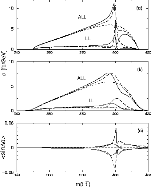
Figure 13.14: The $m(t\overline{t})$ dependence of the cross sections for $\gamma\gamma\rightarrow t\overline{t}$. The energy and polarization dependence of the $\gamma\gamma$ luminosity has been considered (we set the highest laser frequency, $x=4.83$ at $\sqrt{s}_{ee}=500$ GeV, and $P_{e}P_{L}=-1$.). Short-dashed curves show QED predictions, while solid (long-dashed) curves show predictions when $A$ ($H$) of $400$ GeV is produced. In (a) and (b), the thick lines are for total events and the thin lines are for events where final top-pairs are left-handed. Gaussian smearing with $\Delta m(t\overline{t})=3$ GeV is applied in (b). Azimuthal decay angular correlation is shown in (c) with (without) the smearing by thick (thin) lines.

G. Jikia and his collaborator calculated the QCD Next-to-Leading order correction to this process in an arbitrary photon beam polarization [54].

13.3.2 W Boson

Anomalous Coupling of the W bosons

The cross section of W pair production in the $\gamma\gamma$collision is about 90pb for $\sqrt{s_{\gamma\gamma}}>200$ GeV and is almost independent of the $\gamma\gamma$center-of-mass energy. This cross section is O($10-10^{2}$) higher than the fermion pair production, and is also O($10-10^{2}$) higher than the W pair production in $e^{+}e^{-}$collisions. It has been pointed out that the W pair production cross section in the $\gamma\gamma$interaction is sensitive to the anomalous coupling of W bosons to photons, $\delta\kappa_{\gamma}$[25, 55]. In this study, the feasibility of a measurement of the W pair production cross section in the $\gamma\gamma$collision and its sensitivity to the anomalous coupling of W bosons to photons have been investigated[56]. We studied a measurement of the W pair production cross section in a realistic condition, i.e., using a luminosity distribution simulated by CAIN, while taking the detector effect into account by simulation.

The laser and machine parameters used are almost identical to the 400GeV $\gamma\gamma$collider parameters listed in table 13.1. The difference is that the parameter used in this section assumes a relatively large CP-IP distance of 2cm and the spent electrons coming out from the CP are swept away from the IP by an external magnetic field. The $\gamma\gamma$luminosity was $6.9\times 10^{32}{\rm cm^{-2}s^{-1}}$ and $3.7\times 10^{32}{\rm cm^{-2}s^{-1}}$ in total and above the threshold of the W pair production, respectively. In a following study, the total integrated luminosity was assumed to be $10{\rm fb^{-1}}$, which corresponds to about one year of experimental operation.

The helicity amplitude for the $\gamma\gamma\to W^{+}W^{-}\to f\bar{f}f^{\prime}\bar{f^{\prime}}$ was calculated using the helicity amplitude calculation program HELAS[38]. The phase-space integration and event generation were performed by a Monte-Carlo integration (BASES) and event generation (SPRING) program[36], respectively. For a detector simulation, we adopted the JLC-I detector[39]; its performance, mainly related with this analysis, is the resolution of calorimeters, which are $15\%/\sqrt{E}+1\%$ and $40\%/\sqrt{E}+2\%$ for electromagnetic and hadronic calorimeter, respectively.

The W pair events were selected by 4-jet events, i.e., for the case that both the W bosons decayed into quark pairs. For each event, more than, or equal to, 10 charged tracks were required for the central tracking detector to be chosen as a multi-hadron event. After multi-hadronic event selection, JADE clustering[40] with $y_{cut}=0.007$ was applied and only 4-jet events were selected. 28% of the W pairs (60% of hadronic decay) survived the cuts. For remaining 4-jet events, $\chi_{W}^{2}$ was defined as

$$\chi_{W}^{2}\equiv{{\left({m_{ij}-m_{W}}\right)^{2}}\over{\sigma_{m}^{2}}}+{{\left({m_{kl}-m_{W}}\right)^{2}}\over{\sigma_{m}^{2}}},$$

where $m_{ij}$ is an invariant mass of the i-th and j-th jet combination and $m_{W}$ was the W mass. $\sigma_{m}$ is the resolution of the W-mass reconstruction, and was estimated to be 5 GeV by the simulation. One out of the possible three combinations which minimize $\chi_{W}^{2}$ was assigned to be the correct combination of jets from W decay. For the assigned jet combination, both W masses were required to be greater than 65 GeV and less than 95 GeV and $\left|{\cos\theta_{W}}\right|<0.9$, where $\theta_{W}$ is the angle of the W boson with respect to the beam axis. The overall detection efficiency by this selection was 15%.

The production cross section for W pairs weighted by luminosity,

$$\mathord{\buildrel\lower 3.0pt\hbox{$\scriptscriptstyle\frown$}\over{\sigma}}_{WW}\equiv\sum\limits_{J=1,2}{\int{{{dL_{\gamma\gamma}^{J}}\over{d\sqrt{s}}}\sigma_{WW}^{J}}}d\sqrt{s}$$

was approximately 50pb. Thus, the expected number of event with an integrated luminosity of 10${\rm fb}^{-1}$ is about 75000. In order to obtain the production cross section of W pairs, the center-of-mass energy of each event was calculated and put into 20 GeV bins. For each bin, the detection efficiency was estimated by a simulation to correct the cross section. Figure 13.15 shows corrected number of W pairs as a function of their center-of-mass energy.

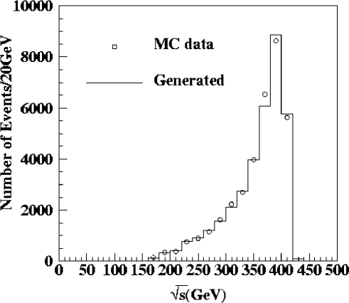
Figure 13.15: Number of W pair events as a function of the center-of-mass energy. The solid line is the number of generated and circles are the efficiency-corrected number of detected events. The normalization corresponds to a total integrated luminosity of 10${\rm fb^{-1}}$.

For the obtained number of events, the sensitivity to the anomalous coupling, $\delta\kappa_{\gamma}$ and $\lambda_{\gamma}$, were examined. Using the cross-section formula including the anomalous coupling parameter[25], the $\chi^{2}$ was defined as

$$\chi^{2}\equiv\sum\limits_{i}{\left({{{N^{i}-L_{0}^{i}\sigma_{0}^{i}-L_{2}^{i}\sigma_{2}^{i}}\over{\delta N^{i}}}}\right)^{2}},$$ (13.12)

where $N^{i}$, $L^{i}_{0}$, $\sigma^{i}_{0}$, $L^{i}_{2}$  $\sigma^{i}_{2}$ are the number of W pairs, the luminosity and the cross section for J=0 and 2 in the i-th bin, respectively. $\delta N^{i}$ is the error of $N^{i}$, and was estimated as

$$\delta N^{i}=\sqrt{N^{i}+\left({{dL_{0}^{i}}\sigma_{0}^{i}}\right)^{2}+\left({{dL_{2}^{i}}\sigma_{2}^{i}}\right)^{2}}.$$ (13.13)

The $dL_{k}^{i}$ in (13.13) is the error of the luminosity determination of the J=k component in the i-th bin, which will be described later. From the defined $\chi^{2}$ using (13.12), the expected 90% confidence limit in the $\delta\kappa_{\gamma}$-$\lambda_{\gamma}$ plain was calculated(Fig. 13.16).

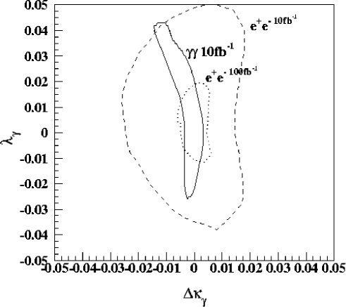
Figure 13.16: Expected 90% limit in W’s anomalous coupling parameter $\delta\kappa_{\gamma}$, $\lambda_{\gamma}$. An estimation with an $e^{+}e^{-}$collision is also shown by the dotted and dashed lines. The total integrated luminosity is assumed to be $10{\rm fb^{-1}}$.

As can be seen from the figure, the feasibility for a measurement of the anomalous coupling of W bosons by $\gamma\gamma$colliders is comparable to that from $e^{+}e^{-}$colliders. It should be pointed out that this feasibility is derived only from measurement of the total cross section, and improvements are expected by a comprehensive analysis using the decay property of W bosons.

Extra Dimensions

Arkani-Hamed, Dimopoulos and Dvali [57] have proposed that the existence of extra dimensions in which the gravity propagates can explain why the gravitational interaction is much weaker than the other elementary forces. The extra $n$ dimensions are compactified with some space scale and the corresponding mass scale is assumed to be a few TeV. In the scenario, the exchange of Kaluza-Klein graviton towers can contribute to various scattering processes at collider experiments. The Feynman rules have been developed by using the effective Lagrangian method. The graviton exchange could give rise to effective contact interactions between the SM particles in high energy scattering experiments [58]. In particular, the W-boson production at the $\gamma\gamma$ colliders could be affected sensitively by the graviton exchange contributions [59]. The precise measurement of the $W$-pair production cross section with appropriate initial beam polarization will give us the largest reach for the mass scale of the extra dimensions. The sensitivity on the scale of the cross sections is much better than those of other colliders as well as the other processes at $\gamma\gamma$ colliders such as the $\gamma\gamma$ and $ZZ$ productions [59, 60].

13.3.3 Top Quark

Physics with top quarks in the $e^{+}e^{-}$ linear collider has been studied and possibilities of rich physics with them has been demonstrated.(see chapter 4.) It has also been suggested that there are many topics of top quark physics to be explored in $\gamma\gamma$colliders. In particular, the $\gamma\gamma$collider has a unique feature that the polarization of initial state photons are controllable. The controllability of the polarization allows us to study aspects of physics which are virtually impossible with the $e^{+}e^{-}$colliders. However, there has been no realistic simulation analysis on the top quark pair detection in $\gamma\gamma$colliders so far. The estimation of detection efficiency and purity of the events is important since W boson pair production cross section is very large (about 90 pb independent of energy) and can be a serious background source.

In this study, we estimated the number of top quark events detected in a $\gamma\gamma$collider with a realistic luminosity distribution and with simulation for the JLC-I detector.

Production Cross Section

The effective top quark production cross section was calculated by convoluting luminosity distribution with the cross section as:

$$\hat{\sigma}_{t\bar{t}}\equiv{1\over{L_{tot}}}\sum\limits_{J=0,2}{\int{{{dL_{\gamma\gamma}^{J}}\over{d\sqrt{s_{\gamma\gamma}}}}}}\sigma_{t\bar{t}}\left({\sqrt{s_{\gamma\gamma}}}\right)d{\sqrt{s_{\gamma\gamma}}}$$ (13.14)

where the integration ran over the entire energy spectrum. The effective cross section defined in Eq. (13.14) was 0.17 pb which corresponds to the number of events as:

$$\halign{\hbox to\displaywidth{$\hfil\displaystyle#\hfil$}\cr 0.0pt{\hfil$\displaystyle N_{\exp}/year=\hat{\sigma}(\approx 0.17pb)\times L_{\gamma\gamma}/year(\approx 22.4fb^{-1})\cr 0.0pt{\hfil$\displaystyle\approx 4000\cr}}}$$

where a year of operation was assumed to be $10^{7}sec$.

The most serious background source for top quark events is W boson pair production. With the same definition as Eq.(13.14), production cross section of the W boson pairs is about 45 pb corresponding number of events in a year of 1.2 milion.[56] It is 300 times larger than that of top quark pair production. Suppression of this background is the most important issue for the analysis.

Event selection

The events were selected for two decay modes from top quark pairs.

• lepton + 4 jets; one top(anti-top) quark decays into a lepton, a neutrino and a b(anti b) quark jet, and the other goes to three jets.

• 6 jets; both top and anti-top quarks decay into three jets.

29% of top quark pairs decay into lepton + 4 jets while 46% decay into 6 jet mode. In both cases, final state jets include at least two b-quark jets. Thus, an efficient b-quark tagging is crucial to discriminate top quark events from W boson pairs.

The lepton + 4 jets events selection first required an isolated lepton in a hadronic event. The isolation required no particle within $20^{\circ}$ around the lepton. The JADE clustering algorithm [40] was applied for remaining events with varying $y_{cut}$ from 0.004 to 0.04 and the event had to have four hadronic jets at some $y_{cut}$. After selecting 4 jet events, b-quark jets were searched using the impact parameter method. The impact parameter resolution was assumed as:

$$\sigma_{b}(\mu m)=4.4+5.5/(p\sin\theta)^{2/3},$$

where p is the momentum of a track in GeV/c and $\theta$ is angle of the track with respect to the beam axis. In each jet, $N_{sig}$ was defined as the number of tracks having the impact parameter three times larger than $\sigma_{b}$. Then, two or more jets had to be $N_{sig}$ greater than one, and at least one jet had to be $N_{sig}$ greater than three. Finally, the jet-jet invariant masses were calculated for three possible combination and the one closest to the W boson mass was assigned to the W boson candidate. We required the jet-jet mass of the W boson candidate to be greater than 70 GeV. Fig. 13.17 shows jet-jet mass for the W boson candidate.

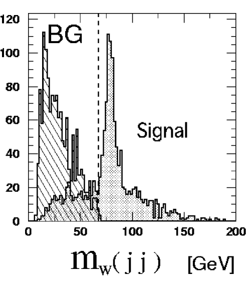
Figure 13.17: Jet-jet mass distribution for W boson candidate.

We obtained a detection efficiency of 9% with signal-to-background ratio of 10, corresponding to about 360 events per year.

For the 6 jet decay mode, an event must be classified as a 6 jet event by the same jet clustering algorithm as lepton + 4 jets analysis. For selected events, the b-quark tagging was applied in the same way as the lepton + 4 jet mode. 15.6% of top pair events survived the cuts with signal-to-background ratio of 10, which corresponds to 620 top quark events per year.

Toward Full Event Reconstruction

In order to apply selected top quark events to physics analysis, one has to reconstruct events and obtain, for example, angular distribution of top quarks. Here, we tried to reconstruct top quark angular distribution in the lepton + 4 jet mode.

To reconstruct top quarks from selected jets, we have to choose the right combination of W boson and b-quark jets. The W boson was already reconstructed in the event selection procedure. The remaining task is to choose the right b-quark jet out of two possibilities. In this analysis, both possibilities were tested and the combination where the reconstructed mass closer to the top quark mass was assumed to be the right one.

Fig. 13.18-a shows the angular distribution of reconstructed top quarks. It appears to reflect real angular distribution which is shown in Fig. 13.18, However, a more detailed study is necessary. Particularly, we still had order of 10% contamination from a wrong assignment of W boson and b-quark jet.

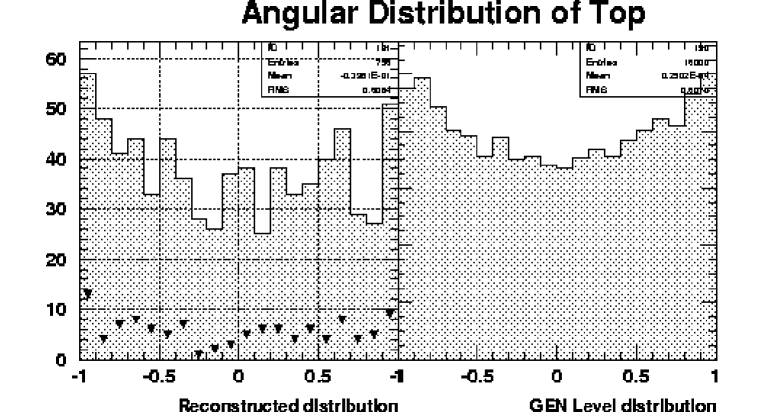
Figure 13.18: Angular distribution of the top quark at reconstructed (left) and at generated (right) level. Triangle points are contamination of miss-reconstructed events.

Summary on the SM top quark

We studied the feasibility of detection of top quark events in a $\gamma\gamma$collider as an option of the JLC. It was found we could detect about 1000 events with the signal-to-background ratio of 10 in a year of operation, i.e.,

• detection efficiency of 9% (360events/year) for lepton + 4 jets.

• detection efficiency of 15.6% (620events/year) for 6 jets.

A test of reconstruction of the angular distribution showed that it appeared to be possible to obtain information of the physical property of the top quark from the detected events. However more detailed simulation study is necessary to obtain quantitative estimation.

Top Quark Production in Technicolor Model

One of our most important tasks in the present particle physics is to understand the mechanism of electroweak symmetry breaking. Roughly speaking, the proposed models which go beyond the standard model are classified into two categories: supersymmetric models and composite models.

The composite models assume some new kinds of fermions which feel some additional strong interactions. A pair of new fermion and its anti-particle compose a vacuum condensate, which acts just like a Higgs field in the standard model. For example, in the technicolor model, new fermions which belong to SU(2)${}_{L}\times$U(1)_Y are assumed:

$$Q_{L}=\left({U\atop D}\right)_{L},\quad U_{R},\quad D_{R}.$$ (13.15)

To cancel the anomaly by themselves, the hypercharges of $Q_{L}$, $U_{R}$ and $D_{R}$ may be chosen as $0$, $1/2$ and $-1/2$, respectively. The above fermions also belong to the fundamental representation of the SU($N_{TC}$) gauge group of the new strong interaction, the so-called the technicolor, which is an analogue of QCD color. Due to technicolor, pairs of technifermion and anti-technifermion make some tight bound-states, just like mesons of quarks in QCD; however, the energy scale of the condensation is assumed to be at the weak scale. Among of the technimesons, technipions are consumed by $W$ and $Z$ bosons to acquire their masses.

If the energy of future colliders is high enough to create the technifermions or technimesons, of course we can examine new physics directly and in detail.

Since the top quark is known to have a heavy mass as the weak scale, it is natural in the technicolor model to expect that techniforce has some role to create the top-quark mass. It is often introduced as an effective four-fermion operator,

$$\frac{G}{M^{2}}\,({\bar{Q}}_{L}U_{R})({\bar{t}}_{R}q_{L})+{\rm h.c.},$$ (13.16)

where $G$ is the dimensionless coupling constant, $M$ the intrinsic mass scale of the operator, and $q_{L}$ the ordinary quark doublet of the top and bottom. The top-quark mass from the techniquark condensate can be estimated as

$$m_{t}=\frac{G}{M^{2}}\,\langle\bar{U_{L}}U_{R}\rangle.$$ (13.17)

The four-fermion interaction (13.16) can also affect the $\gamma\gamma\rightarrow t\bar{t}$ amplitude. The additional $\gamma\gamma\bar{t}t$ vertex function due to the techniforce can be parametrized by two form factors ($A$ and $B$) as

$$\Gamma^{\mu\nu}_{NEW}(k,\bar{k}) = Q_{U}^{2}\frac{G}{M^{2}}\{A(k,\bar{k})[(k\cdot\bar{k})g^{\mu\nu}-\bar{k}^{\mu}k^{\nu}]$$ (13.18)

$$\qquad\qquad+B(k,\bar{k})[k^{2}\bar{k}^{2}g^{\mu\nu}-k^{2}\bar{k}^{\mu}\bar{k}^{\nu}-\bar{k}^{2}k^{\mu}k^{\nu}+(k\cdot\bar{k})k^{\mu}\bar{k}^{\nu}]\},$$

where $Q_{U}$ is the electric charge of the techni-$U$ fermion, and the two photons have four-momenta $k$ and $\bar{k}$, and Lorentz indices $\mu$ and $\nu$, respectively [62]. Here the $B$ term vanishes after contacting the on-shell photon wave functions. The remaining $A$ form factor is assumed to have a pole-type function,

$$A(k,\bar{k})=\frac{r_{S}}{(k+\bar{k})^{2}-M_{S}^{2}},$$ (13.19)

to represent the contributing scalar channel [62]. Here, $M_{S}$ is the pole mass, which is taken to be the lowest-lying scalar technimeson mass. The value of $r_{S}$ can be estimated by computing $\Gamma^{\mu\nu}_{NEW}$ in Euclidean momentum space, and extrapolating it to the physical region with the ansatz (13.19).

The additional amplitude from $\Gamma^{\mu\nu}_{NEW}$ interferes destructively with the standard-model amplitude. Assuming the one-generation SU(3) technicolor model at the scale $M$ = 3 TeV, the cross section of the $\gamma\gamma\rightarrow t\bar{t}$ process for the same sign photon helicities is found to be suppressed for several percent at $\sqrt{s}_{\gamma\gamma}$ = 1 TeV [62]. The deviation from the standard model grows rapidly when the collider energy increases.

13.3.4 Supersymmetric Particle Productions

The supersymmetric (SUSY) standard model is the most promising extension of the standard model as it could naturally give a solution to the gauge hierarchy problem. The most phenomenologically important consequence of the model is in the fact that existence of the SUSY particles (sparticles) with masses $O$(100GeV$\sim$1TeV) are predicted. The search for these new particles and the study on their interactions must be an important purpose of the photon colliders as well as the LC and hadron colliders.

In estimation of the production rates for the sparticles at collider experiments, the automatic calculation codes could be very efficient since we must treat a large number of particles and unknown model parameters. GRACE[64] system is a code which generates automatically the matrix element in terms of helicity amplitudes for any process in the MSSM once the initial and the final states have been specified. We have developed an interface between GRACE and CAIN [5], which will be useful in extensive studies of the sparticle production at the photon colliders.

Chargino and Sfermion Production in $\gamma\gamma$ Collisions

In $\gamma\gamma$ collisions, the charged sparticles, the charginos ${\widetilde{\chi}_{i}^{\pm}}$ [1, 66, 67, 68, 69] and the sfermions ${\widetilde{f}^{\pm}}$ [1, 66, 67, 70], can be produced in pairs as far as it’s mass is below the kinematical bound,

$$\gamma\gamma \to {\widetilde{\chi}_{i}^{+}}{\widetilde{\chi}_{i}^{-}}$$ (13.20)

$$\gamma\gamma \to {\widetilde{f}}{\overline{\widetilde{f}}}$$ (13.21)

As they are pure SUSY QED processes, the cross sections to leading order depend only on the mass, the electric charge and the color degree of freedom of the sparticles. In other words, they do not have complicate dependence on the mixing angles of the sparticles as well as the weak gauge-boson contribution, which are inevitably involved in $e^{+}e^{-}$ collisions. This property could provide us complementary information about the models, e.g., universality of the masses for sleptons and squarks in the 1st and 2nd generations.

The mass dependence of the total cross sections with CAIN outputs for the photon spectrum is shown in Fig. 13.19, where we set $E_{e}$ $=$ 250GeV.

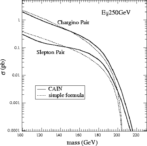
Figure 13.19: mass dependence of the total cross sections for chargino and slepton production. We take $E_{e}$ $=$ 250GeV. Solid and dashed line respectively corresponds to calculation with CAIN outputs and the simple formula for photon spectrum.

For a comparison, we also plot those with the simple photon spectrum formula [15, 16]. We find the cross sections become non-zero even above the naive kinematical bound,

$$m<0.8E_{e}.$$

In the calculation with GRACE and CAIN, the initial photon polarization has been appropriately included.

It should be emphasized that, as the $\gamma\gamma$ cross sections involve an $s$-wave contribution, they will be much larger than that of $e^{+}e^{-}$ if $\sqrt{s}$ is large compared to the mass threshold. This property not only provides large production rates compared to $e^{+}e^{-}$ collisions but also enables us to see the squarkonium production. We could detect a stoponium [71, 72] (sbottomonium) resonance peak in the invariant mass distribution for $\gamma\gamma\to\widetilde{t}_{1}\overline{\widetilde{t}}_{1}$ ($\gamma\gamma\to\widetilde{b}_{1}\overline{\widetilde{b}}_{1}$). From the peak structure, we could extract valuable information about the SUSY parameters as well as on the SUSY QCD.

Sfermion Production in $e\gamma$ Collisions

In $e\gamma$ collisions, a charged particle can be singly produced accompanied by a neutral one. Consequently, if there is large mass difference between the charged and the neutral particle, the kinematical limit for the production in $e\gamma$ collisions could be larger than that of pair production processes of each particle in $e^{+}e^{-}$ collisions.

In the framework of the MSSM we can assume ${\widetilde{Z}}_{1}$ as the LSP. In this case we find that the process

$$e\gamma\to\widetilde{e}_{R}{\widetilde{Z}}_{1}.$$ (13.22)

has a lower mass threshold of $m_{\widetilde{e}_{R}}+m_{{\widetilde{Z}}_{1}}$ than that of $2m_{\widetilde{e}_{R}}$ for the selectron pair production at $e^{+}e^{-}$ colliders. It is expected that $e\gamma$ colliders will be efficient in searching for the heavy selectron with a mass larger than half of $\sqrt{s}$ in $e^{+}e^{-}$ colliders [1, 73, 74, 75].

Figure 13.20 shows the selectron mass dependence of the total cross section.

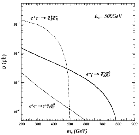
Figure 13.20: Selectron mass dependence of the total cross sections. We take $E_{e}$ $=$ 500GeV, $\tan\beta=12$, $\mu=-300{\rm GeV}$ and $M_{2}=200{\rm GeV}$, which correponds to $m_{{\widetilde{Z}}_{1}}=96{\rm GeV}$.

The selectron could be discovered up to the kinematical limit of $e\gamma$ collisions,

$$m_{\widetilde{e}}<1.8E_{e}-m_{{\widetilde{Z}}_{1}}.$$

We can obtain a large cross section for $e\gamma$ $\to$ $\widetilde{e}_{R}{\widetilde{Z}}_{1}$, even for the heavy selectron, $m_{\widetilde{e}_{R}}\mathrel{\vbox{\hbox{$>$}\nointerlineskip\hbox{$\sim$}}}E_{e}$. Note that the initial beam polarization will be efficient to enhance the signal cross section [1].

Another important property of the process is the simple dependence of the cross section on the SUSY parameters. The cross section is proportional to the bino component ($N_{11}$) of the lightest neutralino, ${\widetilde{Z}}_{1}=N_{11}\widetilde{B}+N_{12}{\widetilde{\rm W}}+N_{13}\widetilde{H}^{0}_{1}+N_{14}\widetilde{H}^{0}_{2}$. Arbitrary SUSY parameters appearing in the cross section are only $m_{\widetilde{e}_{R}}$, $m_{{\widetilde{Z}}_{1}}$ and $|N_{11}|$. This contrasts with the situation for the selectron pair production at $e^{+}e^{-}$ colliders, to which all masses and mixing angles of the neutralinos contribute. If we know $m_{\widetilde{e}_{R}}$ and $m_{{\widetilde{Z}}_{1}}$ from an analysis of the process $e^{+}e^{-}$ $to$ $\widetilde{e}_{R}^{+}\widetilde{e}_{R}^{-}$, we could determine $|N_{11}|$ by a measurement of the total cross section for $e\gamma$ $\to$ $\widetilde{e}_{R}{\widetilde{Z}}_{1}$.

In the framework of the MSSM with $R$-parity (lepton number) violating superpotential ($i\sim m$ denote generation indices) [76],

$$W_{/R}=\lambda_{ijk}L_{i}L_{j}{\overline{E}_{k}}+\lambda^{\prime}_{1lm}L_{1}Q_{l}{\overline{D}_{m}},\qquad\qquad(i\neq j\quad{\rm or}\quad k)=1$$ (13.23)

sleptons or squarks can be singly produced with ordinary matter fermions in $e\gamma$ collisions, e.g., through

$$e\gamma \to \ell_{i}\widetilde{\nu}_{j},\quad{\widetilde{\ell}}_{i}\nu_{j}\qquad\qquad(\lambda_{ij1}\neq 0),$$ (13.24)

$$e\gamma \to d_{m}\widetilde{u}_{l},\quad{\widetilde{d}}_{m}u_{l}\qquad\qquad(\lambda^{\prime}_{1lm}\neq 0).$$ (13.25)

In this case the kinematical limit becomes (except $e\gamma\to{\widetilde{d}}_{m}t$)

$$m\mathrel{\vbox{\hbox{$<$}\nointerlineskip\hbox{$\sim$}}}1.8E_{e}.$$

As an example we show the sneutrino mass $m_{\widetilde{\nu}_{\tau}}$ dependence of the total cross section for $e\gamma\to\mu\widetilde{\nu}_{\tau}$ in Figure 13.21.

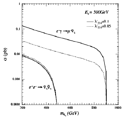
Figure 13.21: Sneutrino mass dependence of the total cross sections. We take $E_{e}$ $=$ 500GeV.

We find that the mass reach improves considerably in $e\gamma$ collisions in comparison with the pair ${\widetilde{\nu}_{\tau}}$ production at $e^{+}e^{-}$ colliders. Moreover, the SUSY parameter dependence of the cross section is simple in $e\gamma\to\mu\widetilde{\nu}_{\tau}$ becuase it is proportional to $|\lambda^{\prime}_{231}|^{2}$. It means that we can easily extract information on the ${/R}$ strength from the cross section measurements. On the other hand, it is not so easy in $e^{+}e^{-}\to\widetilde{\nu}_{\tau}{\overline{\widetilde{\nu}_{\tau}}}$, since the sensitivity on the coupling strength will be smeared owing to the $Z$-boson contribution, which does not depend on $\lambda^{\prime}_{231}$.

13.3.5 Excited Leptons in $e\gamma$ Collision

The $e\gamma$ collider is a suitable option for the search for excited electrons $e^{\ast}$[77, 78, 79]. If $m_{e^{\ast}}<\sqrt{s_{e\gamma}}$, a clear signal of $e^{\ast}$ as an $s$-channel resonance is expected. The production cross section is much larger than that of $e^{\ast}$ single production in $ee$ collision. The present lower limits of excited lepton masses are obtained as $\sim 90{\rm GeV}$ by LEP2 experiment [80, 81, 82]. $e\gamma$ colliders can extend the searchable mass range up to $\sqrt{s_{e\gamma}}$ ($\sim$ twice of $\sqrt{s_{ee}}$). Even if $m_{e^{\ast}}$ is beyond the energy range of the $e\gamma$ collider, its existence may be detectable by observing the interference with the standard model process.

By operating $e\gamma$ collider in such a mode to enhance the polarization of $\gamma$ and $e$ beams, we can get information on the coupling of $e^{\ast}$ to $e$ or more generally $e^{\ast}$ to leptons. Let us write the polarized cross section for the process $e\gamma\rightarrow e\gamma$

$$\begin{array}[]{rl}d\hat{\sigma}(\lambda,\xi_{2})=&\frac{1}{4}(1+\xi_{2})\{(1+2\lambda)d\hat{\sigma}[e_{R}\gamma_{+}]+(1-2\lambda)d\hat{\sigma}[e_{L}\gamma_{+}]\}\\ +&\frac{1}{4}(1-\xi_{2})\{(1+2\lambda)d\hat{\sigma}[e_{R}\gamma_{-}]+(1-2\lambda)d\hat{\sigma}[e_{L}\gamma_{-}]\},\end{array}$$

where $\lambda$ and $\xi_{2}$ are the mean helicity of electron and the Stokes parameter of $\gamma$, respectively. If $e^{\ast}_{L}$ couples radiatively to $e_{L}$ as suggested in some model [83, 84, 85], then the $s$-channel resonance is seen solely in the case $\lambda=-1/2,\xi_{2}=-1$. Conversely, if $e^{\ast}$ is observed as an $s$-channel resonance in $e_{R}\gamma_{+}$ mode, $e^{\ast}_{R}$ couples radiatively to $e$. Furthermore, if $e^{\ast}$ has spin 3/2, resonance in $e_{R}\gamma_{-},e_{L}\gamma_{+}$ mode are expected.

The value of $\xi_{2}$ cannot be tuned exactly but is determined by the polarization $P_{c}$ of initial laser beam and $\lambda^{\prime}$ of electron scattered by laser. For instance, by adjusting the polarization as $(P_{c},2\lambda^{\prime})=(1,-1)$, the energy of $\gamma$ beam concentrates on its kinematically allowed limit and $\xi_{2}$ is almost $-1$. Thus the $\gamma$ beam has a suitable polarization for the search for $e^{\ast}$ suggested by some model.

A sharp peak in the $z$ spectrum of the final states locates at $z_{\rm peak}=m_{e^{\ast}}^{2}/s_{ee}$ and $m_{e^{\ast}}$ is definitely determined. Background $\gamma$ due to QED process are produced in backward direction, an appropriate angular cut can make the signal clearer.

13.3.6 CP Violation Studies by Linearly Polarized Beams

One of the most important research subjects in the current particle physics is to explore the origin of the CP violation, which realizes the present universe filled with matter.

There are two techniques to observe the CP-odd quantities in high-energy collider experiments: one is to analyze the correlation of the spins and momenta of the final particles; the other one is to observe the angular distributions of the final particles, which are produced from the polarized initial beams. By tuning the polarizations of both the laser and the electron beam, one can obtain back scattered photon beam in almost arbitrary polarization demanded. Thus, a $\gamma\gamma$collider can be a unique probe to look for a different aspect of the CP violation through Higgs bosons, $t\bar{t}$ and $W^{+}W^{-}$ productions.

CP properties of Higgs bosons

As is already discussed in the section 13.3.1, the polarization of the photon beams is a very effective tool to analyze the CP properties of the Higgs bosons. One of such interest is on the $A$-$H$ intereference [49] which is already discussed in the above. Moreover, the method to determine the CP property of the heavy neutral Higgs bosons is recently discussed in the model without definite CP-parity [50]. It is a great advantage of the $\gamma\gamma$ collider that both of the circular and the linear polarizations of the photon beams can be available in high degree.

Top-Quark Electric-Dipole Moment(EDM) measurement

The top quark EDM bears an additional interaction between the top quark and the photon by a T-odd effective Lagrangian,

$${\cal L}_{EDM}=-ieQ_{t}\left(\frac{d_{t}}{2m_{t}}\right)\bar{t}\sigma_{\mu\nu}\gamma_{5}tF^{\mu\nu},$$ (13.26)

where $Q_{t}$ = 2/3, $m_{t}$ is the top-quark mass, $F^{\mu\nu}$ the photon field strength and $\tilde{\mu_{t}}$ $\equiv eQ_{t}d_{t}/2m_{t}$ the top-quark EDM. By observing the process $\gamma\gamma\rightarrow t\bar{t}$ with linearly polarized photon beams, one can extract the electric dipole moment (EDM) of the top quark. Detailed analyses can be found in [61, 86]. The CP-odd contribution to the differential cross section is proportional to

$$\eta_{1}\eta_{2}\,(1-\beta_{t}^{2}\cos^{2}\theta)\sin[2(\phi_{1}-\phi_{2})]\,{\rm Re}(d_{t}),$$ (13.27)

where $\eta_{1}$ and $\eta_{2}$ are the degrees of the linear polarization of the two photon beams, $\phi_{1}$ and $\phi_{2}$ are the azimuthal angles of the photon linear polarizations, and $\beta_{t}$ and $\theta$ are the velocity and the scattering angle of the top quark in the center-of-mass frame. It was found that only the number-counting method without the information of decaying top quarks is required here for the measurement of $d_{t}$. By adjusting the Compton-scattering conversion parameter ($x$), one can explore the top-quark EDM up to ${\rm Re}(\tilde{\mu}_{t})$ $=1.8$ and $0.2\times 10^{-17}$ $e\cdot{\rm cm}$ in the one-sigma level at $\sqrt{s}$ = 0.5 and 1.0 TeV machines with a 20 fb^-1 integrated luminosity, respectively [86]. This limit at 1.0 TeV is much smaller than that of $e^{+}e^{-}$ machines [87]. Poulose and Rindani also studied the dipole coupling using circularly polarized photon[88, 89]. A detail description is found in chapter 4.

W-boson Productions

The general form of the $\gamma WW$ vertex has seven independent terms, which characterize their Lorents structures [90]. Out of them, three terms violate CP symmetry. Due to the QED gauge invariance, one form factor of the three should vanish at $\gamma\gamma$ or $e\gamma$ collisions with the initial on-shell photons, and the remaining two, often called $f_{6}$ and $f_{7}$ in the literature, can be surveyed at the $\gamma\gamma$ and $e\gamma$ colliders. By adopting only the standard-model terms and the CP-odd terms, the effective $\gamma WW$ coupling would be expressed as

$$\Gamma^{\mu\nu\lambda}(q,\bar{q},k) = -ie\left[(q-\bar{q})^{\lambda}g^{\mu\nu}+(\bar{q}-k)^{\mu}g^{\nu\lambda}+(k-q)^{\nu}g^{\lambda\mu}\right.$$ (13.28)

$$\qquad\left.+f_{6}\epsilon^{\mu\nu\lambda\rho}k_{\rho}+\frac{f_{7}}{m_{W}^{2}}(q-\bar{q})^{\lambda}\epsilon^{\mu\nu\rho\sigma}k_{\rho}(q-\bar{q})_{\sigma}\right],$$

where $q$, $\bar{q}$ and $k$ are the $W^{-}$, $W^{+}$ and $\gamma$ momenta, and $\mu$, $\nu$ and $\lambda$ are the Lorentz indices of their external bosons, respectively.

The $f_{6}$ depencence of the differential cross section in the process $\gamma\gamma\rightarrow W^{+}W^{-}$ vanishes in the leading order of $f_{6}$, when the directions of the linear polarizations of the colliding two photon beams are parallel. However, it maximizes and is proportional to ${\rm Re}(f_{6})\,\sin 2\phi$ when the two beam polarizations are perpendicular, where $\phi$ stands for the azimuthal angle of the scattered $W$ boson with respect to the direction of the linear polarization of one beam [25].

With an integrated luminosity of 20 fb^-1 at $\sqrt{s}$ = 500 GeV, a $\gamma\gamma$ collider can measure the ${\rm Re}(f_{6})$ up to an accuracy of $2.3\times 10^{-2}$ and up to $0.6\times 10^{-2}$ with 100 fb^-1 at 1 TeV [25]. These bounds are given at the $3\sigma$ level.

The imaginary part of $f_{6}$ is accessible up to $1.2\times 10^{-3}$ at 0.5 TeV with 20 fb^-1 by using the circular photon polarization [25].

The process $e^{-}\gamma\rightarrow\nu W^{-}$ is also effective to measure the CP-odd form factor $f_{6}$, only if the helicity of the final $W^{-}$ is understood [25].

13.3.7 Hadronic Cross-sections in $\gamma\gamma$ collisions

An accurate knowledge of hadronic cross-sections in $\gamma\gamma$collisions ($\sigma_{\gamma\gamma}^{\rm had}$) at high energies is of two fold importance. It is very interesting from a theoretical view point of acquiring an almost ‘first principle’ understanding of a nonperturbative quantity such as total/inelastic cross-sections in a QCD based picture. On a more pragmatic note it is essential to be able to estimate the hadronic backgrounds at the future Linear colliders, both in the $e^{+}e^{-}$  and the $\gamma\gamma$  mode. It should be pointed out right at the beginning that even though the quantity $\sigma_{\gamma\gamma}^{\rm had}$ can be measured at an $e^{+}e^{-}$  collider as well, the Compton colliders will play a very important role in realizing the first of the above stated aims, due to the ’unfolding’ procedures that have to be used to extract the $\gamma\gamma$  cross-section from the measured hadronic cross-sections for the process $e^{+}e^{-}\to e^{+}e^{-}\gamma\gamma\to e^{+}e^{-}+$ hadrons.

Different theoretical models for the hadronic $\gamma\gamma$  cross-sections and discrimination among them at the $\gamma\gamma$  colliders

It is now well established that all the hadronic cross-sections $pp/p\bar{p}$, $\gamma p~{}$ and $\gamma\gamma$  rise with the energy of the colliding beams. The latter two, involving the hadronic structure of the photon, have become available only recently from HERA [91, 92] and LEP [93, 94]. A variety of models [95], some using factorization along with a generalization of the phenomenological ideas introduced to describe the rise with energy observed for the $pp/p\bar{p}$ cross-sections [96], treating the photon like a proton and some based on QCD, using the information on the parton structure of the photon, have been put forward. In all these descriptions, the extra parameters required for the case of the photon are mostly determined from the $\gamma p$ case and then cross-sections are predicted for the $\gamma\gamma$  case. Present $\gamma p$ and $\gamma\gamma$  data seem to indicate that the energy rise of the cross-sections involving photons might be faster than that for the $pp/p\bar{p}$ case, which is expected generally in the ‘eikonalised minijet’ models [97, 98]. However, the values of $\sigma_{\gamma p}^{\rm had}$, $\sigma_{\gamma\gamma}^{\rm had}$ at HERA and LEP respectively are extracted from a study of the reactions $ep\to e\gamma p\to eX$ and $e^{+}e^{-}\to e^{+}e^{-}\gamma\gamma\to e^{+}e^{-}X$, respectively. As a result the errors in the extracted experimental values are substantial. Within those errors, predictions of some of these other models also tend to be consistent with the data. Thus a $\gamma\gamma$  collider which does not suffer from the ‘unfolding’ problems can serve very well indeed for discriminating between these various theoretical models and achieving a better understanding of the theoretical situation.

The left panel of Fig. 13.22

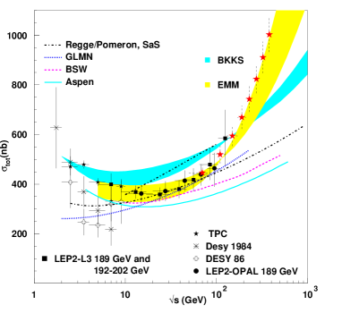
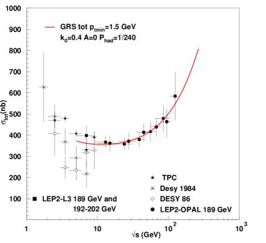
Figure 13.22: The predictions from factorization models, Regge-Pomeron exchange and a QCD structure function models together with those from the EMM and a comparison with present data in the left panel and the EMM description of the latest LEP data for parameters extracted from $\gamma p$ with $10\%$ changes [98] in the right panel as an illustration.

shows a compilation of the latest data on the $\gamma\gamma$ cross-sections and the predictions of the different models. A parameterization of the various model predictions in the form

$$\sigma_{\gamma\gamma}^{~{}\rm had}(s_{\gamma\gamma})=a~{}s_{\gamma\gamma}^{\epsilon}+b~{}s_{\gamma\gamma}^{-\eta}.$$ (13.29)

gives $\epsilon$ values between 0.09 (Aspen model)[99], 0.13 (BKKS) [100] and 0.30(Eikonalised minijet models EMM)[98, 97]. The QCD based models [98, 100] seem to describe the current data somewhat better. The figure shows also the expected $\gamma\gamma$  cross-sections at a Compton collider for a 500 GeV Linear Collider with TESLA design, in the ‘minijet’ models, for a choice of parameters which produces the ‘best fit’ to the LEP data and is consistent with the $\gamma p$ HERA data [98, 101], as ‘pseudo data points’ expected to be measured at such a collider. These are indicated by the red stars, with estimated errors [102] on them indicated by the vertical bars. In the right panel of the same figure the EMM prediction in its total formulation is shown along with the latest L3 data. The values of the parameters of the EMM used here are consistent with the $\gamma p$ data within $10\%$ uncertainty.

The difference in the rate of the rise with energy of the predicted $\gamma\gamma$ cross-sections, is seen more clearly in Fig. 13.23

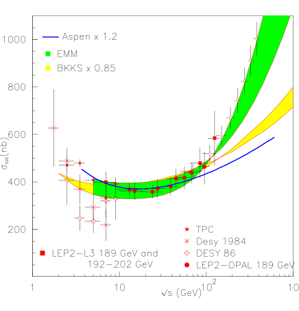
Figure 13.23: The total $\gamma\gamma$  cross-section as a function of the collision energy compared with some model calculations: BKKS band [100] band corresponds to different partonic densities for the photon, EMM band corresponds to the different choices of parameters in the EMM model [97, 98], the solid line corresponds to a proton like model [99]. The Aspen and BKKS results have been normalized to the data.

where the predictions of the Aspen and BKKS model have been normalized to the data. This figure again has the same ‘pseudo data points’ as shown in the Fig. 13.22. This figure shows very clearly that $\gamma\gamma$  collider will be able to indeed discriminate between these models and clarify our theoretical ideas about the high energy behavior of the total hadronic cross-sections.

In Table 13.10 we show the expected total $\gamma\gamma$ cross-sections for three different models which treat a photon more or less like a proton  [99, 103, 104]. The last column shows the 1$\sigma$ level precision needed to discriminate between Aspen[99] and BSW[103] models. The difference between DL[104] and either Aspen or BSW is bigger than between Aspen and BSW at each energy value.

Table 13.10: Precision required for the measurement of $\gamma\gamma$  cross-sections to distinguish between the different ‘proton’ like models

$\sqrt{s_{\gamma\gamma}}(GeV)$	Aspen	BSW	DL	$1\sigma$
20	309 nb	330 nb	379 nb	7%
50	330 nb	368 nb	430 nb	11%
100	362 nb	401 nb	477 nb	10%
200	404 nb	441 nb	531 nb	9%
500	474 nb	515 nb	612 nb	8%
700	503 nb	543 nb	645 nb	8%

A similar table can be drawn for distinguishing between the total and inelastic formulation of the minijet models [98] and the BKKS model[100], for instance.

Table 13.11: Precision required for the measurement of $\gamma\gamma$  cross-sections to distinguish between different formulations of the EMM and BKKS [100]

$\sqrt{s_{\gamma\gamma}}(GeV)$	EMM, Inel,GRS	EMM, Tot,GRV	BKKS	$1\sigma$
	($p_{\rm tmin}$=1.5 GeV)	($p_{\rm tmin}$=2 GeV)	GRV
20	399 nb	331 nb	408 nb	2 %
50	429 nb	374 nb	471 nb	9%
100	486 nb	472 nb	543 nb	11%
200	596 nb	676 nb	635 nb	6%
500	850 nb	1165 nb	792 nb	7 %
700	978 nb	1407 nb	860 nb	13 %

The last column in Table 13.11 now gives the percentage difference between the two models which bear closest results, i.e. EMM with GRS [105] densities and inelastic formulation on the one hand and BKKS, as well as EMM with GRV [106]densities and total formulation on the other. From the two tables one sees that a measurement to $7\%$ accuracy, will be able to distinguish within a class of models of a particular type. Figs. 13.22,13.23 shows that for a distinction between the different classes even a precision of $\>\raisebox{-2.15277pt}{$\stackrel{{\scriptstyle\textstyle<}}{{\sim}}$}\>20\%$ is sufficient, for the $\gamma\gamma$  energies of up to $\sqrt{s}<500$ GeV.

Hadronic backgrounds at the future colliders

One of the ways of estimating the hadronic backgrounds will be indeed to use the measured values of the hadronic $\gamma\gamma$  cross-sections from LEP in a parameterized form. Due to the somewhat larger errors in the highest energy data points as well as the uncertainties caused by having to extrapolate the measured two photon hadronic cross-section outside the kinematic region covered by measurements, the current data are consistent with pretty different behavior of the values of positive exponent of $\sqrt{s_{\gamma\gamma}}$ in the parameterization of the data. In Table 13.12 we give the fitted values for the parameters $\epsilon,\eta$ of Eq. 13.29, for different model predictions. Note here that this is just a parameterization of the curves drawn in the left panel of Fig. 13.22. Only representative values of the parameters in each case have been given. A more complete job by giving the dependence of these powers on the parameters of the model, e.g. the minimum $p_{t}$ used $p_{t}^{min}$ or $k_{0}$ the parameter determining the overlap function in the case of the ‘minijet’ models, would indeed be welcome. In the table numerical values obtained from the fit to the lower most and upper most curves of the EMM and BKKS bands as well as those for Aspen model are given.

Table 13.12: Values of the parameters a,b,$\eta,\epsilon$ of Eq. 13.29 obtained by numerical fits to the various model predictions.

Model	a(nb)	$\epsilon$	b(nb)	$\eta$
BKKS (upper edge)	166.5	0.13	538.2	0.38
BKKS (lower edge)	180.6	0.11	356.5	0.18
Aspen	145.7	0.094	517.5	0.39
EMM (lower edge)	14.01	0.34	475.4	0.14
EMM (upper edge)	19.9	0.29	475.3	0.084

Note here that this parametrization should be used only for $\sqrt{s_{\gamma\gamma}}>10$ GeV or so. It should be mentioned here that the ‘minijet’ models in their current formulation do have certain lacuna when confronted with the $pp,p\bar{p}$ along with the $\gamma p$ , $\gamma\gamma$  data [109, 110]. This indicates the need to modify the modeling of the overlap function which is not strictly calculable from first principles. A QCD model for this has been proposed [109]. Work is in progress to apply the Bloch-Nordsieck approach to photon-induced processes. This is expected to tamper the high energy rise somewhat. What would be even more interesting is to study the implications of the Bloch-Nordsieck formalism to multiplicity distributions or for multiple parton processes to determine the parameters of the EMM model using these. The values given in Table 13.12 represent the spread of our predictions at present.

Yet another ’rule of thumb’ measure of the ‘messiness’ at the Compton colliders can also be obtained by looking at the quantity $\sigma^{\rm jet}_{\gamma\gamma}$ defined

$$\sigma^{\rm jet}(s,p_{\rm tmin})=\int_{p_{\rm tmin}}d^{2}{\vec{p}_{t}}{{d\sigma_{jet}}\over{d^{2}{\vec{p}_{t}}}}.$$ (13.30)

where the $d\sigma_{jet}/d^{2}{\vec{p}_{t}}$ is calculated using perturbative QCD and photonic parton densities measured experimentally. This rises steeply with increasing energy and decreasing $p_{\rm tmin}$. While it is true that only part of this rise with $\sqrt{s}$ is reflected in the energy dependence of $\sigma^{\rm had}$, the quantity is still a good measure of the messiness caused by the hadronic backgrounds at the JLC due to beamstrahlung. Here we give a new parameterization of the ‘minijet’ cross-sections in $\gamma\gamma$  collisions which can be used in estimating the hadronic backgrounds at the JLC’s by folding it with appropriate beamstrahlung spectra. This supersedes the corresponding parameterization that was given earlier [107].

The ’minijet’ cross-section, for the GRV [106] and SAS [108] densities, is given (in nb)

$$\sigma_{minijet} = \left[222\left({2\;{\rm GeV}\over p_{\rm tmin}}\right)^{2}-161\left({2\;{\rm GeV}\over p_{\rm tmin}}\right)+36.6\right]\left({\sqrt{s}\over 50}\right)^{1.23}$$ (13.31)

$$= \left[77.6\left({2\;{\rm GeV}\over p_{\rm tmin}}\right)^{2}-45.9\left({2\;{\rm GeV}\over p_{\rm tmin}}\right)+9.5\right]\left({\sqrt{s}\over 50}\right)^{1.17}$$ (13.32)

by Eqs. 13.31 and 13.32 respectively. Here $\sqrt{s}$ is the $\gamma\gamma$  c.m. energy in GeV.

It is essential to fix $pt_{\rm tmin}$ due to the very strong dependence of the $\gamma\gamma$  ‘minijet’ cross-section on it. From our earlier discussions it is clear that this value will be $\sim 2$ GeV.

Is discrimination still possible with only an $e^{+}e^{-}$collider?

While it will be difficult to measure the $\sigma^{\rm had}_{\gamma\gamma}$ in the $e^{+}e^{-}$  mode with sufficient accuracy some information can still be gained by measuring $\sigma(e^{+}e^{-}\to e^{+}e^{-}~{}{\rm hadrons})$. This can be calculated by convoluting the $\gamma\gamma$  hadronic cross-sections with the spectrum of the photons. This spectrum is given by the Weizäcker Williams approximation for the bremsstrahlung photons. The approximation has to be improved to include the effect of the virtually of the photons. The expected hadronic cross-section due to the two photon processes at an $e^{+}e^{-}$  collider is shown in Fig. 13.24.

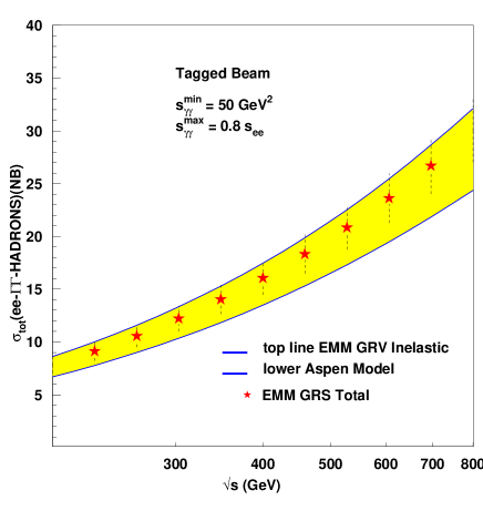
Figure 13.24: Cross-sections for hadron production due to $\gamma\gamma$  interactions in $e^{+}e^{-}$reactions. The red stars indicate the expected cross-sections in the EMM model, in total formulation with GRS densities with error bars representing the estimated errors.

The integration over $s_{\gamma\gamma}$ is restricted to a minimum value such that corrections due to losses along the beam direction can be made with precision and errors due to the unfolding are reduced. An upper limit is imposed to reduce the contamination by the annihilation events. The figure corresponds to a choice of $50\ GeV^{2}<s_{\gamma\gamma}<0.64s_{ee}$. The top curve here corresponds to the inelastic formulation of the EMM model [98] with GRV densities and the lower curve to Aspen model [99]. The ’pseudo data points’ expected for the total formulation of the EMM with GRS densities with the choice of the parameters used in the figure in the right panel of Fig. 13.22. The vertical error bars are the errors expected at TESLA [102]. The figure thus clearly shows that even a $e^{+}e^{-}$  collider will be able to shed some light on the issue of hadronic $\gamma\gamma$  cross-sections.

Summary

Thus in conclusion we can say the following

1. ’Photon is like a proton’ models predict a rise of $\sigma_{\gamma\gamma}$ with $\sqrt{s_{\gamma\gamma}}$, slower than shown by the data, albeit compatible with them within 2 $\sigma$, i.e. value of predicted $\epsilon$ is lower than what the data seem to show.

2. The extrapolated $\gamma p$ data seem to show similar trends.

3. The predictions of the EMM model show good agreement with the data.

4. Even in the EMM formulations use of Bloch Nordsieck ideas to calculate the overlap function $A(b)$ seems to slow down this rise.

5. An obvious improvement in the EMM models is to try and determine $A(b)$ by more refined ‘theoretical’ ideas or determine it in terms of the multiple parton interactions measured at the HERA/Tevatron collider.

6. However, extraction of $\sigma_{\gamma\gamma}$ and $\sigma_{\gamma p}$ from $\sigma_{e^{+}e^{-}}$ and $\sigma_{ep}$ respectively, is no mean task and has large uncertainties. Moreover, a difference of about a factor two in the predicted values of $\sigma^{\rm tot}_{\gamma\gamma}$ in different models, gets reduced to only about $30\%$ when folded with the photon spectrum expected in the WW approximation in $e^{+}e^{-}$ collisions. While the good part is that it reduces the uncertainty in our predictions of the hadronic background at the $e^{+}e^{-}$ linear colliders due to the corresponding uncertainties in $\sigma^{\rm tot}_{\gamma\gamma}$, the studies of two-photon hadronic cross-sections at $e^{+}e^{-}$ colliders, will not be very efficient in shedding much light on the theoretical models used to calculate them.

7. Therefore measurements of total cross-sections at a $\gamma\gamma$ collider with its monochromatic photon beam, in the energy range $300<\sqrt{s_{\gamma\gamma}}<500$ GeV, can play a very useful role in furthering our understanding of the ’high’ energy photon interactions. A precision of $\>\raisebox{-2.15277pt}{$\stackrel{{\scriptstyle\textstyle<}}{{\sim}}$}\>7-8\%(8-9\%)$ is required to distinguish among the different formulations of the EMM models (models which treat photon like a proton), whereas a precision of $\>\raisebox{-2.15277pt}{$\stackrel{{\scriptstyle\textstyle<}}{{\sim}}$}\>20\%$ is required to distinguish between these two types of models.

13.3.8 Luminosity Measurement

At the $e^{+}e^{-}$collider, Bhabha scattering has large cross section and is a good channel to monitor the luminosity[111, 112]. In the $\gamma\gamma$ collider, there is no such processes having a large cross section as Bhabha scatting in the $e^{+}e^{-}$ interaction. In addition, the luminosity spectrum of the $\gamma\gamma$ collision is far from the monochromatic and, information of the polarization is essential for physics study. Therefore, to pursue good physics at the $\gamma\gamma$  collider, measurement of differential luminosity as:

$${{dL}\over{dE_{\gamma}^{1}dE_{\gamma}^{2}d\xi_{\gamma}^{1}d\xi_{\gamma}^{2}}}$$ (13.33)

where $E_{\gamma}^{1(2)}$ and $\xi_{\gamma}^{1(2)}$ are the energy and polarization of the first(second) photon. It can be equivalently expressed in away which is more suitable for physics analysis as

$${{dL^{J=0,2}}\over{d\sqrt{s_{\gamma\gamma}}d\eta_{\gamma\gamma}}}$$ (13.34)

for helicity based analysis or

$${{dL^{\parallel,\bot}}\over{d\sqrt{s_{\gamma\gamma}}d\eta_{\gamma\gamma}}}$$ (13.35)

Here, $\eta_{\gamma\gamma}$ is the rapidity of the $\gamma\gamma$  system defined as

$$\eta_{\gamma\gamma}=\log\sqrt{E_{1}/E_{2}},$$

, $J$ is (z component of) total spin of the photon photon system and $\parallel$($\bot$) stands for that the electric field of two photons are in parallel(perpendicular) each other.

For a good measurement of the luminosity, processes must have large cross sections and can be selected with high efficiency with small background contamination. The possible candidate processes are; $\gamma\gamma\rightarrow e^{+}e^{-}$, $\gamma\gamma\rightarrow\mu^{+}\mu^{-}$, $\gamma\gamma\to W^{+}W^{-}$. The lepton pair production are good processes, however, it is only sensitive to the J=2 component of the luminosity so that it is necessary to measure total luminosity by other processes. The total cross section of $\gamma\gamma\rightarrow\mu^{+}\mu^{-}\mu^{+}\mu^{-}$, is as large as about 150pb independent of energy, however, most of muons are radiated in to the beam direction. For, example, if we require that at least two like sign muons are $\left|{\cos\theta<0.98}\right|$ and $E>1GeV$, the effective cross section goes down to about 2pb at 100GeV and 0.1pb at 400 GeV. The radiative electron positron pairs, i.e., $e^{+}e^{-}\to e^{+}e^{-}\gamma$ could be useful for the luminosity measurement[65]. Though the cross section does not appear to be large enough for high energy but could be till useful for luminosity measurement below W boson threshold. If we assume that W is the standard model gauge boson, the W pair production is a good candidate for a luminosity measurement at a center-of-mass energy greater than 200 GeV.

A possibility of measuring polarization dependent luminosity using lepton pairs were proposed[113]. When the $\gamma\gamma$ collider is running with $P_{L}P_{e}=-1$, the helicities of two photon beams are usually chosen to have the luminosity distribution of either the J=0 or J=2 dominant distribution. These two modes can be easily exchanged if both $P_{L}$ and $P_{e}$ are flipped simultaneously for one of the photon beams. This operation keeps $P_{L}P_{e}=-1$ but changes the sign of the helicity of the generated photons, making it possible to exchange between J=0 and J=2 mode without, in ideal condition, changing luminosity distributions. Thus, with this helicity-flipping method, the J=0 luminosity can be directly given by the measured J=2 luminosity.

A feasibility study for a luminosity measurement was performed for the process $\gamma\gamma\rightarrow e^{+}e^{-}$ and for $\gamma\gamma\rightarrow W^{+}W^{-}$ [56, 1]. The reconstructed luminosity distribution and the statistical errors on the luminosity measurements are shown in Fig. 13.25.

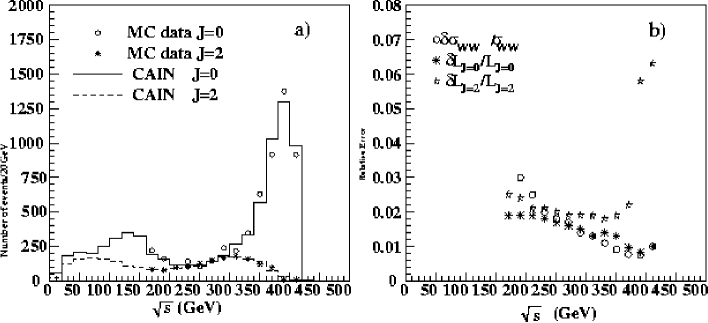
Figure 13.25: a) Reconstructed events at the process $\gamma\gamma\rightarrow e^{+}e^{-}$,where the circles and asterisks are the measured luminosities with J=0 and J=2, while the solid and dashed lines are the generated luminosities with J=0 and J=2, respectively. b) Estimated statistical error for the luminosity measurement, assuming the integrated luminosity of $10fb^{-1}$.

As shown in this figure, for both electron and W pairs, the statistical errors are expected to be $1\sim 2$% for each energy bin. This measurement assumes, however, the use of sophisticated helicity flipping to obtain polarized luminosities which potentially has systematic effects. More detail study on the systematic effect of the measurement is necessary on this point.

13.4 Technical Issues

In a current design of the $\gamma\gamma$  and $e\gamma$  collider, all particles from the conversion point are brought to the interaction region and experience the beam beam interaction. In addition, the $\gamma\gamma$  and the $e\gamma$ collider needs TW laser pulses synchronized with the electron beam at the conversion point which is about a half $cm$ from the interaction point. It adds technical issues to be solved in addition to the $e^{+}e^{-}$  collider, i.e.,

• Development of high-repetition/high-power lasers.

• Optical system for laser pulses in the interaction region.

In following sections, the status of the design of the interaction region and the laser system will be described.

13.4.1 Interaction Region

The issue on the interaction region are:

• Protect detectors from the beam-beam backgrounds.

• Extract spent electron beam.

• Take TW laser pulses in and out from the interaction region without hitting anywhere.

In the sense of the beam related background, situation is more or less similar to the $e^{+}e^{-}$  collider except energy spectrum of the spent electron. Since the electron beam already interacted with the laser pulse at the conversion point, energy of the electron beam is widely spread and the energy could be as low as O(GeV) which are disrupted away to the detector volume.

To estimate the beam-beam effect, CAIN was employed to simulate the interaction of electron bunches when they are passing by. Figure 13.26 shows a plot of disrupted electrons in a plane of the disrupted angle and the energy, together with two histograms projected on both axes. (parameter (a) in table 13.1)

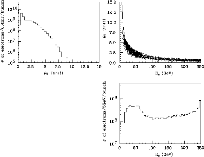
Figure 13.26: Scatter plot of disrupted electrons at $\sqrt{s_{e^{-}e^{-}}}=500$GeV, where the horizontal and vertical axes are the energy (E_e) and disruption angle ($\theta_{d}$), respectively. The solid line is a calculation by equation 13.36. Histograms projected on both axes are also shown.

The disruption angle can also be approximately expressed by

$$\theta_{d}\approx{Nr_{e}\over{\sqrt{2}\gamma(\sigma^{*}_{x}+\sigma^{*}_{y})}}\approx{94[{\rm mr}]\over{E_{e}[{\rm GeV}]}},$$ (13.36)

where $N$ and $r_{e}$ are the electron-beam intensity and the electron classical radius, respectively, and $\sigma^{*}_{x(y)}$ is the electron-beam size at the IP (see table 13.1). An analytic calculation a little bit overestimates the disruption angle compared to the simulation at low energy, while they agree with each other in the high-energy region, as shown in Fig. 13.26. The maximum disruption angle is about $10mr$, which corresponds to the electron energy of 10GeV.

Because of the large disruption angle, the crossing angle should be large for the disrupted electrons to pass through the nearest final focus magnet without any interaction. Therefore a crab-crossing scheme has to be necessary to avoid reduction of the luminosity.

The other source of backgrounds is low-energy $e^{+}e^{-}$  pairs produced by incoherent productions, such as Breit-Wheeler ($\gamma\gamma\to e^{+}e^{-}$), Bethe-Heitler ($\gamma e^{\pm}\to e^{\pm}e^{+}e^{-}$), and Landau-Lifshitz ($e^{+}e^{-}\to e^{+}e^{-}e^{+}e^{-}$). Since the mechanism of the pair creations is the same as that of the $e^{+}e^{-}$collision, the background in detectors should be similar to that at $e^{+}e^{-}$collision, where a detailed simulation result has been presented[39].

The low-energy particles are moving along the helical trajectories with a radius of $R=2\rho\sin\phi/2$, where $\rho=p_{t}/0.3B$ and $\phi=0.3Bz/p_{z}$ in a detector-solenoidal magnetic field of $B=$2T. Here, $z$ is the distance along the beam axis. Since they are created at very forward angles ($m_{e}/E_{e}$), they obtain their transverse momenta ($p_{t}$) mainly from deflections due to a strong electromagnetic field of the opposing beam. Their trajectories make a bundle along the beam axis. The boundary of the bundle is given by a particle with the maximum $p_{t}$, that is the maximum deflection angle. Any detectors and masks must be located outside of the bundle in order to avoid a huge background. There are also particles with inherently large scattering angles outside of the bundle; however since the number is relatively small, they can be tolerable, as mentioned below. The maximum deflection angle ($\theta_{max}$) can be expressed by

$$\theta_{max}=\theta_{\circ}\sqrt{2\ln(4\sqrt{3}D_{x}/\epsilon)/\sqrt{3}\epsilon D_{x}}~{},$$ (13.37)

where $\theta_{\circ}=D_{x}\sigma^{*}_{x}/\sigma^{*}_{z}$, $D_{x}=2r_{e}N\sigma^{*}_{z}/(\gamma\sigma^{*}_{x}(\sigma^{*}_{x}+\sigma^{*}_{y}))$ and $\epsilon=p/E_{beam}$. For the high energy $\gamma\gamma$collision, $D_{x}=$1.68 and $\theta_{\circ}=1.08mr$. Since $\theta_{max}$ is less than 0.2 for our cencerned particles, we can approximate $p_{z}\approx p$. Thus, $\phi$ is a function of $p$ alone. Apparently, the maximum radius is $R_{max}=2\rho$ at $\phi=\pi$, where $p_{max}=0.3Bz/\pi$. We therefore obtain $R_{max}$ as a function of $z$,

$$R_{max}\approx{2p_{max}\theta_{max}\over{0.3B}}={2z\theta_{max}\over{\pi}}.$$ (13.38)

For the innermost layer of the vertex detector with $z=\pm 5.2$ cm ($|\cos\theta|<$0.90 ), $R_{max}$ was calculated to be 1.6cm, which is smaller than the present $r_{vtx}$=2.5cm.

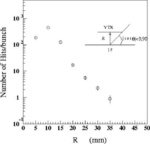
Figure 13.27: Expected number of background hits in tracking detectors per bunch crossing.

The number of background hits was actually calculated as a function of the radial distance (R) from the beam axis in the angular region $|\cos\theta|<$0.90 with no secondary interaction. The result is shown in Fig. 13.27. In the estimation, multiple hits were registered by a helical track. At $r_{vtx}$=2.5cm, the number of hits is about 10 per bunch crossing, that is O($10^{3}$) hits per pulse train. Since the number is indeed similar to that of the $e^{+}e^{-}$collision, a very similar environment of backgrounds is expected due to the pairs.

Secondary particles, which are back-scattered at the final focus magnet, are prevented from going into the detectors by a conical masking system.

The engineering level design of the interaction region including the laser optics and masking system are still under consideration. A design closest to the engineering level at this moment is shown in Fig. 13.28 which is found in [114].

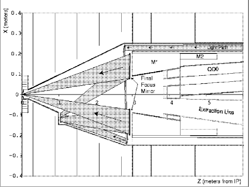
Figure 13.28: A schematic of the interaction region of the $\gamma\gamma$  collider  [114].

In this design, the aperture of the electron beam exaction line is about $10mr$ to accommodate the spent electrons and the beam crossing angle is enlarged to $30mr$ to avoid interference between the extraction line and the final focus magnet. The laser path is also shown in Fig. 13.28. The final focus mirror is mounted on the tungsten mask(M1) which is 3 m from the interaction point. The mirror is 38cm in diameter with a hole of 15 cm diameter for the electron lines. The detail description of this design is found in [114].

13.4.2 Lasers

Requirements for the laser system are shown in table 13.13. It is difficult to generate such a high-energy pulse and a complicated time structure by a single laser. One of the promising solutions is to build 95 lasers( 190 lasers in total for two linacs), which is a 190 laser system. In this case, each laser generates 1 J/pulse at 150 Hz. Key issues are

1. 1J pulse with 1 ps width

2. Synchronization of each pulse

3. Collision with beam-bunches and pulses

4. Focus and pointing stability

In this section, current and future technologies for the above issues are described.

Table 13.13: Requirements for the laser system

Time structure	a train of 95 pulses with 2.8 ns intervals
Repetition rate	150 Hz
Pulse energy	1 J
Pulse width	1 ps
Wavelength	1 $\mu$m
focusing spot size in diameter	3 $\mu$m (r.m.s)

1 J laser pulse with 1 ps pulse width

The rapid and remarkable progress of short pulse lasers has led to the demonstration of $>$ 1J femto-(pico-)second pulse.

A Nd:glass laser has been often used for high energy short pulse generation. However, its repetition rate is too low ($\leq$ 1 Hz) because of the poor thermal property. The other Nd-doped materials have been also used for high energy pulse lasers, but the pulses are not short enough for our purpose. Even in the low energy mode-locked oscillators, the shortest pulse has been obtained to be 2 ps (Nd:YLF) or 5 ps (Nd:YAG) [115].

One of realistic choices is to use Ti:sapphire crystals with a Chirped Pulse Amplification(CPA) systems [116]. The mode-locked oscillator can generate pulses as short as tens of femtosecond. These short pulses must be stretched in hundreds of picosecond or in a nanosecond, then a pulse is picked up by a Pockels cell to be amplified. Finally, the amplified pulse is compressed. Generally in the usual CPA system, it is compressed into the initial or slightly longer pulse. However, for a $\gamma\gamma$ collider, it is intended to be compressed insufficiently for the requirement of 1 ps pulse-width.

Problematic issues of the Ti:sapphire laser system are high cost, low reliability, short wavelength, and energy chirp in a pulse. High cost and low reliability come from the same reason. The pumping wavelength is around 500 nm, where Ar⁺ ion lasers or a second harmonics of Neodium doped lasers (e.g. crystals of Nd:YLF or Nd:YVO₄) are used as a pump source. Since Ar⁺ ion lasers are pumped by a discharge, the stability is too poor for a $\gamma\gamma$ collider. On the other hand, the Nd doped lasers are sufficiently stable since they can be pumped by laser diodes(LDs). Wavelength of the Nd lasers must be reduced to half in the second harmonics. In this case, a pumping scheme is much more complicated than that without the wavelength conversion. Generally, a complicated scheme has high cost and low reliability which may cause a serious problem in the 190 laser system. Wavelength of Ti:sapphire laser is around 800 nm which is shorter than the required wavelength of $1\mu$m. The insufficient compression leaves residuals of energy chirp. Therefore the wavelength varies about 5% (40-50 nm in 800 nm) in a pulse.

Nevertheless, the Ti:sapphire CPA system is an influential candidate, since the technology has been well established. The required specifications, except for the wavelength, for the $\gamma\gamma$ collider can be constructed using existing technologies. Additionally, due to the wide spectral bandwidth, square temporal profiles can be generated using a spatial light module (SLM). The laser power can be constant in the pulse [118].

Another possibility is to use a crystal of Ytterbium doped with Sr₅(PO₄)₃F (Yb:S-FAP) [119]. The laser wavelength is 1047 nm consistent with the required specification. The spectral bandwidth is sufficiently wide and seems to be good for sub picosecond or 1 ps pulses. It can be directly pumped by LDs. Furthermore, the upper state lifetime is 1.2 ms, which is five times longer than Nd:YAG and 2.5 times longer than Nd:YLF. Fewer LDs are required to produce the same energy output because the pumping energy can be stored in the crystal over a longer period of time. Comparing to the Ti:sapphire crystal with Nd doped laser(second harmonic), the Yb:S-FAP crystals have advantages of reduced cost and improved reliability. Yb:S-FAP crystals do not require another laser as a pumping source nor frequency conversion. The total system is much simpler and the required pumping energy is one order of magnitude less than the Ti:sapphire laser. One the other hand, the Yb:S-FAP crystals have not been well investigated. Further research is required to determine if this crystal can generate 1 ps pulses.

Timing synchronization of each laser pulse

The synchronization of 190 lasers is one of the most important technologies in the 190 laser system, where each pulse must be synchronized to the electron beam bunch. It is not realistic to measure the electron timing for a feedback to the laser system because the electron pulses travel at almost the speed of light and the time to feedback is too short. The laser pulses must be synchronized to the RF signal which drives the linacs. Then the laser pulses can be synchronized to the electron pulses. In order to achieve the synchronization, three stages will be built.

The first stage is the synchronization of a mode-locked master oscillator. Either for Ti:sapphire or Yb:S-FAP, a single oscillator will be used as an injection seeder for all amplifiers. The pulse timing of mode-locked oscillator can be adjusted by the optical length of the laser cavity. So, the oscillator can be synchronized to the RF signal with a conventional phase locking technique by adjusting the position of the cavity mirror. The synchronization of less than 100 femtosecond has been already demonstrated [120].

The second stage is the pulse divider. The repetition rate of the oscillator should be 357 MHz (2.8 ns interval). Using high-speed Pockels cells, 95 laser pulses are picked up and divided into 95 beams. The timing of the drive signal for each Pockels cell is not critical because it is used only for the ”gate signal”. The accuracy is determined by the mode-locked oscillator. Finally, each picked pulse is divided into two by a beam splitter and delivered to the amplifiers for two linacs. The series of Pockels cells and the timing structure are shown in Fig.13.29 and Fig.13.30, respectively.

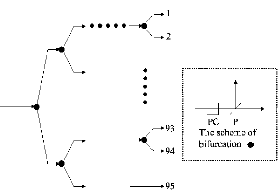
Figure 13.29: Pulse divider, consist of the series of Pockels cells. The scheme of bifurcation is shown in the dotted box. PC: Pockels cell, P: thin film polarizer or Grand Thomson prism.

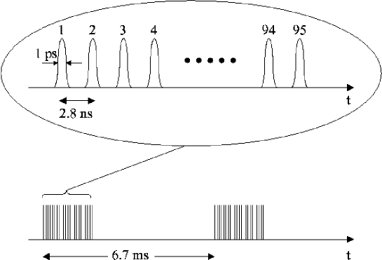
Figure 13.30: The timing structure of the laser pulses.

The third stage is the stabilization of the amplified pulses. The amplified pulses are automatically synchronized in principle because the injected seed pulses are synchronized to the RF signal. However, a stabilization is still required because additional disturbances may induce fluctuations. One example of such disturbances is the thermal expansion. Since the laser pulses travel in a long distance, the arriving time to the colliding point may fluctuate. The other is the mechanical vibration. Vibrations of the beam delivering mirrors cause a change in the optical pass length. The repetition rate of each amplifier is 150 Hz. A statistical technique cannot be applied to measure the fluctuation because of the low repetition rate, while it can be applied for the mode-locked oscillator. An elegant method to measure and stabilize the amplified pulses has already been demonstrated [121]. In this method, stabilized oscillator pulses are used as a reference and the timing lag between the oscillator pulse and the amplified pulse is measured by a modified cross-correlation technique. Using this technique, sub femtosecond stabilization has been achieved.

Collision between the beam-bunch and the laser pulse

Since 95 optical amplifiers will be required for each linac, Collision between the beam-bunch and the laser pulse is an important issue. The laser pulses shall be focused by 95 different angles to a colliding point, where 95 optical mirrors must be placed on the base of a cone whose tip is the collision point. Instead of the 95 mirrors, a single parabola reflector can be used too. The advantage of this method is a simplicity. We can align the path of each laser pulse independently. On the other hand, it occupies a large space. Also, each amplifier requires a pulse compressor.

Another solution is to combine the pulses using Pockels cells. Reverse procedure of pulse divider for the oscillator can be applied. But this time, the energy of the amplified pulse is much higher than that of the oscillator. To avoid optical damage, pulse diameter should be very large. It is necessary to develop a large aperture, high damage threshold, and high-speed ($\geq$ 357 MHz) Pockels cell. If such a Pockels cell can be developed, every pulse can be co-axially overlapped. After overlapping, only one compressor and one focusing mirror are required.

Tight focus and pointing stability

The tight focus and pointing stability of the amplified laser pulses is a key issue for the stable collisions. In general, the thermal problem is the biggest issue in high energy laser amplifiers. Inhomogeneous thermal distributions result in wave-front distortions [122, 123] and then the focus becomes poor. Also, the fluctuations of the thermal distributions lead to pointing instabilities.

There are two choices to compensate for the inhomogeneous thermal distributions. One is to use a phase-conjugation mirror such as SBS cell. But the reflectivity is not very high, and it requires much bigger amplifiers to obtain sufficient energy.

The another choice is to use adaptive optics (deformable mirrors). First order wave-front distortions can be removed using a telescope [124]. Remaining distortions will be measured using a Shack-Hartmann type wave-front sensor  [125], and adaptive optics will be used to remove the distortion. To reduce the pointing instability, a set of mirrors will be used as a vector scanning system. Figure 13.31 shows the set of adaptive optics and vector scanning mirrors.

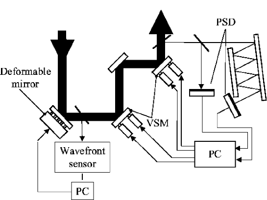
Figure 13.31: Wave-front correction and the pointing stabilization. PC: personal computer, VSM: vector scanning mirror, PSD: position sensitive detector.

Summery of the laser system

In this section, a laser system for the $\gamma\gamma$ collider is proposed. The basic idea is to build an amplifier for each pulse, and combine the pulses with synchronizing technique. This system can be built, in principle, with the state of the art Ti:sapphire laser technology. However, the cost is expected to be very high, and the reliability may not be sufficient. We have enough time to develop a next generation laser system. The key technologies are picosecond pulse amplification with Yb:S-FAP crystals and the beam combination with large aperture Pockels cells. Figures 13.32 and 13.33 show the proposed laser system. Figure 13.32 is the oscillator stage, consisting of a mode-locked oscillator, synchronization circuit to RF reference signal, pulse stretcher, and pulse divider. Figure 13.33 is the amplifier stage. 95 amplifier stages (total 190 amplifiers for two linacs) will be built. The amplified pulses will be delivered to the interaction region with 95 different paths or a single path after beam combination by a series of Pockels cells.

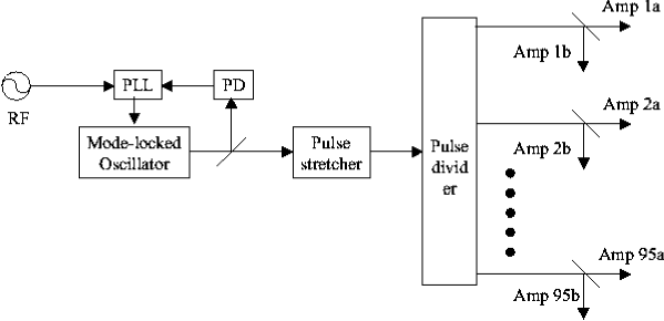
Figure 13.32: The oscillator stage of the laser system.

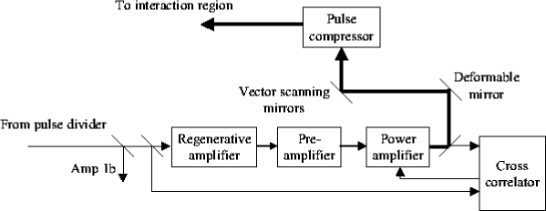
Figure 13.33: The amplifier stage of the laser system.

One of the most unknown part of above laser system is the way of laser pulse combination, i.e., how it is possible to deliver 95 laser path from deferent path to each electron bunch. A method is to install 95 mirrors at the interaction region but seems to be impossible because there is no space available. The other way is to combine pulses from different paths to pulse train by Pockels cell before entering the interaction region. However, the development of required high power and fast Pockels cell are issue to be solved.

The NLC group proposed different idea for the laser scheme based on Mercury laser system[126]. The Mercury laser is 100J/pulse, 10Hz with 2-10ns pulse length which is now under development at LLNL. The idea to avoid the problem of pulse combination is that a pulse train consists of 95 pulses with 2.8 ns spacing is formed before the amplification. Each pulse is chirped and overlapped temporarily so that the envelop is a $\approx 300ns$ pulse. However each pulse can still be identified because they are not overlapped in frequency. After amplification by the Mercury amplifier, the pulses are compressed to 95 of 1ps pulses. Since the Mercury laser is design to operate 10Hz, it only needs 12 systems to provide the laser pulses to ${\rm 95\times 120Hz}$ electron bunches.

13.5 Summary and Future Prospect

According to the studies in the last decade, the characteristics of the beams provided by the $\gamma\gamma$and the $e\gamma$collider and overall view of the physics opportunities have been clear. It has been shown that $\gamma\gamma$  and the $e\gamma$  colliders using backward Compton scattering could provide comparable luminosity with the $e^{+}e^{-}$collider as well as have unique feature of providing polarized photon beams. It also has many good physics opportunities, some of which are unique and only possible with these facilities and some of which are complementary to the $e^{+}e^{-}$interaction.

Regarding these aspects, the R&D efforts are now tuning in to reveal feasibility of the $\gamma\gamma$  and $e\gamma$  collider as realistic as possible in both physics and technical aspect. In the physics study, we need simulation study by taking into account the realistic luminosity distribution and the detector performance. In the technical aspect, continuous effort for the development of the laser and design of the interaction region is the key issue for the realization of the $\gamma\gamma$  and $e\gamma$  colliders. However, looking at the manpower available, we understand the world wide level collaboration is very importance to perform these R&D effort effectively. For this purpose, we are now organizing an international working group including Asia, North America and European region and started a real collaborative work with the North America group for the design of the interaction region.

We believe that the feasibility of the $\gamma\gamma$  and $e\gamma$  collider will be clear as the same level as is in the $e^{+}e^{-}$collider for now in a couple of years and is possible to put it on a part of the linear collider project.

Acknowledgement

Many topics described in this chapter are based on discussions and/or works in the international collaborative group on the $\gamma\gamma$  and $e\gamma$  collider. The author would like to thank all participants of the collaboration in the North America and Europe. Particularly, we thank colleagues in the Lawrence Livermore National Laboratory for providing us materials on the interaction region and the laser sections.

Acknowledgements

This work is supported in part by the following organizations/programs: Japan Society for the Promotion of Science (JSPS), -JSPS-CAS Scientific Cooperation Program under the Core University System, -JSPS Japanese-German Cooperative Program, -Japan-US Cooperative Program in High Energy Physics; Foundation for High Energy Accelerator Science; The Australian Research Council (ARC) and The Department of Industry, Science & Resources (DISR); Commission on Higher Education of the Philippines.

Appendix A ACFA Statement

Statement Of Physics Study Group On The $e^{+}e^{-}$ Linear Collider

On the 2nd plenary meeting, ACFA announced its endorsement of the e+e- linear collider as one of the major future facilities in the Asia-Pacific region. In fact, recent world-wide research at existing facilities has enabled us to form a more and more concrete picture of ”TeV-scale physics” and, consequently, has made the $e^{+}e^{-}$ linear collider’s role more and more crucial in its exploration. According to the recent picture, the linear collider is expected to produce very important, decisive physics outputs even in the initial stage (in the energy region below 500GeV) of its energy upgrading program ; for instance, a top quark study at threshold, which is very important in its own right, can be a key to new physics and, more importantly, the Higgs particle will almost certainly manifest itself there or the SUSY/GUTS scenario will be disapproved.

In addition to its role as an energy frontier machine for High Energy Physics, the linear collider has a facet which can be shared with a new means for materials science. The ultra-low emittance beam essential to the linear collider is also an indispensable element of the next-generation, coherent x-ray source. In order to efficiently and effectively promote accelerator science in the region, one should start seriously thinking about the possibility of integrating both into a single project.

Turning our attention to activities in Asian region, we see significant progress in high energy and synchrotron radiation experiments at various domestic facilities. Not only that, many researchers from ACFA member nations are actively participating in large-scale experiments such as at LEP-II, Tevatron collider, HERA and PEP-II/KEKB. The Asian physics community on which ACFA is based has grown significantly and has set a firm enough foundation to prepare for further advancement.

In response to the ACFA statement issued in the last year, considering the importance of the linear collider project and the potential of our community to realize it, we agreed to set up a study group under ACFA. The charge of the group should be to elucidate physics scenario and experimental feasibilities and to write up a report to ACFA within two years. Taking account of the scale of and the world-wide interests in such project, actual studies shall hopefully be carried out in a more global scope in spite of the regional nature of ACFA’s initiative.

July 22, 1998
Zhipeng Zheng
Chairman, Asian Committee for Future Accelerators
Director, Institute of High Energy Physics,
Chinese Academy of Sciences

Bibliography

- [1] The ACFA statement is attached in the Appendix; See also the working group home page http://acfahep.kek.jp/ and the ACFA home page http://www.acfa-forum.net/.
- [2] The proceedings of workshops and meetings held in the past few yeards are as follows; The proceedings of the First ACFA Workshop on Physics and Detector at the Linear Collider, Tsinghua University, Beijin, ed. Takayuki Matsui and Yu-Ping Kuang, KEK Proceedings 99-12, September 1999; Second ACFA Workshop, http://acfalc99.korea.kr.ac/; ACFA-LC3, in the Proceedings of the 8th ASIA-Pacific Physics Conference (APPC2000), August 2000, Taipei, ed. Yeong-Der Yao, Hai-Yang Cheng, Chia-Seng Chang, Shang-Fan Lee, (World Scientific, 2001); The Proceedings of the APPI Winter Institute, APPI, Feburary 2001, ed. Yoshiaki Fujii, KEK Proceedings 2001-16, August 2001; The Proceedings of the KEK theory meeting on Physics at Linear Colliders 15–17 March 2001, KEK, ed. K. Hagiwara and N. Okamura; See also http://acfahep.kek.jp/.
- [3] JLC-I, JLC Group, KEK Report 92-16, December 1992.
-
[4]
S. Weinberg, Phys. Rev. Lett. 19 (1967) 1264;
A. Salam, Proc. 8th Nobel Sympos., Stockholm, ed. by N. Svartholm (Almqvist and Wiksell, Stockholm, 1968) p. 367. - [5] CDF collaboration, Phys. Rev. Lett. 74 (1995) 2626; D0 collaboration, Phys. Rev. Lett. 74 (1995) 2632.
- [6] LEP collaboration, Phys. Lett. B276 (1992) 247.
- [7] Super-Kamiokande Collaboration, Phys. Rev. Lett. 81 (1998) 1562.
- [8] See, for instance, P. Ramond, hep-ph/0106129.
-
[9]
Y. Nambu and G. Jona-Lasinio, Phys. Rev. 122
(1961) 345;
P.W. Higgs, Phys. Lett. 12 (1964) 132, Phys. Rev. 145 (1966) 1156. -
[10]
UA1 Collaboration, Phys. Lett. 122B (1983) 103,
126B (1983) 398;
UA2 Collaboration, Phys. Lett. 122B (1983) 476; 129B (1983) 130. - [11] The LEP Collaboration ALEPH, DELPHI, L3, OPAL, the LEP Electroweak Working Group and the SLD Heavy Flavour and Electroweak Group, CERN-EP/2001-021 and hep-ex/0103048. Status of winter 2001: LEPEWWG/2001-01; LEP Electroweak Working Group report, CERN-EP-200-016 (January 21, 2000).
-
[12]
P. Igo-Kemenes for LEP Higgs Working Group, presentation given to
the LEP Experiments Committee open session,
http://lephiggs.web.cern.ch/LEPHIGGS/talks/index.html, 3 November 2000;
ALEPH Collaboration, R. Barate et al., Phys. Lett. B495 (2000) 1;
L3 Collaboration, M. Acciarri et al., Phys. Lett. B495 (2000) 18;
DELPHI Collaboration, P. Abreu et al., Phys. Lett. B499 (2001) 23;
OPAL Collaboration, G. Abbiendi et al., Phys. Lett. B499 (2001) 38. - [13] I. Nakamura and K. Kawagoe, Phys. Rev. D 54 (1996) 3634.
-
[14]
D.V. Volkov and V.P. Akulov, Phys. Lett. 46B
(1973) 109;
J. Wess and B. Zumino, Nucl. Phys. B70 (1974) 39. -
[15]
M. Veltman, Acta Phys. Pol. B12 (1981) 437;
L. Maiani, Proc. Summer School of Gil-sur-Yvette (Paris, 1980) p. 3. - [16] R. Barbieri and G.F. Giudice, Nucl. Phys. B306 (1988) 63; G.G. Ross and R.G. Roberts, Nucl. Phys. B377 (1992) 571; B. de Carlos and J.A. Casas, Phys. Lett. B309 (1993) 320; G.W. Anderson and D.J. Castaño, Phys. Rev. D52 (1995) 1693; K.L. Chan, U. Chattopadhyay, and P. Nath, Phys. Rev. D58 (1998) 096004; J.L. Feng, K.T. Matchev, and T. Moroi, Phys. Rev. Lett. 84 (2000) 2322, Phys. Rev. D61 (2000) 075005.
- [17] L. Randall., and R. Sundrum, Nucl. Phys. B 557, 79 (1999), hep-th/9810155; G.F. Giudice, M.A. Luty, H. Murayama, and R. Rattazi, JHEP 27, 9812 (1998), hep-ph/9810442.
- [18] M. Dine, A.E. Nelson and Y. Shirman, Phys. Rev. D 51, 1362 (1995), hep-ph/9408384; M. Dine, A.E. Nelson, Y. Nir, and Y. Shirman, Phys. Rev. D 53, 2658 (1996), hep-ph/9507378.
- [19] T. Tsukamoto, K. Fujii, H. Murayama, M. Yamaguchi, and Y. Okada, Phys. Rev. D51 (1994) p3153.
- [20] M. Nojiri, K. Fujii, and T. Tsukamoto, Phys. Rev. D54 (1996) p6756.
- [21] Schmaltz, M., and Skiba, W., Phys. Rev. D 62, 095004 (2000), hep-ph/0004210; Phys. Rev. D 62, 095005 (2000), hep-ph/0001172; Chacko, Z., Luty, M.A., Nelson, A.E., and Ponton, E., JHEP 1, 3 (2000), hep-ph/9911323.
- [22] H. Georgi and S. Glashow, Phys. Rev. Lett. 32 (1974) 438.
-
[23]
K. Inoue, A. Kakuto, H. Komatsu and S. Takeshita, Prog. Theor. Phys. 68 (1982) 927;
L.E. Ibanez and G.G. Ross, Phys. Lett. 110B (1982) 215;
K. Inoue, A. Kakuto and S. Takeshita, Prog. Theor. Phys. 71 (1984) 348;
L. Alvarez-Gaumé, J. Polchinski and M.B. Wise, Nucl. Phys. B221 (1983) 495;
J. Ellis, J.S. Hagelin, D.V. Nanopoulos and K. Tamvakis, Phys. Lett. 125B (1983) 275. - [24] See E. Farhi and L. Susskind, Phys. Rep. 74 (1981) 277, and references therein.
- [25] K. Fujii, T. Matsui and Y. Sumino, Phys. Rev. D50, 4341 (1994);
- [26] V.S. Fadin and V.A. Khoze, JETP Lett. 46, 525 (1987); Sov. J. Nucl. Phys. 48, 309 (1988).
- [27] I. Antoniadis, Phys. Lett. B246 (1990) 377; J.D. Lykken, Phys. Rev. D54 (1996) 3693; N. Arkani-Hamed, S. Dimopoulos, and G. Dvali, Phys. Lett. B429 (1998) 263; L. Randall and R. Sundrum, Phys. Rev. Lett. 83 (1999) 3370.
- [28] See for instance, S. Riemann, Proceedings of LCWS 2000, Batavia, Illinois, (2000) 619.
- [29] H. Yamamoto, Proc.of the 4th International Workshop on Physics and Experiments with Future Linear Colliders, April 1999, Sitges, Spain
- [30] R.J.Wilson, Proc.of the 4th International Workshop on Physics and Experiments with Future Linear Colliders, April 1999, Sitges, Spain
- [31] JLC Design Study, KEK Report 97-1, Aprril 1997.
- [32] International Study Group Progress Report on Linear Collider Development, KEK-SLAC International Study Group on Linear Colliders, April 2000. KEK Report 2000-7, SLAC-R-559. Available at http://lcdev.kek.jp/ISG/.
- [33] http://lcdev.kek.jp/ for X-band and http://c-band.kek.jp/ for C-band.

Bibliography

- [1] P.W. Higgs, Phys. Lett. 12 (1964) 132; F. Englert and R. Brout, Phys. Rev. Lett. 13 (1964) 321; G.S. Guralnik, C.R. Hagen, and T.W.B. Kibble, Phys. Rev. Lett. 13 (1964) 585.
-
[2]
S. Glashow, Nucl. Phys. 22 (1961) 579;
S. Weinberg, Phys. Rev. Lett. 19 (1967) 1264;
A. Salam, ed. N. Svartholm, Elementary Particle Theory, Almquist and Wiksells, Stockholm (1968) 367. -
[3]
P. Igo-Kemenes for LEP Higgs Working Group, presentation given to
the LEP Experiments Committee open session,
http://lephiggs.web.cern.ch/LEPHIGGS/talks/index.html, 3 November 2000;
ALEPH Collaboration, R. Barate et al., Phys. Lett. B495 (2000) 1; L3 Collaboration, M. Acciarri et al., Phys. Lett. B495 (2000) 18; DELPHI Collaboration, P. Abreu et al., Phys. Lett. B499 (2001) 23; OPAL Collaboration, G. Abbiendi et al., Phys. Lett. B499 (2001) 38. - [4] Sun Kee Kim, Recent results from Tevatron, KEK report 99-12 (1999), the proceedings of the ACFA Workshop on Physics and Detector at the Linear Collider, Beijing, China, Nov. 1998; J. Conway, Higgs Discovery Potential in Run 2 at the Tevatron, in Proceedings of LCWS’99, Apr-May 1999, Sitges, Spain.
- [5] See for example; M. Carena, et al., CERN-TH-99-203, Jul 1999. 35, hep-ph/9907422; S. Abdullin et al., Phys. Lett. B431 (1998) 410, hep-ph/9805341; Z. Kunszt et al., Z. Phys. C74 479-491 (1997), hep-ph/9611397. S. Moretti, hep-ph/9612310, and their references.
- [6] H.P. Nilles, Phys. Rep. 110 (1984) 1; H.E. Haber and G.L. Kane, Phys. Rep. 117 (1985) 75; R. Barbieri et al., Z Physics at LEP1, CERN 89-08, Vol. 2, 121; J.M. Frère and G.L. Kane, Nucl. Phys. B223 (1983) 331; J. Ellis et al., Phys. Lett. B123 (1983) 436; J. Ellis et al., Phys. Lett. B127 (1983) 233.
-
[7]
Searches for Higgs bosons: preliminary combined results using
LEP data collected at energies up to 202 GeV,
ALEPH, DELPHI, L3, OPAL Collaborations, LEP working group
for Higgs boson searches, P.Bock et al., CERN-EP-2000-055, 25 Apr 2000,
Presented at 35th Rencontres de Moriond on Electroweak
Interactions and Unified Theories, Les Arcs, France, 11 - 18 Mar 2000;
Chang-Gen Yang, Recent results from LEP – Precision EW, KEK report 99-12 (1999), the proceedings of the ACFA Workshop on Physics and Detector at the Linear Collider, Beijing, China, Nov. 1998; Atul Gurtu, Recent results from LEP – New Particle Searches, KEK report 99-12 (1999), the proceedings of the ACFA Workshop on Physics and Detector at the Linear Collider, Beijing, China, Nov. 1998; S. Komamiya LEP-II Physics, prodeedings of the 3rd ACFA workshop, APPC’00, Taipei, 2000. - [8] The LEP Collaboration ALEPH, DELPHI, L3, OPAL, the LEP Electroweak Working Group and the SLD Heavy Flavour and Electroweak Group, CERN-EP/2001-021 and hep-ex/0103048. Status of winter 2001: LEPEWWG/2001-01; LEP Electroweak Working Group report, CERN-EP-200-016 (January 21, 2000).
- [9] The OPAL Collaboration, G. Abbiendi et al., Eur. Phys. J. C18 (2001) 425-445.
- [10] The BES Collaboration, G-P. Chen et al., Nucl. Phys. A675 (2000) 112-115.
-
[11]
J. Kamoshita, Y. Okada, M. Tanaka, Phys. Lett. B328 (1994) 67;
T. Moroi, Y. Okada, Phys. Lett. B295 (1992) 73. - [12] J.R. Espinosa, M. Quiros, Phys. Rev. Lett. 81 (1998) 516; J.R. Espinosa and J.F. Gunion, Phys. Rev. Lett. 82 (1999) 1084.
- [13] S. Yamashita, Higgs at Future e+e- Linear Collider, KEK Proceedings 99-12 (1999), The ACFA Workshop on Physics and Detector at the Linear Collider, Beijing, China, Nov. 1998.
- [14] S. Yamashita, Higgs at JLC-I, presented at the 3rd ACFA Workshop on Physics and Detector at the Linear Collider, Taipei, Aug. 2000.
- [15] S. Yamashita, HIGGS AT FUTURE LINEAR COLLIDER, in Proceedings of LCWS’99, Apr-May 1999, Sitges, Spain.
-
[16]
See for example;
N. Akasaka et al., JLC DESIGN STUDY, KEK-REPORT-97-1 (1997) 617;
JLC Group, JLC-I (the green book), KEK-REPORT-92-16 (1992);
Web page http://www-jlc.kek.jp/ - [17] See for example; T. Matsui, JLC Detector Overview, in Proceedings of LCWS’99, Apr-May 1999, Sitges, Spain. T. Tauchi, Detector Overview, proceedings of the 3rd ACFA workshop, APPC’00, Taipei, 2000.
-
[18]
A. Miyamoto, JSF,
in Proceedings of
LCWS’99, Apr-May 1999, Sitges, Spain.
Web page; http://acfahep.kek.jp/subg/sim/ - [19] Web page; http://www-jlc.kek.jp/subg/offl/jim/index-e.html
- [20] I. Ueda, Effects of the Beamstrahlung, in Proceedings of LCWS’99, Apr-May 1999, Sitges, Spain.
- [21] V.N. Baier and K. Yokoya, Interaction of high energy electrons and photons with intense electromagnetic wave: linear collider applications (28 pages), submitted to Particle Accerelators. K. Yokoya and P. Chen, Beam-beam phenomena in linear colliders, Frontiers of Particle Beams: Intensity Limitations, edited by M.Month and S.Turner, Lecture Notes in Physics Vol. 400, 415-445; T. Tauchi, K. Yokoya and P. Chen, Particle Accerelators 41 (1993) 29-39.
- [22] J. Kanzaki and S. Yamashita, Effects of Beam-beam Interaction, Event-Overlap in Higgs Measurements, in Proceedings of LCWS’99, Apr-May 1999, Sitges, Spain.
- [23] Y. Okada, M. Yamaguchi, T. Yanagida, Phys. Lett. B262 (1991) 54.
- [24] M. Carena, S. Mrenna, and C.E.M. Wagner, Phys. Rev. D60 (1999) 075010; K.S. Babu and C. Kolda, Phys. Lett. B 451 (1999) 77; H. Eberl, K. Hidaka, S. Kraml, W. Majerotto, and Y. Yamada, Phys. Rev. D62 (2000) 055006; M. Carena, D. Garcia, U. Nierste, and C.E.M. Wagner, Nucl. Phys. B 577 (2000) 88; H.E. Haber, M. Herrero, H.E. Logan, S. Peñaranda, S. Rigolin, and D.Temes, Phys. Rev. D63 (2001) 055004.
- [25] T. Moroi, and Y. Okada, Phys. Lett. B 295 (1992) 73.
- [26] HIGGS PHYSICS AT LEP-2, in CERN LEP-2 yellow report vol.1, CERN-96-01, hep-ph/9602250; W. Kilian, M. Kramer, P.M. Zerwas, Phys. Lett. B373 (1996) 135.
- [27] See for example; T. Omori, A Polarized Positron Beam for Linear Collider, KEK-PREPRINT-98-237, 1999, The 1st ACFA Workshop on Physics/Detector at the Linear Collider Tsinghua University, Beijing, The People’s Republic of China, Nov 26 - 27, 1998.
-
[28]
T. Omori, Y. Kurihara, Y. Sugimoto, Y. Fujii, K. Fujii,
KEK-Proc.-94-01, 102-111.
T. Omori, Proceedings of LCWS93, Waikoloa, Hawaii (1993) 791; - [29] K. Ishii, Detector Acceptance and CAL Resolution Requirements for HZ/WW-fusion Cross-section Measurements, in Proceedings of LCWS’99, Apr-May 1999, Sitges, Spain.
- [30] J. Kamoshita, Y. Okada, M. Tanaka, Phys. Lett. B391 (1997) 124.
- [31] I. Nakamura and K. Kawagoe, Phys. Rev. D 54 (1996) 3634.
- [32] M.D. Hildreth et al., Phys. Rev. D 49 (1994) 3441
- [33] T. Tauchi and H. Hayashii, Proceedings of LCWS93, Waikoloa, Hawaii, 26-30 April 1993, p745, KEK-preprint 93-105.
- [34] Allister Levi C. Sanchez, et al, talk presented 3rd ACFA workshop, August, 2000, http://acfahep.kek.jp/subg/sim/memo/0007-allister-higgs6jets.ps.gz; Jingle B. Magallanes, et al, talk presented APPI workshop, Feburary, 2001, http://www-jlc.kek.jp/miyamoto/export/Jingle-APPI.ps.gz
- [35] D. Zeppenfeld, R. Kinnunen, A. Nikitenko, and E.Richiter-Wa̧s, Phys. Rev. D 62 (2000) 013009.
- [36] M.M. Nojiri, Phys.Rev. D 51 (1995) 6281; M.M. Nojiri, K. Fujii, T. Tsukamoto, Phys.Rev. D 54 (1996) 6756.
- [37] J.L. Feng and T. Moroi, Phys. Rev. D 56 (1997) 5962; V.Barger, T. Han, and J.Jaing, Phys. Rev. D 63 (2001) 075002.
- [38] T. Tsukamoto, K. Fujii, H. Murayama, M. Yamaguchi, Y. Okada, Phys.Rev. D 51 (1995) 3152; J.L. Feng, M.E. Peskin, H. Murayama, X. Tata, Phys.Rev. D 52 (1995) 1418; S.Y. Choi, A. Djouadi, H. Dreiner, J. Kalinowski, P.M. Zerwas, Eur.Phys.J. C 7 (1999) 123; S.Y. Choi, A. Djouadi, H.S. Song, P.M. Zerwas, Eur.Phys.J. C 8 (1999) 669; S.Y. Choi, A. Djouadi, M. Guchait, J. Kalinowski, H.S. Song, P.M. Zerwas, Eur.Phys.J. C 14 (2000) 535.
- [39] K. Yokoya and T. Tauchi, ABEL (Analysis of Beam-beam Effects in Linear colliders) program.
- [40] S. Kanemura, K. Odagiri et al., Single production of charged Higgs bosons at linear colliders, LCWS’00 Proceedings, FNAL, US, 2000.

Bibliography

-
[1]
R. Barbieri and G. Giudice, Nucl. Phys. B296 (1988) 75;
T. Kon and M. Jimbo, Proceedings of the First Workshop on Japan Linear Collider, KEK, 1989, ed. by S. Kawabata, KEK Report 90-2, April, 1990, p.280;
K. Inoue, M. Kawasaki, M. Yamaguchi, and T. Yanagida, Phys. Rev. D45 (1992) 328. - [2] JLC-I (the green book), JLC Group, KEK Report 92-16 (1992).
- [3] For recent review, see for instance R.M. Godbole, plenary talk given at LCWS2000, October 26-30, 2000, Fermilab, hep-ph/0102191
- [4] R.M. Godbole, working group summary presented at III ACFA Linear Collider Workshop, August 9-11, 2000, Taipei, hep-ph/0011236
- [5] Randall, L., and Sundrum, R., Phys. Rev. Letters 83, 3370 (1999), hep-ph/9905221; ibid, 4690 (1999), hep-th/9906064.
- [6] Randall, L., and Sundrum, R., Nucl. Phys. B 557, 79 (1999), hep-th/9810155.
- [7] Giudice, G.F., Luty, M.A., Murayama, H., and Rattazi, R., JHEP 27, 9812 (1998), hep-ph/9810442.
- [8] Dine, M., Nelson, A.E., and Shirman, Y., Phys. Rev. D 51, 1362 (1995), hep-ph/9408384; Dine, M., Nelson, A.E., Nir, Y., and Shirman, Y., Phys. Rev. D 53, 2658 (1996), hep-ph/9507378.
- [9] Schmaltz, M., and Skiba, W., Phys. Rev. D 62, 095004 (2000), hep-ph/0004210; Phys. Rev. D 62, 095005 (2000), hep-ph/0001172; Chacko, Z., Luty, M.A., Nelson, A.E., and Ponton, E., JHEP 1, 3 (2000), hep-ph/9911323.
- [10] Peskin, M. E., hep-ph/0002041, Concluding lecture at the International Europhysics Conference on High Energy Physics, July 1999, Tampere, Finland.
- [11] Pierce, D., and Papodopoulos,A., Nucl. Phys. B 430, 278 (1994), hep-ph/9403240; Gherghetta, T., Giudice, G.F., and Wells, J.D., Nucl. Phys. B 559, 27 (1999), hep-ph/9904378.
- [12] CMS Technical Proposal, CERN/LHCC/94-38(1994); ATLAS Technical Proposal CERN/LHCC/94-43(1994).
- [13] ATLAS Technical Design Report 15, CERN/LHCC/99-14 and 15 (1999).
- [14] See for example, Hinchliffe, I., Talk presented at the Fermilab ‘Circle Line Tour’, http://www-theory.fnal.gov/CircleLine/IanBG.html; Polesello, G., Talk presented at SUSY2K June, 2000, http://wwwth.cern.ch/susy2k/susy2kfinalprog.html.
- [15] Godbole, R.M., hep-ph/0011237, In Proceedings of the 8th Asia Pacific Physics Conference, Taipei, Taiwan, Aug. 2000.
- [16] Barbieri, R., and Giudice, G.F., Nucl. Phys. B 306, 63 (1988).
- [17] Anderson, G.W., and Castaño, D.J., Phys. Rev. D. 52, 1693 (1995),hep-ph/9412322; Anderson, G.W., and Castaño, D.J., Phys. Rev. D. 53, 2403 (1996),hep-ph/9509212.
- [18] Feng, J.L, Matchev, K.T., and Moroi, T., Phys. Rev. Lett. 84, 2322 (2000),hep-ph/9908309; Feng, J.L., and Moroi, T., Phys. Rev. D 61, 095004 (2000), hep-ph/9907319.
- [19] See for example, Baer, H., Chen, C., Paige, F., and Tata, X., Phys. Rev. D 52, 2746 (1995), hep-ph/9503271; Phys. Rev. D 53, 6241 (1996), hep-ph/9512383
- [20] Hinchliffe, I., Paige, F.E., Shapiro, M.D., Soderquist, J., and Yao, W., Phys.Rev.D 55, 5520 (1997), hep-ph/9610544.
- [21] See for example Ref. [13] and references therein.
- [22] Bachacou, H., Hinchliffe, I., and Paige, F.E., Phys. Rev. D 62, 015009 (2000), hep-ph/9907518; Paige, F.E., hep-ph/9909215, Proceedings of LCWS99, Sitges, Spain, April 1999.
- [23] Drees, M., Kim, Y.G., Nojiri, M.M., Toya, D., Hasuko, K., and Kobayashi, T., Phys. Rev. D 63, 035008 (2001), hep-ph/0007202.
- [24] Baer, H., Munroe, R., and Tata, X., Phys. Rev. D 54, 6735 (1996), hep-ph/9606325, Erratum: ibid. 56, 4424 (1997).
- [25] See for instance, J. Grivaz, DESY 92-123B p663; R. Becker and C. Vander Velde, DESY 92-123C p457.
- [26] K. Hikasa, “JLC Supersymmetry Manual”, in preparation.
- [27] T. Tsukamoto, KEK Preprint 92-34, May, 1992.
- [28] T. Tsukamoto, K. Fujii, H. Murayama, M. Yamaguchi, and Y. Okada, Phys. Rev. D51 (1994) p3153.
- [29] Choi, S.Y., Djouadi, A., Guchait, M., Kalinowski, J., Song, H.S., and Zerwas, P.M., Eur. Phys. J C 14, 535 (2000), hep-ph/0002033; Choi, S.Y., Guchait, M., Kalinowski, J., and Zerwas, P.M., Phys. Lett. B 479, 235 (2000), hep-ph/0001175.
- [30] G. Blair and H.U. Martyn, hep-ph/9910416.
- [31] J. Feng, M. Peskin, H. Murayama, and X. Tata, Phys.Rev. D52 (1995) p1418.
- [32] H. Baer, R. Munroe, X. Tata, Phys. Rev. D54 (1996) p6735.
- [33] J. Feng and D. Finnell, Phys.Rev. D49 (1994) p2369.
- [34] Drees, M., Eboli, O.J.P., Godbole, R.M., and Kraml, S., hep-ph/0005142, In SUSY working group report, Physics at TeV colliders (Les Houches), http://lappc-th8.in2p3.fr/Houches99/susygroup.html.
- [35] M. Nojiri, Phys. Rev. D51 (1995) p6281; M. Nojiri, K. Fujii, and T. Tsukamoto, Phys. Rev. D54 (1996) p6756.
- [36] M. Brhlik and G.L. Kane, Phys. Lett. B 437, 331 (1998); S.Y. Choi, J.S. Shim, H.S. Song and W.Y. Song, ibid. B 449, 207 (1999).
- [37] G. Moortgat-Pick, A. Bartl, H. Fraas, and W. Majerotto, Eur. Phys. J., C 7, 113 (1999).
- [38] S.Y. Choi, H.S. Song, and W.Y. Song, Phys. Rev. D 61, 075004 (2000).
- [39] S. Bae Phys. Lett. B 489, 171 (2000);
- [40] A. Pilaftsis and C.E.M. Wagner, Nucl. Phys. B 553, 3 (1999); D. Chang, W.-Y. Keung and A. Pilaftsis, Phys. Lett. B 82, 900 (1999).
- [41] Mercadante, P.G., Mitzukoshi, J.K., and Yamamoto, H., hep-ph/0010067.
- [42] Ambrosanio, S., and Blair, G.A., Eur. Phys. J C 12, 287 (2000), hep-ph/9905403.
- [43] J. Gunion and S. Mrenna, hep-ph/0103167.
- [44] D.K. Ghosh, A. Kundu, P. Roy, and S. Roy, hep-ph/0104217.
- [45] D.K. Ghosh, P. Roy, and S. Roy, JHEP 08, 031 (2000).
- [46] A. Datta, A. Kundu, and A. Samanta, hep-ph/0101034.
- [47] D. Ghosh, R.M. Godbole, and S. Raychaudhuri, hep-ph/9904233.
- [48] Martyn, H-U., and Blair, G. A., hep-ph/9910416, Proceedings of LCWS99, Sitges, Spain.
- [49] J.K. Mizukoshi, H. Baer, A.S. Belyaev, and X. Tata, hep-ph/0107216.
- [50] Blair, G.A., Porod, W., and Zerwas, P.M., Phys. Rev. D 63, 017703 (2001), hep-ph/0007107.
- [51] Blair, G.A., hep-ph/0011367.
- [52] Bagger, J.A., Feng J.L, Polonsky, N., and Zhang, Ren-Jie, Phys. Lett. B 473, 264 (2000), hep-ph/9911255; Bagger, J.A., Feng, J.L., and Polonsky, N., Nucl. Phys. B 563, 3 (1999), hep-ph/9905292.
- [53] Nojiri, M.M., Pierce, D.M, and Yamada, Y., Phys. Rev. D 57, 1539 (1998), hep-ph/9707244; Cheng, H.C., Feng, J.L., and Polonsky, N., Phys. Rev. D 57, 152 (1998), hep-ph/9706476; Katz, E., Randall, L., and Su, S., Nucl. Phys. B 536, 3 (1998), hep-ph/9801416.

Bibliography

- [1] CDF and D0 Collaborations, Talk given at 14th Rencontres de Physique de la Valle d’Aoste: Results and Perspectives in Particle Physics, La Thuile, Valle d’Aoste, Italy, 27 Feb - 4 Mar 2000 (hep-ex/0005030).
- [2] M. Jeżabek and J.H. Kühn, Phys. Rev. D 48 (1993) R1910; erratum Phys. Rev. D 49 (1994) 4970; and references therein.
- [3] J.H. Kühn, Acta Phys. Polonica B 12 (1981) 347.
- [4] M. Peskin, in Proceedings of Workshop on Physics and Experiments with Linear Colliders, Saariselka, Finland, 1991, edited by R. Orava, P. Elrola and M. Nordbey (World Scientific, Singapore, 1992).
- [5] K. Fujii, T. Matsui and Y. Sumino, Phys. Rev. D50 (1994) 4341; Y. Sumino, Acta Phys. Polonica B25 (1994) 1837; P. Comas, R. Miquel, M. Martinez and S. Orteu, in “ Collisions at TeV Energies”, edited by P. Zerwas, DESY 96-123D, (1996).
- [6] V.S. Fadin and V.A. Khoze, JETP Lett. 46 (1987) 525; Sov. J. Nucl. Phys. 48 (1988) 309.
- [7] M. Strassler and M. Peskin, Phys. Rev. D43 (1991) 1500.
- [8] Y. Sumino, K. Fujii, K. Hagiwara, H. Murayama, and C.-K. Ng, Phys. Rev. D47 (1993) 56.
- [9] M. Jeżabek, J.H. Kühn and T. Teubner, Z. Phys. C 56 (1992) 653; M. Jeżabek and T. Teubner, Z. Phys. C 59 (1993) 669.
- [10] H. Murayama and Y. Sumino, Phys. Rev. D47 (1993) 82.
- [11] M. Jeżabek and J. Kühn, Phys. Lett. B316 (1993) 360.
- [12] A. Czarnecki, M. Jeżabek and J.H. Kühn, Nucl. Phys. B 351 (1991) 70; A. Czarnecki and M. Jeżabek, Nucl. Phys. B 427 (1994) 3.
- [13] M. Jeżabek, Nucl. Phys. 37 B (Proc.Suppl.) (1994) 197.
- [14] M. Jeżabek, Acta Phys. Polonica B 26 (1995) 789.
- [15] J. Kühn and K. Streng, Nucl. Phys. B198 (1982) 71; M. Jeżabek and J. Kühn, Nucl. Phys. B320 (1989) 20.
- [16] M. Jeżabek and J.H. Kühn, Nucl. Phys. B 320 (1989) 20.
- [17] M. Peter and Y. Sumino, Phys. Rev. D57 (1998) 6912.
- [18] R. Guth and J. Kühn, Nucl. Phys. B368 (1992) 38; R. Harlander, M. Jeżabek and J. Kühn, Acta Phys. Polonica, 27 (1996) 1781.
- [19] M. Iwasaki, hep-ex/0102014.
- [20] A. Hoang, A. Manohar, I. Stewart and T. Teubner, hep-ph/0011254.
- [21] M. Jeżabek, T. Nagano and Y. Sumino, Phys. Rev. D62 (2000) 014034.
- [22] J. Antoš and G.P. Yeh, LCWS99, Sitges, Barcelona, Spain (1999); Fermilab-Conf-99/260
- [23] T. Han, T. Huang, Z.-H. Lin, J.-X. Wang and X. Zhang, Phys. ReV. D61 (2000) 015006.
- [24] R.D. Peccei and X. Zhang, Nucl. Phys. B337 (1990) 269; R.D. Peccei, S. Peris and X. Zhang, Nucl. Phys. B349 (1991) 305.
- [25] C.J.C. Burgess and H.J. Schnitzer, Nucl. Phys. B228 (1983) 454; C.N. Leung, S.T. Love and S. Rao, Z. Phys. C31 (1986) 433; W. Buchmuller and D. Wyler, Nucl. Phys. B268 (1986) 621; K. Hagiwara, S. Ishihara, R. Szalapski and D. Zeppenfeld, Phys. Rev. D48 (1993) 2182.
- [26] K. Whisnant, J.M. Yang, B.-L. Young and X. Zhang, Phys. Rev. D56 (1997) 467.
- [27] G.J. Gounaris, D.T. Papadamou, F.M. Renard, Z. Phys. C76 (1997) 333.
- [28] J.M. Yang and B.-L Young, Phys. Rev. D56 (1997) 5907.
- [29] S. Moretti, Phys. Lett. B452 (1999) 338.
- [30] H. Baer, S. Dawson and L. Reina, Phys. Rev. D61 (2000) 013002.
- [31] C. Damerall and D. Jackson, p.442, in the Proceedings of the 1996 DPF/DPB Summer Study on High-Energy Physics, Snowmass, Colorado.
- [32] CDF collaboration, Phys. Rev. Lett. 74 (1995) 2626; D0 collaboration, Phys. Rev. Lett. 74 (1995) 2632.
- [33] T. Tauchi, K. Fujii, and A. Miyamoto, KEK Preprint 90-148 (1990).
- [34] T. Tsukamoto, KEK Preprint 91-17 (1991).
- [35] JLC Group, KEK Report 92-16 (1992).
- [36] C.R. Schmidt and M.E. Peskin, Phys. Rev. Lett. 69 (1992) 410.
- [37] B. Grzadkowski and Z. Hioki, Phys. Lett. B 476 (2000) 87 (hep-ph/9911505); Nucl. Phys. B 585 (2000) 3 (hep-ph/0004223).
- [38] S. Rindani, Pramana 54 (2000), 791 (hep-ph/0002006).
- [39] J.F. Gunion, B. Grzadkowski and X-G. He, Phys. Rev. Lett. 77 (1996) 5172 (hep/ph-9605326).
- [40] R. Frey, Proceedings of Workshop on Physics and Experiments with Linear Colliders, Iwate, Morioka-APPI, Japan, 8-12 Sep. 1995, ed. by A. Miyamoto, Y. Fujii, T. Matsui and S. Iwata, (World Scientific, 1996), pp.144-178 (hep-ph/9606201).
- [41] B. Grzadkowski and Z. Hioki, Phys. Lett. B 391 (1997) 172 (hep-ph/9608306).
- [42] Z.-H. Lin, T. Han, T. Huang, J.-X. Wang and X. Zhang, hep-ph/0106344.
- [43] S. Parke and Y. Shadmi, Phys. Lett. B 387 (1996) 199; Y. Kiyo, J. Kodaira, K. Morii, T. Nasuno and S. Parke, Nucl. Phys. Proc. Suppl. 89 (2000) 37; Y. Kiyo, J. Kodaira and K. Morii, Eur. Phys. J. C 18 (2000) 327.
- [44] H.-Y. Zhou, Phys. Lett. 439 (1998) 393.
- [45] S.D. Rindani, Pramana J. Phys. 54 (2000) 791.
- [46] J. Kodaira , T. Nasuno and S. Parke, Phys. Rev. D 59 (1999) 014023.
- [47] S.D. Rindani, Phys. Lett. B 503 (2001) 292.
- [48] S.D. Rindani, hep-ph/0105318, to be published in the proceedings of the Theory Meeting on Linear Colliders, KEK, Japan, March 16-23, 2001; S.D. Rindani (in preparation).
- [49] P. Poulose and S.D. Rindani, Phys. Rev. D 54 (1996) 4326; 61 (2000) 119901 (E); Phys. Lett. B 383 (1996) 212.
- [50] E. Asakawa, S.Y. Choi, K. Hagiwara and J.S. Lee, Phys. Rev. D 62 (2000) 115005.
- [51] W.-G. Ma et al., Commun. Theor. Phys. 26 (1996) 455; 27 (1997) 101.
- [52] M.-L. Zhou et al., J. Phys. G 25 (1999) 27.
- [53] S.Y. Choi and K. Hagiwara, Phys. Lett. B 359 (1995) 369.
- [54] M.S. Baek, S.Y. Choi and C.S. Kim, Phys. Rev. D 56 (1997) 6835.
- [55] P. Poulose and S.D. Rindani, Phys. Rev. D 57 (1998) 5444; 61 (2000) 119902 (E).
- [56] P. Poulose and S.D. Rindani, Phys. Lett. B 452 (1999) 347.
- [57] K. Abraham, K. Whisnant, J. M. Yang, B.-L. Young, hep-ph/0104184.
- [58] S. Moretti, Phys. Lett. B 420 (1998) 367.
- [59] K. Abraham, K. Whisnant, J.M. Yang, B.-L. Young, Phys. Rev. D63 (2001) 034011.
- [60] J. M. Yang, hep-ph/9905486.

Bibliography

- [1] E.S. Abers and B.W. Lee, Phys. Rep. 9 (1973) 1.
- [2] D.J. Gross and F. Wilczek, Phys. Rev. Lett. 30 (1973) 1343; H.D. Politzer, ibid., (1973) 1346.
- [3] E. Eichten et al., Phys. Rev. Lett. 34 (1975) 369; J.S. Kang and H.J. Schnitzer, Phys. Rev. D2 (1975) 841; ibid., (1975) 2791; H.J. Schnitzer, ibid. D13, (1976) 74; C. Quigg and J. Rosner, Phys. Lett. 71B (1977) 153; M. Machacek and Y. Tomozawa, Ann. Phys. (N.Y.) 110 (1978) 407 ; J.L. Richardson, Phys. Lett. 82B (1979) 272.
- [4] E. Eichten and F.L. Feinberg, Phys. Rev. Lett. 43 (1979) 1205; Phys. Rev. D23 (1981) 2724.
- [5] R.P. Feynman, Phys. Rev. Lett. 23 (1969) 1415.
- [6] K.G. Wilson, Phys. Rev. D3 (1971) 1818.
- [7] K.S. Soh et al., Phys. Rev. D18 (1978) 751.
- [8] R.P. Feynman, Photon-Hadron Interactions (Benjamin, Reading, Mass., 1972).
- [9] A.J. Buras, CERN Preprint TH 2285 (1977).
- [10] S.D. Drell and T.M. Yan, Phys. Rev. Lett. 25 (1970) 316; Ann. Phys. (N.Y.) 66 (1971) 578.
- [11] J.B. Choi et al., Phys. Rev. D18 (1978) 747.
- [12] G. Altarelli and G. Parisi, Nucl. Phys. B126 (1977) 298.
- [13] J.F. Owens, Rev. Mod. Phys. 59 (1987) 465.
- [14] J. Kwiecinski, A.D. Martin, and P.J. Sutton, Phys. Rev. D52 (1995) 1445.
- [15] M. Klein, in Proceedings of LP99, 467 (World Scientific, 2000).
- [16] S. Aoki, in Proceedings of LP99, 657 (World Scientific, 2000).
- [17] D. Gromes, Phys. Rep. 200 (1991) 186.
- [18] N.G. Hyun and J.B. Choi, J. Korean Phys. Soc. 28 (1995) 20; ibid. 28 (1995) 671; J.B. Choi, K.H. Cho, and N.G. Hyun, ibid. 31 (1997) 735.
- [19] M. Beneke, in Proceedings of LP99, 632 (World Scientific, 2000).
- [20] K.G. Chetyrkin, Phys. Lett. B404 (1997) 161; J.A. Vermaseren, S.A. Larin, and T. van Ritbergen, ibid. B405 (1997) 327.
- [21] J. Womersley, talk at LP99 (1999).
- [22] M.Z. Akrawy et al. (OPAL Collaboration), Phys. Lett. B261 (1991) 334.
- [23] E.W.N. Glover and D.J. Miller, Phys. Lett. B396 (1997) 257; Z. Bern et al., Nucl. Phys. B489 (1997) 3.
- [24] J.M. Campbell, E.W.N. Glover, and D.J. Miller, Phys. Lett. B409 (1997) 503; Z. Bern, L. Dixon, and D.A. Kosower, Nucl. Phys. B513 (1998) 3.
- [25] J.X. Wang, talk at APPI Workshop (2001).
- [26] J.B. Choi, J. Korean Phys. Soc. 30 (1997) 28.
- [27] J.B. Choi and M.Kim, J. Korean Phys. Soc. 25 (1992) 292; C. Semay and B. Silvestre-Brac, Phys. Rev. D52 (1995) 6553.
- [28] N. Isgur and J. Paton, Phys. Rev. D31 (1985) 2910; R. Kokoski and N. Isgur, ibid. D35 (1987) 907.
- [29] P. Geiger and N. Isgur, Phys. Rev. D41 (1990) 1595; ibid. D44 (1991) 799; Phys. Rev. Lett. 67 (1991) 1066.
- [30] J.B. Choi and S.U. Park, J. Korean Phys. Soc. 24 (1991) 263; J.B. Choi and W.J. Kim, ibid. 25 (1992) 477.
- [31] J.B. Choi and H.Y. Choi, in New Directions in QCD, 353 (AIP CP494, 1999).
- [32] J.B. Choi, J. Korean Phys. Soc. 27 (1994) 605.

Bibliography

- [1] A. Miyamoto, in the proceedings of the Workshop on Physics and Experiments with Linear Colliders - Volume I, ed. F.A. Harris et al. ( World Scientific, Singapore, 1993), p.141 ; A. Miyamoto, KEK-Preprint 93-116 (1993).
- [2] T. Appelquist and G.-H. Wu, Phys. Rev. D48 (1993) 3235.
- [3] S. Dawson and G. Valencia, Phys. Rev. D49 (1994) 2188.
- [4] M. Tanabashi, A. Miyamoto and K. Hikasa, in the proceedings of the Workshop on Physics and Experiments with Linear Colliders - Volume II, ed. A. Miyamoto et al. ( World Scientific, Singapore, 1996), p.493.
- [5] A. Miyamoto, in the proceedings of the Workshop on Physics and Experiments with Linear Colliders - Volume II, ed. A. Miyamoto et al. ( World Scientific, Singapore, 1996), p.654.
- [6] V. Barger, K. Cheung, B. Kniehl, R.J.N. Phillips, Phys. Rev. D46 (1992) 3725.
- [7] T. Ishikawa, T. Kaneko, K. Kato, S. Kawabata, Y. Shimizu, and H. Tanaka, KEK Report 92-19 (1993).
- [8] K. Hagiwara, H. Iwasaki, A. Miyamoto, H. Murayama, and Z. Zeppenfeld, Nucl. Phys. B365 (1991) 544.
- [9] K. Hagiwara, in Physics and Experiments with Linear Colliders - Volume I, ed. R. Orava et al. (World Scientific, Singapore, 1992), P.387.
- [10] K. Hagiwara, R. D. Peccei, D. Zeppenfeld, and K. Hikasa, Nucl. Phys. B282 (1987) 253.
- [11] A. De Rújula, M. B. Gavela, P. Hernandez, and E. Massó, Nucl. Phys. B384 (1992) 3; K. Hagiwara, S. Ishihara, R. Szalapski, and D. Zeppenfeld, Phys. Lett. B283 (1992) 353.
- [12] K. Hagiwara, S. Ishihara, R. Szalapski, and D. Zeppenfeld, Phys. Rev. D48 (1993) 2182.
- [13] Y. Yasui, I. Watanabe, J. Kodaira, and I. Endo, HUPD-9217, December, 1992.
- [14] Y. Kurihara and R. Najima, Phys. Lett. B301 (1993) 292.
- [15] Ken-ichi Hikasa and Keiji Igi, Phys. Rev. D48 (1993) 3055.
- [16] A. Miyamoto, K. Hikasa and T. Izubuchi, KEK Preprint 94-203 (1995).
- [17] Felicitas Pauss, ETHZ-IPP PR-94-8 (1994).
- [18] Particle Data Group, Euro. Phys. J. C15 (2000) 105.

Bibliography

- [1] JLC-I, KEK Report 92-16, December, 1992.
- [2] K. Yokoya, talk presented at ACFA-LC working group meeting at KEK, March 17, 1999.
- [3] JLC Design Study Group, KEK Report 97-1, April 1997; see also ftp://lcdev.kek.jp/pub/DesignStudy/.
- [4] V. Telnov, Phys. Rev. Lett. 78 (1997) 4757.
- [5] D. Burke, proceedings of Workshop on Physics and Experiments with Linear Colliders, eds. R.Orava, P.Eerola and M.Nordberg (World Scientific, Singapore, 1992) p51, and references therein.
- [6] E.A. Kushnirenko,proceedings of The International Workshop on Final Focus and Interaction Regions of Next Generation Linear Colliders, May 2-6,1992, SLAC report SLAC-405,p225.
- [7] Y. Namito, talk presented at ISG3 meeting at SLAC, Jan. 25-28,1999.
- [8] Zeroth-Order Design Report for the Next Linear Collider, LBNL-PUB-5424; also SLAC Report 474 or UCRL-ID-124161, May 1996.
- [9] T. Tauchi, K. Yokoya and P. Chen, Part. Accel. 41 (1993) 29.
- [10] H. Yamaoka, Design of solenoid magnet and support tube, talk at the 2nd ACFA Workshop.
- [11] T. Tauchi, proceedings of the 1st ACFA workshop on physics and detector at the linear collider (the Beijing workshop), Beijing, China, November 26-27, 1999, edited by T. Matsui and Y. Kuang, p.109, KEK Proceedings 99-12, September 1999.
- [12] P. Raimondi, and A. Seryi, SLAC-PUB-8612, 2000.
- [13] K. Yokoya, CAIN version 2.1d. The detailed informations can be obtained from the CAIN home page at http://www-acc-theory.kek.jp/members/cain/.
- [14] T. Tauchi and K. Yokoya, Phys. Rev. E 51 (1995) 6119.
- [15] R. Sugahara, K. Endo, Y. Ohsawa, proceedings of the Third International Workshop on Accelerator Alignment, September 28th - October 1st, 1993, Annecy, France. KEK Preprint 93-59, July 1993.
- [16] SAD is a computer program complex for accelerator design. http://acc-physics.kek.jp/SAD/sad.html.

Bibliography

- [1] K. Abe et al., Nucl. Instr. and Meth. A400 (1997) 287-343.
- [2] J. Janesick et al., 1071 (1997) 153. in: N. S. Saks. IEEE Electron Device Lett. EDL-1-7 (1980) 131.
- [3] S5466, FFT-CCD Image Sensor S5466. (1995) Hamamatsu Photonics K.K. Ltd.
- [4] CCD02-06 Series SIS, A1A-CCD02-06 Series Scientific Image Sensor Issue 4. (1993) EEV Co. Ltd.
- [5] T.Aso et al., KEK Report 99-84, (1999).
- [6] C. White, Nucl. Instr. and Meth. A351 (1994) 217.
- [7] T. Tsukamoto et al., Nucl. Instr. and Meth. A383 (1996) 256; in: T. Tsukamoto et al., KEK Preprint 98-19, (1998).
- [8] R. Turchetta, Nucl. Instr. and Meth. A335 (1993) 44.
- [9] K. Abe et al., SLAC-PUB-7385 (1997).
- [10] R. Wunstorf, IEEE Trans. Nucl. Sci., NS-44 (1997) 806–814.
- [11] T. Roy, S. J. Watts, and D. Wright, Nucl. Instrum. Methods, A275 (1989) 545–557.
- [12] J. Janesick, T. Elliott and F. Pool, IEEE Trans. Nucl. Sci., NS-36 (1989) 572–578.
- [13] G. R. Hopkinson, IEEE Trans. Nucl. Sci., NS-39 (1992) 2018–2025.
- [14] G. R. Hopkinson, C. J. Dale, and P. W. Marshall, IEEE Trans. Nucl. Sci. (1996) NS-43 614–627.
- [15] I.H. Hopkins and G.R. Hopkinson, IEEE Trans. Nucl. Sci., NS-40 (1993) 1567–1574.
- [16] N. S. Saks, IEEE Electron. Dev. Letters, EDL-1 (1980) 131–133.
- [17] N. S. Saks, IEEE Trans. Nucl. Sci., NS-27 (1980) 1727–1734.
- [18] K.D. Stefanov, T. Tsukamoto, A. Miyamoto, Y. Sugimoto, N. Tamura, S. Takahashi, K. Abe, T. Nagamine, and T. Aso, Nucl. Instrum. Methods, A436 (1999) 182–187.
- [19] K.D. Stefanov, T. Tsukamoto, A. Miyamoto, Y. Sugimoto, N. Tamura, K. Abe, T. Nagamine, and T. Aso, IEEE Trans. Nucl. Sci., NS-47 (2000) 1280–1291.
- [20] Y. Sugimoto and H.Y. Young, “Test of Charge Injection into CCD Sensors”, JLC VTX Internal Report, KEK (2000).
- [21] K.D. Stefanov, Ph.D. thesis, Saga University (2001).
- [22] Nucl. Instr. Meth. A383 (1996) 391.
- [23] Nucl. Instr. Meth. A441 (2000) 393.
- [24] Nucl. Instr. Meth. A428 (1999) 403.
- [25] KEK Preprint 2000-113 (hep-ex/0012002), Submitted to Nucl. Instr. Meth. A.
-
[26]
R.L. Gluckstern, Nucl. Instr. Meth.
24 (1963) 381;
JLC physics group, http://www-jlc.kek.jp/subg/offl/lib/docs/helix_manip. - [27] JLC CDC group, a paper on two-track separation paper, in preparation.
- [28] T.Regan, Nucl. Instr. Meth. A219 (1984) 100; S.Bhadra et al., Nucl. Instr. Meth. A269 (1988) 33; E.R.Mueller, Nucl. Instr. Meth. A281 (1989) 652.
- [29] Nucl. Instr. Meth. A447 (2000) 459.
- [30] J.L. Pack and A.V. Phelps, J. Chem. Phys. 45 (1966) 4316.
-
[31]
R. Veenhof,
Nucl. Instr. Meth. A419 (1998) 726;
S.F. Biagi, Nucl. Instr. and Meth. A421 (1999) 234. - [32] R. Robson, M. Hildebrandt, and B. Schmidt, Nucl. Instr. Meth. A394 (1997) 74.
- [33] S.F. Biagi, Nucl. Instr. Meth. A421 (1999) 234.
- [34] Beam BG section of this report.
- [35] Jackson, D.J., Nucl. Instr. Meth. A388 (1997) 247.

Bibliography

- [1] H.P. Wellisch, J.P. Kubenka, H. Oberlack and P. Schacht, MPI-PhE/94-03 .
- [2] The CDF-II Detector Technical Design Report, Fermilab-Pub-96/390-E, November 1996
- [3] E. Bernardi et al., Nucl. Instr. Meth. A262 (1987) 229.
- [4] K. Ishii et al., Nucl. Instr. Meth. A385 (1997) 215.
- [5] SDC Technical Design Report, SDC-92-201, April 1992.
- [6] Conceptual Design Report for the Solenoidal Tracker at RHIC, LBL Pub-5347, June 1992.
- [7] The Compact Muon Solenoid Technical Proposal, CERN/LHCC 94-38, December 1994.
- [8] R. Wigmans, Nucl. Instr. Meth. A259 (1987) 389.
- [9] D. Acosta et al., Nucl. Instr. Meth. A308 (1991) 481.
- [10] T. Suzuki et al., Nucl. Instr. Meth. A432 (1999) 48.
- [11] G. Drew et al., Nucl. Instr. Meth. A290 (1990) 335.
- [12] H. Miyata, Ph.D. thesis, University of Tsukuba (1984).
- [13] S. Uozumi et al., Submitted to Nucl. Instr. Meth..
- [14] DESY-ZEUS-Note-91, June 1991.
- [15] F. Kajino et al., Nucl. Instr. Meth. A383 (1996) 260.
- [16] K. Kawagoe et al., Submitted to Nucl. Instr. Meth.
- [17] D. Acosta et al., Nucl. Instr. Meth. A302 (1991) 36-46.
- [18] Y. Fujii et al., Nucl. Instr. Meth. A366 (1995) 71.
- [19] N. Kanaya et al., Nucl. Instr. Meth. A421 (1999) 512.
- [20] S. Suyama et al., SPIE Vol.3173 (1997) 422; EB-CCD N7220 Data Sheet, Hamamatsu Photonix Inc.
- [21] S. Buontempo et al., Nucl. Instr. Meth. A413 (1998) 255.

Bibliography

- [1] JLC Group, KEK Report 92-16, December 1992.
- [2] http://www-jlc.kek.jp/subg/offl/jim/index-e.html
- [3] TESLA Technical Design Report, PART IV A Detector for TESLA, March 2001.
- [4] K. Abe et al., IEEE Trans. Nucl. Sci. 45 (1998) 322; A. Abashian et al. [BELLE Collaboration], Nucl. Instrum. Meth. A449 (2000) 112.
- [5] F. Anulli et al., Nucl. Instrum. Meth. A409 (1998) 542; P. Paolucci et al., Nucl. Instrum. Meth. A379 (1996) 472.
- [6] ATLAS Collaboration, ATLAS Muon Spectrometer: Technical Design Report, CERN-LHCC-97-22, June 1997.
- [7] CMS Muon Technical Design Report, CERN-LHCC-97-32, December 1997.

Bibliography

- [1] Rene Brun and Fons Rademakers, Nucl. Inst. & Meth. in Phys. Res. A 389 (1997) 81-86. See also http://root.cern.ch/.
- [2] H. Murayama, I. Watanabe, and K. Hagiwara, KEK Preprint 91-11 (1992).
- [3] S. Kawabata, Comp. Phys. Comm. 88 (1995) 309.
- [4] Minami-Tateya Group, ftp://ftp.kek.jp/kek/minami/grace/.
- [5] T. Sjostrand, Comp. Phys. Comm. 82 (1994) 74.
-
[6]
Keisuke Fujii,
http://www-jlc.kek.jp/subg/offl/physsim/ -
[7]
Keisuke Fujii,
http://www-jlc.kek.jp/subg/offl/lib/docs/cmbtrk.ps.gz - [8] S.Jadach, et al., version 2.5, Comp. Phys.Comm. 76 (1993) 361.
- [9] J. Fujimoto et al., Comput. Phys. Commun. 100 (1997) 128.
- [10] T. Ishikawa, T. Kaneko, K. Kato, S. Kawabata, Y. Shimizu and H. Tanaka, KEK Report 92-19, 1993; see also, H. Tanaka, Comput. Phys. Commun. 58 (1990) 153 H. Tanaka, T. Kaneko and Y. Shimizu, Comput. Phys. Commun. 64(1991) 149.
- [11] T. Hahn, hep-ph/0007062.
- [12] J. Fujimoto et al., in proceedings of QFTHEP2001, Tver, Russia, Sept. 2000.
- [13] T. Kaneko, Comput. Phys. Commun. 92 (1995) 127.
- [14] H. Tanaka, Comput. Phys. Commun. 58 (1990) 153, H. Tanaka, T. Kaneko and Y. Shimizu, Comput. Phys. Commun. 64 (1991) 149.,
- [15] S. Kawabata, Comp. Phys. Commun. 41 (1986) 127; ibid., 88 (1995) 309.
- [16] J.-X. Wang, Comput. Phys. Commun. 77 (1993) 263.
- [17] E. E. Boos et al., CompHEP - a package for evaluation of Feynman diagrams and integration over multi-particle phase space, hep-ph/9908288.
- [18] A. Semenov, Nucl. Inst. and Meth. A393 (1997) 293; A. Semenov, Comput. Phys. Commun. 115 (1998) 124.
- [19] T. Stelzer and W.F. Long, Comput. Phys. Commun. 81 (1994) 357.
- [20] H. Murayama, I. Watanabe and K. Hagiwara, KEK Report 91-11, January 1992.
- [21] J. Kb̈lbeck, M. Böhm, and A. Denner, Comput. Phys. Commun. 60 (1991) 165; T. Hahn, New Computing Techniques in Physics Reserch VI, ed. G. Athanasiu and D. Perret-Gallix, PRISIANOU S.A. 2000, p. 280.
- [22] F. Caravaglios amd M. Moretti, Phys. Lett. B358 (1995) 32; F. Caravaglios amd M. Moretti, Z. Phys. C74 (1997) 291.
- [23] M. Moretti and T. Ohl, hep-ph/0102195.
- [24] A. Kanaki and C.G. Papadopoulos, hep-ph/0002082.
- [25] N. Yoomi, J. Fujimoto, S. Kawabata, Y. Kurihara and T. Watanabe, Phys. Lett. B429 (1998) 162.
- [26] G. Altarelli, T. Sjöstrand and F. Zwirner (eds.), CERN 96-01 and -02.
- [27] S. Jadach, G. Passarino, R. Pittau (eds.), CERN 2000-009.
- [28] Y. Kurihara, D. Perret-Gallix and Y. Shimizu, Phys. Lett. B349 (1995) 367.
- [29] D. Bardin et. al, Comput. Phys. Commun. 104 (1997)161.
- [30] W. Beenakker, F. A. Berends and A. P. Chapovsky, Nucl. Phys. 548 (1999) 3.
- [31] A. Denner, S. Dittmaier, M. Roth and D. Wackeroth, Phys. Lett. 475 (2000) 127.
- [32] S. Jadach et al., Phys. Lett. 417 (1998) 326; S. Jadach et al., hep-ph/9907436.
- [33] E.A. Kuraev, V.S. Fadin, Sov. J. Nucl. Phys. 41 (1985) 466; G. Altarelli, G. Martinelli, in “Physics at LEP” J. Ellis, R. Peccei eds. CERN 86-02 (CERN, Geneva, 1986); O. Nicrosini, L. Trentadue, Phys. Lett. B196 (1987) 551; Z. Phys. C39 (1988) 479; F.A. Berends, G. Burgers, W.L. van Neerven, Nucl. Physc B297 (1988) 429.
- [34] J. Fujimoto, Y. Shimizu and T. Munehisa, Prog. Theo. Phys. 90 (1993) 177, ibid. 91 (1994) 333; T, Munehisa, J. Fujimoto, Y. Kurihara and Y. Shimizu, Prog. Theo. Phys. 95 (1996).
- [35] Y. Kurihara, J. Fujimoto, Y. Shimizu, K. Kato, K. Tobimatsu, Prog. Theor. Phys. /bf 103 (2000) 1199.
- [36] S. Jadach and B. F. L. Ward, Comput. Phys. Commun. 56 (1990) 351, S. Jadach et al., Comput. Phys. Commun. 119 (1999) 272.
- [37] G. Montagna, M. Moretti, O. Nicrosini and F. Piccinini, hep-ph/9705333.
- [38] G.Montagna, O.Nicrosini and F.Piccinini, Comput. Phys. Commun. 90 (1995) 141; D.G. Charlton, G.Montagna, O.Nicrisini and F.Piccinini, Comput. Phys. Commun. 99 (1997) 355.
- [39] E. Accomando, S. Ballestrero and M. Pizzio, Torino preprint DFTT 74/96, hep-ph/9706201; E. Accomando, talk given at the ECFA/DESY LC Workshop, DESY, Hamburug, November 1996.
- [40] A. Ballestrero, E.Maina, Phys. Lett. B350 (1995) 225.
- [41] F. Yuasa, Y. Kurihara and S. Kawabata, Phys. Lett. 414 (1997) 178.
- [42] F. Yuasa, D. Perret-Gallix and S. Kawabata, Nucl. Inst. and Meth. in Physics Research A389 (1997) 77.
- [43] V. Lafage et al., Int. J. Mod. Phys. A14 (1999) 5075.
- [44] G. Bélanger, F. Boudjema, T. Kon anf V. Lafage, Eur. Phys. J. C9 (1999) 511.
- [45] J. A. Coarasa et al., Eur. Phys. J. C2 (1998) 373; J. Fujimoto et al., New Computing Techniques in Physics Reserch VI, ed. G. Athanasiu and D. Perret-Gallix, PRISIANOU S.A. 2000, p. 261
- [46] A. Djouadi, M. Drees and H. König, Phys. Rev. D48 (1993) 3081; W. Hollik and C. Schappacher, Nucl. Phys. B545 (1999) 98; J. Fujimoto et al., in preparation.
- [47] V. Driesen, W. Hollik and J. Rosiek, Z. Phys. C71 (1996) 259.
- [48] A. Arhrib, M. Capdequi Peyranŕe and G. Moultaka, Phys. Lett. B341 (1995) 313; Marco A. Diaz, and Tonnis A. ter Veldhuis, hep-ph/9501315; J. Guasch, W. Hollik and A Kraft, hep-ph/9911452; A. Arhrib and G. Moultaka, Nucl. Phys. B558 (1999) 3.
- [49] E. Eberl, S. Kraml and W. Majerotto, JHEP 9905 (1999) 16.
- [50] M. Böhm, W. Hollik and H. Spiesberger, Fortschr. Phys. 34 (1986) 687.
- [51] K.-I. Aoki, Z. Hioki, R. Kawabe, M. Konuma and T. Muta, Prog. Theor. Phys. Suppl. No.73 (1982), 1.

Bibliography

- [1] I. Watanabe, S. Hiramatsu, K. Nakajima, T. Tauchi, K. Yokoya, I. Endo, K. Matsukado, T. Ohgaki, T. Takahashi, I. Ito, T. Kon, N. Matsuda and T. Takeshita, Collider as an Option of JLC, KEK Report 97-17 (1998).
- [2] Zeroth Order Design Report for the Next Linear Collier SLAC-474 (1996); Physics and Technology of the Next Linear Collider, SLAC Report 485 (1996).
- [3] R. Brinkmann et.al, Nucl. Instro. and Meth. A406 (1998) 13.
- [4] See for example, C. A. Heusch ed. Proceeding of the third electron-electron linear collider workshop, Int. J. of Mod. Phys., vol. A15, num. 16 (2000).
- [5] K. Yokoya, http://www-acc-theory.kek.jp/members/cain/default.html.
- [6] C.N. Yang, Phys. Rev. 77 (1950) 242.
- [7] B. Grazadkowski, J.F. Gunion, Phys. Lett. B291 (1992) 361 .
- [8] M. Krämer, J. Kühn, M.L. Stong, P.M. Zerwas, Z. Phys. C64 (1994) 21.
- [9] J.F. Gunion, J.G. Kelly, Phys. Lett. B333 (1994) 110.
- [10] S.Y. Choi, K. Hagiwara, Phys. Lett. B359 (1995) 369.
- [11] K. A. Thompson, Int. J. of Mod. Phys., vol. A15, num. 16 (2000) 2485.
- [12] KEK-Report 2000-7 (2000).
- [13] See for exmaple, International Worksop on High Energy Photon Colliders. June 14 - 17, 2000, http://www.desy.de/ gg2000/. The workshop proceedings will be appeared in Nucl. Instr. and Meth. A.
- [14] I. Ginzburg, G. Kotkin, V. Serbo, V. Telnov, Pizma ZhETF 34 (1981) 514; JETP Lett. 34 (1982) 491; Prep. INP 81-50, Novosibirsk.
- [15] I. Ginzburg, G. Kotkin, V. Serbo, V. Telnov, Nucl. Instr. Meth. 205 (1983) 47; Prep. INP 81-92, Novosibirsk.
- [16] I. Ginzburg, G. Kotkin, V. Serbo, V. Telnov, Nucl. Instr. Meth. 219 (1984) 5.
- [17] V. Telnov, Nucl. Instr. Meth A294 (1990) 72.
- [18] V. Telnov, Proc. of Workshop on Gamma-Gamma Colliders, Berkeley, CA, USA, 1994 published in Nucl. Instr. Meth. A355 (1995) 3.
- [19] Nucl. Instr. Meth. A335 (1993) 385.
- [20] E. Boos, A. De Roeck, I.F. Ginzburg, K. Hagiwara, R.D. Heuer, G. Jikia, J. Kwiecinski, D.J. Miller, T. Takahashi, V. Telnov, T. Rizzo, I. Watanabe and P.M. Zerwas, in proc. of International Workshop on High-Energy Photon Colliders (GG 2000), Hamburg, Germany, 14-17 Jun 2000, submitted to Nucl. Instrum. Meth. A, hep-ph/0103090 (2001).
- [21] D.L. Borden, D.A. Bauer, and D.O. Caldwell, SLAC-PUB-5715, 1992.
- [22] D.L. Borden, D.A. Bauer, and D.O. Caldwell, Phys. Rev. D48 (1993) 4018.
- [23] J.F. Gunion and H.E. Haber Phys. Rev. D48 (1993) 5109
- [24] D.L. Borden, V.A. Khoze, W.J. Stirling, and J. Ohnemus, Phys. Rev. D50 (1994) 4499.
- [25] M. Baillargeon, G. Belanger, F. Boudjema, ENSLAPP-A-473/94.
- [26] G. Bélanger and G. Couture, Phys. Rev. D49 (1994) 5720.
- [27] I. Watanabe, in Proceedings of INS Workshop on the Physics of , and Collisions at Linear Accelerators, Tokyo, 1994.
- [28] I. Watanabe, in Proc. of Workshop on Physics and Experiments with Linear Colliders, Morioka-Appi, Iwate, Japan, Sep. 8–12, 1995, eds. A. Miyamoto, Y. Fujii, T. Matsui and S. Iwata, World Scientific (1996), pp. 689.
- [29] G. Jikia and A. Tkabladze, Nucl. Instr. Meth. A355 (1995) 81.
- [30] G. Jikia and A. Tkabladze, Phys. Rev. D54 (1996) 2030.
- [31] J.F. Gunion, H.E. Haber, G.L. Kane, and S. Dawson, The Higgs Hunter’s Guide, (Addison-Wesley, Redwood City, CA, 1990).
- [32] L.B. Okun, Leptons and Quarks, (North-Holland, Amsterdam, 1982).
- [33] P. Chen, G. Horton-Smith, T. Ohgaki, A.W. Weidemann, K. Yokoya, Nucl. Instr. Meth. A335 (1995) 107.
- [34] T. Ohgaki and T. Takahashi Nucl. Instr. Meth. A373 (1996) 185
- [35] M. Spira, in Proceedings of AIHENP ’96 Workshop, Lausanne, Switzerland, September 1996.
- [36] S. Kawabata, Comp. Phys. Comm. 41 (1986) 127
- [37] T. Sjöstrand, Comp. Phys. Comm. 82 (1994) 74.
- [38] H. Murayama, I. Watanabe, K. Hagiwara, KEK Report 91-11
- [39] JLC-I KEK-Report 92-16 (1992).
- [40] W. Bartel, et.al., Z. Phys C33 (1986) 23.
- [41] D.J. Jakson, SLAC-PUB-7215 (1996)
- [42] S. Soldner-Rembold and G. Jikia, in porc. of International Workshop on High-Energy Photon Colliders (GG 2000), Hamburg, Germany, 14-17 Jun 2000, hep-ex/0101056.
- [43] M. Melles, hep-ph/0008125 (2000).
- [44] G. Jikia, Nucl. Phys. B405 (1993) 24.
- [45] M.S. Berger, Phys. Rev. D48 (1993) 5121.
- [46] E. Boos, V. Ilyin, D. Kovalenko, T. Ohl, A. Pukhov, M. Sachwitz, H.J. Schreiber, Phys. Lett. B427 (1989) 189 .
- [47] I. Watanabe, Proc. of LCWS99, Sitges, Spain, May 1999, E. Fernández and A. Pacheco ed. Universitat Autónoma de Barcelona, (2000) 111.
- [48] M.M. Muhlleitner, hep-ph/0101177 (2001).
-
[49]
E. Asakawa,
in Proc. of 4th International Workshop on Linear Colliders (LCWS99),
Sitges, Barcelona, Spain, 28 Apr.– 5th May 1999,
E. Fernández and A. Pacheco ed. Universitat Autónoma de
Barcelona, (2000) 488
E. Asakawa, J. Kamoshita, A. Sugamoto, I. Watanabe, Eur. Phys. J. C14 (2000) 335. - [50] E. Asakawa, S. Y. Choi, K. Hagiwara, J. S. Lee, Phys. Rev D62 (2000) 115005.
- [51] M. Jeżabek, J.H. Kühn, Nucl. Phys. B320 (1989) 20.
- [52] K. Hagiwara, H. Murayama, I. Watanabe, Nucl. Phys. bf B367 (1991) 257.
- [53] G. Mahlon, S. Parke, Phys. Rev. D49 (1994) 4415.
- [54] G. Jikia and A. Tkabladze, Phys. Rev. D63 (2001) 074502.
- [55] Phys. Lett B272 (1991) 149 S. Y. Choy and F. Schremmpp.
- [56] T. Takahashi Proc. of Workshop on Physics and Experiments with Linear colliders World Scientific (1996) 681
- [57] N. Arkani-Hamed, S. Dimopoulos and G. Dvali, Phys. Lett. B429 (1998) 263 ; Phys. Rev. D59 (1999) 086004 ; I. Antoniadis, N. Arkani-Hamed, S. Dimopoulos and G. Dvali, Phys. Lett. B436 (1998) 257.
- [58] G. F. Guidice, R. Rattazzi and J. D. Wells, Nucl. Phys. B544 (1999) 3 ; T. Han, J. D. Lykken and R. Zhang, Phys. Rev. D59 (1999) 105006 ; E. A. Mirabelli, M. Perelstein and M. E. Peskin, Phys. Rev. Lett. 82 (1999) 2236 ; J. L. Hewett, Phys. Rev. Lett. 82 (1999) 4765. ;
- [59] T. G. Rizzo, Phys. Rev. D60 (1999) 115010 ; Proc. of Int. Workshop on High-Energy Photon Colliders, Hamburg, Germany, 2000, hep-ph/0008037.
- [60] K. Cheung, Phys. Rev. D61 (2000) 015005 ; H. Davoudiasl, Int. J. Mod. Phys. A15 (2000) 2613.
- [61] S.Y. Choi and K. Hagiwara, Phys. Lett. B359 (1995) 369.
- [62] T. Asaka, Y. Shobuda, Y. Sumino, N. Maekawa and T. Moroi, in Proc. of Workshop on Physics and Experiments with Linear Colliders, Morioka-Appi, Iwate, Japan, Sep. 8–12, 1995, eds. A. Miyamoto, Y. Fujii, T. Matsui and S. Iwata, World Scientific (1996), pp. 470.
-
[63]
see, for example,
http://theory.sinp.msu.ru/comphep/ -
[64]
Minami-Tateya Collab.,
http://www-sc.kek.jp/minami/gracesusy.html - [65] E. Asakawa, talk given at the 2nd ACFA Workshop on Physics/Detector at the Linear Collider, Nov. 1999. http://acfalc99.korea.ac.kr/
- [66] A. Goto and T. Kon, Europhys. Lett. 13 (1990) 211 ; A. Goto and T. Kon, Europhys. Lett. 14 (1991) 281 ; T. Kon, Phys. Lett. B316 (1993) 181.
- [67] F. Cuypers, G. J. van Oldenborgh and R. Rückl, Nucl. Phys. B409 (1993) 144.
- [68] M. Koike, T. Nonaka and T. Kon, Phys. Lett. B357 (1995) 232.
- [69] T. Mayer, Proc. of Int. Workshop on High-Energy Photon Colliders, Hamburg, Germany, 2000.
- [70] M. Klasen, Proc. of Int. Workshop on High-Energy Photon Colliders, Hamburg, Germany, 2000, hep-ph/0008082.
- [71] T. Kon, Proc. of the Workshop on Physics and Experiments at Linear Colliders, eds. F. A. Harris, S. L. Olsen, S. Pakvasa and X. Tata, (World Scientific, Singapore, 1993), Vol. II, p.822
- [72] D. S. Gorbunov, V. A. Ilyin and V. I. Telnov, Proc. of Int. Workshop on High-Energy Photon Colliders, Hamburg, Germany, 2000, hep-ph/0012175.
- [73] A. Goto and T. Kon, Europhys. Lett. 19 (1992) 575 ; T. Kon and A. Goto, Phys. Lett. B295 (1992) 324.
- [74] H. König and K. A. Peterson, Phys. Lett. B294 (1992) 110 ;
- [75] F. Cuypers, G. J. van Oldenborgh and R. Rückl, Nucl. Phys. B383 (1992) 45
- [76] M. Besancon and E. Dudas et al., ”Report of the GDR working group on the R-parity violation”, hep-ph/9810232, related references will be found therein.
- [77] I .F. Ginzburg and D. Yu. Ivanov, Phys. Lett. B276 (1992) 214.
- [78] T. Kon, I. Ito and Y. Chikashige, Phys. Lett. B287 (1992) 277.
- [79] F. Boudjema, A. Djouadi and J. L. Kneur, Z. Phys. C57 (1992) 425.
- [80] ALEPH collab., Phys. Lett. B473 (1996) 445.
- [81] OPAL Collab., E.Phys.J. C14 (2000) 73.
- [82] L3 Collab., hep-ex/0011068.
- [83] N. Cabibo, L. Miani and Y. Srivastava, Phys. Lett. B139 (1984) 459.
- [84] J. Kuehn, H. D. Tholl and P. M. Zerwas, Phys. Lett. B158 (1985) 270.
- [85] K. Hagiwara, S. Komamiya and D. Zeppenfeld, Z.Phys. C29 (1985) 115.
- [86] M.S.Baek, S.Y.Choi and C.S.Kim, Yonsei University preprint YUMS 97-7, hep-ph/9704312, (1997).
- [87] F.Cuypers and S.Rindani, Phys. Lett., B343 (1995) 333..
- [88] S.D.Rindani, hep-ph/0105318, to be published in the proceedings of the Theory Meeing on Linear Colliders, KEK, Japan, March 16-23, 2001, S.D. Rincani in preparation.
- [89] P.Poulose and S.D.Rindani, em Phys. Rev. D54 (1996) 4326, em Phys. Rev. D61 (2000) 119901, Phys. Lett., B383 (1996) 212.
- [90] K.Hagiwara, R.Peccei, D.Zeppenfeld and K.Hikasa, Nucl. Phys. B282 (1987) 253.
- [91] ZEUS Collaboration, Phys. Lett. B 293 (1992), 465; Zeit. Phys. C 63 (1994) 391; H1 Collaboration, Zeit. Phys. C69 (1995) 27.
- [92] J. Breitweg et al., ZEUS coll., DESY-00-071, e-print Archive: hep-ex/0005018.
- [93] OPAL Collaboration. F. Waeckerle, Multiparticle Dynamics 1997, Nucl. Phys. Proc. Suppl. B71, (1999) 381, Eds. G. Capon, V. Khoze, G. Pancheri and A. Sansoni; Stefan Söldner-Rembold, hep-ex/9810011, To appear in the proceedings of the ICHEP’98, Vancouver, July 1998; G. Abbiendi et al., Eur. Phys. J. C14 (2000) 199.
- [94] L3 Collaboration, Paper 519 submitted to ICHEP’98, Vancouver, July 1998. M. Acciarri et al., Phys. Lett. B 408 (1997) 450; L3 Collaboration, A. Csilling, Nucl. Phys. Proc. Suppl. B 82, 239 (2000); L3 Note 2548, Submitted to the International High Energy Physics Conference, Osaka, August 2000. B82 (2000) 239; M. Acciarri, et al., CERN-EP 2001-012, submitted for publication.
- [95] Foe summary of these models, see for example, R.M. Godbole, A. Grau and G. Pancheri. Nucl. Phys. Proc. Suppl. B82 (2000) 246, hep-ph/9908220.
- [96] For the highest energy data see: CDF Collaboration, F. Abe, et al., Phys. Rev. D, 50, (1994) 5550 , E710 Collaboration , N.A. Amos et al., Phys. Rev. Lett. 63 (1989) 2784.
- [97] A. Corsetti, R.M. Godbole and G. Pancheri, Phys. Lett. B435 (1998) 441.
- [98] R.M. Godbole and G. Pancheri, Eur. Phys. J. C 19, (2001) 129, hep-ph/0010104.
- [99] M.M. Block, E.M. Gregores, F. Halzen and G. Pancheri, Phys. Rev. D58 (1998) 17503; M.M. Block, E.M. Gregores, F. Halzen and G. Pancheri, Phys. Rev. D60 (1999) 54024.
- [100] B. Badelek, M. Krawczyk, J. Kwiecinski and A.M. Stasto. e-Print Archive: hep-ph/0001161.
- [101] R.M. Godbole and G. Pancheri, e-Print Archive: hep-ph/0102188, In the proceedings of the International Linear Collider Workshop (LCWS) 2000.
- [102] R. M. Godbole, G. Pancheri and A. de Roeck, LCnotes, LC-TH-2001-030, http://www.desy.de/lcnotes.
- [103] C. Bourrelly, J. Soffer and T.T. Wu, Mod. Phys. Lett. A15 (2000) 9.
- [104] A. Donnachie and P.V. Landshoff, Phys. Lett. B 296 (1992) 227.
- [105] M. Glück, E. Reya and A. Vogt, Zeit. Physik C 67 (1994) 433 . M. Glück, E. Reya and A. Vogt, Phys. Rev. D 46 (1992) 1973.
- [106] M. Glück, E. Reya and I. Schienbein, Phys. Rev. D60 (1999) 054019, Erratum-ibid.D62 (2000) 019902.
- [107] M. Drees and R.M. Godbole, Zeit. Phys. C 59 (1993) 591.
- [108] G. Schuler and T. Sjöstrand, Zeit. Physik C 68 (1995) 607; Phys. Lett. B 376 (1996) 193.
- [109] A. Grau, G. Pancheri and Y.N. Srivastava, Phys. Rev. D60 (1999) 114020, hep-ph/9905228.
- [110] R.M. Godbole, A. Grau, G. Pancheri and Y.N. Srivastava, hep-ph/0104015
- [111] M. N. Frary and D. J. Miller, DESY Report 92-123A (1992) 379.
- [112] N. Toomi et al., Phys. Lett. B429 (1998) 162.
- [113] V. Telnov, Nucl. Instru. Meth. A355 (1995) 3.
- [114] A. Para, T. Rizzo, K. van Bibber ed. in preparation.
- [115] O. Svelto, Principles of Lasers, (Plemum Press, New York and London, 1998) pp357.
- [116] D. Strickland and G. Mourou, Opt. Commun. 56 (1985) 219.
- [117] K. Yamakawa, M. Aoyama, S. Matsuoka, T. Kase, Y. Akahane and H. Takuma, Opt. Lett. 28 (1998) 1468.
- [118] K. Takasago, A. Yada, T. Miura, F. Kannari, M. Washio, Z. Zhang, K. Torizuka and A. Endo, submitted to Opt. Comm.
- [119] S. A. Payne, L. D. Deloach, L. K. Smith, W. L. Kway, L. B. Tassano, W. F. Krupke, B. H. T. Chai and G. Loutts, J. Appl. Phys. 76 (1994) 497.
- [120] K. Kobayashi, T. Miura, S. Ito, Z. Zhang, K. Torizuka and A. Endo, Nucl. Instr. and Meth. A. 455 (200) 239.
- [121] T. Miura, K. Kobayashi, K. Takasago, Z. Zhang, K. Torizuka, F. Kannari, Opt. Lett., 25 (2000) 1795.
- [122] J-C Chanteloup, F. Druon, M. Nantel, A. Masksimchuck and G. Mourou, Opt. Lett. 23 (1998) 621.
- [123] C. L. Blanc, E. Baubeau, F. Salin, J. A. Squier, C. P. J. Barty and C. Spielmann, IEEE J. Quantum. Electron. 4 (1998) 407.
- [124] S. Ito, T. Yanagida, K. Takasago, A. Endo and K. Torizuka, in Advanced Solid-State Lasers, OSA Technical Digest (Optical Society of America, Washington DC, 2001), pp200.
- [125] E. Hecht, Optics (Addison-Wesley, Massachusetts) pp. 233-234.
- [126] J.Early, talk given at Linear Collider Workshop 2000, Nov. 2000, proceedings in preparation.