8000

2001

Neutrinos in Stochastic Media: From Sun to Core-Collapse Supernovae

Abstract

Recent work on neutrino propagation in stochastic media and its implications for the Sun and core-collapse supernovae are reviewed. It is shown that recent results from Sudbury Neutrino Observatory and SuperKamiokande combined with a best global fit value of $\delta m^{2}=5\times 10^{-5}$ eV² and $\tan^{2}\theta=0.3$ rule out solar electron density fluctuations of a few percent or more. It is argued that solar neutrino experiments may be able to rule out even smaller fluctuations in the near future.

Recent observation of the charged-current solar neutrino flux at the Sudbury Neutrino Observatory Ahmad et al. (nucl-ex/0106015) together with the measurements of the $\nu_{\odot}$-electron elastic scattering at the SuperKamiokande detector Fukuda et al. (2001) established that there are at least two active flavors of neutrinos of solar origin reaching Earth. Analyses of all the solar neutrino data updated after the Sudbury Neutrino Observatory results were announced indicate (in two-flavor mixing schemes) a best fit value of $\delta m^{2}=5\times 10^{-5}$ eV² and $\tan^{2}\theta=0.3$ Fogli et al. (hep-ph/0106247); Bahcall et al. (hep-ph/0106258).

In calculating neutrino survival probability in matter one typically assumes that the electron density of the Sun is a monotonically decreasing function of the distance from the core and ignores potentially de-cohering effects Sawyer (1990). To understand such effects one possibility is to study parametric changes in the density Schaefer and Koonin (1987); Krastev and Smirnov (1989) or the role of matter currents Haxton and Zhang (1991). Loreti and Balantekin Loreti and Balantekin (1994) considered neutrino propagation in stochastic media. They studied the situation where the electron density in the medium has two components, one average component given by the Standard Solar Model or Supernova Model, etc., $N_{e}(r)$, and one fluctuating component, $N^{r}_{e}(r)$. The two-flavor Hamiltonian describing neutrino propagation in such a medium is given by

$$\hat{H}=\left({{-\delta m^{2}}\over 4E}\cos 2\theta+{1\over\sqrt{2}}G_{F}(N_{e}(r)+N^{r}_{e}(r))\right){\sigma_{z}}+\left({{\delta m^{2}}\over 4E}\sin 2\theta\right){\sigma_{x}}.$$ (1)

where for consistency one imposes the condition

$$\langle N^{r}_{e}(r)\rangle=0,$$ (2)

and one takes the two-body correlation function to be

$$\langle N^{r}_{e}(r)N^{r}_{e}(r^{\prime})\rangle={\beta}^{2}\ N_{e}(r)\ N_{e}(r^{\prime})\ \exp(-|r-r^{\prime}|/\tau_{c}).$$ (3)

In the last equation $\beta$ denotes the amplitude of the fluctuations. In the calculations of the Wisconsin group the fluctuations are typically taken to be subject to colored noise, i.e. higher order correlations

$$f_{12\cdots}=\langle N^{r}_{e}(r_{1})N^{r}_{e}(r_{2})\cdots\rangle$$ (4)

are taken to be

$$f_{1234}=f_{12}f_{34}+f_{13}f_{24}+f_{14}f_{23},$$ (5)

and so on.

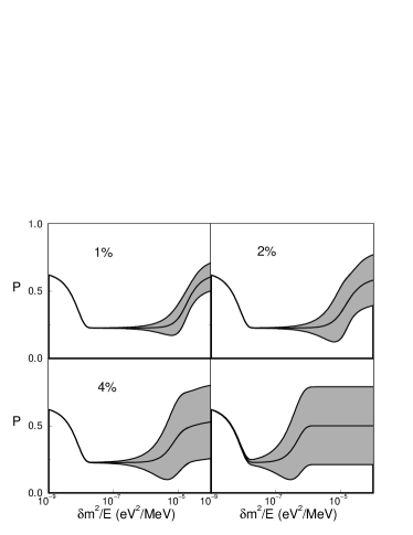
Figure 1: Mean electron neutrino survival probability plus minus $\sigma$ in the Sun with fluctuations. The average electron density is given by the Standard Solar Model of Bahcall and collaborators Bahcall et al. (2001) and $\tan^{2}2\theta=0.3$. The amount of the fluctuation (the value of $\beta$ in Eq. (3)) used in calculating each panel is indicated. For completeness the effects of an unrealistic fluctuation of $\beta$ = 50 % are also shown.

Using the formalism sketched above, it is possible to calculate not only the mean survival probability, but also the variance, $\sigma$, of the fluctuations to get a feeling for the distribution of the survival probabilities Balantekin et al. (1996) as illustrated in Figure 1. One notes that for very large fluctuations complete flavor de-polarization should be achieved, i.e. the neutrino survival probability is 0.5, the same as the vacuum oscillation probability with two flavors for long distances. To illustrate this behavior results from the physically unrealistic case of $\beta$ = 50% fluctuations are shown as well in the Figure 1 (the lower right-hand panel). One observes that for large values of $\delta m^{2}$ the average survival probability is indeed $0.5$ with a spread between a survival probability of $0$ and $1$ ($0.5\pm 0.5$). Detailed investigations indicate that the effect of the fluctuations is largest when the neutrino propagation in their absence is adiabatic Loreti et al. (1995); Balantekin et al. (1996). Note that the fluctuation analysis presented here is for two active flavors. This is exact only in the limit $U_{e3}=0$ Balantekin and Fuller (1999) when the solar electron neutrinos mix with an appropriate linear combination of the $\nu_{\mu}$’s and $\nu_{\tau}$’s determined by the atmospheric neutrino measurements. When $U_{e3}\neq 0$ a full three-flavor analysis is needed except for very special circumstances. However, since global analysis indicates that $U_{e3}\sim 0$ Fogli et al. (hep-ph/0106247) two-neutrino analysis may be rather accurate in the absence of sterile neutrinos.

In these calculations the correlation length $\tau_{c}$ is taken to be very small, of the order of 10 km., to be consistent with the helioseismic observations of the sound speed Bahcall et al. (2001, 1997). In the opposite limit of very large correlation lengths are very interesting result is obtained Loreti et al. (1995), namely the averaged density matrix is given as an integral

$$\lim_{\tau_{c}\to\infty}\langle\hat{\rho}(r)\rangle={1\over{\sqrt{2\pi\beta^{2}}}}\int_{-\infty}^{\infty}dx\exp[{-x^{2}/(2\beta^{2})}]\hat{\rho}(r,x),$$ (6)

reminiscent of the channel-coupling problem in nuclear physics Balantekin and Takigawa (1998). Even though this limit is not appropriate to the solar fluctuations it may be applicable to a number of other astrophysical situations where neutrinos play a role. Similar conclusions were reached by other authors Burgess and Michaud (1997); Nunokawa et al. (1997); Bamert et al. (1998); Nunokawa et al. (1999); Sahu and Bannur (2000); Bykov et al. (1999); Valle (2000); Bykov et al. (2000); Reggiani et al. (2000); Pantaleone (1998); Torrente-Lujan (1998, 1999); Prakash et al. (astro-ph/0103095); Bell et al. (quant-ph/0008133). Recent reviews were given in Refs. Balantekin (1999); Valle (astro-ph/0104085).

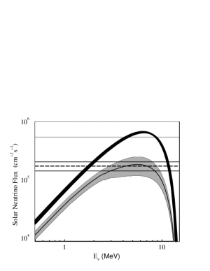
Figure 2: Solar Neutrino flux. The error range in the prediction of the Standard Solar Model is indicated by the black band. The spread of the electron neutrino flux due to $\beta$ = 1% fluctuations is indicated by the shaded area (the curve in the middle of the shaded area is the prediction for the average survival probability in the presence of the fluctuations with $\delta m^{2}=5\times 10^{-5}$ eV² and $\tan^{2}\theta=0.3$. The total energy-integrated solar electron neutrino flux observed in Sudbury Neutrino Observatory (the horizontal dashed line), the corresponding experimental error (two horizontal lines bordering the dashed line), as well as the spread of the total energy-integrated solar neutrino flux of all active flavors evaluated using the Sudbury Neutrino Observatory and SuperKamiokande data (three very closely spaced horizontal lines at the top of the figure) are also shown.

Recent Sudbury Neutrino Observatory measurements Ahmad et al. (nucl-ex/0106015) give the electron neutrino component of the solar ⁸B flux to be $1.75\pm 0.15\times 10^{6}$ cm^-2 s^-1. This result combined with the SuperKamiokande measurements Fukuda et al. (2001) give the flux of total active flavor component of the ⁸B neutrinos to be $5.44\pm 0.99\times 10^{6}$ cm^-2 s^-1 in good agreement with the Standard Solar Model prediction of $5.05\pm 0.80\times 10^{6}$ cm^-2 s^-1 Bahcall et al. (2001). (The theoretical error is large due to the large experimental uncertainty in the nuclear reactions forming ⁸B Adelberger et al. (1998)). These data are shown in Figure 2. The best fit to all the solar neutrino data is with $\delta m^{2}=5\times 10^{-5}$ eV² and $\tan^{2}\theta=0.3$. The mean solar electron neutrino flux in the presence of the fluctuations as well as its variance are also shown.

Figure 2 suggests that the Sudbury Neutrino Observatory charged-current measurements safely rule out solar electron density fluctuations of a few percent or more as such fluctuations would give rise to a much larger spread of the solar electron neutrino flux than that was observed (Strictly speaking the time-scale associated with the fluctuations should be incorporated in this argument; in the present discussion this time-scale is assumed to be much shorter than the total data-taking duration). A careful analysis of the time-structure of the future charged-current data at Sudbury Neutrino Observatory and the measurements of the ⁷Be-line at BOREXINO and KamLAND may be able to rule out fluctuations of much smaller amplitudes. Note that it is essential to take the variance into account in such an analysis; the mean survival probability in the presence of fluctuations is too close to the survival probability in the absence of fluctuations when $\beta=1$%.

The solar electron density fluctuations cause not only fluctuations in the solar $\nu_{e}$ flux, but, because of the unitarity, compensating fluctuations in the solar $\nu_{\mu}$ and $\nu_{\tau}$ flux. Consequently it is harder to perform such an analysis with $\nu_{\odot}$-electron elastic scattering since elastic scattering is sensitive to all flavors (albeit at a reduced rate for muon and tau neutrinos). A more detailed analysis of the possible signatures of fluctuations in the solar neutrino data will be published elsewhere Balantekin (2001).

Neutrino propagation in the presence of fluctuations was also investigated for the neutrino convection in a core-collapse supernova where the adiabaticity condition is well satisfied Loreti et al. (1995). In core-collapse supernovae neutrinos not only may play a very important role in shock re-heating Prakash et al. (astro-ph/0103095), but may also help solving a number of problems arising when such supernovae are considered as possible sites for r-process nucleosynthesis McLaughlin et al. (1999); Caldwell et al. (2000). Fluctuations are likely to be important in assessing the role of neutrinos in such phenomena.

References

- Ahmad et al. (nucl-ex/0106015) Ahmad, Q. R., et al. (nucl-ex/0106015).
- Fukuda et al. (2001) Fukuda, S., et al., Phys. Rev. Lett., 86, 5651–5655 (2001).
- Fogli et al. (hep-ph/0106247) Fogli, G. L., Lisi, E., Montanino, D., and Palazzo, A. (hep-ph/0106247).
- Bahcall et al. (hep-ph/0106258) Bahcall, J. N., Gonzalez-Garcia, M. C., and Pena-Garay, C. (hep-ph/0106258).
- Sawyer (1990) Sawyer, R. F., Phys. Rev., D42, 3908–3917 (1990).
- Schaefer and Koonin (1987) Schaefer, A., and Koonin, S. E., Phys. Lett., B185, 417–420 (1987).
- Krastev and Smirnov (1989) Krastev, P. I., and Smirnov, A. Y., Phys. Lett., B226, 341–346 (1989).
- Haxton and Zhang (1991) Haxton, W. C., and Zhang, W. M., Phys. Rev., D43, 2484–2494 (1991).
- Loreti and Balantekin (1994) Loreti, F. N., and Balantekin, A. B., Phys. Rev., D50, 4762–4770 (1994).
- Bahcall et al. (2001) Bahcall, J. N., Pinsonneault, M. H., and Basu, S., Astrophys. J., 555, 990–1012 (2001).
- Balantekin et al. (1996) Balantekin, A. B., Fetter, J. M., and Loreti, F. N., Phys. Rev., D54, 3941–3951 (1996).
- Loreti et al. (1995) Loreti, F. N., Qian, Y. Z., Fuller, G. M., and Balantekin, A. B., Phys. Rev., D52, 6664–6670 (1995).
- Balantekin and Fuller (1999) Balantekin, A. B., and Fuller, G. M., Phys. Lett., B471, 195–201 (1999).
- Bahcall et al. (1997) Bahcall, J. N., Basu, S., and Kumar, P., Astrophys. J., 485, L91–L94 (1997).
- Balantekin and Takigawa (1998) Balantekin, A. B., and Takigawa, N., Rev. Mod. Phys., 70, 77–100 (1998).
- Burgess and Michaud (1997) Burgess, C. P., and Michaud, D., Annals Phys., 256, 1–38 (1997).
- Nunokawa et al. (1997) Nunokawa, H., Semikoz, V. B., Smirnov, A. Y., and Valle, J. W. F., Nucl. Phys., B501, 17–40 (1997).
- Bamert et al. (1998) Bamert, P., Burgess, C. P., and Michaud, D., Nucl. Phys., B513, 319–342 (1998).
- Nunokawa et al. (1999) Nunokawa, H., Rossi, A., Semikoz, V., and Valle, J. W. F., Nucl. Phys. Proc. Suppl., 70, 345–347 (1999).
- Sahu and Bannur (2000) Sahu, S., and Bannur, V. M., Phys. Rev., D61, 023003 (2000).
- Bykov et al. (1999) Bykov, A. A., Popov, V. Y., Rez, A. I., Semikoz, V. B., and Sokoloff, D. D., Phys. Rev., D59, 063001 (1999).
- Valle (2000) Valle, J. W. F., Phys. Atom. Nucl., 63, 921–933 (2000).
- Bykov et al. (2000) Bykov, A. A., Gonzalez-Garcia, M. C., Pena-Garay, C., Popov, V. Y., and Semikoz, V. B. (2000).
- Reggiani et al. (2000) Reggiani, N., Guzzo, M. M., Colonia, J. H., and de Holanda, P. C., Braz. J. Phys., 30, 594–601 (2000).
- Pantaleone (1998) Pantaleone, J., Phys. Rev., D58, 073002 (1998).
- Torrente-Lujan (1998) Torrente-Lujan, E., Phys. Lett., B441, 305–312 (1998).
- Torrente-Lujan (1999) Torrente-Lujan, E., Phys. Rev., D59, 073001 (1999).
- Prakash et al. (astro-ph/0103095) Prakash, M., Lattimer, J. M., Sawyer, R. F., and Volkas, R. R. (astro-ph/0103095).
- Bell et al. (quant-ph/0008133) Bell, N. F., Sawyer, R. F., and Volkas, R. R. (quant-ph/0008133).
- Balantekin (1999) Balantekin, A. B., Phys. Rept., 315, 123–135 (1999).
- Valle (astro-ph/0104085) Valle, J. W. F. (astro-ph/0104085).
- Adelberger et al. (1998) Adelberger, E. G., et al., Rev. Mod. Phys., 70, 1265–1292 (1998).
- Balantekin (2001) Balantekin, A. B., to be published (2001).
- McLaughlin et al. (1999) McLaughlin, G. C., Fetter, J. M., Balantekin, A. B., and Fuller, G. M., Phys. Rev., C59, 2873–2887 (1999).
- Caldwell et al. (2000) Caldwell, D. O., Fuller, G. M., and Qian, Y.-Z., Phys. Rev., D61, 123005 (2000).