Determination of
Parton Distribution Functions in Nuclei

Abstract

Nuclear parton distribution functions are obtained by a $\chi^{2}$ analysis of lepton deep inelastic experimental data. It is possible to determine valence-quark distributions at medium $x$ and antiquark distributions at small $x$; however, the distributions in other $x$ regions and gluon distributions cannot be fixed. We need a variety of experimental data and also further analysis refinements.

1 Introduction

Nuclear parton distributions are used inevitably for calculating high-energy nuclear cross sections; however, precise distributions are not obtained yet. On the other hand, heavy-ion reactions have been investigated for finding a quark-gluon plasma signature. Because it should be found in any unusual cross section which cannot be explained by the present hadron physics framework, the parton distributions have to be known very precisely. Although there are many studies on quark-gluon plasma signatures, it is unfortunate that the same amount of efforts are not made for the initial condition, namely the parton distributions. In fact, many researchers just use the parton distributions in the “nucleon” instead of those in nuclei. It is known that nuclear distributions are modified from those in the nucleon, and the modification could be of the order of 20%. However, little information is available for nuclear gluon distributions, which play a crucial role for the $J/\psi$ production.

The nuclear parton distributions were investigated, for example, in Ref. 1, and the first $\chi^{2}$ analysis was reported in Ref. 2. However, it should be noted that the $\chi^{2}$ analysis is still at the preliminary stage in comparison with many solid investigations on the distributions in the nucleon. There are two major issues. First, there are not many available data for nuclei. In particular, the data come mainly from deep inelastic electron or muon scattering. Second, the technique of nuclear $\chi^{2}$ analysis is not established. The studies in Ref. 2 tried to set up a $\chi^{2}$ analysis method for the nuclear distributions.

In this paper, the optimum distributions obtained in Ref. 2 are explained. The analysis method is discussed in Sec. 2. Results are shown in Sec. 3, and a parton distribution library is explained in Sec. 4. Our studies are summarized in Sec. 5.

2 Analysis method

The nuclear parton distributions are defined at a fixed $Q^{2}$, which is taken 1 GeV² ($\equiv Q_{0}^{2}$). This $Q^{2}$ point is selected so that many experimental data become available and yet perturbative QCD is expected to be applied. Then, the nuclear distributions are defined by $x$ dependent functions multiplied by the distributions in the nucleon. It is analogous to polarized distributions. In the leading order (LO), the polarized distributions are restricted by the positivity condition. Namely, they should be smaller than the unpolarized ones. The positivity condition is easily handled if the polarized distributions are defined from the unpolarized.[3] In a similar way, it is technically easier to parametrize the modification part instead of the nuclear distributions themselves, because the nuclear modification is typically smaller than 20%. The nuclear parton distributions are then given as

$$f_{i}^{A}(x,Q_{0}^{2})=w_{i}(x,A,Z)\,f_{i}(x,Q_{0}^{2}),$$ (1)

where $f_{i}(x,Q_{0}^{2})$ is the $i$-type distribution in the nucleon, and $w_{i}(x,A,Z)$ is a weight function. As the distribution types, $i$=$u_{v}$, $d_{v}$, $\bar{q}$, and $g$ are taken. The distributions in the nucleon are taken from the MRST-LO parametrization.[4] The nuclear modification part $w_{i}(x,A,Z)$ is parametrized as

$$w_{i}(x,A,Z)=1+\left(1-\frac{1}{A^{1/3}}\right)\frac{a_{i}(A,Z)+b_{i}x+c_{i}x^{2}+d_{i}x^{3}}{(1-x)^{\beta_{i}}},$$ (2)

in terms of the parameters $a_{i}$, $b_{i}$, $c_{i}$, $d_{i}$, and $\beta_{i}$. At this stage, a simple $A$ dependent form ($\sim A^{1/3}$) is assumed [5] in order to avoid complexity. The function $1/(1-x)^{\beta_{i}}$ is introduced so as to reproduce the Fermi motion part at large $x$. The rest of the $x$ dependence is assumed in the cubic functional form, so that this $\chi^{2}$ analysis is called a “cubic” type. We also tried another simpler one, a “quadratic” type, without the $d_{i}x^{3}$ term in Eq. (2). There are three constraints for the parameters: the conditions for nuclear charge, baryon number, and momentum. Therefore, three parameters can be fixed.

Experimental data are taken from those in electron or muon deep inelastic scattering (DIS). The analysis with other data is in progress. There are also neutrino-nucleus data. However, it is difficult to address ourselves to the nuclear modification because there is no accurate data for the neutrino-deuteron scattering. The situation will change if a neutrino factory is materialized.[6]

The data are taken at various $Q^{2}$ points. The initial parton distributions are evolved to the experimental $Q^{2}$ points so as to calculate $\chi^{2}$:

$$\chi^{2}=\sum_{j}\frac{(R_{F_{2},j}^{A,data}-R_{F_{2},j}^{A,theo})^{2}}{(\sigma_{j}^{data})^{2}},$$ (3)

where $R_{F_{2}}^{A}(x,Q^{2})=F_{2}^{A}(x,Q^{2})/F_{2}^{D}(x,Q^{2})$. The analysis is done in the leading order of $\alpha_{s}$, so that the structure function $F_{2}^{A}$ is given by

$$F_{2}^{A}(x,Q^{2})=\sum_{q}e_{q}^{2}x[q^{A}(x,Q^{2})+\bar{q}^{A}(x,Q^{2})],$$ (4)

where $e_{q}$ is the quark charge, and $q^{A}$ ($\bar{q}^{A}$) is the quark (antiquark) distribution in the nucleus $A$. The data exist for various nuclei, which are assumed as ⁴He, ⁷Li, ⁹Be, ¹²C, ¹⁴N, ²⁷Al, ⁴⁰Ca, ⁵⁶Fe, ⁶³Cu, ¹⁰⁷Ag, ¹¹⁸Sn, ¹³¹Xe, ¹⁹⁷Au, and ²⁰⁸Pb in the theoretical analysis. The $Q^{2}$ evolution is calculated by the ordinary leading-order DGLAP equations.

3 Results

Table 1: $\chi^{2}$ contributions.

nucleus	# of data	$\chi^{2}$ (quad.)	$\chi^{2}$ (cubic)
He	35	55.6	54.5
Li	17	45.6	49.2
Be	17	39.7	38.4
C	43	97.8	88.2
N	9	10.5	10.4
Al	35	38.8	41.4
Ca	33	72.3	69.7
Fe	57	115.7	92.7
Cu	19	13.7	13.6
Ag	7	12.7	11.5
Sn	8	14.8	17.7
Xe	5	3.2	2.4
Au	19	55.5	49.2
Pb	5	7.9	7.6
total	309	583.7	546.6

The $\chi^{2}$ analysis was done with the help of the CERN Minuit subroutine. The detailed descriptions of the analysis should be found in Ref. 2. The obtained $\chi^{2}$ values are listed in Table 1. The table indicates that the fit is not excellent in lithium, carbon, calcium, iron, and gold. In comparison with the quadratic analysis, the fit becomes better notably for carbon, iron, and gold in the cubic type; however, by sacrificing $\chi^{2}$ values of some other nuclei. The number of the data is 309, so that $\chi^{2}$ per degrees of freedom is given by $\chi_{min}^{2}/d.o.f.$=1.93 (quadratic) or 1.82 (cubic). Because they are certainly much larger than one, they may not seem to be excellent fits. However, it is mainly due to the scattered experimental data.

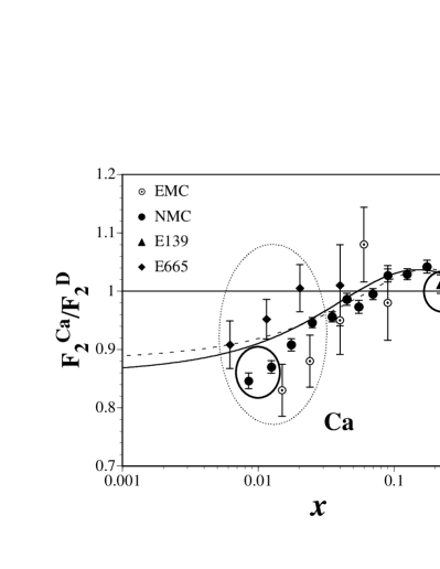
Figure 1: Comparison with calcium data.

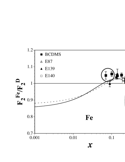
Figure 2: Comparison with iron data.

In order to specify the origin of the large $\chi^{2}$ contributions, we show our fitting results in comparison with the data in Figs. 2 and 2, where the solid circles indicate the major source of the $\chi^{2}$ contributions and the dotted ones indicate other sources. Our fitting results are shown by the dashed and solid curves for the quadratic and cubic analyses, respectively, and they are calculated at $Q^{2}$=5 GeV². Although they cannot be directly compared with the data due to the $Q^{2}$ difference, the figures suggest that the fits should be well done. Both results are almost the same except for the small $x$ region, where the data do not exist. It is obvious from these figures that the data are scattered and some of them have very small errors, which contribute mostly to the total $\chi^{2}$. Even if an excellent $\chi^{2}$ analysis method is developed in future by introducing complicated $A$ and $x$ dependence, it is inevitable to obtain $\chi^{2}/d.o.f.>1$ in the present experimental situation.

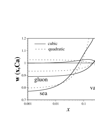
Figure 3: Weight functions.

Next, obtained weight functions are shown for the calcium nucleus in Fig. 3, where the dashed and solid curves indicate the results for the quadratic and cubic analysis, respectively, at $Q^{2}$=1 GeV². As expected, the valence-quark distributions explain the EMC effect at medium $x$ and they have Fermi-motion-type increase at large $x$. However, the small $x$ behavior is far from obvious. It could show either antishadowing or shadowing. A precise determination of the valence distributions, especially at small $x$, should be done by a future neutrino factory.[6]

The antiquark distributions at small $x$ are restricted by the $F_{2}^{A}$ shadowing, so that they could be fixed in this $x$ region. However, they cannot be determined at medium and large $x$. If the Drell-Yan data are added to the analysis, we expect to have more restriction on the antiquark distributions at $x\sim 0.1$.

On the other hand, the gluon distribution cannot be determined well in the present analysis. The inclusive DIS data are not sensitive to the gluon distributions, especially in the LO analysis. At this stage, the gluon distributions seem to show shadowing at small $x$, and they increase at large $x$ because of the momentum conservation. In future, we should consider to include the data which could restrict the gluon distributions.

4 Parton distribution codes

From the $\chi^{2}$ analysis, the parton distributions are obtained for nuclei from the deuteron to a large nucleus with $A\sim 208$. Because variations are small from $A=208$ to nuclear matter, we expect the distributions could be extrapolated into larger $A$ $(>208)$. We set up the initial distributions at $Q^{2}$=1 GeV². However, we made it possible to calculate the distributions at any $Q^{2}$ by our computer codes, because the $Q^{2}$ evolution may be tedious for some users. The codes can be obtained from our web site.[7] There are two possibilities of using our results for the parton distributions in a user’s project. One is to use the analytical expressions for the weight functions, and another is to use the computer codes. Strictly speaking, the obtained distributions are valid for the analyzed nuclei, helium, lithium, $\cdot\cdot\cdot$, and lead. However, the $A$ dependence is reproduced well even by the simple $1/A^{1/3}$ form, so that our studies are expected to be used also for other nuclei except for unstable ones with large neutron excess.

Analytical expressions

For those who have own $Q^{2}$ evolution codes, we wrote the analytical expressions of the weight functions in Appendix of Ref. 2. They should be multiplied by the MRST-LO distributions in the nucleon so as to obtain the nuclear distributions at $Q^{2}$=1 GeV². Then, they should be evolved to a $Q^{2}$ point in a user’s project. Because the parton distributions in the nucleon are similar among various groups, the results are not expected to change significantly even if other parametrization is used instead of the MRST-LO.

Computer codes

For those who are not familiar with the $Q^{2}$ evolution, we supply our own codes for calculating the nuclear parton distributions at any $Q^{2}$. Grid data are prepared for the distributions with the variables $x$ and $Q^{2}$, and they are interpolated. If one wishes to run the actual evolution, we also supply a $Q^{2}$ evolution package. The detailed instructions should be found in the distributed file, saga01.tar.gz.[7]

5 Summary

We have obtained optimum parton distributions in nuclei by the $\chi^{2}$ analysis of DIS experimental data. At this stage, our studies are intended to set up a tool for the nuclear $\chi^{2}$ analysis, which had not been done at all until recently. It is still far from completion in the sense that analysis refinements are needed and a variety of experimental data should be included in the analysis. We continue to work on this project for obtaining reliable parton distributions in nuclei.

References

- [1] K. J. Eskola, V. J. Kolhinen, and P. V. Ruuskanen, Nucl. Phys. B535, 351 (1998).
- [2] M. Hirai, S. Kumano, and M. Miyama, Phys. Rev. D64, 034003 (2001).
- [3] Y. Goto et. al. (AAC), Phys. Rev. D62, 034017 (2000). The AAC library is available at http://spin.riken.bnl.gov/aac.
- [4] A. D. Martin, R. G. Roberts, W. J. Stirling, and R. S. Thorne, Eur. Phys. J. C4, 463 (1998).
- [5] I. Sick and D. Day, Phys. Lett. B274, 16 (1992).
- [6] S. Kumano, hep-ph/0109046; http://hs.phys.saga-u.ac.jp/talk01.html and talk00.html for talks on a neutrino factory.
-
[7]