ZU-TH 8/01

LMU-xx-/01

DESY 01-128

Complex flavour couplings in supersymmetry and unexpected $\mathbf{C}P$-violation in the decay $B\to\phi K$

E. Lunghi***E-mail: lunghi@mail.desy.de and D. Wylerโ€ โ€ โ€ permanent address: Theoretische Physik, Universitรคt Zรผrich Winterthurerstrasse 190, CH-8057, Zรผrich. E-mail: wyler@physik.unizh.ch
Deutsches Elektronen Synchrotron, DESY,

Notkestrasse 85, D-22607, Hamburg, Germany

Abstract

Complex flavour couplings (off-diagonal mass terms) in the squark sector of supersymmetric theories may drastically alter both the rate and the $CP$-violating asymmetry of certain $B$-meson decays. We consider the effects of couplings that induce bโ†’sโ†’๐‘๐‘ b\to s transitions and lead to final state with strangeness one. We investigate the bounds that must be satisfied by the new terms and explore the possible implications on direct and mixing induced asymmetries in the charged and neutral $B\to J/\Psi K$ and $B\to\phi K$ decays.

1 Introduction

Certain decays of $B$-mesons are expected to shed light on the mechanism of $CP$ violation and, more generally, on new physics. Indeed, the first surprising results on the $CP$-asymmetry $a_{\psi K}$ in the decay $B\to J/\Psi K$ raised the hope for a first new physics signal. Meanwhile, the value of the measured asymmetry has changed considerably and the present world averageย [1]

$$a_{\psi K}^{WA}=0.79\pm 0.12$$ (1)

almost coincides with the standard model expectationย [2]

$$a_{\psi K}^{SM}\simeq 0.70\pm 0.10\;.$$ (2)

Although this came as a disappointment, it reinforced the view that one should be prepared, both on the theoretical and the experimental side, for unexpected observations. In fact, the small error of the above world average and the improvements that are expected during the next years will allow to detect even small deviations from the standard model predictions.

There are of course many new physics scenarios. On the one hand, it is possible to describe their signatures in very general terms (for recent expositions, see e.g. Refs.ย [3, 4, 5]). On the other hand, one can propose a specific new physics model and investigate its consequences. The latter approach was the topic of a huge body of work. For what concerns supersymmetric models, emphasis was given recently to the so-called minimal flavour violating models (MFV)ย [6] and their possible variantsย [7].

In virtually all new physics models, new non-standard fields are introduced and, therefore, new complex (i.e. with $CP$-violating phases) couplings appear. This is well known in supersymmetry to which we turn for definiteness. In supersymmetric models there are several classes of phases. Those in the $\mu$ and flavour diagonal $A$ terms do not contribute to flavour changing processes but are strongly bound by the electric dipole moment of the neutron and other particlesย [8]. The phases of the Yukawa couplings are the same as in the standard model. If these are the only phases and flavour changing couplings of a model, the latter belongs to the class of MFV supersymmetric models that exhibit many analogies to the standard modelย [6]. Therefore, the most interesting phases are those in the squark and slepton mass matrices. Their flavour diagonal elements are either real by definition (in the $LL$ and $RR$ sectors) or small (in the $LR$ and $RL$ ones) as pointed out before (restrictions from electric dipole moments). Therefore the flavour changing elements (i.e. $(m^{2})_{23}^{u,d}$ and $(m^{2})_{13}^{u,d}$, in the sectors $LL$, $RL$, etc.) are the most interesting ones and we will focus on their effects. They contribute mainly through loop diagrams with internal gluinos and charginos. Since we are interested in contributions to Wilson coefficients that are already quite large in the SMย โ€กโ€กโ€กContributions to the small electroweak penguin coefficients are usually negligible because they do not appreciably change the standard model predictions.(i.e. the coefficients of the QCD penguin and chromo-magnetic dipole moment operators), we will only discuss gluino loops; in fact, they tend to dominate over the corresponding chargino ones.

Clearly this is not the first analysis of such SUSY diagrams. Their impact on flavour physics is known since a long timeย [9], and there are numerous recent investigations. To clarify the new aspects provided in this paper, we review briefly some of the most recent efforts.

In Ref.ย [10] a first comprehensive analysis of the gluino exchanges was given. The systematics of the perturbative expansion was investigated in Ref.ย [11], which also included an analysis of the mass insertion approximation: the latter was found to be sufficient in many cases and we will use it again in this study. In Ref.ย [12] the bounds from the rare decay bโ†’sโ€‹ฮณโ†’๐‘๐‘ ๐›พb\to s\gamma were derived; however, the various couplings were assumed to be real. In Ref.ย [13], the influence on the electromagnetic penguins (isospin violating terms) and the consequences on $B\to K\pi$ decays were studied; particular focus was given to the determination of the $CKM$ angle $\gamma$. In Ref.ย [3] effects of new terms on direct $CP$-violating asymmetries in charged decays were given, but the possible values of the new coefficients were not investigated. In Ref.ย [5] a completely general parameterization of new physics effects in the decays $B\to\phi K$ and $B\to J/\Psi K$ was given; however, no particular model was explicitely studied. In Ref.ย [14], the case of left-right symmetric models were investigated and it was found that, in these models, sizeable deviations from the relation $a_{\psi K}=a_{\phi K}$ are possible.

In this paper, we consider the complex $(2,3)$ entries in the down squark mass matrix and work out their consequences for the time dependent $CP$ asymmetries in the decays $B\to\phi K$ and $B\to J/\Psi K$. In the standard model, these asymmetries are equal and are a measure of the phase of the $B_{d}$-$\bar{B}_{d}$ mixing amplitude (which in the SM is $2\beta$). The complex couplings that we consider leave the $B_{d}$-$\bar{B}_{d}$ mixing phase unchanged but have a significant impact on the amplitudes of the decays. The $B\to J/\Psi K$ amplitude is dominated by SM tree level contributions and, consequently, the $CP$-violating asymmetry is hardly modified; on the other hand, there is room for such an effect in the transition $B\to\phi K$. This decay is easily accessible at the $B$-factory experimentsย [15] and an investigation of the related $CP$ asymmetries is clearly worthwhile. In the analysis we will concentrate on this decay.

This note is organized as follows. In Sec.ย 2 we review the effective Hamiltonian for bโ†’sโ€‹sยฏโ€‹sโ†’๐‘๐‘ ยฏ๐‘ ๐‘ b\to s\bar{s}s transitions in generic extensions of the standard model and give the explicit expressions of the various $CP$ asymmetries. We also discuss the observables โ„ฌโ€‹(Bโ†’Xsโ€‹ฮณ)โ„ฌโ†’๐ตsubscript๐‘‹๐‘ ๐›พ{\cal B}(B\to X_{s}\gamma) and ฮ”โ€‹MBsฮ”subscript๐‘€subscript๐ต๐‘ \Delta M_{B_{s}} which are related to the bโ†’sโ†’๐‘๐‘ b\to s transition and provide interesting additional pieces of information. In Sec.ย 3 we present the SUSY model that we consider and the explicit contributions to the Wilson coefficients. The numerical analysis is presented in Sec.ย 4. The impact of the complex SUSY parameters on the branching ratio and $CP$ asymmetry of Bโ†’Xsโ€‹ฮณโ†’๐ตsubscript๐‘‹๐‘ ๐›พB\to X_{s}\gamma is explored and we analyze the correlation between the mixing-induced (and direct) $CP$ asymmetries in $B\to\phi K$ and the Bssubscript๐ต๐‘ B_{s}-Bยฏssubscriptยฏ๐ต๐‘ {\bar{B}}_{s} mass difference. A brief summary of our results and some comments are found in Sec.ย 5.

2 Effective Hamiltonian

The effective Hamiltonian for bโ†’sโ†’๐‘๐‘ b\to s transitions can be written as

โ„‹eโ€‹fโ€‹f=GF2โ€‹Vtโ€‹bโ€‹Vtโ€‹sโˆ—โ€‹[โˆ‘i=110Ciโ€‹(ฮผ)โ€‹๐’ชi+C7โ€‹ฮณโ€‹๐’ช7โ€‹ฮณ+C8โ€‹gโ€‹๐’ช8โ€‹g]subscriptโ„‹๐‘’๐‘“๐‘“subscript๐บ๐น2subscript๐‘‰๐‘ก๐‘superscriptsubscript๐‘‰๐‘ก๐‘ delimited-[]superscriptsubscript๐‘–110subscript๐ถ๐‘–๐œ‡subscript๐’ช๐‘–subscript๐ถ7๐›พsubscript๐’ช7๐›พsubscript๐ถ8๐‘”subscript๐’ช8๐‘”{\cal{H}}_{eff}={G_{F}\over\sqrt{2}}V_{tb}V_{ts}^{*}\left[\sum_{i=1}^{10}C_{i}(\mu){\cal O}_{i}+C_{7\gamma}{\cal O}_{7\gamma}+C_{8g}{\cal O}_{8g}\right] (3)

where ($e_{u,c}=2/3$ and ed,s,b=โˆ’1/3subscript๐‘’๐‘‘๐‘ ๐‘13e_{d,s,b}=-1/3)

$\displaystyle{\cal O}_{1}$ $\displaystyle=$ (cยฏฮฑโ€‹bฮฒ)Vโˆ’Aโ€‹(sยฏฮฒโ€‹cฮฑ)Vโˆ’Asubscriptsubscriptยฏ๐‘๐›ผsubscript๐‘๐›ฝ๐‘‰๐ดsubscriptsubscriptยฏ๐‘ ๐›ฝsubscript๐‘๐›ผ๐‘‰๐ด\displaystyle(\bar{c}_{\alpha}b_{\beta})_{V-A}(\bar{s}_{\beta}c_{\alpha})_{V-A} (4)
$\displaystyle{\cal O}_{2}$ $\displaystyle=$ (cยฏโ€‹b)Vโˆ’Aโ€‹(sยฏโ€‹c)Vโˆ’Asubscriptยฏ๐‘๐‘๐‘‰๐ดsubscriptยฏ๐‘ ๐‘๐‘‰๐ด\displaystyle(\bar{c}b)_{V-A}(\bar{s}c)_{V-A} (5)
$\displaystyle{\cal O}_{3}$ $\displaystyle=$ (sยฏโ€‹b)Vโˆ’Aโ€‹โˆ‘q=u,d,s,c,b(qยฏโ€‹q)Vโˆ’Asubscriptยฏ๐‘ ๐‘๐‘‰๐ดsubscript๐‘ž๐‘ข๐‘‘๐‘ ๐‘๐‘subscriptยฏ๐‘ž๐‘ž๐‘‰๐ด\displaystyle(\bar{s}b)_{V-A}\sum_{q=u,d,s,c,b}(\bar{q}q)_{V-A} (6)
$\displaystyle{\cal O}_{4}$ $\displaystyle=$ (sยฏฮฑโ€‹bฮฒ)Vโˆ’Aโ€‹โˆ‘q=u,d,s,c,b(qยฏฮฒโ€‹qฮฑ)Vโˆ’Asubscriptsubscriptยฏ๐‘ ๐›ผsubscript๐‘๐›ฝ๐‘‰๐ดsubscript๐‘ž๐‘ข๐‘‘๐‘ ๐‘๐‘subscriptsubscriptยฏ๐‘ž๐›ฝsubscript๐‘ž๐›ผ๐‘‰๐ด\displaystyle(\bar{s}_{\alpha}b_{\beta})_{V-A}\sum_{q=u,d,s,c,b}(\bar{q}_{\beta}q_{\alpha})_{V-A} (7)
$\displaystyle{\cal O}_{5}$ $\displaystyle=$ (sยฏโ€‹b)Vโˆ’Aโ€‹โˆ‘q=u,d,s,c,b(qยฏโ€‹q)V+Asubscriptยฏ๐‘ ๐‘๐‘‰๐ดsubscript๐‘ž๐‘ข๐‘‘๐‘ ๐‘๐‘subscriptยฏ๐‘ž๐‘ž๐‘‰๐ด\displaystyle(\bar{s}b)_{V-A}\sum_{q=u,d,s,c,b}(\bar{q}q)_{V+A} (8)
$\displaystyle{\cal O}_{6}$ $\displaystyle=$ (sยฏฮฑโ€‹bฮฒ)Vโˆ’Aโ€‹โˆ‘q=u,d,s,c,b(qยฏฮฒโ€‹qฮฑ)V+Asubscriptsubscriptยฏ๐‘ ๐›ผsubscript๐‘๐›ฝ๐‘‰๐ดsubscript๐‘ž๐‘ข๐‘‘๐‘ ๐‘๐‘subscriptsubscriptยฏ๐‘ž๐›ฝsubscript๐‘ž๐›ผ๐‘‰๐ด\displaystyle(\bar{s}_{\alpha}b_{\beta})_{V-A}\sum_{q=u,d,s,c,b}(\bar{q}_{\beta}q_{\alpha})_{V+A} (9)
$\displaystyle{\cal O}_{7}$ $\displaystyle=$ 32โ€‹(sยฏโ€‹b)Vโˆ’Aโ€‹โˆ‘q=u,d,s,c,beqโ€‹(qยฏโ€‹q)Vโˆ’A32subscriptยฏ๐‘ ๐‘๐‘‰๐ดsubscript๐‘ž๐‘ข๐‘‘๐‘ ๐‘๐‘subscript๐‘’๐‘žsubscriptยฏ๐‘ž๐‘ž๐‘‰๐ด\displaystyle{3\over 2}(\bar{s}b)_{V-A}\sum_{q=u,d,s,c,b}e_{q}(\bar{q}q)_{V-A} (10)
$\displaystyle{\cal O}_{8}$ $\displaystyle=$ 32โ€‹(sยฏฮฑโ€‹bฮฒ)Vโˆ’Aโ€‹โˆ‘q=u,d,s,c,beqโ€‹(qยฏฮฒโ€‹qฮฑ)Vโˆ’A32subscriptsubscriptยฏ๐‘ ๐›ผsubscript๐‘๐›ฝ๐‘‰๐ดsubscript๐‘ž๐‘ข๐‘‘๐‘ ๐‘๐‘subscript๐‘’๐‘žsubscriptsubscriptยฏ๐‘ž๐›ฝsubscript๐‘ž๐›ผ๐‘‰๐ด\displaystyle{3\over 2}(\bar{s}_{\alpha}b_{\beta})_{V-A}\sum_{q=u,d,s,c,b}e_{q}(\bar{q}_{\beta}q_{\alpha})_{V-A} (11)
$\displaystyle{\cal O}_{9}$ $\displaystyle=$ 32โ€‹(sยฏโ€‹b)Vโˆ’Aโ€‹โˆ‘q=u,d,s,c,beqโ€‹(qยฏโ€‹q)V+A32subscriptยฏ๐‘ ๐‘๐‘‰๐ดsubscript๐‘ž๐‘ข๐‘‘๐‘ ๐‘๐‘subscript๐‘’๐‘žsubscriptยฏ๐‘ž๐‘ž๐‘‰๐ด\displaystyle{3\over 2}(\bar{s}b)_{V-A}\sum_{q=u,d,s,c,b}e_{q}(\bar{q}q)_{V+A} (12)
$\displaystyle{\cal O}_{10}$ $\displaystyle=$ 32โ€‹(sยฏฮฑโ€‹bฮฒ)Vโˆ’Aโ€‹โˆ‘q=u,d,s,c,beqโ€‹(qยฏฮฒโ€‹qฮฑ)V+A32subscriptsubscriptยฏ๐‘ ๐›ผsubscript๐‘๐›ฝ๐‘‰๐ดsubscript๐‘ž๐‘ข๐‘‘๐‘ ๐‘๐‘subscript๐‘’๐‘žsubscriptsubscriptยฏ๐‘ž๐›ฝsubscript๐‘ž๐›ผ๐‘‰๐ด\displaystyle{3\over 2}(\bar{s}_{\alpha}b_{\beta})_{V-A}\sum_{q=u,d,s,c,b}e_{q}(\bar{q}_{\beta}q_{\alpha})_{V+A} (13)
$\displaystyle{\cal O}_{7\gamma}$ $\displaystyle=$ e4โ€‹ฯ€2โ€‹mbโ€‹sยฏLโ€‹ฯƒฮผโ€‹ฮฝโ€‹bRโ€‹Fฮผโ€‹ฮฝ๐‘’4superscript๐œ‹2subscript๐‘š๐‘subscriptยฏ๐‘ ๐ฟsuperscript๐œŽ๐œ‡๐œˆsubscript๐‘๐‘…subscript๐น๐œ‡๐œˆ\displaystyle{e\over 4\pi^{2}}m_{b}\bar{s}_{L}\sigma^{\mu\nu}b_{R}F_{\mu\nu} (14)
$\displaystyle{\cal O}_{8g}$ $\displaystyle=$ gs4โ€‹ฯ€2โ€‹mbโ€‹sยฏLโ€‹ฯƒฮผโ€‹ฮฝโ€‹Taโ€‹bRโ€‹Gฮผโ€‹ฮฝa.subscript๐‘”๐‘ 4superscript๐œ‹2subscript๐‘š๐‘subscriptยฏ๐‘ ๐ฟsuperscript๐œŽ๐œ‡๐œˆsuperscript๐‘‡๐‘Žsubscript๐‘๐‘…superscriptsubscript๐บ๐œ‡๐œˆ๐‘Ž\displaystyle{g_{s}\over 4\pi^{2}}m_{b}\bar{s}_{L}\sigma^{\mu\nu}T^{a}b_{R}G_{\mu\nu}^{a}\;. (15)

In Eq.ย (3), we did not write the operators ${\cal O}_{1,2}^{u}$ obtained by the replacements $c\to u$ in ${\cal O}_{1,2}$, and the semileptonic currentโ€“current operators which induce the transitions bโ†’sโ€‹โ„“+โ€‹โ„“โˆ’โ†’๐‘๐‘ superscriptโ„“superscriptโ„“b\to s\ell^{+}\ell^{-}. The effective Hamiltonian for $b\to d$ transitions can be obtained via the substitution sโ†’dโ†’๐‘ ๐‘‘s\to d. Also, operators with different helicity structures are not explicitely written and can be obtained from the above operator basis via the replacement $L\leftrightarrow R$ย [11]. We will comment on their impact on the numerical analysis in sectionย 4.

The SM values of the Wilson coefficients $C_{1-10}(m_{b})$ and $C_{7\gamma,8g}(m_{b})$ are given in tableย 1; the opposite chirality operators do not get standard model contributions if the light masses are neglected.

$C_{1}$ -0.171 $C_{7}$ -0.00001
$C_{2}$ 1.070 $C_{8}$ 0.0005
$C_{3}$ 0.0114 $C_{9}$ -0.01
$C_{4}$ -0.0321 $C_{10}$ 0.0002
$C_{5}$ 0.00925 $C_{7\gamma}$ -0.313
$C_{6}$ -0.0383 $C_{8g}$ -0.188
Table 1: SM Wilson coefficients at the scale $m_{b}$.

We will use the following approximate formย ยงยงยงThis expression is based on naive factorization and is therefore not exact; but it correctly describes the way new physics enters. for the $B\to(J/\Psi,\phi)K$ amplitudesย [3]:

$\displaystyle{\cal A}^{\psi}$ $\displaystyle=$ โˆ’2โ€‹GFโ€‹fฯˆโ€‹F1Bโ†’Kโ€‹(mฯˆ2)โ€‹mฯˆโ€‹(ฯตฯˆโ‹…pB)โ€‹Vtโ€‹bโ€‹Vtโ€‹sโˆ—โ€‹[Cฯˆ+ฮฑs2โ€‹ฯ€โ€‹mB2mฯˆ2โ€‹C8โ€‹gโ€‹r8โ€‹S~ฯˆโ€‹K],2subscript๐บ๐นsubscript๐‘“๐œ“superscriptsubscript๐น1โ†’๐ต๐พsubscriptsuperscript๐‘š2๐œ“subscript๐‘š๐œ“โ‹…subscriptitalic-ฯต๐œ“subscript๐‘๐ตsubscript๐‘‰๐‘ก๐‘superscriptsubscript๐‘‰๐‘ก๐‘ delimited-[]subscript๐ถ๐œ“subscript๐›ผ๐‘ 2๐œ‹superscriptsubscript๐‘š๐ต2superscriptsubscript๐‘š๐œ“2subscript๐ถ8๐‘”subscript๐‘Ÿ8subscript~๐‘†๐œ“๐พ\displaystyle-\sqrt{2}G_{F}\;f_{\psi}\;F_{1}^{B\to K}(m^{2}_{\psi})\;m_{\psi}\;(\epsilon_{\psi}\cdot p_{B})\;V_{tb}V_{ts}^{*}\left[C_{\psi}+{\alpha_{s}\over 2\pi}{m_{B}^{2}\over m_{\psi}^{2}}C_{8g}r_{8}\tilde{S}_{\psi K}\right]\;, (16)
$\displaystyle{\cal A}^{\phi}$ $\displaystyle=$ โˆ’2โ€‹GFโ€‹fฯ•โ€‹F1Bโ†’Kโ€‹(mฯ•2)โ€‹mฯ•โ€‹(ฯตฯ•โ‹…pB)โ€‹Vtโ€‹bโ€‹Vtโ€‹sโˆ—โ€‹[Cฯ•+89โ€‹P+ฮฑs4โ€‹ฯ€โ€‹mb2q2โ€‹C8โ€‹gโ€‹S~ฯ•โ€‹K].2subscript๐บ๐นsubscript๐‘“italic-ฯ•superscriptsubscript๐น1โ†’๐ต๐พsubscriptsuperscript๐‘š2italic-ฯ•subscript๐‘šitalic-ฯ•โ‹…subscriptitalic-ฯตitalic-ฯ•subscript๐‘๐ตsubscript๐‘‰๐‘ก๐‘superscriptsubscript๐‘‰๐‘ก๐‘ delimited-[]subscript๐ถitalic-ฯ•89๐‘ƒsubscript๐›ผ๐‘ 4๐œ‹superscriptsubscript๐‘š๐‘2superscript๐‘ž2subscript๐ถ8๐‘”subscript~๐‘†italic-ฯ•๐พ\displaystyle-\sqrt{2}G_{F}\;f_{\phi}\;F_{1}^{B\to K}(m^{2}_{\phi})\;m_{\phi}\;(\epsilon_{\phi}\cdot p_{B})\;V_{tb}V_{ts}^{*}\left[C_{\phi}+{8\over 9}P+{\alpha_{s}\over 4\pi}{m_{b}^{2}\over q^{2}}C_{8g}\tilde{S}_{\phi K}\right]. (17)

Here, $f_{\psi(\phi)}$ is the decay constant of the $J/\Psi(\phi)$, $F_{1}^{B\to K}(q^{2})$ is the $B\to K$ penguin form factor, $\tilde{S}_{(\phi,\psi)K}\simeq-0.76$ is the ratio of the chromo-magnetic to penguin form factors for the $B\to(J/\Psi,\phi)K$ decay, $q^{2}\simeq m_{b}^{2}/2$, and $r_{8}\simeq 1/12$ is the ratio of colour octet and singlet matrix elements. $P$ is an Oโ€‹(ฮฑs)๐‘‚subscript๐›ผ๐‘ O(\alpha_{s}) contribution to the matrix elements of the QCD penguin operators, it is insensitive to new short distance physics, and it is originated by loop diagrams with an internal charm quark. Since the typical $q^{2}$ is above the charm production threshold, $P$ carries a strong phase and its numerical value is $-0.0132-i\;0.0145$ย [16]. Finally, the coefficients $C_{\psi,\phi}$ are

$\displaystyle C_{\psi}$ $\displaystyle=$ $\displaystyle C_{1}+C_{3}+C_{5}+{C_{2}+C_{4}+C_{6}\over 3}+2r_{8}(C_{2}+C_{4}+C_{6})$ (18)
$\displaystyle C_{\phi}$ $\displaystyle=$ $\displaystyle C_{3}+C_{4}+C_{5}+{C_{3}+C_{4}+C_{6}\over 3}-{1\over 2}\left(C_{7}+C_{9}+C_{10}+{C_{8}+C_{9}+C_{10}\over 3}\right)$ (19)

where all the $C_{i}$ are to be evaluated at the scale $m_{b}$.

New physics contribute to the above Wilson coefficients; the resulting new phases will show up in the direct and mixing induced $CP$ asymmetries. Before writing an explicit model for such contributions, we briefly discuss the renormalization group (RG) running of $C_{\psi,\phi}(\mu)$ from $\mu=O(M_{W})$ to $\mu=O(m_{b})$. The solution of the NLO RG equations reads:

$\displaystyle C_{\psi}(m_{b})$ $\displaystyle=$ $\displaystyle 0.3515\left(1+0.0018\;R_{3}-0.0014\;R_{4}+0.0020\;R_{5}+0.0053\;R_{6}\right)\;,$ (20)
$\displaystyle C_{\phi}(m_{b})$ $\displaystyle=$ $\displaystyle-0.0243\left(1-0.030\;R_{3}+0.085\;R_{4}-0.028\;R_{5}+0.044\;R_{6}\right)$ (21)

where $R_{i}\equiv C_{i}(M_{W})/C_{i}^{SM}(M_{W})$ and the other coefficients are fixed to their SM value. It follows that the impact of the QCD penguin matching conditions (the values of the Wilson coefficients at the scale $M_{W}$) on $C_{\psi}(m_{b})$ and $C_{\phi}(m_{b})$ is respectively of order $1\%$ and $10\%$. Thus, as it is well known, their effects on $C_{\psi}(m_{b})$ is totally negligible: the coefficients of the current-current operators totally dominate the amplitude even if their contribution is colour suppressed. Thus, the SM prediction of an extremely small direct $CP$ asymmetry in the $J/\Psi$ mode is unaltered by new physics contributions. On the other hand, new physics whose contributions are large enough to dominate the phases of $C_{3-6}(M_{W})$, may modify the overall phase of $C_{\phi}(m_{b})$ at the $10\%$ level. Taking into account that the $CP$ asymmetry depends on twice the phase of $C_{\phi}(m_{b})$, we see that in principle large ($O(0.2)$) deviations from the SM relation $a_{\psi K}=a_{\phi K}$ are possible. Moreover, the presence of a term proportional to $C_{8g}$ in Eq.ย (17) can have a strong impact if there are large new complex contributions to the chromo-magnetic dipole operator. In the standard model, this term is negligible.

Let us introduce the time-dependent $CP$ asymmetry in the decays $B_{d}^{0}/\overline{B_{d}^{0}}\to\phi K$, given by

$$a_{\phi K}(t)\equiv\frac{\Gamma(B_{d}^{0}(t)\to\phi K)-\Gamma(\overline{B_{d}^{0}}(t)\to\phi K)}{\Gamma(B_{d}^{0}(t)\to\phi K)+\Gamma(\overline{B_{d}^{0}}(t)\to\phi K)}={\cal A}_{\rm CP}^{\rm dir}\cos(\Delta M_{B_{d}}t)+{\cal A}_{\rm CP}^{\rm mix}\sin(\Delta M_{B_{d}}t)\;,$$ (22)

where $\Delta M_{B_{d}}$ is the is the $B_{d}$ -$\overline{B_{d}}$ mass difference and $B_{d}^{0}(t)\;(\overline{B_{d}^{0}}(t))$ is the state at time $t$ which started as a pure $B_{d}^{0}\;(\overline{B_{d}^{0}})$ at $t=0$. ${\cal A}_{\rm CP}^{\rm dir}$ and ${\cal A}_{\rm CP}^{\rm mix}$ are the direct and mixing-induced CP-asymmetries, respectively. Their explicit expressions are

$\displaystyle{\cal A}_{\rm CP}^{\rm dir}$ $\displaystyle=$ $\displaystyle{1-|\lambda_{\phi K}|^{2}\over 1+|\lambda_{\phi K}|^{2}}$ (23)
$\displaystyle{\cal A}_{\rm CP}^{\rm mix}$ $\displaystyle=$ $\displaystyle{2\hbox{Im}\lambda_{\phi K}\over 1+|\lambda_{\phi K}|^{2}}$ (24)

with

$$\lambda_{\phi K_{S}}=e^{2i(\beta+\theta_{d})}{\bar{A}\over A}\equiv e^{2i(\beta+\theta_{d}+\theta_{A})}\left|\bar{A}\over A\right|.$$ (25)

Here, $\beta$ is the inner angle of the unitarity triangle of the standard model, $\theta_{d}$ is a possible new physics contribution to the phase of the $B_{d}-\bar{B}_{d}$ oscillations, and $A$ ($\bar{A}$) are the amplitudes of the decay in question (and its $CP$ conjugate).

We turn next to the branching ratio and $CP$ asymmetry in the decay Bโ†’Xsโ€‹ฮณโ†’๐ตsubscript๐‘‹๐‘ ๐›พB\to X_{s}\gamma and to the Bssubscript๐ต๐‘ B_{s}-Bยฏssubscriptยฏ๐ต๐‘ \bar{B}_{s} mass difference. These observables are strongly affected by new physics in the FCNC bโ†’sโ†’๐‘๐‘ b\to s transition and therefore must be properly accounted for.

2.1 Bโ†’Xsโ€‹ฮณโ†’๐ตsubscript๐‘‹๐‘ ๐›พB\to X_{s}\gamma

The inclusive transition Bโ†’Xsโ€‹ฮณโ†’๐ตsubscript๐‘‹๐‘ ๐›พB\to X_{s}\gamma plays a major role in limiting possible new physics contributions to $B$ decays both through constraints on the branching ratio and on direct $CP$ asymmetry. The experimental information on the latter quantities isย [17]

โ„ฌโ€‹(Bโ†’Xsโ€‹ฮณ)โ„ฌโ†’๐ตsubscript๐‘‹๐‘ ๐›พ\displaystyle{\cal B}(B\to X_{s}\gamma) $\displaystyle=$ $\displaystyle(3.22\pm 0.40)\times 10^{-4}$ (26)
๐’œCโ€‹Pโ€‹(Bโ†’Xsโ€‹ฮณ)subscript๐’œ๐ถ๐‘ƒโ†’๐ตsubscript๐‘‹๐‘ ๐›พ\displaystyle{\cal A}_{CP}(B\to X_{s}\gamma) $\displaystyle=$ $\displaystyle(-3.5\pm 7.7)\;\%\;.$ (27)

In the numerical analysis we will use the NLO computation of โ„ฌโ€‹(Bโ†’Xsโ€‹ฮณ)โ„ฌโ†’๐ตsubscript๐‘‹๐‘ ๐›พ{\cal B}(B\to X_{s}\gamma) which, as a function of the Wilson coefficients evaluated at the scale $M_{W}$ readsย [18]:

$${\cal B}=\left[1.258+0.382|R_{7}|^{2}+0.015|R_{8}|^{2}+1.395\;\hbox{Re}R_{7}+0.161\;\hbox{Re}R_{8}+0.083\;\hbox{Re}(R_{7}R_{8}^{*})\right]10^{-4}$$ (28)

where $R_{7,8}=C_{7\gamma,8g}^{\rm tot}(M_{W})/C_{7\gamma,8g}^{SM}(M_{W})$. The parameter $\delta$ that determines the cut on the photon energy spectrum is set to 0.90 according to Ref.ย [18].

Similarly, the $CP$ can be written asย [19]:

$${\cal A}_{CP}=1.06\;\hbox{Im}{C_{2}(m_{b})\over C_{7\gamma}(m_{b})}-9.52\;\hbox{Im}{C_{8g}(m_{b})\over C_{7\gamma}(m_{b})}+0.16\;\hbox{Im}{C_{2}(m_{b})C_{8g}^{*}(m_{b})\over|C_{7\gamma}(m_{b})|^{2}}\;.$$ (29)

2.2 ฮ”โ€‹MBsฮ”subscript๐‘€subscript๐ต๐‘ \Delta M_{B_{s}}

The effective Hamiltonian for the $\Delta S=2$ transitions can be written as

โ„‹eโ€‹fโ€‹fฮ”โ€‹S=2=โˆ’GF2โ€‹MW2(2โ€‹ฯ€)2โ€‹(Vtโ€‹bโ€‹Vtโ€‹sโˆ—)2โ€‹[CVโ€‹Lโ€‹Lโ€‹๐’ชVโ€‹Lโ€‹L+โˆ‘i=12(CiSโ€‹Lโ€‹Lโ€‹๐’ชiSโ€‹Lโ€‹L+CiSโ€‹Lโ€‹Rโ€‹๐’ชiSโ€‹Lโ€‹R)]+h.c..formulae-sequencesuperscriptsubscriptโ„‹๐‘’๐‘“๐‘“ฮ”๐‘†2superscriptsubscript๐บ๐น2superscriptsubscript๐‘€๐‘Š2superscript2๐œ‹2superscriptsubscript๐‘‰๐‘ก๐‘superscriptsubscript๐‘‰๐‘ก๐‘ 2delimited-[]superscript๐ถ๐‘‰๐ฟ๐ฟsuperscript๐’ช๐‘‰๐ฟ๐ฟsuperscriptsubscript๐‘–12subscriptsuperscript๐ถ๐‘†๐ฟ๐ฟ๐‘–subscriptsuperscript๐’ช๐‘†๐ฟ๐ฟ๐‘–subscriptsuperscript๐ถ๐‘†๐ฟ๐‘…๐‘–subscriptsuperscript๐’ช๐‘†๐ฟ๐‘…๐‘–โ„Ž๐‘{\cal H}_{eff}^{\Delta S=2}=-\frac{G_{F}^{2}M_{W}^{2}}{(2\pi)^{2}}(V_{tb}V_{ts}^{*})^{2}\left[C^{VLL}{\cal O}^{VLL}+\sum_{i=1}^{2}\left(C^{SLL}_{i}{\cal O}^{SLL}_{i}+C^{SLR}_{i}{\cal O}^{SLR}_{i}\right)\right]+{\it h.c.}\;. (30)

where

$\displaystyle{\cal O}^{VLL}$ $\displaystyle=$ (sยฏLโ€‹ฮณฮผโ€‹bL)โ€‹(sยฏLโ€‹ฮณฮผโ€‹bL),subscriptยฏ๐‘ ๐ฟsuperscript๐›พ๐œ‡subscript๐‘๐ฟsubscriptยฏ๐‘ ๐ฟsubscript๐›พ๐œ‡subscript๐‘๐ฟ\displaystyle(\bar{s}_{L}\gamma^{\mu}b_{L})(\bar{s}_{L}\gamma_{\mu}b_{L})\;, (31)
$\displaystyle{\cal O}^{SLL}_{1}$ $\displaystyle=$ (sยฏLโ€‹bR)โ€‹(sยฏLโ€‹bR),subscriptยฏ๐‘ ๐ฟsubscript๐‘๐‘…subscriptยฏ๐‘ ๐ฟsubscript๐‘๐‘…\displaystyle(\bar{s}_{L}b_{R})(\bar{s}_{L}b_{R})\;, (32)
$\displaystyle{\cal O}^{SLL}_{2}$ $\displaystyle=$ (sยฏLฮฑโ€‹bRฮฒ)โ€‹(sยฏLฮฒโ€‹bRฮฑ),subscriptsuperscriptยฏ๐‘ ๐›ผ๐ฟsubscriptsuperscript๐‘๐›ฝ๐‘…subscriptsuperscriptยฏ๐‘ ๐›ฝ๐ฟsubscriptsuperscript๐‘๐›ผ๐‘…\displaystyle(\bar{s}^{\alpha}_{L}b^{\beta}_{R})(\bar{s}^{\beta}_{L}b^{\alpha}_{R})\;, (33)
$\displaystyle{\cal O}^{SLR}_{1}$ $\displaystyle=$ (sยฏLโ€‹bR)โ€‹(sยฏRโ€‹bL),subscriptยฏ๐‘ ๐ฟsubscript๐‘๐‘…subscriptยฏ๐‘ ๐‘…subscript๐‘๐ฟ\displaystyle(\bar{s}_{L}b_{R})(\bar{s}_{R}b_{L})\;, (34)
$\displaystyle{\cal O}^{SLR}_{2}$ $\displaystyle=$ (sยฏLฮฑโ€‹bRฮฒ)โ€‹(sยฏRฮฒโ€‹bLฮฑ),subscriptsuperscriptยฏ๐‘ ๐›ผ๐ฟsubscriptsuperscript๐‘๐›ฝ๐‘…subscriptsuperscriptยฏ๐‘ ๐›ฝ๐‘…subscriptsuperscript๐‘๐›ผ๐ฟ\displaystyle(\bar{s}^{\alpha}_{L}b^{\beta}_{R})(\bar{s}^{\beta}_{R}b^{\alpha}_{L})\;, (35)

together with the operators ${\cal O}^{VRR}$ and ${\cal O}^{SRR}_{1,2}$, obtained from the corresponding $LL$ ones via the substitution $L\leftrightarrow R$.

In order to minimize the impact of hadronic uncertainties we will consider, as usual, the ratio Xsโ€‹dโ‰กฮ”โ€‹MBs/ฮ”โ€‹MBdsubscript๐‘‹๐‘ ๐‘‘ฮ”subscript๐‘€subscript๐ต๐‘ ฮ”subscript๐‘€subscript๐ต๐‘‘X_{sd}\equiv\Delta M_{B_{s}}/\Delta M_{B_{d}}. Its explicit expression isย [20]:

Xsโ€‹d=ฮพ2โ€‹MBsMBdโ€‹|Vtโ€‹sVtโ€‹d|2โ€‹๐’žs๐’žd.subscript๐‘‹๐‘ ๐‘‘superscript๐œ‰2subscript๐‘€subscript๐ต๐‘ subscript๐‘€subscript๐ต๐‘‘superscriptsubscript๐‘‰๐‘ก๐‘ subscript๐‘‰๐‘ก๐‘‘2superscript๐’ž๐‘ superscript๐’ž๐‘‘X_{sd}=\xi^{2}{M_{B_{s}}\over M_{B_{d}}}\left|V_{ts}\over V_{td}\right|^{2}{{\cal C}^{s}\over{\cal C}^{d}}\;. (37)

where

๐’žs=CVโ€‹Lโ€‹Lโˆ’5โ€‹ฮบs8โ€‹C1Sโ€‹Lโ€‹L+ฮบs8โ€‹C2Sโ€‹Lโ€‹L+6โ€‹ฮบs+18โ€‹C1Sโ€‹Lโ€‹R+2โ€‹ฮบs+38โ€‹C2Sโ€‹Lโ€‹Rsuperscript๐’ž๐‘ superscript๐ถ๐‘‰๐ฟ๐ฟ5subscript๐œ…๐‘ 8subscriptsuperscript๐ถ๐‘†๐ฟ๐ฟ1subscript๐œ…๐‘ 8subscriptsuperscript๐ถ๐‘†๐ฟ๐ฟ26subscript๐œ…๐‘ 18subscriptsuperscript๐ถ๐‘†๐ฟ๐‘…12subscript๐œ…๐‘ 38subscriptsuperscript๐ถ๐‘†๐ฟ๐‘…2{\cal C}^{s}=C^{VLL}-{5\kappa_{s}\over 8}C^{SLL}_{1}+{\kappa_{s}\over 8}C^{SLL}_{2}+{6\kappa_{s}+1\over 8}C^{SLR}_{1}+{2\kappa_{s}+3\over 8}C^{SLR}_{2} (38)

with ฮบs=MBs2/(mb+ms)2subscript๐œ…๐‘ superscriptsubscript๐‘€subscript๐ต๐‘ 2superscriptsubscript๐‘š๐‘subscript๐‘š๐‘ 2\kappa_{s}=M_{B_{s}}^{2}/(m_{b}+m_{s})^{2} and $\xi$ is a ratio of hadronic matrix elements, numerically equal to $1.16\pm 0.05$ย [2]. The coefficient ${\cal C}^{d}$ is obtained by replacing s๐‘ s with $d$ in Eq.ย (38). It is important to stress that the contributions from new physics are generally different for the Bssubscript๐ต๐‘ B_{s} and $B_{d}$ systems. The ratio ๐’žs/๐’ždsuperscript๐’ž๐‘ superscript๐’ž๐‘‘{\cal C}^{s}/{\cal C}^{d} can therefore be sizeably different from unity and has to be taken into account in model independent analyses of the unitary triangle when using Eq.ย (37).

In the numerical analysis we will require Xsโ€‹dsubscript๐‘‹๐‘ ๐‘‘X_{sd} to lay in the interval $(30\div 60)$ in order to satisfy the lower bound ฮ”โ€‹MBs>14.9โ€‹psโˆ’1ฮ”subscript๐‘€subscript๐ต๐‘ 14.9superscriptps1\Delta M_{B_{s}}>14.9\;\hbox{ps}^{-1} and have an observable Bssubscript๐ต๐‘ B_{s}-Bยฏssubscriptยฏ๐ต๐‘ \bar{B}_{s} mass difference at the same time.

3 An example: SUSY gluino contributions

In order to present a definite new physics model which contributes sizeably to the $CP$ asymmetries in $B\to\phi K$, we turn to a variant of the MSSM with complex off-diagonal squark mass terms. In particular we will focus on the following entries: $(m^{2}_{LL})^{d}_{23}$, $(m^{2}_{LR})^{d}_{23}$, $(m^{2}_{RR})^{d}_{23}$ and $(m^{2}_{RL})^{d}_{23}$. The other parameters of the model are the common mass of the squarks $\tilde{m}$, and the gluino mass $m_{\tilde{g}}$. Following a common practice, we consider the normalized insertions $\delta^{d}_{23}$ given by the ratios of the various $(m^{2})^{d}_{23}$ to $\tilde{m}^{2}$.

It is well known, and in the next section we will give a detailed quantitative analysis of the question, that โ„ฌโ€‹(Bโ†’Xsโ€‹ฮณ)โ„ฌโ†’๐ตsubscript๐‘‹๐‘ ๐›พ{\cal B}(B\to X_{s}\gamma) puts severe bounds of order $O(10^{-2})$ on the $LR$ and $RL$ insertions while the impact on the $LL$ and $RR$ ones is rather mild. This strong result follows from the $m_{\tilde{g}}/m_{b}$ chiral enhancement of the $(\delta^{d}_{23})_{LR,RL}$ contributions to the Wilson coefficient $C_{7\gamma,8g}$. Note that this chiral factor is absent in the in the WCโ€™s that govern the Bssubscript๐ต๐‘ B_{s}-Bยฏssubscriptยฏ๐ต๐‘ \bar{B}_{s} mass difference and the $B\to\phi K$ amplitude. For the latter observables, in fact, all the mass insertions enter with similar weight: therefore, the only insertions that can play a role are the $LL$ and $RR$ ones. Since the analyses for both insertions give the same results, we will consider explicitely only $(\delta^{d}_{23})_{LL}$.

The expressions of the SUSY contributions to the various coefficients areย [21]

$\displaystyle C_{3}$ $\displaystyle=$ ฮฑs2โ€‹(ฮด23d)Lโ€‹L2โ€‹2โ€‹GFโ€‹m~2โ€‹|Vtโ€‹bโ€‹Vtโ€‹sโˆ—|โ€‹[โˆ’19โ€‹B1โ€‹(xg~โ€‹q~)โˆ’59โ€‹B2โ€‹(xg~โ€‹q~)โˆ’13โ€‹Pโ€‹(xg~โ€‹q~)],superscriptsubscript๐›ผ๐‘ 2subscriptsubscriptsuperscript๐›ฟ๐‘‘23๐ฟ๐ฟ22subscript๐บ๐นsuperscript~๐‘š2subscript๐‘‰๐‘ก๐‘superscriptsubscript๐‘‰๐‘ก๐‘ delimited-[]19subscript๐ต1subscript๐‘ฅ~๐‘”~๐‘ž59subscript๐ต2subscript๐‘ฅ~๐‘”~๐‘ž13๐‘ƒsubscript๐‘ฅ~๐‘”~๐‘ž\displaystyle{\alpha_{s}^{2}(\delta^{d}_{23})_{LL}\over 2\sqrt{2}G_{F}\tilde{m}^{2}|V_{tb}V_{ts}^{*}|}\left[-{1\over 9}B_{1}(x_{\tilde{g}\tilde{q}})-{5\over 9}B_{2}(x_{\tilde{g}\tilde{q}})-{1\over 3}P(x_{\tilde{g}\tilde{q}})\right]\;, (39)
$\displaystyle C_{4}$ $\displaystyle=$ ฮฑs2โ€‹(ฮด23d)Lโ€‹L2โ€‹2โ€‹GFโ€‹m~2โ€‹|Vtโ€‹bโ€‹Vtโ€‹sโˆ—|โ€‹[โˆ’73โ€‹B1โ€‹(xg~โ€‹q~)+13โ€‹B2โ€‹(xg~โ€‹q~)+Pโ€‹(xg~โ€‹q~)],superscriptsubscript๐›ผ๐‘ 2subscriptsubscriptsuperscript๐›ฟ๐‘‘23๐ฟ๐ฟ22subscript๐บ๐นsuperscript~๐‘š2subscript๐‘‰๐‘ก๐‘superscriptsubscript๐‘‰๐‘ก๐‘ delimited-[]73subscript๐ต1subscript๐‘ฅ~๐‘”~๐‘ž13subscript๐ต2subscript๐‘ฅ~๐‘”~๐‘ž๐‘ƒsubscript๐‘ฅ~๐‘”~๐‘ž\displaystyle{\alpha_{s}^{2}(\delta^{d}_{23})_{LL}\over 2\sqrt{2}G_{F}\tilde{m}^{2}|V_{tb}V_{ts}^{*}|}\left[-{7\over 3}B_{1}(x_{\tilde{g}\tilde{q}})+{1\over 3}B_{2}(x_{\tilde{g}\tilde{q}})+P(x_{\tilde{g}\tilde{q}})\right]\;, (40)
$\displaystyle C_{5}$ $\displaystyle=$ ฮฑs2โ€‹(ฮด23d)Lโ€‹L2โ€‹2โ€‹GFโ€‹m~2โ€‹|Vtโ€‹bโ€‹Vtโ€‹sโˆ—|โ€‹[109โ€‹B1โ€‹(xg~โ€‹q~)+118โ€‹B2โ€‹(xg~โ€‹q~)โˆ’13โ€‹Pโ€‹(xg~โ€‹q~)],superscriptsubscript๐›ผ๐‘ 2subscriptsubscriptsuperscript๐›ฟ๐‘‘23๐ฟ๐ฟ22subscript๐บ๐นsuperscript~๐‘š2subscript๐‘‰๐‘ก๐‘superscriptsubscript๐‘‰๐‘ก๐‘ delimited-[]109subscript๐ต1subscript๐‘ฅ~๐‘”~๐‘ž118subscript๐ต2subscript๐‘ฅ~๐‘”~๐‘ž13๐‘ƒsubscript๐‘ฅ~๐‘”~๐‘ž\displaystyle{\alpha_{s}^{2}(\delta^{d}_{23})_{LL}\over 2\sqrt{2}G_{F}\tilde{m}^{2}|V_{tb}V_{ts}^{*}|}\left[{10\over 9}B_{1}(x_{\tilde{g}\tilde{q}})+{1\over 18}B_{2}(x_{\tilde{g}\tilde{q}})-{1\over 3}P(x_{\tilde{g}\tilde{q}})\right]\;, (41)
$\displaystyle C_{6}$ $\displaystyle=$ ฮฑs2โ€‹(ฮด23d)Lโ€‹L2โ€‹2โ€‹GFโ€‹m~2โ€‹|Vtโ€‹bโ€‹Vtโ€‹sโˆ—|โ€‹[โˆ’23โ€‹B1โ€‹(xg~โ€‹q~)+718โ€‹B2โ€‹(xg~โ€‹q~)+Pโ€‹(xg~โ€‹q~)],superscriptsubscript๐›ผ๐‘ 2subscriptsubscriptsuperscript๐›ฟ๐‘‘23๐ฟ๐ฟ22subscript๐บ๐นsuperscript~๐‘š2subscript๐‘‰๐‘ก๐‘superscriptsubscript๐‘‰๐‘ก๐‘ delimited-[]23subscript๐ต1subscript๐‘ฅ~๐‘”~๐‘ž718subscript๐ต2subscript๐‘ฅ~๐‘”~๐‘ž๐‘ƒsubscript๐‘ฅ~๐‘”~๐‘ž\displaystyle{\alpha_{s}^{2}(\delta^{d}_{23})_{LL}\over 2\sqrt{2}G_{F}\tilde{m}^{2}|V_{tb}V_{ts}^{*}|}\left[-{2\over 3}B_{1}(x_{\tilde{g}\tilde{q}})+{7\over 18}B_{2}(x_{\tilde{g}\tilde{q}})+P(x_{\tilde{g}\tilde{q}})\right]\;, (42)
$\displaystyle C_{7\gamma}$ $\displaystyle=$ โˆ’ฯ€โ€‹ฮฑsโ€‹(ฮด23d)Lโ€‹L2โ€‹GFโ€‹m~2โ€‹|Vtโ€‹bโ€‹Vtโ€‹sโˆ—|โ€‹169โ€‹g2โ€‹(xg~โ€‹q~),๐œ‹subscript๐›ผ๐‘ subscriptsubscriptsuperscript๐›ฟ๐‘‘23๐ฟ๐ฟ2subscript๐บ๐นsuperscript~๐‘š2subscript๐‘‰๐‘ก๐‘superscriptsubscript๐‘‰๐‘ก๐‘ 169subscript๐‘”2subscript๐‘ฅ~๐‘”~๐‘ž\displaystyle-{\pi\alpha_{s}(\delta^{d}_{23})_{LL}\over\sqrt{2}G_{F}\tilde{m}^{2}|V_{tb}V_{ts}^{*}|}{16\over 9}g_{2}(x_{\tilde{g}\tilde{q}})\;, (43)
$\displaystyle C_{8g}$ $\displaystyle=$ โˆ’ฯ€โ€‹ฮฑsโ€‹(ฮด23d)Lโ€‹L2โ€‹GFโ€‹m~2โ€‹|Vtโ€‹bโ€‹Vtโ€‹sโˆ—|โ€‹(13โ€‹g2โ€‹(xg~โ€‹q~)+3โ€‹g1โ€‹(xg~โ€‹q~)),๐œ‹subscript๐›ผ๐‘ subscriptsubscriptsuperscript๐›ฟ๐‘‘23๐ฟ๐ฟ2subscript๐บ๐นsuperscript~๐‘š2subscript๐‘‰๐‘ก๐‘superscriptsubscript๐‘‰๐‘ก๐‘ 13subscript๐‘”2subscript๐‘ฅ~๐‘”~๐‘ž3subscript๐‘”1subscript๐‘ฅ~๐‘”~๐‘ž\displaystyle-{\pi\alpha_{s}(\delta^{d}_{23})_{LL}\over\sqrt{2}G_{F}\tilde{m}^{2}|V_{tb}V_{ts}^{*}|}\left({1\over 3}g_{2}(x_{\tilde{g}\tilde{q}})+3g_{1}(x_{\tilde{g}\tilde{q}})\right)\;, (44)
$\displaystyle C^{VLL}$ $\displaystyle=$ ฮฑsโ€‹(ฮด23d)Lโ€‹Lm~2โ€‹|Vtโ€‹bโ€‹Vtโ€‹sโˆ—|2โ€‹(19โ€‹xg~โ€‹q~โ€‹f6โ€‹(xg~โ€‹q~)+2372โ€‹f~6โ€‹(xg~โ€‹q~)),subscript๐›ผ๐‘ subscriptsubscriptsuperscript๐›ฟ๐‘‘23๐ฟ๐ฟsuperscript~๐‘š2superscriptsubscript๐‘‰๐‘ก๐‘superscriptsubscript๐‘‰๐‘ก๐‘ 219subscript๐‘ฅ~๐‘”~๐‘žsubscript๐‘“6subscript๐‘ฅ~๐‘”~๐‘ž2372subscript~๐‘“6subscript๐‘ฅ~๐‘”~๐‘ž\displaystyle{\alpha_{s}(\delta^{d}_{23})_{LL}\over\tilde{m}^{2}|V_{tb}V_{ts}^{*}|^{2}}\left({1\over 9}x_{\tilde{g}\tilde{q}}f_{6}(x_{\tilde{g}\tilde{q}})+{23\over 72}\tilde{f}_{6}(x_{\tilde{g}\tilde{q}})\right)\;, (45)

where $x_{\tilde{g}\tilde{q}}\equiv m^{2}_{\tilde{g}}/m^{2}_{\tilde{q}}$ (we assume a common squark mass). The loop functions can be found in Refs.ย [20, 21]. Note that we have included the phase of Vtโ€‹bโ€‹Vtโ€‹sโˆ—subscript๐‘‰๐‘ก๐‘superscriptsubscript๐‘‰๐‘ก๐‘ V_{tb}V_{ts}^{*} (which is basically a minus sign) in the definition of the mass insertion.

4 Numerical analysis

We begin with the constraints imposed by the Bโ†’Xsโ€‹ฮณโ†’๐ตsubscript๐‘‹๐‘ ๐›พB\to X_{s}\gamma branching ratio and $CP$ asymmetry. We assume the absence of so-called accidental cancellations between different large contributions; therefore, we present the analysis assuming the presence of only one insertion per time besides the SM. If all of the insertions are substantial at the same time, the allowed ranges of some combination of them can be sizeably enlarged (see for instance Ref.ย [12] where the case of multiple real mass insertions is considered). In Fig.ย 1 we take $x_{\tilde{g}\tilde{q}}=1$, $\tilde{m}=250,\;500\;{\hbox{GeV}}$ and require $|\delta|<1$; we also show the impact of using the ${68\%\ \mathrm{C.L.}}$ and ${95\%\ \mathrm{C.L.}}$ constraints on the Bโ†’Xsโ€‹ฮณโ†’๐ตsubscript๐‘‹๐‘ ๐›พB\to X_{s}\gamma branching ratio. The corresponding bounds induced by the $CP$ asymmetry are much weaker and do not impact, at the moment, the allowed areas: future experimental improvements can substantially modify this picture. We plot the resulting regions in the $[\hbox{Re}\delta,\hbox{Im}\delta]$ plane. Note that the contours scale with $\tilde{m}^{2}$. As mentioned before, the bounds on the $LL$ insertion are not very strong. Even for very light squarks (i.e. $\tilde{m}=250\;{\hbox{GeV}}$) it is possible to largely evade the constraint if the imaginary part of the insertion is $O(1)$. This reflects the absence of interference with the (real) SM contribution. On the other hand, the corresponding bounds on the $LR$ insertion are, as expected, of order $O(10^{-2})$; moreover, as it follows from the figure, if $|\delta_{LR}|$ is larger than $O(10^{-3})$, a substantial correlation between real and imaginary parts is required. For the $\delta^{d}_{RR}$ and $\delta^{d}_{RL}$ insertions the results are similar.

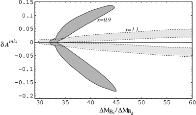
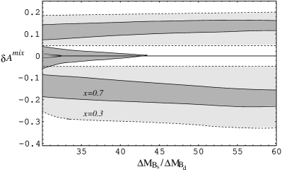
Next we analyze the possible deviations of the $CP$ asymmetries in $B\to\phi K$ from the SM expectation and the relation to the Bssubscript๐ต๐‘ B_{s}-Bยฏssubscriptยฏ๐ต๐‘ \bar{B}_{s} mass difference which is also altered by the insertions. In Fig.ย 2 we plot the correlation between the Bssubscript๐ต๐‘ B_{s}-Bยฏssubscriptยฏ๐ต๐‘ \bar{B}_{s} mass difference and $\delta A^{mix}\equiv A^{mix}-A^{mix,SM}$. We scan over the input SUSY parameters in the ranges

$\displaystyle\tilde{m}\in[250,1000]{\hbox{GeV}}$ (46)
$\displaystyle|(\delta^{d}_{23})_{LL}|\in[0,1]$ (47)
$\displaystyle\arg(\delta^{d}_{23})_{LL}\in[0,2\pi]\;,$ (48)

for different values of $x_{\tilde{g}\tilde{q}}$, the gluino-squark mass ratio. We require each point to satisfy the Bโ†’Xsโ€‹ฮณโ†’๐ตsubscript๐‘‹๐‘ ๐›พB\to X_{s}\gamma ${95\%\ \mathrm{C.L.}}$ constraint and to give a Bssubscript๐ต๐‘ B_{s}-Bยฏssubscriptยฏ๐ต๐‘ \bar{B}_{s} mass difference in the range 30โ‰คXsโ€‹dโ‰ค6030subscript๐‘‹๐‘ ๐‘‘6030\leq X_{sd}\leq 60. The various regions correspond to the limiting case: for a given ratio $x_{\tilde{g}\tilde{q}}$, no point lays outside them. For $x_{\tilde{g}\tilde{q}}\geq 1$ we find that the deviations from the $SM$ expectation remain below 0.05. For smaller values of $x_{\tilde{g}\tilde{q}}$ much larger and thus observable contributions are possible. This strong dependence on the ratio between the gluino and squark masses is due to the particular dependence of the loop functions on $x_{\tilde{g}\tilde{q}}$. Moreover, the presence of definite bands in the [Xsโ€‹d,ฮดโ€‹Amโ€‹iโ€‹x]subscript๐‘‹๐‘ ๐‘‘๐›ฟsuperscript๐ด๐‘š๐‘–๐‘ฅ[X_{sd},\delta A^{mix}] plane is due to an interplay between the Bโ†’Xsโ€‹ฮณโ†’๐ตsubscript๐‘‹๐‘ ๐›พB\to X_{s}\gamma constraint and the requirement of fixed ฮ”โ€‹MBsฮ”subscript๐‘€subscript๐ต๐‘ \Delta M_{B_{s}}.

As previously stated, $\delta A^{mix}$ measures the deviation of the mixing-induced $CP$ asymmetry from the standard model prediction. Since all new physics in the $B_{d}$-$\bar{B}_{d}$ mixing amplitude will affect the $CP$ asymmetries in the decays $B\to J/\Psi K$ and $B\to\phi K$ in the same way, $\delta A^{mix}$ is equal to $\sin 2(\beta+\theta_{d}+\theta_{A})-\sin 2(\beta+\theta_{d})$ where $\theta_{d}$ can be generated by other SUSY couplings that we do not consider here and $\theta_{A}$ is the phase of the $B\to\phi K$ decay amplitude. In other words, $\delta A^{mix}$ is the difference between the mixing-induced $CP$ asymmetries in the decays $B\to J/\Psi K$ and $B\to\phi K$ (see also the discussion in Sec.ย 2).

The new weak phases in the $B\to\phi K$ amplitude also leads to a non vanishing direct $CP$ asymmetry, $A^{dir}$, which can be measured for instance in decays of charged $B$-mesons. This asymmetry depends crucially on the presence of a strong rescattering phase, provided by the term $P$ of Eq.ย (17). Nevertheless, we find that the new physics contributions to the two asymmetries are strongly correlated. This can be understood as follows. Let us parametrize the $B\to\phi K$ decay amplitude as $A_{1}e^{i\phi_{1}}e^{i\delta_{1}}+A_{2}e^{i\phi_{2}}e^{i\delta_{2}}$ where $\phi_{i}$ and $\delta_{i}$ are weak and strong phases respectively; note that this parametrization is arbitrary but that all physical observables do not depend on its choice. In the SUSY model that we consider, the weak phases $\phi_{i}$ are entirely due to the imaginary part of the mass insertions. Using the above parametrization, we find that the ratio $A^{dir}/\delta A^{mix}$ has an extremely tiny dependence on the phases $\phi_{i}$; therefore, the correspondence between $A^{dir}$ and $\delta A^{mix}$ is almost one-to-one. In Fig.ย 3, we explicitely show this correlation.

Refer to caption
Refer to caption
Figure 1: Constraints on the complex mass insertions $(\delta^{d}_{23})_{LL}$ and $(\delta^{d}_{23})_{LR}$ coming from โ„ฌโ€‹(Bโ†’Xsโ€‹ฮณ)โ„ฌโ†’๐ตsubscript๐‘‹๐‘ ๐›พ{\cal B}(B\to X_{s}\gamma). We consider $m_{\tilde{g}}^{2}/\tilde{m}^{2}=1$. The contours scale as $\tilde{m}^{2}$. In the plot we explicitly show the cases $\tilde{m}=250,500{\hbox{GeV}}$.
Refer to caption
Refer to caption
Figure 2: Correlation between the Bssubscript๐ต๐‘ B_{s}โ€“Bยฏssubscriptยฏ๐ต๐‘ \bar{B}_{s} mass difference and the possible deviations $\delta A^{mix}$ of the mixingโ€“induced $CP$ asymmetry from the SM expectation. The various regions correspond to different values of $x_{\tilde{g}\tilde{q}}$.
Refer to caption
Figure 3: Correlation between $\delta A^{mix}$ and the direct $CP$ asymmetry $A^{dir}$.

5 Conclusions

We considered the effects of sizeable flavour changing entries in the squark matrices on bโ†’sโ†’๐‘๐‘ b\to s transitions. In particular we allowed for complex values of the relevant off-diagonal elements.

We first investigated the bounds that these entries must obey in order to satisfy the bโ†’sโ€‹ฮณโ†’๐‘๐‘ ๐›พb\to s\gamma data. Fig.ย 1 shows that the inclusion of complex values for the mass insertion parameters strongly enlarges their allowed regions. In fact, the absolute values of the insertions can be much larger than in the existing literature where only real couplings were considered. Moreover, there are interesting correlations between real and imaginary parts which may give important hints on the structure of the underlying theory.

We then considered the influence of the new terms on the $CP$-violating asymmetry in the decays $B\to\phi K$ and on the Bssubscript๐ต๐‘ B_{s}-Bยฏssubscriptยฏ๐ต๐‘ \bar{B}_{s} mixing (the $B_{d}$-$\bar{B}_{d}$ mixing is not affected by the terms we are interested in). In Fig.ย 2, we plot the deviation $\delta A^{mix}$ of the mixing-induced $CP$ asymmetry in $B\to\phi K$ from the SM expectation versus the ratio Xsโ€‹dsubscript๐‘‹๐‘ ๐‘‘X_{sd}. We see that $\delta A^{mix}$ can reach the $20\%$ level in some corners of the parameter space; on the other hand, deviations of order $O(10\%)$ are easily possible with moderately light squark and gluino masses. Note that such large contributions are possible only for configurations in which $m_{\tilde{g}}\lesssim m_{\tilde{q}}$. In a similar fashion, Fig.ย 3 shows that the direct $CP$ asymmetry $A^{dir}$ can receive contributions of the same order of magnitude. We stress that in this framework effects on $B\to J/\Psi K$ decays are expected to be tiny.

The Bssubscript๐ต๐‘ B_{s}-Bยฏssubscriptยฏ๐ต๐‘ \bar{B}_{s} ฮ”โ€‹MBsฮ”subscript๐‘€subscript๐ต๐‘ \Delta M_{B_{s}} is very sensitive to the mass insertions we consider, while $\Delta M_{B_{d}}$ remains unaffected. This implies that the determination of $V_{td}$ from ratio ฮ”โ€‹MBs/ฮ”โ€‹MBdฮ”subscript๐‘€subscript๐ต๐‘ ฮ”subscript๐‘€subscript๐ต๐‘‘\Delta M_{B_{s}}/\Delta M_{B_{d}} may be misleading. Moreover, as it follows from Fig.ย 2 and 3, an experimental determination of ฮ”โ€‹MBsฮ”subscript๐‘€subscript๐ต๐‘ \Delta M_{B_{s}} in excess with respect to the SM prediction together with sizeable $\delta A^{mix}$ and $A^{dir}$ would be strong signatures in favour of this kind of models. During the next year, the $B$-factories BABAR and BELLE will gather enough luminosity to study the $CP$ asymmetries in $B\to\phi K$ decays and will test this class of SUSY models soon.

Acknowledgments

E.L. acknowledges financial support from the Alexander Von Humboldt Foundation. D.W. is partially supported by Schweizerischer Nationalfonds.

References

  • [1] K.ย Ackerstaff etย al. [OPAL Collaboration], Eur. Phys. J. C5 (1998) 379.
    T.ย Affolder etย al. [CDF Collaboration], Phys. Rev. D61 (2000) 072005.
    C.ย A. Blocker [CDF Collaboration], To be published in the proceedings of 3rd Workshop on Physics and Detectors for DAPHNE (DAPHNE 99), Frascati, Italy, 16-19 Nov 1999.
    R.ย Barate etย al. [ALEPH Collaboration], Phys. Lett. B492 (2000) 259.
    B. Aubert et. al., [BABAR collaboration], Phys. Rev. Lett. 87 (2001) 091801.
    K. Abe et. al., [BELLE collaboration], Phys. Rev. Lett. 87 (2001) 091802.
  • [2] S.ย Mele, Phys. Rev. D59 (1999) 113011.
    S.ย Plaszczynski and M.-H. Schune, (1999), hep-ph/9911280.
    M.ย Bargiotti etย al., Riv. Nuovo Cim. 23N3 (2000) 1.
    A.ย Ali and D.ย London, Eur. Phys. J. C18 (2001) 665.
    M.ย Ciuchini etย al., (2000), JHEP 0107 (2001) 013.
    A.ย J. Buras, (2001), hep-ph/0101336.
    D.ย Atwood and A.ย Soni, Phys. Lett. B508 (2001) 17.
    A.ย Hocker, H.ย Lacker, S.ย Laplace, and F.ย L. Diberder, Eur. Phys. J. C 21 (2001) 225.
  • [3] W. S. Hou, 4th International Workshop on Particle Physics Phenomenology, Kaohsiung, Taiwan, China, 18-21 Jun 1998 and Workshop on CP Violation, Adelaide, Australia, 3-8 Jul 1998. Published in *Adelaide 1998, CP violation* 13-22, hep-ph/9902382.
  • [4] Y. Nir, Lectures given at 27th SLAC Summer Institute on Particle Physics: CP Violation in and Beyond the Standard Model (SSI 99), Stanford, California, 7-16 Jul 1999, hep-ph/9911321.
    Y. Grossmann and M. Worah, Phys. Lett. B395 (1997) 241.
  • [5] R. Fleischer and T. Mannel, Phys. Lett. B506 (2001) 311.
    R. Fleischer and T. Mannel, Phys. Lett. B511 (2001) 240.
  • [6] M.ย Ciuchini, G.ย Degrassi, P.ย Gambino, and G.ย F. Giudice, Nucl. Phys. B534, 3 (1998).
    A.ย Ali and D.ย London, Eur. Phys. J. C9, 687 (1999).
    A.ย Ali and D.ย London, Phys. Rept. 320, 79 (1999).
    A.ย J. Buras etย al., Phys. Lett. B500, 161 (2001).
    A.ย J. Buras and R.ย Buras, Phys. Lett. B501, 223 (2001).
    A.ย Bartl etย al., (2001), hep-ph/0103324.
    A.ย J. Buras and R.ย Fleischer, (2001), hep-ph/0104238.
  • [7] A.ย Ali and E.ย Lunghi, hep-ph/0105200.
    A.ย J.ย Buras, P.ย H.ย Chankowski, J.ย Rosiek and L.ย Slawianowska, hep-ph/0107048.
  • [8] V. Barger etย al., Phys. Rev. D64 (2001) 056007.
  • [9] J. Donoghue, H.P. Nilles and D. Wyler, Phys. Lett. B128 (1983) 55.
  • [10] A. Masiero, F. Borzumati, S. Bertolini and G. Ridolfi, Nucl. Phys. B353 (1991) 591.
  • [11] F. Borzumati et. al., Phys. Rev. D62 (2001) 075005.
  • [12] T. Besmer, C. Greub and T. Hurth, Nucl. Phys. B609 (2001) 359.
  • [13] Y. Grossman, M. Neubert and A. Kagan JHEP 9910 (1999) 029.
  • [14] G. Barenboim, J. Bernabeu and M. Raidal, Phys. Rev. Lett 80 (1998) 4625.
  • [15] B. Aubert et. al., BABAR collaboration, hep-ex/0105001.
  • [16] N. G. Deshpande and X. G. He, Phys. Lett. B336 (1994) 471.
  • [17] R.ย Barate etย al. [ALEPH Collaboration], Phys. Lett. B429 (1998) 169.
    K.ย Abe et al. [BELLE Collaboration], Phys. Lett. B511 (2001) 151.
    D.ย Cassel [CLEO Collaboration], talk presented at the XX International Symposium on Lepton and Photon Interactions at High Energies, Rome, Italy, Jul. 23-28, 2001. (To be published in the proceedings).
    J. Nash, [BABAR Collaboration], talk presented at the XX International Symposium on Lepton and Photon Interactions at High Energies, Rome, Italy, Jul. 23-28, 2001. (To be published in the proceedings).
  • [18] A. Kagan and M. Neubert, Eur. Phys. J. C7 (1999) 5.
  • [19] A. Kagan and M. Neubert, Phys. Rev. D58 (1998) 094012.
  • [20] F. Gabbiani, E. Gabrielli, A. Masiero and L. Silvestrini, Nucl. Phys. B477 (1996) 321.
  • [21] A. Ahrib, C. K. Chua and W. S. Hou, hep-ph/0104122.