Equation of state of strongly coupled
QCD at finite density

Abstract

Using an effective strongly coupled lattice QCD Hamiltonian and Wilson fermions we calculate the equation of state for cold and dense quark matter by constructing an ansatz which exactly diagonalizes the Hamiltonian to second order in field operators for all densities. This ansatz obeys the free lattice Dirac equation with a chemical potential term and a mass term which is interpreted as the dynamical quark mass. We find that the order of chiral phase transition depends on the values of input parameters. In the phase with spontaneously broken chiral symmetry the quark Fermi sea has negative pressure indicating its mechanical instability. This result is in qualitative agreement with those obtained using continuum field theory models with four–point interactions.

1 Introduction

Simulating finite density QCD is one of the outstanding problems in lattice gauge theory [1]. Because of the sign problem no reliable numerical simulations of finite density QCD with three colors exist even in the strong coupling limit [2]. This is a rather frustrating situation in view of the current intense interest in finite density QCD fueled by the phenomenology of heavy ion collisions, neutron stars, early universe and color superconductivity. Therefore even a qualitative description of strongly coupled QCD at finite density using field theoretical methods is quite welcome.

Strongly coupled QCD at finite quark chemical potential $\mu$ has previously been studied analytically both in the Euclidean [4, 5, 6] and in the Hamiltonian [7, 8] formulations. Except for [7], the consensus is that at zero or low temperatures strong coupling QCD undergoes a first order chiral phase transition from the broken symmetry phase below a critical chemical potential $\mu_{C}$ to a chirally symmetric phase above $\mu_{C}$. In this work we calculate the equation of state of strongly coupled QCD at finite $\mu$ using Wilson fermions and show that in the phase with spontaneously broken chiral symmetry the quark Fermi sea has negative pressure indicating its mechanical instability. This result is in qualitative agreement with those obtained using continuum field theory models with four–point interactions [9, 10].

2 Effective Hamiltonian and the ansatz for finite $\mu$

We begin by defining our effective Hamiltonian for strongly coupled QCD which was first derived by Smit [11]. Henceforth we adopt the notation of Smit [11], set the lattice spacing to unity ($a=1$) and work in momentum space. The charge conjugation symmetric form of Smit’s effective Hamiltonian with a chemical potential $\mu_{0}$ in momentum space is

$$H_{\rm eff} = \frac{1}{2}\sum_{\vec{p}}\biggl{[}M_{0}\left(\gamma_{0}\right)_{\sigma\nu}-\mu_{0}\delta_{\sigma\nu}\biggr{]}\biggl{[}\bigl{(}\Psi^{\dagger}_{a\alpha}\bigr{)}_{\sigma}(\vec{p}\,),\bigl{(}\Psi_{a\alpha}\bigr{)}_{\nu}(-\vec{p}\,)\biggr{]}_{-}$$ (1)

$$-\frac{K}{8N_{\rm c}}\sum_{\vec{p}_{1},\ldots,\vec{p}_{4}}\sum_{l=1}^{3}\delta_{\vec{p}_{1}+\cdot\cdot\cdot+\vec{p}_{4},\vec{0}}\Biggl{[}e^{i((\vec{p}_{1}+\vec{p}_{2})\cdot\hat{n}_{l})}+e^{i((\vec{p}_{3}+\vec{p}_{4})\cdot\hat{n}_{l})}\Biggr{]}$$

$$\!\!\!\!\!\!\!\!\!\!\!\!\!\!\!\otimes\Biggl{[}\left(\Sigma_{l}\right)_{\sigma\nu}\bigl{(}\Psi^{\dagger}_{a\alpha}\bigr{)}_{\sigma}(\vec{p}_{1}\,)\bigl{(}\Psi_{b\alpha}\bigr{)}_{\nu}(\vec{p}_{2}\,)-\left(\Sigma_{l}\right)^{\dagger}_{\sigma\nu}\bigl{(}\Psi_{a\alpha}\bigr{)}_{\nu}(\vec{p}_{1}\,)\bigl{(}\Psi^{\dagger}_{b\alpha}\bigr{)}_{\sigma}(\vec{p}_{2}\,)\Biggr{]}$$

$$\!\!\!\!\!\!\!\!\!\!\!\!\!\!\!\otimes\Biggl{[}\left(\Sigma_{l}\right)^{\dagger}_{\gamma\delta}\bigl{(}\Psi^{\dagger}_{b\beta}\bigr{)}_{\gamma}(\vec{p}_{3}\,)\bigl{(}\Psi_{a\beta}\bigr{)}_{\delta}(\vec{p}_{4}\,)-\left(\Sigma_{l}\right)_{\gamma\delta}\bigl{(}\Psi_{b\beta}\bigr{)}_{\delta}(\vec{p}_{3}\,)\bigl{(}\Psi^{\dagger}_{a\beta}\bigr{)}_{\gamma}(\vec{p}_{4}\,)\Biggr{]}$$

where $\left(\Sigma_{l}\right)=-i\left(\gamma_{0}\gamma_{l}-ir\gamma_{0}\right)$ with the Wilson parameter $r$ taking on values between 0 and 1. In the above Hamiltonian color, flavor and Dirac indices are denoted by $(a,b)$, $(\alpha,\beta)$ and $(\sigma,\nu,\gamma,\delta)$, respectively, and summation convention is implied. Three of the four parameters in this theory are the Wilson parameter $r$, the current quark mass $M_{0}$ and the effective coupling constant $K$ which behaves as $1/g^{2}$ with $g$ being the QCD coupling constant. The fourth parameter $\mu_{0}$ is in general not the total chemical potential $\mu_{\rm tot}$ of the interacting many body system. As shown below the interaction will induce a contribution to $\mu_{\rm tot}$ which is momentum dependent. We shall therefore refer $\mu_{0}$ as the ”bare” chemical potential.

Our strategy is to construct an ansatz which obeys the equation of motion corresponding to $H_{\rm eff}$ at finite $\mu$ and use it to calculate the equation of state of cold and dense quark matter. In free space this ansatz has the same structure as the free lattice Dirac field and obeys the free lattice Dirac equation with a mass term which is interpreted as the dynamical quark mass [12]. Temporarily dropping color and flavor indices, this ansatz is given by

$$\Psi_{\nu}(t,\vec{p}\,)=b(\vec{p}\,)\xi_{\nu}(\vec{p}\,)e^{-i\omega(\vec{p}\,)t}+d^{\dagger}(-\vec{p}\,)\eta_{\nu}(-\vec{p}\,)e^{+i\omega(\vec{p}\,)t}$$ (2)

The annihilation operators for particles, $b$, and anti–particles, $d$, annihilate an interacting vacuum state and obey the free fermion anti–commutation relations. The properties of the spinors $\xi$ and $\eta$ are given in [12]. The equation of motion for a free lattice Dirac field fixes the excitation energy $\omega(\vec{p}\,)$ to be

$$\omega(\vec{p}\,)=\left(\sum_{l}{\rm sin}^{2}(\vec{p}\cdot\hat{n}_{l})+M^{2}(\vec{p}\,)\right)^{1/2}$$ (3)

where $M(\vec{p}\,)$ plays the role of the dynamical quark mass or, equivalently, the chiral gap.

We now introduce temperature $T$ and $\mu$ simulatneously into our formalism and take the $T\rightarrow 0$ limit to construct an ansatz for finite $\mu$. This is accomplished by subjecting the $b$ and $d$ operators in Eq. (2) to a generalized thermal Bogoliubov transformation as in thermal field dynamics [13]

$$b(\vec{p}\>) = \alpha_{p}B(\vec{p}\>)-\beta_{p}\tilde{B}^{\dagger}(-\vec{p}\>)$$ (4)

$$d(\vec{p}\>) = \gamma_{p}D(\vec{p}\>)-\delta_{p}\tilde{D}^{\dagger}(-\vec{p}\>)$$ (5)

The thermal field operators $B$ and $\tilde{B}^{\dagger}$ annihilate a quasi–particle and create a quasi–hole at finite $T$ and $\mu$, respectively, while $D$ and $\tilde{D}^{\dagger}$ are the annihilation operator for a quasi–anti–particle and creation opertor for a quasi–anti–hole, respectively.

The thermal annihilation operators annihilate the interacting thermal vacuum state $|\,{\cal G}(T,\mu)\rangle$ for each $T$ and $\mu$.

$$B(\vec{p}\>)|\,{\cal G}(T,\mu)\rangle=\tilde{B}(\vec{p}\>)|\,{\cal G}(T,\mu)\rangle = 0$$ (6)

$$D(\vec{p}\>)|\,{\cal G}(T,\mu)\rangle=\tilde{D}(\vec{p}\>)|\,{\cal G}(T,\mu)\rangle = 0$$ (7)

The thermal doubling of the Hilbert space accompanying the thermal Bogoliubov transformation is implicit in Eqs. (6) and (7) where a vacuum state which is annihilated by thermal operators $B$, $\tilde{B}$, $D$ and $\tilde{D}$ is defined. Since we shall be working only in the space of quantum field operators it is not necessary to specify the structure of $|\,{\cal G}(T,\mu)\rangle$.

The thermal operators satisfy the Fermion anti–commutation relations just as the $b$ and $d$ operators in the free space ansatz. The coefficients of the transformation are $\alpha_{p}=\sqrt{1-n_{p}^{-}}$, $\beta_{p}=\sqrt{n_{p}^{-}}$, $\gamma_{p}=\sqrt{1-n_{p}^{+}}$ and $\delta_{p}=\sqrt{n_{p}^{+}}$, where $n_{p}^{\pm}=[e^{(\omega_{p}\pm\mu)/(k_{B}T)}+1]^{-1}$ are the Fermi distribution functions for particles and anti–particles. They are chosen so that the total particle number densities are given by

$$n_{p}^{-} = \langle\,{\cal G}(T,\mu)|b^{\dagger}(\vec{p}\>)b(\vec{p}\>)|\,{\cal G}(T,\mu)\rangle$$ (8)

$$n_{p}^{+} = \langle\,{\cal G}(T,\mu)|d^{\dagger}(\vec{p}\>)d(\vec{p}\>)|\,{\cal G}(T,\mu)\rangle$$ (9)

Hence in this approach temperature and chemical potential are introduced simultaneously through the coefficients of the thermal Bogoliubov transformation and are treated on an equal footing. We stress that the chemical potential appearing in the Fermi distribution functions is the total chemcial potential of the interacting many body system which is not necessarily equal to the bare chemical potential $\mu_{0}$ appearing in the effective Hamiltonian in Eq. (1).

We demand that our ansatz satisfies the equation of motion corresponding to the free lattice Dirac Hamiltonian with a chemical potential term. This Hamiltonian is given by

$$H^{0} = \frac{1}{2}\sum_{\vec{p}}\Biggl{[}-\sum_{l}{\rm sin}(\vec{p}\cdot\hat{n}_{l})(\gamma_{0}\gamma_{l})_{\sigma\nu}+M(\vec{p}\,)(\gamma_{0})_{\sigma\nu}-\mu_{\rm tot}\delta_{\sigma\nu}\Biggr{]}$$ (10)

$$\;\;\;\;\;\;\otimes\Bigg{[}\Psi_{\sigma}^{\dagger}(t,\vec{p}\,),\Psi_{\nu}(t,\vec{p}\,)\Biggr{]}_{-}$$

As in [12] the mass $M(\vec{p}\,)$ will be identified with the chiral gap while $\mu_{\rm tot}$ is the total chemical potential mentioned above. In the $T\rightarrow 0$ limit the excitations of anti–holes are supressed which amount to setting $\gamma_{p}=1$ and $\delta_{p}=0$ in Eq. (5). Thus our ansatz at finite $\mu_{\rm tot}$ is given by

$$\Psi_{\nu}(t,\vec{p}\>) = \biggl{[}\alpha_{p}B(\vec{p}\>)-\beta_{p}\tilde{B}^{\dagger}(-\vec{p}\>)\biggr{]}\xi_{\nu}(\vec{p}\,)e^{-i[\omega(\vec{p}\,)-\mu_{\rm tot}]t}$$ (11)

$$\;\;\;\;\;\;\;\;\;\;\;\;\;\;\;\;\;\;\;\;+\;\;\gamma_{p}D^{\dagger}(-\vec{p}\>)\eta_{\nu}(-\vec{p}\,)e^{+i[\omega(\vec{p}\,)+\mu_{\rm tot}]t}$$

The spinors $\xi$ and $\eta$ obey the same properties as in free space and the excitation energy $\omega(\vec{p}\,)$ has the same form as in Eq. (3).

Two quantities of interest that can be calculated in a straightforward manner using Eq. (11) are the quark number density $\langle\bar{\Psi}\gamma_{0}\Psi\rangle$ and the chiral condensate $\langle\bar{\Psi}\Psi\rangle$. They are found to be

$$\langle\bar{\Psi}\gamma_{0}\Psi\rangle = \sum_{\vec{p}}\beta_{p}^{2}$$ (12)

and

$$\langle\bar{\Psi}\Psi\rangle = -\sum_{\vec{p}}\alpha_{p}^{2}\frac{M(\vec{p}\,)}{\omega(\vec{p}\,)}$$ (13)

We see immediately from Eq. (13) that the chiral condensate is proportional to the dynamical quark mass and therefore can clearly be identified as being the order parameter for the chiral phase transition at finite density.

3 Application of the Equation of Motion

3.1 The Gap Equation and the Induced Chemical Potential

We proceed by using the ansatz shown in Eq. (11) in our effective Hamiltonian to determine the equation of motion. This is accomplished by exploiting the fact that our ansatz satisfies the equation of motion corresponding to the free Hamiltonian at finite $\mu$ given in Eq. (10). We therefore have the relation

$$:\Bigl{[}\bigl{(}\Psi_{a\alpha}\bigr{)}_{\nu}(t,\vec{q}\,),H^{0}\Bigr{]}_{-}:\;\;\;\;=\;\;\;\;:\Bigl{[}\bigl{(}\Psi_{a\alpha}\bigr{)}_{\nu}(t,\vec{q}\,),H_{\rm eff}\Bigr{]}_{-}:$$ (14)

where the symbol : : denotes normal ordering with respect to the thermal vacuum $|\,{\cal G}(T=0,\mu)\rangle$. Evaluating both sides of Eq. (14) and equating terms which are linear in the field operators we obtain

$$\!\!\!\!\!\!\!\!\!\!\!\!\!\!\!\Bigl{[}\sum_{l}{\rm sin}(\vec{q}\cdot\hat{n}_{l})(\gamma_{0}\gamma_{l})_{\nu\delta}+M(\vec{q}\,)(\gamma_{0})_{\nu\delta}-\mu_{\rm tot}\delta_{\nu\delta}\Bigr{]}\bigl{(}\Psi_{a\alpha}\bigr{)}_{\delta}(t,\vec{q}\,)=$$ (15)

$$\Bigl{[}A(\vec{q}\,)(\gamma_{0}\gamma_{l})_{\nu\delta}+B(\vec{q}\,)(\gamma_{0})_{\nu\delta}+C(\vec{q}\,)\delta_{\nu\delta}\Bigr{]}\bigl{(}\Psi_{a\alpha}\bigr{)}_{\delta}(t,\vec{q}\,)$$

The momentum dependent coefficients $B$ and $C$ in Eq. (15) determine the gap equation and the total chemical potential, respectively.

$$M(\vec{q}\,) = B(\vec{q}\,)$$ (16)

$$= M_{0}+\frac{3}{2}K(1-r^{2})\sum_{\vec{p}}\left(1-\beta_{p}^{2}\right)\frac{M(\vec{p}\,)}{\omega(\vec{p}\,)}$$

$$\!\!\!\!\!\!\!\!\!\!+\;\;\frac{1}{N_{\rm c}}K\sum_{\vec{p},l}\left(1-\beta_{p}^{2}\right)\frac{M(\vec{p}\,)}{\omega(\vec{p}\,)}\Biggl{\{}8r^{2}\cos(\vec{p}\cdot\hat{n}_{l})\cos(\vec{q}\cdot\hat{n}_{l})$$

$$\!\!\!\!\!\!\!\!\!\!-\;\frac{1}{2}(1+r^{2})\cos(\vec{p}+\vec{q}\,)\cdot\hat{n}_{l}\Biggr{\}}$$

$$\mu_{\rm tot}(\vec{q}\,) = -C(\vec{q}\,)$$ (17)

$$= \!\!\mu_{0}\!+\!\frac{1}{4}\frac{K}{N_{c}}\!\sum_{\vec{p},l}\beta_{p}^{2}\Bigl{[}2N_{c}\left(1+r^{2}\right)-2\left(1-r^{2}\right){\rm cos}\left(\vec{p}+\vec{q}\,\right)\Bigr{]}$$

The structure of the gap equation Eq. (16) is very similar to that in free space ($\beta^{2}_{p}=0$) found in [12]. The dynamical quark mass is a constant to lowest order in $N_{c}$ but becomes momentum dependent once $1/N_{c}$ correction is taken into account. We see from Eq. (17) that the total chemical potential is a sum of the bare chemical potential $\mu_{0}$ and a momentum dependent contribution generated by the interaction. Because of this induced chemical potential Eqs. (16) and (17) are coupled and must be solved self–consistently. It should be noted that this shifting of the bare chemical potential by the interaction is not a new effect. In the Nambu–Jona–Lasinio model [14] within the Hartree–Fock approximation and at finite $T$ and $\mu$, the interaction induces a contribution to the total chemcial potential which is proportional to the number density [15].

Figure 1: a) Dynamical quark mass versus the total chemical potential to lowest order in $N_{c}$ for $K$ = 0.8 (solid line) and 1.0 (dashed line) with $r$ = 0. A first order chiral phase transition takes places in both cases with a critical chemical potential of $\mu_{C}$ = 1.042 and 1.329 for $K$ = 0.8 and 1.0, respectively. b) Dynamical quark mass versus the total chemical potential to lowest order in $N_{c}$ for $K$ = 0.8 (solid line) and 0.9 (dashed line) with $r$ = 0.25. A second order chiral phase transition takes place for $K$ = 0.8 with a critical chemical potential of $\mu_{C}$ = 0.836 while the transition is first order for $K$ = 0.9 with $\mu_{C}$ = 1.086. The current quark mass is set to zero ($M_{0}=0$) in all cases.

Solutions for the coupled equations Eqs. (16) and (17) to lowest order in $N_{C}$ are shown in Figure 1 where we present the dynamical quark masses as functions of the total chemical potential for various combinations of the Wilson parameter $r$ and the coupling constant $K$ with a vanishing current quark mass. As shown in Figure 1a we find first order chiral phase transitions when $r$ = 0 (i.e. with naive fermions) with critical chemical potentials of $\mu_{C}\approx 1.04$ and 1.33 for $K$ = 0.8 and 0.9, respectively. As far as the order of the phase transition is concerned, our results agree with those obtained using the Euclidean formulation with Kogut–Susskind fermions [4, 5, 6] and also with a recent result obtained with naive fermions ($r$ = 0) in a Hamiltonian formulation [8]. However we disagree with the result of Le Yaouanc et al. [7] who find a second order chiral phase transition using the same effective Hamiltonian as in this work and naive fermions.

For $r$ = 0.25 we see from Figure 1b that the phase transition can be either first or second order depending on the value of the effective coupling constant $K$. When $K$ = 0.8 we find a second order phase transition with $\mu_{C}\approx 0.84$ while if the coupling constant is increased to 0.9 the phase transition becomes first order with a larger critical chemical potential of $\mu_{C}\approx 1.09$. It would be interesting to investigate whether the approaches adapted in [7] and [8] to study strongly coupled QCD in the Hamiltonian lattice formulation using naive fermions would result in a similar behaviour of the order of the phase transition when extended to $r>0$. Finally, we note that for both $r$ = 0 and 0.25 the value of the critical chemical potential increases as $K$ is increased. The same behaviour has been observed in [6].

3.2 Off–diagonal Hamiltonian and the Vacuum Energy Density

The off–diagonal Hamiltonian which is bilinear in field creation and annihilation operators may be written as

$$H_{\rm off}|\,{\cal G}(0,\mu)\rangle=\sum_{\vec{q}}F(\vec{q}\,)B^{\dagger}_{\alpha,a}(\vec{q}\,)D^{\dagger}_{\alpha,a}(-\vec{q}\,)|\,{\cal G}(0,\mu)\rangle$$ (18)

where $F(\vec{q}\,)$ is a scalar function of $\vec{q}$. We see from Eq. (18) that the elementary excitation of the effective Hamiltonian involves color singlet (quasi–) quark–anti–quark excitations coupled to zero total three momentum. With the use of the equation of motion and properties of $\eta$ spinor [12] it can be shown analytically that $H_{\rm off}|\,{\cal G}(0,\mu)\rangle=0$ for all $\mu$. Therefore our ansatz exactly diagonalizes the effective Hamiltonian to second order in field operators for all densities.

Having verified that our ansatz diagonalizes the second order Hamiltonian we are in a position to evaluate the vacuum energy density. Using Eq. (15) we find

$$\frac{1}{V}\langle{\cal G}(0,\mu)|H_{\rm eff}|\,{\cal G}(0,\mu)\rangle=$$ (19)

$$-2N_{c}\sum_{\vec{p}}\Biggl{\{}\alpha_{p}^{2}\Biggl{[}\frac{3}{2}K(1+r^{2})+\omega(\vec{p}\,)+\frac{M(\vec{p}\,)}{\omega(\vec{p}\,)}M_{0}$$

$$-\frac{1}{N_{c}}\frac{K}{2}(1-r^{2})\sum_{\vec{q}}\cos(\vec{p}+\vec{q}\,)\cdot\hat{n}_{l}-\mu_{\rm tot}\Biggr{]}+(1+\beta_{p}^{2})\mu_{0}\Biggr{\}}$$

From Eq. (19) we can evaluate the difference of the vacuum energy densities in the Wigner–Weyl ($M(\vec{q}\,)=0$) and Nambu–Goldstone ($M(\vec{q}\,)\neq 0$) phases of the theory. We find

$$\Delta E=\frac{1}{V}\langle{\cal G}|H_{\rm eff}|\,{\cal G}\rangle|_{M(\vec{q}\,)=0}-\frac{1}{V}\langle{\cal G}|H_{\rm eff}|\,{\cal G}\rangle|_{M(\vec{q}\,)\neq 0}>0$$ (20)

and therefore the true ground state of our interacting many body system is in the phase with broken chiral symmetry.

4 Equation of State

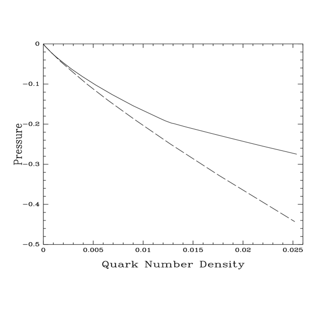
Figure 2: Pressure versus the quark number density to lowest order in $N_{c}$ for $K$ = 0.8 (solid line) and 0.9 (dashed line) with $M_{0}=0$ and $r$ = 0.25. Quark number densities at the chiral phase transtion point are $n_{q}$ = 0.013 and 0.025 for $K$ = 0.8 and 0.9, respectively.

Having solved the gap equation for the dynamical quark mass we proceed to determine the equation of state of cold and dense quark matter. We present results obtained with a vanishing current quark mass and Wilson fermions for $r$ = 0.25 to leading order in $N_{c}$ since in this case we observe both first and second order chiral phase transitions. The pressure of the cold and dense quark matter is obtained by numerically evaluating the thermodynamic potential density. In Figure 2 we plot the pressure as functions of quark number density for $K$ = 0.8 and 0.9. In both cases we find the pressure to be negative in the broken symmetry phase and therefore the quark Fermi sea is mechanically unstable with an imaginary speed of sound.

Our conclusion regarding the quark matter stability at finite density is consistent with results obtained using the Nambu–Jona–Lasinio model [9] and the effective instanton induced ’t Hooft interaction model [10]. In both [9] and [10] mean field calculations show that cold and dense quark matter is unstable in the phase with spontaneously broken chiral symmetry and lead the authors to speculate the formation of quark droplets reminiscent of the MIT bag model.

5 Conclusion

In this work we studied strongly coupled QCD in the Hamiltonian lattice formalism at finite density using Wilson fermions. Starting from an effective Hamiltonian we constructed and an ansatz which exactly diagonalizes the Hamiltonian to second order in field operators for all densities. This ansatz obeys the free lattice Dirac equation with a chemical potential term and a mass term which plays the role of the dynamical quark mass. This mass and the total chemical potential of the interacting many body system were determined to lowest order in $N_{c}$ by solving a coupled set of equations obtained from the equation of motion. We find a first order chiral phase transition with naive fermions while the order of the phase transition can be either first or second for Wilson fermions. As in earlier studies using continuum four–fermion interaction models we find that the quark Fermi sea is mechanically unstable in the phase with broken chiral symmetry. Our results for the equation of state of cold and dense quark matter should certainly be verified in any future numerical simulation of finite density QCD.

References

- [1] M. Creutz, Lattice gauge theory: A retrospective, Los Alamos Archives arXiv:hep-lat/0010047.
- [2] R. Aloisio, V. Azcoiti, G. Di Carlo, A. Galante and A.F. Grillo, Nucl. Phys. B 564 (2000) 489.
- [3] J.B. Kogut, D.K. Sinclair, S.J. Hands and S.E. Morrison, Two–colour QCD at non–zero quark number density, arXiv:hep-lat/0105026.
- [4] P.H. Damgaard, D. Hochberg, N. Kawamoto, Phys. Letts. B 158 (1985) 239.
- [5] E.–M. Ilgenfritz and J. Kripfganz, Z. Phys. C 29 (1985) 79.
- [6] N. Bilić, K. Demeterfi and B. Petersson, Nucl. Phys. B 377 (1992) 651.
- [7] A. Le Yaouanc, L. Oliver, O. Pène and J.–C. Raynal, M. Jarfi and O. Lazrak, Phys. Rev. D 37 (1986) 3691; 37 (1986) 3702.
- [8] E.B. Gregory, S.–H. Guo, H. Kröger and X.–Q. Luo, Phys. Rev. D 62 (2000) 054508.
- [9] M. Buballa, Nucl. Phys. A 611 (1996) 393.
- [10] M. Alford, K. Rajagopal and F. Wilczek, Phys. Letts. B 422 (1998) 247.
- [11] J. Smit, Nucl. Phys. B 175 (1980) 307.
- [12] Y. Umino, Phys. Letts. B 492 (2000) 385.
- [13] H. Umezawa, H. Matsumoto and M. Tachiki, Thermo Field Dynamics and Condensed States, (North–Holland, Amsterdam, 1982); H. Umezawa, Advanced Field Theory, (AIP, New York, 1992).
- [14] Y. Nambu and G. Jona–Lasinio, Phys. Rev. 122 (1961) 345; 124 (1961) 246.
- [15] M. Asakawa and K. Yazaki, Nucl. Phys. A 504 (1989) 668. Also see the review article by S.P. Klevansky, Rev. Mod. Phys. 64 (1992) 649.