Scale-independent mixing angles

A radiatively-corrected mixing angle has to be independent of the choice of renormalization scale to be a physical observable. At one-loop in $\overline{\rm MS}$ , this occurs for a particular value, $p_{*}$, of the external momentum in the two-point functions used to define the mixing angle: $p_{*}^{2}=(M_{1}^{2}+M_{2}^{2})/2$, where $M_{1,2}$ are the physical masses of the two mixed particles. We examine two important applications of this to the Minimal Supersymmetric Standard Model: the mixing angle for a) neutral Higgs bosons and b) stops. We find that this choice of external momentum improves the scale independence (and therefore provides a more reliable determination) of these mixing angles.

September 2001

IEM-FT-220/01

IFT-UAM/CSIC-01-26

hep-ph/0109126

In Quantum Field Theory renormalized using dimensional regularization and minimal subtraction [1] (or modified minimal subtraction, $\overline{\rm MS}$  [2]), the parameters of the model at hand (say the Standard Model, SM or some extension therof) depend on an arbitrary renormalization scale, $Q$. The running of these parameters with $Q$ is governed by the corresponding renormalization group equations (RGEs). Physical observables, on the other hand, cannot depend on the arbitrary scale $Q$, and the relations that link physical quantities to the running $\overline{\rm MS}$  parameters are of obvious importance in order to make contact between theory and experiment.

Two familiar examples in the SM concern the Higgs and top quark masses. The relation between the top-quark pole mass, $M_{t}$, and the running top Yukawa coupling, $h_{t}(Q)$, (or alternatively the running top quark mass) is of the form

$$h_{t}(Q)=2^{3/4}G_{F}^{1/2}M_{t}\left[1+\delta_{t}(Q,p^{2}=M_{t}^{2})\right]\ ,$$ (1)

where $G_{F}$ is Fermi’s constant and the function $\delta_{t}$, which contains the radiative corrections, depends explicitly on $Q$ and is evaluated on-shell, i.e. at external momentum satisfying $p^{2}=M_{t}^{2}$. This function $\delta_{t}$ is known up to three loops in QCD [3, 4] and one loop in electroweak corrections [5]. The relation between the Higgs boson pole mass and its quartic self-coupling $\lambda(Q)$ is similar to (1):

$$\lambda(Q)={1\over\sqrt{2}}G_{F}M_{h}^{2}\left[1+\delta_{h}(Q,p^{2}=M_{h}^{2})\right]\ .$$ (2)

The function $\delta_{h}$ was obtained at one loop in ref. [6].

The scale dependence of the exact functions $\delta_{t}(Q)$ and $\delta_{h}(Q)$ in eqs. (1) and (2) must be such that it exactly compensates the scale-dependence of the couplings $h_{t}(Q)$ and $\lambda(Q)$, in such a way that $M_{t}$ and $M_{h}$ are scale-independent. As shown by these examples, in practice we can only calculate $\delta_{t}(Q)$ and $\delta_{h}(Q)$ in some approximation (say up to some finite loop order) and, in general, there is some residual scale dependence left. In fact, choosing a particular value $Q^{*}$ of the renormalization scale by demanding that the residual scale dependence is minimized (this can be done with different levels of sophistication, see [7]) gives in general a good approximation to the full result, or allows a good estimate of higher order corrections. Often there is some physical reason for the particular value $Q^{*}$ chosen (e.g. $Q^{*}$ might be some average of the masses of the virtual particles that dominate the loop corrections, or the typical energy scale of the process studied), but this is not necessarily the case always [4, 8].

A physical mass is defined at the pole of the corresponding propagator and therefore the external momentum in (1) and (2) is set to the physical mass. As we remind in section 1, this choice ensures that the scale dependence in equations like (1) and (2) is the same on both sides, leading to a scale-independent definition of the physical mass (up to the residual dependences due to higher order corrections just mentioned). The purpose of this letter is to address the problem of how to obtain a scale-independent mixing angle between two particles with the same quantum numbers, so that a convenient definition of such angles can be achieved. We will show that relations similar to (1) and (2) can be found that relate ‘physical’ and ‘running’ mixing angles. Then we show that, at one loop, a scale-independent mixing angle in $\overline{\rm MS}$  is possible for a very particular choice of external momentum, $p_{*}$, in the self-energies that contribute to radiative corrections, with

$$p_{*}^{2}={1\over 2}(M_{1}^{2}+M_{2}^{2})\ ,$$ (3)

where $M_{1}$ and $M_{2}$ are the physical masses of the two particles that mix.

In section 1 we present the general derivation of the momentum scale $p_{*}$ for the simple case of the mixing angle between two scalar fields. We apply this general result to two important cases with phenomenological interest in the Minimal Supersymmetric Standard Model (MSSM): first to the stop mixing in section 2 and then to the mixing between the two ${\cal CP}$-even Higgs scalars in section 3. We end with some conclusions in section 4.

1. We start by proving the scale-independence (at one-loop) of the pole-mass for a single scalar field, $\varphi$, with Lagrangian

$${\cal L} = {1\over 2}\partial_{\mu}\varphi_{0}\partial^{\mu}\varphi_{0}-{1\over 2}m_{0}^{2}\varphi_{0}^{2}+...$$ (4)

$$= {1\over 2}\partial_{\mu}\varphi\partial^{\mu}\varphi-{1\over 2}m^{2}\varphi^{2}+{1\over 2}\delta Z_{\varphi}\partial_{\mu}\varphi\partial^{\mu}\varphi-{1\over 2}\delta m^{2}\varphi^{2}+...\ ,$$

where $\varphi_{0},m_{0}$ ($\varphi,m$) are bare (renormalized, say in $\overline{\rm MS}$ -scheme) quantities and $\delta Z_{\varphi},\delta m^{2}$ are counterterms. They are related by

$$\varphi_{0} = \left(1+{1\over 2}\delta Z_{\varphi}\right)\varphi\ ,$$ (5)

$$m_{0}^{2} = m^{2}+\delta m^{2}-\delta Z_{\varphi}m^{2}\ .$$ (6)

The quantities $\varphi$ and $m^{2}$ depend on the renormalization scale $Q$ through $\delta Z_{\varphi}$ and $\delta m^{2}$:

$${d\ln\varphi\over d\ln Q^{2}} \equiv \gamma=-{1\over 2}{d\delta Z_{\varphi}\over d\ln Q^{2}}\ ,$$ (7)

$${dm^{2}\over d\ln Q^{2}} \equiv \beta_{m^{2}}=-{d\delta m^{2}\over d\ln Q^{2}}+m^{2}{d\delta Z_{\varphi}\over d\ln Q^{2}}\equiv\beta_{m^{2}}^{0}-2\gamma m^{2}\ .$$ (8)

The relation between the one-loop bare and renormalized inverse propagators, $\Gamma_{0}(p^{2})$ and $\Gamma(p^{2})$ respectively, is

$$\Gamma(p^{2})\equiv p^{2}-m^{2}+\Pi(p^{2})=(1+\delta Z_{\varphi})\Gamma_{0}(p^{2})=(1+\delta Z_{\varphi})[p^{2}-m_{0}^{2}+\Pi_{0}(p^{2})]\ ,$$ (9)

where $\Pi_{0}(p^{2})$ $[\Pi(p^{2})]$ is the bare (renormalized) one-loop self-energy for external momentum $p^{2}$. From (9) we can obtain the renormalization-scale dependence of the $\overline{\rm MS}$ -renormalized self-energy:

$${\partial\Pi(p^{2})\over\partial\ln Q^{2}}=\beta_{m^{2}}^{0}-2\gamma p^{2}\ .$$ (10)

The physical mass, $M$, is defined as the real part of the propagator pole. Therefore, $M$ is given by

$$M^{2}\equiv m^{2}-\Pi(p^{2}=M^{2})\ .$$ (11)

From this, using (8) and (10) we find

$${dM^{2}\over d\ln Q^{2}}={dm^{2}\over d\ln Q^{2}}-{d\Pi(M^{2})\over d\ln Q^{2}}=\left.2\gamma(m^{2}-p^{2})\right|_{p^{2}=M^{2}}+{\cal{O}}(\hbar^{2})\ .$$ (12)

For the on-shell choice $p^{2}=M^{2}$, noting that $M^{2}=m^{2}+{\cal{O}}(\hbar)$, eq. (12) is zero at one-loop order (of course the proof can be extended to all orders).

The scale-independence just proved also holds in the case of mixed fields. Consider two scalar fields, $\varphi_{1}$ and $\varphi_{2}$, with the same quantum numbers, so that they can mix. Their inverse propagator, for external momentum $p$, is a $2\times 2$ matrix which at one-loop order has the form

$${\bf\Gamma}(p^{2})\ \equiv p^{2}\ {\bf I_{2}}-[{\bf m^{2}}-{\bf\Delta}(p^{2})]=\left[\begin{array}[]{cc}p^{2}-m_{11}^{2}+\Delta_{11}&-m_{12}^{2}+\Delta_{12}\\[5.69054pt] -m_{21}^{2}+\Delta_{21}&p^{2}-m_{22}^{2}+\Delta_{22}\end{array}\right]\ .$$ (13)

where ${\bf m^{2}}$ is the $\overline{\rm MS}$ -renormalized (‘tree-level’) mass matrix and ${\bf\Delta}(p^{2})$ contains the one-loop radiative corrections. In $\overline{\rm MS}$ -scheme (or for supersymmetric theories $\overline{\rm DR}$  [9], the SUSY version of $\overline{\rm MS}$ , with dimensional reduction instead of dimensional regularization), the elements of ${\bf m^{2}}$ depend implicitly on the renormalization scale $Q$ through an equation of the form:

$${dm_{ij}^{2}\over d\ln Q^{2}}\equiv\beta_{ij}\equiv\beta_{ij}^{0}-\sum_{k}\left(\gamma_{ik}m_{kj}^{2}+\gamma_{kj}m_{ik}^{2}\right).$$ (14)

In (14) we have written separately the contributions from wave-function renormalization, with the anomalous dimensions $\gamma_{ij}$ defined by

$${d\varphi_{i}\over d\ln Q^{2}}\equiv\sum_{k}\gamma_{ik}\varphi_{k}\ .$$ (15)

The fact that $\gamma_{ij}$ is in general a $2\times 2$ matrix reflects the possibility of having kinetic mixing between the two scalar fields.

The one-loop radiative corrections to the inverse propagator, collected in ${\bf\Delta}$, depend explicitly on the external momentum $p$ and on $\ln Q^{2}$. In fact, the elements of that matrix satisfy

$${\partial\Delta_{ij}\over\partial\ln Q^{2}}=\beta_{ij}^{0}-2p^{2}\gamma_{ij}\ .$$ (16)

The two mass eigenvalues are the poles of ${\bf\Gamma}^{-1}(p^{2})$, that is, the solutions $p^{2}=M^{2}_{i}$ ($i=1,2$) of the equation

$${\mathrm{D}et}\ [Re\ {\bf\Gamma}(p^{2})]=p^{4}-p^{2}\ {\mathrm{T}r}\ [{\bf M^{2}}(p^{2})]+{\mathrm{D}et}\ [{\bf M^{2}}(p^{2})]=0\ ,$$ (17)

where ${\bf M^{2}}(p^{2})\equiv{\bf m^{2}}-{\bf\Delta}(p^{2})$. To find $M_{1,2}^{2}$, eq. (17) has to be solved self-consistently to the order we work (one-loop). It is easy to show that the mass eigenvalues, $M^{2}_{i}$, are indeed scale-independent at one loop. Taking the derivative of eq. (17) with respect to $\ln Q^{2}$, with $p^{2}=M_{i}^{2}$, we find

$${dM_{i}^{2}\over d\ln Q^{2}}\propto\left[-M_{i}^{2}{d\ {\mathrm{T}r}\ {\bf M^{2}}\over d\ln Q^{2}}+{d\ {\mathrm{D}et}\ {\bf M^{2}}\over d\ln Q^{2}}\right]\ .$$ (18)

Using eqs. (14) and (16) to evaluate $dM_{ij}^{2}/d\ln Q^{2}$ and making a loop expansion, the right-hand side of eq. (18) is shown to be proportional to

$$m_{i}^{4}-m_{i}^{2}\ {\mathrm{T}r}\ {\bf m^{2}}+{\mathrm{D}et}\ {\bf m^{2}}\ ,$$ (19)

where $m_{i}^{2}$ is an eigenvalue of the tree-level mass matrix, and therefore must satisfy the secular equation ${\mathrm{D}et}[m_{i}^{2}{\bf I_{2}}-{\bf m^{2}}]=0$, so that (19) is zero [and then also (18) vanishes]. This establishes the scale independence of $M_{i}^{2}$ at one-loop. In summary, this agrees nicely with the well known result that a physical definition of the radiatively corrected masses, $M_{i}^{2}$, requires the self-energy corrections $[{\bf\Delta}(p^{2})]$ to be evaluated on-shell, i.e. at $p^{2}=M_{i}^{2}$.

Besides the particle masses, ${\bf\Gamma}(p^{2})$ in eq. (13) contains also information on the mixing between the two particles. We can define the radiatively-corrected mixing angle, $\alpha(p^{2})$, as the angle of the rotation that diagonalizes the mass matrix ${\bf M^{2}}={\bf m^{2}}-{\bf\Delta}(p^{2})$:

$$\tan[2\alpha(p^{2})]\equiv{\sqrt{4\left[m_{12}^{2}-\Delta_{12}(p^{2})\right]\left[m_{21}^{2}-\Delta_{21}(p^{2})\right]}\over m_{11}^{2}-m_{22}^{2}+\Delta_{22}(p^{2})-\Delta_{11}(p^{2})}\ .$$ (20)

Proceeding like we did for the masses, the scale-dependence of $\tan[2\alpha(p^{2})]$ can be extracted from eqs. (14,16). At one-loop order, it is simply given by

$${d\tan 2\alpha\over d\ln Q^{2}}\propto\left[2p^{2}-{\mathrm{T}r}\ {\bf m^{2}}\right]\ .$$ (21)

From this result we conclude that a scale-independent mixing angle can be defined at external momentum

$$p_{*}^{2}\equiv{1\over 2}(M_{1}^{2}+M_{2}^{2})\ .$$ (22)

This is the simple result we wanted to prove. We choose to define $p_{*}$ in terms of the radiatively corrected masses in analogy with the on-shell definition of physical masses. Eq. (21) involves tree-level masses and cannot be used to justify this choice, although it is of course compatible with it at one-loop. Besides the analogy with OS masses, numerical examples in later sections will provide good support for this choice.

In applying the previous prescription to gauge theories one should worry about the gauge-independence of the mixing-angle definition. We expect our prescription to be amenable of improvement in order to make it also gauge-independent (along the lines of [10]). The results of such analysis will be presented elsewhere [11]. For our current purposes notice that in the examples of the following sections the scale dependence of the parameters that enter the definition of the mixing angle is very mildly affected by electroweak gauge couplings, so that it is a good approximation for our numerical analyses to neglect them.

2. In the context of the MSSM, one particular case in which the previous discussion is of interest concerns the stop sector. This sector consist of two scalars, $\tilde{t}_{L,R}$, supersymmetric partners of the top quark which, after electroweak symmetry breaking, can mix. Their tree-level mass matrix is given by

$${\bf m}^{2}_{\tilde{t}}\ \simeq\ \left[\begin{array}[]{cc}M_{L}^{2}+m_{t}^{2}&m_{t}X_{t}\\[5.69054pt] m_{t}X_{t}^{*}&M_{R}^{2}+m_{t}^{2}\end{array}\right]\ ,$$ (23)

where $M_{L}$ ($M_{R}$) is the squared soft mass for $\tilde{t}_{L}$ ($\tilde{t}_{R}$), $m_{t}$ is the top mass and $X_{t}\equiv A_{t}+\mu^{*}/\tan\beta$, with $A_{t}$ the soft trilinear coupling associated to the top Yukawa coupling, $\mu$ the Higgs mass parameter in the superpotential and $\tan\beta$ the ratio between the vacuum expectation values of the two Higgs doublets of the model. In (23) we have neglected gauge couplings, which give a small contribution through $D$-terms. The one-loop self-energy corrections for stops in the MSSM, ${\bf\Delta}_{\tilde{t}}(p^{2})$, can be found in [12, 13].

The stop mixing angle, $\theta_{t}(p^{2})$, including one-loop radiative corrections, can be defined for any value of the external momentum $p$ as the angle of the basis rotation which diagonalizes ${\bf M}^{2}_{\tilde{t}}\equiv{\bf m}^{2}_{\tilde{t}}-{\bf\Delta}_{\tilde{t}}(p^{2})$. Following section 1, we define a scale-independent mixing angle ${\tilde{\theta}}_{t}\equiv\theta_{t}(p_{*}^{2})$, for $p_{*}^{2}=(M_{\tilde{t}_{1}}^{2}+M_{\tilde{t}_{2}}^{2})/2$, where $M_{\tilde{t}_{i}}^{2}$ are the (one-loop) stop mass eigenvalues.

In figures 1.a and 1.b, we illustrate the scale dependence of $\tan 2\theta_{t}(p^{2})$ in the range 100 GeV $\leq Q\leq$ 1 TeV for different values of the external momentum $p$. We choose the following stop parameters: $M_{L}=1500$ GeV, $M_{R}=300$ GeV, $X_{t}=1$ TeV and $\tan\beta=10$ for figure 1.a, and $M_{L}=M_{R}=X_{t}=1$ TeV, $\tan\beta=10$ for figure 1.b (these are values at the electroweak scale, $Q\sim 100$ GeV). We work in the approximation of neglecting all couplings other than the strong gauge coupling and the top and bottom Yukawa couplings for the RG evolution of the tree-level matrix (23). The scale evolution of this matrix is considered only at one-loop leading-log order, that is

$$m_{ij}^{2}(Q)\simeq m_{ij}^{2}(Q_{0})+\beta_{ij}\ln{Q^{2}\over Q_{0}^{2}}\ ,$$ (24)

with $Q_{0}=100$ GeV. The quantities $\beta_{ij}$ depend also on the soft mass of right-handed sbottoms, $M_{D}$, on the soft trilinear coupling, $A_{b}$, associated to the bottom Yukawa coupling in the superpotential and on the gluino mass, $M_{g}$. We take $M_{D}=M_{g}=1$ TeV and $A_{b}=0$. The upper (lower) curves correspond to $p^{2}$ equal to the heavier (lighter) mass eigenvalue (of the radiatively-corrected mass matrix) while the flat curves in-between have $p^{2}=p_{*}^{2}\equiv(M_{\tilde{t}_{1}}^{2}+M_{\tilde{t}_{2}}^{2})/2$. The improvement in scale independence is dramatic when this last choice is made. The difference in $\tan 2\theta_{t}$ due to different choices of the external momentum can be a $\sim 5-7\%$ effect in the case of figure 1.a and much larger for 1.b (depending strongly on the value chosen for the renormalization scale).

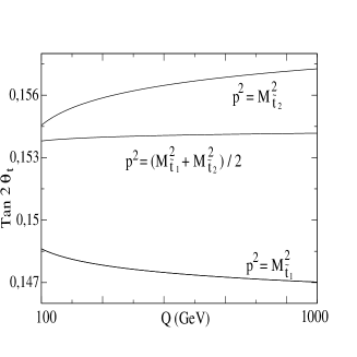
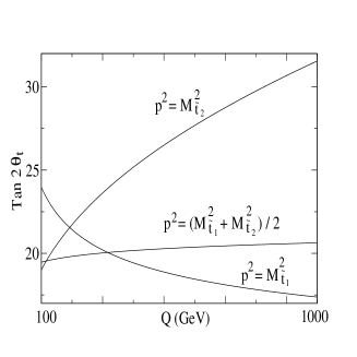
Figure 1:

Scale dependence of the stop mixing-angle $\theta_{t}(p^{2})$ for different values of the external momentum $p$ as indicated. Figure 1.a (left plot) has $M_{L}=1500$ GeV, $M_{R}=300$ GeV, $Xt=1$ TeV while figure 1.b (right plot) has $M_{L}=M_{R}=X_{t}=1$ TeV. In both cases $\tan\beta=10$.

Once a scale-independent mixing angle ${\tilde{\theta}}_{t}$ has been obtained, we can also define a scale-independent, ’on-shell’, stop mixing parameter, $X_{t}^{OS}$, by the relation (already used in [14])

$$\sin 2{\tilde{\theta}}_{t}\equiv{2M_{t}X_{t}^{OS}\over M_{\tilde{t}_{1}}^{2}-M_{\tilde{t}_{2}}^{2}}\ ,$$ (25)

where $M_{t}$ is the pole mass of the top quark.

3. Another sector of the MSSM in which radiative corrections and mixing effects are quite relevant is the Higgs sector, in particular for the mixing between the two neutral Higgses (we assume ${\cal CP}$ is approximately conserved in the Higgs sector so that only two ${\cal CP}$-even states can mix. If this were not the case, similar analyses would be possible). In the $\{H_{1}^{0},H_{2}^{0}\}$ basis, the Higgs mass matrix, corrected at one loop, is

$${\bf M}^{2}_{H}\ \simeq\ \left[\begin{array}[]{cc}m_{A}^{2}s_{\beta}^{2}+m_{Z}^{2}c_{\beta}^{2}-\Delta_{11}&-(m_{A}^{2}+m_{Z}^{2})s_{\beta}c_{\beta}-\Delta_{12}\\[5.69054pt] -(m_{A}^{2}+m_{Z}^{2})s_{\beta}c_{\beta}-\Delta_{21}&m_{A}^{2}c_{\beta}^{2}+m_{Z}^{2}s_{\beta}^{2}-\Delta_{22}\end{array}\right]\ .$$ (26)

In this expression, $m_{Z}$ and $m_{A}$ are the $\overline{\rm DR}$  masses of the $Z^{0}$ gauge boson and the pseudoscalar Higgs, $A^{0}$, respectively and we use the shorthand notation $s_{\beta}=\sin\beta$, etc. The diagonal one-loop self-energy corrections include a piece from Higgs tadpoles (see e.g. ref. [12]) which ensure that Higgs vacuum expectations values minimize the one-loop effective potential. With this definition, the parameter $\tan\beta$ has the usual RGE in terms of the Higgs anomalous dimensions:

$${d\tan\beta\over d\ln Q^{2}}\equiv\gamma_{2}-\gamma_{1}\ ,$$ (27)

with $\gamma_{i}\equiv d\ln H_{i}^{0}/d\ln Q^{2}$. In spite of this small complication present in the Higgs sector, the general derivation given in section 1 gets through also in this case: we get a scale-independent Higgs mixing angle, $\alpha$, with the external momentum taken as $p^{2}=p_{*}^{2}=(M_{h}^{2}+M_{H}^{2})/2$, where $M_{h}$ and $M_{H}$ are the masses of the light and heavy ${\cal CP}$-even Higgses respectively.

To show this, we plot $\tan[2\alpha(p^{2})]$ in figures 2 and 3 as a function of the renormalization scale, with 100 GeV $\leq Q\leq$ 1 TeV, for different choices of parameters. In figure 2 we take $m_{A}=500$ GeV, with $\tan\beta=3$ in the upper-left plot, $\tan\beta=10$ in the upper-right one and $\tan\beta=40$ in the lower plot. For the rest of parameters we take $X_{t}=0$, $X_{b}\equiv A_{b}+\mu\tan\beta=0$ (i.e. diagonal squark masses), $Y_{t}\equiv A_{t}-\mu\tan\beta=0$, and $M_{L}=M_{R}=M_{D}=1$ TeV. Just like in the previous section, we have made several approximations for our numerical examples: we neglect all couplings other than the top and bottom Yukawa couplings (here the strong coupling does not enter in one-loop corrections) and consider the RG evolution of the tree-level piece of (26) only at one-loop leading-log level [like in eq. (24)].

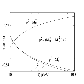
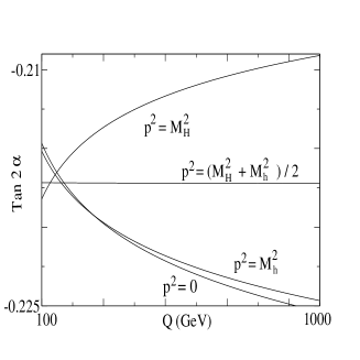
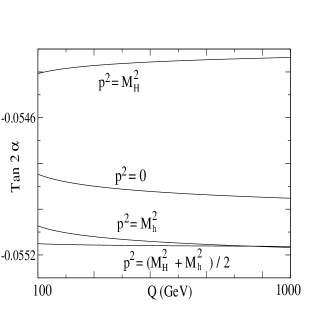
Figure 2:

Scale-dependence of the momentum-dependent Higgs mixing-angle $\alpha(p^{2})$ for $p^{2}$ values as indicated. All figures have $m_{A}=500$ GeV, $X_{t}=X_{b}=Y_{t}=0$ and $M_{L}=M_{R}=M_{D}=1$ TeV, while $\tan\beta$ is 3 for the upper-left plot, 10 for the upper-right one and 40 for the lower plot.

From figure 2 we see that the choice $p^{2}=p_{*}^{2}=(M_{h}^{2}+M_{H}^{2})/2$ indeed improves significantly the scale-independence of the Higgs mixing angle $\alpha(p^{2})$. In these plots we compare this choice of external momentum with three other possibilities: $p^{2}$ equal to one of the Higgs masses squared ($M_{h}^{2}$ or $M_{H}^{2}$, radiatively corrected) or $p^{2}=0$. The possibility $p^{2}=M_{h}^{2}$ has been used frequently in the literature to define the Higgs mixing angle. The same can be said of $p^{2}=0$, which is the choice made when radiative corrections are extracted from the effective potential only, without correcting for wave-function renormalization effects.

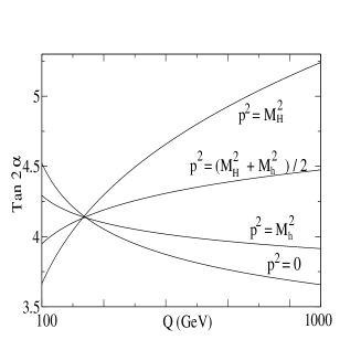
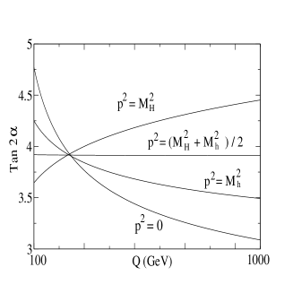
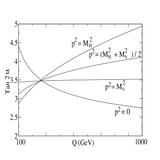
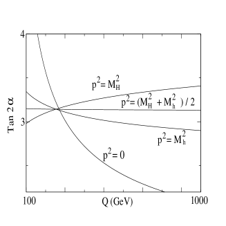
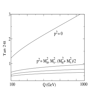
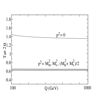
Figure 3:

Scale dependence of the momentum-dependent Higgs mixing-angle $\alpha(p^{2})$ for $p^{2}$ values as indicated. All figures have $m_{A}=120$ GeV; the parameter $\tan\beta$ is $3,10,40$ from top to bottom plots while $X_{t}=X_{b}=Y_{t}=0$ and $M_{L}=M_{R}=M_{D}=1$ TeV. Left plots use a purely one-loop definition of $\alpha$ while those in the right use a improved definition, as described in the text.

The left column of plots in figure 3 presents the same comparison between different choices of external momentum in the definition of the mixing angle $\alpha$ but for a lower value of the pseudoscalar mass: $m_{A}=120$ GeV, with the rest of parameters chosen as in figure 2. The parameter $\tan\beta$ is 3 for the upper(-left) plot, 10 for the middle one and 40 for the lower plot. (In the plots for $\tan\beta=40$, curves with higher $p^{2}$ correspond to lower values of $\tan[2\alpha(p^{2})]$.) It is clear from this figure that, although $p^{2}=p_{*}^{2}$ is somewhat better than other choices, there is some residual scale-dependence left. In this case with low $m_{A}$, the effect of higher order corrections is not negligible, and eventually such effects should be taken into account if a better scale stability of the mixing angle is required.

To do that, one should go beyond the one-loop approximation used so far. To identify more clearly the origin of the residual scale dependence let us write explicitly [using (14), (16) and (24)] the elements of the radiatively-corrected mass matrix. Assume for simplicity that $\gamma_{ij}=\gamma_{i}\delta_{ij}$ and $m_{12}^{2}=m_{21}^{2}$. For the diagonal elements one has (in one-loop leading-log approximation):

$$M_{ii}^{2}(Q)\simeq m_{ii}^{2}(Q_{0})-\Delta_{ii}(p,Q_{0})-2\gamma_{i}(m_{ii}^{2}-p^{2})\ln{Q^{2}\over Q_{0}^{2}}\ ,$$ (28)

and, for the off-diagonal element:

$$M_{12}^{2}(Q)\simeq m_{12}^{2}(Q_{0})-\Delta_{12}(p,Q_{0})-(\gamma_{1}+\gamma_{2})m_{12}^{2}\ln{Q^{2}\over Q_{0}^{2}}\ .$$ (29)

The scale at which the prefactors of the logarithmic terms should be evaluated is irrelevant for the one-loop leading-log approximation: different choices introduce differences only in higher order corrections. One may try to choose a scale that approximates well such corrections. One could also argue in favour of including in the prefactors of the logarithmic terms finite (non-logarithmic) radiative corrections. The key observation to improve the scale-independence of the mixing angle beyond one-loop is the following: if the matrix elements have the form

$$M_{ii}^{2}(Q) \simeq {\tilde{m}}_{ii}^{2}-2\gamma_{i}({\tilde{m}}_{ii}^{2}-p^{2})\ln{Q^{2}\over Q_{0}^{2}}\ ,$$ (30)

$$M_{12}^{2}(Q) \simeq {\tilde{m}}_{12}^{2}(Q_{0})-(\gamma_{1}+\gamma_{2})\tilde{m}_{12}^{2}\ln{Q^{2}\over Q_{0}^{2}}\ .$$ (31)

where ${\tilde{m}}_{ij}^{2}\equiv m_{ij}^{2}(Q_{0})+[{\mathrm{Q}-indep.\ loop\ corrections}]$, then it is straightforward to show that the mixing angle for the matrix with elements (30) and (31) is exactly scale-independent for $p^{2}=({\tilde{m}}_{11}^{2}+{\tilde{m}}_{22}^{2})/2$. Therefore, in order to improve over the one-loop leading-log result, we make the replacement

$$m_{ij}^{2}\rightarrow m_{ij}^{2}(Q_{0})-\Delta_{ij}(p,Q_{0})\ ,$$ (32)

in the logarithmic terms of (28) and (29). At this point one should worry about the choice of scale $Q_{0}$. However, eqs. (14) and (16) [with the replacement (32) made also in (14) for consistency] guarantee that the elements of the Higgs mass matrix, improved by (32), are independent of $Q_{0}$. We have checked numerically that the impact of the choice of $Q_{0}$ in the mixing angle is tiny.

The replacement (32) is similar to the use of improved masses in [16] for a numerically accurate calculation of radiatively corrected Higgs masses. It amounts to the inclusion of some one-loop corrections to Higgs masses in the determination of $p_{*}^{2}$. Note however that it does not correspond to the use of the full one-loop masses. Such choice would be consistent only if the Higgs self-energies were computed at two-loops. If that is not the case it does not give a better scale-independence than the advocated choice in (32). A consistent two-loop analysis of the scale-stability of mixing angles would be interesting but lies beyond the scope of the present paper.

The results for $\tan[2\alpha(p^{2})]$ after the improvement (32) are presented in the plots of the right column of figure 3. The parameters are the same as those chosen for the left plots, so that the improvement in scale stability can be appreciated by direct comparison: now the choice $p^{2}=p_{*}^{2}\equiv(M_{\tilde{t}_{1}}^{2}+M_{\tilde{t}_{2}}^{2})/2$ gives a perfectly scale-independent determination of $\alpha$. From these plots we also see that, at least for moderate values of $\tan\beta$, there is a particular value of the renormalization scale for which a) the mixing angle is nearly momentum independent and all curves are focused in one point and b) the corresponding value of the mixing angle is a good approximation to the scale independent result. Clearly, that choice of renormalization scale corresponds to a value for which the one-loop logarithmic radiative corrections are minimized. The existence of such a good choice of scale is not always guaranteed if the spectrum of the particles in the loops is widespread, case in which not all logarithms can be made small at a single renormalization scale.

4. The mixing angle between two scalar particles with the same quantum numbers, once radiative corrections are taken into account, depends on the renormalization scale and the external momentum. We have shown that, at one-loop, the scale dependence disappears for a particular choice of the external momentum, $p_{*}^{2}=(M_{1}^{2}+M_{2}^{2})/2$, where $M_{1,2}$ are the masses of the two particles. The particular momentum $p_{*}$ plays a role similar to the on-shell choice $p^{2}=M^{2}$ for the determination of a radiatively corrected physical mass $M$.

We have applied this prescription to two cases of interest in the Minimal Supersymmetric Standard Model: the mixing between stops and the ${\cal CP}$-even Higgs mixing. We have shown numerically that the advocated choice of momentum does indeed improve the scale independence of the one-loop corrected mixing angles in both cases. In the Higgs boson case, especially for low values of the pseudoscalar mass, we had to go beyond the one-loop approximation to get a satisfactory behaviour of the mixing angle, but this could be achieved easily by taking into account higher order corrections (in particular, one-loop non-logarithmic corrections to mass parameters in expression which were already of one-loop order). Therefore, our prescription could be very useful for a reliable determination of these mixing angles.

References

- [1] G. ’t Hooft, Nucl. Phys. B 61 (1973) 455.
- [2] W. A. Bardeen, A. J. Buras, D. W. Duke and T. Muta, Phys. Rev. D 18 (1978) 3998.
- [3] N. Gray, D. J. Broadhurst, W. Grafe and K. Schilcher, Z. Phys. C 48 (1990) 673.
-
[4]
K. G. Chetyrkin and M. Steinhauser,
Phys. Rev. Lett. 83 (1999) 4001
[hep-ph/9907509];
K. Melnikov and T. v. Ritbergen, Phys. Lett. B 482 (2000) 99 [hep-ph/9912391]. - [5] R. Hempfling and B. A. Kniehl, Phys. Rev. D 51 (1995) 1386 [hep-ph/9408313].
- [6] A. Sirlin and R. Zucchini, Nucl. Phys. B 266 (1986) 389.
-
[7]
G. Grunberg,
Phys. Lett. B 95 (1980) 70
[Erratum-ibid. B 110 (1980) 501];
Phys. Rev. D 29 (1984) 2315;
P. M. Stevenson, Phys. Lett. B 100 (1981) 61; Phys. Rev. D 23 (1981) 2916; Nucl. Phys. B 231 (1984) 65;
S. J. Brodsky, G. P. Lepage and P. B. Mackenzie, Phys. Rev. D 28 (1983) 228;
S. J. Brodsky and H. J. Lu, Phys. Rev. D 51 (1995) 3652 [hep-ph/9405218]. - [8] A. Ferroglia, G. Ossola and A. Sirlin, Nucl. Phys. B 560, 23 (1999) [hep-ph/9905442].
-
[9]
W. Siegel,
Phys. Lett. B 84 (1979) 193;
D. M. Capper, D. R. T. Jones and P. van Nieuwenhuizen, Nucl. Phys. B 167 (1980) 479;
I. Jack, D. R. T. Jones, S. P. Martin, M. T. Vaughn and Y. Yamada, Phys. Rev. D 50 (1994) 5481 [hep-ph/9407291]. - [10] Y. Yamada, Phys. Rev. D 64 (2001) 036008 [hep-ph/0103046].
- [11] J. R. Espinosa, I. Navarro and Y. Yamada, work in progress.
- [12] D. M. Pierce, J. A. Bagger, K. Matchev and R. Zhang, Nucl. Phys. B491 (1997) 3 [hep-ph/9606211].
- [13] A. Donini, Nucl. Phys. B467 (1996) 3 [hep-ph/9511289].
- [14] J. R. Espinosa and I. Navarro, Nucl. Phys. B 615 (2001) 82 [hep-ph/0104047].
-
[15]
P. Chankowski, S. Pokorski and J. Rosiek,
Nucl. Phys. B 423 (1994) 437
[hep-ph/9303309];
A. Dabelstein, Z. Phys. C 67 (1995) 495 [hep-ph/9409375];
A. Dabelstein, Nucl. Phys. B 456 (1995) 25 [hep-ph/9503443];
S. Heinemeyer, W. Hollik and G. Weiglein, Eur. Phys. J. C 9 (1999) 343 [hep-ph/9812472];
L. Shan, Eur. Phys. J. C 12 (2000) 113 [hep-ph/9807456]. - [16] A. Brignole, Phys. Lett. B 281 (1992) 284.
-
[17]
H. E. Haber and R. Hempfling,
Phys. Rev. D 48 (1993) 4280
[hep-ph/9307201];
M. Carena, J. R. Espinosa, M. Quirós and C. E. Wagner, Phys. Lett. B 355 (1995) 209 [hep-ph/9504316]. - [18] Y. Yamada, [hep-ph/9608382].
- [19] M. A. Díaz, [hep-ph/9705471].