Nonlinear Gluon Evolution in the Color Glass Condensate: II

Abstract

We complete the construction of the renormalization group equation (RGE) for the Color Glass Condenstate begun in Paper I. This is the equation which governs the evolution with rapidity of the statistical weight function for the color glass field. The coefficients in this equation — one-loop real and virtual contributions — are computed explicitly, to all orders in the color glass field. The resulting RGE can be interpreted as the imaginary-time evolution equation, with rapidity as the “imaginary time”, for a quantum field theory in two spatial dimensions. In the weak field limit it reduces to the BFKL equation. In the general non-linear case, it is equivalent to an equation by Weigert which summarizes in functional form the evolution equations for Wilson line operators previously derived by Balitsky and Kovchegov.

I Introduction

Hadronic scattering at high energy, or small Bjorken’s $x$, uncovers a novel regime of QCD where the coupling is small ($\alpha_{s}\ll 1$) but the parton densities are so large that conventional perturbation theory breaks down, via strong non-linear effects [1, 2, 3, 4, 5, 6, 7, 8, 9, 10]. In a previous paper [11], to be referred to as “Paper I” throughout this text, we have outlined the construction of an effective theory which is well suited to study the non-linear phenomena at small $x$ and has a transparent physical interpretation: It portrays the gluon component of the hadron wavefunction (the relevant component at small $x$) as a Color Glass Condensate (CGC). This is a multiparticle quantum state with high occupation numbers, but to the accuracy of interest it can be represented as a classical stochastic color field with a probability law determined by a functional Fokker-Planck equation.

The latter is a renormalization group equation (RGE) which shows how to construct the effective theory by integrating out quantum fluctuations in the background of a strong color field (the CGC). The non-linear effects included in the RGE via this background field describe interactions among the gluons produced in the quantum evolution towards small $x$. This leads to a non-linear generalization of the BFKL equation [12] whose general structure has been originally identified in Refs. [13], in an effort to give a field-theoretical justification to the McLerran-Venugopalan model for the gluon distribution of a large nucleus [5, 14, 15, 16]. But previous attempts [17] to compute the coefficients in this equation (beyond the linear, or BFKL, approximation [13]) have suffered from technical complications and, moreover, appear to be inconsistent with the results obtained from other perturbative approaches [18, 19, 20].

In this paper, we continue the analysis in Paper I and compute explicitly the coefficients in the RGE alluded to above. As recently reported in Ref. [21], the non-linear effects encoded in these coefficients lead to gluon saturation, that is, to a limitation on the maximum gluon density in the hadron wavefunction as $x\to 0$. In contrast to the linear BFKL equation, which predicts the exponential growth of the gluon distribution function with $\tau\equiv\ln(1/x)$, our corresponding result grows only linearly, and thus respects the unitarity bounds. This is consistent with a previous result by Mueller [7], and also with some recent analyses [22, 23, 24, 10] of the Balitsky–Kovchegov equations [18, 19], which are encoded too in our RGE [25] (see also Sect. V B below).

This paper is quite technical and relies heavily on the results of Paper I. To facilitate its reading and prepare the calculations to follow, it is convenient to summarize, in the remaining part of this Introduction, the general structure of the effective theory and its quantum evolution. In this introductory discussion, we shall follow the presentation in Paper I, to which the reader may refer for more details, but we shall also anticipate some of the results to be obtained later in this paper. The remaining sections are organized as follows: In Section II we present the explicit calculation of the “real correction’, i.e., the charge-charge correlator $\chi$ which plays the role of the diffusion kernel in the functional RGE. In Section III we do the same for the “virtual correction”, i.e., the one-point function $\sigma$ which plays the role of a force term. In Section IV, we present the final result for the RGE, and discuss its general structure and some of its remarkable properties. We emphasize, in particular, the Hamiltonian structure of this equation, and its relation with a similar equation by Weigert [20]. In Section V, we derive evolution equations for observables from the general RGE. In the weak field limit, we thus recover the BFKL equation for the unintegrated gluon distribution. In the general non-linear case, we obtain the coupled evolution equations for Wilson-line correlators originally derived by Balitsky and (in the large $N_{c}$ limit) also by Kovchegov. In Section VI we present conclusions and perspectives. Some explicit calculations, as well as the presentation of the background field gluon propagator, are deferred to the four Appendices.

A The effective theory for the CGC

The effective theory applies to gluon correlations in the hadron wavefunction as measured in deep inelastic scattering at small Bjorken’s $x$. It is formulated in the hadron infinite momentum frame, where small $x$ corresponds to soft longitudinal momenta $k^{+}=xP^{+}$, with $P^{+}$ the hadron momentum, and $x\ll 1$. The main physical assumption, which is a posteriori verified in the construction of the effective theory, is that the “fast” partons in the hadron wavefunction (i.e., the excitations with relatively large longitudinal momenta $p^{+}\gg k^{+}$) can be replaced, as far as their effects on the soft correlation functions are concerned, by a classical random color source $\rho^{a}(x)$, whose gross properties are determined by the kinematics.

The separation of scales in longitudinal momenta ($p^{+}\gg k^{+}$) implies a corresponding separation in (light-cone) energies ($p^{-}\sim p_{\perp}^{2}/2p^{+}\,\ll\,k^{-}\sim k_{\perp}^{2}/2k^{+}$), and therefore also in (light-cone) time scales: The lifetime $\Delta x^{+}\sim 1/k^{-}\propto k^{+}$ of the soft gluons is much shorter than the characteristic time scale $\sim 1/p^{-}\propto p^{+}$ for the dynamics of the fast partons. Thus, the latter appear to the soft gluons as nearly on-shell colored particles which propagate on the light-cone ($z\simeq t$, or $x^{-}\simeq 0$) with large $p^{+}$ momenta. The associated color charge density $\rho^{a}(x)$ is therefore static (i.e., independent of $x^{+}$), localized near the light-cone (within a small distance $\Delta x^{-}\sim 1/p^{+}\ll 1/k^{+}$), and random (since this is the instantaneous color charge in the hadron “seen” by the soft gluons at the arbitrary time of their emission). The correlations of $\rho$ are encoded in a gauge-invariant weight function $W_{\tau}[\rho]$. This is the probability density for having a color charge distribution with density $\rho_{a}(x^{-},{\bf x}_{\perp})$, normalized as:

$$\int{\cal D}\rho\,\,W_{\tau}[\rho]\,=\,1\,.$$ (1)

Note that we use the momentum-space rapidity $\tau\equiv\ln(P^{+}/k^{+})=\ln(1/x)$ to indicate the dependence of the weight function upon the soft scale $k^{+}$.

Thus, in this effective theory, the equal-time gluon correlation functions at the scale $k^{+}=xP^{+}$ are obtained as (with ${\vec{x}}\equiv(x^{-},{\bf x}_{\perp})$):

$$\langle A^{i}_{a}(x^{+},\vec{x})A^{j}_{b}(x^{+},\vec{y})\cdots\rangle_{\tau}\,=\,\int{\cal D}\rho\,\,W_{\tau}[\rho]\,{\cal A}_{a}^{i}({\vec{x}}){\cal A}_{b}^{j}({\vec{y}})\cdots\,,$$ (2)

where ${\cal A}_{a}^{i}\equiv{\cal A}_{a}^{i}[\rho]$ is the solution to the classical Yang-Mills equations with source $\rho_{a}$ :

$$(D_{\nu}F^{\nu\mu})_{a}(x)\,=\,\delta^{\mu+}\rho_{a}(x)\,,$$ (3)

in the light-cone (LC) gauge $A^{+}_{a}=0$, which is the gauge which allows for the most direct contact with the gauge-invariant physical quantities [8, 11]. For instance, the gluon distribution function ($\equiv$ the total number of gluons per unit rapidity with longitudinal momentum $k^{+}=xP^{+}$ and transverse momentum $k_{\perp}^{2}\leq Q^{2}$) is obtained as [8, 11]

$$xG(x,Q^{2}) = {1\over\pi}\int{d^{2}k_{\perp}\over(2\pi)^{2}}\,\Theta(Q^{2}-k_{\perp}^{2})\,\Bigl{\langle}\,|{\cal F}^{+i}_{a}(\vec{k})|^{2}\Bigr{\rangle}_{\tau}\,.$$ (4)

where ${\cal F}^{+i}_{a}=\partial^{+}{\cal A}^{i}_{a}$ is the electric field associated to the classical solution ${\cal A}_{a}^{i}[\rho]$, and $\vec{k}\equiv(k^{+},{\bf k}_{\perp})$ with $k^{+}=xP^{+}=P^{+}{\rm e}^{-\tau}$.

To deduce explicit expressions for these classical fields, it is preferable to express the LC-gauge solution ${\cal A}_{a}^{i}$ in terms of color source $\tilde{\rho}_{a}$ in the covariant gauge $\partial^{\mu}\tilde{A}_{\mu}=0$ (COV-gauge). This is possible since both the measure and the weight function in the functional integral (2) are gauge-invariant, so that the classical average can be done equally well by integrating over the COV-gauge $\tilde{\rho}$. In terms of this latter, the classical solution ${\cal A}_{a}^{\mu}[\tilde{\rho}]$ is known explicitly [11], and reads: ${\cal A}_{a}^{+}=0$ (the gauge condition), ${\cal A}^{-}_{a}=0$, and (in matrix notations appropriate for the adjoint representation: $\tilde{\rho}\equiv\tilde{\rho}_{a}T^{a}$, etc.)

$$\,{\cal A}^{i}\,(\vec{x}) = {i\over g}\,U(\vec{x})\,\partial^{i}U^{\dagger}(\vec{x}),$$ (6)

$$U^{\dagger}(x^{-},x_{\perp}) = {\rm P}\exp\left\{ig\int_{-\infty}^{x^{-}}dz^{-}\,{\alpha}(z^{-},x_{\perp})\right\},$$ (7)

$$-\nabla^{2}_{\perp}\alpha({\vec{x}}) = \tilde{\rho}(\vec{x}).$$ (8)

This is the gauge-transform, with gauge function $U(\vec{x})$, of the corresponding solution in the COV-gauge, which has only one non-trivial component: $\tilde{\cal A}^{\mu}_{a}=\delta^{\mu+}\alpha_{a}({\vec{x}})$. All the fields above are static, i.e., independent of $x^{+}$. Since $\tilde{\rho}$, and therefore $\alpha$, are localized at $\Delta x^{-}<1/k^{+}$, the associated field ${\cal A}^{i}$ appears effectively as a $\theta$–function :

$${\cal A}^{i}(x^{-},x_{\perp})\,\approx\,\theta(x^{-})\,{i\over g}\,V(\partial^{i}V^{\dagger})\,\equiv\,\theta(x^{-}){\cal A}^{i}_{\infty}(x_{\perp}),$$ (9)

to any probe with a much lower longitudinal resolution (i.e., with momenta $q^{+}\ll k^{+}$). On the same resolution scale:

$$U^{\dagger}(x^{-},x_{\perp})\,\approx\,\theta(x^{-})\,V^{\dagger}(x_{\perp})+\theta(-x^{-}),\qquad\,{\cal F}^{+i}(\vec{x})\,\approx\,\delta(x^{-})\,{\cal A}^{i}_{\infty}(x_{\perp}).$$ (10)

In the equations above, $V$ and $V^{\dagger}$ are the asymptotic values of the respective gauge rotations as $x^{-}\to\infty$ :

$$V^{\dagger}(x_{\perp})\,\equiv\,{\rm P}\exp\left\{ig\int_{-\infty}^{\infty}dz^{-}\,\alpha(z^{-},x_{\perp})\right\}.$$ (11)

In practice, $U(x^{-},x_{\perp})=V(x_{\perp})$ for any $x^{-}\gg 1/k^{+}$.

Note that the solution to the classical non-linear equation is known exactly, which makes this approach particularly convenient to study the non-linear physics at small $x$. The classical approximation should be indeed appropriate in this regime, which is characterized by weak coupling and large occupation numbers. On the other hand, the weight function $W_{\tau}[\rho]$ is obtained via a quantum calculation in which the quantum fluctuations with momenta $k^{+}\mathrel{\hbox to0.0pt{\raise 2.20013pt\hbox{$<$}\hss}{\lower 2.20013pt\hbox{$\sim$}}}p^{+}\mathrel{\hbox to0.0pt{\raise 2.20013pt\hbox{$<$}\hss}{\lower 2.20013pt\hbox{$\sim$}}}P^{+}$ are integrated out in layers of $p^{+}$, and in the background of the classical fields ${\cal A}^{i}$ [15, 13, 11]. This calculation captures the basic mechanism leading to large gluon densities — namely, the BFKL-type of evolution towards small $x$ —, while also including non-linear effects (i.e., rescatterings among the produced gluons) via the background fields. In the saturation regime, where one expects color fields as strong as ${\cal A}^{i}\sim 1/g$ (corresponding, via eq. (4), to gluon densities of order $1/\alpha_{s}$ [8, 15, 7, 21]), the background field calculation must be carried out exactly, i.e., to all orders in ${\cal A}^{i}$.

B The quantum evolution of the effective theory

To describe the quantum evolution, it is convenient to introduce an arbitrary separation scale $\Lambda^{+}$ such as $k^{+}\mathrel{\hbox to0.0pt{\raise 2.20013pt\hbox{$<$}\hss}{\lower 2.20013pt\hbox{$\sim$}}}\Lambda^{+}\ll P^{+}$, and assume that the “fast” quantum modes with momenta $p^{+}\gg\Lambda^{+}$ have been already integrated out and replaced, to the accuracy of interest, by a classical color source $\rho_{a}(\vec{x})$ with weight function $W_{\Lambda}[\rho]$. On the other hand, the “soft” gluons with momenta $p^{+}<\Lambda^{+}$ are still explicitly present in the theory. The correlation functions at the soft scale $k^{+}$ are then obtained from the following generating functional :

$${Z}[J]\,=\,\int{\cal D}\rho\,\,W_{\Lambda}[\rho]\,\,\left\{{\int^{\Lambda}{\cal D}A_{a}^{\mu}\,\delta(A^{+}_{a})\,\,{\rm e}^{\,iS[A,\,\rho]-i\int J\cdot A}\over\int^{\Lambda}{\cal D}A_{a}^{\mu}\,\delta(A^{+}_{a})\,\,{\rm e}^{\,iS[A,\,\rho]}}\right\}.$$ (12)

where the “external current” $J^{\mu}_{a}$ is just a device to generate Green’s functions via functional differentiations, and should not be confused with the physical source $\rho$. Eq. (12) is written fully in the LC gauge (in particular, $\rho$ is the LC-gauge color source), and involves two functional integrals: (a) a quantum path integral over the soft gluon fields $A^{\mu}$, which generates ($\rho$-dependent) quantum expectation values at fixed $\rho$, e.g.,

$$\langle{\rm T}\,A^{\mu}(x)A^{\nu}(y)\rangle[\rho]\,=\,{\int^{\Lambda}{\cal D}A\,\delta(A^{+})\,\,A^{\mu}(x)A^{\nu}(y)\,\,{\rm e}^{\,iS[A,\,\rho]}\over\int^{\Lambda}{\cal D}A\,\delta(A^{+})\,\,{\rm e}^{\,iS[A,\,\rho]}},$$ (13)

and (b) a classical average over $\rho$. As discussed in Paper I, eq. (12) has the typical structure to describe correlations in a glass.

The action $S[A,\,\rho]$ in eqs. (12) and (13) reads as follows [13] :

$$S[A,\rho]\,=\,-\int d^{4}x\,{1\over 4}\,F_{\mu\nu}^{a}F^{\mu\nu}_{a}\,+\,{i\over{gN_{c}}}\int d^{3}\vec{x}\,{\rm Tr}\,\Bigl{\{}\rho(\vec{x})\,W[A^{-}](\vec{x})\Bigr{\}}\,\equiv\,S_{YM}\,+\,S_{W},\,\,$$ (14)

where $W[A^{-}]$ is a Wilson line in the temporal direction:

$$W[A^{-}](\vec{x})\,=\,{\rm P}\,\exp\left[\,ig\int dx^{+}A^{-}(x)\right].$$ (15)

In the classical, or saddle point, approximation $\delta S/\delta A^{\mu}=0$, the action (14) generates the desired equations of motion, that is, eqs. (3) with $A^{-}=0$. This shows that the classical field in eqs. (I A) is the tree-level background field in which propagate the quantum fluctuations. The general non-linear structure of $S_{W}$ in eq. (15), which plays a role only for the quantum corrections (in that it generates new interaction vertices; cf. Sect. I C below), reflects our eikonal approximation for the interaction between fast particles moving in the plus direction (here represented by $\rho$) and the comparatively slow gluon fields.

In the above formulae, the intermediate scale $\Lambda^{+}$ enters at two levels: as an upper cutoff on the longitudinal momenta $p^{+}$ of the quantum gluons, and in the weight function $W_{\Lambda}[\rho]$ for the classical source. Of course, the final results for correlation functions at the scale $k^{+}$ must be independent of this arbitrary scale :

$$\Lambda^{+}{\partial{Z}[J]\over\partial\Lambda^{+}}\,=\,0.$$ (16)

This constraint can be formulated as a renormalization group equation (RGE) for $W_{\Lambda}[\rho]$ which governs its evolution with decreasing $\Lambda^{+}$.

The initial conditions for this evolution are determined by the properties of the hadronic matter at $\Lambda^{+}\sim P^{+}$. These are not really under control in perturbation theory, but one can try to rely on some non-perturbative model, like the valence quark model. The initial conditions might be under better control in the high density environment of a very large nucleus, since we expect the coupling constant to be weaker at high density. The indeterminancy of evolution equations due to initial conditions is hardly a new problem in QCD, since the DGLAP and BFKL equations are both limited by such uncertainty. In these cases, and we also hope here, the solution of the evolution equation for arbitrarily high energies is universal and its generic properties are largerly independent of the initial conditions.

Starting with these initial conditions, one then proceeds with the quantum evolution down to the soft scale of interest $\Lambda^{+}\sim xP^{+}\ll P^{+}$. In this process, the original source at the scale $P^{+}$ gets dressed by the quantum fluctuations with momenta $\Lambda^{+}<|p^{+}|<P^{+}$. We treat this process in perturbation theory, in the “leading logarithmic approximation” (LLA) — i.e., by retaining only the terms enhanced by the large logarithm $\ln(1/x)$, to all orders in $(\alpha_{s}\ln(1/x))^{n}$) —, which, by itself, is also the accuracy of the BFKL equation, but we go beyond BFKL in that we resum also finite density effects, which are expected to become increasingly important as we go to smaller and smaller $\Lambda^{+}$ (or Bjorken’s $x$). We do that by performing a background field calculation, that is, by integrating out the quantum fluctuations at one step in the background of the classical field generated by the color source at the previous step, with the background field simulating (via its correlations) the finite density effects in the system.

To be more explicit, let us describe one step in this renormalization group procedure in some detail. Assume that we know the effective theory at the scale $\Lambda^{+}$ — as specified by the corresponding weight function $W_{\Lambda}[\rho]\equiv W_{\tau}[\rho]$, with $\tau=\ln(P^{+}/\Lambda^{+})$ —, and we are interested in correlations at the softer scale $k^{+}\sim b\Lambda^{+}$ with $b\ll 1$, but such as $\alpha_{s}\ln(1/b)<1$, for perturbation theory in powers of $\alpha_{s}\ln(1/b)$ to make sense. Our purpose is to construct the new weight function $W_{b\Lambda}[\rho]\equiv W_{\tau+\Delta\tau}[\rho]$, with $\Delta\tau\equiv\ln(1/b)$, which would determine the gluon correlations at this softer scale. As compared to $W_{\tau}[\rho]$, this new weight function must include also the quantum effects induced by the “semi-fast” gluons with longitudinal momenta in the strip

$$\,\,b\Lambda^{+}\,\,\ll\,\,|p^{+}|\,\,\ll\,\,\Lambda^{+}\,.$$ (17)

To compute these effects, it is convenient to decompose the gluon field in eq. (12) as follows

$$A^{\mu}_{c}\,=\,{\cal A}^{\mu}_{c}[\rho]+a^{\mu}_{c}+\delta A^{\mu}_{c},$$ (18)

where ${\cal A}^{\mu}_{c}$ is the tree-level field, $a^{\mu}_{c}$ represents the semi-fast fluctuations, and $\delta A^{\mu}_{c}$ refers to the remaining modes with $|p^{+}|\leq b\Lambda^{+}$. By integrating out the fields $a^{\mu}$, some new correlations are induced at the soft scale $b\Lambda^{+}$ via the coupling $\delta A^{-}_{c}\delta\rho_{c}$, where $\delta\rho_{c}$ is the color charge of the semi-fast gluons. These correlations have to be computed to lowest order in $\alpha_{s}\ln(1/b)$, but to all orders in the background fields ${\cal A}^{i}$. This is essentially an one-loop calculation, but with the exact background field propagator of the semi-fast gluons. The new correlations are eventually absorbed into the functional change $\Delta W\equiv W_{\tau+\Delta\tau}-W_{\tau}$ in the weight function. Since $\Delta W\propto\Delta\tau$, this evolution is most conveniently formulated as a (functional) renormalization group equation for $W_{\tau}[\rho]$, which reads [13, 11]

$${\partial W_{\tau}[\rho]\over{\partial\tau}}\,=\,\alpha_{s}\left\{{1\over 2}{\delta^{2}\over{\delta\rho_{\tau}^{a}(x_{\perp})\delta\rho_{\tau}^{b}(y_{\perp})}}[W_{\tau}\chi_{xy}^{ab}]-{\delta\over{\delta\rho_{\tau}^{a}(x_{\perp})}}[W_{\tau}\sigma_{x}^{a}]\right\}\,,$$ (19)

in compact notation where repeated color indices (and coordinates) are understood to be summed (integrated) over. The coefficients $\sigma_{x}^{a}\equiv\sigma_{a}(x_{\perp})$ and $\chi_{xy}^{ab}\equiv\chi_{ab}(x_{\perp},y_{\perp})$ in the above equation are related to the 1-point and 2-point functions of the color charge $\delta\rho_{a}(x)$ of the semi-fast gluons via the following relations:

$$\alpha_{s}\ln{1\over b}\,\sigma_{a}({x}_{\perp}) \equiv \int dx^{-}\,\langle\delta\rho_{a}(x)\rangle\,,$$ (20)

$$\alpha_{s}\ln{1\over b}\,\chi_{ab}(x_{\perp},y_{\perp}) \equiv \int dx^{-}\int dy^{-}\,\langle\delta\rho_{a}(x^{+},\vec{x})\,\delta\rho_{b}(x^{+},\vec{y})\rangle\,,$$ (21)

where the brackets denote the average over quantum fluctuations in the background of the tree-level color fields ${\cal A}^{i}$, as shown in eq. (13).

In writing eq. (19), we have also anticipated the longitudinal structure of the quantum evolution, which will become manifest only after performing the quantum calculations in the next sections. Specifically, we shall see that the induced source $\langle\delta\rho_{a}(x)\rangle$ ($\equiv$ the correction to $\rho$ generated by the gluons with $p^{+}$ in the strip (17)) has support at

$$1/\Lambda^{+}\,\,\mathrel{\hbox to0.0pt{\raise 2.20013pt\hbox{$<$}\hss}{\lower 2.20013pt\hbox{$\sim$}}}\,\,x^{-}\,\,\mathrel{\hbox to0.0pt{\raise 2.20013pt\hbox{$<$}\hss}{\lower 2.20013pt\hbox{$\sim$}}}\,\,1/(b\Lambda^{+})\,.$$ (22)

By induction, we shall deduce that $\rho_{a}(\vec{x})$ ($\equiv$ the color source generated by the quantum evolution down to $\Lambda^{+}=P^{+}{\rm e}^{-\tau}$) has support at $0\leq x^{-}\mathrel{\hbox to0.0pt{\raise 2.20013pt\hbox{$<$}\hss}{\lower 2.20013pt\hbox{$\sim$}}}x^{-}_{\tau}$ with

$$x^{-}_{\tau}\,\equiv\,1/\Lambda^{+}\,=\,x^{-}_{0}{\rm e}^{\tau},\qquad x^{-}_{0}\,\equiv\,1/P^{+}\,.$$ (23)

Thus, the color source is built in layers of $x^{-}$, with a one-to-one correspondence between the $x^{-}$–coordinate of a given layer and the $p^{+}$–momenta of the modes that have been integrated to generate that layer. When some new quantum modes, with rapidities $\tau<\tau^{\prime}<\tau+\Delta\tau$, are integrated out, the preexisting color source at $0<x^{-}<x^{-}_{\tau}$ remains unchanged, but some new source is added in the interval (22). Because of that, $\Delta W\equiv W_{\tau+\Delta\tau}-W_{\tau}$ involves only the change in $\rho_{a}$ within that last interval. In the continuum limit, this generates the functional derivatives of $W_{\tau}$ with respect to $\rho_{a}(\vec{x})$ at $x^{-}=x^{-}_{\tau}$ only, that is, the derivatives with respect to

$$\rho_{\tau}^{a}(x_{\perp})\,\equiv\,\rho^{a}(x^{-}=x^{-}_{\tau},x_{\perp}),$$ (24)

as shown in eq. (19).

On the other hand, given the separation of scales in the problem, the detailed longitudinal structure of the quantum effects should not be too important, and this too has been anticipated in writing eqs. (19)–(20): In the same way as the original source with support at $x^{-}\mathrel{\hbox to0.0pt{\raise 2.20013pt\hbox{$<$}\hss}{\lower 2.20013pt\hbox{$\sim$}}}1/\Lambda^{+}$ appears effectively as a $\delta$-function to the semi-fast gluons (with wavelenghts $\Delta x^{-}\sim 1/p^{+}\gg 1/\Lambda^{+}$), the induced source $\langle\delta\rho\rangle$, although relatively delocalized as compared to $\rho$ (cf. eq. (22)), appears to the soft gluons with $k^{+}\mathrel{\hbox to0.0pt{\raise 2.20013pt\hbox{$<$}\hss}{\lower 2.20013pt\hbox{$\sim$}}}b\Lambda^{+}$ as a rather sharp color distribution around $x^{-}\simeq x^{-}_{\tau}$. Thus, the soft gluons can probe only the two-dimensional color charge distribution in the transverse plane, as obtained after integrating out $x^{-}$, cf. eq. (20). This explains the 2-dimensional structure of the coefficients $\sigma$ and $\chi$ in the RGE (19).

Eq. (19) has the structure of the diffusion equation: It is a second-order (functional) differential equation whose r.h.s. is a total derivative (as necessary to conserve the total probability; cf. Sect. IV A). Thus, this equation describes the quantum evolution as a diffusion (with diffusion “time” $\tau$) of the probability density $W_{\tau}[\rho]$ in the functional space spanned by $\rho_{a}(x^{-},x_{\perp})$. For this equation to be useful, its coefficients $\sigma$ and $\chi$ must be known explicitly as functionals of $\rho$. It is therefore more convenient to use the COV-gauge source $\tilde{\rho}_{a}$, or the associated Coulomb field $\alpha_{a}$, as the functional variable to be averaged over. Indeed, $\sigma$ and $\chi$ depend upon the color source via the classical field ${\cal A}^{i}$, which is most directly related to $\alpha_{a}$, cf. eqs. (I A).

As explained in Ref. [11], when going from the (background) LC-gauge to the COV-gauge, the induced color charge $\sigma$ acquires a new contribution, in addition to the color rotation with matrix $U^{\dagger}$. This is so because the transformation between the two gauges depends upon the charge content in the problem: this was $\rho$ at the initial scale $\Lambda^{+}$, thus giving a gauge transformation $U^{\dagger}[\rho]$, but it becomes $\rho+\delta\rho$, with fluctuating $\delta\rho$, at the new scale $b\Lambda^{+}$, thus inducing a fluctuating component in the corresponding gauge function $U^{\dagger}[\rho+\delta\rho]$. After averaging out the quantum fluctuations, one is left with a RGE for $W_{\tau}[\tilde{\rho}]$ which is formally similar to eq. (19), but with $\rho\to\tilde{\rho}$, $\chi\to\tilde{\chi}$, and $\sigma\to\tilde{\sigma}$, where:

$$\tilde{\chi}_{ab}(x_{\perp},y_{\perp}) \equiv V^{\dagger}_{ac}(x_{\perp})\,\chi_{cd}(x_{\perp},y_{\perp})\,V_{db}(y_{\perp}),$$ (26)

$$\tilde{\sigma}_{a}(x_{\perp}) \equiv V^{\dagger}_{ab}(x_{\perp})\,\sigma_{b}(x_{\perp})-\delta\sigma_{a}(x_{\perp}),$$ (27)

$$\delta\sigma_{a}(x_{\perp}) \equiv {g\over 2}\,f^{abc}\int d^{2}y_{\perp}\,\,\tilde{\chi}_{cb}(x_{\perp},y_{\perp})\,\langle y_{\perp}|\,{1\over-\nabla^{2}_{\perp}}\,|x_{\perp}\rangle\,,$$ (28)

with $V$ and $V^{\dagger}$ as defined in eq. (11). The correction $-\delta\sigma$, to be referred to as the “classical polarization”, is the result of the quantum evolution of the gauge transformation itself.

It turns out that the RGE is most conveniently written as an equation for $W_{\tau}[\alpha]\equiv W_{\tau}[\tilde{\rho}=-\nabla^{2}_{\perp}\alpha]$, in which case it reads:

$${\partial W_{\tau}[\alpha]\over{\partial\tau}}\,=\,\alpha_{s}\left\{{1\over 2}{\delta^{2}\over{\delta\alpha_{\tau}^{a}(x_{\perp})\delta\alpha_{\tau}^{b}(y_{\perp})}}[W_{\tau}\eta_{xy}^{ab}]-{\delta\over{\delta\alpha_{\tau}^{a}(x_{\perp})}}[W_{\tau}\nu_{x}^{a}]\right\}\,,$$ (29)

where $\alpha^{a}_{\tau}(x_{\perp})\equiv\alpha^{a}(x^{-}=x^{-}_{\tau},x_{\perp})$ (cf. eq. (24)), and

$$\nu^{a}(x_{\perp}) \equiv \int d^{2}z_{\perp}\,\langle x_{\perp}|\,{1\over-\nabla^{2}_{\perp}}\,|z_{\perp}\rangle\,\tilde{\sigma}^{a}(z_{\perp}),$$ (31)

$$\eta^{ab}(x_{\perp},y_{\perp}) \equiv \int d^{2}z_{\perp}\int d^{2}u_{\perp}\,\langle x_{\perp}|\,{1\over-\nabla^{2}_{\perp}}\,|z_{\perp}\rangle\,\tilde{\chi}^{ab}(z_{\perp},u_{\perp})\,\langle u_{\perp}|\,{1\over-\nabla^{2}_{\perp}}\,|y_{\perp}\rangle\,.$$ (32)

This form has, in particular, the advantage to eliminate any explicit reference to the arbitrary infrared cutoff $\mu$ which enters the solution to eq. (8) for $\alpha$ :

$$\alpha({\vec{x}})\,=\,-\int{d^{2}y_{\perp}\over 2\pi}\,\ln\Bigl{(}|{\bf x}_{\perp}-{\bf y}_{\perp}|\mu\Bigr{)}\,\tilde{\rho}(x^{-},{\bf y}_{\perp}).$$ (33)

It is our ultimate goal in this paper to compute explicitly the quantities $\eta$ and $\nu$ as functionals of the field $\alpha$, and thus completely specify the RGE (29).

C Feynman rules for $\chi$ and $\sigma$

The basic quantum calculation is that of the quantities $\chi$ and $\sigma$ in the LC gauge. The necessary Feynman rules can be readily derived from the action (14) [13, 11], and are summarized here for later reference. Eqs. (20) involve the color charge $\delta\rho_{a}$ of the semi-fast fields $a^{\mu}_{c}$. To the order of interest, this reads

$$\delta\rho_{a}(x)=\delta\rho_{a}^{(1)}(x)+\delta\rho_{a}^{(2)}(x),$$ (34)

where $\delta\rho^{(1)}$ is linear in the fluctuations $a^{\mu}$, while $\delta\rho^{(2)}$ is quadratic:

$$\delta\rho_{a}^{(1)}(x) = -2ig{\cal F}^{+i}_{ac}(\vec{x})a^{ic}(x)+$$ (36)

$$+g\rho^{ac}(\vec{x})\int dy^{+}\langle x^{+}|{\rm PV}\,{1\over i\partial^{-}}|y^{+}\rangle a^{c-}(y^{+},\vec{x}),$$

$$\delta\rho_{a}^{(2)}(x) = gf^{abc}[\partial^{+}a^{b}_{i}(x)]a^{c}_{i}(x)$$ (37)

$${-} (g^{2}/N_{c})\,\rho^{b}({\vec{x}})\int dy^{+}a^{-c}(y^{+},{\vec{x}})\int dz^{+}a^{-d}(z^{+},{\vec{x}})$$ (41)

$$\,\,\,\,\times\,\biggl{\{}\theta(z^{+}-y^{+})\theta(y^{+}-x^{+}){\rm Tr}\,(T^{a}T^{c}T^{d}T^{b})$$

$$\qquad+\ \theta(x^{+}-z^{+})\theta(z^{+}-y^{+}){\rm Tr}\,(T^{a}T^{b}T^{c}T^{d})$$

$$\qquad+\ \theta(z^{+}-x^{+})\theta(x^{+}-y^{+}){\rm Tr}\,(T^{a}T^{d}T^{b}T^{c})\biggr{\}}.$$

In the right hand sides of these equations, the terms involving $a^{i}_{c}$ come from the three-gluon vertex in $S_{YM}$, while the terms involving $a^{-}_{c}$ come from the two- and three-point vertices in $S_{W}$. It is understood here that only the soft modes with $k^{+}\mathrel{\hbox to0.0pt{\raise 2.20013pt\hbox{$<$}\hss}{\lower 2.20013pt\hbox{$\sim$}}}b\Lambda^{+}$ are to be kept in the products of fields.

Consider first the following charge-charge correlator which enters eq. (20) for $\chi$ :

$${\hat{\chi}}_{ab}({\vec{x}},{\vec{y}})\,\equiv\,\langle\delta\rho_{a}(x^{+},\vec{x})\,\delta\rho_{b}(x^{+},\vec{y})\rangle\,.$$ (42)

By time homogeneity (recall that the background fields ${\cal A}^{i}$ are static), this equal-time 2-point function is actually independent of time. When evaluating $\hat{\chi}$ within our present accuracy, it is sufficient to keep only the terms of first order in fluctuations: $\delta\rho\sim\delta\rho^{(1)}$. These are given by eq. (36) which implies (in condensed notations, where the PV prescription in $1/p^{-}$ and the condition $x^{+}=y^{+}$ are implicit):

$$\hat{\chi}_{ab}(\vec{x},\vec{y})\,=\,g^{2}\left\langle\left(-2i{\cal F}^{+i}a^{i}+\,\rho{1\over i\partial^{-}}a^{-}\right)_{x}^{a}\left(2ia^{i}{\cal F}^{+i}+a^{-}{1\over i\partial^{-}}\rho\right)_{y}^{b}\right\rangle.$$ (43)

This involves the propagator

$$iG^{\mu\nu}_{ab}(x,y)[{\cal A}] \equiv \langle{\rm T}\,a_{a}^{\mu}(x)a_{b}^{\nu}(y)\rangle$$ (44)

of the semi-fast gluons in the background of the tree-level fields ${\cal A}^{i}$, and in the LC-gauge ($a^{+}=0$). Given the specific structure of the background field (I A), it has been possible to construct this propagator exactly, i.e., to all orders in ${\cal A}^{i}$ [39, 40, 11]. The resulting expression, to be extensively used in what follows, is presented in Appendix A.

The construction of the propagator in Refs. [39, 40, 11] has relied in an essential way on the separation of scales in the problem: Because of their low $p^{+}$ momenta ($p^{+}\ll\Lambda^{+}$), the semi-fast gluons $a^{\mu}$ are unable to discriminate the longitudinal structure of the source, but rather “see” this as a $\delta$-function at $x^{-}=0$. One is thus reduced to the problem of the scattering off a $\delta$-type potential, whose solution is known exactly. But this also means that, strictly speaking, the propagator (44) is known only far away from the support of the source (for $|x^{-}|\gg 1/\Lambda^{+}$), where ${\cal A}^{i}$ takes the approximate form in eq. (9). It is thus an important self-consistency check on the calculations to follow to verify that $\chi$ and $\sigma$ are indeed insensitive to the internal structure of the source.

Still for the construction of the propagator, it has been more convenient to impose the strip restriction (17) on the LC-energy $p^{-}$, rather than on the longitudinal momentum $p^{+}$ [11]. Indeed, to LLA, the quantum effects are due to nearly on-shell gluons, for which the constraint (17) is equivalent to the following constraint on $p^{-}$ :

$$\,\Lambda^{-}\,\ll\,|p^{-}|\,\ll\,\Lambda^{-}/b\,,$$ (45)

where $\Lambda^{-}\equiv Q_{\perp}^{2}/2\Lambda^{+}$, and $Q_{\perp}$ is some typical transverse momentum. (Recall that we assume all the transverse momenta to be comparable; thus, to LLA, it makes no difference what is the precise value of $Q_{\perp}$.) But the condition (45) is better adapted to the present background field problem, where we have homogeneity in time (so that we can work in the $p^{-}$–representation), but strong inhomogeneity in $x^{-}$ (cf. eqs. (9) and (10)).

A final subtlety refers to the choice of a gauge condition in the LC-gauge propagator: Recall that, even after imposing the condition $A^{+}=0$, one has still the freedom to perform $x^{-}$–independent gauge transformations. This ambiguity shows up as an unphysical pole at $p^{+}=0$ in the gluon propagator. Since in our calculations with strip restriction on $p^{-}$, $p^{+}$ is not restricted anylonger, an $i\epsilon$ prescription is needed to regulate this pole. This is important since, as our calculations show, the final results for $\chi$ and $\sigma$ are generally dependent upon this $i\epsilon$ prescription. In fact, the discrepancy between our results below and those reported in Refs. [17] may be partially attributed to using different gauge-fixing prescriptions.

For consistency with the retarded boundary conditions (${\cal A}^{i}\to 0$ for $x^{-}\to-\infty$) imposed on the classical solution (I A), we shall use a retarded $i\epsilon$ prescription also in the LC-gauge propagator of the quantum fluctuations (see Appendix A). With this choice, the induced source $\langle\delta\rho\rangle$ appears to have support only at positive $x^{-}$, as shown eq. (22). We have also verified that, by using advanced prescriptions (both in the classical and the quantum calculations), the support of $\langle\delta\rho\rangle$ would be rather at negative $x^{-}$ (but with $|x^{-}|$ still constrained as in eq. (22)). In both cases, however, the same results are finally obtained for $\chi$ and $\sigma$ after integrating out the (prescription-dependent) longitudinal structure. Thus, the RGE comes up the same with both retarded and advanced prescriptions. On the other hand, we have not been able to give a sense to calculations with other prescriptions, like principal value or Leibbrandt-Mandelstam. (For instance, when computed with a principal value prescription, the coefficients $\sigma$ and $\chi$ appear to be sensitive to the internal structure of the source in $x^{-}$, which contradicts the assumed separation of scales.)

We conclude this introductory section by giving explicit expressions for $\chi$ and $\sigma$ in terms of the background field propagator $G^{\mu\nu}_{ab}(x,y)$ of the semi-fast gluons. For $\chi$, we use eqs. (20) and (43) to deduce that

$$\alpha_{s}\ln{1\over b}\,\chi_{ab}({\bf x}_{\perp},{\bf y}_{\perp})\,=\,\int dx^{-}\int dy^{-}\,\hat{\chi}_{ab}(\vec{x},\vec{y}),$$ (46)

with (in matrix notations)

$${1\over g^{2}}\,\hat{\chi}(\vec{x},\vec{y}) = i\,2{\cal F}^{+i}_{x}\,\langle x|G^{ij}|y\rangle\,2{\cal F}^{+j}_{y}\,+\,2{\cal F}^{+i}_{x}\,\langle x|G^{i-}\,{1\over i\partial^{-}}|y\rangle\,\rho_{y}$$ (48)

$$\,\,\,\,-\,\rho_{x}\,\langle x|{1\over i\partial^{-}}\,G^{-i}|y\rangle\,2{\cal F}^{+i}_{y}\,+\,i\rho_{x}\langle x|{1\over i\partial^{-}}G^{--}{1\over i\partial^{-}}|y\rangle\,\rho_{y}.$$

The equal-time limit is implicit here; it is achieved by taking $y^{+}=x^{+}+\epsilon$ within the time-ordered propagator (44) [11]. Diagramatically, all the above contributions to $\chi$ are represented by tree-like Feynman graphs (no loops), with vertices proportional to $\rho$ or ${\cal F}^{+i}$ (see Fig. 1). Since, physically, these are quantum corrections associated with the emission of a real (semi-fast) gluon, we shall sometimes refer to $\chi$ or $\hat{\chi}$ as the real correction. (In the weak field approximation, $\chi$ is responsible for the real piece of the BFKL kernel [13, 11]; see also Sect. V A below.)

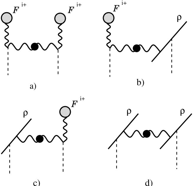
FIG. 1.: Feynman diagrams for the four contributions to $\chi$ given in eq. (48).

To the same accuracy, the induced source $\langle\delta\rho\rangle$ involves only the terms in $\delta\rho$ of second order in the fluctuations :

$$\,\hat{\sigma}_{a}(\vec{x})\,\equiv\,\langle\delta\rho_{a}(x)\rangle\,\,=\,\langle\delta\rho_{a}^{(2)}(x)\rangle,$$ (49)

with $\delta\rho_{a}^{(2)}$ given by eq. (41). This yields

$$\alpha_{s}\ln{1\over b}\,\sigma_{a}({\bf x}_{\perp})\,=\,\int dx^{-}\,{\rm Tr}\,(T^{a}\hat{\sigma}(\vec{x})),$$ (50)

where:

$$\hat{\sigma}(\vec{x}) \equiv -g\partial^{+}_{y}G^{ii}(x,y)\Big{|}_{x=y}\,+\,ig^{2}\rho({\vec{x}})\Bigl{\langle}x\bigg{|}{1\over i\partial^{-}}\,G^{--}{1\over i\partial^{-}}\bigg{|}x\Bigr{\rangle}$$ (51)

$$\equiv \hat{\sigma}_{1}(\vec{x})\,+\,\hat{\sigma}_{2}(\vec{x}).$$ (52)

In writing $\hat{\sigma}_{2}$ as above, we have used compact but formal notations for the second contribution to $\delta\rho_{a}^{(2)}$ in eq. (41), which is non-local in time. Diagramatically, the two terms in eq. (51) are represented by the one-loop diagrams displayed in Fig. 2. These are vertex and self-energy corrections which in the weak field limit (i.e., to linear order in $\rho$) generate the virtual piece of the BFKL kernel [13, 11]. Accordingly, we shall refer to $\sigma$ or $\hat{\sigma}$ as the virtual correction.

FIG. 2.: Feynman diagrams for $\hat{\sigma}_{1}$ (a) and $\hat{\sigma}_{2}$ (b,c,d). The wavy line with a blob denotes the background field propagator of the semi-fast gluons; the continuous line represents the source $\rho$; the precise vertices can be read off eq. (41).

II The induced charge-charge correlator, or “real correction”

We are now prepared for the explicit calculation of the coefficients in the RGE, to be completed in this and the following section. The one-loop quantum calculation will be performed fully in the LC-gauge ($a^{+}_{c}={\cal A}^{+}_{c}=0$), by using the retarded $i\epsilon$ prescription discussed in Sect. I C. The corresponding background field propagator is given explicitly in Appendix A. The ensuing expressions for $\chi$ and $\sigma$, which are gauge-covariant functionals of the background fields, will be then rotated to the COV-gauge for the background fields (cf. eq. (I B)), which is the only gauge which allows for explicit non-linear calculations.

In particular, the calculation of the “real correction” in this section will be organized as follows: We shall first compute $\hat{\chi}(\vec{x},\vec{y})$ by evaluating the matrix elements in the r.h.s. of eq. (48), then we shall derive $\chi({x}_{\perp},{y}_{\perp})$ by integrating out the longitudinal structure of $\hat{\chi}(\vec{x},\vec{y})$, cf. eq. (46). The result will be subsequently rotated to the (background) COV-gauge, to give $\tilde{\chi}({x}_{\perp},{y}_{\perp})$, cf. eq. (I B). Finally, the coefficient $\eta(x_{\perp},y_{\perp})$ in the RGE for $W_{\tau}[\alpha]$ will be obtained according to eq. (32).

A Non-linear effects and their dependence upon the gauge-fixing prescription

By substituting the expressions (A 4) for the gluon propagator in eq. (48) for $\hat{\chi}(\vec{x},\vec{y})$, one obtains, after simple algebra,

$${1\over g^{2}}{\hat{\chi}}(\vec{x},\vec{y}) = i2{\cal F}^{+i}_{x}\,\acute{G}^{ij}(x,y)\,2{\cal F}^{+j}_{y}$$ (55)

$$+(2{\cal F}^{+i}{\cal D}^{i}+\rho)_{x}{1\over i\partial^{+}}{\acute{G}}^{+j}(2{\cal F}^{+j})_{y}-(2{\cal F}^{+i})_{x}{\acute{G}}^{i+}{1\over i\partial^{+}}(2{\cal D}^{\dagger j}{\cal F}^{+j}+\rho)_{y}$$

$$+i\,(2{\cal F}^{+i}{\cal D}^{i}+\rho)_{x}{1\over i\partial^{+}}{\acute{G}}^{++}{1\over i\partial^{+}}(2{\cal D}^{\dagger j}{\cal F}^{+j}+\rho)_{y}$$

$$\equiv {1\over g^{2}}\Bigl{(}{\hat{\chi}}_{1}(\vec{x},\vec{y})\,+\,{\hat{\chi}}_{2}(\vec{x},\vec{y})\,+\,{\hat{\chi}}_{3}(\vec{x},\vec{y})\Bigr{)},$$ (56)

where the equal-time limit $y^{+}=x^{+}+\epsilon$ is implicit, and ${\hat{\chi}}_{1}$, ${\hat{\chi}}_{2}$, and ${\hat{\chi}}_{3}$ refer, respectively, to the terms in the first, second and third line.

In these expressions, ${\cal D}^{i}\equiv\partial^{i}-ig{\cal A}^{i}$ and ${\cal D}^{\dagger j}=\partial^{\dagger j}+ig{\cal A}^{j}$ (with the derivative $\partial^{\dagger j}$ acting on the function on its left) are covariant derivatives constructed with the background field ${\cal A}^{i}$. Furthermore, $\acute{G}^{\mu\nu}_{ab}(x,y)$ is the gluon propagator in the temporal gauge $\acute{a}^{-}_{c}=0$, and is presented in Appendix A.3. It is a non-linear functional of the background field $\alpha(\vec{x})$, via the Wilson lines $V$ and $V^{\dagger}$ (see, e.g., eqs. (A15)–(A17)). What is however remarkable, and will be demonstrated in what follows, is that all the non-linear effects encoded in $\acute{G}^{\mu\nu}$ drop out in the calculation of the matrix elements in eq. (55). That is, the final result for $\hat{\chi}(\vec{x},\vec{y})$ is the same as obtained by evaluating the r.h.s. of eq. (55) with the free temporal-gauge propagator $\acute{G}^{\mu\nu}_{0}$. This simplification is a consequence of our specific $i\epsilon$ prescription in the LC-gauge propagator, as we explain now. Consider the following matrix element:

$$\langle x|{1\over i\partial^{+}}{\acute{G}}^{++}{1\over i\partial^{+}}|y\rangle$$ (57)

which enters the r.h.s. of eq. (55). Our “retarded” prescription in $G^{\mu\nu}$ implies that, on the left of ${\acute{G}}^{++}$ in eq. (57), ${1\over i\partial^{+}}\equiv{1\over i\partial^{+}+i\epsilon}$ should be retarded, while on the right ${1\over i\partial^{+}}\equiv{1\over i\partial^{+}-i\epsilon}$ should rather be advanced (cf. eqs. (A25)–(A 4)). Thus, eq. (57) is the same as

$$\int dz_{1}^{-}\,\int dz_{2}^{-}\,\langle x^{-}|{1\over i\partial^{+}+i\epsilon}|z_{1}^{-}\rangle\,\langle x^{+},z_{1}^{-},x_{\perp}|\ {\acute{G}}^{++}\ |y^{+},z_{2}^{-},y_{\perp}\rangle\,\langle z_{2}^{-}|{1\over i\partial^{+}-i\epsilon}|y^{-}\rangle$$ (58)

$$=\int dz_{1}^{-}\,\int dz_{2}^{-}\,\theta(x^{-}-z_{1}^{-})\ {\acute{G}}^{++}(z_{1}^{-},z_{2}^{-})\ \theta(y^{-}-z_{2}^{-})\ ,$$ (59)

where in the second line only the longitudinal coordinates have been shown explicitly. In eq. (55), this matrix element is sandwiched between $\rho(\vec{x})$ and $\rho(\vec{y})$. Since $\rho(\vec{x})$ is localized at small$x^{-}$ ($x^{-}\mathrel{\hbox to0.0pt{\raise 2.20013pt\hbox{$<$}\hss}{\lower 2.20013pt\hbox{$\sim$}}}x^{-}_{\tau}$, cf. eq. (23)), while $G^{\mu\nu}(x,y)$ is relatively slowly varying as a function of $x^{-}$ and $y^{-}$ (since this is the propagator of the semi-fast gluons, with $p^{+}\ll\Lambda^{+}$), one can effectively replace $x^{-}\simeq 0$ and $y^{-}\simeq 0$ in eq. (58) [and everywhere else in eq. (55); recall that the electric field ${\cal F}^{+i}$ is as localized as $\rho$]. This gives, for $x^{+}=y^{+}$,

$$\langle x^{-}\simeq 0,\,x_{\perp}|{1\over i\partial^{+}}{\acute{G}}^{++}{1\over i\partial^{+}}\,|y^{-}\simeq 0,\,y_{\perp}\rangle=\int dz_{1}^{-}\int dz_{2}^{-}\,\theta(-z_{1}^{-}){\acute{G}}^{++}(z_{1}^{-},z_{2}^{-})\theta(-z_{2}^{-})\ ,$$ (60)

which shows that both external points $z_{1}^{-},z_{2}^{-}$ in ${\acute{G}}$ are negative, so ${\acute{G}}$ must be non-crossing. (Recall that “crossing” and “non-crossing” refer to whether the gluon has propagated or not accross the surface at $x^{-}=0$, where the color source is located; see Sect. 6 of Paper I and Appendix A in this paper.) Moreover, the non-crossing piece of ${\acute{G}(z_{1}^{-},z_{2}^{-})}$ at negative $z_{1}^{-},z_{2}^{-}$ is the same as the corresponding piece of the free propagator. Thus, the matrix element (60) singles out that particular piece of ${\acute{G}}$ which is not affected by the background field.

A similar conclusion applies to the other terms in the r.h.s. of eq. (55), which involve the following matrix elements

$$\langle x|\acute{G}^{ij}|y\rangle,\qquad\langle x|{1\over i\partial^{+}}{\acute{G}}^{+i}|y\rangle,\qquad\langle x|{\acute{G}}^{i+}{1\over i\partial^{+}}|y\rangle,$$ (61)

evaluated at $x^{-}\simeq y^{-}\simeq 0$ and $y^{+}=x^{+}+\epsilon$. For instance, in the first term above, one can use the continuity of ${\acute{G}}^{ij}$ at $x^{-}=0$ and $y^{-}=0$ (cf. Appendix A) to approach these points from $x^{-}<0$ and $y^{-}<0$, i.e., from the domain where ${\acute{G}}^{ij}$ coincides with the corresponding free propagator ${\acute{G}}^{ij}_{0}$. We thus deduce that

$$\langle 0,x_{\perp}|\acute{G}^{ij}|0,y_{\perp}\rangle=\langle 0,x_{\perp}|\acute{G}_{0}^{ij}|0,y_{\perp}\rangle\,,$$ (62)

and similarly for the other matrix elements in eq. (61).

For the previous arguments, it has been essential that the retarded prescription has been used systematically in the LC-gauge, both in the classical solution and in the quantum propagator: (a) The retarded boundary condition on the classical solution has insured that the background field ${\cal A}^{i}$ is non-vanishing only at $x^{-}>0$, or $z<t$. That is, the classical field sits behind its source, the (fast degrees of freedom of the) hadron, which is located at $z=t$. (b) The retarded $i\epsilon$ prescription in the gluon propagator has implied that the semi-fast gluon exchanged within $\hat{\chi}$ (cf. Fig. 1) is confined at negative $x^{-}$, where there is no background field. Thus, this quantum gluon propagates freely from $\vec{y}$ to $\vec{x}$, with $x^{-}\simeq y^{-}\simeq 0$.

Note, however, that this property of a free propagation holds only for the temporal gauge gluon $\acute{a}^{\mu}$ (with $\acute{a}^{-}=0$), which does not couple directly to the singular color source $\rho$ [11]. Because of that, its propagator $\acute{G}^{\mu\nu}(x,y)$ is continuous at $x^{-}=0$ and $y^{-}=0$, and the associated non-linear effects drop out in the calculation of $\hat{\chi}$, as argued before. By contrast, the light-cone gauge propagator $G^{\mu\nu}(x,y)$ is sensitive also to the discontinuous gauge rotations at the end points $x^{-}$ and $y^{-}$, via the covariant derivatives ${\cal D}^{i}_{x}$ and ${\cal D}^{\dagger j}_{y}$ (which technically enter via the gauge rotation from the temporal gauge to the LC gauge; cf. eq. (A19)). As obvious on eq. (55), the non-linear effects associated with the fields within ${\cal D}^{i}_{x}$ and ${\cal D}^{\dagger j}_{y}$ do subsist in the final result for $\hat{\chi}$. Thus, while it is correct to replace the temporal gauge propagator $\acute{G}^{\mu\nu}$ in eq. (55) by its free counterpart, such a replacement would not be legitimate for the light-cone gauge propagator $G^{\mu\nu}$ in eq. (48).

By inspection of the previous arguments, it should be also clear that they would still hold, mutas mutandis, after replacing everywhere the retarded prescription with an advanced one: The corresponding classical field ${\cal A}^{i}$ would have support only at negative $x^{-}$, while the semi-fast gluon exchanged within $\hat{\chi}$ would freely propagate at positive $x^{-}$.

In Refs. [2, 14, 16], where the advanced prescription has been used extensively, one has found similar simplifications in the calculation of Feynman graphs for, e.g., the scattering of a quark or a gluon off a hadronic target. As shown there, it is only with this prescription that one can ignore the final state interactions of the struck quark (or gluon) in deep inelastic scattering, which is essential if the produced jet is to be used as an indicator of the hadron wavefunction. Our present analysis corroborates the conclusions in Refs. [2, 14, 16] that retarded and advanced LC-gauge prescriptions are special in that they not only lead to technical simplifications, but also allow for a more transparent physical interpretation of the results. With more symmetrical prescriptions like principal value PV$\,1\over p^{+}$ or Leibbrandt-Mandelstam, one cannot avoid the overlap between the classical fields and the quantum fluctuations, and thus neither the final/initial state interactions.

To summarize, when computing ${\hat{\chi}}$ with a retarded prescription, one can replace ${\acute{G}}^{\mu\nu}$ in eq. (55) by the corresponding free propagator ${\acute{G}}^{\mu\nu}_{0}$. This calculation will be presented in the following subsection. For completness, in Appendix B we shall verify, on the example of $\hat{\chi}_{3}$, that a lengthier calculation using the full propagator ${\acute{G}}^{\mu\nu}$ leads eventually to the same result.

B Explicit calculation of $\hat{\chi}(\vec{x},\vec{y})$

With ${\acute{G}}^{ij}$ replaced by the free propagator ${\acute{G}}^{ij}_{0}=\delta^{ij}G_{0}$ the first term ${\hat{\chi}}_{1}$ in the r.h.s. of eq. (55) has been already computed in Sect. 5.2 of Paper I, with the following result:

$${\hat{\chi}}_{1}={g^{2}\over\pi}\ln(1/b)\ {\cal F}^{+i}_{x}\ {\cal F}^{+j}_{y}\ \int{d^{2}p_{\perp}\over(2\pi)^{2}}\,{\rm e}^{ip_{\perp}\cdot(x_{\perp}-y_{\perp})}\,.$$ (63)

Consider now the matrix element (57) which enters ${\hat{\chi}}_{3}$. With ${\acute{G}}^{++}\rightarrow{\acute{G}}^{++}_{0}$, cf. eq. (A18), this gives (for $y^{+}=x^{+}$, and $x^{-}\simeq y^{-}\simeq 0$)

$$\langle 0,x_{\perp}|{1\over i\partial^{+}+i\epsilon}\,{\acute{G}}^{++}_{0}{1\over i\partial^{+}-i\epsilon}|0,y_{\perp}\rangle\,=\,\qquad\qquad\qquad$$ (64)

$$\,=\,\int_{strip}{dp^{-}\over 2\pi}\int{dp^{+}\over 2\pi}\int{d^{2}p_{\perp}\over(2\pi)^{2}}\,{\rm e}^{ip_{\perp}\cdot(x_{\perp}-y_{\perp})}\,{1\over p^{+}+i\epsilon}\,{2p^{+}\over p^{-}}\,G_{0}(p)\,{1\over p^{+}-i\epsilon}\,,$$ (65)

where the integral over $p^{-}$ is restricted to the strip (45). The various factors of $p^{+}$ in the integrand can be combined into a PV prescription in $1/p^{+}$ :

$${2p^{+}\over(p^{+}+i\epsilon)(p^{+}-i\epsilon)}\,=\,{1\over p^{+}+i\epsilon}\,+\,{1\over p^{+}-i\epsilon}\,=\,2{\rm PV}\,{1\over p^{+}}\,.$$ (66)

Then, the integral over $p^{+}$ is easily computed by contour techniques:

$$\int{dp^{+}\over 2\pi}\,{\rm PV}\,{1\over p^{+}}\,{1\over 2p^{+}p^{-}-p_{\perp}^{2}+i\epsilon}\,=\,{-i\epsilon(p^{-})\over 2p_{\perp}^{2}}\,,$$ (67)

where $\epsilon(p^{-})\equiv\theta(p^{-})-\theta(-p^{-})$ is the sign function. The restricted integral over $p^{-}$ generates the expected logarithmic enhancement (below, $\Lambda\equiv\Lambda^{-}$, cf. eq. (45)) :

$$\int_{strip}{dp^{-}\over 2\pi}\,\,{\epsilon(p^{-})\over p^{-}}\,\equiv\,\left(\int_{-\Lambda/b}^{-\Lambda}+\int_{\Lambda}^{\Lambda/b}\right){dp^{-}\over 2\pi}\,{\epsilon(p^{-})\over p^{-}}\,=\,{1\over\pi}\,\ln(1/b)\,.$$ (68)

The final result reads

$$\langle 0,x_{\perp}|{1\over i\partial^{+}+i\epsilon}\,{\acute{G}}^{++}{1\over i\partial^{+}-i\epsilon}|0,y_{\perp}\rangle\,=\,{-i\over\pi}\ln(1/b)\,\int{d^{2}p_{\perp}\over(2\pi)^{2}}\,{1\over p_{\perp}^{2}}\,{\rm e}^{ip_{\perp}\cdot(x_{\perp}-y_{\perp})}\,,$$ (69)

which immediately implies:

$${\hat{\chi}}_{3}={g^{2}\over\pi}\ln(1/b)\ \int{d^{2}p_{\perp}\over(2\pi)^{2}}\,{1\over p_{\perp}^{2}}\ (2{\cal F}^{+i}{\cal D}^{i}+\rho)_{x}\ {\rm e}^{ip_{\perp}\cdot(x_{\perp}-y_{\perp})}\ (2{\cal D}^{\dagger j}{\cal F}^{+j}+\rho)_{y}\ .$$ (70)

A similar calculation yields:

$$\langle 0,x_{\perp}|{1\over i\partial^{+}+i\epsilon}\,{\acute{G}}^{+i}|0,y_{\perp}\rangle = \langle 0,x_{\perp}|{\acute{G}}^{i+}{1\over i\partial^{+}-i\epsilon}|0,y_{\perp}\rangle\,$$ (71)

$$= {-i\over 2\pi}\ln(1/b)\int{d^{2}p_{\perp}\over(2\pi)^{2}}\,{p^{i}\over p_{\perp}^{2}}\,{\rm e}^{ip_{\perp}\cdot(x_{\perp}-y_{\perp})}\,,$$ (72)

which allows us to also compute ${\hat{\chi}}_{2}$ :

$${\hat{\chi}}_{2}={-g^{2}\over\pi}\ln(1/b)\int{d^{2}p_{\perp}\over(2\pi)^{2}}\,{1\over p_{\perp}^{2}}\ \biggl{\{}(2{\cal F}^{+i}{\cal D}^{i}+\rho)_{x}\ {\rm e}^{ip_{\perp}\cdot(x_{\perp}-y_{\perp})}\ (2\partial^{\dagger j}{\cal F}^{+j})_{y}\,+\,$$ (73)

$$\,\,\,\,+\,(2{\cal F}^{+i}\partial^{i})_{x}\ {\rm e}^{ip_{\perp}\cdot(x_{\perp}-y_{\perp})}\ (2{\cal D}^{\dagger j}{\cal F}^{+j}+\rho)_{y}\biggr{\}}$$ (74)

The previous results for ${\hat{\chi}}_{1}$, ${\hat{\chi}}_{2}$, and ${\hat{\chi}}_{3}$ are conveniently combined as:

$${\hat{\chi}}(\vec{x},\vec{y}) = {g^{2}\over\pi}\ln{1\over b}\,\Biggl{\{}{\cal F}^{+i}_{x}\,\delta^{ij}_{\perp}(x_{\perp}-y_{\perp})\,{\cal F}^{+j}_{y}\,+\,$$ (76)

$$\qquad\,\,\,\,+\,\biggl{[}2{\cal F}^{+i}\biggl{(}{\cal D}^{i}-{\partial^{i}\over 2}\biggr{)}+\rho\biggr{]}_{x}\,\langle x_{\perp}|{1\over-\nabla_{\perp}^{2}}|y_{\perp}\rangle\,\biggl{[}2\biggl{(}{\cal D}^{\dagger j}-{\partial^{\dagger j}\over 2}\biggr{)}{\cal F}^{+j}+\rho\biggr{]}_{y}\Biggr{\}}\ ,$$

which is our final expression for ${\hat{\chi}}$. The following notations have been used:

$$\delta^{ij}_{\perp}(x_{\perp}-y_{\perp}) = \int{d^{2}p_{\perp}\over(2\pi)^{2}}\,\left(\delta^{ij}-{p^{i}p^{j}\over p_{\perp}^{2}}\right)\ {\rm e}^{ip_{\perp}\cdot(x_{\perp}-y_{\perp})}\,,$$ (77)

$$\langle x_{\perp}|{1\over-\nabla_{\perp}^{2}}|y_{\perp}\rangle = \int{d^{2}p_{\perp}\over(2\pi)^{2}}\,{1\over p_{\perp}^{2}}\ {\rm e}^{ip_{\perp}\cdot(x_{\perp}-y_{\perp})}\,.$$ (78)

C The two-dimensional correlator $\chi(x_{\perp},y_{\perp})$

In eq. (76), both $\rho$ and ${\cal F}^{+i}$ have support near the LC, at $x^{-}\mathrel{\hbox to0.0pt{\raise 2.20013pt\hbox{$<$}\hss}{\lower 2.20013pt\hbox{$\sim$}}}x^{-}_{\tau}\equiv 1/\Lambda^{+}$. Thus, although induced by quantum modes with relatively large longitudinal wavelengths $\Delta x^{-}\gg 1/\Lambda^{+}$, the charge-charge correlator appears to be as localized in the longitudinal direction as the original source at the scale $\Lambda^{+}$. This is so because the vertices responsible for this quantum effect are explicitly proportional to $\rho$ or ${\cal F}^{+i}$ (cf. eq. (36)). Thus, $\hat{\chi}(\vec{x},\vec{y})$ is manifestly sensitive to the internal structure of the source, and also to the structure of the background field at small distances $x^{-}\mathrel{\hbox to0.0pt{\raise 2.20013pt\hbox{$<$}\hss}{\lower 2.20013pt\hbox{$\sim$}}}x^{-}_{\tau}$. (Note, in particular, that eq. (76) involves the product ${\cal F}^{+i}(\vec{x}){\cal A}^{i}(\vec{x})$, and thus the field ${\cal A}^{i}(\vec{x})$ within the support of $\rho$.)

If this was also true for the two-dimensional density $\chi(x_{\perp},y_{\perp})$, which is the quantity which enters the RGE (19), this would spoil the separation of scales assumed by the effective theory, and thus the validity of the latter. Note that, the simple fact that $\chi(x_{\perp},y_{\perp})$ is obtained from $\hat{\chi}(\vec{x},\vec{y})$ after integrating out $x^{-}$ and $y^{-}$, cf. eq. (46), is by itself not sufficient to guarantee that the physical information about small $x^{-}$ or $y^{-}$ is truly irrelevant. For instance, the following integrated quantity

$$\int dx^{-}{\cal F}^{+i}(\vec{x}){\cal A}^{i}(\vec{x}),$$ (79)

although a function of $x_{\perp}$ alone, is nevertheless sensitive to the values of ${\cal A}^{i}(\vec{x})$ at $x^{-}\mathrel{\hbox to0.0pt{\raise 2.20013pt\hbox{$<$}\hss}{\lower 2.20013pt\hbox{$\sim$}}}x^{-}_{\tau}$, since the electric field ${\cal F}^{+i}(\vec{x})$ has its support there (cf. eq. (10)). On the other hand, the following quantity (recall that ${\cal A}^{i}(x^{-}\to\infty)={\cal A}^{i}_{\infty}$, while ${\cal A}^{i}(x^{-}\to-\infty)=0$)

$$\int dx^{-}{\cal F}^{+i}(\vec{x})\,=\,\int dx^{-}\partial^{+}{\cal A}^{i}\,=\,{\cal A}^{i}_{\infty}(x_{\perp})$$ (80)

is not sensitive to the structure of ${\cal A}^{i}(\vec{x})$ around the origin, but only to its asymptotic value at large $x^{-}$.

As we shall demonstrate now, this latter situation applies also to $\hat{\chi}(\vec{x},\vec{y})$, which, like the electric field ${\cal F}^{+i}(\vec{x})$, is a total derivative with respect to its longitudinal arguments $x^{-}$ and $y^{-}$:

$${\hat{\chi}}(\vec{x},\vec{y})=\partial^{+}_{x}\partial^{+}_{y}\ {\cal C}(\vec{x},\vec{y})\ .$$ (81)

To see this, note the following identities, which hold for an arbitrary function $\Phi(x_{\perp})$,

$$(2{\cal F}^{+i}{\cal D}^{i}+\rho)_{x}\ \Phi(x_{\perp}) = i\partial^{+}_{x}{\cal D}^{2}_{x}\Phi(x_{\perp}),$$ (82)

$$\Phi(y_{\perp})(2{\cal D}^{\dagger j}{\cal F}^{+j}+\rho)_{y} = -i\Phi(y_{\perp}){\cal D}^{\dagger 2}_{y}\partial^{+}_{y}\,$$ (83)

(with $\partial^{+}_{y}$ in the second line acting on the function on its left). These identities rely on the classical equation of motion (3), that is,

$$\partial^{i}{\cal F}^{+i}-ig[{\cal A}^{i},{\cal F}^{+i}]=\rho\,.$$ (84)

For instance, one can obtain the first identity by writing:

$$\partial^{+}{\cal D}^{2}\Phi(x_{\perp}) = \partial^{+}\Bigl{(}(\partial^{i}-ig{\cal A}^{i})(\partial^{i}\Phi-ig{\cal A}^{i}\Phi)\Bigr{)}$$ (85)

$$= -i({\cal F}^{+i}\Phi)-i{\cal F}^{+i}\partial^{i}\Phi-ig({\cal F}^{+i}{\cal A}^{i}+{\cal A}^{i}{\cal F}^{+i})\Phi$$ (86)

$$= -i\Bigl{\{}\partial^{i}{\cal F}^{+i}+ig({\cal F}^{+i}{\cal A}^{i}-{\cal A}^{i}{\cal F}^{+i})+2{\cal F}^{+i}{\cal D}^{i}\Bigr{\}}\Phi$$ (87)

$$= -i(\rho+2{\cal F}^{+i}{\cal D}^{i})\Phi\,$$ (88)

where in writing the second line we have used $\partial^{+}\Phi=0$ and $\partial^{+}{\cal A}^{i}={\cal F}^{+i}$, and the last line follows from the previous one after using (84).

By using eqs. (82) and (76), one deduces that $\hat{\chi}(\vec{x},\vec{y})$ is indeed of the total-derivative form (81), with

$${\cal C}(\vec{x},\vec{y})\,=\,{g^{2}\over\pi}\ln{1\over b}\ \left\{{\cal A}^{i}_{x}\ \delta^{ij}_{\perp}(x_{\perp}-y_{\perp})\ {\cal A}^{j}_{y}+({\cal D}^{i}{\cal A}^{i})_{x}\langle x_{\perp}|{1\over-\nabla_{\perp}^{2}}|y_{\perp}\rangle({\cal A}^{j}{\cal D}^{\dagger j})_{y}\right\}\ .$$ (89)

Then, the integrations over $x^{-}$ and $y^{-}$ in eq. (46) become trivial, and yield

$${\chi}(x_{\perp},y_{\perp})=4\biggl{\{}{\cal A}^{i}_{\infty}(x_{\perp})\ \delta^{ij}_{\perp}(x_{\perp}-y_{\perp}){\cal A}^{j}_{\infty}(y_{\perp})+({\cal D}^{i}_{\infty}{\cal A}^{i}_{\infty})_{x_{\perp}}\langle x_{\perp}|{1\over-\nabla_{\perp}^{2}}|y_{\perp}\rangle({\cal A}^{j}_{\infty}{\cal D}^{\dagger j}_{\infty})_{y_{\perp}}\biggr{\}}$$ (90)

(with ${\cal D}^{i}_{\infty}\equiv\partial^{i}-ig{\cal A}^{i}_{\infty}(x_{\perp})$) which is sensitive only to the asymptotic fields.

The gauge rotation (I B) of eq. (90) to the background COV-gauge is straightforward. By using ${\cal A}^{i}_{\infty}(x_{\perp})=(i/g)V_{x}\partial^{i}V^{\dagger}_{x}$ (cf. eq. (9)), one immediately finds

$$\tilde{\chi}(x_{\perp},y_{\perp})\,=\,{4\over g^{2}}\,\biggl{\{}\partial^{i}V^{\dagger}_{x}\,\delta^{ij}_{\perp}(x_{\perp}-y_{\perp})\partial^{j}V_{y}\,+\,\partial^{i}_{x}\biggl{(}\Bigl{(}\partial^{i}V^{\dagger}\Bigr{)}_{x}\langle x_{\perp}|\,{1\over-\nabla^{2}_{\perp}}\,|y_{\perp}\rangle\Bigl{(}\partial^{j}V\Bigr{)}_{y}\biggr{)}\partial^{\dagger j}_{y}\biggr{\}},\,\,$$ (91)

where $V^{\dagger}_{x}\equiv V^{\dagger}(x_{\perp})$, cf. eq. (11), and the derivatives not included in the brackets act on all the functions on their right (or left).

D From $\chi$ to $\eta$

Eq. (91) provides $\tilde{\chi}(x_{\perp},y_{\perp})$ as an explicit functional of the field $\alpha(\vec{x})$, via the asymptotic Wilson lines $V(x_{\perp})$ and $V^{\dagger}(x_{\perp})$. It is therefore more convenient to write down the evolution equation in terms of $\alpha$ rather than ${\tilde{\rho}}$. The appropriate transformation $\tilde{\chi}\rightarrow\eta$ is shown in eq. (32), and will be worked out in detail in what follows.

We shall do that in two steps, corresponding to the two terms in the r.h.s. of eq. (91), which we write as $\tilde{\chi}=\tilde{\chi}_{1}+\tilde{\chi}_{2}$. Correspondingly, $\eta=\eta_{1}+\eta_{2}$ with (we omit the factor of $4/g^{2}$ at intermediate steps)

$$\eta_{1}(x_{\perp},y_{\perp}) \equiv \int d^{2}z_{\perp}\int d^{2}u_{\perp}\langle x_{\perp}|{1\over-\nabla^{2}_{\perp}}\,|z_{\perp}\rangle\,\Bigl{(}\partial^{i}_{z}\partial^{j}_{u}\left\{V^{\dagger}_{z}\delta^{ij}_{\perp}(z_{\perp}-u_{\perp})V_{u}\right\}\Bigr{)}\langle u_{\perp}|{1\over-\nabla^{2}_{\perp}}|y_{\perp}\rangle$$ (92)

$$= -\int d^{2}z_{\perp}\int d^{2}u_{\perp}\langle x_{\perp}|{\partial^{i}\over-\nabla^{2}_{\perp}}|z_{\perp}\rangle\,V^{\dagger}_{z}\,\langle z_{\perp}|\delta^{ij}-{\partial^{i}\partial^{j}\over\nabla^{2}_{\perp}}\,|u_{\perp}\rangle\,V_{u}\,\langle u_{\perp}|{\partial^{j}\over-\nabla^{2}_{\perp}}|y_{\perp}\rangle,$$ (93)

where the second line follows after some integrations by parts, and we have written

$$\langle x_{\perp}|\,{\partial^{i}\over-\nabla^{2}_{\perp}}\,|y_{\perp}\rangle\,\equiv\,\partial^{i}_{x}\,\langle x_{\perp}|\,{1\over-\nabla^{2}_{\perp}}\,|y_{\perp}\rangle\,=\int{d^{2}p_{\perp}\over(2\pi)^{2}}\,{-i\,p^{i}\over p_{\perp}^{2}}\,{\rm e}^{ip_{\perp}\cdot(x_{\perp}-y_{\perp})}\,.$$ (94)

Similarly,

$$\eta_{2}(x_{\perp},y_{\perp}) = -\int d^{2}z_{\perp}\int d^{2}u_{\perp}\langle x_{\perp}|{\partial^{i}\over-\nabla^{2}_{\perp}}|z_{\perp}\rangle(\partial^{i}V^{\dagger}_{z})\langle z_{\perp}|{1\over-\nabla^{2}_{\perp}}|u_{\perp}\rangle(\partial^{j}V_{u})\langle u_{\perp}|{\partial^{j}\over-\nabla^{2}_{\perp}}|y_{\perp}\rangle$$ (95)

$$= -\int d^{2}z_{\perp}\int d^{2}u_{\perp}V^{\dagger}_{z}V_{u}\,\partial^{i}_{z}\partial^{j}_{u}\langle x_{\perp}|{\partial^{i}\over-\nabla^{2}_{\perp}}|z_{\perp}\rangle\langle z_{\perp}|{1\over-\nabla^{2}_{\perp}}|u_{\perp}\rangle\langle u_{\perp}|{\partial^{j}\over-\nabla^{2}_{\perp}}|y_{\perp}\rangle.$$ (96)

By using

$$\partial^{i}_{x}\langle x_{\perp}|\,{\partial^{i}\over-\nabla^{2}_{\perp}}\,|y_{\perp}\rangle\,=\,-\delta^{(2)}(x_{\perp}-y_{\perp}),$$ (97)

this can be further transformed as

$$\eta_{2}(x_{\perp},y_{\perp}) = V^{\dagger}_{x}\,\langle x_{\perp}|\,{1\over-\nabla^{2}_{\perp}}\,|y_{\perp}\rangle\,V_{y}\,$$ (101)

$$\,\,+\,\int d^{2}u_{\perp}\,V^{\dagger}_{x}\,\langle x_{\perp}|\,{\partial^{j}\over-\nabla^{2}_{\perp}}\,|u_{\perp}\rangle\,V_{u}\,\langle u_{\perp}|\,{\partial^{j}\over-\nabla^{2}_{\perp}}\,|y_{\perp}\rangle\,$$

$$\,\,+\int d^{2}z_{\perp}\,\langle x_{\perp}|\,{\partial^{i}\over-\nabla^{2}_{\perp}}\,|z_{\perp}\rangle\,V^{\dagger}_{z}\,\langle z_{\perp}|\,{\partial^{i}\over-\nabla^{2}_{\perp}}\,|y_{\perp}\rangle\,V_{y}\,$$

$$\,\,+\int d^{2}u_{\perp}\,\int d^{2}z_{\perp}\,\langle x_{\perp}|\,{\partial^{i}\over-\nabla^{2}_{\perp}}\,|z_{\perp}\rangle\,V^{\dagger}_{z}\,\langle z_{\perp}|\,{\partial^{i}\partial^{j}\over-\nabla^{2}_{\perp}}\,|u_{\perp}\rangle\,V_{u}\langle u_{\perp}|\,{\partial^{j}\over-\nabla^{2}_{\perp}}\,|y_{\perp}\rangle\,.$$

The last term in the above expression is non-local in both $u$ and $z$, but it cancels against the similar term that contributes to $\eta_{1}$, eq. (92). So we arrive at

$$\eta(x_{\perp},y_{\perp}) = (1\,+\,V^{\dagger}_{x}V_{y})\,\langle x_{\perp}|\,{1\over-\nabla^{2}_{\perp}}\,|y_{\perp}\rangle\,$$ (103)

$$\,+\,\int d^{2}z_{\perp}\,\langle x_{\perp}|\,{\partial^{i}\over-\nabla^{2}_{\perp}}\,|z_{\perp}\rangle\,\langle z_{\perp}|\,{\partial^{i}\over-\nabla^{2}_{\perp}}\,|y_{\perp}\rangle\,(V^{\dagger}_{x}V_{z}\,+\,V^{\dagger}_{z}V_{y})\,.$$

By also using

$$\int d^{2}z_{\perp}\,\langle x_{\perp}|\,{\partial^{i}\over-\nabla^{2}_{\perp}}\,|z_{\perp}\rangle\,\langle z_{\perp}|\,{\partial^{i}\over-\nabla^{2}_{\perp}}\,|y_{\perp}\rangle\,=\,-\langle x_{\perp}|\,{1\over-\nabla^{2}_{\perp}}\,|y_{\perp}\rangle\,$$ (104)

we finally express $\eta$ as (below, we reintroduce the overall factor $4/g^{2}$)

$$\eta_{ab}(x_{\perp},y_{\perp})\,=\,{4\over g^{2}}\int{d^{2}z_{\perp}\over(2\pi)^{2}}\,{(x^{i}-z^{i})(y^{i}-z^{i})\over(x_{\perp}-z_{\perp})^{2}(y_{\perp}-z_{\perp})^{2}}\Bigl{\{}1+V^{\dagger}_{x}V_{y}-V^{\dagger}_{x}V_{z}-V^{\dagger}_{z}V_{y}\Bigr{\}}_{ab}\,.$$ (105)

The kernel in this equation has been written in coordinate space by using eq. (94) and

$$\int{d^{2}p_{\perp}\over(2\pi)^{2}}\int{d^{2}k_{\perp}\over(2\pi)^{2}}\,\,{p_{\perp}\cdot k_{\perp}\over p_{\perp}^{2}k_{\perp}^{2}}\,\,{\rm e}^{ip_{\perp}\cdot(x_{\perp}-z_{\perp})}\,{\rm e}^{ik_{\perp}\cdot(z_{\perp}-y_{\perp})}\,=\,{1\over(2\pi)^{2}}\,{(x^{i}-z^{i})(y^{i}-z^{i})\over(x_{\perp}-z_{\perp})^{2}(y_{\perp}-z_{\perp})^{2}}\,.$$ (106)

Eq. (105) is our final result for the “real correction”, to which we shall return in Sect. IV A.

III The induced color charge, of “virtual correction”

We shall now similarly compute the coefficient $\nu$ in the RGE (29), or the “virtual correction”. This calculation will be organized as follows: By evaluating the r.h.s. of eq. (51), we shall first obtain the three-dimensional color charge density $\hat{\sigma}(\vec{x})$ in the LC gauge. The longitudinal structure of the result will be explored, and then integrated out, to yield the two-dimensional density $\sigma_{a}({x}_{\perp})$, cf. eq. (50). In a separate calculation, based on eq. (91) for $\tilde{\chi}(x_{\perp},y_{\perp})$, we shall obtain the classical polarization $\delta\sigma({x}_{\perp})$ defined by eq. (28). By combining the various results as shown in eq. (27), we shall deduce the induced source $\tilde{\sigma}_{a}(x_{\perp})$ in the (background-field) COV-gauge, from which $\nu_{a}(x_{\perp})$ will be finally extracted, as shown in eq. (31).

At intermediate steps in this calculation we shall meet with logarithmic “tadpoles”, i.e., contributions to $\sigma$ or $\delta\sigma$ which are local in $x_{\perp}$ and proportional to

$$\int{d^{2}p_{\perp}\over p_{\perp}^{2}}\,.$$ (107)

Moreover, the momentum integrals giving the remaining, non-local, contributions will generally involve logarithmic ultraviolet (UV) divergences. After summing up the various contributions, all UV divergences must go away. Indeed, our one-loop calculation cannot introduce other UV divergences than those of the standard perturbation theory, which, moreover, must be absent as well, since they are not enhanced by the longitudinal logarithm $\ln(1/x)$. (In other terms, the UV divergent terms are purely ${\cal O}(\alpha_{s})$ effects, which are a priori ignored in our LLA.) To shorten the presentation, in this section we shall simply ignore all the tadpoles. At the very end, we shall verify that the final, non-local, result for $\tilde{\sigma}_{a}$ (or $\nu_{a}$) is UV finite, meaning that all the tadpoles must have cancelled among themselves.

The infrared finiteness, on the other hand, is a different issue, which, as in the corresponding BFKL problem, is related to subtle compensations between real and virtual corrections. We shall return to this issue in the discussion of the results in Sects. IV and V.

A Explicit calculation of $\hat{\sigma}(\vec{x})$

Eq. (51) shows that there are two contributions to the induced source: $\hat{\sigma}=\hat{\sigma}_{1}+\hat{\sigma}_{2}$. The second contribution $\hat{\sigma}_{2}$, to be computed in Appendix C, turns out to be a pure tadpole, and as such it will be ignored in what follows. The first contribution $\hat{\sigma}_{1}$, to be computed below, is given by:

$${\hat{\sigma}}_{1}^{a}(\vec{x})\,=\,{\rm Tr}\,(T^{a}\hat{\sigma}_{1}(\vec{x})),\qquad{\hat{\sigma}}_{1}(\vec{x})\,=\,-g\partial^{+}_{y}G^{ii}(x,y)\Big{|}_{x=y}\,.$$ (108)

It can be verified that, out of the four different terms in eq. (A21) for $G^{ij}$, it is only the last one, namely

$$G_{4}^{ii}(x,y) \equiv -\langle x|{\cal D}^{i}{1\over\partial^{+}}\,\acute{G}^{++}\,{1\over\partial^{+}}{\cal D}^{\dagger\,i}|y\rangle$$ (109)

$$= {\cal D}^{i}_{x}\int dz^{-}_{1}dz^{-}_{2}\langle x^{-}|{1\over i\partial^{+}+i\epsilon}|z^{-}_{1}\rangle{\acute{G}}^{++}(z^{-}_{1},x_{\perp};z^{-}_{2},y_{\perp})\langle z^{-}_{2}|{1\over i\partial^{+}-i\epsilon}|y^{-}\rangle{\cal D}^{\dagger\,i}_{y}\,,$$ (110)

that gives a non-vanishing contribution to $\hat{\sigma}_{1}$. The derivative $\partial^{+}_{y}$ in eq. (108) is readily performed as :

$$\partial^{+}_{y}\langle z^{-}_{2}|{1\over i\partial^{+}}|y^{-}\rangle\,\Big{(}\partial^{\dagger\,i}_{y}\,+ig{\cal A}^{i}(\vec{y})\Bigr{)}\,=\,i\delta(z^{-}_{2}-y^{-}){\cal D}^{\dagger\,i}_{y}\,+\,ig\langle z^{-}_{2}|{1\over i\partial^{+}}|y^{-}\rangle\,{\cal F}^{+i}(\vec{y})\,,$$ (111)

thus giving the following two contributions to $\hat{\sigma}_{1}$ :

$${\hat{\sigma}}_{1}(\vec{x})\,=\,-ig^{2}\langle x|{\cal D}^{i}{1\over i\partial^{+}}{\acute{G}}^{++}{1\over i\partial^{+}}|x\rangle\,{\cal F}^{+i}(\vec{x})\,-\,ig\langle x|{\cal D}^{i}{1\over i\partial^{+}}{\acute{G}}^{++}{\cal D}^{\dagger i}|x\rangle\,\equiv\,{\hat{\sigma}}_{11}+{\hat{\sigma}}_{12}.$$ (112)

The first term ${\hat{\sigma}}_{11}$ involves the same matrix element (60) as $\hat{\chi}_{3}$ in eq. (55). Indeed, since ${\cal F}^{+i}(\vec{x})$ is localized at $x^{-}\mathrel{\hbox to0.0pt{\raise 2.20013pt\hbox{$<$}\hss}{\lower 2.20013pt\hbox{$\sim$}}}x^{-}_{\tau}$, one can effectively set $x^{-}\simeq 0$ in the above expression ${\hat{\sigma}}_{11}$, which leads us to the matrix element evaluated in eq. (69). This gives

$${\hat{\sigma}}_{11}({\vec{x}}) = -\,{g^{2}\over\pi}\ln(1/b)\,{\cal D}^{i}_{x}\int{d^{2}p_{\perp}\over(2\pi)^{2}}\,{{\rm e}^{ip_{\perp}\cdot(x_{\perp}-y_{\perp})}\over p_{\perp}^{2}}\,{\cal F}^{+i}({\vec{y}})\bigg{|}_{x=y}$$ (113)

$$= i\,{g^{2}\over\pi}\ln(1/b){\cal A}^{i}({\vec{x}}){\cal F}^{+i}({\vec{x}})\int{d^{2}p_{\perp}\over(2\pi)^{2}}\,{1\over p_{\perp}^{2}}\,,$$ (114)

which turns out to be a pure tadpole, and will be therefore ignored in what follows. As for the second term ${\hat{\sigma}}_{12}$ in eq. (112), that is,

$${\hat{\sigma}}_{12}\,=\,-ig\langle x|{\cal D}^{i}{1\over i\partial^{+}+i\epsilon}\,{\acute{G}}^{++}\,{\cal D}^{\dagger i}|x\rangle\,,$$ (115)

this is determined exclusively by the “crossing” piece ${\acute{G}}^{++(c)}$ of the propagator ${\acute{G}}^{++}$, as given by eq. (A15). (The corresponding “non-crossing” contribution is shown to vanish in Appendix C.)

To summarize, the whole non-trivial contribution to ${\hat{\sigma}}_{a}(\vec{x})$ comes from the crossing piece of eq. (115), which after using eq. (A15) can be rewritten as (with ${\hat{\sigma}}_{12}$ simply denoted as ${\hat{\sigma}}$ from now on)

$${\hat{\sigma}} = -ig\int_{strip}{dp^{-}\over 2\pi}\,{2i\over p^{-}}\ \int{dp^{+}\over 2\pi}{dk^{+}\over 2\pi}\,{{\rm e}^{-i(p^{+}-k^{+})x^{-}}\over p^{+}+i\epsilon}$$ (118)

$$\quad\times\,{\cal D}^{i}_{x}\int d\Gamma_{\perp}\,(p_{\perp}\cdot k_{\perp})G_{0}(p)G_{0}(k)$$

$$\quad\times\left\{\theta(p^{-})V(x_{\perp})V^{\dagger}(z_{\perp})-\theta(-p^{-})V(z_{\perp})V^{\dagger}(y_{\perp})\right\}{\cal D}^{\dagger i}_{y}{\Big{|}}_{y=x},$$

where it is understood that $k^{-}=p^{-}$, and we have used the following shorthand notation for the transverse phase-space integrals (this is a function of $x_{\perp}$ and $y_{\perp}$):

$$\int d\Gamma_{\perp}\,\equiv\,\int{d^{2}p_{\perp}\over(2\pi)^{2}}\,\int{d^{2}k_{\perp}\over(2\pi)^{2}}\,\int d^{2}z_{\perp}\,{\rm e}^{ip_{\perp}\cdot(x_{\perp}-z_{\perp})}\,{\rm e}^{ik_{\perp}\cdot(z_{\perp}-y_{\perp})}.$$ (119)

Thus, the transverse derivatives ${\cal D}^{i}_{x}$ and ${\cal D}^{\dagger i}_{y}$ in eq. (118) act on both $d\Gamma_{\perp}\,$ and the Wilson lines, and the limit $y_{\perp}\to x_{\perp}$ is taken at the very end.

The integrals over $p^{+}$ and $k^{+}$ in eq. (118) are readily performed via contour techniques:

$$\int{dp^{+}\over 2\pi}\ e^{-ip^{+}x^{-}}\,{1\over p^{+}+i\epsilon}\ {1\over 2p^{+}p^{-}-p_{\perp}^{2}+i\epsilon}\,=\,\qquad\qquad\qquad\qquad$$ (120)

$$\,=\,{i\over p_{\perp}^{2}}\left\{\theta(x^{-})-\left[\theta(x^{-})\theta(p^{-})-\theta(-x^{-})\theta(-p^{-})\right]e^{-i{p_{\perp}^{2}\over 2p^{-}}x^{-}}\right\},$$ (121)

where the first term $\theta(x^{-})$ in the accolades is the contribution of the LC-gauge pole at $p^{+}=0$, while the other terms comes from the single-particle pole at $2p^{+}p^{-}=p_{\perp}^{2}$. Similarly:

$$\int{dk^{+}\over 2\pi}\ e^{ik^{+}y^{-}}\,{1\over 2k^{+}p^{-}-k_{\perp}^{2}+i\epsilon}\,=\,{-i\over 2p^{-}}\,\left\{\theta(p^{-})\theta(-x^{-})-\theta(-p^{-})\theta(x^{-})\right\}e^{i{k_{\perp}^{2}\over 2p^{-}}x^{-}}\,.$$ (122)

In the product of eqs. (120) and (122), the only term which survives is the one proportional to $\theta(-p^{-})\theta(x^{-})$ survives. It yields

$${\hat{\sigma}}({\vec{x}})\,=\,g\theta(x^{-}){\cal D}^{i}_{x}\int_{strip}{dp^{-}\over 2\pi}\,{\theta(-p^{-})\over(p^{-})^{2}}\int d\Gamma_{\perp}\,{p_{\perp}\cdot k_{\perp}\over p_{\perp}^{2}}\,e^{i{k_{\perp}^{2}\over 2p^{-}}\ x^{-}}V(z_{\perp})V^{\dagger}(y_{\perp})\,{\cal D}^{\dagger\,i}_{y}{\Big{|}}_{y=x},$$ (123)

with the important consequence that the induced source has support only at positive $x^{-}$. Clearly, this property is related to our retarded gauge-fixing prescription, which is responsible for the $\theta(x^{-})$ term in the r.h.s. of eq. (120). If an advanced prescription $1/(p^{+}-i\epsilon)$ was used instead, eq. (120) would have rather generated a term in $\theta(-x^{-})$, and thus a quantum correction ${\hat{\sigma}}({\vec{x}})$ with support at negative $x^{-}$.

To further explore the longitudinal structure of the induced source, it is convenient to perform the restricted integration over $p^{-}$ in eq. (123). One thus obtains:

$$\int_{strip}{dp^{-}\over 2\pi}\,{\theta(-p^{-})\over(p^{-})^{2}}\,e^{i{k_{\perp}^{2}\over 2p^{-}}x^{-}}\,=\,{1\over k_{\perp}^{2}}\,{e^{-ib\Lambda^{+}x^{-}}-e^{-i\Lambda^{+}x^{-}}\over\pi ix^{-}}\,,$$ (124)

where we have replaced $k_{\perp}^{2}/2\Lambda^{-}\approx\Lambda^{+}$ to LLA (cf. the discussion after eq. (45)). This shows that the $x^{-}$–dependence of $\hat{\sigma}$ is carried by the following “form factor”

$$F(x^{-})\,\equiv\,\theta(x^{-})\,{e^{-ib\Lambda^{+}x^{-}}-e^{-i\Lambda^{+}x^{-}}\over x^{-}}\,,$$ (125)

which has support at $1/\Lambda^{+}\mathrel{\hbox to0.0pt{\raise 2.20013pt\hbox{$<$}\hss}{\lower 2.20013pt\hbox{$\sim$}}}x^{-}\mathrel{\hbox to0.0pt{\raise 2.20013pt\hbox{$<$}\hss}{\lower 2.20013pt\hbox{$\sim$}}}1/b\Lambda^{+}\/$. Indeed, $F(x^{-})\approx 0$ both for small $x^{-}\ll 1/\Lambda^{+}$ (since in this case the two exponentials mutually cancel), and for large $x^{-}\gg 1/b\Lambda^{+}\/$ (where the two exponentials are individually small). For $x^{-}\mathrel{\hbox to0.0pt{\raise 2.20013pt\hbox{$>$}\hss}{\lower 2.20013pt\hbox{$\sim$}}}1/\Lambda^{+}$, ${\cal D}^{i}={\cal D}^{i}_{\infty}$, with (cf. eq. (9))

$${\cal D}^{i}_{\infty}\,\equiv\,\partial^{i}-ig{\cal A}^{i}_{\infty}(x_{\perp})=\partial^{i}+V\partial^{i}V^{\dagger}.$$ (126)

By also using

$$\Big{(}{\rm e}^{-ik_{\perp}\cdot y_{\perp}}V^{\dagger}(y_{\perp})\Big{)}\,{\cal D}^{\dagger\,i}_{\infty\,y}\,=\,(\partial^{i}{\rm e}^{-ik_{\perp}\cdot y_{\perp}})V^{\dagger}(y_{\perp})\,=\,ik^{i}{\rm e}^{-ik_{\perp}\cdot y_{\perp}}V^{\dagger}(y_{\perp}),$$ (127)

eq. (123) finally becomes (with ${\cal D}^{i}\equiv{\cal D}^{i}_{\infty}$)

$${\hat{\sigma}}({\vec{x}})\,=\,{g\over\pi}\,F(x^{-})\,{\cal D}^{i}_{x}\int d\Gamma_{\perp}\,{p_{\perp}\cdot k_{\perp}\over p_{\perp}^{2}k_{\perp}^{2}}\,k^{i}\,V_{z}V^{\dagger}_{y}\Big{|}_{y_{\perp}=x_{\perp}},$$ (128)

which shows explicitly that the induced source ${\hat{\sigma}}({\vec{x}})$ has support at $1/\Lambda^{+}\mathrel{\hbox to0.0pt{\raise 2.20013pt\hbox{$<$}\hss}{\lower 2.20013pt\hbox{$\sim$}}}x^{-}\mathrel{\hbox to0.0pt{\raise 2.20013pt\hbox{$<$}\hss}{\lower 2.20013pt\hbox{$\sim$}}}1/b\Lambda^{+}\/$, as anticipated in eq. (22). Moreover, the logarithmic enhancement is not yet manifest on eq. (128). This comes out only after the integration over $x^{-}\/$, via the following equation

$$\int dx^{-}F(x^{-})\,=\,\ln{1\over b}\,,$$ (129)

which together with eq. (50) implies:

$$g\sigma(x_{\perp})\,=\,4\left({\cal D}^{i}_{x}\int d\Gamma_{\perp}\,{p_{\perp}\cdot k_{\perp}\over p_{\perp}^{2}k_{\perp}^{2}}\,k^{i}\,V_{z}\right)V^{\dagger}_{x}.$$ (130)

In this equation, the limit $y_{\perp}\to x_{\perp}$ within $d\Gamma_{\perp}$ can be taken also before acting with the derivative ${\cal D}^{i}_{x}$. Indeed, it can be easily checked that the additional term generated in this way cancels out after taking the color trace with $T^{a}$. Thus, in eq. (130),

$$\int d\Gamma_{\perp}\,\equiv\,\int{d^{2}p_{\perp}\over(2\pi)^{2}}\,\int{d^{2}k_{\perp}\over(2\pi)^{2}}\,\int d^{2}z_{\perp}\,{\rm e}^{i(p_{\perp}-k_{\perp})\cdot(x_{\perp}-z_{\perp})}\,.$$ (131)

For what follows, it is useful to have the expression of $\sigma$ rotated to the covariant gauge. By using $V^{\dagger}{\cal D}^{i}O=\partial^{i}(V^{\dagger}O)$, one obtains:

$$g(V^{\dagger}\sigma V)(x_{\perp})\,=\,{4}\,\partial^{i}_{x}\int d\Gamma_{\perp}\,{p_{\perp}\cdot k_{\perp}\over p_{\perp}^{2}k_{\perp}^{2}}\,\,k^{i}\,V^{\dagger}_{x}V_{z}.$$ (132)

Eqs. (130) and (132) represent our final results in this subsection. But for what follows, it is important to also keep in mind the longitudinal structure displayed in eqs. (125) and (128). These equations show that, unlike the real correction $\hat{\chi}(\vec{x},\vec{y})$ which is as localized in the longitudinal direction as the original source $\rho(\vec{x})$, the virtual correction $\hat{\sigma}(\vec{x})$ is relatively delocalized, and has support on top of the original source. As discussed in Sect. I B, this justifies the peculiar longitudinal structure of the RGE (19) or (29).

B From $\sigma$ to $\nu$

According to eq. (27), the induced source $\tilde{\sigma}_{a}(x_{\perp})$ in the (background-field) COV-gauge is obtained by combining

$$V^{\dagger}_{ab}(x_{\perp})\,\sigma_{b}(x_{\perp})\,=\,{\rm Tr}(T^{a}V^{\dagger}_{x}\,\sigma(x_{\perp})V_{x})\,,$$ (133)

with the classical polarization term defined by eq. (28), that is,

$$\delta\sigma^{a}(x_{\perp}) = {\rm Tr}\left(T^{a}\,\delta\sigma(x_{\perp})\right)$$ (134)

$$\delta\sigma(x_{\perp}) \equiv i\,{g\over 2}\,\int d^{2}y_{\perp}\,\,\tilde{\chi}(x_{\perp},y_{\perp})\,\langle y_{\perp}|\,{1\over-\nabla^{2}_{\perp}}\,|x_{\perp}\rangle\,\equiv\,\delta\sigma_{1}+\delta\sigma_{2},$$ (135)

with the two pieces $\delta\sigma_{1}$ and $\delta\sigma_{2}$ corresponding to the two terms in the r.h.s. of eq. (91) for $\tilde{\chi}$. Their calculation is very similar to that of $\eta_{1}$ and $\eta_{2}$ in Sect. II D. The results are

$$g\delta\sigma_{1}(x_{\perp}) = 2\int d\Gamma_{\perp}\,{p_{\perp}\cdot k_{\perp}\over p_{\perp}^{2}k_{\perp}^{2}}\,p^{i}(\partial^{i}V^{\dagger})_{x}V_{z}\,,$$ (136)

$$g\delta\sigma_{2}(x_{\perp}) = 2\int d\Gamma_{\perp}\,{(p_{\perp}-k_{\perp})\cdot k_{\perp}\over p_{\perp}^{2}k_{\perp}^{2}}\left\{p^{i}(\partial^{i}V^{\dagger})_{x}V_{z}+i(\nabla^{2}_{\perp}V^{\dagger})_{x}V_{z}\right\},$$ (137)

with $d\Gamma_{\perp}$ defined as in eq. (131). After adding these two expressions together, and using

$$\int d\Gamma_{\perp}\,{p_{\perp}\cdot k_{\perp}\over p_{\perp}^{2}k_{\perp}^{2}}\,\Bigl{(}2p^{i}(\partial^{i}V^{\dagger})_{x}V_{z}+i(\nabla^{2}_{\perp}V^{\dagger})_{x}V_{z}\Bigr{)}\,=\,i\partial^{i}_{x}\int d\Gamma_{\perp}\,{p_{\perp}\cdot k_{\perp}\over p_{\perp}^{2}k_{\perp}^{2}}\,(\partial^{i}V^{\dagger})_{x}V_{z},$$ (138)

(which follows from the symmetry of the integrand under the exchange $p^{i}\leftrightarrow-k^{i}$) one obtains:

$$g\delta\sigma(x_{\perp})\,=\,2\left\{i\partial^{i}_{x}\int d\Gamma_{\perp}\,{p_{\perp}\cdot k_{\perp}\over p_{\perp}^{2}k_{\perp}^{2}}(\partial^{i}V^{\dagger})_{x}V_{z}\,-\,i(\nabla^{2}_{\perp}V^{\dagger})_{x}V_{x}\int{d^{2}p_{\perp}\over(2\pi)^{2}}{1\over p_{\perp}^{2}}\right\},$$ (139)

where the second term within the braces is a pure tadpole and thus will be neglected here, to keep in line with our previous strategy. Our final result for the classical polarization term is therefore:

$$g\delta\sigma_{a}(x_{\perp})\,=\,{2i}\,\partial^{i}_{x}\int d\Gamma_{\perp}\,{p_{\perp}\cdot k_{\perp}\over p_{\perp}^{2}k_{\perp}^{2}}\,\partial^{i}_{x}\,{\rm Tr}\Bigl{(}T^{a}V^{\dagger}_{x}V_{z}\Bigr{)}.$$ (140)

As a matter of fact, the transverse integrations in eq. (140) develop a logarithmic ultraviolet divergence, which in the original expression (139) was precisely cancelled by the explicit tadpole there. Still, neglecting this tadpole is a legitimate procedure since the UV divergence in eq. (140) is actually needed to cancel a corresponding divergence in eq. (132) for $V^{\dagger}\sigma V$ (see below). This simply shows that in a more complete calculation where all the tadpoles would have been kept explicitly, the tadpole in eq. (139) would have cancelled against similar tadpoles emerging in the calculation of $\sigma$, and which have been neglected in arriving at eq. (132).

To conclude, the final result for the induced source $\tilde{\sigma}_{a}(x_{\perp})$ in the COV-gauge is obtained by combining eqs. (132) and (140) according to eq. (27), and reads:

$$g\tilde{\sigma}_{a}(x_{\perp})\,=\,-\nabla_{\perp}^{2}\left\{2i\,\int d\Gamma_{\perp}\,{p_{\perp}\cdot k_{\perp}\over p_{\perp}^{2}k_{\perp}^{2}}\,{\rm Tr}\Bigl{(}T^{a}V^{\dagger}_{x}V_{z}\Bigr{)}\right\}\,\equiv\,-g\,\nabla_{\perp}^{2}\nu_{a}(x_{\perp}).$$ (141)

In order to obtain this simple form, it has been convenient to rearrange the integrand in eq. (132) as follows:

$$\int d\Gamma_{\perp}\,\cdots\,k^{i}\,=\,(1/2)\int d\Gamma_{\perp}\,\cdots\,(k^{i}-p^{i})\,=\,(-i/2)\partial^{i}_{x}\int d\Gamma_{\perp}\,\cdots\,,$$ (142)

which relies again on the symmetry of the integrand under $p^{i}\leftrightarrow-k^{i}$.

As anticipated, the expression (141) is UV finite. This can be verified as follows: Let $q_{\perp}\equiv p_{\perp}-k_{\perp}$ be the momentum conjugate to the transverse distance $x_{\perp}-z_{\perp}$. Then

$$\int d\Gamma_{\perp}\,{p_{\perp}\cdot k_{\perp}\over p_{\perp}^{2}k_{\perp}^{2}}\,{\rm Tr}\Bigl{(}T^{a}V^{\dagger}_{x}V_{z}\Bigr{)} = \int d^{2}z_{\perp}\int{d^{2}p_{\perp}\over(2\pi)^{2}}\int{d^{2}q_{\perp}\over(2\pi)^{2}}\,\,{\rm e}^{iq_{\perp}\cdot(x_{\perp}-z_{\perp})}\,{\rm Tr}\Bigl{(}T^{a}V^{\dagger}_{x}V_{z}\Bigr{)}$$ (144)

$$\quad\times\,{1\over 2}\left\{{1\over p_{\perp}^{2}}\,+\,{1\over(p_{\perp}-q_{\perp})^{2}}\,-\,{q_{\perp}^{2}\over p_{\perp}^{2}(p_{\perp}-q_{\perp})^{2}}\right\},$$

where the following identity has been used:

$${p_{\perp}\cdot(p_{\perp}-q_{\perp})\over p_{\perp}^{2}(p_{\perp}-q_{\perp})^{2}}\,=\,{1\over 2}\left\{{1\over p_{\perp}^{2}}\,+\,{1\over(p_{\perp}-q_{\perp})^{2}}\,-\,{q_{\perp}^{2}\over p_{\perp}^{2}(p_{\perp}-q_{\perp})^{2}}\right\}.$$ (145)

Since $q_{\perp}$ is kept finite by the non-locality in $x_{\perp}-z_{\perp}$, potential UV problems can occur only from the limit $p_{\perp}\to\infty$ at fixed $q_{\perp}$. In this limit, the last term within the braces in eq. (144) is manifestly UV finite (since it decreases like $1/p_{\perp}^{4}$), while the first two terms give logarithmic tadpoles $\int d^{2}p_{\perp}/p_{\perp}^{2}$. But in these two terms, the integration over $q_{\perp}$ sets $x_{\perp}=z_{\perp}$, so that $V^{\dagger}_{x}V_{z}\to 1$. Thus, the potential tadpoles go away after taking the color trace with $T^{a}$. Incidentally, the above discussion shows that eq. (141) can be equivalently rewritten as:

$$g\tilde{\sigma}_{a}(x_{\perp})\,=\,i\nabla_{\perp}^{2}\int d^{2}z_{\perp}\int{d^{2}p_{\perp}\over(2\pi)^{2}}\int{d^{2}q_{\perp}\over(2\pi)^{2}}\,\,{\rm e}^{iq_{\perp}\cdot(x_{\perp}-z_{\perp})}\,{q_{\perp}^{2}\over p_{\perp}^{2}(p_{\perp}-q_{\perp})^{2}}\,{\rm Tr}\Bigl{(}T^{a}V^{\dagger}_{x}V_{z}\Bigr{)},$$ (146)

a form which will be useful later on.

From eq. (141), the coefficient $\nu_{a}(x_{\perp})$ in the COV-gauge RGE (29) can be trivially identified, according to eq. (31). It reads:

$$g\nu^{a}(x_{\perp}) = 2i\int{d^{2}z_{\perp}\over(2\pi)^{2}}\,{1\over(x_{\perp}-z_{\perp})^{2}}\,{\rm Tr}\Bigl{(}T^{a}V^{\dagger}_{x}V_{z}\Bigr{)},$$ (147)

where eq. (106) has also been used. Physically, the quantity $\nu_{a}(x_{\perp})$ is the induced color field in the COV-gauge, that is, the modification in the original field $\alpha_{a}$ induced by quantum corrections [11].

IV The Renormalization Group Equation

We are finally in a position to write down the renormalization group equation explicitly and study some of its properties. In the $\alpha$–representation, this is given by eq. (29) with the coefficients $\eta$ and $\nu$ from eqs. (105) and (147), respectively. We summarize here these equations for convenience:

$${\partial W_{\tau}[\alpha]\over{\partial\tau}}\,=\,\left\{{1\over 2}{\delta^{2}\over{\delta\alpha_{\tau}^{a}(x_{\perp})\delta\alpha_{\tau}^{b}(y_{\perp})}}[W_{\tau}\eta_{xy}^{ab}]-{\delta\over{\delta\alpha_{\tau}^{a}(x_{\perp})}}[W_{\tau}\nu_{x}^{a}]\right\}\,,$$ (148)

where

$$\eta^{ab}(x_{\perp},y_{\perp}) = {1\over\pi}\int{d^{2}z_{\perp}\over(2\pi)^{2}}\,{(x^{i}-z^{i})(y^{i}-z^{i})\over(x_{\perp}-z_{\perp})^{2}(y_{\perp}-z_{\perp})^{2}}\Bigl{\{}1+V^{\dagger}_{x}V_{y}-V^{\dagger}_{x}V_{z}-V^{\dagger}_{z}V_{y}\Bigr{\}}^{ab},$$ (149)

$$\nu^{a}(x_{\perp}) = {ig\over 2\pi}\int{d^{2}z_{\perp}\over(2\pi)^{2}}\,{1\over(x_{\perp}-z_{\perp})^{2}}\,{\rm Tr}\Bigl{(}T^{a}V^{\dagger}_{x}V_{z}\Bigr{)}.$$ (150)

Note that, as compared with the original equations (29), (105) and (147), we have rescalled here the coefficients $\eta$ and $\nu$ to absorb the overall factor $\alpha_{s}=g^{2}/4\pi$. The equations above represent our main result in this and the accompanying paper [11]. They govern the flow with $\tau=\ln(1/x)$ of the probability density $W_{\tau}[\alpha]$ for the stochastic color field $\alpha_{a}(\vec{x})$ which describes the CGC in the COV-gauge. We now turn to a systematic discussion of the properties of these equations.

A General properties

i) The coefficients $\eta$ and $\nu$ are real quantities. This is so since the Wilson lines in the adjoint representation are real color matrices: $V^{*}_{ab}=V_{ab}$, and therefore $V^{\dagger}_{ab}=V_{ba}$. By using this same property, one can further verify that:

ii) The 2-point function $\eta^{ab}(x_{\perp},y_{\perp})$ is symmetric and positive semi-definite:

$$\eta^{ab}(x_{\perp},y_{\perp}) = \eta^{ba}(y_{\perp},x_{\perp})$$ (151)

$$= {1\over\pi}\int{d^{2}z_{\perp}\over(2\pi)^{2}}\,{(x^{i}-z^{i})(y^{i}-z^{i})\over(x_{\perp}-z_{\perp})^{2}(y_{\perp}-z_{\perp})^{2}}\Bigl{(}1-V^{\dagger}_{z}V_{x}\Bigr{)}^{ca}\Bigl{(}1-V^{\dagger}_{z}V_{y}\Bigr{)}^{cb}.$$ (152)

This guarantees that the solution $W_{\tau}[\alpha]$ is positive semi-definite (as it should) at any $\tau$ provided it was like that at the initial “time” $\tau_{0}$.

iii) The RGE preserves the correct normalization of the weight function:

$$\int{\cal D}\alpha\,\,W_{\tau}[\alpha]\,=\,1\qquad{\rm at\,\,any}\,\,\tau.$$ (153)

Indeed, the r.h.s. of eq. (148) is a total derivative with respect to $\alpha$. Thus, if eq. (153) is satisfied by the initial condition at time $\tau_{0}$, then it will be automatically true at any $\tau>\tau_{0}$.

iv) The solution $W_{\tau}[\alpha]$ encodes the information about the longitudinal support of $\alpha^{a}(x^{-},x_{\perp})$ and its evolution with $\tau$. From the calculation of quantum corrections, we know that the quantum evolution up to $\tau$ generates a non-trivial color field $\alpha^{a}(\vec{x})$ only within the range $0\leq x^{-}\leq x^{-}_{\tau}$, with $x^{-}_{\tau}=x^{-}_{0}{\rm e}^{\tau}$ and $x^{-}_{0}=1/P^{+}$. Thus, as a functional of $\{\alpha^{a}(x^{-},x_{\perp})\,|\,0\leq x^{-}<\infty\}$, $W_{\tau}[\alpha]$ must have the following structure:

$$W_{\tau}[\alpha]\,=\,\delta[\alpha_{>}]\,{\cal W}_{\tau}[\alpha_{<}].$$ (154)

Here, $\alpha_{<}$ ($\alpha_{>}$) is the function $\alpha(\vec{x})$ for $x^{-}<x^{-}_{\tau}$ ($x^{-}>x^{-}_{\tau}$),

$$\alpha(\vec{x})\,\equiv\,\theta(x^{-}_{\tau}-x^{-})\alpha_{<}(\vec{x})\,+\,\theta(x^{-}-x^{-}_{\tau})\alpha_{>}(\vec{x}),$$ (155)

the functional $\delta$–function $\delta[\alpha_{>}]$ should be understood in terms of some discretization of the longitudinal axis, as the product of ordinary $\delta$–functions at all the points $x^{-}>x^{-}_{\tau}$ :

$$\delta[\alpha_{>}]\,\equiv\,\prod_{x^{-}>x^{-}_{\tau}}\delta(\alpha_{x^{-}})$$ (156)

(this simply shows that $\alpha^{a}(x^{-},x_{\perp})=0$ with probability one for any $x^{-}>x^{-}_{\tau}$), and the new functional ${\cal W}_{\tau}[\alpha_{<}]$ involves $\alpha^{a}(x^{-},x_{\perp})$ only within the restricted range $0\leq x^{-}\leq x^{-}_{\tau}$.

The structure (154) can be used to simplify the average over $\alpha$ when computing observables:

$$\langle O[\alpha]\,\rangle_{\tau} = \int_{0\leq x^{-}<\infty}\,{\cal D}\alpha\,O[\alpha]\,W_{\tau}[\alpha]$$ (157)

$$= \int_{0\leq x^{-}\leq x^{-}_{\tau}}\,{\cal D}\alpha\,O[\alpha]\,{\cal W}_{\tau}[\alpha],$$ (158)

where in the first line the functional integral runs over fields with support at $x^{-}\geq 0$, while in the second line the support is restricted to $x^{-}\leq x^{-}_{\tau}$. The expression in the first line is nevertheless more convenient to derive an evolution equation for $\langle O[\alpha]\,\rangle_{\tau}$, since there the whole dependence on $\tau$ is carried by the weight function:

$${\partial\over{\partial\tau}}\langle O[\alpha]\,\rangle_{\tau}\,=\,\int{\cal D}\alpha\,O[\alpha]\,{\partial W_{\tau}[\alpha]\over{\partial\tau}},$$ (159)

with $\partial W_{\tau}/\partial\tau$ determined by the RGE (148).

v) Within the RGE, the Wilson lines $V^{\dagger}$ and $V$, which were a priori defined as path-ordered integrals along the whole $x^{-}$ axis (cf. eq. (11)), can be effectively replaced by:

$$V^{\dagger}(x_{\perp})\,\rightarrow\,U^{\dagger}_{\tau}(x_{\perp}),\qquad U^{\dagger}_{\tau}(x_{\perp})\,\equiv\,{\rm P}\exp\left\{ig\int_{0}^{x^{-}_{\tau}}dx^{-}\,\alpha(x^{-},x_{\perp})\right\}.$$ (160)

This obvious consequence of eq. (154) is interesting since it shows that the functional derivatives within the RGE (148) act on Wilson lines as derivatives with respect to the color field at the end point $x^{-}=x^{-}_{\tau}$. Explicitly:

$${\delta U_{\tau}^{\dagger}(x_{\perp})\over\delta\alpha^{a}_{\tau}(z_{\perp})}\,=\,ig\delta^{(2)}(x_{\perp}-z_{\perp})\,T^{a}U_{\tau}^{\dagger}(x_{\perp}),\quad{\delta U_{\tau}(y_{\perp})\over\delta\alpha^{a}_{\tau}(z_{\perp})}\,=\,-ig\delta^{(2)}(y_{\perp}-z_{\perp})\,U_{\tau}(y_{\perp})T^{a}$$ (161)

which should be compared with more general formulae like:

$${\delta V^{\dagger}(x_{\perp})\over\delta\alpha^{a}_{\tau}(z_{\perp})}\,=\,ig\delta^{(2)}(x_{\perp}-z_{\perp})\,U_{\infty,\tau}^{\dagger}(x_{\perp})T^{a}U_{\tau}^{\dagger}(x_{\perp})\,,$$ (162)

where the integral over $x^{-}$ within $U_{\infty,\tau}^{\dagger}$ runs from $x^{-}_{\tau}$ up to $\infty$. Clearly, eq. (162) reduces to the first eq. (161) for a field $\alpha$ with support at $x^{-}\leq x^{-}_{\tau}$.

vi) The longitudinal coordinate and the evolution time get identified by the quantum evolution. The previous arguments at points iv) – vii) reveal a strong correlation between the longitudinal coordinate $x^{-}$ and the rapidity $\tau$ which eventually allows us to identify these two variables. To make this identification more precise, let us introduce, in addition to the momentum rapidity $\tau\equiv\ln(P^{+}/\Lambda^{+})=\ln(1/x)$, also the space-time rapidity ${\rm y}\,$, defined as (for positive $x^{-}$ and $x^{-}_{0}=1/P^{+}$):

$${\rm y}\,\equiv\,\ln(x^{-}/x^{-}_{0})\,,\qquad-\infty<{\rm y}<\infty\,.$$ (163)

Then the field

$$\alpha_{{\rm y}}^{a}(x_{\perp})\,\equiv\,\alpha^{a}(x^{-}=x^{-}_{\rm y},x_{\perp}),\qquad x^{-}_{\rm y}\,\equiv\,x^{-}_{0}{\rm e}^{{\rm y}},$$ (164)

at positive ${\rm y}$ (i.e., at $x^{-}>x^{-}_{0}$) has been generated by the quantum evolution from $\tau^{\prime}=0$ up to $\tau$, with a one-to-one correspondence between ${\rm y}$ and $\tau$. That is, the field $\alpha_{{\rm y}^{\prime}}$ within the space-time rapidity layer ${\rm y}\leq{\rm y}^{\prime}\leq{\rm y}+\Delta{\rm y}$ has been obtained by integrating out the quantum modes within the momentum rapidity layer $\tau\leq\tau^{\prime}\leq\tau+\Delta\tau$ with $\tau={\rm y}$ and $\Delta\tau=\Delta{\rm y}$. This leads us to treat ${\rm y}$ and $\tau$ on the same footing, as an “evolution time”. Then $\{\alpha_{{\rm y}}^{a}(x_{\perp})\,|\,-\infty<{\rm y}<\infty\}$ is conveniently interpreted as a trajectory in the functional space spanned by the two-dimensional color fields $\alpha^{a}(x_{\perp})\,$; this trajectory effectively ends up at ${\rm y}=\tau$. With this interpretation, eq. (148) describes effectively a 2+1 dimensional field theory (the two transverse coordinates plus the evolution time), which is however non-local in both $x_{\perp}$ and ${\rm y}$ (since Wilson lines likes (160) involve integrals over all ${\rm y}\in(-\infty,\tau)$).

vii) The infrared and ultraviolet behaviours of the RGE. These are determined by the corresponding behaviours of the kernel $\eta^{ab}(x_{\perp},y_{\perp})$ (we shall shortly see that $\nu$ is related to $\eta$), and, more precisely, by the behaviour of the integrand in eq. (149) for fixed $x_{\perp}$ and $y_{\perp}$ (since these are the “external” points at which we probe correlations in the system). For the infrared, we need this integrand in the limit where $z_{\perp}$ is much larger than both $x_{\perp}$ and $y_{\perp}$. Then the products of Wilson lines involving $z_{\perp}$ are expected to be small (since, e.g., $\langle V^{\dagger}_{x}V_{z}\rangle\to 0$ as $|z_{\perp}-x_{\perp}|\to\infty$ [21]), so it is enough to study the large–$z_{\perp}$ behaviour of

$${\cal K}(x_{\perp},y_{\perp},z_{\perp})\,\equiv\,{(x^{i}-z^{i})(y^{i}-z^{i})\over(x_{\perp}-z_{\perp})^{2}(y_{\perp}-z_{\perp})^{2}}\,.$$ (165)

For $z_{\perp}\gg x_{\perp},y_{\perp}$, this gives ${\cal K}_{IR}\sim 1/z_{\perp}^{2}$ and the ensuing integral $(d^{2}z_{\perp}/z_{\perp}^{2})$ has a logarithmic infrared divergence. Thus, there is potentially an IR problem in the RGE. This is not necessarily a serious difficulty, since IR problems are expected to be absent only for the gauge-invariant observables. In this context, we would expect the IR divergences to cancel out when the RGE is used to derive evolution equations for gauge-invariant observables. Although a general proof in this sense is still missing, we shall nevertheless see some explicit examples where such cancellations take place indeed.

Coming now to the ultraviolet, or short-range, behaviour, it is easy to see on eqs. (149) or (151) that no UV problem is to be anticipated. For instance, the would-be linear pole of ${\cal K}(x_{\perp},y_{\perp},z_{\perp})$ at $|z_{\perp}-x_{\perp}|\to 0$ is actually cancelled by the factor $1-V^{\dagger}_{z}V_{x}$ which vanishes in the same limit.

B The RGE in Hamiltonian form

The RGE (148) is a functional Fokker-Planck equation, that is, a diffusion equation for a (functional) probability density. It portrays the quantum evolution towards small $x$ as a random walk (in time $\tau$) in the functional space spanned by the two-dimensional color fields $\alpha^{a}(x_{\perp})$. The term involving second order derivatives in this equation is generally interpreted as the “diffusion term”, while that with a single derivative is rather the “force term”. But this interpretation is not unique for our RGE where the 2-point function $\eta^{ab}(x_{\perp},y_{\perp})$ — the analog of the diffusion “constant” — is itself a functional of the field variable $\alpha^{a}(x_{\perp})$, so that eq. (148) may be as well rewritten as

$${\partial W_{\tau}[\alpha]\over{\partial\tau}}\,=\,{\delta\over{\delta\alpha_{\tau}^{a}(x_{\perp})}}\left\{{1\over 2}\eta_{xy}^{ab}\,{\delta W_{\tau}\over{\delta\alpha_{\tau}^{b}(y_{\perp})}}+\left({1\over 2}\,{\delta\eta_{xy}^{ab}\over{\delta\alpha_{\tau}^{b}(y_{\perp})}}-\nu_{x}^{a}\right)W_{\tau}\right\}\,,$$ (166)

which rather features ${1\over 2}({\delta\eta/{\delta\alpha_{\tau}}})-\nu$ as the effective “force term”. An important property, which is full of consequences, is that this effective “force term” is precisely zero.

Specifically, the following functional relation holds between the coefficients of the RGE:

$${1\over 2}\int d^{2}y_{\perp}{\delta\eta^{ab}(x_{\perp},y_{\perp})\over{\delta\alpha_{\tau}^{b}(y_{\perp})}}\,=\,\nu^{a}(x_{\perp})\,.$$ (167)

It is straightforward to prove this relation by computing the effect of $\delta/\delta\alpha_{\tau}^{b}(y_{\perp})$ on the terms involving Wilson lines in eq. (149) for $\eta^{ab}(x_{\perp},y_{\perp})$. For instance,

$${\delta\over{\delta\alpha_{\tau}^{b}(y_{\perp})}}\,(V^{\dagger}_{x}V_{y})^{ab} = {\delta V^{\dagger\,ac}_{x}\over{\delta\alpha_{\tau}^{b}(y_{\perp})}}\,V_{y}^{cb}\,+\,V^{\dagger\,ac}_{x}{\delta V_{y}^{cb}\over{\delta\alpha_{\tau}^{b}(y_{\perp})}}$$ (168)

$$= ig\delta^{(2)}(x_{\perp}-y_{\perp})\Bigl{(}T^{b}V^{\dagger}_{y}\Bigr{)}_{ac}V_{y}^{cb}-ig\delta^{(2)}(0_{\perp})V^{\dagger\,ac}_{x}\Bigl{(}V_{y}T^{b}\Bigr{)}_{cb}\,=\,0\,,$$ (169)

where each of the two terms vanishes because of the antisymmetry of the color group generators in the adjoint representation (e.g., $(T^{b})_{ab}=0$). One can similarly show that:

$$-{\delta\over{\delta\alpha_{\tau}^{b}(y_{\perp})}}\,(V^{\dagger}_{x}V_{z})^{ab} = -ig\delta^{(2)}(x_{\perp}-y_{\perp})\Bigl{(}T^{b}V^{\dagger}_{x}V_{z}\Bigr{)}_{ab}\,=\,ig\delta^{(2)}(x_{\perp}-y_{\perp}){\rm Tr}\Bigl{(}T^{a}V^{\dagger}_{x}V_{z}\Bigr{)},$$ (170)

$$-{\delta\over{\delta\alpha_{\tau}^{b}(y_{\perp})}}\,(V^{\dagger}_{z}V_{y})^{ab} = 0.$$ (171)

The only non-vanishing contribution is that in the first line above, and this precisely reproduces eq. (150) after integration over $y_{\perp}$, since (cf. eq. (165))

$${\cal K}(x_{\perp},x_{\perp},z_{\perp})\,=\,{1\over(x_{\perp}-z_{\perp})^{2}}\,.$$ (172)

By using eqs. (166) and (167), the RGE can be finally brought into the Hamiltonian form:

$${\partial W_{\tau}[\alpha]\over{\partial\tau}}\,=\,-\,HW_{\tau}[\alpha],$$ (173)

with the following Hamiltonian:

$$H \equiv {1\over 2}\int d^{2}x_{\perp}\int d^{2}y_{\perp}\,{\delta\over{\delta\alpha_{\tau}^{a}(x_{\perp})}}\,\eta_{xy}^{ab}\,{\delta\over{\delta\alpha_{\tau}^{b}(y_{\perp})}}\,=\,\int{d^{2}z_{\perp}\over 2\pi}\,J^{i}_{a}(z_{\perp})\,J^{i}_{a}(z_{\perp}),$$ (174)

$$J^{i}_{a}(z_{\perp}) \equiv \int{d^{2}x_{\perp}\over 2\pi}\,{z^{i}-x^{i}\over(z_{\perp}-x_{\perp})^{2}}\,(1-V^{\dagger}_{z}V_{x})_{ab}\,{i\delta\over{\delta\alpha_{\tau}^{b}(x_{\perp})}}\,,$$ (175)

which is Hermitian (since $\eta_{xy}^{ab}$ is real and symmetric) and positive semi-definite (since the “current” $J^{i}_{a}(z_{\perp})$ is itself Hermitian).

At a first sight, the interpretation of eqs. (173)–(174) as a Hamiltonian system may look compromised by the fact that the operator (174) appears to be time-dependent, e.g., via the $\tau$-dependence of the differentiation point $\alpha_{\tau}^{a}(x_{\perp})$, and even non-local in time, via the Wilson lines $V$ and $V^{\dagger}$ (which involve integrals over all times ${\rm y}\leq\tau$; cf. the discussion after eq. (164)). But this rather means that we have not yet identified the correct canonical variables: these are not the fields $\alpha_{\tau}^{a}$, but rather the Wilson lines ending at $\tau$. Specifically, the canonically conjugate variables and momenta are $\{U^{ab}_{\tau}(x_{\perp}),\,\Pi^{c}_{\tau}(y_{\perp})\}$, with $U_{\tau}(x_{\perp})$ as defined in eq. (160), and $\Pi^{a}_{\tau}(x_{\perp})$ acting on $U_{\tau}$ or $U^{\dagger}_{\tau}$ as the functional derivative w.r.t. the field at the end point:

$$\Pi^{a}_{\tau}(x_{\perp})\,\equiv\,{1\over ig}\,{\delta\over{\delta\alpha_{\tau}^{a}(x_{\perp})}}\,.$$ (176)

The associated Poisson brackets, or equal-time commutation relations, are easily inferred from eq. (161):

$$\Big{[}\Pi^{a}_{\tau}(x_{\perp}),\,U^{\dagger}_{\tau}(y_{\perp})\Big{]} = T^{a}U_{\tau}^{\dagger}(y_{\perp})\delta^{(2)}(x_{\perp}-y_{\perp}),\quad\Big{[}\Pi^{a}_{\tau}(x_{\perp}),\,U_{\tau}(y_{\perp})\Big{]}\,=\,-U_{\tau}(y_{\perp})T^{a}\delta^{(2)}(x_{\perp}-y_{\perp}),$$ (177)

$$\Big{[}\Pi^{a}_{\tau}(x_{\perp}),\,\Pi^{b}_{\tau}(y_{\perp})\Big{]} = if^{abc}\Pi^{c}_{\tau}(x_{\perp})\delta^{(2)}(x_{\perp}-y_{\perp}),\qquad\Big{[}U_{\tau}^{ab}(x_{\perp}),\,U_{\tau}^{cd}(y_{\perp})\Big{]}\,=\,0.$$ (178)

(Non-shown commutators like $[U_{\tau}^{\dagger},U_{\tau}^{\dagger}]$ or $[U_{\tau}^{\dagger},U_{\tau}]$ vanish as well. This should not be confused with the fact that, as color matrices, $U_{\tau}(x_{\perp})$ and $U_{\tau}(y_{\perp})$ do not commute with each other at different points $x_{\perp}\neq y_{\perp}$.)

Eqs. (160) and (176) provide explicit representations for the canonical variables in terms of the gauge field $\alpha_{\rm y}^{a}(x_{\perp})$. But we can extend these relations to more abstract definitions, which hold independently of any representation. The generic canonical “coordinates” are the group-valued 2-dimensional fields $V^{ab}(x_{\perp})$, while the canonical “momenta” $\Pi^{a}(x_{\perp})$ are Lie derivatives w.r.t. these fields, whose action is defined by eqs. (177). These momenta satisfy the commutation relation of the Lie algebra, as they should (cf. the second line of eq. (177)). In terms of these variables, the Hamiltonian (174) takes the more standard form of a second-quantized Hamiltonian for a 2-dimensional field theory:

$$H[\Pi,V]\,=\,{1\over 2}\int d^{2}x_{\perp}\int d^{2}y_{\perp}\,\Pi^{a}(x_{\perp})\,\Big{(}g^{2}\eta_{xy}^{ab}[V,V^{\dagger}]\Big{)}\,\Pi^{b}(y_{\perp})\,.$$ (179)

Note that this is a purely kinetic Hamiltonian (no potential). It describes free motion on a non-trivial manifold (here, a functional group manifold), with the kernel $g^{2}\eta^{ab}_{xy}[V,V^{\dagger}]$ playing the role of the metric on that manifold. Then, (173) is like the evolution equation for this Hamiltonian in imaginary time. Actually, giving the probabilistic interpretation of $W_{\tau}[\alpha]$, the best analogy is not with the (functional) Schrödinger equation in imaginary time, but rather with the Fokker-Planck equation. We shall return to this analogy by the end of this section (see also [41]).

The Hamiltonian (179) has been first obtained by Weigert [20] in a rather different context, namely from an analysis of Balitsky’s equations. These are coupled evolution equations for Wilson-line operators that have been derived by Balitsky [18] via the operator product expansion of high-energy QCD scattering in the target rest frame. Weigert has subsequently recognized that all these equations, which form an infinite hierarchy, can be generated from a rather simple functional evolution equation with the Hamiltonian (179). The fact that we have come across the same Hamiltonian means that our RGE too generates Balitsky’s equations, which we shall verify explicitly in the next section on the example of the 2-point function $\langle{\rm tr}\big{(}V^{\dagger}(x_{\perp})V(y_{\perp})\big{)}\rangle_{\tau}$.

Weigert has been also the first one to notice the remarkable relation (167) between the coefficients in the functional evolution equation. Let us devote the end of this section to a more thourough discussion of this relation and some of its consequences.

As a relation between one- and two-point functions, eq. (167) is reminiscent of a Ward identity, and is most probably a consequence of gauge symmetry, although we have not been able to demonstrate this convincingly. It can be checked that a corresponding relation holds between the coefficients $\tilde{\chi}$ and $\tilde{\sigma}$ in the RGE for $W_{\tau}[\tilde{\rho}]$ :

$${1\over 2}\int d^{2}y_{\perp}{\delta\tilde{\chi}^{ab}(x_{\perp},y_{\perp})\over{\delta\tilde{\rho}_{\tau}^{b}(y_{\perp})}}\,=\,\tilde{\sigma}^{a}(x_{\perp})\,$$ (180)

(this is a rather obvious, consequence of eqs. (167) and (31)) and, more significantly, also between the coefficients $\chi$ and $\sigma$ of the original RGE (19) for $W_{\tau}[\rho]$ :

$${1\over 2}\int d^{2}y_{\perp}{\delta\chi^{ab}(x_{\perp},y_{\perp})\over{\delta\rho_{\tau}^{b}(y_{\perp})}}\,=\,\sigma^{a}(x_{\perp})\,.$$ (181)

This last relation is more significant in that it sheds some more light on the classical polarization term $\delta\sigma$ : this is such as to make the two relations (180) and (181) consistent with each other, and with the $\rho$–dependence of the gauge rotation (26) from $\chi$ to $\tilde{\chi}$. That is, $\delta\sigma$ has precisely the right value to compensate the functional derivatives of the Wilson lines $V$ and $V^{\dagger}$ in eq. (26).

There are at least two important consequences of the relation (167). The first one refers to the cancellation of infrared divergences in the evolution equations for gauge-invariant quantities. We shall see in Sect. V B that, when the Balitsky–Kovchegov equation is derived directly from the RGE in Hamiltonian form (173) — where eq. (167) has been already used —, the IR divergences are automatically absent. But if one rather starts with the original RGE (148), where both $\eta$ and $\nu$ are still present, then each of these terms will individually give rise to IR singularities, which will cancel only in the final sum. We expect similar cancellations to work for all gauge-invariant observables, but a general proof in this sense is still lacking. This would be the non-linear generalization of the standard cancellation of IR divergences between virtual and real corrections.

The second consequence refers to the behaviour of the weight function $W_{\tau}[\alpha]$ at large “times” $\tau$, which is what governs the high energy limit of gluon correlations and, ultimately, of hadron cross-sections. To better appreciate the connection between eq. (167) and the large time behaviour, it is useful to consider first the simpler example of the Brownian motion, which is governed too by a diffusion equation similar to eq. (19), but for which an explicit solution can be readily worked out. Consider thus a particle suspended in a highly viscous liquid, and in the presence of some external force. The particle performs a random walk because of its random collisions off the molecules in the liquid. The relevant quantity — the analog of $W_{\tau}[\alpha]$ — is $P(x,t)$ ($\equiv$ the probability density to find the particle at point $x$ at time $t$), which obeys the following (Fokker-Planck) equation [43, 44]:

$${\partial P(x,t)\over{\partial t}}\,=\,D{\partial^{2}\over\partial x^{i}\partial x^{i}}\,P(x,t)\,-\,{\partial\over\partial x^{i}}\Bigl{(}F^{i}(x)P(x,t)\Bigr{)},$$ (182)

where $D$ is the diffusion constant (for simplicity, we assume this to be truly a constant, i.e., independent of $x$ or $t$), and $F^{i}(x)$ is the “external force” (actually, the force divided by the viscosity). If $F^{i}=0$, the solution is immediate, and reads (with the initial condition $P(x,0)=\delta^{(3)}(x)$):

$$P(x,t)\,=\,{1\over(4\pi Dt)^{3/2}}\,\,{\rm exp}\left\{-{x^{2}\over 4Dt}\right\}.$$ (183)

This is normalized to unity, as it should, at any $t$ ($\int d^{3}xP(x,t)=1$), and goes smoothly to zero at any $x$ when $t\to\infty$ (runaway solution). Thus, for sufficiently large time, the probability density is quasi-homogeneous (no $x$ dependence), but it is everywhere close to zero (to cope with the normalization condition). The particle simply diffuses in all the available space.

This situation changes, however, if the motion of the particle is biased by an external force. Assume this force can be derived from a potential:

$$F^{i}\,=\,-{\partial V\over\partial x^{i}}\,.$$ (184)

Then the time-independent distribution $P_{0}(x)\sim{\rm exp}[-\beta V(x)]$ is a stationary solution to eq. (182) provided $\beta D=1$. Of course, this solution is acceptable as a probability density only if it is normalizable, which puts some constraints on the form of the potential. But assuming this to be the case, then $P_{0}(x)\sim{\rm e}^{-\beta V}$ represents an equilibrium distribution which is (asymptotically) reached by the system at large times. Once this is done, all the correlations become independent of time.

Returning to our quantum evolution, a stationary distribution would correspond to a non-trivial fixed point of the RGE (19) (a solution ${\cal W}_{0}[\alpha]$ which is normalizable and independent of time). If such a distribution existed, then the high energy limit of QCD scattering would be trivial: at sufficiently high energies, all the cross sections would become independent of the energy. The relation (167) between the coefficients in the RGE guarantees, however, that this cannot happen: The effective force in eq. (166) vanishes, and the corresponding evolution Hamiltonian (174) is a purely kinetic operator, which describes diffusion on the group manifold. We do not expect any non-trivial fixed point for this Hamiltonian, just runaway solutions, and this is indeed the case for the approximate solutions to eq. (173) found in Ref. [21].

V Recovering some known equations

If $\langle O[\alpha]\,\rangle_{\tau}$ is any observable which can be computed as an average over $\alpha$, as in eq. (157), then it satisfies an evolution equation given by (159), namely,

$${\partial\over{\partial\tau}}\langle O[\alpha]\,\rangle_{\tau}\,=\,\left\langle{1\over 2}\,{\delta\over{\delta\alpha_{\tau}^{a}(x_{\perp})}}\,\eta_{xy}^{ab}\,{\delta\over{\delta\alpha_{\tau}^{b}(y_{\perp})}}\,O[\alpha]\right\rangle_{\tau}\,,$$ (185)

where we have also used the RGE in Hamiltonian form, eq. (173), and we have integrated twice by parts within the functional integral over $\alpha$. In what follows we shall apply this equation for two choices of the operator $O[\alpha]$ :

— The unintegrated gluon distribution function (i.e., the integrand of eq. (4)):

$$\varphi_{\tau}(k^{2}_{\perp})\,\equiv\,k^{2}_{\perp}\,\Bigl{\langle}\,|{\cal F}^{i+}_{a}(k^{+},k_{\perp})|^{2}\Bigr{\rangle}_{\tau}\,$$ (186)

in the weak field approximation; we shall thus recover the BFKL equation, as expected.

— The following two-point function of the Wilson lines (see below for its interpretation):

$$S_{\tau}(x_{\perp},y_{\perp})\,\equiv\,\Big{\langle}{\rm tr}\big{(}V^{\dagger}(x_{\perp})V(y_{\perp})\big{)}\Big{\rangle}_{\tau},$$ (187)

for which we shall recover the Balitsky–Kovchegov equation [18, 19].

A The BFKL limit

The BFKL equation is obtained in the weak field (and source) approximation, in which one can expand the Wilson lines in the Hamiltonian to lowest non-trivial order. For instance, the BFKL Hamiltonian in the present formalism is obtained by replacing, in eqs. (174),

$$1-V^{\dagger}_{z}V_{x}\,\longrightarrow\,ig\Big{(}\alpha^{a}(x_{\perp})-\alpha^{a}(z_{\perp})\Big{)}T^{a},\qquad\alpha^{a}(x_{\perp})\equiv\int dx^{-}\,\alpha^{a}(x^{-},x_{\perp})\,.$$ (188)

Clearly, this is formally the same as the perturbative expansion (i.e., the expansion in powers of $g$) of the Hamiltonian to lowest order. After this expansion, the Hamiltonian takes the generic form

$$H_{BFKL}\,\sim\,\alpha\,{i\delta\over{\delta\alpha}}\,\alpha\,{i\delta\over{\delta\alpha}}\,,$$ (189)

which is like the second-quantized Hamiltonian for a non-relativistic many-body problem: In this weak field limit, the quantum evolution is diagonal in the number of fields, i.e., it couples only correlators $\langle\alpha(1)\alpha(2)\cdots\alpha(n)\rangle_{\tau}$ with the same number $n$ of fields. The BFKL equation is the corresponding evolution equation for the 2-point function (186).

To write down this equation, we first observe that, for such weak fields, the solution to the Yang-Mills equations (3) can be linearized as well:

$${\cal F}^{+i}_{a}(k)\,\approx\,i(k^{i}/k^{2}_{\perp})\,\rho_{a}(k),$$ (190)

which implies an approximate expression for the unintegrated gluon distribution (186):

$$\varphi_{\tau}(k^{2}_{\perp})\,\approx\,\Big{\langle}\rho_{a}(k_{\perp})\rho_{a}(-k_{\perp})\Big{\rangle}_{\tau},$$ (191)

where

$$\rho_{a}(k_{\perp})\,=\,\int d^{2}x_{\perp}\,{\rm e}^{-ik_{\perp}\cdot x_{\perp}}\,\rho_{a}(x_{\perp}),\qquad\rho_{a}(x_{\perp})\,\equiv\,\int dx^{-}\,\rho_{a}(x^{-},x_{\perp}).$$ (192)

We thus need the equation satisfied by the charge-charge correlator $\langle\rho\rho\rangle_{\tau}$, which follows quite generally from the RGE (19) in the $\rho$-representation:

$${d\over{d\tau}}\,\Big{\langle}\rho_{a}(x_{\perp})\rho_{b}(y_{\perp})\Big{\rangle}_{\tau}\,=\,\alpha_{s}\Big{\langle}\sigma_{a}(x_{\perp})\rho_{b}(y_{\perp})\,+\,\rho_{a}(x_{\perp})\sigma_{b}(y_{\perp})\,+\,\chi_{ab}(x_{\perp},y_{\perp})\Bigr{\rangle}_{\tau}\,.$$ (193)

For generic, strong, fields and sources, the r.h.s. of this equation involves $n$-point correlators $\langle\rho(1)\rho(2)\cdots\rho(n)\rangle_{\tau}$ of arbitrarily high order $n$. But in the weak field limit, where $\sigma$ is linear in $\rho$ and $\chi$ is quadratic, this becomes a closed equation for the 2-point function, in agreement with the general argument after eq. (189). The coefficients $\chi$ and $\sigma$ in this limit will be now obtained by expanding the general formulae (90) and (130) to lowest order in $\rho$.

Consider $\chi^{(0)}$ first. To the order of interest in $\rho$, one can replace, in eq. (90),

$${\cal A}^{i}_{\infty}(x_{\perp})\,\approx\,-\partial^{i}\alpha(x_{\perp})\,\approx\,(\partial^{i}/\nabla_{\perp}^{2})\rho(x_{\perp}),\qquad{\cal D}^{i}_{\infty}\,\approx\,\partial^{i},$$ (194)

which after simple algebra yields (in matrix notations: $(\rho_{x}\rho_{y})^{ab}=\rho_{x}^{ac}\rho_{y}^{cb}$, etc.) :

$$\chi^{(0)}_{ab}(x_{\perp},y_{\perp}) = 4\int{d^{2}p_{\perp}\over(2\pi)^{2}}\,{{\rm e}^{ip_{\perp}\cdot(x_{\perp}-y_{\perp})}\over p_{\perp}^{2}}$$ (196)

$$\,\,\,\,\times\left\{\rho_{x}\rho_{y}-i\rho_{x}(p^{i}\partial^{i}\alpha)_{y}+i(p^{i}\partial^{i}\alpha)_{x}\rho_{y}+p^{2}_{\perp}(\partial^{i}\alpha)_{x}(\partial^{i}\alpha)_{y}\right\}^{ab},$$

or, after a Fourier transform,

$$\chi^{(0)}_{aa}(k_{\perp},-k_{\perp})\,=\,4N_{c}k_{\perp}^{2}\int{d^{2}p_{\perp}\over(2\pi)^{2}}\,{\rho_{a}(p_{\perp})\rho_{a}(-p_{\perp})\over p^{2}_{\perp}(k_{\perp}-p_{\perp})^{2}}\,.$$ (197)

Consider similarly $\sigma^{(0)}$: to linear order in $\rho$, this can be extracted from any of the expressions (130), (132), or (141), so let us choose the latter expression, for convenience. To this aim, it is enough to replace, in eq. (146),

$${\rm Tr}\Bigl{(}T^{a}V^{\dagger}_{x}V_{z}\Bigr{)}\,\approx\,igN_{c}[\alpha^{a}(x_{\perp})-\alpha^{a}(z_{\perp})],$$ (198)

as appropriate for weak fields, and thus get, after simple algebra,

$$\sigma^{(0)}_{a}(k_{\perp})\,=\,-N_{c}\,\rho_{a}(k_{\perp})\int{d^{2}p_{\perp}\over(2\pi)^{2}}\,{k^{2}_{\perp}\over p_{\perp}^{2}(p_{\perp}-k_{\perp})^{2}}\,.$$ (199)

By inserting eqs. (197) and (199) into the evolution equation (193), and using (191), one finally obtains:

$${\partial\varphi_{\tau}(k^{2}_{\perp})\over\partial\tau} = \,\,\,{\alpha_{s}N_{c}\over\pi^{2}}\,\int d^{2}p_{\perp}{k^{2}_{\perp}\over p^{2}_{\perp}(k_{\perp}-p_{\perp})^{2}}\,\varphi_{\tau}(p^{2}_{\perp})$$ (201)

$$-\,{\alpha_{s}N_{c}\over 2\pi^{2}}\,\int d^{2}p_{\perp}{k^{2}_{\perp}\over p^{2}_{\perp}(k_{\perp}-p_{\perp})^{2}}\,\varphi_{\tau}(k^{2}_{\perp})\,,$$

which coincides, as anticipated, with the BFKL equation [12]. The first term in the r.h.s., which here is generated by $\chi^{(0)}$, is the real BFKL kernel, while the second term, coming from $\sigma^{(0)}$, is the corresponding virtual kernel.

B The Balitsky–Kovchegov equation

Note first that, although written in a specific gauge — namely, the covariant gauge where the color field of the hadron reads $A^{\mu}_{a}=\delta^{\mu+}\alpha_{a}(\vec{x})$ —, the quantity (187) has a gauge invariant meaning, as the COV-gauge expression of the gauge-invariant operator

$$S_{\tau}(x_{\perp},y_{\perp})\,\equiv\,\Big{\langle}{\rm tr}\,L(x_{\perp},y_{\perp})\Big{\rangle}_{\tau},$$ (202)

where $L(x_{\perp},y_{\perp})$ is the Wilson loop obtained by closing the two Wilson lines along $x^{-}$ (at $x_{\perp}$ and $y_{\perp}$, respectively) with arbitrary paths joining $x_{\perp}$ and $y_{\perp}$ in the transverse planes at $x^{-}=\infty$ and $x^{-}=-\infty$.

Physically, $S_{\tau}(x_{\perp},y_{\perp})$ is the S-matrix element for the scattering of a “color dipole” off the hadron in the eikonal approximation. To clarify this, consider DIS in a special frame (the ”dipole frame”) where most of the energy is put in the hadron which moves along the positive $z$ direction — in this respect, this is like the infinite momentum frame, so one can use the CGC effective theory for the hadron wavefunction —, but the virtual photon is itself energetic enough for the scattering to proceed as follows: The photon first fluctuates into an energetic quark–antiquark pair (a “color dipole”) which then propagates in the negative $z$ (or positive $x^{-}$) direction, i.e., towards the hadron, against which it scatters eventually, with a cross section (see, e.g., [19, 20, 10] for more details)

$$\sigma_{dipole}(\tau,r_{\perp})\,=\,2\int d^{2}b_{\perp}\,{1\over N_{c}}\Big{\langle}{\rm tr}\Big{(}1-V^{\dagger}(x_{\perp})V(y_{\perp})\Big{)}\Big{\rangle}_{\tau}.$$ (203)

Here $x_{\perp}$ and $y_{\perp}$ are the transverse coordinates of the quark and antiquark in the pair, $r_{\perp}=x_{\perp}-y_{\perp}$ is the size of the dipole, and $b_{\perp}=(x_{\perp}+y_{\perp})/2$ is the impact parameter. $V^{\dagger}_{x}$ and $V_{y}$ are Wilson lines in the $x^{-}$ direction, defined as in eq. (11) but in the fundamental representation. They describe the eikonal coupling of the quark and antiquark to the color field $A^{+}_{a}=\alpha_{a}$ of the hadron. The average over the hadronic target in eq. (203) is here understood as an average over $\alpha$ in the sense of eq. (157). When the scattering energy increases (i.e., $\tau$ increases), the weight function $W_{\tau}[\alpha]$ for this average changes due to quantum corrections, and so does the scattering cross section. This change is governed by eq. (185) with $O[\alpha]=S_{\tau}(x_{\perp},y_{\perp})$, that we shall construct now explicitly.

The final outcome of this calculation, to be detailed in Appendix D, is an evolution equation for $S_{\tau}(x_{\perp},y_{\perp})$ that we write down here for a color dipole in some arbitrary representation $R$, since this is not more difficult:

$${\partial\over{\partial\tau}}\Big{\langle}{\rm tr}_{R}(V^{\dagger}_{x}V_{y})\Big{\rangle}_{\tau}=-{\alpha_{s}\over\pi^{2}}\int d^{2}z_{\perp}{(x_{\perp}-y_{\perp})^{2}\over(x_{\perp}-z_{\perp})^{2}(y_{\perp}-z_{\perp})^{2}}\left\langle C_{R}{\rm tr}_{R}(V^{\dagger}_{x}V_{y})-{\rm tr}_{R}(V^{\dagger}_{z}t^{a}V_{z}V^{\dagger}_{x}t^{a}V_{y})\right\rangle_{\tau}.$$ (204)

In this equation, all the Wilson lines $V^{\dagger}$, $V$, and the color group generators $t^{a}$, $t^{b}$ belong to the generic representation $R$, and $C_{R}=t^{a}t^{a}$.

In particular, for the fundamental representation, the following Fierz identity:

$$t_{a}^{ij}\,t_{a}^{kl}\,=\,{1\over 2}\,\delta^{il}\delta^{jk}\,-\,{1\over 2N_{c}}\,\delta^{ij}\delta^{kl}\,$$ (206)

allows one to simplify the color trace in the last term in eq. (204). By also using $C_{R}=(N^{2}_{c}-1)/2N_{c}$, one finally obtains (with $R=F$ kept implicit)

$${\partial\over{\partial\tau}}\langle{\rm tr}(V^{\dagger}_{x}V_{y})\rangle_{\tau}=-{\alpha_{s}\over 2\pi^{2}}\int d^{2}z_{\perp}{(x_{\perp}-y_{\perp})^{2}\over(x_{\perp}-z_{\perp})^{2}(y_{\perp}-z_{\perp})^{2}}\left\langle N_{c}{\rm tr}(V^{\dagger}_{x}V_{y})-{\rm tr}(V^{\dagger}_{x}V_{z}){\rm tr}(V^{\dagger}_{z}V_{y})\right\rangle_{\tau},$$ (207)

which coincides with the equation derived by Balitsky within a rather different formalism [18] : via the operator expansion of high-energy scattering in the target rest frame.

The first observation is that the above equations are not closed. They relate a 2-Wilson-line correlation function to a 4-line function, for which one can derive an evolution equation too [18], but one may already guess that this would be not the end of the story: The 4-line function will be in turn coupled, via its evolution equation, to a 6-line function, and so on, so that one is really dealing with an infinite hierarchy of coupled equations of which eq. (207) is just the first equation.

But a closed equation can still be obtained in the large $N_{c}$ limit, since in this limit the 4-line correlation function in eq. (207) factorizes:

$$\left\langle{\rm tr}(V^{\dagger}_{x}V_{z})\,{\rm tr}(V^{\dagger}_{z}V_{y})\right\rangle_{\tau}\longrightarrow\left\langle{\rm tr}(V^{\dagger}_{x}V_{z})\right\rangle_{\tau}\,\left\langle{\rm tr}(V^{\dagger}_{z}V_{y})\right\rangle_{\tau}\quad{\rm for}\,\,N_{c}\to\infty,$$ (208)

and eq. (207) reduces to a closed equation for the quantity ${\cal N}(x_{\perp},y_{\perp})\equiv\langle{\rm tr}(1-V^{\dagger}_{x}V_{y})\rangle_{\tau}$ ($=$ the forward scattering amplitude of the color dipole with the hadron) :

$${\partial\over{\partial\tau}}{\cal N}_{xy}={\alpha_{s}\over 2\pi^{2}}\int d^{2}z_{\perp}{(x_{\perp}-y_{\perp})^{2}\over(x_{\perp}-z_{\perp})^{2}(y_{\perp}-z_{\perp})^{2}}\left\{N_{c}\Bigl{(}{\cal N}_{xz}+{\cal N}_{zy}-{\cal N}_{xy}\Bigr{)}-{\cal N}_{xz}{\cal N}_{zy}\right\}.\,\,\,\,\,$$ (209)

This coincides with the evolution equation obtained by Kovchegov [19] within still a different formalism, namely the dipole model by Mueller [26].

The second observation is that the Wilson lines in the adjoint representation which were originally present in the Hamiltonian (174) have melted together with the Wilson lines in the generic representation of the external dipole to generate the color traces in the r.h.s. of eq. (204). This melting has been made possible by relations like:

$$\tilde{V}^{\dagger}_{ab}t^{b}\,=\,Vt^{a}V^{\dagger},$$ (210)

which allows one to trade a group element $\tilde{V}^{\dagger}$ in the adjoint representation (that we denote here with a tilde, for more clarity) for a pair of group elements $V$ and $V^{\dagger}$ in the generic representation with generators $t^{a}$, $t^{b}$. Note also the simple correspondence between the two terms within the braces in the r.h.s. of eq. (204) and the four terms in eq. (149) for $\eta$ : The first two terms, $1$ and $\tilde{V}^{\dagger}_{x}\tilde{V}_{y}$, in eq. (149) have contributed equally to the first term, involving $\langle{\rm tr}_{R}(V^{\dagger}_{x}V_{y})\rangle$, in eq. (204), while the other two terms, $\tilde{V}^{\dagger}_{x}\tilde{V}_{z}$ and $\tilde{V}^{\dagger}_{z}\tilde{V}_{y}$, have given identical contribution to the remaining piece, involving the 4-line function, in eq. (204).

The third important observation refers to the transverse kernel in eq. (204), or (207). A brief comparison shows that this is not the same as the original kernel ${\cal K}(x_{\perp},y_{\perp},z_{\perp})$, eq. (165), of the RGE. Rather, this has been generated as (see the explicit calculation in Appendix C)

$${\cal K}(x_{\perp},x_{\perp},z_{\perp})+{\cal K}(y_{\perp},y_{\perp},z_{\perp})-2{\cal K}(x_{\perp},y_{\perp},z_{\perp})\,=\,{(x_{\perp}-y_{\perp})^{2}\over(x_{\perp}-z_{\perp})^{2}(y_{\perp}-z_{\perp})^{2}}\,.$$ (211)

The final result, also known as “the dipole kernel” (since it is proportional to the probability for the decay of a dipole of size $x_{\perp}-y_{\perp}$ into two dipoles of sizes $x_{\perp}-z_{\perp}$ and $y_{\perp}-z_{\perp}$, respectively), has the remarkable feature to show a better IR behaviour than the original kernel (165). When $z_{\perp}\gg x_{\perp},\,y_{\perp}$, the r.h.s. of eq. (211) decreases like $(x_{\perp}-y_{\perp})^{2}/z_{\perp}^{4}$, so its integral $\int d^{2}z_{\perp}$ is actually finite. This guarantees, in particular, that the evolution equation (209) in the large $N_{c}$ limit is free of IR problems, and it strongly suggest a similar property for the exact equation (207), although a rigorous proof in this latter case would still require a knowledge of the large–$z_{\perp}$ behaviour of the 4-line function $\langle{\rm tr}(V^{\dagger}_{x}V_{z}){\rm tr}(V^{\dagger}_{z}V_{y})\rangle$. (All of the kernels occuring in the evolution equation for this 4-line correlation function are of the dipole type too [18].)

The dipole kernel (211) has ultraviolet poles at $z_{\perp}=x_{\perp}$ and $z_{\perp}=y_{\perp}$, but these are inocuous, since the accompanying Wilson-line operators in eqs. (204) or (207) cancel each other at these points.

VI Conclusions and perspectives

In this paper we have completed the construction of the renormalization group equation for the Color Glass Condenstate by explicitly computing the coefficients in this equation, the one-loop real and virtual contributions, to all orders in the color glass field. The resulting expressions appear to be quite simple — given especially the complexity of the calculation — and to exhibit some remarkable properties with important consequences. We have started the exploration of these properties and of some of their consequences, but there is much room left for further studies. In particular, the deep reason for some of these properties, like the functional relation between the real and virtual contributions, is not yet fully understood.

Our results turn out to be equivalent, at least as far as the evolution of Wilson line operators is concerned, with previous results obtained by Balitsky [18] and (in the large $N_{c}$ limit) by Kovchegov [19] within quite different approaches: the operator expansion of high-energy scattering amplitudes in Refs. [18], and the Mueller dipole model in the case of Ref. [19]. In fact, our RGE (148) appears to be the same (up to some change of variables) as the functional equation written down by Weigert to summarize in closed form Balitsky’s infinite hierarchy of equations This agreement between our respective results — in spite of the profound differences between the various formalisms staying behind them — gives us even more confidence that these are indeed the right equations to describe non-linear evolution at small $x$ in the leading logarithmic approximation.

On the other hand, our results appear to disagree from those reported in previous attempts [17] to compute the coefficients in the RGE. There are several noticeable differences between our calculations and those in Refs. [17] — chiefly among them, the different constructions of the background field propagator (especially in relation with the gauge-fixing prescription), the different ways to treat the longitudinal extent of the color source, and the role of the classical polarization term, which has been missed in Refs. [17] — which may explain the different results, but a deep understanding of these differences requires more study.

Now that the RGE is known explicitly, the next objective is, of course, to try and solve it. Significant progress has been already achieved in this direction, with interesting consequences. In Ref. [21], some approximate solutions have been obtained in a mean field approximation in which the coefficients in the RGE have been replaced by their expectation values, self-consistently determined from the ensuing approximation to the weight function. The results thus obtained distinguish between two regimes:
— A short-distance, or high (transverse) momentum regime $k_{\perp}\gg 1/Q_{s}(\tau)$, where one recovers the original Ansatz of the McLerran–Venugopalan model, namely that of a system of independent color sources whose density increases with $\tau$. This is a low density regime, where the linear evolution equation is valid.
— A long-distance, or low momentum ($k_{\perp}\ll 1/Q_{s}(\tau)$), regime, where the system of color charges rather forms a Coulomb gas with long-range correlations in the transverse plane. This is a high-density regime which exhibits gluon saturation, with a maximal gluon phase-space density of order $1/\alpha_{s}$.

The separation scale $Q_{s}(\tau)$ between these two regimes (the “saturation scale”) is estimated as [1, 2, 22, 21] (with $R\,=$ the hadron radius)

$$R^{2}Q_{s}^{2}(\tau)\,\sim\,\alpha_{s}\,{N_{c}\over N_{c}^{2}-1}\,xG(x,Q_{s}^{2}(\tau))\,\propto\,{\rm e}^{C\alpha_{s}\tau}\,,$$ (212)

where the last estimate (with $C$ a pure number) is based on the linear evolution equation in the double logarithmic approximation and with a fixed coupling constant $\alpha_{s}$. If one rather uses the one-loop running coupling constant $\alpha_{s}(Q^{2})$ with $Q^{2}=Q_{s}^{2}(\tau)$, then the saturation scale rises more slowly, as $Q_{s}^{2}(\tau)\sim{\rm e}^{\sqrt{b\tau}}$, with $b$ some number.

It is interesting to note that these predictions of the RGE are in a good agreement with recent investigations of the Kovchegov equation (209), for which various solutions have been obtained via a combination of analytical and numerical methods [19, 22, 23, 24]. Although the large $N_{c}$ limit (in which Kovchegov’ equation becomes applicable) is a priori not the same as the mean field approximation of Ref. [21], it is nevertheless clear that these two approximations are closely related, which explains the similar results. Thus, more effort is required to relax these approximations, and compute $1/N_{c}$ corrections. A possibility to do so is via lattice simulations. The exact solution to the RGE (173) can be given a path integral representation, to be presented somewhere else [41]. Another path integral has been recently proposed by Balitsky [42], and provides an exact solution to his coupled equations. All these path integrals are those of a quantum field theory in three Euclidean dimensions [two transverse coordinates plus “imaginary time” $\equiv\tau$ (rapidity)], and thus are well suited for lattice calculations.

A better control of the solutions to the RGE would allow one to extract its phenomenological consequences, notably in relation with high-energy deep inelastic scattering and ultrarelativistic heavy ion collisions. Possible signatures of saturation in DIS and heavy ion collisions have been already discussed in the literature [29, 30, 31, 32, 33, 34, 35, 36, 37, 38, 9]. It would be interesting to see how these and related predictions are affected by the details of the effective theory at small $x$.

Acknowledgements

The authors gratefully acknowledge conversations with Ian Balitsky, Jean-Paul Blaizot, Kazu Itakura, Al Mueller, Eugene Levin, Yuri Kovchegov, Raju Venugopalan, and Heribert Weigert.

This manuscript has been authorized under Contract No. DE-AC02-98H10886 with the U. S. Department of Energy.

A The background field gluon propagator

The propagator $G^{\mu\nu}_{ab}(x,y)$ of the semi-fast gluons in the background of the tree-level field (I A) and in the LC-gauge ($a^{+}_{c}={\cal A}^{+}_{c}=0$) has been obtained in Sect. 6 of Paper I (see also Refs. [39, 40]) via the following three steps: i) First one has constructed the background field propagator $G(x,y)$ of a scalar field. ii) Then, one has computed the gluon propagator $\acute{G}^{\mu\nu}_{ab}(x,y)$ for a quantum gluon in the temporal gauge $\acute{a}^{-}_{c}=0$ (but with the background field ${\cal A}^{\mu}_{c}=\delta^{\mu i}{\cal A}^{i}_{c}$ still in the LC-gauge). iii) Finally, the LC-gauge propagator $G^{\mu\nu}_{ab}$ has been obtained from $\acute{G}^{\mu\nu}_{ab}$ via a gauge rotation.

Below, we shall present the final results of these calculations. For convenience, we start with the free propagator.

1 The free LC-gauge propagator

Consider first the free propagator (no background field) $G^{\mu\nu}_{0\,ab}=\delta_{ab}G^{\mu\nu}_{0}$. With the retarded prescription advocated in Sect. 1.3, this reads, in momentum space:

$$G_{0}^{i-}(p) = {p^{i}\over p^{+}+i\epsilon}\,G_{0}(p),\quad G_{0}^{-i}(p)={p^{i}\over p^{+}-i\epsilon}\,G_{0}(p),$$ (A1)

$$G_{0}^{ij}(p) = \delta^{ij}G_{0}(p),\qquad G_{0}^{--}(p)=\,{\rm PV}\,{2p^{-}\over p^{+}}\,G_{0}(p)\,,$$ (A2)

where $G_{0}(p)=1/(2p^{+}p^{-}-p_{\perp}^{2}+i\epsilon)$ [the free propagator of a massless scalar field], and PV denotes the principal value prescription:

$${\rm PV}\ {1\over p^{+}}\equiv{1\over 2}\left({1\over p^{+}\ -i\varepsilon}+{1\over p^{+}\ +i\varepsilon}\right)\,.$$ (A3)

Note that, strictly speaking, the gauge-fixing prescription in eq. (A1) is “retarded” only as far as the component $G^{i-}_{0}$ is concerned; by hermiticity, the corresponding prescription in $G_{0}^{-i}$ is advanced, while in $G_{0}^{--}$ it is a principal value.

Other prescriptions that are referred to in the main text are the “advanced” prescription (see, e.g., Refs. [2, 14, 16]) which is obtained by changing the sign of $i\epsilon$ for the axial poles in eq. (A1) [that is, this is advanced for the component $G^{i-}_{0}$], and the PV-prescription, for which $1/p^{+}\equiv{\rm PV}(1/p^{+})$ in all the components of the propagator.

For further reference, we note also the expression of the scalar propagator in the $x^{-}$ representation:

$$G_{0}(x^{-},p^{-},{p}_{\perp}) = \int{dp^{+}\over 2\pi}\ e^{-ip^{+}x^{-}}\,{1\over{2p^{+}p^{-}-p_{\perp}^{2}+i\epsilon}}\,$$ (A4)

$$= -{i\over{2p^{-}}}\,\left\{\theta(x^{-})\theta(p^{-})-\theta(-x^{-})\theta(-p^{-})\right\}{\rm e}^{-i{p_{\perp}^{2}\over 2p^{-}}x^{-}}\,.$$ (A5)

2 The background field propagator of a scalar field

Since the background fields are static, and thus we have homogeneity in time, it is convenient to work in the $p^{-}$–representation, that is, to construct the propagator $G(\vec{x},\vec{y},p^{-})$ for a given $p^{-}$. This also makes it easy to implement the strip restriction (45). The propagator is known only for the discontinuous background field ${\cal A}^{i}(\vec{x})=\theta(x^{-}){i\over g}V\partial^{i}V^{\dagger}$ in eq. (9), which is how the actual field of eq. (I A) is “seen” by the semi-fast gluons. The final result for $G(\vec{x},\vec{y},p^{-})$ can be written as:

$$G(\vec{x},\vec{y},p^{-}) = G_{0}(\vec{x}-\vec{y},p^{-})\Bigl{\{}\theta(x^{-})\theta(y^{-})V(x_{\perp})V^{\dagger}(y_{\perp})+\theta(-x^{-})\theta(-y^{-})\Bigr{\}}$$ (A6)

$$+ 2ip^{-}\int d^{3}\vec{z}\,\,G_{0}(\vec{x}-\vec{z},p^{-})\,\delta(z^{-})\,G_{0}(\vec{z}-\vec{y},p^{-})$$ (A8)

$$\times\,\left\{\theta(x^{-})\theta(-y^{-})V(x_{\perp})V^{\dagger}(z_{\perp})-\theta(-x^{-})\theta(y^{-})V(z_{\perp})V^{\dagger}(y_{\perp})\right\}.$$

It can be easily verified that this function is continuous at both $x^{-}=0$ and $y^{-}=0$.

On eq. (A6), we distinguish two type of contributions, “crossing” and “noncrossing”, corresponding to trajectories which cross, or do not cross, the plane at $x^{-}=0$ where is located the singularity of the background field (or its source). Consider “noncrossing” trajectories first, for which $x^{-}$ and $y^{-}$ are of the same sign: When they are both negative, the propagation takes place in a domain where the field vanishes; this is therefore free propagation. When $x^{-}$ and $y^{-}$ are both positive, the gluon propagates in a background field which is just a gauge rotation, ${\cal A}^{i}={i\over g}V\partial^{i}V^{\dagger}\,$; thus, the net effect comes from the difference between the gauge rotations at the end points. If the trajectory crosses the discontinuity at $x^{-}=0$, say in going from $y^{-}<0$ to $x^{-}>0$, then there is also a gauge factor $V^{\dagger}(z_{\perp})$ associated with this crossing (at some arbitrary $z_{\perp}$).

We thus write, with obvious notations, $G=G^{(n)}+G^{(c)}$. In the crossing piece $G^{(c)}$, it is further possible to replace:

$$\theta(x^{-})\theta(-y^{-})\longrightarrow\theta(p^{-}),\qquad\theta(-x^{-})\theta(y^{-})\longrightarrow\theta(-p^{-}),$$ (A9)

because of the correlation between the sign of $p^{-}$ and the direction of propagation in $x^{-}$, as manifest on eq. (A4).

3 The gluon propagator in the temporal gauge

This has the following non-zero components ($G\,=\,$ the scalar propagator in eq. (A6)):

$$\acute{G}^{ij}(\vec{x},\vec{y},p^{-}) = \delta^{ij}G(\vec{x},\vec{y},p^{-}),$$ (A10)

$$\acute{G}^{+i}(\vec{x},\vec{y},p^{-}) = {i\over p^{-}}\,{\cal D}_{x}^{i}G(\vec{x},\vec{y},p^{-}),\qquad\acute{G}^{i+}(\vec{x},\vec{y},p^{-})\,=\,-\,{i\over p^{-}}\,G(\vec{x},\vec{y},p^{-})\,{\cal D}^{\dagger\,j}_{y}\,,$$ (A11)

$$\acute{G}^{++}(\vec{x},\vec{y},p^{-}) = {1\over(p^{-})^{2}}\,\left\{{\cal D}_{x}^{i}G(\vec{x},\vec{y},p^{-}){\cal D}^{\dagger\,i}_{y}\,+\,\delta^{(3)}(\vec{x}-\vec{y})\right\}\quad.$$ (A12)

Note that, because of the strip restriction (45) on $p^{-}$, the operator $1/p^{-}$ is never singular.

In the above equations, ${\cal D}^{i}\equiv\partial^{i}-ig{\cal A}^{i}$ and ${\cal D}^{\dagger j}=\partial^{\dagger j}+ig{\cal A}^{j}$ with the derivative $\partial^{\dagger j}$ acting on the function on its left. By using the Wilson lines in eq. (A6), it is possible to convert these covariant derivatives into ordinary derivatives. This relies on the following identities, valid for any function $O(x)$ (cf. eq. (I A)) :

$${\cal D}^{i}\Bigl{[}U(\vec{x})O(x)\Bigr{]}\,=\,U(\vec{x})\,\partial^{i}O(x),\quad\Bigl{[}O(x)U^{\dagger}(\vec{x})\Bigr{]}{\cal D}^{\dagger\,i}\,=\,\Bigl{(}\partial^{i}O(x)\Bigr{)}U^{\dagger}(\vec{x}).$$ (A13)

This gives the following expressions for the crossing and non-crossing pieces of, e.g., $\acute{G}^{++}$:

$${\acute{G}}^{++(c)}(\vec{x},\vec{y};p^{-}) = {2i\over p^{-}}\int d^{2}z_{\perp}\ \partial^{i}_{x}G_{0}(x^{-},x_{\perp}-z_{\perp})\,\partial^{i}_{y}G_{0}(-y^{-},z_{\perp}-y_{\perp})$$ (A15)

$$\,\times\,\left\{\theta(p^{-})V(x_{\perp})V^{\dagger}(z_{\perp})-\theta(-p^{-})V(z_{\perp})V^{\dagger}(y_{\perp})\right\},$$

and

$${\acute{G}}^{++(n)}(\vec{x},\vec{y};p^{-}) = \Bigl{\{}\theta(x^{-})\theta(y^{-})V(x_{\perp})V^{\dagger}(y_{\perp})+\theta(-x^{-})\theta(-y^{-})\Bigr{\}}$$ (A17)

$$\,\,\times\,{1\over(p^{-})^{2}}\,\partial^{i}_{x}\partial^{i}_{y}G_{0}(\vec{x}-\vec{y};p^{-})\,+\,\delta^{(3)}(\vec{x}-\vec{y}){1\over(p^{-})^{2}}\,.$$

In the crossing piece we have also performed the replacement (A9).

In the zero field limit, the above equations yield the free temporal-gauge propagator in the expected form:

$${\acute{G}}_{0}^{ij}(p)=\delta^{ij}G_{0}(p),\quad{\acute{G}}_{0}^{i+}(p)={\acute{G}}_{0}^{+i}(p)={p^{i}\over p^{-}}\,G_{0}(p),\quad{\acute{G}}_{0}^{++}(p)=\,{2p^{+}\over p^{-}}\,G_{0}(p)\,,$$ (A18)

vwhere $G_{0}(p)=1/(2p^{+}p^{-}-p_{\perp}^{2}+i\epsilon)$.

4 The gluon propagator in the LC gauge

This is related to the temporal-gauge propagator presented above via the relation:

$$iG^{\mu\nu}_{bc}(x,y)\,\equiv\,\langle{\rm T}\,a_{b}^{\mu}(x)a_{c}^{\nu}(y)\rangle\,=\,\left\langle{\rm T}\Bigl{(}\acute{a}^{\mu}-{\cal D}^{\mu}{1\over{\partial^{+}}}\,\acute{a}^{+}\Bigr{)}_{x}^{b}\Bigl{(}\acute{a}^{\nu}-{\cal D}^{\nu}{1\over{\partial^{+}}}\,\acute{a}^{+}\Bigr{)}_{y}^{c}\right\rangle,$$ (A19)

or, more explicitly,

$$G^{ij} = \acute{G}^{ij}-{\cal D}^{i}{1\over\partial^{+}}\,\acute{G}^{+j}+\acute{G}^{i+}{1\over\partial^{+}}{\cal D}^{\dagger j}-{\cal D}^{i}{1\over\partial^{+}}\,{\acute{G}}^{++}{1\over\partial^{+}}{\cal D}^{\dagger j}\,,$$ (A21)

$$G^{-i} = -\,{\partial^{-}\over\partial^{+}}\,\acute{G}^{+i}-{\partial^{-}\over\partial^{+}}{\acute{G}}^{++}{1\over\partial^{+}}{\cal D}^{\dagger i}\,,$$ (A22)

$$G^{i-} = \,\acute{G}^{i+}\,{\partial^{-}\over\partial^{+}}-\,{\cal D}^{i}\,{1\over\partial^{+}}\,{\acute{G}}^{++}{\partial^{-}\over\partial^{+}}\,,$$ (A23)

$$G^{--} = -\,{\partial^{-}\over\partial^{+}}{\acute{G}}^{++}{\partial^{-}\over\partial^{+}}\,,$$ (A24)

where we use the convention that the derivatives written on the right act on the functions on their left; e.g., $\partial^{-}F\,\partial^{-}\equiv\partial^{-}_{x}\partial^{-}_{y}F(x,y)$.

The axial poles at $p^{+}=0$ in the expressions above are regularized according to the “retarded” prescription in eq. (A1). This implies that the operators $1/\partial^{+}$ written on the left (right) of $\acute{G}^{\mu\nu}$ in eq. (A 4) are regularized with a retarded (advanced) prescription. For instance,

$${1\over\partial^{+}}\,{\acute{G}}^{++}{1\over\partial^{+}}\,\equiv\,{1\over\partial^{+}_{R}}\,{\acute{G}}^{++}{1\over\partial^{+}_{A}}\,,$$ (A25)

where

$$\langle x^{-}|{1\over{i\partial^{+}_{R}}}|y^{-}\rangle \equiv \int{dp^{+}\over 2\pi}\,{{\rm e}^{ip^{+}(x^{-}-y^{-})}\over p^{+}+i\epsilon}\,=\,-i\theta(x^{-}-y^{-})\,,$$ (A27)

$$\langle x^{-}|{1\over{i\partial^{+}_{A}}}|y^{-}\rangle \equiv \,\int{dp^{+}\over 2\pi}\,{{\rm e}^{ip^{+}(x^{-}-y^{-})}\over p^{+}-i\epsilon}\,=\,i\theta(y^{-}-x^{-})\,.$$ (A28)

In going from eq. (A19) to eq. (A 4), we have also used :

$$\langle x^{-}|{1\over{i\partial^{+}_{A}}}|y^{-}\rangle\,=\,-\langle y^{-}|{1\over{i\partial^{+}_{R}}}|x^{-}\rangle\,.$$ (A29)

B Alternative calculation of ${\hat{\chi}}_{3}$

In this Appendix we shall verify that a complete calculation of ${\hat{\chi}}_{3}$ using the full temporal gauge propagator ${\acute{G}}^{++}$ leads to the same result (70) as the simplified calculation with ${\acute{G}}^{++}$ replaced by its free counterpart ${\acute{G}}^{++}_{0}$.

According to its definition in eq. (55), ${\acute{G}}^{++}$ involves the following matrix element (the equal-time limit $x^{+}=y^{+}$ is understood)

$${\cal M}(x_{\perp},y_{\perp})\,\equiv\,\langle x^{-}=0,x_{\perp}|{1\over i\partial^{+}_{R}}{\acute{G}}^{++}{1\over i\partial^{+}_{A}}|y^{-}=0,y_{\perp}\rangle\,\equiv{\cal M}^{(c)}\,+\,{\cal M}^{(n)}\,,$$ (B1)

with both crossing (${\cal M}^{(c)}$) and non-crossing (${\cal M}^{(n)}$) contributions. The crossing piece is evaluated with the propagator ${\acute{G}}^{++(c)}$ in eq. (A15), which yields

$${\cal M}^{(c)} = \int_{strip}{dp^{-}\over 2\pi}\int{dp^{+}\over 2\pi}\int{dk^{+}\over 2\pi}\,{1\over p^{+}+i\epsilon}\,{1\over k^{+}-i\epsilon}\,{\acute{G}}^{++(c)}(p^{+},k^{+};x_{\perp},y_{\perp};p^{-})$$ (B2)

$$= \int_{strip}{dp^{-}\over 2\pi}\,{2i\over p^{-}}\,\int{dp^{+}\over 2\pi}\int{dk^{+}\over 2\pi}\,{1\over p^{+}+i\epsilon}\,{1\over k^{+}-i\epsilon}\,\int d\Gamma_{\perp}\,(p_{\perp}\cdot k_{\perp})$$ (B4)

$$\,\,G_{0}(p)G_{0}(k)\left\{\theta(p^{-})V(x_{\perp})V^{\dagger}(z_{\perp})-\theta(-p^{-})V(z_{\perp})V^{\dagger}(y_{\perp})\right\}.$$

(We have also used here the notation (119) for the integrals over the transverse phase-space.) This vanishes since the integrals over $p^{+}$ and $k^{+}$ generate mutually excluding $\theta$ functions :

$$\int{dp^{+}\over 2\pi}{1\over p^{+}+i\epsilon}\,G_{0}(p)\,=\,{-i\over p_{\perp}^{2}}\,\theta(-p^{-})\,,\qquad\int{dk^{+}\over 2\pi}{1\over k^{+}-i\epsilon}\,G_{0}(k)\,=\,{i\over k_{\perp}^{2}}\,\theta(p^{-})\,.$$ (B5)

Thus, ${\cal M}^{(c)}=0$, in agreement with the arguments following eq. (60).

As for the non-crossing contribution, this is most easily evaluated as (cf. eqs. (60) and (A17))

$${\cal M}^{(n)}=\int\,dz^{-}_{1}\int\,dz^{-}_{2}\theta(-z^{-}_{1})\theta(-z^{-}_{2}){\acute{G}}^{++(n)}(z_{1}^{-},x_{\perp},z_{2}^{-},y_{\perp})$$ (B6)

$$=\int\,dz^{-}_{1}\int\,dz^{-}_{2}\theta(-z^{-}_{1})\theta(-z^{-}_{2})\int{dp^{-}\over 2\pi}\ {1\over(p^{-})^{2}}\int{dp^{+}\over 2\pi}\ {\rm e}^{ip^{+}(z^{-}_{1}-z^{-}_{2})}$$ (B7)

$$\times\ \int{d^{2}p_{\perp}\over(2\pi)^{2}}\ {\rm e}^{ip_{\perp}\cdot(x_{\perp}-y_{\perp})}\ \Big{(}p_{\perp}^{2}\ G_{0}(p)+1\Big{)}$$ (B8)

$$=\int\,dz^{-}_{1}\int\,dz^{-}_{2}\theta(-z^{-}_{1})\theta(-z^{-}_{2})\int{dp^{-}\over 2\pi}\ {2\over p^{-}}\int{dp^{+}\over 2\pi}\ p^{+}{\rm e}^{ip^{+}(z^{-}_{1}-z^{-}_{2})}$$ (B9)

$$\times\ \int{d^{2}p_{\perp}\over(2\pi)^{2}}\ {\rm e}^{ip_{\perp}\cdot(x_{\perp}-y_{\perp})}\ G_{0}(p)$$ (B10)

The integrations over $z_{1,2}^{-}$ are performed using

$$\int\,dz^{-}\theta(-z^{-}){\rm e}^{\mp ip^{+}z^{-}}\,=\,{\pm i\over p^{+}\mp i\epsilon}$$ (B11)

which gives

$${\cal M}^{(n)}=\int{dp^{-}\over 2\pi}\ \int{dp^{+}\over 2\pi}\ \int{d^{2}p_{\perp}\over(2\pi)^{2}}\ {\rm e}^{ip_{\perp}\cdot(x_{\perp}-y_{\perp})}\ {1\over p^{+}+i\epsilon}\ {2p^{+}\over p^{-}}\ {1\over p^{+}-i\epsilon}\ G_{0}(p).$$ (B12)

This is the same expression (64) as obtained by using directly the free propagator ${\acute{G}}^{++}_{0}$. From now on, the calculation proceeds as in Sect. II B and leads to eq. (70) for ${\hat{\chi}}_{3}$, as anticipated.

C More details on the virtual correction

In this Appendix we collect some calculations pertinent to the virtual correction $\hat{\sigma}(\vec{x})$ which have not been included in the main text.

(a) Computing $\hat{\sigma}_{2}$

We first compute the second contribution $\hat{\sigma}_{2}$ to eq. (51) for the induced source and show that this is indeed a pure tadpole, as stated in Sect. III A. This is the quantum expectation value of the second piece in eq. (41) for $\delta\rho_{a}^{(2)}$, that is:

$$\hat{\sigma}^{a}_{2}(\vec{x}) = -i\,{g^{2}\over N_{c}}\int dy^{+}\int dz^{+}\,{\cal M}^{abcd}(x^{+},y^{+},z^{+})\,\rho_{b}({\vec{x}})\,G^{--}_{cd}(y^{+},{\vec{x}}\,;z^{+},{\vec{x}}),$$ (C1)

$${\cal M}^{abcd}(x^{+},y^{+},z^{+}) \equiv \theta(x^{+}-z^{+})\theta(z^{+}-y^{+}){\rm Tr}(T^{a}T^{b}T^{c}T^{d})+\theta(z^{+}-y^{+})\theta(y^{+}-x^{+}){\rm Tr}(T^{a}T^{c}T^{d}T^{b})$$ (C3)

$$+\,\theta(z^{+}-x^{+})\theta(x^{+}-y^{+}){\rm Tr}(T^{a}T^{d}T^{b}T^{c}).$$

By using eq. (A24) for $G^{--}$ together with time homogeneity, one can write:

$$G^{--}_{cd}(y^{+},{\vec{x}}\,;z^{+},{\vec{x}}) = \int{dp^{-}\over 2\pi}\,{\rm e}^{-ip^{-}(y^{+}-z^{+})}\,G^{--}_{cd}({\vec{x}},{\vec{x}};p^{-})$$ (C4)

$$= \int{dp^{-}\over 2\pi}\,{\rm e}^{-ip^{-}(y^{+}-z^{+})}\,(p^{-})^{2}\,\langle\vec{x}|{1\over i\partial^{+}_{R}}{\acute{G}}^{++}_{cd}(p^{-})\,{1\over i\partial^{+}_{A}}|\vec{x}\rangle.$$ (C5)

In eq. (C1), this is multiplied by $\rho_{b}({\vec{x}})$, so one can replace $x^{-}\simeq 0$. Then (C4) is essentially the same matrix element as in eq. (60), except that this is now evaluated for arbitrary time variables $y^{+}$ and $z^{+}$. But the arguments in Sect. II A, according to which this matrix element can be equivalently evaluated with the free propagator $G^{--}_{0\,cd}=\delta_{cd}G^{--}_{0}$, are still valid, since they rely just on the longitudinal structure of the propagator together with our axial prescriptions. Thus, for $x^{-}=0$ eq. (C4) is the same as (cf. eqs. (64)–(67))

$$\delta_{cd}G^{--}_{0}(y^{+},0^{-},x_{\perp}\,;z^{+},0^{-},x_{\perp})\,=\,-i\delta_{cd}\int_{strip}{dp^{-}\over 2\pi}\,{\rm e}^{-ip^{-}(y^{+}-z^{+})}\,p^{-}\epsilon(p^{-})\int{d^{2}p_{\perp}\over(2\pi)^{2}}\,{1\over p_{\perp}^{2}}\,,$$ (C6)

which is the same matrix element that would enter at BFKL level. Because of that, also the final result for $\hat{\sigma}_{2}$ is the same as at BFKL level, and is therefore well known [13]. For completeness, let us nevertheless finish its calculation.

With the trivial colour structure of eq. (C6), the colour traces in eq. (C1) become straightforward:

$${\cal M}^{abcc}(x^{+},y^{+},z^{+}) = \Big{\{}\theta(x^{+}-z^{+})\theta(z^{+}-y^{+})+\theta(z^{+}-y^{+})\theta(y^{+}-x^{+})\Big{\}}{\rm Tr}(T^{a}T^{b}T^{c}T^{c})+$$ (C8)

$$+\,\theta(z^{+}-x^{+})\theta(x^{+}-y^{+}){\rm Tr}(T^{a}T^{c}T^{b}T^{c})$$

$$= \theta(z^{+}-x^{+})\theta(x^{+}-y^{+}){\rm Tr}(T^{a}[T^{c},T^{b}]T^{c})+\theta(z^{+}-y^{+}){\rm Tr}(T^{a}T^{b}T^{c}T^{c})$$ (C9)

$$= -\delta^{ab}{N_{c}^{2}\over 2}\theta(z^{+}-x^{+})\theta(x^{+}-y^{+})\,+\,\delta^{ab}N_{c}^{2}\theta(z^{+}-y^{+}).$$ (C10)

In going from the first to the second line above, we have used the identity:

$$\theta(x^{+}-z^{+})\theta(z^{+}-y^{+})+\theta(z^{+}-y^{+})\theta(y^{+}-x^{+})=-\theta(z^{+}-x^{+})\theta(x^{+}-y^{+})+\theta(z^{+}-y^{+})\,.$$ (C11)

To obtain $\hat{\sigma}_{2}$, one still has to perform the integrations over $y^{+}$, $z^{+}$ and $p^{-}$. After these operations, we get a non-vanishing contribution only from the first term (the term involving two $\theta$-functions) in the last line of eq. (C8). This involves:

$$\int dy^{+}\int dz^{+}\,\theta(z^{+}-x^{+})\theta(x^{+}-y^{+})\,{\rm e}^{-ip^{-}(y^{+}-z^{+})}\,=\,{-1\over(p^{-})^{2}}\,,$$ (C12)

where the prescription at $p^{-}=0$ is irrelevant since $p^{-}$ is anyway restricted to the strip (45). This restricted integration over $p^{-}$ then generates the expected logarithmic enhancement, cf. eq. (68), so that the final result reads:

$$\hat{\sigma}^{a}_{2}(\vec{x})\,=\,-{g^{2}N_{c}\over 2\pi}\,\ln{1\over b}\,\rho^{a}(\vec{x})\int{d^{2}p_{\perp}\over(2\pi)^{2}}\,{1\over p_{\perp}^{2}}\,,$$ (C13)

which is linear in $\rho$, and a pure tadpole, as anticipated.

(b) The “non-crossing” contribution to $\hat{\sigma}_{1}$ vanishes

Let us now check that the “non-crossing” contribution to eq. (115) for $\hat{\sigma}_{1}$ vanishes indeed. This involves the propagator ${\acute{G}}^{++(n)}$ of eq. (A17), and is therefore proportional to

$${\hat{\sigma}}_{12}^{(n)} \propto {\cal D}^{i}_{x}\int dz^{-}\,\theta(x^{-}-z^{-})\ {\acute{G}}^{++(n)}(z^{-},x^{-};x_{\perp},y_{\perp})\,{\cal D}^{\dagger i}_{y}\Big{|}_{x=y}$$ (C14)

$$\propto \int dz^{-}\,\theta(x^{-}-z^{-}){\cal D}^{i}_{x}\Bigl{\{}\theta(z^{-})\theta(x^{-})V_{x}V^{\dagger}_{y}+\theta(-z^{-})\theta(-x^{-})\Bigr{\}}\Bigl{(}\partial^{i}_{x}\partial^{i}_{y}G_{0}\Bigr{)}\,{\cal D}^{\dagger i}_{y}\Big{|}_{x=y}$$ (C15)

$$= \int dz^{-}\,\theta(x^{-}-z^{-})\Bigl{\{}\theta(z^{-})\theta(x^{-})++\theta(-z^{-})\theta(-x^{-})\Bigr{\}}\nabla_{\perp}^{4}G_{0}(z^{-}-x^{-},x_{\perp}-y_{\perp})\Big{|}_{x_{\perp}=y_{\perp}},$$ (C16)

which is trivial in color ($\propto\delta^{ab}$), and therefore gives no contribution after taking the color trace with $T^{a}$ (cf. eq. (108)). In going from the second to the third line in the equation above, we have used (cf. eq. (9))

$${\cal D}^{i}_{x}\,=\,\theta(-x^{-})\partial^{i}_{x}+\theta(x^{-}){\cal D}^{i}_{\infty},\qquad{\cal D}^{i}_{\infty}=\partial^{i}-ig{\cal A}^{i}_{\infty}(x_{\perp})=\partial^{i}+V\partial^{i}V^{\dagger},$$ (C17)

to deduce that, for any function $O(x_{\perp})$,

$${\cal D}^{i}_{\infty}(VO)\,=\,V\partial^{i}O,\qquad(OV^{\dagger}){\cal D}^{\dagger\,i}_{\infty}\,=\,(\partial^{i}O)V^{\dagger}.$$ (C18)

This has allowed us to convert the covariant derivatives into ordinary derivatives acting on $G_{0}\,$. Finally, in the local limit $x_{\perp}\to y_{\perp}$, $V_{x}V^{\dagger}_{y}\to 1$, and all the color structure has disappeared.

D Deriving the Balitsky–Kovchegov equation

We present here some of the calculations leading to eq. (207) in the main text. The starting point is eq. (185) with $O[\alpha]=S_{\tau}(x_{\perp},y_{\perp})$ given by eq. (187). This gives (the colour group representation $R$ is arbitrary):

$${\partial\over{\partial\tau}}\Big{\langle}{\rm tr}_{R}(V^{\dagger}_{x}V_{y})\Big{\rangle}_{\tau}\,=\,{1\over 2}\int d^{2}u_{\perp}\int d^{2}v_{\perp}\,\left\langle{\delta\over{\delta\alpha_{\tau}^{a}(u_{\perp})}}\,\eta_{uv}^{ab}\,{\delta\over{\delta\alpha_{\tau}^{b}(v_{\perp})}}\,{\rm tr}_{R}(V^{\dagger}_{x}V_{y})\right\rangle_{\tau}\,$$ (D1)

where (cf. eqs. (149) and (165)) :

$$\eta^{ab}_{uv} = {1\over\pi}\int{d^{2}z_{\perp}\over(2\pi)^{2}}\,{\cal K}(u_{\perp},v_{\perp},z_{\perp})\Bigl{\{}1+\tilde{V}^{\dagger}_{u}\tilde{V}_{v}-\tilde{V}^{\dagger}_{u}\tilde{V}_{z}-\tilde{V}^{\dagger}_{z}\tilde{V}_{v}\Bigr{\}}^{ab}\,.$$ (D2)

The first derivative in eq. (D1) is immediately performed with the help of eq. (161) (with ${\rm tr}\equiv{\rm tr}_{R}$)

$${\delta\over{\delta\alpha_{\tau}^{b}(v_{\perp})}}\,{\rm tr}(V^{\dagger}_{x}V_{y})\,=\,ig\,{\rm tr}(t^{b}V^{\dagger}_{x}V_{y})(\delta_{xv}-\delta_{yv}),$$ (D3)

where $\delta_{xv}\equiv\delta^{(2)}(x_{\perp}-v_{\perp})$. To perform similarly the second derivative in (D1), we consider separately the contributions of the four terms within $\eta^{ab}_{uv}$, eq. (D2).

The first term, involving the unit matrix $\delta^{ab}$, is immediate:

$${\delta\over{\delta\alpha_{\tau}^{a}(u_{\perp})}}\,\delta^{ab}\,{\delta\over{\delta\alpha_{\tau}^{b}(v_{\perp})}}\,{\rm tr}(V^{\dagger}_{x}V_{y})\,=\,-g^{2}C\,{\rm tr}(V^{\dagger}_{x}V_{y})\,(\delta_{xv}-\delta_{yv})\,(\delta_{xu}-\delta_{yu})\,.$$ (D4)

We have used here $t^{a}t^{a}=C_{R}$ together with the cyclic invariance of the trace.

For the second term, involving $(\tilde{V}^{\dagger}_{u}\tilde{V}_{v})^{ab}$, we use the identity to (210) to first write:

$$(\tilde{V}^{\dagger}_{u}\tilde{V}_{v})^{ab}\,{\rm tr}(t^{b}V^{\dagger}_{x}V_{y})\,=\,(\tilde{V}^{\dagger}_{u})^{ac}\,{\rm tr}(V^{\dagger}_{v}t^{c}V_{v}V^{\dagger}_{x}V_{y})\,=\,(\tilde{V}^{\dagger}_{u})^{ac}{\rm tr}(V^{\dagger}_{x}t^{c}V_{y}),$$ (D5)

where the second identity holds in the presence of the factor $(\delta_{xv}-\delta_{yv})$. The first factor $(\tilde{V}^{\dagger}_{u})^{ac}$ in this equation commutes with the derivative $\delta/{\delta\alpha_{\tau}^{a}(u_{\perp})}$, since $(T^{a})_{ab}=0$ (this is similar to eq. (168)). Thus, the contribution of the second term in eq. (D2) can be evaluated as:

$$ig\,(\delta_{xv}-\delta_{yv})\,(\tilde{V}^{\dagger}_{u})^{ac}\,{\delta\over{\delta\alpha_{\tau}^{a}(u_{\perp})}}\,{\rm tr}(V^{\dagger}_{x}t^{c}V_{y}) = -g^{2}\,(\delta_{xv}-\delta_{yv})\,(\delta_{xu}-\delta_{yu})\,(\tilde{V}^{\dagger}_{u})^{ac}\,{\rm tr}(t^{a}V^{\dagger}_{x}t^{c}V_{y})$$ (D6)

$$= -g^{2}C_{R}\,{\rm tr}(V^{\dagger}_{x}V_{y})\,(\delta_{xv}-\delta_{yv})\,(\delta_{xu}-\delta_{yu})\,,$$ (D7)

where in writing the second line we have used eq. (210) once again, together with the $\delta$-functions at $u=x$ and $u=y$. Remarkably, the final result above is exactly the same as the first contribution in eq. (D4).

Consider similarly the third term $(-\tilde{V}^{\dagger}_{u}\tilde{V}_{z})^{ab}$ in eq. (D2). It is easy to check that this commute with the derivative $\delta/{\delta\alpha_{\tau}^{a}(u_{\perp})}$ (as in eq. (168)), so its contribution reads:

$${\delta\over{\delta\alpha_{\tau}^{a}(u_{\perp})}}(-\tilde{V}^{\dagger}_{u}\tilde{V}_{z})^{ab}{\delta\over{\delta\alpha_{\tau}^{b}(v_{\perp})}}{\rm tr}(V^{\dagger}_{x}V_{y}) = -ig\,(\delta_{xv}-\delta_{yv})\,(\tilde{V}^{\dagger}_{u}\tilde{V}_{z})^{ab}{\delta\over{\delta\alpha_{\tau}^{a}(u_{\perp})}}\,{\rm tr}(t^{b}V^{\dagger}_{x}V_{y})$$ (D8)

$$= g^{2}\,(\delta_{xv}-\delta_{yv})(\tilde{V}^{\dagger}_{u})^{ac}\tilde{V}_{z}^{cb}\left[{\rm tr}(t^{b}t^{a}V^{\dagger}_{x}V_{y})\delta_{xu}-{\rm tr}(t^{a}t^{b}V^{\dagger}_{x}V_{y})\delta_{yu}\right]$$ (D9)

$$= g^{2}\,(\delta_{xv}-\delta_{yv})\,(\delta_{xu}-\delta_{yu})\,\tilde{V}_{z}^{cb}\,{\rm tr}(t^{b}V^{\dagger}_{x}t^{c}V_{y})\,,$$ (D10)

after by now standard manipulations.

A similar calculation shows that last term $(-\tilde{V}^{\dagger}_{z}\tilde{V}_{v})^{ab}$ in eq. (D2) gives exactly the same contribution as in eq. (D8). By putting together the previous results, it is now straightforward to obtain eq. (204). In particular, the two integrals over $u_{\perp}$ and $v_{\perp}$ in eq. (D1) are trivially performed with the help of the $\delta$–functions $(\delta_{xv}-\delta_{yv})(\delta_{xu}-\delta_{yu})$, thus generating the dipole kernel (211).

REFERENCES

• [1] L. V. Gribov, E. M. Levin, and M. G. Ryskin, Phys. Rept. 100 (1983), 1.
• [2] A. H. Mueller and Jian-wei Qiu, Nucl. Phys. B268 (1986), 427.
• [3] J.-P. Blaizot and A. H. Mueller, Nucl. Phys. B289 (1987), 847.
• [4] A. H. Mueller, Nucl. Phys. B317 (1989), 573; ibid. B335 (1990), 115.
• [5] L.McLerran and R. Venugopalan, Phys. Rev. D49 (1994), 2233; ibid. 49 (1994), 3352; ibid. 50 (1994), 2225.
• [6] A.L. Ayala, M.B. Gay Ducati, and E.M. Levin, Nucl. Phys. B493 (1997), 305.
• [7] A. H. Mueller, Nucl. Phys. B558 (1999), 285.
• [8] A. H. Mueller, Small-x Physics, High Parton Densities and Parton Saturation in QCD, hep-ph/9911289.
• [9] L. McLerran, The color glass condensate and small x physics: 4 lectures, hep-ph/0104285.
• [10] E. Levin, Saturation at low x, hep-ph/0105205.
• [11] E. Iancu, A. Leonidov and L. McLerran, hep-ph/0011241, to appear in Nucl. Phys. A.
• [12] L.N. Lipatov, Sov. J. Nucl. Phys.23 (1976), 338;
E.A. Kuraev, L.N. Lipatov and V.S. Fadin, Sov. Phys. JETP45 (1977), 199;
Ya.Ya. Balitsky and L.N. Lipatov, Sov. J. Nucl. Phys. 28 (1978), 822.
• [13] J. Jalilian-Marian, A. Kovner, A. Leonidov and H. Weigert, Nucl. Phys. B504 (1997), 415; Phys. Rev. D59 (1999), 014014.
• [14] Yu.V. Kovchegov, Phys. Rev. D54 (1996), 5463; Phys. Rev. D55 (1997), 5445.
• [15] J. Jalilian-Marian, A. Kovner, L. McLerran and H. Weigert, Phys. Rev. D55 (1997), 5414.
• [16] Yu.V. Kovchegov and A.H. Mueller, Nucl. Phys. B529 (1998), 451.
• [17] J. Jalilian-Marian, A. Kovner and H. Weigert, Phys. Rev. D59 (1999), 014015; J. Jalilian-Marian, A. Kovner, A. Leonidov and H. Weigert, Phys. Rev. D59 (1999), 034007; Erratum-ibid. D59 (1999), 099903; A. Kovner, J. G. Milhano and H. Weigert, Phys. Rev. D62 (2000), 114005.
• [18] I. Balitsky, Nucl. Phys. B463 (1996), 99; High-energy QCD and Wilson lines, hep-ph/0101042.
• [19] Yu. V. Kovchegov, Phys. Rev. D60 (1999), 034008; ibid. D61 (2000), 074018.
• [20] H. Weigert, Unitarity at small Bjorken x, hep-ph/0004044.
• [21] E. Iancu and L. McLerran, Phys. Lett. B510 (2001) 145.
• [22] E. Levin and K. Tuchin, Nucl. Phys. B573 (2000), 833; Nucl.Phys. A691 (2001) 779; Nonlinear evolution and saturation for heavy nuclei in DIS, hep-ph/0101275.
• [23] M. Braun, Eur. Phys. J. C16 (2000), 337; High-energy interaction with the nucleus in the perturbative QCD with $N_{c}\to\infty$, hep-ph/0101070; N. Armesto and M. Braun, Eur. Phys. J. C20 (2001) 517.
• [24] M. Lublinsky, E. Gotsman, E. Levin, and U. Maor, Non-linear evolution and parton distributions at LHC and THERA energies, hep-ph/0102321; E. Levin and M. Lublinsky, Parton densities and saturation scale from non-linear evolution in DIS on nuclei, hep-ph/0104108.
• [25] E. Iancu, A. Leonidov and L. McLerran, Phys. Lett. B510 (2001) 133.
• [26] A. H. Mueller, Nucl. Phys. B415 (1994), 373; ibid. B437 (1995), 107.
• [27] E. Iancu, K. Itakura, and L. McLerran, in preparation.
• [28] A. Kovner and U.A. Wiedemann, Eikonal evolution and gluon radiation, hep-ph/0106240.
• [29] K. Golec-Biernat and M. Wüsthoff, Phys. Rev. D59 (1999), 014017; ibid. D60 (1999), 114023; Eur. Phys. J. C20 (2001) 313.
• [30] A. Krasnitz, R. Venugopalan, Phys. Rev. Lett. 84 (2000), 4309; ibid. 86 (2001), 1717; A. Krasnitz, Y. Nara, and R. Venugopalan, Coherent gluon production in very high energy heavy ion collisions, hep-ph/0108092.
• [31] Yu. V. Kovchegov, Classical initial conditions for ultrarelativistic heavy ion collisions, hep-ph/0011252; Diffractive gluon production in proton nucleus collisions and in DIS, hep-ph/0107256.
• [32] C. S. Lam and G. Mahlon, Phys.Rev. D62 (2000) 114023; ibid. D64 (2001) 016004.
• [33] D. Kharzeev, M. Nardi, Phys. Lett. B507 (2001) 121.
• [34] L. McLerran, J. Schaffner-Bielich, Phys. Lett. B514 (2001) 29.
• [35] A. Dumitru, L. McLerran, How protons shatter colored glass, hep-ph/0105268.
• [36] D. E. Kharzeev, Yu. V. Kovchegov, and E. Levin, Instantons in the saturation environment, hep-ph/0106248.
• [37] F. Gelis, A. Peshier, Probing colored glass via q anti-q photoproduction, hep-ph/0107142.
• [38] D. E. Kharzeev, E. Levin, Manifestations of high density QCD in the first RHIC data, nucl-th/0108006.
• [39] A. Ayala, J. Jalilian-Marian, L. McLerran and R. Venugopalan, Phys. Rev.  D52 (1995), 2935.
• [40] A. Hebecker and H. Weigert, Phys. Lett. B432 (1998) 215.
• [41] J.-P. Blaizot, E. Iancu and H. Weigert, in preparation.
• [42] I. Balitsky, Effective field theory for the small-x evolution, hep-ph/0105334.
• [43] J. Zinn-Justin, Quantum field theory and critical phenomena, (International series of monographs on physics, 77), Clarendon, Oxford, 1989.
• [44] G. Parisi, Statistical Field Theory, Addison-Wesley, New York, 1988.