Non-factorizable effects on ${\bar{B}}^{0}\to D^{(*)0}\pi^{0}$

Abstract

Non-factorizable effects on the color-suppressed $B\to D^{(*)}\pi$ decay modes are analyzed. Recent observations of ${\bar{B}}^{0}\to D^{(*)0}\pi^{0}$ by Belle and CLEO strongly suggest that there exists a non-zero strong phase difference between color-allowed and color-suppressed decay modes, and the factorization parameter $a_{2}$ associated with the color-suppressed decay mode is process dependent. In the heavy quark limit where $b$ and $c$ are heavy, the process dependence of $a_{2}(D\pi,D^{*}\pi)$ is due to the different configuration of the heavy quark spin relative to the light degrees of freedom. From the experimental data, the heavy quark spin symmetry breaking contributions to the non-fatorizable effects are estimated to be $23-28\%$.

With the beginnig of the $B$-factory era, a lot of exciting data are waiting for reliable theoretical explanations. Nonleptonic two-body decays, among them, possess abundunt phenomena including the famous $B\to J/\psi K$. In a theoretical point of view, the tow-body hadronic decays are quite difficult to deal with because of our poor understandings of the nonperturbative effects on the hadronic matrix elements. The most widely used method is the factorization assumption in which the hadronic matrix element of the four-quark operator is described by the product of two current matrix elements.

There are important parameters $a_{i}$ engaged in the factorization. If the factorization were exact, then $a_{i}$ were just the linear combinations of the Wilson coefficients of the effective Hamiltonian. The index $i$ of $a_{i}$ is related to the classification category of the nonleptonic two-body decays. We follow the usual convention, where $a_{1}$ is responsible for color-allowed external $W$-emission while $a_{2}$ for color-suppressed internal $W$-emission amplitudes.

Recent progress in theory of nonleptonic $B$ decays includes the QCD improvements [1, 2, 3]. By incorporating the hard-scattering effects, it is possible to calculate the non-factorizable radiative corrections. The values of $a_{1}$ for ${\bar{B}}^{0}\to D^{(*)+}L^{-}$ where $L$ is a light meson, calculated in this way, show the near universailty, accomodating the experimental data. The process-dependent contributions turn out to be small. On the other hand, there exist difficulties in calculating $a_{2}$. To apply the same method one should assume that the charm quark is light which is not a good approximation.

Experimentally, Belle and CLEO reported the first observation of ${\bar{B}}^{0}\to D^{(*)0}\pi^{0}$ [4, 5]. This process corresponds to the class-II (”color-suppressed”) where the final states are neutral mesons, and the decay amplitude is proportional to $a_{2}$. Because the nonfactorizable effects appear mainly in $a_{2}$ rather than $a_{1}$, the new data will check the validity of the factorization hypothesis. The implications of the data in this direction are discussed in recent papers. The new experimental data strongly suggest that there exists a non-zero strong-phase difference between $a_{1}$ and $a_{2}$ [6, 7, 8]. In addition, new measurements result in the first verification of the process dependence of $a_{2}$. Typical value of $a_{2}$ from other processes yields a very small branching ratio compared to the recent data. One dilema involved is that $a_{2}$ cannot be too large to fit the new data because a large value of it will increase the branching fraction of the class-III decay mode $B^{-}\to D^{(*)0}\pi^{-}$, producing another discrepancy. The observed relative strong phases work well to satisfy both requirements. In short, new experimental data disfavor the (naive) factorization hypothesis. Non-factorizable effects will play crucial roles in the color-suppressed decay modes.

In this paper, we review the implications of recent experimental data on ${\bar{B}}^{0}\to D^{(*)0}\pi^{0}$, and extract the process-dependent non-factorizable effect $\epsilon_{\rm NF}$ on $a_{2}$ from the data. A special attention is paid to the ratio $\epsilon_{\rm NF}^{D^{*0}\pi^{0}}/\epsilon_{\rm NF}^{D^{0}\pi^{0}}$. In the heavy quark limit, the final states are distinguished by the heavy quark spin configuration relative to the light degrees of freedom. Since the heavy quark spin symmetry is broken by the subleading chromomagnetic interactions, the ratio will measure this kind of corrections in the heavy quark mass expansion.

Let us fist summarize the implications of the recent measurements by Belle and CLEO. The effective Hamiltonian for $b\to c\bar{u}d$ is

$${\cal H}_{\rm eff}=\frac{G_{F}}{\sqrt{2}}V_{cb}V^{*}_{ud}\Big{[}c_{1}(\mu)(\bar{d}u)_{V-A}(\bar{c}b)_{V-A}+c_{2}(\mu)(\bar{c}u)_{V-A}(\bar{b}d)_{V-A}\Big{]}~{},$$ (1)

where $(\bar{q_{i}}q_{j})_{V-A}=\bar{q_{i}}\gamma^{\mu}(1-\gamma_{5})q_{j}$, and $c_{i}$ are the Wilson coefficients. After the proper Fierz transformations, the decay amplitudes of ${\bar{B}}\to D\pi$ are given by

$${\cal A}_{+-} \equiv {\cal A}({\bar{B}}^{0}\to D^{+}\pi^{-})={\cal T}+{\cal E}~{},$$ (3)

$${\cal A}_{00} \equiv {\cal A}({\bar{B}}^{0}\to D^{0}\pi^{0})=\frac{1}{\sqrt{2}}(-{\cal C}+{\cal E})~{},$$ (4)

$${\cal A}_{0-} \equiv {\cal A}(B^{-}\to D^{0}\pi^{-})={\cal T}+{\cal C}~{},$$ (5)

where

$${\cal T} = \frac{G_{F}}{\sqrt{2}}V_{cb}V^{*}_{ud}\langle\pi^{-}|(\bar{d}u)_{V-A}|0\rangle\langle D^{+}|(\bar{c}b)_{V-A}|{\bar{B}}^{0}\rangle a_{1}$$ (7)

$$= i\frac{G_{F}}{\sqrt{2}}V_{cb}V^{*}_{ud}(m_{B}^{2}-m_{D}^{2})f_{\pi}F_{0}^{BD}(m_{\pi}^{2})a_{1}~{},$$ (8)

$${\cal C} = \frac{G_{F}}{\sqrt{2}}V_{cb}V^{*}_{ud}\langle D^{0}|(\bar{c}u)_{V-A}|0\rangle\langle\pi^{0}|(\bar{d}b)_{V-A}|{\bar{B}}^{0}\rangle a_{2}$$ (9)

$$= i\frac{G_{F}}{\sqrt{2}}V_{cb}V^{*}_{ud}(m_{B}^{2}-m_{\pi}^{2})f_{D}F_{0}^{B\pi}(m_{D}^{2})a_{2}~{},$$ (10)

$${\cal E} = \frac{G_{F}}{\sqrt{2}}V_{cb}V^{*}_{ud}\langle{\bar{B}}^{0}|(\bar{d}b)_{V-A}|0\rangle\langle D^{0}\pi^{0}|(\bar{c}u)_{V-A}|0\rangle a_{2}$$ (11)

$$= i\frac{G_{F}}{\sqrt{2}}V_{cb}V^{*}_{ud}(m_{D}^{2}-m_{\pi}^{2})f_{B}F_{0}^{0\to D\pi}(m_{B}^{2})a_{2}~{},$$ (12)

are the color-allowed external $W$-emission, color-suppressed internal $W$- emission and $W$-exchange amplitudes, respectively. Note that (1) satisfies the isospin triangle relation

$${\cal A}_{+-}=\sqrt{2}{\cal A}_{00}+{\cal A}_{0-}~{}.$$ (13)

The weak form factor $F_{0}$ is defined by

$$\langle P_{2}(p^{\prime})|V_{\mu}|P_{1}(p)\rangle=\Bigg{[}(p+p^{\prime})_{\mu}-\frac{m_{1}^{2}-m_{2}^{2}}{q^{2}}q_{\mu}\Bigg{]}F_{1}(q^{2})+\frac{m_{1}^{2}-m_{2}^{2}}{q^{2}}q_{\mu}F_{0}(q^{2})~{},$$ (14)

with $q_{\mu}=p_{\mu}-p^{\prime}_{\mu}$. There are various apporaches to get the $q^{2}$ dependence of the form factors. We adopt the Neubert-Rieckert-Stech-Xu (NRSX) model [9], the relativisitic light-front (LF) quark model [10], the Neubert-Stech model [11], and the Melikhov-Stech (MS) model [12]. The decay constants are given by as usual

$$\langle P(p)|(\bar{q_{i}}q)_{A}|0\rangle=if_{P}p_{\mu}~{}.$$ (15)

From the experimental data [4, 5, 13],

$${\cal B}({\bar{B}}^{0}\to D^{+}\pi^{-}) = (3.0\pm 0.4)\times 10^{-3}~{},$$ (16)

$${\cal B}(B^{-}\to D^{0}\pi^{-}) = (5.3\pm 0.5)\times 10^{-3}~{},$$ (17)

$${\cal B}({\bar{B}}^{0}\to D^{0}\pi^{0}) = (0.27\pm 0.05)\times 10^{-4}~{},$$ (18)

$$\kappa\equiv\frac{\tau_{B^{-}}}{\tau_{{\bar{B}}^{0}}} = 1.073\pm 0.027,$$ (19)

one gets (with only central values)

$$\frac{\sqrt{2}{\cal A}_{00}}{{\cal A}_{+-}}=-0.42e^{i56^{\circ}}~{},~{}~{}~{}\frac{\sqrt{2}{\cal A}_{00}}{{\cal A}_{0-}}=-0.33e^{i39^{\circ}}~{}.$$ (20)

In (19), the value of ${\cal B}({\bar{B}}^{0}\to D^{0}\pi^{0})$ is a combined result of Belle and CLEO measurements. The situation is depicted in Fig. 1. The ratio $\sqrt{2}{\cal A}_{00}/{\cal A}_{+-}$ is proportional to $a_{2}/a_{1}$ as

$$\frac{a_{2}}{a_{1}}=\Bigg{(}\frac{-\sqrt{2}{\cal A}_{00}}{{\cal A}_{+-}}\Bigg{)}\Bigg{(}\frac{m_{B}^{2}-m_{D}^{2}}{m_{B}^{2}-m_{\pi}^{2}}\Bigg{)}\Bigg{(}\frac{f_{\pi}}{f_{D}}\Bigg{)}\Bigg{(}\frac{F_{0}^{BD}(m_{\pi}^{2})}{F_{0}^{B\pi}(m_{D}^{2})}\Bigg{)}~{},$$ (21)

where we have neglected the internal $W$-exchange diagram $\cal E$. Using the NRSX model for the form factors, we have [7]

$$\frac{a_{2}}{a_{1}}=0.45e^{i56^{\circ}}~{}.$$ (22)

The results for other models are given in Table I.

It is quite convenient to introduce the isospin amplitudes. The decomposition of the decay amplitudes into the isospin ones is given by

$${\cal A}_{+-} = \sqrt{\frac{2}{3}}A_{1/2}+\sqrt{\frac{1}{3}}A_{3/2}~{},$$ (24)

$${\cal A}_{00} = \sqrt{\frac{1}{3}}A_{1/2}-\sqrt{\frac{2}{3}}A_{3/2}~{},$$ (25)

$${\cal A}_{0-} = \sqrt{3}A_{3/2}~{},$$ (26)

where the coefficients are the Clebsch-Gordan, and the last expression comes from the triangle relation (13). It is not difficult to see that

$$|A_{1/2}| = |{\cal A}_{+-}|^{2}+|{\cal A}_{00}|^{2}-\frac{1}{3}|{\cal A}_{0-}|~{},$$ (27)

$$|A_{3/2}|^{2} = \frac{1}{3}|{\cal A}_{0-}|~{},$$ (28)

$$\cos\delta = \frac{3|{\cal A}_{+-}|^{2}-2|A_{1/2}|^{2}-|A_{3/2}|^{2}}{2\sqrt{2}|A_{1/2}||A_{3/2}|}~{},$$ (29)

where $\delta$ is the relative phase between $A_{1/2}$ and $A_{3/2}$. From the experimental data for the branching ratios,

$$\frac{A_{1/2}}{A_{3/2}}=0.99e^{i27^{\circ}}~{}.$$ (30)

All of the above results are encapsulated in Figs. 1,2. A rather large value of ${\cal A}_{00}$ (or $a_{2}$) accomodates well with the known value of ${\cal A}_{0-}$ via the relative strong phase $\approx 56^{\circ}$. Figure 2 shows the isospin decomposition and the relative phase between the isospin amplitudes. It is clear that $|a_{2}/a_{1}|$ is greater than $a_{2}^{\rm eff}/a_{1}^{\rm eff}$. Note that $|a_{1}|\sim|{\cal A}_{+-}|<|\sqrt{2/3}A_{1/2}|+|\sqrt{1/3}A_{3/2}|\sim a_{1}^{\rm eff}$, and $|a_{2}|\sim|\sqrt{2}{\cal A}_{00}|>|\sqrt{4/3}A_{3/2}|-|\sqrt{2/3}A_{1/2}|\sim a_{2}^{\rm eff}$. It is also expected that $||a_{1}|-a_{1}^{\rm eff}|<||a_{2}|-a_{2}^{\rm eff}|$. Numerical results in [7] support this tendency, meaning that $a_{2}$ is more sensitive to the final-state interactions.

We can do the same analysis for $B\to D^{*}\pi$. The branching ratios are

$${\cal B}({\bar{B}}^{0}\to D^{*+}\pi^{-}) = (2.76\pm 0.21)\times 10^{-3}~{},$$ (31)

$${\cal B}(B^{-}\to D^{*0}\pi^{-}) = (4.6\pm 0.4)\times 10^{-3}~{},$$ (32)

$${\cal B}({\bar{B}}^{0}\to D^{*0}\pi^{0}) = (1.7\pm 0.5)\times 10^{-4}~{},$$ (33)

where the last one is a combined value of Belle and CLEO. Using the ”tilde” for the observables of $D^{*}\pi$, we have

$$\frac{\sqrt{2}\tilde{\cal A}_{00}}{\tilde{\cal A}_{+-}} = -0.35e^{i52^{\circ}}~{},~{}~{}~{}\frac{\sqrt{2}\tilde{\cal A}_{00}}{\tilde{\cal A}_{0-}}=-0.28e^{i41^{\circ}}~{},$$ (35)

$$\frac{\tilde{a}_{2}}{\tilde{a}_{1}} = 0.28e^{i52^{\circ}}~{}~{}~{}{\rm for~{}NRSX}~{},$$ (36)

$$\frac{\tilde{A}_{1/2}}{\tilde{A}_{3/2}} = 1.02e^{i22^{\circ}}~{}.$$ (37)

Other values of $\tilde{a}_{2}$ corresponding to LF, MS, and NS are given in Talbe I. The isospin triangle and its decomposition into the isospin amplitudes are shown in Fig. 3.

If the factorization assumption were exactly correct, then the factorization parameters $a_{i}$ are real and there would be no phases between them. In addition, $a_{i}$ were expected to be universal, i.e., process independent. This is not the case of real world, as new experimental data strongly assert, and non-factorizable effects play a significant role in $B\to D\pi$. From the values of $a_{2}(D^{(*)}\pi)$, we can estimate the non-factorizable effects. Non-factorizable effects on $a_{1}$ turn out to be small [9, 11, 14], so we concentrate on $a_{2}$. In general, the non-factorizable effects $\epsilon_{\rm NF}$ can be included in $a_{2}$ as [15]

$$a_{2}(D^{(*)}\pi)=c_{2}(\mu)+\Bigg{(}\frac{1}{N_{c}}+\frac{\epsilon_{\rm NF}^{B\pi,D^{(*)}}(\mu)}{f_{D^{(*)}}}\Bigg{)}c_{1}(\mu)~{}.$$ (38)

The $\mu$-dependence of $\epsilon_{\rm NF}$ compensates that of $c_{i}(\mu)$ to make $a_{2}$ $\mu$-independent. We fix $\mu=m_{b}$. The Wilson coefficients $c_{i}(m_{b})$ can be obtained easily by the RGE [11]:

$$c_{1}(m_{b})=1.132~{},~{}~{}~{}~{}~{}c_{2}(m_{b})=-0.286~{}.$$ (39)

Note that $\epsilon_{\rm NF}$ is process dependent. The process dependence of $a_{2}$ is attributed to that of $\epsilon_{\rm NF}$. In a theoretical point of view, the ”process dependence” is discouraging news since it diminishes the predictive power. As for $D^{0}\pi^{0}$ and $D^{*0}\pi^{0}$ in the final states, however, we can relate $D^{0}$ and $D^{*0}$ using the heavy quark symmetry [16], assuming that $m_{c}$ is heavy enough. The ratio $|\epsilon_{\rm NF}^{B\pi,D^{*}}/\epsilon_{\rm NF}^{B\pi,D}|$ thus can be understood in the context of the heavy quark effective theory. Using the NRSX values for $F_{0}$, we have

$$R_{\rm NF}\equiv\Bigg{|}\frac{\epsilon_{\rm NF}^{B\pi,D^{*}}}{\epsilon_{\rm NF}^{B\pi,D}}\Bigg{|}=0.72~{},$$ (40)

where the decay constants $f_{D}\approx 200$ MeV and $f_{D^{*}}\approx 230$ MeV are used. Results from other models for the weak form factors are summarize in Table I.

In the heavy quark limit where $m_{b,c}\to\infty$, the light degrees of freedom do not care about the heavy quark’s spin configurations. The heavy quark spin symmetry breaking occurs at ${\cal O}(1/m_{Q})$, where $m_{Q}$ is the heavy quark mass. The symmetry breaking is realized by the chromomagnetic interaction terms in the effective Lagrangian at NLO. Thus the value $R_{\rm NF}-1$ measures the heavy quark spin symmetry breaking effects. It suggests that the symmetry breaking corrections give negative contributions, and the enhancement is $\approx 23-28\%$ in magnitude.

For one step further, we should implement the QCD improvement for $a_{2}$ or trace out the sources of the non-factorizable effects. Regarding the QCD improvments of $a_{2}(D\pi)$, however, there is no known systematics yet. As pointed out in [1, 2], the QCD factorization formulae cannot be directly applied to $a_{2}(D\pi)$ because the color-transparency arguments break down when the emitted meson is heavy. The discrimination of various sources of the non-factorizable effects is also far from satisfaction. The final-state interaction is a good candidate but the problem of inelasticity in the rescattering remains unsolved yet [1, 8].

In summary, we extract the non-factorizable effects on $a_{2}$ from the new experimental data. A large dependence of $a_{2}$ on the process certainly reduces the predictive power. In the context of the heavy quark symmetry, the heavy quark spin symmetry breaking contributions to $\epsilon_{\rm NF}^{B\pi,D^{(*)}}$ are estimated. It still remains as a challenging work to disentangle various sources of the non-factorizable effects on $a_{2}$.

Acknowledgements

JPL gives thanks to Sechul Oh for helpful discussions. This work was supported by the BK21 Program of the Korea Ministry of Education.

Figure 1
Isospin triangle for $B\to D\pi$.

Figure 2
Decomposition into the isospin amplitudes for $B\to D\pi$.

Figure 3
Isospin triangle and its decomposition into the isospin amplitudes for $B\to D^{*}\pi$.

TABLE CAPTIONS

Table 1
Numerical results for $a_{2}$ and the non-factorizable effects.

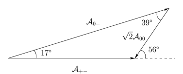
FIG. 1.:

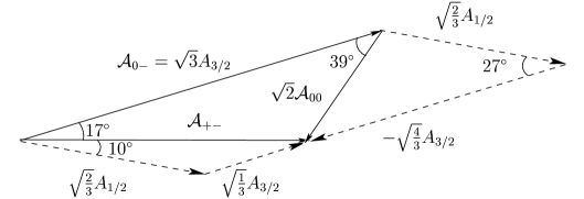
FIG. 2.:

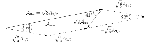
FIG. 3.:

TABLE I.:

	NRSX	LF	MS	NS
$F_{0}^{B\pi}(m_{D}^{2})$	0.37	0.34	0.32	0.27
$F_{0}^{BD}(m_{\pi}^{2})$	0.69	0.70	0.67	0.63
$a_{2}(D\pi)$	0.39$e^{i56^{\circ}}$	0.43$e^{i56^{\circ}}$	0.45$e^{i56^{\circ}}$	0.54$e^{i56^{\circ}}$
$\tilde{a}_{2}(D^{*}\pi)$	0.26$e^{i52^{\circ}}$	0.30$e^{i52^{\circ}}$	0.32$e^{i52^{\circ}}$	0.36$e^{i52^{\circ}}$
$|\epsilon_{\rm NF}^{B\pi,D}/f_{D}|$	0.31	0.34	0.36	0.44
$|\epsilon_{\rm NF}^{B\pi,D^{*}}/f_{D^{*}}|$	0.19	0.22	0.24	0.28
$R_{\rm NF}$	0.72	0.76	0.77	0.73

REFERENCES

• [1] M.Β Beneke, G.Β Buchalla, M.Β Neubert, C.T.Β Sachrajda, Phys. Rev. Lett. 83, 1914 (1999); Nucl. Phys. B591, 313 (2000).
• [2] M.Β Neubert, [hep-ph/0012204].
• [3] J.Β Chay, [hep-ph/0101169].
• [4] K.Β Abe et al., Belle Collaboration, [hep-ex/0107048].
• [5] D.Β Cassel, talk given at the 20th International Symposium on Lepton and Photon Interactions at High Energies (Lepton Photon 01), July 2001, Rome, Italy.
• [6] Z.Β Xing, [hep-ph/0107257].
• [7] H.-Y.Β Cheng, [hep-ph/010896].
• [8] M.Β Neubert and A.A.Β Petrov, [hep-ph/0108103].
• [9] M.Β Neubert, V.Β Rieckert, B.Β Stech, Q.P.Β Xu, in Heavy Flavours, 1st edition, ed. A.J.Β Buras and M.Β Linder (World Scientific, Singapore, 1992).
• [10] H.-Y.Β Cheng, C.Y.Β Cheung, C.W. Hwang, Phys. Rev. D 55, 1559 (1997).
• [11] M.Β Neubert and B.Β Stech, in: Heavy Flavours II, ed. A.J.Β Buras and M.Β Lindner (World Scientific, Singapore, 1998), pp. 294 [hep-ph/9705292].
• [12] D.Β Melikhov and B.Β Stech, Phys. Rev. D 62, 014006 (2001).
• [13] Particle Data Group, D.E.Β Groom et al., Eur. Phys. J. C 15, 1 (2000).
• [14] A.Β Deandrea, N.Β Di Bartolomeo, R.Β Gatto, G.Β Nardulli, Phys. Lett. B 318, 549 (1993).
• [15] H.-Y.Β Cheng and K.-C.Β Yang, Phys. Rev. D 59, 092004 (1999).
• [16] N.Β Isgur, M.B.Β Wise, Phys. Lett. B 232, 113 (1989); ibid. B 237, 527 (1990); H.Β Georgi, ibid. B 240, 447 (1990).
FIGURE CAPTIONS