Abstract

We estimate the decay width difference $\Delta\Gamma_{d}/\Gamma_{d}$ in the $B_{d}$ system including $1/m_{b}$ contributions and part of the next-to-leading order QCD corrections, and find it to be around $0.3\%$. We explicitly show that the time measurements of an untagged $B_{d}$ decaying to a single final state isotropically can only be sensitive to quadratic terms in $\Delta\Gamma_{d}/\Gamma_{d}$, and hence the use of at least two different final states is desired. We discuss such pairs of candidate decay channels for the final states and explore the feasibility of a $\Delta\Gamma_{d}/\Gamma_{d}$ measurement through them. The measurement of $\Delta\Gamma_{d}$ would be essential for an accurate measurement of $\sin(2\beta)$ at the LHC. The nonzero width difference can also be used to identify new physics effects and to resolve a twofold discrete ambiguity in the $B_{d}$–$\bar{B}_{d}$ mixing phase. We also derive an upper bound on the value of $\Delta\Gamma_{d}/\Gamma_{d}$ in the presence of new physics, and point out some differences in the phenomenology of width differences in the $B_{s}$ and $B_{d}$ systems.

1 Introduction

Within the standard model (SM), the difference in the decay widths of $B_{d}$ mesons is CKM-suppressed with respect to that in the $B_{s}$ system. A rough estimate leads to

$$\frac{\Delta\Gamma_{d}}{\Gamma_{d}}\sim\frac{\Delta\Gamma_{s}}{\Gamma_{s}}\cdot\lambda^{2}\approx 0.5\%~{}~{},$$ (1)

where $\lambda=0.225$ is the sine of Cabibbo angle, and we have taken $\Delta\Gamma_{s}/\Gamma_{s}\approx 15\%$ [1, 2, 3]. Here $\Gamma_{d(s)}=(\Gamma_{L}+\Gamma_{H})/2$ is the average decay width of the light and heavy $B_{d(s)}$ mesons ($B_{L}$ and $B_{H}$ respectively). We denote these decay widths by $\Gamma_{L},\Gamma_{H}$ respectively, and define $\Delta\Gamma_{d(s)}\equiv\Gamma_{L}-\Gamma_{H}$. No experimental measurement of $\Delta\Gamma_{d}$ is currently available. Moreover, no motivation for its measurement (other than just measuring another number to check against the SM prediction) has been discussed, and hence the study of the lifetime difference between $B_{d}$ mesons has hitherto been neglected as compared to that in the $B_{s}$ system. The phenomenology of the lifetime difference between $B_{s}$ mesons has been explored in detail in [4, 5].

With the possibility of experiments with high time resolution and high statistics, it is worthwhile to have a look at this quantity and make a realistic estimate of the possibility of its measurement. At LHCb for example, the proper time resolution is expected to be as good as $\Delta\tau\approx 0.03$ ps. This indeed is a very small fraction of the $B_{d}$ lifetime ($\tau_{B_{d}}\approx 1.5$ ps [6]), so the time resolution is not a limiting factor in the accuracy of the measurement, the statistical error plays the dominant role. Taking into account the estimated number of $B_{d}$ produced — for example the number of reconstructed $B_{d}\rightarrow J/\psi\,K_{S}$ events at the LHC is expected to be $5\times 10^{5}$   ([7] table 3) — the measurement of the lifetime difference does not look too hard at first glance. Naively, one may infer that if the number of relevant events with the proper time of decay measured with the precision $\Delta\tau$ is $N$, then the value of $\Delta\Gamma_{d}/\Gamma_{d}$ is measured with an accuracy of $1/\sqrt{N}$. With a sufficiently large number of events $N$, it should be possible to reach the accuracy of 0.5% or better.

The measurement of $\Delta\Gamma_{d}/\Gamma_{d}$ is in reality harder than what the above naive expectation may suggest, since most of the quantities that involve the lifetime difference are quadratic in the small quantity $\Delta\Gamma_{d}/\Gamma_{d}$. In fact, as we shall explicitly show in this paper, the time measurements in the decays of an untagged $B_{d}$ to a single final state are sensitive only to $(\Delta\Gamma_{d}/\Gamma_{d})^{2}$. This implies that in order to discern two different lifetimes, the measurements need to have an accuracy of $(\Delta\Gamma_{d}/\Gamma_{d})^{2}\sim 2.5\times 10^{-5}$, which is beyond the reach of the currently planned experiments.

However, the combination of lifetimes measured in two different untagged decay channels may be sensitive to linear terms in $\Delta\Gamma_{d}/\Gamma_{d}$. We explore three pairs of such untagged measurements in this paper: (i) lifetime measurements through decays to self-tagging (e.g. semileptonic) final states and to CP eigenstates, (ii) CP even and odd components in the decay mode $B_{d}\to J/\psi K^{*}(K_{s}\pi^{0})$, and (iii) time-dependent untagged asymmetry between $B_{d}\to J/\psi K_{S}$ and $B_{d}\to J/\psi K_{L}$.

The conventional “gold-plated” decays for $\beta$ measurement, $J/\psi K_{S}$ and $J/\psi K_{L}$, neglect the lifetime difference while determining $\sin(2\beta)$. For an accurate determination of $\beta$, the systematic errors due to $\Delta\Gamma_{d}/\Gamma_{d}$ need to be taken into account. Moreover, there is the possibility that the measurement of the lifetime difference leads to a clear signal for new physics. Furthermore, if the lifetime difference is neglected, the ambiguity $\beta\leftrightarrow(\pi/2-\beta)$ remains unresolved. Observables that are sensitive to the lifetime difference may resolve this discrete ambiguity under certain conditions.

The observables mentioned above can also give an independent measurement of $\cos(2\beta)$ in principle. In order to be able to do this, however, the theoretical uncertainties on $\Delta\Gamma_{d}$ need to be minimized. Therefore, we start by presenting in Sec. 2 a detailed calculation of $\Delta\Gamma_{d}$, including $1/m_{b}$ contributions and part of the next-to-leading order (NLO) QCD corrections. The NLO precision in the width difference $\Delta\Gamma_{d}$ is also essential for obtaining a proper matching of the Wilson coefficients to the matrix elements of local operators from the lattice gauge theory.

The rest of the paper is organized as follows. In Sec. 3 we explicitly demonstrate the quadratic dependence on $\Delta\Gamma_{d}/\Gamma_{d}$ of quantities measurable through untagged $B$ decays to a single final state. We explore the combinations of decay modes that can measure quantities linear in $\Delta\Gamma_{d}/\Gamma_{d}$. We calculate the corrections due to $\Delta\Gamma_{d}$ to the measurement of $\sin(2\beta)$ through $B_{d}\to J/\psi K_{S}$, and also indicate the possibility of the $\Delta\Gamma_{d}$ measurement through tagged decays to CP eigenstates. In Sec. 4, we point out important differences in the upper bounds on $\Delta\Gamma_{s}$ and $\Delta\Gamma_{d}$ in the presence of new physics, and elaborate on the possibility of detecting new physics and resolving discrete ambiguities in the mixing phases through them. We summarize our findings in Sec. 5.

2 Estimation of $\Delta\Gamma_{d}$

2.1 Basic definitions

We briefly recall the basic definitions: in the Wigner–Weisskopf approximation the oscillation and the decay of a general linear combination of the neutral flavour eigenstates $B_{d}$ and $\bar{B}_{d}$,  $a|{B_{d}}\rangle+b|{\bar{B}_{d}}\rangle$,  is described by the time-dependent Schrödinger equation

$$i{d\over dt}\pmatrix{a\cr b\cr}=\left({\bf M}-{i\over 2}{\bf\Gamma}\right)\pmatrix{a\cr b\cr}.$$ (2)

Here ${\bf M}$ and ${\bf\Gamma}$ are $2\times 2$ Hermitean matrices. CPT invariance leads to the conditions ${M_{11}}={M_{22}}$ and ${\Gamma_{11}}={\Gamma_{22}}$. Exact CP invariance would imply ${M_{21}}={M_{12}}$ and ${\Gamma_{21}}={\Gamma_{12}}$ (a phase choice, namely ${\cal CP}|{B_{d}}\rangle=-|{\bar{B}_{d}}\rangle$$,{\cal CP}|{\bar{B}_{d}}\rangle=-|{B_{d}}\rangle$ is made). Independent of the choice of the unphysical phases, CP invariance (in mixing) would imply ${\rm Im}({M^{*}_{21}\Gamma_{21}})=0$.

The mass eigenstates, the light $B_{L}$ and the heavy $B_{H}$, are given by

$$|{B_{L,H}}\rangle=p|{B_{d}}\rangle\pm q|{\bar{B}_{d}}\rangle$$ (3)

with the normalization condition $|q|^{2}+|p|^{2}=1$. Only the magnitude $|q/p|$ is measurable, the phase of this quantity is unphysical and can be fixed arbitrarily by convention.

The mass difference and the width difference between the physical states are defined by

$$\Delta m=M_{H}-M_{L},\quad\Delta\Gamma=\Gamma_{L}-\Gamma_{H}~{},$$ (4)

such that $\Delta m>0,\Delta\Gamma_{d}>0$ in the SM. The real and imaginary parts of the eigenvalue equations are the following:

$$(\Delta m)^{2}-{1\over 4}(\Delta\Gamma)^{2}\ = \ (4|M_{21}|^{2}-|\Gamma_{21}|^{2}),$$ (5)

$$\Delta m\Delta\Gamma\ = \ -4{\rm Re}(M_{21}^{*}\Gamma_{21}).$$ (6)

With the help of the CP-violating parameter $\delta$

$$\delta\equiv\frac{-2~{}{\rm Im}({M^{*}_{21}\Gamma_{21}})}{(\Delta m)^{2}+|\Gamma_{21}|^{2}}=|p|^{2}-|q|^{2}=\langle B_{L}|B_{H}\rangle,$$ (7)

The effect of CP violation due to mixing on the mass difference $\Delta m$ and on the lifetime difference $\Delta\Gamma$ may be explicitly shown:

$$(\Delta m)^{2} = \frac{4|M_{21}|^{2}-\delta^{2}|\Gamma_{21}|^{2}}{1+\delta^{2}}$$ (8)

$$(\Delta\Gamma)^{2} = \frac{4|\Gamma_{21}|^{2}-16\delta^{2}|M_{21}|^{2}}{1+\delta^{2}}~{}.$$ (9)

In the limit of exact CP invariance ($\delta=0$) the mass eigenstates coincide with the CP eigenstates,   ${\cal CP}|B_{H}\rangle=-|B_{H}\rangle$ and ${\cal CP}|B_{L}\rangle=+|B_{L}\rangle$ and the mass difference and width difference are given by $\Delta m=2|M_{21}|,\Delta\Gamma=2|\Gamma_{21}|$. However, even with a non-zero $\delta$, taking into account that $\delta$ is constrained by the upper bound $|\delta|\leq|\Gamma_{21}|/(2|M_{21}|)$ and $\Gamma_{21}/M_{21}={\cal O}(m_{b}^{2}/m_{t}^{2})$, we can write

$$\Delta m=2|M_{21}|\left[1+{\cal O}\left(\frac{m_{b}^{4}}{m_{t}^{4}}\right)\right],\quad\Delta\Gamma=-\frac{2{\rm Re}(M_{21}^{*}\Gamma_{21})}{|M_{21}|}\left[1+{\cal O}\left(\frac{m_{b}^{4}}{m_{t}^{4}}\right)\right].$$ (10)

We shall neglect the terms of ${\cal O}(m_{b}^{4}/m_{t}^{4})\sim 10^{-6}$ in our calculations.

2.2 Method of calculation

In the following we consider the two off-diagonal elements $M_{21}$ and $\Gamma_{21}$, which correspond respectively to the dispersive and the absorptive part of the transition amplitude from $B_{d}$ to $\bar{B}_{d}$. We follow the method of [2, 3] which was used there in the $B_{s}$–$\bar{B}_{s}$ system (see also [8, 9]).

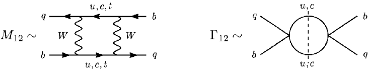
Figure 1: Schematic representation of Feynman diagrams for $M_{12}=M_{21}^{*}$ and $\Gamma_{12}=\Gamma_{21}^{*}$.

Within the SM the well-known box diagram is the starting point of the calculations. $M_{21}$ is related to the real part of this diagram (see Fig. 1). The important QCD corrections are most easily implemented with the help of the standard operator product expansion. Because of the dominance of the top quark contribution, $M_{21}$ can be described by a local $\Delta B=2$ Hamiltonian below the $m_{W}$ scale:

$$M_{21} = \frac{1}{2M_{B_{d}}}\langle\bar{B}_{d}|{\cal H}_{eff}^{\Delta B=2}|B_{d}\rangle\,\left[1+O\left(\frac{m_{b}^{2}}{m_{W}^{2}}\right)\right]~{}~{},$$ (11)

$${\cal H}_{eff}^{\Delta B=2} = \frac{G_{F}^{2}}{16\pi^{2}}(V_{tb}^{*}V_{td})^{2}C^{Q}(m_{t},m_{W},\mu)Q(\mu)+{\rm H.c.}~{}~{},$$ (12)

$$Q = (\overline{b}_{i}d_{i})_{V-A}(\bar{b}_{j}d_{j})_{V-A}~{}~{}.$$ (13)

The Wilson coefficient $C^{Q}$ contains the short-distance physics. It is known up to NLO precision [10]. The hadronic matrix element $\langle\bar{B}_{d}|Q(\mu\approx m_{b})|B_{d}\rangle$ will be discussed below.

In the standard model, $\Gamma_{21}$ is related to the imaginary part of the box diagram. Via the optical theorem it is fixed by the real intermediate states. Therefore, only the box diagrams with internal $c$ and $u$ quarks contribute (see Fig. 1). In contrast to the $B_{s}$–$\bar{B}_{s}$ case where the intermediate $c\bar{c}$ contribution is the dominating one, because of its CKM factor $(V_{cb}^{*}V_{cs})^{2}$, over the $u\bar{u}$, the $c\bar{u}$ and the $u\bar{c}$ contribution (see Sec. 4.1), in the $B_{d}$–$\bar{B}_{d}$ all four contributions have to be taken into account. In the effective theory where we integrate out the $W$ boson, $\Gamma_{21}$ is given by:

$$\Gamma_{21}=\frac{1}{2M_{B_{d}}}\langle\bar{B}_{d}|{\rm Im}~{}i\int d^{4}x~{}T~{}{\cal H}^{\Delta B=1}_{eff}(x)\,~{}{\cal H}^{\Delta B=1}_{eff}(0)|B_{d}\rangle~{}~{},$$ (14)

where

$${\cal H}^{\Delta B=1}_{eff} = \frac{G_{F}}{\sqrt{2}}(V_{ub}^{*}V_{ud}\sum_{i=1,2}C_{i}Q_{i}^{uu}+V_{cb}^{*}V_{ud}\sum_{i=1,2}C_{i}Q_{i}^{cu}+V_{ub}^{*}V_{cd}\sum_{i=1,2}C_{i}Q_{i}^{uc}+$$ (15)

$$+ V_{cb}^{*}V_{cd}\sum_{i=1,2}C_{i}Q_{i}^{cc}-V_{tb}^{*}V_{td}\sum_{i=3}^{6}C_{i}Q_{i}).$$

The operators are ($i,j$ denote color indices)

$$Q_{1}^{qq^{\prime}} = (\overline{b}_{i}q_{j})_{V-A}(\bar{q}^{\prime}_{j}d_{i})_{V-A},\,\,\,\,\,\,Q_{2}^{qq^{\prime}}=(\overline{b}_{i}q_{i})_{V-A}(\bar{q}^{\prime}_{j}d_{j})_{V-A},$$ (16)

$$Q_{3} = (\overline{b}_{i}d_{i})_{V-A}(\bar{q}_{j}q_{j})_{V-A},\,\,\,\,\,\,\,\,\,\,Q_{4}=(\overline{b}_{i}d_{j})_{V-A}(\bar{q}_{j}q_{i})_{V-A},$$ (17)

$$Q_{5} = (\overline{b}_{i}d_{i})_{V-A}(\bar{q}_{j}q_{j})_{V+A},\,\,\,\,\,\,\,\,\,\,Q_{6}=(\overline{b}_{i}d_{j})_{V-A}(\bar{q}_{j}q_{i})_{V+A}.$$ (18)

The penguin operators $Q_{3}$ – $Q_{6}$ have small Wilson coefficients and are therefore suppressed with respect to the four-quark operators – which all have the same two Wilson coefficients $C_{1}$ and $C_{2}$. In the leading logarithmic approximation we have:

$$C_{\pm}=C_{2}\pm C_{1},\quad C_{\pm}(\mu)=\left(\frac{\alpha(M_{W})}{\alpha(\mu)}\right)^{\frac{\gamma^{(0)}_{\pm}}{2\beta_{0}}}C_{\pm}(M_{W}),\quad C_{\pm}(M_{W})=1~{}~{},$$ (19)

where $\beta_{0}=(11N-2f)/{3}=23/3$ and $\gamma^{(0)}_{\pm}=\pm 6(1\pm N)/N$. The coefficients to NLO precision can be found in [11].

Because there is another short-distance scale, the bottom quark mass, the operator product of two $\Delta B=1$ operators can be expanded in inverse powers of the bottom quark mass scale in terms of local $\Delta B=2$ operators:

$$\Gamma_{21} = \frac{1}{2M_{B_{d}}}\langle\bar{B}_{d}|{\rm Im}\,i\int d^{4}xT{\cal H}^{\Delta B=1}_{eff}(x){\cal H}^{\Delta B=1}_{eff}(0)|B_{d}\rangle$$ (20)

$$= \sum_{n}\frac{E_{n}}{m_{b}^{n}}\,\langle\bar{B}_{d}|{\cal O}_{n}^{\Delta B=2}(0)|B_{d}\rangle~{}~{}.$$ (21)

These matching equations fix the values of the $\Delta B=2$ Wilson coefficients $E_{n}$. The corresponding four quark operators ${\cal O}_{n}$ are the following: The operators $Q$ and $Q_{S}$,

$$Q = (\overline{b}_{i}d_{i})_{V-A}(\overline{b}_{j}d_{j})_{V-A},$$ (22)

$$Q_{S} = (\overline{b}_{i}d_{i})_{S-P}(\overline{b}_{j}d_{j})_{S-P},$$ (23)

represent the leading order contributions. Their matrix elements are given in terms of the bag parameters, $B$ and $B_{S}$, the mass of the $B_{d}$ meson $M_{B_{d}}$, and its decay constant $f_{B_{d}}$:

$$\langle\bar{B}_{d}|Q|B_{d}\rangle = f_{B_{d}}^{2}M_{B_{d}}^{2}2\frac{N+1}{N}B,$$ (24)

$$\langle\bar{B}_{d}|Q_{S}|B_{d}\rangle = -f_{B_{d}}^{2}M_{B_{d}}^{2}\frac{M_{B_{d}}^{2}}{(\bar{m}_{b}+\bar{m_{d}})^{2}}\frac{2N-1}{N}B_{S}~{}~{}.$$ (25)

In the naive factorization approximation, $B$ and $B_{S}$ are fixed by $B=B_{S}=1$. Reliable lattice calculations for $B$ and $B_{S}$ are already available [12]. We note that to NLO precision one has to distinguish between the pole mass $m_{b}$ and the running quantity

$$\bar{m}_{b}(\mu)=m_{b}\left[1-\frac{\alpha_{s}}{\pi}\,\,\left(ln\frac{\mu^{2}}{m_{b}^{2}}+\frac{4}{3}\right)\right]$$ (26)

using the $\overline{MS}$ scheme.

The $1/m_{b}$ corrections are given by the operators

$$R_{1} = \frac{m_{d}}{m_{b}}(\bar{b}_{i}d_{i})_{S-P}(\bar{b}_{j}d_{j})_{S+P},$$ (27)

$$R_{2} = \frac{1}{m^{2}_{b}}(\bar{b}_{i}{\overleftarrow{D}}_{\!\rho}\gamma^{\mu}(1-\gamma_{5})D^{\rho}d_{i})(\bar{b}_{j}\gamma_{\mu}(1-\gamma_{5})d_{j}),$$ (28)

$$R_{3} = \frac{1}{m^{2}_{b}}(\bar{b}_{i}{\overleftarrow{D}}_{\!\rho}(1-\gamma_{5})D^{\rho}d_{i})(\bar{b}_{j}(1-\gamma_{5})d_{j}),$$ (29)

$$R_{4} = \frac{1}{m_{b}}(\bar{b}_{i}(1-\gamma_{5})iD_{\mu}d_{i})(\bar{b}_{j}\gamma^{\mu}(1-\gamma_{5})d_{j}),$$ (30)

$$R_{0} = Q_{S}+\frac{1}{2}\,Q+\tilde{Q}_{S},$$ (31)

where $\tilde{Q}_{S}$ has the “interchanged” color structure as compared to $Q_{S}$. There are also “color-interchanged” operators $\tilde{R}_{i}$ and $\tilde{Q}$ corresponding to $R_{i}$ and $Q$. We note that these $1/m_{b}$ operators are not independent, the relations between them are in fact the equations of motion.

The matrix elements of these operators within the $B_{s}$–$\bar{B}_{s}$ system were estimated in [2] using naive factorization, which means that all the corresponding bag factors were set to $1$. For the $B_{d}$–$\bar{B}_{d}$ system the analogous results are:

$$\langle\bar{B}_{d}|R_{0}|B_{d}\rangle = f^{2}_{B_{d}}M^{2}_{B_{d}}\left(\frac{N+1}{N}\right)\left(1-\frac{M^{2}_{B_{d}}}{m_{b}^{2}}\right)~{},$$ (32)

$$\langle\bar{B}_{d}|R_{1}|B_{d}\rangle = f_{B_{d}}^{2}M_{B_{d}}^{2}\frac{m_{d}}{m_{b}}\frac{2N+1}{N}=0~{},$$ (33)

$$\langle\bar{B}_{d}|\tilde{R}_{1}|B_{d}\rangle = f_{B_{d}}^{2}M_{B_{d}}^{2}\frac{m_{d}}{m_{b}}\frac{N+2}{N}=0~{},$$ (34)

$$\langle\bar{B}_{d}|R_{2}|B_{d}\rangle = f_{B_{d}}^{2}M_{B_{d}}^{2}\left(\frac{M_{B_{d}}^{2}}{m_{b}^{2}}-1\right)\frac{1-N}{N}\,=\,-\langle\bar{B}_{d}|\tilde{R}_{2}|B_{d}\rangle~{},$$ (35)

$$\langle\bar{B}_{d}|R_{3}|B_{d}\rangle = f_{B_{d}}^{2}M_{B_{d}}^{2}\left(\frac{M_{B_{d}}^{2}}{m_{b}^{2}}-1\right)\frac{2N+1}{2N}~{},$$ (36)

$$\langle\bar{B}_{d}|\tilde{R}_{3}|B_{d}\rangle = f_{B_{d}}^{2}M_{B_{d}}^{2}\left(\frac{M_{B_{d}}^{2}}{m_{b}^{2}}-1\right)\frac{N+2}{2N}~{},$$ (37)

$$\langle\bar{B}_{d}|R_{4}|B_{d}\rangle = -f_{B_{d}}^{2}M_{B_{d}}^{2}\left(\frac{M_{B_{d}}^{2}}{m_{b}^{2}}-1\right)~{},$$ (38)

$$\langle\bar{B}_{d}|\tilde{R}_{4}|B_{d}\rangle = -f_{B_{d}}^{2}M_{B_{d}}^{2}\left(\frac{M_{B_{d}}^{2}}{m_{b}^{2}}-1\right)\frac{1}{N}~{}~{}.$$ (39)

We neglect terms proportional to $m_{d}/m_{b}$; the other terms proportional to $(M_{B_{d}}^{2}/m_{b}^{2})-1$ are of order $\Lambda_{QCD}/m_{b}$.

In the matrix elements $\langle R_{i}\rangle$ (eqs. (32)–(39)), we use the pole mass $m_{b}$. There is a subtlety involved here: as discussed in [3], there are terms of order $\alpha_{s}$ and of leading power in $m_{b}$ in the matrix element of $R_{0}$ to NLO precision. In view of the relation (31), it is not surprising that there are such terms. In the scheme – which was used in [3] and which is also used here – these terms are subtracted in the matrix element $\langle R_{0}\rangle$ while taking into account the leading NLO contribution. Then the $\langle R_{0}\rangle$ matrix element is still of a subleading nature. The specific subtraction scheme for the factorized matrix elements $\langle R_{i}\rangle$ corresponds to the use of the pole mass in eqs. (32)–(39). Of course this specific choice for the matrix elements has to be taken into account if the NLO results are combined with a lattice calculation of the $\langle R_{i}\rangle$.

There is an additional remark in order. We estimate $\Gamma_{21}$ by the cut of the partonic diagrams. The underlying assumption of local quark-hadron duality can be verified in the $B_{s}$–$\bar{B}_{s}$ system, in the simultaneous limit of large $N$ and of small velocity [1], therefore one expects no large duality violations. In the $B_{d}$–$\bar{B}_{d}$ system the small velocity argument fails since the $u\bar{u}$, $u\bar{c}$ and $c\bar{u}$ intermediate states contribute significantly, and the larger number of light intermediate states leads to a larger energy release. We follow ref. [2] and make the assumption that the duality violations in the $B_{d}-\bar{B}_{d}$ system are also not larger than $10\%$. In order to test this assumption one should include all corrections up to that accuracy.

2.3 Analytical results

In this section, we present an analytic expression for $\Gamma_{21}$ including $1/m_{b}$, penguin and part of the NLO corrections. If one takes into account the error inherent in the naive factorization approach to the matrix elements of the subleading operators $R$, it seems to be a reasonable approximation to keep at least all terms up to an accuracy of $10^{-2}~{}\Gamma_{21}^{leading}$. We keep also higher order terms in order to check the accuracy of our approximation.

In the effective theory of the $\Delta B=2$ transitions the matrix elements of the $1/m_{b}$ operators ($R$) are formally suppressed by a factor of the order of $0.1$ with respect to those of the leading operators $Q$ and $Q_{S}$. The natural variable $z=m_{c}^{2}/m_{b}^{2}$ also formally introduces a suppression factor of approximately $0.1$. The NLO contribution has formally an extra suppression factor $(\alpha_{s}/4\pi)$ of order $0.01$. Within the effective theory of the $\Delta B=1$ Hamiltonian, the combination $K^{\prime}=C^{peng}C^{dom}$ and $K^{\prime\prime}=C^{peng}C^{peng}$ are suppressed by almost a factor 0.01 and $10^{-4}$ respectively, with respect to the combination $K=C^{dom}C^{dom}$, where $C^{peng}$ denotes the Wilson coefficients of the penguin operators $Q_{3}...Q_{6}$ and $C^{dom}$ that of the dominating operators $Q^{qq^{\prime}}_{1\,(2)}$. The contribution due to $K^{\prime\prime}$ therefore can be safely neglected. Schematically our analytical result for $\Gamma_{21}$ has the following form:

$$\Gamma_{21} = \,K\,\langle{\cal Q}\rangle$$ (40)

$$+ \,K\,\langle R\rangle\,(O(1)+O(z)+O(z^{2})+\{O(z^{3})\})$$ (41)

$$+ \,K^{\prime}\,\langle{\cal Q}\rangle\,(O(1)+O(z)+\{O(z^{2})\})$$ (42)

$$+ \,K^{\prime}\,\langle R\rangle\,(O(1)+\{O(z^{2})\}$$ (43)

$$+ \,\alpha_{s}/(4\pi)\,\,K\,\langle{\cal Q}\rangle\,O(1)~{}~{},$$ (44)

where ${\cal Q}$ represents the leading order operators $Q$ and $Q_{S}$. The terms inside the curly brackets are the ones that we calculate only to estimate the errors. In the presentation of the results the following combinations of the Wilson coefficients are used:

$$K_{1} = 3C_{1}^{2}+2C_{1}C_{2},\quad K_{2}=C_{2}^{2},\quad K_{3}=C_{1}^{2},\quad K_{4}=C_{1}C_{2}$$ (45)

$$K_{1}^{\prime} = 2(3C_{1}C_{3}+C_{1}C_{4}+C_{2}C_{3}),~{}~{}K_{2}^{\prime}=2C_{2}C_{4},$$ (46)

$$K_{3}^{\prime} = 2(3C_{1}C_{5}+C_{1}C_{6}+C_{2}C_{5}+C_{2}C_{6}),$$ (47)

and the common factor of $[-G_{F}^{2}m_{b}^{2}/(24\pi M_{B_{d}})]$ is implicit in the following equations (48), (49), (51), (53).

In the leading log approximation we calculate the $Q^{qq^{\prime}}_{1}$ and the $Q^{qq^{\prime}}_{2}$ contributions to $\Gamma_{21}$. By extracting the absorptive parts of the $c\bar{c},u\bar{c},c\bar{u}$ and $u\bar{u}$ intermediate states, we can find the off-diagonal element. For this leading contribution (40), after replacing $V_{ub}^{*}V_{ud}$ by the unitarity relation, we get to all orders in $z$:

$$\Gamma^{leading}_{21} = (V_{tb}^{*}V_{td})^{2}\left[\left(K_{1}+\frac{1}{2}K_{2}\right)\langle Q\rangle+(K_{1}-K_{2})\langle Q_{S}\rangle\right]$$ (48)

$$+ (V_{cb}^{*}V_{cd})(V_{tb}^{*}V_{td})\Bigl{[}(3z(K_{1}+K_{2})-3z^{2}K_{2}-z^{3}(K_{1}-K_{2}))\langle Q\rangle$$

$$\quad\quad\quad\quad+(6z^{2}(K_{1}-K_{2})-4z^{3}(K_{1}-K_{2}))\langle Q_{S}\rangle\Bigr{]}$$

$$+ (V_{cb}^{*}V_{cd})^{2}\Bigl{\{}\sqrt{1-4z}\left[\left(K_{1}+\frac{1}{2}K_{2}\right)-z(K_{1}+2K_{2})\right]\langle Q\rangle$$

$$\quad\quad\quad\quad+\sqrt{1-4z}(1+2z)(K_{1}-K_{2})\langle Q_{s}\rangle$$

$$\quad\quad\quad\quad+\left((1-z)^{2}\left[-(2K_{1}+K_{2})+z(K_{2}-K_{1})\right]+\left[K_{1}+\frac{1}{2}K_{2}\right]\right)\langle Q\rangle$$

$$\quad\quad\quad\quad+\left[(1-z)^{2}(2+4z)(K_{2}-K_{1})-(K_{2}-K_{1})\right]\langle Q_{S}\rangle\Bigr{\}}~{}~{}.$$

This result, (48), confirms the findings of [9].

In the equations (49),(50), (51), and (52) we give the penguin and $1/m_{b}$ contributions. The coefficients of $(V_{tb}^{*}V_{td})^{2}$ in these results can be checked with the $z\to 0$ limit of the results in the literature for the $B_{s}$ syatem. In this sense our results are consistent with the findings in the $B_{s}$ system given in [2].

The $1/m_{b}$ corrections to the operators $Q^{qq^{\prime}}_{1}$ and $Q^{qq^{\prime}}_{2}$ give [see the term (41)]

$$\Gamma^{1/m_{b}}_{21} = (V_{tb}^{*}V_{td})^{2}\left[-2\left(K_{1}-\frac{1}{2}K_{2}\right)\langle R_{2}\rangle-2K_{1}\langle R_{1}\rangle+2K_{2}\langle R_{4}\rangle\right]$$ (49)

$$+ (V_{cb}^{*}V_{cd})(V_{tb}^{*}V_{td})\Bigl{[}-12z^{2}K_{1}(\langle R_{1}\rangle-2\langle R_{3}\rangle)$$

$$~{}~{}~{}~{}~{}~{}~{}~{}~{}~{}~{}~{}~{}~{}~{}~{}~{}~{}~{}~{}+6z^{2}K_{2}(\langle R_{2}\rangle+4\langle R_{3}\rangle+2\langle R_{4}\rangle)\Bigr{]}$$

$$+ \Bigl{\{}K\langle R\rangle O(z^{3})\Bigr{\}}.$$

The term in curly brackets in (49) can be written as

$$\{...\} = (V_{cb}^{*}V_{cd})(V_{tb}^{*}V_{td})\times$$ (50)

$$[4z^{3}K_{1}(2\langle R_{1}\rangle-\langle R_{2}\rangle-6\langle R_{3}\rangle)-4z^{3}K_{2}(\langle R_{2}\rangle+6\langle R_{3}\rangle+2\langle R_{4}\rangle)]$$

$$+ (V_{cb}^{*}V_{cd})^{2}\times$$

$$[12z^{3}K_{1}(2\langle R_{1}\rangle-\langle R_{2}\rangle-6\langle R_{3}\rangle)-12z^{3}K_{2}(\langle R_{2}\rangle+6\langle R_{3}\rangle+2\langle R_{4}\rangle)]~{}~{}.$$

The penguin contributions [terms (42), (43)] are

$$\Gamma^{peng}_{21} = (V_{tb}^{*}V_{td})^{2}\Bigl{[}\left(K_{1}^{\prime}+\frac{1}{2}K_{2}^{\prime}\right)\langle Q\rangle+(K_{1}^{\prime}-K_{2}^{\prime})\langle Q_{S}\rangle$$ (51)

$$~{}~{}~{}~{}~{}~{}~{}~{}~{}+(-2\langle R_{2}\rangle-2\langle R_{1}\rangle)K_{1}^{\prime}+(\langle R_{2}\rangle+2\langle R_{4}\rangle)K_{2}^{\prime}\Bigr{]}$$

$$+ (V_{cb}^{*}V_{cd})(V_{tb}^{*}V_{td})(3zK_{1}^{\prime}+3zK_{2}^{\prime}-3zK_{3}^{\prime})\langle Q\rangle$$

$$+\bigl{\{}K^{\prime}\,\langle{\cal Q}\rangle\,O(z^{2})+\,K^{\prime}\,\langle R\rangle\,O(z)\bigr{\}}~{}~{},$$

where the terms in curly brackets (and the lower order ones) may be written as

$$\{...\} = (V_{cb}^{*}V_{cd})(V_{tb}^{*}V_{td})\times$$ (52)

$$\Bigl{[}~{}~{}(-3z^{2}K_{2}^{\prime}+6z^{2}K_{3}^{\prime})\langle Q\rangle+(6z^{2}K_{1}^{\prime}-6z^{2}K_{2}^{\prime})\langle Q_{S}\rangle$$

$$-(12z^{2}\langle R_{1}\rangle-24z^{2}\langle R_{3}\rangle)K_{1}^{\prime}$$

$$+(6z^{2}\langle R_{2}\rangle+24z^{2}\langle R_{3}\rangle+12z^{2}\langle R_{4}\rangle)K_{2}^{\prime}+4z^{2}\langle R_{2}\rangle K_{3}^{\prime}~{}~{}\Bigr{]}~{}.$$

The NLO QCD correction $\Gamma^{NLO}_{21}=\alpha_{s}/(4\pi)\,\,K\,\langle{\cal Q}\rangle$ [term (44)] is found from [3] by taking the limit $z\rightarrow 0$ of their results:

$$\Gamma^{NLO}_{21} = \frac{\alpha_{s}(m_{b})}{4\pi}(V_{tb}^{*}V_{td})^{2}\Bigl{\{}\left[\frac{109}{6}K_{3}-\frac{248}{9}K_{4}-\left(\frac{\pi^{2}}{3}+\frac{157}{18}\right)K_{2}\right]\langle Q\rangle$$ (53)

$$\quad\quad+\left[\left(10K_{3}+\frac{20}{3}K_{4}+\frac{8}{3}K_{2}\right){\rm ln}\left(\frac{\mu_{2}}{m_{b}}\right)-(34K_{4}+10K_{2}){\rm ln}\left(\frac{\mu_{1}}{m_{b}}\right)\right]\langle Q\rangle$$

$$\quad\quad-\left[\frac{40}{3}K_{3}+\frac{248}{9}K_{4}-\left(\frac{8\pi^{2}}{3}-\frac{128}{9}\right)K_{2}\right]\langle Q_{S}\rangle$$

$$\quad\quad+\left[\left(32K_{3}-\frac{64}{3}K_{4}+\frac{32}{3}K_{2}\right){\rm ln}\left(\frac{\mu_{2}}{m_{b}}\right)-(16K_{4}+16K_{2}){\rm ln}\left(\frac{\mu_{1}}{m_{b}}\right)\right]\langle Q_{S}\rangle$$

$$\quad\quad-\left[\frac{2}{27}+\frac{2}{9}{\rm ln}\left(\frac{\mu_{1}}{m_{b}}\right)+\frac{1}{3}\frac{C_{8}}{C_{2}}\right]K_{2}(\langle Q\rangle-8\langle Q_{S}\rangle)\Bigr{\}}~{}.$$

The explicit $\mu_{1}$ and $\mu_{2}$ dependence in (53) cancels against the $\mu$ dependence of the Wilson coefficients of the hamiltonian ${\cal H}_{eff}^{\Delta B=1}$ (15) and the $\mu$ dependence of the matrix elements of the $\Delta B=2$ operators at the order in $\alpha_{s}$ we take into account. For a proper matching with lattice evaluations of these matrix elements it is important to note that the results in (53) are based on the NDR scheme, with the choice of $\gamma_{5}$ and the evanescent operators as given in eqs. (13)–(15) of [3].

The net $\Gamma_{21}$ is

$$\Gamma_{21}=\Gamma_{21}^{leading}+\Gamma_{21}^{1/m_{b}}+\Gamma_{21}^{peng}+\Gamma_{21}^{NLO}~{}~{},$$ (54)

with the implicit multiplicative factor of $[-G_{F}^{2}m_{b}^{2}/(24\pi M_{B_{d}})]$.

2.4 Numerical results

Let us now calculate the numerical value of $\Delta\Gamma_{d}$. From eq. (10), $\Delta\Gamma_{d}$ can be approximately written as

$$\Delta\Gamma_{d}\approx-2|M_{21}|{\rm Re}\frac{\Gamma_{21}}{M_{21}}=-\Delta m~{}{\rm Re}\frac{\Gamma_{21}}{M_{21}}~{}.$$ (55)

where $M_{21}$ [see eq. (11)] is given by

$$M_{21}=\frac{G_{F}^{2}M_{W}^{2}\eta_{B}}{(4\pi)^{2}(2M_{B_{d}})}(V_{tb}^{*}V_{td})^{2}S_{0}(x_{t})\langle Q\rangle.$$ (56)

Here $x_{t}=\bar{m}_{t}^{2}/M_{W}^{2}$, $\eta_{B}$ is the QCD correction factor and $S_{0}$ is the Inami–Lim function:

$$S_{0}(x)=x\left(\frac{1}{4}+\frac{9}{4(1-x)}-\frac{3}{2(1-x)^{2}}\right)-\frac{3}{2}\left(\frac{x}{1-x}\right)^{3}\log x~{}~{}.$$ (57)

Using the results obtained in the previous section, we can write down the width difference (normalized to the average width) in the form

$$\left(\frac{\Delta\Gamma}{\Gamma}\right)_{B_{d}} = \left(\frac{\Delta m}{\Gamma}\right)_{d}{\cal K}\times$$ (58)

$$\left[G^{tt}+\frac{5}{8}\frac{B_{S}~{}M_{B_{d}}^{2}}{B~{}\bar{m}_{b}^{2}}G_{S}^{tt}+\frac{3}{8}\frac{1}{B}G_{1/m}^{tt}\right.$$

$$+{\rm Re}\left(\frac{V_{cb}^{*}V_{cd}}{V_{tb}^{*}V_{td}}\right)\cdot\left(G^{ct}+\frac{5}{8}\frac{B_{S}~{}M_{B_{d}}^{2}}{B~{}\bar{m}_{b}^{2}}G_{S}^{ct}+\frac{3}{8}\frac{1}{B}\{G_{1/m}^{ct}\}\right)$$

$$+\left.{\rm Re}\left(\frac{V_{cb}^{*}V_{cd}}{V_{tb}^{*}V_{td}}\right)^{2}\cdot\left(G^{cc}+\frac{5}{8}\frac{B_{S}~{}M_{B_{d}}^{2}}{B~{}\bar{m}_{b}^{2}}G_{S}^{cc}\right)\right]~{}~{}.$$

The superscripts $\{tt,ct,cc\}$ correspond to the terms in the expression for $\Delta\Gamma_{d}$ (54) that involve the CKM factors $\{(V_{tb}^{*}V_{td})^{2},(V_{cb}^{*}V_{cd})(V_{tb}^{*}V_{td}),(V_{cb}^{*}V_{cd})^{2}\}$ respectively. The subscript $S$ denotes the contribution from the operator $Q_{S}$, and the subscript $1/m$ denotes the terms that give the $1/m_{b}$ corrections. The normalizing factor ${\cal K}\equiv(4\pi m_{b}^{2})/(3M_{W}^{2}\eta_{B}S_{0}(x_{t}))$ and the value of $(\Delta m/\Gamma)_{d}$ may be taken from experiments: $x_{d}\equiv(\Delta m/\Gamma)_{d}=0.73\pm 0.03$ [6]. The form of eq. (58) can bring out important features of the dependence of $\Delta\Gamma_{d}$ on various parameters, as we shall see below. This representation also has the advantage that within the leading term the CKM dependence cancels out and the value of $x_{d}$ is available from experiments.

A remark about the penguin contributions is in order. We only include the interference of the penguin operators $C_{3}...C_{6}$ with the leading operators $C_{1}$ and $C_{2}$. At the NLO, this approximation can be made consistent (in the sense of scheme independence) by counting the Wilson coefficients $C_{3}...C_{6}$ as of order $\alpha_{s}$. These Wilson coefficients are modified at NLO through the mixing of $C_{1}$ and $C_{2}$ into $C_{3}...C_{6}$. For $C_{1}$ and $C_{2}$ we use the complete NLO values. Since the contribution due to $C_{8}$ starts only at the NLO level, we only have to use the LO value for that Wilson coefficient. We stress that if one uses the consistent NLO approximation just described, the corresponding LO approximation includes no penguin contributions and uses the LO values for $C_{1}$ and $C_{2}$.

The choice of the $b$-quark mass at LO is ambiguous (it may be taken to be the pole mass or the running mass at one or two loop level); we take it to be the running mass in the MS scheme to leading order in $m_{b}$.

We use the following values of parameters to estimate $\Delta\Gamma_{d}$:

$$M_{B_{d}}=5.28~{}{\rm GeV}~{},~{}m_{b}=4.8~{}{\rm GeV}~{},~{}m_{c}=1.4~{}{\rm GeV}~{},~{}$$

$$\bar{m}_{b}(m_{b})=4.4~{}{\rm GeV}~{},~{}\bar{m}_{t}(m_{b})=167~{}{\rm GeV}~{}.$$ (59)

To the NLO precision [we use here the NDR scheme to get $\eta_{B}(m_{b})=0.846$ and include the NLO Wilson coefficients [14] and the corrections computed in eqs. (49),(51)], we get (in units of $10^{-3}$)

$$\left(\frac{\Delta\Gamma}{\Gamma}\right)_{B_{d}} = 0.73+4.93\frac{B_{S}}{B}-1.38\frac{1}{B}$$ (60)

$$-\frac{\cos\beta}{R_{t}}\left(1.07+0.29\frac{B_{S}}{B}+0.02\frac{1}{B}+\left\{-0.005-0.021\frac{B_{S}}{B}-0.003\frac{1}{B}\right\}\right)$$

$$+\frac{\cos 2\beta}{R_{t}^{2}}\left(0.02-0.06\frac{B_{S}}{B}+\left\{-0.01\frac{1}{B}\right\}\right)~{}~{}.$$

Let us perform a conservative estimate of the error on the value of $\Delta\Gamma_{d}/\Gamma_{d}$ that we obtain here. The errors arise from the uncertainties in the values of the CKM parameters, the bag parameters and the mass of the $b$ quark. There are also errors from the scale dependence, the breaking of the naive factorization approximation, and the neglected higher order terms in the $z$ expansion.

In the SM, we have

$$\cos\beta/R_{t}=1.03\pm 0.08\quad,\quad\cos 2\beta/R_{t}^{2}=0.87\pm 0.15~{}~{},$$ (61)

where we have taken the values of the CKM parameters from the global fit [15]. The leading term on the first line in (60) is independent of the CKM elements. The quantity $\cos\beta/R_{t}$ is known to an accuracy of about 10% and appears in (60) with a coefficient $\sim 0.3$ relative to the leading term. The quantity $\cos 2\beta/R_{t}^{2}$, although known to only about 20%, appears with a very small coefficient ($\sim 10^{-2}$) as compared to the leading term in (60). The net error due to the uncertainty in the CKM elements is thus approximately only 3%, i.e. about $\pm 0.1\times 10^{-3}$.

	LO	A	B	C
$B$	1.0	0.90	0.83	1.0
$B_{S}$	1.0	0.75	0.84	1.0
$\Delta\Gamma_{d}/\Gamma_{d}$	$6.3\times 10^{-3}$	$1.9\times 10^{-3}$	$2.6\times 10^{-3}$	$2.8\times 10^{-3}$

Table 1: The numerical value of $\Delta\Gamma_{d}/\Gamma$ for different values of the bag parameters. The column LO (C) shows the leading (next-to-leading) order result with factorization, i.e. $B=B_{S}=1$. The values of the bag factors in column A are taken from [3] and the ones in column B from the (preliminary) results in an unquenched ($N_{f}=2$) lattice calculation by the JLQCD collaboration [12].

We estimate the effect of the uncertainties in the bag factors by computing (60) with three sets of values of the bag parameters. The numerical results are as shown in Table 1. From the table, and using the uncertainties on the values of the bag parameters as given in [16], we conservatively estimate the corresponding uncertainty in the value of $\Delta\Gamma_{d}/\Gamma_{d}$ due to bag factors to be approximately $\pm 0.5\times 10^{-3}$. The uncertainty in the value of $\bar{m_{b}}=4.4\pm 0.2$ also leads to an error of $\pm 0.5\times 10^{-3}$. The uncertainty due to the scale $\mu_{1}$ dependence is estimated to be ${}^{+0.5}_{-1.2}\times 10^{-3}$ (where $\mu_{1}$ is varied between $2m_{b}$ and $m_{b}/2$ following the common convention). The error due to the input value of $x_{d}$ is $0.1\times 10^{-3}$.

The errors due to the breaking of the naive factorization assumption (which was made in the calculation of the matrix elements of the $1/m_{b}$ operators) are hard to quantify. Assuming an error of 30% in the $R$ matrix elements (as in [16]), we estimate the error due to this source to be $\pm 0.3\times 10^{-3}$.

Table 1 also gives the LO value of $\Delta\Gamma_{d}/\Gamma_{d}$ in the factorization approximation. We observe that the NLO corrections significantly decrease the value of $\Delta\Gamma_{d}/\Gamma_{d}$ as computed at LO, and that there effectively is no real $(\alpha_{s}/4\pi)$ suppression of the NLO contribution, as one naively expects. Therefore higher-order terms in the $z$ expansion become important. While we estimate the error due the $z$ expansion in the $1/m_{b}$ and the penguin contributions from the terms in curly brackets in (60) to be less than $\pm 0.05\times 10^{-3}$, the issue of higher order terms in the NLO contribution (53) is more subtle. We can write $\Gamma_{21}$ in the form (see Sec. 4.1 for details)

$$\Gamma_{21}(B_{d}) = -{\cal N}\Bigl{[}(V_{cb}^{*}V_{cd})^{2}[f(z,z)-2f(z,0)+f(0,0)]$$ (62)

$$+2(V_{cb}^{*}V_{cd})(V_{tb}^{*}V_{td})[f(0,0)-f(z,0)]+(V_{tb}^{*}V_{td})^{2}f(0,0)\Bigr{]}~{}~{}.$$

Here in (53) we have included the complete NLO coefficient of $(V_{tb}^{*}V_{td})^{2}$, which includes all the terms of the order $z^{0}$ in the hadronic matrix elements $f$. However, in order to calculate the corrections due to higher order terms in $z$, a complete NLO calculation is necessary. The contribution of these terms to $[(f(0,0)-f(z,z))/f(0,0)]$ can be computed to NLO precision using [3] to be

$$[(f(0,0)-f(z,z))/f(0,0)]_{NLO}\approx 0.2~{}~{}.$$ (63)

If we estimate the contribution to $[(f(0,0)-f(z,0))/f(0,0)]_{NLO}$ to be also of the same order, this results in the estimation of the net error in $\Delta\Gamma_{d}/\Gamma_{d}$ due to these terms to be $\pm 0.8\times 10^{-3}$.

Our net estimation for the width difference is

$$\left(\frac{\Delta\Gamma_{d}}{\Gamma_{d}}\right)_{B_{d}}=(2.6^{+1.2}_{-1.6})\times 10^{-3}~{}~{}.$$ (64)

We have taken the central value to be the one obtained from the latest preliminary (unquenched) results from lattice calculations [12]. The dominating theoretical errors are the scale dependence and the terms in $\Gamma_{21}^{NLO}$ that correspond to the nontrivial $z$ dependence of the function $f(z,0)$ in (62). To take care of the latter, a complete NLO calculation is definitely desirable.

In the above calculations, we have used the expansion of $\Gamma_{21}$ in the form

$$\Gamma_{21}(B_{d}) = -{\cal N}(V_{tb}^{*}V_{td})^{2}f(0,0)\left[1+{\cal F}_{ct}\left(\frac{V_{cb}^{*}V_{cd}}{V_{tb}^{*}V_{td}}\right)+{\cal F}_{cc}\left(\frac{V_{cb}^{*}V_{cd}}{V_{tb}^{*}V_{td}}\right)^{2}\right]$$ (65)

$$\equiv -{\cal N}(V_{tb}^{*}V_{td})^{2}f(0,0)(1+\delta f_{c})~{}~{},$$

where ${\cal F}_{ct}\equiv 2[f(0,0)-f(z,0)]/f(0,0)$ and ${\cal F}_{cc}\equiv[f(0,0)-2f(z,0)+f(z,z)]/f(0,0)$.

Following the suggestion in [13], we have also performed the expansion (and the error analysis) in the form

$$\Gamma_{21}(B_{d}) = -{\cal N}(V_{tb}^{*}V_{td})^{2}f(z,z)\left[1+{\cal F}_{ut}\left(\frac{V_{ub}^{*}V_{ud}}{V_{tb}^{*}V_{td}}\right)+{\cal F}_{uu}\left(\frac{V_{ub}^{*}V_{ud}}{V_{tb}^{*}V_{td}}\right)^{2}\right]$$ (66)

$$\equiv -{\cal N}(V_{tb}^{*}V_{td})^{2}f(z,z)(1+\delta f_{u})~{}~{},$$

where ${\cal F}_{ut}\equiv 2[f(z,z)-f(z,0)]/f(z,z)$ and ${\cal F}_{uu}\equiv[f(0,0)-2f(z,0)+f(z,z)]/f(z,z)$. In this expansion the unknown NLO terms are suppressed by small CKM factors. This gives the width difference as

$$\left(\frac{\Delta\Gamma_{d}}{\Gamma_{d}}\right)_{B_{d}}=(3.0^{+0.9}_{-1.4})\times 10^{-3}~{}~{},$$ (67)

where, as before, we use the latest preliminary (unquenched) results from lattice calculations [12] for the bag parameters. The results of both (64) and (67) are consistent. The errors in (67) are smaller, but it should be noted that in both calculations the errors due to NLO terms are based on the assumption on the function $f(z,0)$ which we stated above.

3 Measurement of $\Delta\Gamma_{d}/\Gamma_{d}$

It is not possible to find a final state to which the decay of $B_{d}$ involves only one of the decay widths $\Gamma_{L}$ and $\Gamma_{H}$. Indeed, since the $B_{d}$–$\bar{B}_{d}$ mixing phase ($2\beta$) is large, the CP eigenstates are appreciably different from the lifetime eigenstates. The decay rate to a CP eigenstate therefore involves both the lifetimes. The semileptonic decays are flavor-tagging, and hence also involve both the lifetimes in equal proportion.

We start by concentrating on the untagged measurements, i.e. the measurements in which the $(\Delta mt)$ oscillations are cancelled out. When the production asymmetry between $B_{d}$ and $\bar{B}_{d}$ is zero (as is the case at the $B$ factories), this corresponds to not having to determine whether the decaying meson was $B_{d}$ or $\bar{B}_{d}$. Restricting ourselves to untagged measurements is a way of getting rid of tagging inefficiencies and mistagging problems. At hadronic machines, a handle on the production asymmetry between $B_{d}$ and $\bar{B}_{d}$ is necessary.

In this section, we show explicitly that the time measurements of the decay of an untagged $B_{d}$ to a single final state can only be sensitive to quadratic terms in $\Delta\Gamma_{d}/\Gamma_{d}$. This would imply that, for determining $\Delta\Gamma_{d}/\Gamma_{d}$ using only one final state, the accuracy of the measurement needs to be $(\Delta\Gamma_{d}/\Gamma_{d})^{2}\sim 10^{-5}$. This indicates the necessity of combining measurements from two different final states to be sensitive to a quantity linear in $\Delta\Gamma_{d}/\Gamma_{d}\sim 0.3\times 10^{-2}$. We discuss three pairs of candidate channels for achieving this task. Finally, we point out the extent of systematic error in the conventional measurement of $\beta$ due to the neglect of the width difference, and show how the tagged $B_{d}\to J/\psi K_{S}$ mode can also measure $\Delta\Gamma_{d}/\Gamma_{d}$ by itself.

3.1 Quadratic sensitivity to $\Delta\Gamma_{d}/\Gamma_{d}$ of untagged measurements

It is “common wisdom” that the time measurements, in general, are sensitive only quadratically to $\Delta\Gamma_{d}/\Gamma_{d}$. Specific calculations (e.g. see [5]) also get results that can be clearly seen to obey this rule. Here, we give an explicit derivation of the general statement, pointing out the exact conditions under which the above statement is valid. Ways of getting around these conditions lead us to the decay modes that can provide measurements sensitive linearly to $\Delta\Gamma_{d}/\Gamma_{d}$.

The non-oscillating part of the proper time distribution of the decay of $B_{d}$ can be written in the most general form as

$$f(t)=\frac{1}{2}\left[(1+b)e^{-\Gamma_{L}t}+(1-b)e^{-\Gamma_{H}t}\right]~{}~{}.$$ (68)

The non-oscillating part can also be looked upon as the untagged measurement.

For an isotropic decay, the only information available from the experiment is the time $t$. This information may be completely encoded in terms of the (infinitely many) time moments

$$\langle t^{n}\rangle\equiv\frac{\int t^{n}f(t)dt}{\int f(t)dt}~{}~{}.$$ (69)

Expanding in powers of $\Delta\Gamma_{d}/\Gamma_{d}$, we get

$$\langle t^{n}\rangle=\frac{n!}{(\Gamma_{d})^{n}}\left[1-\frac{n~{}b}{2}\frac{\Delta\Gamma_{d}}{\Gamma_{d}}+{\cal O}\left[(\Delta\Gamma_{d}/\Gamma_{d})^{2}\right]\right]~{}.$$ (70)

Defining the effective untagged lifetime as $\tau_{b}\equiv\frac{1}{\Gamma_{d}}\left(1-\frac{b}{2}\frac{\Delta\Gamma_{d}}{\Gamma_{d}}\right)$, all the available information (69) is encoded in

$$\langle t^{n}\rangle=n!(\tau_{b})^{n}\left[1+{\cal O}\left[(\Delta\Gamma_{d}/\Gamma_{d})^{2}\right]\right]~{}.$$ (71)

Thus, when the accuracy of the lifetime measurement is less than $(\Delta\Gamma_{d}/\Gamma_{d})^{2}$, only the combination $\tau_{b}$ of $\Gamma_{d},\Delta\Gamma_{d}$ and $b$ may be measured through a single final state. This measurement is insensitive to $b$ (to this order) and hence incapable of even discerning the presence of two distinct lifetimes ($b=0$ and $b=1$ would correspond to the presence of only a single lifetime involved in the decay.) In particular, in order to determine $\Delta\Gamma_{d}/\Gamma_{d}$, the lifetime measurement through the semileptonic decay needs to be more accurate than $(\Delta\Gamma_{d}/\Gamma_{d})^{2}\sim 10^{-5}$. This task is beyond the capacity of the currently planned experiments.

Combining time measurements from two different final states, however, can enable us to measure quantities linear in $\Delta\Gamma_{d}/\Gamma_{d}$. Indeed, for two final states with different values $b$ (say $b_{1}$ and $b_{2}$), we can measure

$$\frac{\tau_{b_{1}}}{\tau_{b_{2}}}=1+\frac{b_{2}-b_{1}}{2}\frac{\Delta\Gamma_{d}}{\Gamma_{d}}+{\cal O}\left[(\Delta\Gamma_{d}/\Gamma_{d})^{2}\right]~{}~{}.$$ (72)

In the next subsections, we discuss pairs of decay channels that can measure this quantity (72) that is linear in $\Delta\Gamma_{d}/\Gamma_{d}$.

3.2 Decay widths in semileptonic and CP-specific channels

Let us first develop the formalism that will be applicable for all the decays that we shall consider below. When the width difference is taken into account, the decay rate of an initial $B_{d}$ to a final state $f$ is given as follows. Let $A_{f}\equiv\langle f|B_{d}\rangle,~{}\bar{A}_{f}\equiv\langle f|\bar{B}_{d}\rangle$, and

$$\lambda_{f}\equiv\frac{q}{p}\frac{\bar{A}_{f}}{A_{f}}~{},$$ (73)

where $p$ and $q$ are as defined in (3). Using the CP-violating parameter $\delta^{d}$ as defined in (7), we get

$$\left|\frac{q}{p}\right|=\sqrt{\frac{1-\delta^{d}}{1+\delta^{d}}}\approx 1-\delta^{d}~{}~{}.$$ (74)

The approximation here is valid since we have $|\delta^{d}|\sim|\Delta\Gamma_{d}/\Delta m_{d}|\raise 1.29167pt\hbox{$\;<$\kern-7.5pt\raise-4.73611pt\hbox{$\sim\;$}}10^{-2}$. Henceforth, we shall only consider terms linear in $\delta^{d}$.

The decay rate of an initial tagged $B_{d}$ or $\bar{B}_{d}$ to a final state $f$ is given by [5]:

$$\!\!\!\Gamma(B_{d}(t)\to f) ={\cal N}_{f}\,|A_{f}|^{2}\,\frac{1+\left|\lambda_{f}\right|^{2}}{2}\,e^{-\Gamma_{d}t}\times$$ (75)

$$\left[\cosh\frac{\Delta\Gamma_{d}\,t}{2}\,+\,{\cal A}_{\rm CP}^{\rm dir}\,\cos(\Delta mt)+{\cal A}_{\rm\Delta\Gamma}\,\sinh\frac{\Delta\Gamma_{d}\,t}{2}+{\cal A}_{\rm CP}^{\rm mix}\,\sin\left(\Delta mt\right)\right],$$

$$\!\!\!\Gamma(\bar{B}_{d}(t)\to f) ={\cal N}_{f}\,|\bar{A}_{f}|^{2}\,\frac{1+\left|\lambda_{f}\right|^{2}}{2}\,e^{-\Gamma_{d}t}\times$$ (76)

$$\left[\cosh\frac{\Delta\Gamma_{d}\,t}{2}-{\cal A}_{\rm CP}^{\rm dir}\,\cos(\Delta mt)+{\cal A}_{\rm\Delta\Gamma}\,\sinh\frac{\Delta\Gamma_{d}\,t}{2}-{\cal A}_{\rm CP}^{\rm mix}\,\sin(\Delta mt)\right].$$

where the CP asymmetries are defined as

$${\cal A}_{\rm CP}^{\rm dir}=\frac{1-\left|\lambda_{f}\right|^{2}}{1+\left|\lambda_{f}\right|^{2}}, \qquad{\cal A}_{\rm CP}^{\rm mix}=-\frac{2\,{\rm Im}\lambda_{f}}{1+\left|\lambda_{f}\right|^{2}}\quad\mbox{and}\quad{\cal A}_{\rm\Delta\Gamma}=-\frac{2\,{\rm Re}\lambda_{f}}{1+\left|\lambda_{f}\right|^{2}}\,,$$ (77)

and ${\cal N}_{f}$ is a time-independent normalization factor.

In the case of semileptonic decays, $f\equiv\{D\ell^{+}\nu\}$, so that $\bar{A}_{f}=0$ and hence $\lambda_{f}=0$. The time evolution (75) then becomes

$$\Gamma(B_{d}(t)\to f) \propto e^{-\Gamma_{d}t}\left[\cosh\frac{\Delta\Gamma_{d}\,t}{2}\,+\,\cos(\Delta m\,t)\right]~{},$$ (78)

$$\propto e^{-\Gamma_{L}t}+e^{-\Gamma_{H}t}+\mbox{ oscillating terms }~{},$$ (79)

so that for semileptonic decays, we have $b_{SL}=0$. Note that $b=0$ is true for all self-tagging modes, so that all the arguments below for semileptonic modes hold true also for all the self-tagging decay modes.

For the decays to CP eigenstates that proceed only through tree processes (and have zero or negligible penguin contribution), we have $\lambda_{f}=\pm(1-\delta^{d})e^{-2i\beta}$ (the two signs “$+$” and “$-$” correspond to CP-even and CP-odd final states respectively). Then (75) gives

$$\Gamma(B_{d}(t)\to f) \propto e^{-\Gamma_{d}t}\left[\cosh\frac{\Delta\Gamma_{d}\,t}{2}\,\mp\cos(2\beta)\,\sinh\frac{\Delta\Gamma_{d}\,t}{2}\pm\sin(2\beta)\,\sin\left(\Delta m\,t\right)\right]~{},$$ (80)

$$\propto e^{-\Gamma_{L}t}(1\pm\cos(2\beta))+e^{-\Gamma_{H}t}(1\mp\cos(2\beta))+\mbox{ oscillating terms }~{},$$ (81)

where we have neglected the small corrections due to $\delta^{d}$. Thus, for CP eigenstates, we have $b_{CP+}=+\cos(2\beta)$ and $b_{CP-}=-\cos(2\beta)$.

The ratio between the two lifetimes $\tau_{CP\pm}$ and $\tau_{SL}$ is then

$$\frac{\tau_{SL}}{\tau_{CP\pm}}=1\pm\frac{\cos(2\beta)}{2}\frac{\Delta\Gamma_{d}}{\Gamma_{d}}+{\cal O}\left[(\Delta\Gamma_{d}/\Gamma_{d})^{2}\right]~{}~{}.$$ (82)

The measurement of these two lifetimes should be able to give us a value of $|\Delta\Gamma_{d}|$, since $|\cos(2\beta)|$ will already be known to a good accuracy by that time.

Note that it is also possible to measure the ratio of the lifetimes $\tau_{CP-}$ and $\tau_{CP+}$:

$$\frac{\tau_{CP-}}{\tau_{CP+}}=1+\cos(2\beta)\frac{\Delta\Gamma_{d}}{\Gamma_{d}}+{\cal O}\left[(\Delta\Gamma_{d}/\Gamma_{d})^{2}\right]~{}~{}.$$ (83)

Although the deviation of the ratio from 1.0 in this case is larger by a factor of 2, using the effective semileptonic lifetime instead of one of the CP eigenstates would still be the favoured method. This is because the CP specific decay modes of $B_{d}$ (e.g. $J/\psi K_{S(L)},D^{+}D^{-}$) have smaller branching ratios than the semileptonic modes. In addition, the “semileptonic” data sample may be enhanced by including the self-tagging decay modes (e.g. $D_{s}^{(*)+}D^{(*)-}$) that also have large branching ratios. After 5 years of LHC, we should have about $5\times 10^{5}$ events of $J/\psi K_{S}$, whereas the number of semileptonic decays at LHCb alone that will be directly useful in the lifetime measurements is expected to be more than $10^{6}$ per year, even with conservative estimates of efficiencies.

3.3 Transversity angle distribution in $B_{d}\to J/\psi K^{*}$

The decays $B_{d}\to VV$ (where $VV$ is a flavour-blind final state consisting of two vector mesons) take place both through CP-even and CP-odd channels. Since the angular information is available here in addition to the time information, these decay modes are not subject to the constraints of the theorem in Sec. 3.1, and quantities sensitive linearly to $\Delta\Gamma_{d}/\Gamma_{d}$ can be obtained through a single final state. This cancels out many systematic uncertainties, and hence these modes can be extremely useful as long as the direct CP violation is negligible, and we can disentangle the CP-even and CP-odd final states from each other. This separation can indeed be achieved through the transversity angle distribution ([17]–[19]).

We illustrate the procedure with the example of $B_{d}\to J/\psi(\ell^{+}\ell^{-})K^{*}(K_{S}\pi^{0})$. The most general amplitude for the decay $B\to J/\psi K^{*}$ is given in terms of the polarizations $\epsilon_{J/\psi},\epsilon_{K^{\ast}}$ of the two vector mesons:

$$A(B_{d}\to J/\psi K^{\ast})=A_{0}\left(\frac{m_{K^{\ast}}}{E_{K^{\ast}}}\right)\epsilon^{*L}_{J/\psi}\epsilon^{*L}_{K^{\ast}}-\frac{A_{\parallel}}{\sqrt{2}}~{}\epsilon^{*T}_{J/\psi}\cdot\epsilon^{*T}_{K^{\ast}}-i\frac{A_{\perp}}{\sqrt{2}}~{}\epsilon^{*}_{J/\psi}\times\epsilon^{*}_{K^{\ast}}\cdot{\bf\hat{p}}~{}~{},$$ (84)

where $E_{K^{\ast}}$ is the energy of the $K^{\ast}$ and ${\bf\hat{p}}$ the unit vector in the direction of $K^{\ast}$ in the $J/\psi$ rest frame. The superscripts $L$ and $T$ represent the longitudinal and transverse components respectively. Since the direct CP violation in this mode is negligible, the amplitudes $A_{0}$ and $A_{\parallel}$ are CP-even, whereas $A_{\perp}$ is CP-odd. Let us define the angles as follows. Let the $x$ axis be the direction of $K^{\ast}$ in the $J/\psi$ rest frame, and the $z$ axis be perpendicular to the decay plane of $K^{\ast}\to K_{S}\pi^{0}$, with the positive $y$ direction chosen such that $p_{y}(K_{S})\geq 0$. Then we define $(\theta,\varphi)$ as the decay direction of $\ell^{+}$ in the $J/\psi$ rest frame and $\psi$ as the angle made by $K_{S}$ with the $x$ axis in the $K^{\ast}$ rest frame.

Here $\theta$ is the transversity angle, i.e. the angular distribution in $\theta$ can separate CP-even and CP-odd components of the final state. The angular distribution is given by [20]

$$\frac{d\Gamma[B_{d}\to J/\psi(\ell^{+}\ell^{-})K^{*}(K_{S}\pi^{0})]}{d\cos\theta}=\frac{3}{8}|A_{+}(t)|^{2}(1+\cos^{2}\theta)+\frac{3}{4}|A_{-}(t)|^{2}\sin^{2}\theta$$ (85)

where $|A_{+}(t)|^{2}\equiv|A_{0}(t)|^{2}+|A_{\parallel}(t)|^{2}$ is the CP-even component and $|A_{-}(t)|^{2}\equiv|A_{\perp}(t)|^{2}$ the CP-odd one. These two components can be separated from the angular distribution (85) through a likelihood fit or through the method of angular moments [20, 21].

The time evolutions of the CP-even and CP-odd components are given by

$$|A_{+}(t)|^{2} = |A_{+}(0)|^{2}\left[\cos^{2}\beta~{}e^{-\Gamma_{L}t}+\sin^{2}\beta~{}e^{-\Gamma_{H}t}+e^{-\Gamma_{d}t}\sin(\Delta M_{d}t)\sin(2\beta)\right]~{}~{},$$ (86)

$$|A_{-}(t)|^{2} = |A_{-}(0)|^{2}\left[\sin^{2}\beta~{}e^{-\Gamma_{L}t}+\cos^{2}\beta~{}e^{-\Gamma_{H}t}-e^{-\Gamma_{d}t}\sin(\Delta M_{d}t)\sin(2\beta)\right]~{}~{}.$$ (87)

These are the same as the time evolutions in (81). The difference in the untagged lifetimes of the two components,

$$\frac{\tau_{CP-}}{\tau_{CP+}}=1+\cos(2\beta)\frac{\Delta\Gamma_{d}}{\Gamma_{d}}+{\cal O}\left[(\Delta\Gamma_{d}/\Gamma_{d})^{2}\right]~{}~{},$$ (88)

is linear in the lifetime difference $\Delta\Gamma_{d}$.

The disentanglement of the CP-even and CP-odd components from the angular distribution is a statistically efficient process [21]. In fact, in the $B_{s}$ system, the angular distribution of $B_{s}\to J/\psi(\ell^{+}\ell^{-})\phi(K^{+}K^{-})$ can be used for determining the lifetime difference $\Delta\Gamma_{s}$, and is the preferred mode for measuring this quantity.

The mode $J/\psi K^{*}$ suffers from the presence of a $\pi^{0}$ in the final state, which may be missed by the detector, thus introducing a source of systematic error that needs to be minimized.

3.4 Untagged asymmetry between $B\to J/\psi K_{S}$ and $J/\psi K_{L}$

Two of the decay modes of $B_{d}$ that have been well explored experimentally (because of their usefulness in measuring $\beta$) are $B\to J/\psi K_{S}$ and $J/\psi K_{L}$. Here we show that the time-dependent asymmetry between the decay rates of these modes is a quantity linear in $\Delta\Gamma_{d}/\Gamma_{d}$, and therefore within the domain of experimental feasibility.

Let us define

$$A(B_{d}\rightarrow J/\psi K_{S})=A_{S},~{}~{}~{}A(\bar{B}_{d}\rightarrow J/\psi K_{S})=\bar{A}_{S},$$

$$A(B_{d}\rightarrow J/\psi K_{L})=A_{L},~{}~{}~{}A(\bar{B}_{d}\rightarrow J/\psi K_{L})=\bar{A}_{L},$$

so that using

$$|K_{S}\rangle=(1+\epsilon)|K^{0}\rangle+(1-\epsilon)|\bar{K}^{0}\rangle~{},~{}~{}|K_{L}\rangle=(1+\epsilon)|K^{0}\rangle-(1-\epsilon)|\bar{K}^{0}\rangle~{},~{}$$ (89)

we can write (with the phase convention ${\rm Arg}(q/p)=0$)

$$A_{S} =A_{L}= Ae^{i\beta}(1+a_{p}e^{i\theta}e^{i\Delta\gamma})(1+\epsilon)~{}~{},$$

$$\bar{A}_{S} =-\bar{A}_{L}= Ae^{-i\beta}(1+a_{p}e^{i\theta}e^{-i\Delta\gamma})(1-\epsilon)~{}~{},$$ (90)

where $a_{p}e^{i\theta}e^{i\Delta\gamma}$ is the ratio of contributions that involve the CKM factors $V_{cb}^{*}V_{cs}$ and $V_{tb}^{*}V_{td}$ respectively. The latter contribution (penguin) is highly suppressed with respect to the former one (tree): the value of $a_{p}$ is less than a percent. Here $\theta$ is the strong phase and $\Delta\gamma\equiv{\rm Arg}(V_{tb}^{*}V_{ts}/V_{cb}^{*}V_{cd})\approx-0.015$ in the SM. From (73), (74) and (90), we get

$$\lambda_{S}=-\lambda_{L}\approx-(1-\delta^{d})e^{-2i\beta}(1-2\epsilon-2i\sin\Delta\gamma~{}a_{p}e^{i\theta})\equiv-e^{-2i\beta}(1-2\bar{\epsilon})~{}~{},$$ (91)

where $\bar{\epsilon}$ is an effective complex parameter that absorbs all the small theoretical uncertainties.

When the production asymmetry between $B_{d}$ and $\bar{B}_{d}$ is zero (as is the case at the $B$ factories), the untagged rate of decay is

$$\Gamma[B_{un}\to J/\psi K_{S}(K_{L})] \approx {\cal N}|A_{S}|^{2}(1-2{\rm Re}(\bar{\epsilon}))e^{-\Gamma_{d}t}\times$$ (92)

$$\left[\cosh\left(\frac{\Delta\Gamma_{d}t}{2}\right)+{\cal A}_{\Delta\Gamma_{d}}\sinh\left(\frac{\Delta\Gamma_{d}t}{2}\right)\right].$$

The only difference between the decay to $K_{S}$ and that to $K_{L}$ is the sign of ${\cal A}_{\Delta\Gamma}$:

$${\cal A}_{\Delta\Gamma}(K_{S})=-{\cal A}_{\Delta\Gamma}(K_{L})=\cos(2\beta)-2~{}{\rm Im}(\bar{\epsilon})\sin(2\beta)~{}~{}.$$ (93)

The untagged time-dependent asymmetry between $B_{un}\rightarrow J/\psi K_{S}$ and $K_{L}$ is

$${\cal A}(K_{L},K_{S}) \equiv \frac{\Gamma(B_{un}(t)\rightarrow J/\psi K_{S})-\Gamma(B_{un}(t)\rightarrow J/\psi K_{L})}{\Gamma(B_{un}(t)\rightarrow J/\psi K_{S})+\Gamma(B_{un}(t)\rightarrow J/\psi K_{L})}$$ (94)

$$= \cos(2\beta)\tanh\left(\frac{\Delta\Gamma_{d}t}{2}\right)\left[1-2~{}{\rm Im}(\bar{\epsilon})\tan(2\beta)\right]$$ (95)

$$\approx \cos(2\beta)\tanh\left(\frac{\Delta\Gamma_{d}t}{2}\right)~{}~{}.$$ (96)

Thus, the measurement of this asymmetry will enable us to determine $|\Delta\Gamma_{d}|$, given sufficient statistics and a measurement of $\sin 2\beta$.

The factor limiting the accuracy of the above asymmetry is the measurement of $\Gamma(B_{un}(t)\rightarrow J/\psi K_{L})$. At the B factories, $K_{L}$ may be detected through its hadronic interactions in the calorimeter, and though its energy is poorly measured, the corresponding detection of $J/\psi$ can help in reducing the background. However, the number of events available may be too small for an accurate measurement. In the hadronic machines this decay has a high background, so the systematic errors in the measurement may be too large for this method to be of practical use.

3.5 Effect on the measurement of $\sin(2\beta)$

The time-dependent CP asymmetry measured through the “gold-plated” mode $B_{d}\to J/\psi K_{S}$ is [22, 23]

$${\cal A}_{CP} = \frac{\Gamma[\bar{B}_{d}(t)\to J/\psi K_{S}]-\Gamma[B_{d}(t)\to J/\psi K_{S}]}{\Gamma[\bar{B}_{d}(t)\to J/\psi K_{S}]+\Gamma[B_{d}(t)\to J/\psi K_{S}]}$$ (97)

$$\approx \sin(\Delta m_{d}t)\sin(2\beta)~{}~{},$$ (98)

which is valid when the lifetime difference, the direct CP violation, and the mixing in the neutral $K$ mesons is neglected. As the accuracy of this measurement increases, the corrections due to these factors will need to be taken into account. Keeping only linear terms in the small quantities $\bar{\epsilon}$ and $\Delta\Gamma_{d}$, we get

$${\cal A}_{CP} = \sin(\Delta mt)\sin(2\beta)\left[1-\sinh\left(\frac{\Delta\Gamma_{d}t}{2}\right)\cos(2\beta)\right]$$ (101)

$$+2{\rm Re}(\bar{\epsilon})\left[-1+\sin^{2}(2\beta)\sin^{2}(\Delta mt)-\cos(\Delta mt)\right]$$

$$+2{\rm Im}(\bar{\epsilon})\cos(2\beta)\sin(\Delta mt)~{}~{}.$$

The first term in (101) represents the standard approximation used (98) and the correction due to the lifetime difference $\Delta\Gamma_{d}$. The rest of the terms [(101) and (101)] include corrections due to the CP violation in $B$–$\bar{B}$ and $K$–$\bar{K}$ mixings, which are of the same order as $\Delta\Gamma_{d}/Gamma_{d}$.

In the future experiments that aim to measure $\beta$ to an accuracy of 0.005 [7], the correction terms need to be taken into account. The corrections due to $\bar{\epsilon}$ and $\Delta\Gamma_{d}$ will form a major part of the systematic error, which can be taken care of by a simultaneous fit to $\sin(2\beta),\Delta\Gamma_{d}$ and $\bar{\epsilon}$. The BaBar collaboration gives the bound on the coefficient of $\cos(\Delta mt)$ in (101), while neglecting the other correction terms [24]. When the measurements are accurate enough to measure the $\cos(\Delta mt)$ term, the rest of the terms would also have come within the domain of measurability. For a correct treatment at this level of accuracy, the complete expression for ${\cal A}_{CP}$ above (101–101) needs to be used.

3.6 Tagged measurements

Until now, we have discussed only the untagged measurements. Taking into account the oscillating part of the time evolution of the decay rate, we have the decay rate in general as

$$g(t)=f(t)+Ce^{-\Gamma_{d}t}\sin(\Delta mt+\Phi)~{},$$ (102)

where $f(t)$ is the untagged decay rate as defined in (68), $C$ a constant and $\Phi$ a phase. The lifetime of the oscillating part is an additional lifetime measurement, which opens up the possibility of being able to determine $\Delta\Gamma_{d}/\Gamma_{d}$ through only one final state (and without angular distributions as in Sec. 3.3).

In the case of the semileptonic decays, this strategy fails since the semileptonic width measured with the untagged sample is

$$\Gamma_{SL}=\frac{(\Gamma_{L}+\Gamma_{H})\Gamma_{L}\Gamma_{H}}{(\Gamma_{L})^{2}+(\Gamma_{H})^{2}}=\Gamma_{d}\frac{1-\frac{1}{4}\left(\frac{\Delta\Gamma_{d}}{\Gamma_{d}}\right)^{2}}{1+\frac{1}{4}\left(\frac{\Delta\Gamma_{d}}{\Gamma_{d}}\right)^{2}}~{}~{},$$ (103)

so that

$$\Gamma_{SL}/\Gamma_{d}=1+{\cal O}\left[(\Delta\Gamma_{d}/\Gamma_{d})^{2}\right]~{}~{}.$$ (104)

Thus the semileptonic decays would provide sensitivity only to quadratic terms in $\Delta\Gamma_{d}/\Gamma_{d}$, even if it were possible to use the tagged measurements efficiently.

However, the untagged lifetime measured through the decay to a CP eigenstate is

$$\tau_{CP\pm}\approx\frac{1}{\Gamma_{d}}\left(1\mp\frac{\cos(2\beta)}{2}\frac{\Delta\Gamma_{d}}{\Gamma_{d}}\right)~{}~{},$$ (105)

so that it differs from the lifetime of the oscillating part ($\tau_{d}\equiv 1/\Gamma_{d}$) by terms linear in $\Delta\Gamma_{d}/\Gamma_{d}$. Thus, the tagged measurements of a CP-even or CP-odd final state ($D^{+}D^{-}$, $J/\psi K_{S}$, $J/\psi K_{L}$, etc.) can measure $\Delta\Gamma_{d}/\Gamma_{d}$ by themselves.

The mistag fraction is the main limiting factor on the accuracy of this measurement, and the tagging efficiency limits the number of events available. It is indeed possible that the $\tau_{d}$ measurement through the semileptonic decays will be more accurate than that through the oscillating part of the CP-specific final state. This then reduces to the method suggested in Sec. 3.2. For further experimental details on a tagged measurement of $\Delta\Gamma_{d}/\Gamma_{d}$ we refer the reader to reference [25].

4 Lifetime differences in $B_{s}$ and $B_{d}$ systems

The calculations of the lifetime difference in $B_{d}$ (as performed here) and in the $B_{s}$ system (as in [2, 3]) run along similar lines. However, there are some subtle differences involved, due to the values of the different CKM elements involved, which have significant consequences. In particular, whereas the upper bound on the value of $\Delta\Gamma_{s}$ (including the effects of new physics) is the value of $\Delta\Gamma_{s}({\rm SM})$ [26], such an upper bound on $\Delta\Gamma_{d}$ can be established only under certain conditions and involves a multiplicative factor in addition to $\Delta\Gamma_{d}({\rm SM})$. Also, whereas the difference in lifetimes of CP-specific final states in the $B_{s}$ system cannot resolve the discrete ambiguity in the $B_{s}$–$\bar{B}_{s}$ mixing phase, the corresponding measurement in the $B_{d}$ system can resolve the discrete ambiguity in the $B_{d}$–$\bar{B}_{d}$ mixing phase. Let us elaborate on these two differences in this section.

4.1 Upper bounds on $\Delta\Gamma_{d(s)}$ in the presence of new physics

For convenience, let us define $\Theta_{q}\equiv{\rm Arg}(\Gamma_{21})_{q},\Phi_{q}\equiv{\rm Arg}(M_{21})_{q}$, where $q\in\{d,s\}$. Then we can write

$$\Delta\Gamma_{q}=-2|\Gamma_{21}|_{q}\cos(\Theta_{q}-\Phi_{q})~{}~{}.$$ (106)

Since the contribution to $\Gamma_{21}$ comes only from tree diagrams, we expect the effect of new physics on this quantity to be very small. We therefore take $|\Gamma_{21}|_{q}$ and $\Theta_{q}$ to be unaffected by new physics. On the other hand, the mixing phase $\Phi_{q}$ appears from loop diagrams and can therefore be very sensitive to new physics.

Let us first consider the $B_{s}$ system. Here $\Gamma_{21}$ may be written in the form

$$\Gamma_{21}(B_{s})=-{\cal N}[(V_{cb}^{*}V_{cs})^{2}f(z,z)+2(V_{cb}^{*}V_{cs})(V_{ub}^{*}V_{us})f(z,0)+(V_{ub}^{*}V_{us})^{2}f(0,0)]$$ (107)

where ${\cal N}$ is a positive normalization constant and $f(x,y)$ are the hadronic factors that do not depend on the CKM matrix elements. In the limit $z\equiv m_{c}^{2}/m_{b}^{2}\to 0$, we get $f(z,z)=f(z,0)=f(0,0)$. Even with $z\neq 0$, we expect all the $f$’s to have similar magnitudes. On the other hand, the CKM elements involved in (107) obey the hierarchy $(V_{cb}^{*}V_{cs})^{2}\sim\lambda^{4}~{},\ (V_{cb}^{*}V_{cs})(V_{ub}^{*}V_{us})\sim\lambda^{6}~{},\ (V_{ub}^{*}V_{us})^{2}\sim\lambda^{8}$. The term involving $(V_{cb}^{*}V_{cs})^{2}$ then dominates in (107), and we can write

$$\Gamma_{21}(B_{s})=-{\cal N}(V_{cb}^{*}V_{cs})^{2}f(z,z)[1+O(\lambda^{2})]~{}.$$ (108)

Since the $f$’s are real positive functions, we have $\Theta_{s}\approx\pi+{\rm Arg}(V_{cb}^{*}V_{cs})^{2}$. Then,

$$\Delta\Gamma_{s}=2|\Gamma_{21}|_{s}\cos[{\rm Arg}(V_{cb}^{*}V_{cs})^{2}-\Phi_{s}]~{}~{}.$$ (109)

In SM, $\Phi_{s}={\rm Arg}(V_{tb}^{*}V_{ts})^{2}$, therefore the argument of the cosine term in (109) is given by ${\rm Arg}[(V_{cb}^{*}V_{cs})^{2}/(V_{tb}^{*}V_{ts})^{2}]=-2\Delta\gamma\approx 0.03$. Thus in SM, we have

$$\Delta\Gamma_{s}({\rm SM})=2|\Gamma_{21}|_{s}\cos(2\Delta\gamma)~{}~{}.$$ (110)

The effect of new physics on $\Delta\Gamma_{s}$ can then be bounded by giving an upper bound on $\Delta\Gamma_{s}$:

$$\Delta\Gamma_{s}\leq\frac{\Delta\Gamma_{s}({\rm SM})}{\cos(2\Delta\gamma)}\approx\Delta\Gamma_{s}({\rm SM})~{}~{}.$$ (111)

Thus, the value of $\Delta\Gamma_{s}$ can only decrease in the presence of new physics [26].

In the case of the $B_{d}$ system, the situation is slightly different. As in the $B_{s}$ case, we can write

$$\Gamma_{21}(B_{d})=-{\cal N}[(V_{cb}^{*}V_{cd})^{2}f(z,z)+2(V_{cb}^{*}V_{cd})(V_{ub}^{*}V_{ud})f(z,0)+(V_{ub}^{*}V_{ud})^{2}f(0,0)]$$ (112)

where the normalizing factor ${\cal N}$ and the hadronic factors $f$ are the same as in the $B_{s}$ case in the limit of the U-spin symmetry (see [27]) and therefore have similar magnitudes. The CKM elements involved in (112) do not obey a hierarchy similar to the $B_{s}$ case: instead we have $(V_{cb}^{*}V_{cd})^{2}\sim(V_{cb}^{*}V_{cd})(V_{ub}^{*}V_{ud})\sim(V_{ub}^{*}V_{ud})^{2}\sim\lambda^{6}$. Then no single term in (112) can dominate. We can, however, use the unitarity of the CKM matrix to rearrange (112) in the form

$$\Gamma_{21}(B_{d}) = -{\cal N}\Bigl{[}(V_{cb}^{*}V_{cd})^{2}[f(z,z)-2f(z,0)+f(0,0)]$$ (113)

$$+2(V_{cb}^{*}V_{cd})(V_{tb}^{*}V_{td})[f(0,0)-f(z,0)]+(V_{tb}^{*}V_{td})^{2}f(0,0)\Bigr{]}~{}~{}.$$

Note that in the limit of $z\to 0$, all the factors $f$ are identical and hence the coefficients of $(V_{cb}^{*}V_{cd})^{2}$ and $(V_{cb}^{*}V_{cd})(V_{tb}^{*}V_{td})$ vanish. The last term in (113) is then left over as the dominating one, and we get

$$\Gamma_{21}(B_{d})\approx-{\cal N}(V_{tb}^{*}V_{td})^{2}f(0,0)~{},$$ (114)

thus giving $\Theta_{d}\approx\pi+{\rm Arg}(V_{tb}^{*}V_{td})^{2}$. However, the finite value of $z\approx 0.1$ may give large corrections to this value.

We have already shown that (114) may be written in the forms (65) or (66). From this, we get $\Theta_{d}=\pi+{\rm Arg}(V_{tb}^{*}V_{td})^{2}+{\rm Arg}(1+\delta f_{i})$, where $i\in\{u,c\}$. Using (106), we then have

$$\Delta\Gamma_{d}\approx 2|\Gamma_{21}|_{d}\cos[{\rm Arg}(V_{tb}^{*}V_{td})^{2}-\Phi_{d}+{\rm Arg}(1+\delta f_{i})]~{}~{}.$$ (115)

In SM, $\Phi_{d}={\rm Arg}(V_{tb}^{*}V_{td})^{2}$, so that

$$\Delta\Gamma_{d}({\rm SM})\approx 2|\Gamma_{21}|_{d}\cos[{\rm Arg}(1+\delta f_{i})]~{}~{},$$ (116)

and an upper bound for $\Delta\Gamma_{d}$ can be written in terms of $\Delta\Gamma_{d}$(SM) as

$$\Delta\Gamma_{d}\leq 2|\Gamma_{21}|_{d}=\frac{\Delta\Gamma_{d}(SM)}{\cos[{\rm Arg}(1+\delta f_{i})]}~{}~{}.$$ (117)

We can calculate the bound (117) in terms of the extent of the higher order NLO corrections. Estimating $|{\cal F}_{ct}|<0.4$ (corresponding to the error analysis in Sec. 2.4), we get $|{\rm Arg}(1+\delta f_{u})|<0.6$, so that we have the bound $\Delta\Gamma_{d}<1.2~{}\Delta\Gamma_{d}(SM)$. Note that this bound is valid only in the range of ${\cal F}_{ct}$ estimated above. A complete NLO calculation will be able to give a stronger bound.

Thus in the case of the $B_{d}$ system, we have an upper bound analogous to the one in the $B_{s}$ system only under certain conditions. Moreover, the reasons behind the existence of these two upper bounds differ. Whereas in the $B_{s}$ case it follows directly from the hierarchy in the CKM elements, in the $B_{d}$ case it depends on the values of the hadronic terms. Note that whereas unitarity was not needed in the $B_{s}$ case, the assumption that $(\Gamma_{21})_{q}$ is unaffected by new physics is required in both the cases.

4.2 Mixing phase: new physics and discrete ambiguity

The $B_{d}$–$\bar{B}_{d}$ mixing phase $\Phi_{d}$ is efficiently measured through the decay modes $J/\psi K_{S}$ and $J/\psi K_{L}$. If we take the new physics effects into account, the time-dependent asymmetry (97) is ${\cal A}_{CP}=-\sin(\Delta M_{d}t)\sin(\Phi_{d})$, which reduces to (98) in the SM, where $\Phi_{d}=-2\beta$. The measurement of $\sin(\Phi_{d})$ still allows for a discrete ambiguity $\Phi_{d}\leftrightarrow\pi-\Phi_{d}$. Whenever a discrete ambiguity in $\beta$ is referred to ($\beta\leftrightarrow\pi/2-\beta$) in this paper (or in the literature), strictly speaking we are talking about the discrete ambiguity $\Phi_{d}\leftrightarrow\pi-\Phi_{d}$. In this section, we shall use the notation $\Phi_{d}$ instead of $2\beta$ in order to illustrate the comparison with the corresponding quantities in the $B_{s}$ system.

Getting rid of the above discrete ambiguity is a way of uncovering a possible signal of new physics. Ways to get rid of this ambiguity have been suggested in literature, using the comparison of CP asymmetries in $J/\psi K_{S}$ and $\pi\pi$ [29], time dependent CP asymmetries in $B_{s}\to\rho K_{S}$ [30] and in $B_{s}\to\pi K,~{}KK$ [31], angular distributions and U-spin symmetry arguments [32], or cascade decays $B\to D\to K$ [33]. The measurement of $\Phi_{d}$ through the measurements involving $\Delta\Gamma_{d}$ is unique in the sense that it uses only untagged measurements.

In Sections 3.2 and 3.3, we have seen that the ratio of two effective lifetimes can enable us to measure the quantity $\Delta\Gamma_{obs(d)}\equiv\cos(2\beta)\Delta\Gamma_{d}/\Gamma$. In the presence of new physics, this quantity is in fact (see eq. 106)

$$\Delta\Gamma_{obs(d)}=-2(|\Gamma_{21}|_{d}/\Gamma_{d})\cos(\Phi_{d})\cos(\Theta_{d}-\Phi_{d})~{}~{}.$$ (118)

In SM, we get

$$\Delta\Gamma_{obs(d)}({\rm SM})=2(|\Gamma_{21}|_{d}/\Gamma_{d})\cos(2\beta)\cos[{\rm Arg}(1+\delta f_{i})]~{}~{}.$$ (119)

If $|\delta f_{i}|<1.0$, we have $\cos[{\rm Arg}(1+\delta f)]>0$ (in fact, from the fit in [15] and our error estimates, we have $\cos[{\rm Arg}(1+\delta f_{u})]>0.8$). Then $\Delta\Gamma_{obs(d)}({\rm SM})$ is predicted to be positive. New physics is not expected to affect $\Theta_{d}$, but it may affect $\Phi_{d}$ in such a way as to make the combination $\cos(\Phi_{d})\cos(\Theta_{d}-\Phi_{d})$ change sign. A negative sign of $\Delta\Gamma_{obs(d)}$ is a clear signal of such new physics.

In addition, if $\Theta_{d}$ can be determined independently of the mixing in the $B_{d}$ system, then measuring $\Delta\Gamma_{obs(d)}$ and using (118) gives us two solutions for $\Phi_{d}$ in general: $\Phi_{1d}$ and $\Phi_{2d}$ such that $\tan(\Phi_{1d}+\Phi_{2d})=\tan(\Theta_{d})$. As long as $\tan(\Theta_{d})\neq 0$ (as the unitarity fit suggests), at most one of the solutions will correspond to the value of $\sin(\Phi_{d})_{J/\psi K_{S}}$ obtained through ${\cal A}_{CP}(J/\psi K_{S})$. If none of $\Phi_{d1}$ or $\Phi_{d2}$ corresponds to the value of $\sin(\Phi_{d})_{J/\psi K_{S}}$, there definitely is new physics in $B_{d}$ mixing . If one of $\Phi_{1d}$ or $\Phi_{2d}$ matches with $\sin(\Phi_{d})_{J/\psi K_{S}}$, it gives the actual value of $\Phi_{d}$, and thus resolves the discrete ambiguity in principle. In practice, this requires the knowledge of $\Gamma_{21(d)}$ theoretically to a high precision and having to measure $\Delta\Gamma_{obs(d)}$ to sufficient accuracy to be able to distinguish between $\Phi_{1d}$ and $\Phi_{2d}$. A complete NLO calculation is needed for the former. The latter may be achieved at the LHC using the effective lifetimes of decays to semileptonic final states and to $J/\psi K_{S}$.

Let us contrast this case with that in the $B_{s}$ system and show these features above are unique to the $B_{d}$ system: The corresponding time-dependent asymmetry in the $B_{s}$ system is measured through the modes $J/\psi\phi$ or $J/\psi\eta^{(^{\prime})}$, which give the value of $\sin(\Phi_{s})$, and therefore leave the discrete ambiguity $\Phi_{s}\leftrightarrow\pi-\Phi_{s}$ unresolved. The ratio of two effective lifetimes in the $B_{s}$ system can enable us to measure the quantity

$$\Delta\Gamma_{obs(s)} \equiv \cos(\Phi_{s})\Delta\Gamma_{s}/\Gamma$$ (120)

$$= -2|\Gamma_{21}|_{s}/\Gamma_{s}\cos(\Phi_{s})\cos(\Theta_{s}-\Phi_{s})~{}~{}.$$

Since $\Theta_{s}\approx\pi+{\rm Arg}(V_{cb}^{*}V_{cs})^{2}\approx\pi$, we have

$$\Delta\Gamma_{obs(s)}\approx 2|\Gamma_{21}|_{s}/\Gamma_{s}\cos^{2}(\Phi_{s})~{}.$$ (121)

This measurement thus still has the same discrete ambiguity $\Phi_{s}\leftrightarrow\pi-\Phi_{s}$ as in the $J/\psi\phi$ (or $J/\psi\eta^{(^{\prime})})$ case, and the discrete ambiguity in the $B_{s}$ system is not resolved.

5 Summary and conclusions

It has been known for many years that the $B_{d}$ system is a particularly good place to test the standard model explanation of CP violation through the unitary CKM matrix. The phase $2\beta$ involved in the $B_{d}-\bar{B}_{d}$ mixing is large, and hence the CP violation is expected to be larger in the $B_{d}$ system in general, as compared to the $K$ or the $B_{s}$ system. This feature has already been exploited in various methods for extracting $\alpha,~{}\beta$ and $\gamma$, the angles of the unitarity triangle, by measuring CP-violating rate asymmetries in the decays of neutral $B_{d}$ mesons to a variety of final states. In particular, the precise measurement of $\sin(2\beta)$ from the theoretically clean decay modes $B_{d}(t)\to J/\psi K_{S}(K_{L})$ is a test of the SM, as well as the opportunity to search for the presence of physics beyond the standard model.

The two mass eigenstates of the neutral $B_{d}$ system — $B_{H}$ and $B_{L}$ — have slightly different lifetimes: the lifetime difference is less than a percent. At the present accuracy of measurements, this lifetime difference $\Delta\Gamma_{d}$ can well be ignored. As a result, the measurement and the phenomenology of $\Delta\Gamma_{d}$ has been neglected so far, as compared to the lifetime difference in the $B_{s}$ system for example. However, with the possibility of experiments with high time resolution and high statistics, such as the electronic asymmetric $B$ factories of BaBar, BELLE, and hadronic $B$ factories of CDF, LHC and BTeV, this quantity starts becoming more and more relevant.

Taking the effect of $\Delta\Gamma_{d}$ into account is important in two aspects. On one hand, it affects the accurate measurements of crucial quantities like the CKM phase $\beta$ and therefore must be measured in order to estimate and correct the error due to it. On the other hand, the measurement of $\Delta\Gamma_{d}$ can lead to clear signal for new physics.

Thus in addition to being the measurement of a well-defined physical quantity which can be compared with the theoretical prediction, the value of $\Delta\Gamma_{d}$ is important for getting a firm grip on our understanding of CP violation. It is therefore worthwhile to have a look at this quantity and make a realistic estimation of the possibility of its measurement, as we do in this paper.

We estimate $\Delta\Gamma_{d}/\Gamma_{d}$ including $1/m_{b}$ contributions and part of the next-to-leading order QCD corrections. We find that adding the latter corrections decreases the value of $\Delta\Gamma_{d}/\Gamma_{d}$ computed at the leading order by almost a factor of two. We get the final result as $\Delta\Gamma_{d}/\Gamma_{d}=(2.6^{+1.2}_{-1.6})\times 10^{-3}$, or using another expansion of the NLO QCD corrections $\Delta\Gamma_{d}/\Gamma_{d}=(3.0^{+0.9}_{-1.4})\times 10^{-3}$, where for the central value we have used the preliminary values for the bag factors from the JLQCD collaboration. In the error estimation, we take into account the errors from the uncertainties in the values of the CKM parameters, the bag parameters, the mass of the $b$ quark, and the measured value of $x_{d}$. The major sources of error are the scale dependence, the breaking of the quark-hadron duality, and the error due to missing terms in the NLO contribution. We show that a complete NLO calculation is desirable.

The most obvious way of trying to measure the lifetime difference is through the semileptonic decays, however it runs into major difficulties. If only the non-oscillating (untagged) part of the time evolution of the decay is considered, we indeed have a combination of two exponential decays with different lifetimes. However, as we show in this paper, there is no observable quantity here that is linear in $\Delta\Gamma_{d}/\Gamma_{d}$. The time measurements allow us to determine the quantity $\tau_{SL}\equiv(1/\Gamma_{d})[1+{\cal O}(\Delta\Gamma_{d}/\Gamma_{d})^{2}]$. This decay mode is thus sensitive only to quantities quandratic in $\Delta\Gamma_{d}/\Gamma_{d}$. So this method would involve measuring a quantity as small as $(\Delta\Gamma_{d}/\Gamma_{d})^{2}\sim 10^{-5}$, which is not practical. The lifetime of the oscillating part is also $1/\Gamma_{d}$, so adding the information from the oscillating part of the time evolution does not help at all. This problem arises for all self-tagging decays. Therefore, though self-tagging decays of $B_{d}$ have significant branching ratios, they cannot by themselves be expected to give a measurement of $\Delta\Gamma_{d}/\Gamma_{d}$.

The time evolutions of $B_{d}$ decaying into CP eigenstates also involve both the lifetimes, since the $B_{d}-\bar{B}_{d}$ mixing phase ($2\beta$) is large, which implies that the CP eigenstates are appreciably different from the lifetime eigenstates. As a result, it is not possible to find a final state to which the decay of $B_{d}$ involves only one of the decay widths $\Gamma_{L}$ and $\Gamma_{H}$. The non-oscillating part of the time evolution of decays to CP eigenstates gives a quantity $\tau_{CP_{\pm}}\equiv(1/\Gamma_{d})[1\pm(\cos(2\beta)/2)\Delta\Gamma_{d}/\Gamma_{d}+{\cal O}(\Delta\Gamma_{d}/\Gamma_{d})^{2}]$, but the quantities $\Gamma_{d}$ and $\Delta\Gamma_{d}$ cannot be separately determined through this measurement, and sensitivity to $(\Delta\Gamma_{d}/\Gamma_{d})^{2}$ is necessary. (Indeed, we explicitly prove a general theorem that shows that, for isotropic decays of $B_{d}$ to any final state, the untagged measurements can only be sensitive to $(\Delta\Gamma_{d}/\Gamma_{d})^{2}$.)

The oscillating part of the time evolution to CP eigenstates has a lifetime $1/\Gamma_{d}$ (to an accuracy of ${\cal O}(\Delta\Gamma_{d}/\Gamma_{d})^{2}$). Therefore, if this lifetime is measured accurately, it can be combined with the measurement of $\tau_{CP_{\pm}}$ through the untagged part to get a measurement linear in $\Delta\Gamma_{d}/\Gamma_{d}$. However, the need for tagging, and consequent mistagging errors, reduce the efficiency of this method.

A viable option, perhaps the most efficient among the ones considered here, is to compare the measurements of the untagged lifetimes $\tau_{SL}$ and $\tau_{CP_{\pm}}$. Since $\tau_{SL}$ is in fact the lifetime for all self-tagging decays, and the branching ratios for self-tagging decays of $B_{d}$ are much larger than the decays to CP eigenstates, we expect that the most useful combination will be the measurement of $\tau_{SL}$ through self-tagging decays and that of $\tau_{CP_{+}}$ through $B_{d}\to J/\psi K_{S}$.

The untagged asymmetry between $B_{d}\to J/\psi K_{S}$ and $B_{d}\to J/\psi K_{L}$ is a particular case of using the combination of measurements of $\tau_{CP_{+}}$ and $\tau_{CP_{-}}$, which we analyze in detail. The effects of CP violation in the mixing and decay of $B_{d}$, as well as the indirect CP violation in the $K$ system has been taken into account. The usefulness of this method is limited by the uncertainties in the measurement of $\Gamma(B_{d}\to J/\psi K_{L}$).

Since the theorem referred to above — about a single untagged decay being sensitive only to $(\Delta\Gamma_{d}/\Gamma_{d})^{2}$ — applies only to isotropic decays, decays of the type $B\to VV$ can still be used by themselves to determine quantities linear in $\Delta\Gamma_{d}/\Gamma_{d}$. A promising example is $B_{d}\to J/\psi(\to\ell^{+}\ell^{-})~{}K^{*}(\to K_{s}\pi^{0})$. The CP-odd and CP-even components in the final state can be disentangled through the transversity angle distribution, and both $\tau_{CP_{+}}$ and $\tau_{CP_{-}}$ can be determined through the same decay. Since there is only one final state, many systematic errors are reduced. The only undesirable feature of this decay mode is the presence of $\pi^{0}$ in the final state, which may be missed, especially in the hadronic machines. The three angle distribution of the same decay mode can also be used to obtain $\Delta\Gamma_{d}/\Gamma_{d}$ through the interference between CP-even and CP-odd final states. The three angle method is however not as efficient as the single angle distribution, since one has to use tagged decays and more number of parameters need to be fitted.

We also point out the interlinked nature of the accurate measurements of $\beta$ and $\Delta\Gamma_{d}/\Gamma_{d}$ through the conventional gold-plated decay. In the future experiments that aim to measure $\beta$ to an accuracy of 0.005 or better, the corrections due to $\Delta\Gamma_{d}$ will form the major part of the systematic error, which can be taken care of by a simultaneous fit to $\sin(2\beta),\Delta\Gamma_{d}$ and an effective parameter $\bar{\epsilon}$ that comes from a combination of CP violation in mixing in the $B_{d}$ and $K$ system.

All the combinations of untagged decay modes discussed here involve measuring the quantity $\Delta\Gamma_{obs(d)}\propto(\cos(2\beta)/2)\Delta\Gamma_{d}/\Gamma_{d}$, wherein the value of $\Delta\Gamma_{d}/\Gamma_{d}$ also depends on $\beta$. The complete dependence on $\beta$ is of the form $\cos(2\beta)\cos(\Theta_{d}+2\beta)$. The sign of this quantity is positive in SM, but may be changed in the presence of new physics. There is thus a potential for detecting physics beyond the SM. Moreover, if the value of $\Theta_{d}$ is known independently of $B$ mixing, then since $\Delta\Gamma_{obs(d)}$ is not invariant under $\beta\leftrightarrow\pi/2-\beta$, the discrete ambiguity in $\beta$ is resolved in principle. Note that this feature is unique to the $B_{d}$ system — in the $B_{s}$ system for example, $\Delta\Gamma_{obs(s)}$ does not help in resolving the corresponding discrete ambiguity in the $B_{s}$–$\bar{B}_{s}$ mixing phase.

It is known that, if $(\Gamma_{21})_{s}$ is unaffected by new physics, then the value of $\Delta\Gamma_{s}$ in the $B_{s}$ system is bounded from above by its value as calculated in the SM. In the $B_{d}$ system, this statement does not strictly hold true. However, if $(\Gamma_{21})_{d}$ is unaffected by new physics and the unitarity of the $3\times 3$ CKM matrix holds, then an upper bound on the value of $\Delta\Gamma_{d}$ may be found. In the absence of a complete NLO calculation, however, this bound is a weak one.

With the high statistics and accurate time resolution of the upcoming experiments, the measurement of $\Delta\Gamma_{d}$ seems to be in the domain of measurability. And given the rich phenomenology that comes with it, it is certainly a worthwhile endeavor.

References

• [1] R. Aleksan, A. Le Yaouanc, L. Oliver, O. Péne and J. C. Raynal, Phys. Lett. B 316 (1993) 567.
• [2] M. Beneke, G. Buchalla and I. Dunietz, Phys. Rev. D 54 (1996) 4419 [hep-ph/9605259].
• [3] M. Beneke, G. Buchalla, C. Greub, A. Lenz and U. Nierste, Phys. Lett. B 459 (1999) 631 [hep-ph/9808385].
• [4] I. Dunietz, Phys. Rev. D 52 (1995) 3048 [hep-ph/9501287].
• [5] I. Dunietz, R. Fleischer and U. Nierste, hep-ph/0012219.
• [6] Particle Data Group, D.E. Groom et al., Eur. Phys. J. C15 (2000) 1.
• [7] P. Ball et al., hep-ph/0003238.
• [8] R. N. Cahn and M. P. Worah, Phys. Rev. D 60 (1999) 076006 [hep-ph/9904480].
• [9] J. S. Hagelin, Nucl. Phys. B 193 (1981) 123. A. J. Buras, W. Slominski and H. Steger, Nucl. Phys. B 245 (1984) 369.
• [10] A. J. Buras, M. Jamin and P. H. Weisz, Nucl. Phys. B 347 (1990) 491.
• [11] G. Altarelli, G. Curci, G. Martinelli and S. Petrarca, Nucl. Phys. B187 (1981) 461; A.J. Buras and P.H. Weisz, Nucl. Phys. B333 (1990) 66.
• [12] S. Hashimoto and N. Yamada [JLQCD collaboration], hep-ph/0104080.
• [13] Report of Workshop on $B$ Physics at the Tevatron: Run II and Beyond (unpublished). Available at
http://www-theory.lbl.gov/ $\tilde{}$ ligeti/Brun2/report/drafts/draft.uu, FERMILAB-Pub-01/197.
• [14] G. Buchalla, A. J. Buras and M. E. Lautenbacher, Rev. Mod. Phys.  68 (1996) 1125 [hep-ph/9512380].
• [15] S. Mele, hep-ph/0103040.
• [16] M. Beneke and A. Lenz, J. Phys. G G27 (2001) 1219 [hep-ph/0012222].
• [17] A. S. Dighe, I. Dunietz, H. J. Lipkin and J. L. Rosner, Phys. Lett. B 369 (1996) 144 [hep-ph/9511363].
• [18] C. S. Kim, Y. G. Kim and C.-D. Lu, hep-ph/0102168; C. S. Kim, Y. G. Kim, C.-D. Lu and T. Morozumi, Phys. Rev. D 62 (2000) 034013 [hep-ph/0001151].
• [19] T. Hurth et al., J. Phys. G G27 (2001) 1277 [hep-ph/0102159].
• [20] A. S. Dighe, I. Dunietz and R. Fleischer, Eur. Phys. J. C 6 (1999) 647 [hep-ph/9804253].
• [21] A. Dighe and S. Sen, Phys. Rev. D 59 (1999) 074002 [hep-ph/9810381].
• [22] B. Aubert et al. [BaBar Collaboration], Phys. Rev. Lett.  86 (2001) 2515 [hep-ex/0102030].
• [23] A. Abashian et al. [BELLE Collaboration], Phys. Rev. Lett.  86 (2001) 2509 [hep-ex/0102018].
• [24] B. Aubert et al. [BABAR Collaboration], Phys. Rev. Lett.  87 (2001) 091801
• [25] S. Petrak, Reach of $\Delta\Gamma$ Measurements for $B_{d}^{0}$ and $B_{s}^{0}$, BaBar Note 496 (unpublished).
• [26] Y. Grossman, Phys. Lett. B 380 (1996) 99 [hep-ph/9603244].
• [27] R. Fleischer, Phys. Lett. B 459 (1999) 306; M. Gronau, Phys. Lett. B 492 (2000) 297; T. Hurth and T. Mannel, Phys. Lett. B 511 (2001) 196 [hep-ph/0103331] and hep-ph/0109041.
• [28] C. S. Kim, D. London and T. Yoshikawa, Phys. Lett. B 458 (1999) 361 [hep-ph/9904311]; A. Datta, C. S. Kim and D. London, hep-ph/0105017.
• [29] Y. Grossman, Y. Nir and M. P. Worah, Phys. Lett. B 407 (1997) 307 [hep-ph/9704287].
• [30] Y. Grossman and H. R. Quinn, Phys. Rev. D 56 (1997) 7259 [hep-ph/9705356].
• [31] C. S. Kim, D. London and T. Yoshikawa, Phys. Rev. D 57 (1998) 4010 [hep-ph/9708356].
• [32] A. S. Dighe, I. Dunietz and R. Fleischer, Phys. Lett. B 433 (1998) 147 [hep-ph/9804254].
• [33] B. Kayser and D. London, Phys. Rev. D 61 (2000) 116012 [hep-ph/9909560].