Abstract

The inverse amplitude method is used to unitarize the two loop $\pi\pi$ scattering amplitudes of SU(2) Chiral Perturbation Theory in the $I=0,J=0$, $I=1,J=1$ and $I=2,J=0$ channels. An error analysis in terms of the low energy one-loop parameters $\bar{l}_{1,2,3,4,}$ and existing experimental data is undertaken. A comparison to standard resonance saturation values for the two loop coefficients $\bar{b}_{1,2,3,4,5,6}$ is also carried out. Crossing violations are quantified and the convergence of the expansion is discussed.

PACS: 11.10.St;11.30.Rd; 11.80.Et; 13.75.Lb; 14.40.Cs; 14.40.Aq

Keywords: Unitarization, Inverse Amplitude Method,

Chiral Perturbation Theory,$\pi\pi$-Scattering, Error analysis.

1 Introduction

The $\pi\pi$ reaction is one of the theoretically cleanest processes in hadronic physics. This is due to the fact that crossing, unitarity and analyticity impose severe constraints to the scattering amplitude [1]. Thus, a lot of attention has been paid to the study of this process and the determination of partial wave phase shifts [2]-[10]. The current theoretical setup for such an approach is Chiral Perturbation Theory (ChPT) which is an Effective Field Theory embodying all these constraints, and leads to a perturbative expansion of the scattering partial wave amplitude in the $(I,J)$ isospin-spin channel

$$t_{IJ}(s)=t^{(2)}_{IJ}(s)+t^{(4)}_{IJ}(s)+t^{(6)}_{IJ}(s)+\cdots$$ (1)

Here the expansion parameter turns out to be $\lambda^{2}\equiv m_{\pi}^{2}/(4\pi f_{\pi})^{2}\sim 0.01$ with $m_{\pi}=139.57{\rm MeV}$ the physical pion mass and $f_{\pi}=92.3{\rm MeV}$ the weak pion decay constant. Hence $t_{IJ}^{(n)}$ turns out to be proportional to $\lambda^{2n}$. In the $\pi\pi$ scattering case, the chiral expansion generates a hierarchy of corrections which depend on an increasing number of dimensionless and renormalization scale independent parameters. To lowest non-trivial order (LO,tree level) current algebra unique predictions for scattering amplitudes, $t_{IJ}^{(2)}(s)$ in terms of $f_{\pi}$ and $m_{\pi}$ are generated [11]. At next-to-leading order (NLO,one loop) four low energy parameters $\bar{l}_{1,2,3,4}$ determine the amplitude $t_{IJ}^{(4)}(s)$ [12, 13]. At next-to-next-to-leading order (NNLO, two loops) the amplitude $t_{IJ}^{(6)}(s)$ can be expressed in terms of six parameters $\bar{b}_{1,2,3,4,5,6}$ [14, 15]. Unlike the one loop parameters $\bar{l}_{1,2,3,4}$ which can be fixed from ChPT calculations confronted to experimental data from several sources, the two loop coefficients $\bar{b}_{1,2,3,4,5,6}$ are a bit more difficult to fix directly from experiment since the amount of data close enough to threshold is scarce. Because of this problem and motivated by the success of the resonance saturation hypothesis at the one-loop level and at a renormalization scale $\mu=750\pm 250{\rm MeV}$ [16], values for the two-loop $\bar{b}$’s have been suggested on the basis of this hypothesis at that scale [15]. This makes the, in principle, renormalization scheme independent $\bar{b}$’s to have a spurious scale dependence. Since it is not really known what uncertainty should be assigned to this hypothesis, it has been suggested to ascribe a $100\%$ error on the contributions to the low energy parameters determined by resonances [17].

	$\bar{l}_{1}$	$\bar{l}_{2}$	$\bar{l}_{3}$	$\bar{l}_{4}$	$r(\bar{l}_{1},\bar{l}_{2})$
Set Ic   ($K_{l4}$ decays)	$0.3\pm 1.2$	$4.77\pm{0.45}$	$2.9\pm{2.4}$	$4.4\pm{0.3}$	$-0.69$
Set II   ($D-$waves)	$-0.8\pm 4.8$	$4.5\pm{1.1}$	$2.9\pm{2.4}$	$4.4\pm{0.3}$	$-0.75$
Set III  (Roy sum rules)	$-0.9\pm 1.2$	$4.34\pm{0.25}$	$2.9\pm{2.4}$	$4.4\pm{0.3}$	$-0.22$

Table 1: One loop $\bar{l}_{1,2,3,4}$ low energy parameters in ChPT for the parameter sets Ic, II and III of Ref. [23] as well as the correlation coefficient between $\bar{l}_{1}$ and $\bar{l}_{2}$. In the present paper we use only Set Ic and Set III.

The numerical consideration of errors from ChPT requires taking into account consistent sets of low energy parameters, both $\bar{l}_{1,2,3,4}$ and $\bar{b}_{1,2,3,4,5,6}$, deduced from several sources [18, 19, 20, 21]. Moreover, there seems to be strong anti-correlations between $\bar{l}_{1}$ and $\bar{l}_{2}$ on the light of two loop $K_{l4}$ analysis [19, 20]. This point has been thoroughly discussed in a previous work by two of us [23] and refer to it for further details. There, error propagation has been undertaken à la Monte Carlo, instead of using parametric statistics, by generating a synthetic set of primary data. The basic assumption is that primary quantities, i.e., those obtained either directly from experiment or from an acceptable $\chi^{2}$ fit, i.e., with a $\chi^{2}/{\rm d.o.f}.\sim 1$, are Gauss distributed although perhaps with correlations. In practice, the distributions are represented by a population of finite but sufficiently large number ($N=10^{4}$) of samples. The discussion in that work amounts to have three compatible sets of one loop $\bar{l}$ and two loop $\bar{b}$ low energy parameter distributions deduced from several sources. They are sumarized in Tables  1 and 2. For consistency, we keep the same notation of our previous work. Set Ic in Ref. [23] corresponds to $K_{l4}$ decays, following the fits of Ref. [19] and some statistical modeling designed to reproduce the fragmentary information given in the $K_{l4}$ analysis of Ref. [19]. Set II corresponds to use $D-$waves as proposed in the two loop $\pi\pi$ scattering calculation in standard ChPT [15]. Finally, Set III denotes the values of the low energy parameters obtained through Roy sum rules following the lines of Ref. [17]. We have found in Ref. [23] that the anti-correlations between $\bar{l}_{1}$ and $\bar{l}_{2}$ persist in Set III, although they are not that strong. In the present work we discard Sets Ia and Ib for being somewhat unrealistic. We also disregard Set II because it produces too large errors as compared to Sets Ic and III.

Despite of its great success, ChPT does not incorporate exact unitarity to a given order of the expansion and hence cannot account for resonances, in particular for the $\rho$ and $\sigma$ resonances which appear in the $I=1,J=1$ and $I=0,J=0$ channels respectively. To deal with this problem, several unitarization methods have been devised in the past in the context of $\pi\pi$ scattering [24]-[36] (for a recent and short review see e.g. Ref. [37]). In those methods, unitarity is restored in the different partial wave amplitudes, while crossing is violated [30, 34, 40]. In the complex energy plane this corresponds to exactly take into account the unitarity right hand elastic cut ( $s>4m_{\pi}^{2}$) but to approximate the left hand cut ( $s<0$ ). Detailed quantitative studies reveal that the approximation used to take into account the left hand cut does not become critical to describe phase shifts in the scattering region, but it may significantly influence the violation of crossing and the values of the low energy parameters. Thus, there is some confidence that unitarization methods can indeed be used to enlarge the domain of applicability of ChPT to the study of intermediate energy hadronic reactions. Among these unitarization approaches the Inverse Amplitude Method (IAM) has successfully been applied to the description of meson-meson scattering incorporating up to one loop perturbative constraints. Original applications of IAM involved dispersion relation arguments [27, 29], which became rather cumbersome when incorporating coupled channels such as $K\bar{K}$ in $\pi\pi$ scattering. An algebraic derivation was soon found [32] to provide an almost trivial generalization to the coupled channel case and a complete one loop analysis for all meson-meson channels has been carried out very recently in Ref. [33]. In addition to its very simple implementation from the standard chiral expansion, what makes this method particularly attractive is the fact that no new constants arise besides those already present in standard ChPT. Furthermore, the IAM method offers the possibility of systematic improvement according to the chiral expansion. Given the great success of this unitarization method in several meson-meson reactions including up to one loop corrections, there seems almost obvious to extend the calculation to the, in principle, more accurate description up to two loops. As we will show below, such an extension is not as trivial as one might think. Actually, there have been a previous calculation [31] where an analysis of the IAM on the light of ChPT to two loops has been undertaken. The conclusion was that the IAM is a well converging scheme. It is fair to say that no effort was done to assign uncertainties in the low energy parameters, making somewhat hard to decide not only on the convergence itself but also on the compatibility with standard ChPT.

Recently, theoretical restrictions for the $s-$wave scattering lengths have been obtained from an analysis of Roy equations [41]. Unprecedented accuracy is obtained if in addition to the relativistic, crossing and unitarity demands from local quantum field theory, chiral symmetry constraints and the corresponding chiral expansion are implemented. The recent work [42] on matching the Roy equation analysis [41] to the two loop ChPT expansion [14, 15] has produced, using parametric statistics, the smallest error estimates for the low energy parameters, so far. Roy equations provide an extremely elegant framework to incorporate both crossing, analyticity and unitarity constraints on $\pi\pi$ scattering amplitudes. The set of non-linear inhomogeneous integral equations are not autonomous but require some high energy tails obtained from experiment as input. In the low energy regime these so called driving terms can be described as polynomials which coefficients can be mapped to the low energy parameters of ChPT in the common region of validity of Roy equations and ChPT. As a theoretical tool, Roy equations cannot be bitten by unitarization methods since the latter violate crossing to some extent. On the other hand, Roy equations have not been generalized yet to other processes different from $\pi\pi$ scattering and require a knowledge of high energy data which may not always be available or accurate enough . Taking this fact into account and the time elapsed since the original work [1] and the recent update [41], it would be desirable but it seems unlikely that Roy equation techniques will become overnight a daily tool in hadronic physics. In contrast, unitarization methods based on ChPT require in principle no more work than ChPT itself which works well in the threshold region, but are able to describe, in addition, resonance physics and have been successfully applied to a variety of problems. Because of this the unitarization of $\pi\pi$ scattering amplitudes à la IAM provides a model case where we can learn about the virtues and drawbacks of the method and also on its convergence properties.

In the present work we study the IAM of unitarization of the two loop ChPT amplitudes including a detailed error analysis based on the presently available information on the low energy parameters obtained from ChPT. By pursuing such a calculation we want to answer the question of whether or not low energy information plus unitarization reproduces the data beyond the domain of applicability of standard ChPT. In common with other unitarized calculations it is not clear how to avoid the unavoidable and prejudiced choice of a particular unitarization method. Moreover, given the unitarization method it is hard to estimate uncertainties due to higher orders in the expansion. Our only hint so far, is to compare successive orders in the scattering phase shifts with their corresponding error-bars and determine whether or not practical convergence requirements are met. We do this analysis using Set Ic and Set III of one- and two loop low energy parameters $\bar{l}_{1,2,3,4}$ and $\bar{b}_{1,2,3,4,5,6}$ respectively of our previous work [23].

The paper is structured as follows. In Sect. 2 we provide some basic definitions in order to fix notation. We also estimate unitarity violations and the failure of a perturbative definition of phase-shifts to describe the data in the region above threshold. In Sect. 3 we analyze the IAM phase-shift predictions as well as the corresponding threshold parameters, together with estimates on the amount of crossing violations in terms of Roskies sum rules [38, 39] inherent to any unitarization method. Motivated by previous experiences such crossing violations can be amended by a suitable generalization of the IAM. This point is analyzed in Sect. 3.5. Although, there has been some work on one loop IAM of unitarization, we present in Sect. 4 an updated analysis from the point of view of the convergence of the expansion for the unitarized phase shifts. Finally, we draw our main conclusions in Sect. 5. In the Appendix A we provide some information not presented in our previous paper [23] and also relevant for the present work such as correlation matrices of both low energy constants and threshold parameters.

2 ChPT to two loops and unitarity violations

2.1 Basic definitions

Let $t_{IJ}(s)$ be the partial wave scattering amplitude for the reaction $\pi\pi\to\pi\pi$ at the Center of Mass (CM) energy $\sqrt{s}$ in the $IJ$ isospin-spin channel

$$t_{IJ}(s)={e^{2i\delta_{IJ}(s)}-1\over 2i\sigma(s)}$$ (2)

with $\sigma(s)=\sqrt{1-4m_{\pi}^{2}/s}$ the CM momentum and $\delta_{IJ}(s)$ the corresponding phase-shifts. Two particle unitarity corresponds to real $\delta_{IJ}(s)$ and can be written as a non-linear relation on the amplitude

$${\rm Im}t_{IJ}(s)=\sigma(s)|t_{IJ}(s)|^{2}$$ (3)

or, equivalently, as a linear relation on the inverse amplitude

$${\rm Im}t_{IJ}^{-1}(s)=-\sigma(s)$$ (4)

For a $\pi\pi$ scattering amplitude calculated in the chiral expansion sketched in Eq. (1), the lowest order amplitude $t_{IJ}^{(2)}(s)$ is a real function for $S-$ and $P-$waves, and vanishes for $D-$ and higher ones. The NLO amplitude $t^{(4)}_{IJ}(s)$ develops an imaginary part for $S-$ and $P-$ waves but becomes real for $D-$waves, and so on. The exact unitarity relation of Eq. (4) requires, at a perturbative level, the set of relations

$${\rm Im}t^{(2)}_{IJ}(s) = 0$$ (5)

$${\rm Im}t^{(4)}_{IJ}(s) = \sigma(s)|t^{(2)}_{IJ}(s)|^{2}$$ (6)

$${\rm Im}t^{(6)}_{IJ}(s) = 2\sigma(s)t^{(2)}_{IJ}(s){\rm Re}t^{(4)}_{IJ}(s)$$ (7)

Standard ChPT fulfills exact crossing symmetry at any order of the expansion, but violates unitarity. Two aspects are related to this violation. In the first place, a necessary condition for unitarity is the fulfillment of the inequality

$$\sigma(s)\left|t_{IJ}(s)\right|=|\sin\delta_{IJ}(s)|\leq 1$$ (8)

This unitarity limit yields values of $s$ a bit too high. A better way to quantify the unitarity violation is by defining the quantity

$${\rm U}_{IJ}(s)=\left|1+2{\rm i}\sigma(s)t_{IJ}(s)\right|$$ (9)

Below the two pion production threshold $\sqrt{s}=4m_{\pi}\sim 560{\rm MeV}$ the elastic unitarity condition requires $U_{IJ}(s)=|e^{2{\rm i}\delta_{IJ}(s)}|=1$. Strictly speaking, if unitarity is violated, $U_{IJ}(s)\neq 1$, there is no way besides perturbation theory for a real phase shift to fulfill simultaneously Eq. (1) and Eq. (2). Expanding Eq. (2) according to Eq. (1) the standard ChPT phase shift may be computed yielding

$$\delta_{IJ}^{\rm ChPT}(s) = {1\over 2i}\ln\left[1+2i\sigma(s)t_{IJ}(s)\right]=\sigma(s)t_{IJ}^{(2)}(s)+\sigma(s)\left[t_{IJ}^{(4)}(s)-i\sigma(s)t_{IJ}^{(2)}(s)^{2}\right]$$ (10)

$$+ \sigma(s)\left[t_{IJ}^{(6)}(s)-2i\sigma(s)t_{IJ}^{(2)}(s)t_{IJ}^{(4)}(s)-\frac{4}{3}\sigma(s)^{2}t_{IJ}^{(2)}(s)^{3}\right]+\dots$$

The elastic unitarity condition corresponds to $\delta_{IJ}^{\rm ChPT}(s)$ being real, which is automatically fulfilled if the perturbative unitarity relations, Eq. (7), are used, and one effectively gets

$$\delta_{IJ}^{\rm ChPT}(s) = \sigma(s)t_{IJ}^{(2)}(s)+\sigma(s){\rm Re}t_{IJ}^{(4)}(s)+\sigma(s)\left[{\rm Re}t_{IJ}^{(6)}(s)+\frac{2}{3}\sigma(s)^{2}t_{IJ}^{(2)}(s)^{3}\right]+\dots$$ (11)

Close to threshold, the scattering amplitude can be written in terms of the threshold parameters, scattering lengths, $a_{IJ}$, and slopes, $b_{IJ}$, defined by

$$t_{IJ}(s)=2m_{\pi}\left(s/4-m_{\pi}^{2}\right)^{J}\left[a_{IJ}+b_{IJ}(s/4-m_{\pi}^{2})+\cdots\right]$$ (12)

The scattering amplitudes $t_{IJ}(s)$ present kinematical zeros of order $J$ at $s=4m_{\pi}^{2}$. Chiral symmetry implies the existence of dynamical zeros for the $S-$waves, named chiral or Adler zeros. In ChPT, Adler zeros may be determined perturbatively, i.e.

$$t_{IJ}(s_{A})=t_{IJ}^{(2)}(s_{A})+t_{IJ}^{(4)}(s_{A})+t_{IJ}^{(6)}(s_{A})+\cdots$$ (13)

Expanding the solution $s_{A}=s_{A}^{(2)}+s_{A}^{(4)}+s_{A}^{(6)}+\cdots$, we get

$$t_{IJ}^{(2)}(s_{A}^{(2)}) = 0$$ (14)

$$s_{A}^{(4)} = -t_{IJ}^{(4)}(s_{A}^{(2)})/t_{IJ}^{(2)}(s_{A}^{(2)})^{\prime}$$ (15)

$$s_{A}^{(6)} = -t_{IJ}^{(6)}(s_{A}^{(2)})/t_{IJ}^{(2)}(s_{A}^{(2)})^{\prime}+\frac{t^{(4)}_{IJ}(s_{A}^{(2)})^{\prime}t^{(4)}_{IJ}(s_{A}^{(2)})}{[t^{(2)}_{IJ}(s_{A}^{(2)})^{\prime}]^{2}}$$ (16)

At lowest order, non-kinematical zeros are located at

$$s_{A}^{(2)} = \frac{1}{2}m_{\pi}^{2}\qquad I=0\quad J=0$$ (17)

$$s_{A}^{(2)} = 2m_{\pi}^{2}\qquad I=2\quad J=0$$ (18)

Figure 1: Unitarity condition for standard NNLO ChPT amplitudes in $\pi\pi$ scattering for $S-$ and $P-$ waves defined by $U_{IJ}(s)=|1+2i\sigma(s)t_{IJ}(s)|$ . Upper panel: Set Ic of Ref. [23]. Lower panel: Set III of Ref. [23]. In the calculation the parameters $\bar{b}_{i}^{0}$ defined in Eq. (19) and given in Table 2 have been used. The unitarity condition requires $U_{IJ}(s)=1$.

Figure 2: Standard NNLO ChPT phase shifts (in degrees) for $\pi\pi$ scattering for $S-$ and $P-$ waves after Eq. (10). Upper panel: Set Ic of Ref. [23]. Lower panel: Set III of Ref. [23]. In the calculation the parameters $\bar{b}_{i}^{0}$ defined in Eq. (19) and given in Table 2 have been used. Combined data from Refs. [2]-[10].

Figure 3: Unitarity condition for standard NNLO ChPT amplitudes in $\pi\pi$ scattering for $S-$ and $P-$ waves defined by $U_{IJ}(s)=|1+2i\sigma(s)t_{IJ}(s)|$. Upper panel: Set Ic of Ref. [23]. Lower panel: Set III of Ref. [23]. In the calculation the parameters $\bar{b}_{i}$ defined in Eq. (19) and given in Table 2 have been used. The unitarity condition requires $U_{IJ}(s)=1$.

Figure 4: Standard NNLO ChPT phase shifts (in degrees) for $\pi\pi$ scattering for $S-$ and $P-$ waves after Eq. (10). Upper panel: Set Ic of Ref. [23]. Lower panel: Set III of Ref. [23]. In the calculation the parameters $\bar{b}_{i}$ defined in Eq. (19) and given in Table 2 have been used. Combined data from Refs. [2]-[10].

	$\bar{b}_{1}$	$\bar{b}_{2}$	$\bar{b}_{3}$	$\bar{b}_{4}$	$\bar{b}_{5}$	$\bar{b}_{6}$
Set Ic	$-11.6{}^{+2.4}_{-2.5}$	$11.2\pm{1.8}$	$-0.2\pm{0.3}$	$0.8\pm{0.1}$	$5.7{}^{+3.2}_{-3.9}$	$2.6{}^{+0.8}_{-1.0}$
Set III	$-13.2{}^{+2.5}_{-2.3}$	$12.4{}^{+1.7}_{-1.8}$	$-0.4{}^{+0.4}_{-0.2}$	$0.74\pm{0.06}$	$1.6{}^{+3.7}_{-3.8}$	$2.0{}^{+0.8}_{-0.9}$
	$\bar{b}_{1}^{0}$	$\bar{b}_{2}^{0}$	$\bar{b}_{3}^{0}$	$\bar{b}_{4}^{0}$	$\bar{b}_{5}^{0}$	$\bar{b}_{6}^{0}$
Set Ic	$-9.1\pm{2}$	$8.2\pm{1.7}$	$0.3\pm{0.3}$	$0.66\pm{0.07}$	$5.7{}^{+3.2}_{-3.9}$	$2.6{}^{+0.8}_{-1.0}$
Set III	$-10.7{}^{+2.1}_{-2.0}$	$9.8\pm{1.7}$	$-0.16\pm{0.40}$	$0.58\pm{0.04}$	$1.6{}^{+3.7}_{-3.8}$	$2.0{}^{+0.8}_{-0.9}$
	$\Delta\bar{b}_{1}$	$\Delta\bar{b}_{2}$	$\Delta\bar{b}_{3}$	$\Delta\bar{b}_{4}$	$\Delta\bar{b}_{5}$	$\Delta\bar{b}_{6}$
Set Ic	$-2.4{}^{+0.5}_{-0.4}$	$3.0\pm{0.3}$	$-0.5{}^{+0.2}_{-0.1}$	$0.19\pm{0.04}$	$0$	$0$
Set III	$-2.4{}^{+0.5}_{-0.4}$	$2.6{}^{+0.4}_{-0.3}$	$-0.4\pm{0.2}$	$0.15{}^{+0.15}_{-0.04}$	$0$	$0$

Table 2: Two loop $\bar{b}_{1,2,3,4,5,6}$ low energy parameters in ChPT for the parameter Sets Ic and III of Ref. [23] used in the present paper. The relation to the $b_{1,2,3,4,5,6}$ parameters used in the work is $\bar{b}_{i}=16\pi^{2}b_{i}$. We also show explicitly the decomposition $\bar{b}_{i}=\bar{b}_{i}^{0}+\Delta b_{i}$ referred to in Eq. (19).

From the formulas above, direct application of ChPT requires a scrupulous separation between different chiral orders. As we have already mentioned above, the NLO amplitudes $t_{IJ}^{(4)}(s)$ depend linearly on four dimensionless parameters $\bar{l}_{1,2,3,4}$. These parameters are supposed to be independent of $f_{\pi}$ and $m_{\pi}$ and therefore they are zeroth order in the chiral expansion. Finally, at NNLO the amplitude can be expressed in terms of six independent parameters $\bar{b}_{1,2,3,4,5,6}$. As it has been shown in the original two loop calculation works [14, 15] these $\bar{b}-$coefficients contain a zeroth order piece and a second order piece

$$\bar{b}_{i}=\bar{b}_{i}^{0}+\Delta\bar{b}_{i}$$ (19)

This makes the separation a bit subtle because, when plugged into Eq.(1), a unwanted eighth order correction is induced. From the point of view of ChPT this contribution has to be dropped out as far as the complete eighth order calculation is not available. On the other hand, these higher order corrections are numerically small as can be deduced from Table 2.

2.2 Numerical results

The CM energy dependent figures with error-bars presented in this work are generated as follows. If we have an energy dependent function, $F$, in terms of a set of random parameters, $(a_{1}\dots a_{n})$, distributed according to some statistical law, a random variable for any fixed value of $s$, $F(s;a_{1},\dots,a_{n})$ is generated. Obviously, for a non-linear parameter dependent function the mean value of the curve is not equal to the function of the mean values, $\langle F(s;a_{1},\dots,a_{n})\rangle\neq F(s;\langle a_{1}\rangle,\dots,\langle a_{n}\rangle)$. There is nothing wrong with this and one could simply bin the distributions for any fixed $s$ value. Nevertheless, to make the results a bit more portable we wish to quote such a function of the mean values, $F(s;\langle a_{1}\rangle,\dots,\langle a_{n}\rangle)$ as our central curves. To assign an upper and lower error bar (the distribution may in general be asymmetric) relative to this central value, we bin the distribution and firstly exclude the $16\%$ top values and the $16\%$ bottom values of the distribution. The remaining bins comprise the $68\%$ of the distribution values, the distance from the upper and lower values to our central value provide the upper and lower error-bars respectively. Evidently, our bands correspond to a $68\%$ confidence level. This procedure of assigning errors fails for extremely asymmetric distributions, such that the central value turns out to be within the discarded upper or lower $16\%$ intervals. Although we find that this situation seldom takes place in our calculation, in such a case we proceed in a different way. We first discard the $16\%$ upper and lower intervals and then compute the arithmetic mean, which we assign as the central value. To control on the quality of this second definition of central value we always compute, whenever possible, both definitions and find that the differences are numerically less significant than the error-bars.

The results for the unitarity condition, $U_{IJ}(s)$ as defined in Eq. (9), can be seen in Figs. 1 and 3 in terms of the $\bar{b}_{i}^{0}$ and the $\bar{b}_{i}=\bar{b}_{i}^{0}+\Delta\bar{b}_{i}$ coefficients respectively and for the parameter Sets Ic and III. As we see, standard ChPT theory violates unitarity in a systematic manner well below the resonance region including uncertainties for Set Ic. For Set III only the $P-$wave exhibits this behaviour, due to large uncertainties in the $S-$wave unitarity violation. The perturbatively defined phase-shifts, $\delta_{IJ}^{\rm ChPT}(s)$ as given by Eq. (10) can be seen in Figs. 2 and 4 in terms of the $\bar{b}_{i}^{0}$ and the $\bar{b}_{i}=\bar{b}_{i}^{0}+\Delta\bar{b}_{i}$ coefficients respectively and for the parameter Sets Ic and III. As we see from the figures, the perturbatively defined phase shifts seem compatible with experimental data whenever the corresponding unitarity condition is compatible within uncertainties with elastic unitarity. Let us remind that threshold parameters for Set III have uncertainties similar or a bit smaller than Set Ic [23]. This also holds for higher energies but there appear some systematic discrepancies with the data, slightly favouring Set III.

$s_{A}/m_{\pi}^{2}$	$(I,J)=(0,0)$	$(I,J)=(2,0)$
ChPT-Ic   Fig. 2	$0.38(6)$	$2.03(5)$
ChPT-III Fig. 2	$0.43(6)$	$2.00(5)$
ChPT’-Ic   Fig. 4	$0.38(6)$	$2.03(5)$
ChPT’-III Fig. 4	$0.43(6)$	$2.00(5)$

Table 3: Non-kinematical Adler zeros for $S-$wave $I=0$ and $I=2$ amplitudes for ChPT and the parameter sets Ic and III of Ref. [23]. We also indicate the phase-shift figures which correspond to these zeros. Errors are given in brackets.

Threshold parameters for Set Ic and Set III at the two loop level have been computed in our previous work [23]. There, a separation of the tree-level, one loop and two loop contributions with their corresponding error estimates have been presented.

The partial $S-$ and $P-$ wave amplitudes in the unphisical region below threshold and above the left cut, $0\leq 0\leq 4m_{\pi}^{2}$, are depicted in Fig. 5. In this region partial wave amplitudes are real and present real single zeros. The single zero at $4m_{\pi}^{4}$ in the $P-$ wave is of kinematical origin as can be seen from Eq. (12). However, zeros in the $S-$waves are dynamical consequences of chiral symmetry. As we see, the agreement between the parameter Sets Ic and III is very good within uncertainties. The two-loop location of Adler zeros with error estimates is given in Table 3. The additive structure of the ChPT amplitude makes a numerically small distinction between making the separation $\bar{b}_{i}=\bar{b}^{0}_{i}+\Delta\bar{b}_{i}$. As we see, the isotensor $S-$wave chiral zero does not move within uncertainties from its tree level value of Eq. (18) both for Set Ic and Set III. For the parameter Set III, the two-loop shift of the $S-$wave isoscalar Adler zero this is almost the case. Nevertheless, for parameter Set Ic there is a systematic shift of about $20\%$.

Figure 5: $S-$ and $P-$ partial wave amplitudes $f_{IJ}(s)=\sqrt{s}\,t_{IJ}(s)$ (in fm) for $\pi\pi$ scattering in standard ChPT to two loops in the unphysical region, $0\leq s\leq 4m_{\pi}^{2}$. Upper panel: Set Ic of Ref. [23]. Lower panel: Set III of Ref. [23]. Normalization is such that at $s=4m_{\pi}^{2}$ one has for the $S-$ waves the scattering length. In the scattering region ( $s>4m_{\pi}^{2}$ ) this figure corresponds to Fig. 2.

3 IAM to two loops and perturbative matching

3.1 Algebraic derivation

The idea of the method is quite simple and we review it here for the sake of completeness. If instead of expanding the amplitude, one considers the inverse amplitude and expands according to the chiral expansion (assuming $t^{(2)}_{IJ}(s)\neq 0$ ), one gets

$${1\over t_{IJ}(s)}=\sigma(s)\cot\delta_{IJ}^{IAM}(s)-i\sigma(s)={1\over t^{(2)}_{IJ}(s)}-{t^{(4)}_{IJ}(s)\over t^{(2)}_{IJ}(s)^{2}}+\left[{t^{(4)}_{IJ}(s)^{2}\over t^{(2)}_{IJ}(s)^{3}}-{t^{(6)}_{IJ}(s)\over t^{(2)}_{IJ}(s)^{2}}\right]+\dots$$ (20)

One may check that the unitarity relation, Eq. (4), is exactly preserved due to the perturbative relations of Eq. (7). Note that a direct application of the IAM including up to two loops can only unitarize $S-$ and $P-$ waves. To unitarize $D-$ waves a three loops calculation would be needed. Since such a calculation has not yet been done, we will restrict to $S-$ and $P-$ waves in the present work. The structure of Eq. (20) makes possible to have poles in the second Riemann sheet, i.e. zeros of $t^{-1}(s)$, but this is done at the expense of some fine-tuning between several orders. Actually, the IAM method assumes that the inverse amplitude, $1/t_{IJ}(s)$, is small, which is particularly true in the neighbourhood of a resonance.

3.2 IAM Phase-shifts

The best way to quantify the goodness of a unitarization scheme such as the IAM is to check whether or not the information contained in the low energy parameters, in conjunction with the unitarized amplitude given by Eq. (20), predicts within acceptable errors the phase shifts in the region above the threshold. To proceed further we have to fix in some way our sets of parameters. An alternative, and actually complementary point of view is to make a direct fit to the data. Unfortunately, this involves a 10-parameter fit, and moreover there are some parameters, like for instance $\bar{l}_{3}$ and $\bar{l}_{4}$, for which $\pi\pi$ scattering is not very sensitive. Actually, as it has been recognized in Ref. [42] there are two kinds of low energy parameters according to the properties of the corresponding terms in the partial wave amplitudes,

• Class A Terms that survive in the chiral limit comprising $\bar{l}_{1}$, $\bar{l}_{2}$, $r_{5}$ and $r_{6}$

• Class B Symmetry breaking terms corresponding to the remaining low energy parameters $\bar{l}_{3}$, $\bar{l}_{4}$, $r_{1}$, $r_{2}$, $r_{3}$ and $r_{4}$.

where the $r_{i}$ parameters determine the pure two loop contribution to the amplitude. On the basis that chiral symmetry breaking is a small effect, we expect a higher sensitivity of the scattering data to variations of the class A parameters.

3.2.1 Naive scheme

The simplest and most direct way to look at the quantitative predictions of the IAM is to take the unitarized amplitude Eq. (20) for all partial waves and propagate the errors in the one- and two-loop parameters $\bar{l}_{1,2,3,4}$ and $\bar{b}_{1,2,3,4,5,6}$ respectively. As we have already pointed out before, this may be a dangerous procedure since the two loop parameters contain a higher order piece, but one might argue that since the numerical effect on the $\bar{b}$’s should be small (see Table 2), one might expect an overall small effect anyhow. Along these lines, we present in Fig. 6 the results obtained by using the parameter Sets Ic and III of Ref. [23]. As can be seen from the figures, the errors are huge and there is even a trend to discrepancy in the $\rho$ channel for Set III.

Figure 6: IAM Unitarized phase shifts (in degrees) for $\pi\pi$ scattering for $S-$ and $P-$ waves. Naive scheme (see main text). Upper panel: Set Ic of Ref. [23]. Lower panel: Set III of Ref. [23]. Combined data from Refs. [2]-[10].

Figure 7: IAM Unitarized phase shifts (in degrees) for $\pi\pi$ scattering for $S-$ and $P-$ waves. Monte-Carlo scheme (see main text). Upper panel: Set Ic of Ref. [23]. Lower panel: Set III of Ref. [23].Combined data from Refs. [2]-[10].

Figure 8: IAM Unitarized phase shifts (in degrees) for $\pi\pi$ scattering for $S-$ and $P-$ waves. Partial fit scheme (see main text). There are no Set Ic and Set III labels because $\bar{l}_{1}$ and $\bar{l}_{2}$, which provide this label, are determined from the fit. Combined data from Refs. [2]-[9]. Uncertainties in the curves stem from those of class B parameters and the scale for which resonance saturation is assumed, $\mu=750\pm 250{\rm MeV}$.

3.2.2 Monte-Carlo scheme

Having one realized of the dangers of making a naive Monte Carlo error propagation from the analysis of Ref. [23], we proceed now in a different manner. We consider Sets Ic and III of Ref. [23] for both the one loop $\bar{l}_{i}$-parameters and the zeroth order two loop parameters $\bar{b}^{0}_{i}$ as explicitly given in the Appendix of Ref. [15]. The results are shown in Fig. 7. Although in the $S-$ waves there are no big differences as compared to Fig. 6, in the $\rho$ channel, the effect at intermediate energies makes the predicted phase-shifts not only compatible with data but also the error-bars get substantially reduced.

Figure 9: $S-$ and $P-$ partial wave amplitudes $f_{IJ}(s)=\sqrt{s}\,t_{IJ}(s)$ (in fm ) for $\pi\pi$ scattering in the IAM to two loops in the unphysical region, $0\leq s\leq 4m_{\pi}^{2}$. Monte-Carlo scheme. Upper panel: Set Ic of Ref. [23]. Lower panel: Set III of Ref. [23]. Normalization is such that at $s=4m_{\pi}^{2}$ one has for the $S-$ waves the scattering length. In the scattering region ( $s>4m_{\pi}^{2}$ ) this figure corresponds to Fig. 7.

3.2.3 Partial Fit scheme

The results of the two previous schemes suggest that some fine tuning mechanism is needed, since the large difference between them is due to either considering the $\bar{b}$ parameters as a whole or to explicitly split them as different orders, according to $\bar{b}_{i}=\bar{b}^{0}_{i}+\Delta\bar{b}_{i}$. This fact seem to indicate that their numerical values may be constrained to a large extent by performing a $\chi^{2}-$fit. As we have mentioned above this involves 10-parameters. Another possibility can be displayed by making selective fits in some subsets of parameters propagating the errors in the remaining ones. After trying out several combinations, we have found that, indeed, the low energy parameters of class A, i.e., those not vanishing in the chiral limit, are enough for a satisfactory fit to the data. In practice, the procedure is as follows. For either Set Ic and Set III, we generate a sufficiently large sample ($N=10^{4}$ proves large enough), of class B parameters, i.e., those corresponding to chiral symmetry breaking terms in the $\pi\pi$ scattering amplitudes. For any member of the class B parameter population a $\chi^{2}-$ fit of class A parameters is performed. This procedure yields distributions for $\bar{l}_{1}$, $\bar{l}_{2}$, $r_{5}$ and $r_{6}$ parameters whence straightforward error analysis may be undertaken. The choice of these parameters rather than the $\bar{b}$’s has the advantage that the separation $\bar{b}_{i}=\bar{b}^{0}_{i}+\Delta\bar{b}_{i}$ may be explicitly done within the fitting procedure, and hence a correct bookkeeping of chiral orders in the inverse amplitude is implemented. The result of the fit is

$$\bar{l}_{1}=-0.14{}^{+0.62}_{-0.74}\quad\bar{l}_{2}=4.4\pm{0.1}\quad 10^{4}r_{5}=1.07{}^{+0.31}_{-0.35}\quad 10^{4}r_{6}=-0.35{}^{+0.13}_{-0.34}$$ (21)

which produces $\chi^{2}/{\rm d.o.f.}=69.9/(67-4)=1.11$, a rather satisfactory value as can also be clearly seen in Fig. 8. Besides, we obtain the correlation coefficient $r(\bar{l}_{1},\bar{l}_{2})=0.22$, There are no Set Ic and Set III labels because $\bar{l}_{1}$ and $\bar{l}_{2}$, which provide this label, are determined from the fit. Both class A and class B parameters contribute to the total errors. The errors corresponding to fitted (class A) low energy parameters can be determined by employing the standard procedure of changing the $\chi^{2}$ from its minimal value by one unit. We find that they are rather small, so the quoted errors in Eq. (21) are dominated by the uncertainties in the class B low energy parameters and the scale at which resonance saturation is assumed, $\mu=750\pm 250{\rm MeV}$.

As we see, the out-coming values of the fitted parameters, particularly $\bar{l}_{1}$ and $\bar{l}_{2}$, are very much in agreement with the standard ChPT estimates of Ref. [23]. It is also interesting to note that the values of $r_{5}$ and $r_{6}$ are consistent within error-bars with those assumed from resonance saturation provided with a $100\%$ uncertainty as suggested in Ref. [17]. Transforming these values into $\bar{b}$ parameters we get

$$\bar{b}_{1}=-12.1{}^{+1.9}_{-2.2}\qquad\bar{b}_{2} = 11.5{}^{+1.2}_{-1.0}\quad\,\bar{b}_{3}=-0.29{}^{+0.20}_{-0.27}$$

$$\bar{b}_{4}=0.75\pm{0.02}\quad\,\bar{b}_{5} = 3.14{}^{+0.42}_{-0.56}\quad\bar{b}_{6}=0.55{}^{+0.46}_{-0.64}$$ (22)

These numbers have been constructed by adding the out-coming $\bar{b}^{0}_{i}$ to the second order $\Delta\bar{b}_{i}$ contribution, although both contributions enter the fit in a non-additive way. As we see, the resulting values agree with those expected from standard ChPT analyses within uncertainties, with the sole exception of $\bar{b}_{6}$ which turns out to be inconsistent. The reason is that the corresponding value for $r_{6}$ comes out exactly opposite sign as that expected in resonance saturation.

Finally, we present in Fig. 9 the IAM unitarized partial $S-$ and $P-$wave amplitudes in the unphysical region $0\leq s\leq 4m_{\pi}^{2}$ using the Monte Carlo scheme for both Sets Ic and III. Obviously, the kinematical zero of the $P-$wave at $s=4m_{\pi}^{2}$ remains fixed. On the other hand, the non-kinematical Adler zeros of the $S-$wave amplitudes do not move from their lowest order locations given by Eq. (18) but become higher order zeros, as can be observed from the figures in the small bumps around the zeros and analytically in Eq. (20). Although this effect is undesirable, we see that from a direct comparison of the standard ChPT amplitudes of Fig. 5 with the IAM unitarized ones of Fig. 9 one may conclude that the violation of the order of the non-kinematical zero does not have quantitative dramatic consequences.

3.3 Crossing violations

As we have said, the IAM restores unitarity but violates crossing symmetry. The interesting point is that although unitarization, which has to do with the right-hand cut, may provide a satisfactory energy dependence and, hence a description of the data in the scattering region, it can still do so with low energy constants (LEC’s) which differ from those expected in standard ChPT. The precise numerical values of the LEC’s depend on how the left-hand cut is handled and approximated before or after unitarization. On the other hand a proper left-hand cut is a direct consequence of crossing symmetry in the $s,t,u$ representation. It is therefore interesting to study these crossing violations on a quantitative basis. A particular way of doing this at the level of partial wave amplitudes is by using Roskies sum rules [38, 39]. Two ways at least have been introduced in the literature to characterize crossing violations in a quantitative way. Defining the quantities introduced in Ref. [30]

$$C_{1} = \int_{0}^{4m_{\pi}^{2}}ds(4m_{\pi}^{2}-s)(3s-4m_{\pi}^{2})\left(t_{00}(s)+2t_{20}(s)\right)$$

$$C_{2} = \int_{0}^{4m_{\pi}^{2}}ds(4m_{\pi}^{2}-s)\left(2t_{00}(s)-5t_{20}(s)\right)$$

$$C_{3} = \int_{0}^{4m_{\pi}^{2}}ds\left[(4m_{\pi}^{2}-s)(3s-4m_{\pi}^{2})\left(2t_{00}(s)-5t_{20}(s)\right)+9(4m_{\pi}^{2}-s)^{2}t_{11}(s)\right]$$ (23)

$$C_{4} = \int_{0}^{4m_{\pi}^{2}}ds\left[(4m_{\pi}^{2}-s)s^{2}\left(2t_{00}(s)-5t_{20}(s)\right)+3(4m_{\pi}^{2}-s)^{3}t_{11}(s)\right]$$

$$C_{5} = \int_{0}^{4m_{\pi}^{2}}ds\left[(4m_{\pi}^{2}-s)^{2}s^{2}\left(2t_{00}(s)-5t_{20}(s)\right)+3(4m_{\pi}^{2}-s)^{2}(8m_{\pi}^{2}-3s)s\,t_{11}(s)\right]$$

These relations can be written in the general form

$$C_{i}=\int_{0}^{4m_{\pi}^{4}}ds\sum_{IJ}\omega_{IJ,i}(s)t_{IJ}(s)$$ (24)

Crossing symmmetry implies $C_{i}=0$. We also consider the definitions introduced in Ref. [40]

$$A_{1} = 2\int_{0}^{4m_{\pi}^{2}}ds(s-4m_{\pi}^{2})t_{00}(s)$$

$$B_{1} = 5\int_{0}^{4m_{\pi}^{2}}ds(s-4m_{\pi}^{2})t_{20}(s)$$

$$A_{2} = \int_{0}^{4m_{\pi}^{2}}ds(s-4m_{\pi}^{2})(3s-4m_{\pi}^{2})t_{00}(s)$$

$$B_{2} = -2\int_{0}^{4m_{\pi}^{2}}ds(s-4m_{\pi}^{2})(3s-4m_{\pi}^{2})t_{20}(s)$$

$$A_{3} = \int_{0}^{4m_{\pi}^{2}}ds(s-4m_{\pi}^{2})(3s-4m_{\pi}^{2})t_{00}(s)$$

$$B_{3} = 2\int_{0}^{4m_{\pi}^{2}}ds(s-4m_{\pi}^{2})^{2}t_{11}(s)$$

$$A_{4} = \int_{0}^{4m_{\pi}^{2}}ds(s-4m_{\pi}^{2})(3s-4m_{\pi}^{2})\left\{2t_{00}(s)-5t_{20}(s)\right\}$$ (25)

$$B_{4} = 9\int_{0}^{4m_{\pi}^{2}}ds(s-4m_{\pi}^{2})^{2}t_{11}(s)$$

$$A_{5} = \int_{0}^{4m_{\pi}^{2}}ds(s-4m_{\pi}^{2})(10s^{2}-32sm_{\pi}^{2}+16m_{\pi}^{4})\left\{2t_{00}(s)-5t_{20}(s)\right\}$$

$$B_{5} = -6\int_{0}^{4m_{\pi}^{2}}ds(s-4m_{\pi}^{2})^{2}(5s-4m_{\pi}^{2})t_{11}(s)$$

$$A_{6} = \int_{0}^{4m_{\pi}^{2}}ds(s-4m_{\pi}^{2})(35s^{3}-180s^{2}m_{\pi}^{2}+240sm_{\pi}^{4}-64m_{\pi}^{6})\left\{2t_{00}(s)-5t_{20}(s)\right\}$$

$$B_{6} = 15\int_{0}^{4m_{\pi}^{2}}ds(s-4m_{\pi}^{2})^{2}(21s^{2}-48sm_{\pi}^{2}+16m_{\pi}^{4})t_{11}(s)$$

Crossing symmetry implies in this case $A_{i}-B_{i}=0$ for $i$ from 1 to 6. Formally, if the unitarized amplitudes embody ChPT to some order, these sum rules will be identically verified to the same order. In previous works, the numerical fulfillment of the sum rules has been tested to one and two loops, but no error estimates have been taken into account. Due to this, some ad hoc dimensionless crossing violations have been defined [30, 40]. In Refs. [30, 34] the ratio

$$R_{i}=100\times\frac{\int_{0}^{4m_{\pi}^{4}}ds\sum_{IJ}\omega_{IJ,i}(s)t_{IJ}(s)}{\int_{0}^{4m_{\pi}^{4}}ds\left|\sum_{IJ}\omega_{IJ,i}(s)t_{IJ}(s)\right|}$$ (26)

is introduced whereas in Ref. [40] the violation

$$V_{i}=100\times\left|\frac{A_{i}-B_{i}}{A_{i}+B_{i}}\right|\,.$$ (27)

is defined. The advantage of providing error bars to the crossing sum rules $C_{i}=0$ or $A_{i}-B_{i}=0$ is obvious; the dimensionless quantity is naturally defined as the size of the uncertainty relative to the mean value. This allows to make a definite statement on crossing violations in terms of statistical uncertainties. Nevertheless, we quote in Tables 4 and 5 the $V_{i}$ and $R_{i}$ values of Ref. [40] and Refs. [30, 34] respectively since they give an idea of how large are these violations in percentage terms.

IAM	$V_{1}$	$V_{2}$	$V_{3}$	$V_{4}$	$V_{5}$	$V_{6}$
Set Ic Naive. Fig. 6	$0.9{}^{+0.6}_{-0.7}$	$0.9{}^{+0.7}_{-0.5}$	$0.9{}^{+0.8}_{-0.5}$	$0.4{}^{+0.4}_{-0.3}$	$33{}^{+62}_{-21}$	$6{}^{+13}_{-67}$
Set III Naive. Fig. 6	$0.3{}^{+0.2}_{-0.6}$	$0.4{}^{+0.6}_{-0.2}$	$0.4{}^{+0.6}_{-0.3}$	$0.15{}^{+0.17}_{-0.30}$	$14{}^{+40}_{-13}$	$2{}^{+22}_{-61}$
Set Ic Non-Naive. Fig. 7	$0.7{}^{+0.4}_{-0.6}$	$0.7{}^{+0.6}_{-0.5}$	$0.9{}^{+0.8}_{-0.6}$	$0.5{}^{+0.5}_{-0.4}$	$22{}^{+29}_{-19}$	$4{}^{+12}_{-14}$
Set III Non-Naive. Fig. 7	$0.3{}^{+0.5}_{-0.1}$	$0.3{}^{+0.5}_{-0.2}$	$0.4{}^{+0.6}_{-0.3}$	$0.2{}^{+0.4}_{-0.2}$	$9{}^{+23}_{-15}$	$6{}^{+10}_{-15}$
Set III Fit. Fig. 8	$0.5{}^{+0.5}_{-0.3}$	$0.5{}^{+0.5}_{-0.3}$	$0.5{}^{+0.6}_{-0.4}$	$0.3{}^{+0.3}_{-0.3}$	$12{}^{+19}_{-25}$	$7{}^{+21}_{-7}$

Table 4: Roskies sum rules violations in percentage as defined by Eq. (27) and introduced in Ref. [40] for the IAM method and the parameter sets Ic and III of Ref. [23]. We also indicate the phase-shift figures which generate these violations

IAM	$R_{1}$	$R_{2}$	$R_{3}$	$R_{4}$	$R_{5}$
Set Ic Naive. Fig. 6	$1.2{}^{+0.9}_{-0.7}$	$-0.9{}^{+0.6}_{-0.8}$	$0.9{}^{+0.8}_{-0.6}$	$0.03{}^{+0.12}_{-0.08}$	$-0.05{}^{+0.09}_{-0,10}$
Set III Naive. Fig. 6	$0.5{}^{+0.8}_{-0.3}$	$-0.3{}^{+0.2}_{-0.7}$	$0.3{}^{+0.6}_{-0.3}$	$-0.07{}^{+0.18}_{-0.07}$	$-0.02{}^{+0.13}_{-0.07}$
Set Ic Non-Naive. Fig. 7	$0.9{}^{+0.7}_{-0.6}$	$-0.7{}^{+0.5}_{-0.6}$	$1.0{}^{+1.0}_{-0.7}$	$0.1{}^{+0.2}_{-0.1}$	$0.08{}^{+0.2}_{-0.1}$
Set III Non-Naive. Fig. 7	$0.4{}^{+0.7}_{-0.3}$	$-0.3{}^{+0.1}_{-0.6}$	$0.4{}^{+0.8}_{-0.4}$	$0.06{}^{+0.2}_{-0.1}$	$0.04{}^{+0.2}_{-0.1}$
Set III Fit. Fig. 8	$0.6{}^{+0.6}_{-0.4}$	$-0.5{}^{+0.3}_{-0.5}$	$0.6{}^{+0.7}_{-0.5}$	$0.06{}^{+0.1}_{-0.1}$	$0.01{}^{+0.1}_{-0.2}$

Table 5: Sum rules violations in percentage as defined by Eq. (26) and introduced in Refs. [30, 34]for the IAM method and the parameter sets Ic and III of Ref. [23]. We also indicate the phase-shift figures which generate these violations

	$a_{00}m_{\pi}$	$b_{00}m_{\pi}^{3}$	$10\cdot a_{11}m_{\pi}^{3}$	$10\cdot b_{11}m_{\pi}^{5}$	$10\cdot a_{20}m_{\pi}$	$10\cdot b_{20}m_{\pi}^{3}$
ChPT-Ic   Fig. 2	$0.214(5)$	$0.27(1)$	$0.37(1)$	$0.06(1)$	$-0.42(1)$	$-0.76(2)$
ChPT-III Fig. 2	$0.208(6)$	$0.25(1)$	$0.374(8)$	$0.053(7)$	$-0.44(1)$	$-0.80(2)$
ChPT’-Ic   Fig. 4	$0.214(5)$	$0.27(1)$	$0.37(1)$	$0.06(1)$	$-0.42(1)$	$-0.76(2)$
ChPT’-III Fig. 4	$0.208(6)$	$0.25(1)$	$0.374(8)$	$0.053(7)$	$-0.44(1)$	$-0.80(2)$
IAM-Ic   Fig. 6	$0.220(7)$	$0.30(2)$	$0.37(8)$	$0.048(6)$	$-0.42(1)$	$-0.76(2)$
IAM-III Fig. 6	$0.211(8)$	$0.27(2)$	$0.37(6)$	$0.046(5)$	$-0.44(1)$	$-0.80(2)$
IAM’-Ic   Fig. 7	$0.221(8)$	$0.29(2)$	$0.38(1)$	$0.072(1)$	$-0.42(1)$	$-0.76(2)$
IAM’-III Fig. 7	$0.213(8)$	$0.27(2)$	$0.381(9)$	$0.064(1)$	$-0.44(1)$	$-0.80(2)$
FIT-III Fig. 8	$0.216(5)$	$0.280(7)$	$0.376(6)$	$0.058(5)$	$-0.43(1)$	$-0.79(1)$

Table 6: Scattering lengths, $a_{IJ}$ and slopes $b_{IJ}$ defined by Eq. (12) for the IAM method and the parameter Sets Ic and III of Ref. [23]. We also indicate the phase-shift figures which correspond to these threshold parameters.

As can be inferred from Table 4, crossing violations as introduced in Ref. [40] do not seem to be dramatically large, although this depends on their particular definition. The most serious violations appear in the $V_{5}$ rule, which combines both isospin $S-$wave channels and the $P-$ wave. The computed uncertainties provide a less pessimistic impression, since in some cases these violations are compatible with zero. Moreover, if the crossing violation definition of Refs. [30, 34] is evaluated we see from Table 5 that these sum rules are better fulfilled. The effect of uncertainties on the violations has been overlooked in previous works [30, 31]. Nevertheless, we point out that generally speaking there are systematic, though small, crossing violations. In the partial fit scheme, corresponding to Fig. 8 the crossing violation defined in Refs. [30, 34] are compatible with being smaller than $0.1\%$.

3.4 Threshold parameters

The chiral expansion is expected to work best at low energies. But even so, threshold parameters such as scattering lengths $a_{IJ}$ and effective ranges $b_{IJ}$ defined by Eq. (12) turn out to get corrections at each order of the expansion. The IAM method is constructed to reproduce ChPT at all energies but in the lowest orders of the $1/f_{\pi}^{2}$ expansion. Thus, if we go to the threshold region we do not exactly reproduce the standard ChPT behaviour. Nevertheless, as can be seen from the figures the difference of the standard ChPT amplitudes and the unitarized ones is actually very small. Our results for the two loop IAM threshold parameters are presented in Table 6. The fact that ChPT and ChPT’ entries of the table are the same within errors is not accidental; it merely reflects the additive combination $\bar{b}_{i}=\bar{b}^{0}_{i}+\Delta\bar{b}_{i}$ and the smallness of $\Delta b_{i}$. A more detailed table containing the explicit separation in tree-level, one-loop and two loops contributions as well as 68 % ellipses of the $S-$wave scattering lengths can be found in Ref. [23]. In general we see that the IAM threshold parameters are compatible within errors with the ChPT ones. The only exception is the slope $b_{11}$ in the $\rho$ channel for the two Monte-Carlo schemes. The partial fit scheme provides compatible $a_{11}$ and $b_{11}$ values with slightly better accuracy.

Generalized IAM	$V_{1}$	$V_{2}$	$V_{3}$	$V_{4}$	$V_{5}$	$V_{6}$
Set Ic Naive	$-0.06{}^{+0.12}_{-0.11}$	$0.6{}^{+0.02}_{-0.09}$	$0.01{}^{+0.04}_{-0.04}$	$-0.02{}^{+0.04}_{-0.05}$	$14{}^{+23}_{-9}$	$6{}^{+4}_{-5}$
Set III Naive	$0.02{}^{+0.01}_{-0.01}$	$0.06{}^{+0.02}_{-0.02}$	$0.01{}^{+0.03}_{-0.04}$	$-0.02{}^{+0.04}_{-0.04}$	$8{}^{+10}_{-4}$	$2{}^{+4}_{-6}$
Set Ic Non-Naive	$-0.3{}^{+0.1}_{-0.1}$	$-0.09{}^{+0.03}_{-0.04}$	$-0.04{}^{+0.04}_{-0.04}$	$0.02{}^{+0.05}_{-0.04}$	$1{}^{+5}_{-2}$	$2{}^{+4}_{-5}$
Set III Non-Naive	$-0.3{}^{+0.1}_{-0.1}$	$-0.06{}^{+0.03}_{-0.03}$	$-0.01{}^{+0.04}_{-0.03}$	$0.02{}^{+0.05}_{-0.04}$	$1{}^{+2}_{-1}$	$2{}^{+4}_{-5}$

Table 7: Roskies sum rules violations in percentage as defined by Eq. (27) and introduced in Ref. [40] for the generalized IAM method of Ref. [34] and the parameter sets Ic and III of Ref. [23].

Generalized IAM	$R_{1}$	$R_{2}$	$R_{3}$	$R_{4}$	$R_{5}$
Set Ic Naive	$0.08{}^{+0.03}_{-0.02}$	$-0.06{}^{+0.1}_{-0.1}$	$-0.04{}^{+0.09}_{-0.10}$	$-0.06{}^{+0.03}_{-0.03}$	$-0.05{}^{+0.05}_{-0.04}$
Set III Naive	$0.08{}^{+0.02}_{-0.03}$	$0.02{}^{+0.1}_{-0.1}$	$-0.05{}^{+0.08}_{-0.09}$	$-0.03{}^{+0.03}_{-0.03}$	$-0.004{}^{+0.06}_{-0.05}$
Set Ic Non-Naive	$-0.11{}^{+0.04}_{-0.05}$	$-0.3{}^{+0.1}_{-0.1}$	$0.03{}^{+0.10}_{-0.09}$	$-0.12{}^{+0.03}_{-0.04}$	$-0.2{}^{+0.05}_{-0.06}$
Set III Non-Naive	$-0.08{}^{+0.05}_{-0.04}$	$-0.3{}^{+0.1}_{-0.1}$	$0.04{}^{+0.10}_{-0.08}$	$-0.10{}^{+0.03}_{-0.04}$	$-0.2{}^{+0.2}_{-0.1}$

Table 8: Sum rules violations in percentage as defined by Eq. (26) and introduced in Refs. [30, 34]for the generalized IAM method of Ref. [34] and the parameter sets Ic and III of Ref. [23].

3.5 Generalized IAM

Roskies sum rules provide a set of necessary conditions for a crossing symmetric $\pi\pi$ scattering amplitude. It is has been noticed that the IAM method transforms the non-kinematical single zeros of the partial wave amplitudes into $N+1$-order zeros of the IAM unitarized amplitudes, being $N$ the order of the chiral expansion (see the denominators $[t_{IJ}^{(2)}(s)]^{N+1}$ of Eq. (20)). Since the integrals involve the interval $0\leq s\leq 4m_{\pi}^{2}$ between the right- and left-hand cuts, this higher order zeros clearly influence the fulfillment of the crossing sum rules. However, there is no unique way how to modify the chiral zeros behaviour in order to achieve a better fulfilment of crossing. To overcome this difficulty several interesting methods have been proposed effectively rectifying the amplitude behaviour in the unphysical region, though one should say that none of them is entirely satisfactory from the point of view of the mathematical properties that one wants to impose a priori on the amplitude. In Ref. [30] it has been suggested ( scheme II of that work) to use a dispersion relation for the inverse amplitude, $t_{IJ}(s)^{-1}$. In such a way, not only the unitarity cut but also the position of the single chiral zero, which becomes a single pole for the inverse amplitude may be enforced from the beginning. The left-hand cut is assumed to be that one of ChPT up to a certain negative $s=-\Lambda^{2}$ value ( $\Lambda^{2}=0.5-0.6{\rm GeV}^{2}$) and a constant up to $s=-\infty$. This procedure has the disadvantage of introducing a new variable (the cut-off $\Lambda$) into the problem not present in the ChPT amplitude. In addition, it does not take the shift in the non-kinematical chiral zeros into account, and imposes the tree level ones. More recently, in Ref. [34] a generalized IAM to two loops has been proposed. If $s_{0}$ is the chiral Adler zero to lowest order $t_{IJ}^{(2)}(s_{0})=0$ then the following expression for the inverse amplitude is suggested [34]

$$t_{IJ}^{-1}(s) = \frac{t_{IJ}^{(2)}(s)-t_{IJ}^{(4)}(s)+\frac{t_{IJ}^{(4)}(s)^{2}}{t_{IJ}^{(2)}(s)}-t_{IJ}^{(6)}(s)+2t_{IJ}^{(4)}(s_{0})\left(1-\frac{t_{IJ}^{(4)}(s)}{t_{IJ}^{(2)}(s)}\right)+2t_{IJ}^{(6)}(s_{0})+\frac{t_{IJ}^{(4)}(s_{0})^{2}}{t_{IJ}^{(2)}(s)}}{\left[t_{IJ}^{(2)}(s)+t_{IJ}^{(4)}(s_{0})+t_{IJ}^{(6)}(s_{0})\right]^{2}}$$

This expression violates exact unitarity since

$${\rm Im}t_{IJ}^{-1}(s)=-\sigma(s)\frac{t_{IJ}^{(2)}(s)^{2}+2t_{IJ}^{(4)}(s_{0})t_{IJ}^{(2)}(s)}{\left[t_{IJ}^{(2)}(s)+t_{IJ}^{(4)}(s_{0})+t_{IJ}^{(6)}(s_{0})\right]^{2}}$$ (29)

and, in addition, has a single zero at the lowest order approximation of the chiral zero. The slope coincides with the one obtained in ChPT as can be seen from the formula

$$t_{IJ}(s)=\left[t_{IJ}^{(2)}(s_{0})^{\prime}+t_{IJ}^{(4)}(s_{0})^{\prime}+t_{IJ}^{(6)}(s_{0})^{\prime}\right](s-s_{0})+{\cal O}\left[(s-s_{0})^{2}\right]$$ (30)

In the limit $t_{IJ}^{(4)}(s_{0})+t_{IJ}^{(6)}(s_{0})\to 0$ in Eq. (LABEL:eq:iam-gen) the generalized IAM of Ref. [34] reduces to the standard IAM method of Eq. (20) and also unitarity is exactly fulfilled. In practice, both unitarity violations and the absence of a shift for non-kinematical zeros are numerically small. It has been shown in Ref. [34] that the generalized IAM improves the fulfillment of the Roskies sum rules, but no uncertainties estimates were considered. Using the two definitions of crossing violations given by Eqs. (26) and (27) suggested in Refs. [30, 34] and [40] we show in Tables 7 and 8 respectively that this is indeed the case, provided uncertainties in the parameters are taken into account.

Figure 10: Unitarity condition for standard NLO-ChPT amplitudes in $\pi\pi$ scattering for $S-$ and $P-$ waves defined by $U_{IJ}(s)=|1+2i\sigma(s)t_{IJ}(s)|$ . Upper panel: Set Ic of Ref. [23]. Lower panel: Set III of Ref. [23] The unitarity condition requires $U_{IJ}(s)=1$.

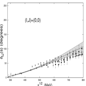
Figure 11: Standard NLO-ChPT phase shifts (in degrees) for $\pi\pi$ scattering for $S-$ and $P-$ waves after Eq. (10). Upper panel: Set Ic of Ref. [23]. Lower panel: Set III of Ref. [23].Combined data from Refs. [2]-[10].

Figure 12: NLO-IAM Unitarized phase shifts (in degrees) for $\pi\pi$ scattering for $S-$ and $P-$ waves. Monte Carlo scheme (see main text). Upper panel: Set Ic of Ref. [23]. Lower panel: Set III of Ref. [23]. Combined data from Refs. [2]-[10].

Figure 13: NLO-IAM Unitarized phase shifts (in degrees) for $\pi\pi$ scattering for $S-$ and $P-$ waves. Partial fit scheme (see main text). The errors in the curves are due to uncertainties in $\bar{l}_{3}$ and $\bar{l}_{4}$. Combined data from Refs. [2]-[10].

4 On the convergence of the IAM method

The IAM method can be systematically implemented to any order in the chiral expansion with no additional LEC’s than those required by standard ChPT. There arises the question to what extent is this method convergent. To answer this question in practice we can only compare one-loop and two loop predictions for the unitarized phase shifts. Such a comparison makes sense only if errors in the LECS are also transported, as we have repeatedly done along this work. Actually, in Ref. [29] the one loop error analysis of the IAM phase shifts was estimated by varying the low energy constants. In this section we reanalyze this question by using the updated values of the one loop coefficients given by Set Ic and Set III taking into account by means of a Monte-Carlo simulation the important anticorrelations between $\bar{l}_{1}$ and $\bar{l}_{2}$ determined in Ref. [23]. Following the same systematics of the two loop calculation, we show in Fig. 10 the unitarity condition of Eq. (9). As one would expect, unitarity violations of one-loop ChPT occurr at lower energies. The NLO ChPT phase shifts, defined through Eq. (10) are depicted in Fig. 11. The general trend follows a similar pattern to the two loop calculation, although some important differences emerge. Firstly, the uncertainties in the phase shifts are smaller at NNLO than at NLO in the threshold region, as one would expect from the fact that threshold parameters are more accurately determined at NNLO than at NLO [23]. In the region above threshold the situation is exactly the opposite, the two loop calculation produces larger uncertainties than the one loop one. In addition, by comparison of Fig. 11 and Figs. 2 and (4 in the $\rho$ channel) one sees that the discrepances in the region above threshold are larger than the estimated uncertainties, with an overall trend to improvement in the two loop calculation. A similar trend, although in a less clear manner, is observed in the two $S-$waves. The unitarity condition, Eq. (9), gives us a good idea on the applicability of standard ChPT to one and two loop approximations. Nevertheless, the agreement of the perturbative phase shifts, Eq. (10), with experiment seems to extend up to a region where the unitarity violation may be as large as $10-20\%$.

The one loop IAM phase shifts are depicted in Fig. 12. Apparently, the general picture provided by NLO-ChPT looks better than what one obtains by comparing any of the two Monte-Carlo schemes studied in Sect. 3 based in NNLO-ChPT. By looking at any of these two-loop schemes, Fig. 6 and Fig. 7, we realize that there is a clear loss of predictive power; the errors in the two loop phase shifts are larger than the discrepancy between their mean value and the one loop mean value. Finally, in Fig. 13 a partial one-loop fit procedure in $\bar{l}_{1}$ and $\bar{l}_{2}$ parameters to the data is presented, where variations on the $\bar{l}_{3}$ and $\bar{l}_{4}$ are taken into account. The result of the fit is

$$\bar{l}_{1}=-0.44\pm 0.02\qquad\bar{l}_{2}=5.51\pm 0.04\qquad r(\bar{l}_{1},\bar{l}_{2})=-0.81$$ (31)

where the errors reflect the uncertainites in $\bar{l}_{3}$ and $\bar{l}_{4}$. Here $\chi^{2}/{\rm d.o.f.}=191/(67-2)=2.94$ almost three times larger than in the two loops case (1.11), and too large to be considered a satisfactory drescription of the scattering data. Such a large $\chi^{2}$ value makes the determination of the uncertainties of $\bar{l}_{1}$ and $\bar{l}_{2}$ due to the error bars in the fitted data meaningless. As we see, the obtained values for the fitted parameters are compatible with the corresponding two loop partial fit procedure, Eq. (21), although the errors in the one-loop case due to uncertainties in $\bar{l}_{3}$ and $\bar{l}_{4}$ are much smaller than in the two-loop case. This may be an indirect consequence of the large $\chi^{2}$ value.

5 Conclusions

In the present work we have presented a thorough study of the Inverse Amplitude Method to unitarize the NLO (one-loop) and NNLO (two-loop) ChPT $\pi\pi$ scattering amplitudes below the $K\bar{K}$ threshold. To this end, we have considered several one-loop $\bar{l}_{1,2,3,4}$ and two loop $\bar{b}_{1,2,3,4,5,6}$ parameter sets along the lines discussed in our previous work [23]. Particularly interesting in this work is the role played by the uncertainties in these parameters. To complement the analysis and provide some quantitative motivation we have determined unitarity violations within standard ChPT, with error estimates. They take place at much lower energies than the unitarity limit suggests. Moreover, we have also shown the systematic discrepancy with the data in the region above threshold if phase shifts are defined perturbatively. The discussion is complicated by the fact that the two loop parameters $\bar{b}_{1,2,3,4,5,6}$ may by splitted in a zeroth order contribution $\bar{b}_{1,2,3,4,5,6}^{0}$ and a higher order contribution $\Delta\bar{b}_{1,2,3,4,5,6}$ which slightly spoils the chiral counting. The distinction caused in the phase shifts by including or not the higher contribution is small within ChPT. Motivated by this we have unitarized the two loop amplitude, and devised several schemes to predict the phase-shifts from threshold up to the resonance region. The effect of consistently treating or not $\Delta\bar{b}_{1,2,3,4,5,6}$ as higher order is much stronger for the IAM unitarized phase shifts. Typically, a factor of two difference or larger in the uncertainties is encountered. In any case, they are rather large, although seem consistent with the scattering data. This indicates a kind of fine tuning going on and suggests a fit to the data to determine the low energy parameters which remain in the chiral limit, keeping the remaining low energy parameters within their error bars. The result of the fit is satisfactory, although there appears a discrepancy in the $\bar{b}_{6}$ coefficient. Nevertheless, the predicted partially fitted phase shifts vary within very small uncertainties, not far from the recent ChPT analysis of Roy equations carried out in Ref. [42]. Despite of these features, the IAM produces crossing violations which have been quantified in terms of Roskies sume rules. Generally speaking, they are not very large in percentage terms, although in some cases the uncertainties are so large that no conclusion can be drawn. We have also studied some proposals to generalize the IAM in order to achieve a better fulfillment of crossing properties. Finally, we have adressed the convergence of an expansion based on the IAM and increasing order of approximation in ChPT. By comparing NLO (one-loop) and NNLO (two-loop) IAM predicted phase shifts we see at the present stage a lack of predictive power; the errors in the two loop phase-shift are larger than the difference between the central one-loop and two-loop values. This is a direct consequence of the low accuracy in the two loop parameters.

Appendix A Correlations among NNLO low energy constants and threshold parameters in standard ChPT

The correlation matrix, defined as usual,

$$r_{ij} = \langle x_{i}x_{j}\rangle$$

$$x_{i} = \frac{c_{i}-\langle c_{i}\rangle}{\sqrt{\langle c_{i}^{2}\rangle-\langle c_{i}\rangle^{2}}}$$

$$\langle f(c_{1},\dots,c_{n})\rangle = \frac{1}{N}\sum_{\alpha=1}^{N}f(c_{1,\alpha},\dots,c_{n,\alpha})$$ (32)

being $c_{i}$ any of the low energy constants or threshold parameters is provided below as obtained from our $N=10^{4}$ finite size samples both for Set Ic and Set III. Taking into account the central values and their errors given in Table 2 and Table 6 and ignoring the slight error asymmetries the parameter Sets are fully portable by going through diagonalization to principal axis in parameter space and making a Monte-Carlo Gaussian simulation in each principal direction.

Set Ic

$$r(\bar{b}_{i},\bar{b}_{j}) = \left(\matrix{+1.00&&&&&\cr-0.74&+1.00&&&&\cr+0.53&-0.77&+1.00&&&\cr-0.49&+0.64&-0.49&+1.00&&\cr+0.09&+0.04&-0.41&+0.10&+1.00&\cr-0.08&+0.23&-0.54&+0.23&+0.57&+1.00}\right)$$

$$\matrix{\qquad a_{00}&\quad a_{11}&\quad a_{20}&\quad b_{00}&\quad b_{11}&\quad b_{20}}$$

$$r_{ij}^{\rm Threshold} = \left(\matrix{+1.00&&&&&\cr+0.13&+1.00&&&&\cr+0.58&-0.21&+1.00&&&\cr+0.75&-0.13&+0.37&+1.00&&\cr+0.02&+0.89&-0.07&-0.10&+1.00&\cr+0.20&+0.06&+0.57&+0.38&+0.11&+1.00}\right)$$ (34)

Set III

$$r(\bar{b}_{i},\bar{b}_{j}) = \left(\matrix{+1.00&&&&&\cr-0.73&+1.00&&&&\cr+0.53&-0.76&+1.00&&&\cr-0.12&+0.20&-0.14&+1.00&&\cr+0.22&-0.16&-0.19&+0.21&+1.00&\cr+0.06&+0.02&-0.29&+0.19&+0.47&+1.00}\right)$$

$$\matrix{\qquad a_{00}&\quad a_{11}&\quad a_{20}&\quad b_{00}&\quad b_{11}&\quad b_{20}}$$

$$r_{ij}^{\rm Threshold} = \left(\matrix{+1.00&&&&&\cr-0.08&+1.00&&&&\cr+0.67&-0.46&+1.00&&&\cr+0.81&-0.32&+0.55&+1.00&&\cr-0.11&+0.82&-0.23&-0.18&+1.00&\cr+0.37&-0.45&+0.71&+0.59&-0.21&+1.00\cr}\right)$$ (36)

References

• [1] S.M. Roy; Phys. Lett. B 36 (1971) 353.
• [2] S. D. Protopopescu et. al., Phys. Rev. D7 (1973) 1279.
• [3] B. Hyams, et al., Nucl. Phys. B 64 (1973) 134; W. Ochs, Thesis, Ludwig-Maximilians-UniversitΓ€t, 1973.
• [4] P. Estabrooks and A. D. Martin, Nucl. Phys. B79 (1974) 301.
• [5] M. J. Losty et al., Nucl. Phys. B69 (1974) 185.
• [6] V. Srinivasan et. al., Phys. Rev. D12 (1975) 681.
• [7] L. Rosselet et. al., Phys. Rev. D15 (1977) 574.
• [8] R. Kaminski, L. Lesniak and K. Rybicki, Z. Phys. C74 (1997)79.
• [9] W. Hoogland et. al., Nucl. Phys. B126 (1977) 109.
• [10] C.D. Froggatt and J.L.Petersen, Nucl. Phys. B129 (1977) 89.
• [11] S. Weinberg, Phys. Rev. Lett 17 (1966) 616,
• [12] J. Gasser and H. Leutwyler, Ann. Phys. (N.Y.) 158 (1984) 142.
• [13] J. Gasser and H. Leutwyler, Nucl. Phys. B250 (1985) 465.
• [14] M. Knecht, B. Moussallam, J. Stern and N.H. Fuchs, Nucl. Phys. B457 (1995)513; ibidem B471 (1996)445;
• [15] J. Bijnens, G. Colangelo, G. Ecker, J. Gasser and M.E. Sainio, Phys. Lett. B374 (1996) 210; ibid. Nucl. Phys. B508 (1997) 263. Erratum ibid . B 517 (1998) 639
• [16] G. Ecker, J. Gasser, A. Pich and E. de Rafael, Nucl. Phys. B321 (1989) 311.
• [17] L. Girlanda, M. Knecht, B. Moussallam an J. Stern, Phys. Lett. B 409 (1997) 461.
• [18] J. Bijnens, G. Colangelo and J. Gasser, Nucl. Phys. B 427 (1994) 427.
• [19] G. Amoros, J. Bijnens and P. Talavera; Phys. Lett. B 480 (2000) 71.
• [20] G. Amoros, J. Bijnens and P. Talavera, Nucl.Phys. B 585 (2000); Erratum ibid. B 598 (2001)665.
• [21] J. Bijnens, G. Colangelo and P. Talavera, JHEP 9805 (1998) 014.
• [22] O. Dumbrajs et al., Nucl. Phys. B 216 (1983) 277.
• [23] J. Nieves and E. Ruiz Arriola, Eur. Jour. Phys. A 8 (2000) 377.
• [24] Tran N. Truong, Phys. Rev. Lett. 61 (1988) 2526.
• [25] A. Dobado, M.J. Herrero and T.N. Truong, Phys. Lett. B235 (1990) 134.
• [26] Tran N. Truong, Phys. Rev. Lett. 67( 1991) 2260.
• [27] A. Dobado and J. R. PelΓ‘ez; Phys. Rev. D 47(1993) 4883.
• [28] T. Hannah, Phys. Rev. D 54 (1996) 4648.
• [29] A. Dobado and J.R. Pelaez; Phys. Rev. D 56 (1997) 3057.
• [30] M. Boglione and M.R. Pennington, Z. Phys. C 75 (1997) 113.
• [31] T. Hannah, Phys. Rev. D 55 (1997) 5613.
• [32] J.A. Oller, E. Oset and J.R. Pelaez, Phys. Rev. Lett. 80 (1998) 3452; Phys.Rev. D 59 (1999) 074001, Erratum-ibid. D 60 (1999) 099906.
• [33] A. GΓ³mez Nicola and J. R. PelΓ‘ez, hep-ph/010956
• [34] T. Hannah, Phys. Rev. D 59 (1999) 057502.
• [35] J. Nieves and E. Ruiz Arriola, Phys. Lett. B455 (1999) 30.
• [36] J. Nieves and E. Ruiz Arriola, Nucl. Phys. A 679 (2000) 57.
• [37] E. Ruiz Arriola, A. Gomez Nicola, J. Nieves and J.R. Pelaez; Talk given at Miniworkshop Bled 2000: Few Quark Problems, Bled, Slovenia, 8-15 Jul 2000; hep-ph/0011164
• [38] R. Roskies, Nuovo Cimento 65 A (1970)
• [39] C. S. Cooper and M. R. Pennington, J. Math. Phys. 12 /1971) 1509.
• [40] I. P. Cavalcante and J. Sa Borges; hep-ph/0101037
• [41] B. Ananthanarayan, G. Colangelo, J. Gasser and H. Leutwyler, hep-ph/0005297 and references therein.
• [42] G. Colangelo, J. Gasser and H. Leutwyler; hep-ph/0103088
• [43] T. Becher and H. Leutwyler, JHEP 06 (2001) 017.