Unitarization of the complete meson-meson scattering at one loop in Chiral Perturbation Theory.

Abstract

We report on our one-loop calculation of all the two meson scattering amplitudes within SU(3) Chiral Perturbation Theory, i.e. with pions, kaons and etas. Once the amplitudes are unitarized with the coupled channel Inverse Amplitude Method, they satisfy simultaneously the correct low-energy chiral constraints and unitarity. We obtain a remarkable description of meson-meson scattering data up to 1.2 GeV including the scattering lengths and seven light resonances.

A Introduction

Chiral Perturbation Theory (ChPT) [1] provides a powerful tool to describe the interactions of the lightest mesons. These particles correspond to the Goldstone bosons associated to the spontaneous breaking of the $SU(3)_{L}\times SU(3)_{R}$ chiral symmetry down to $SU(3)_{L+R}$. This would be the symmetry breaking pattern of QCD if the three lightest quarks were massless. Of course, quarks are not massless, but since their masses are very small compared to the typical hadronic scales, ${\cal O}$(1 GeV), their explicit symmetry breaking effect only yields a small mass contribution for the lightest mesons, which become pseudo-Goldstone bosons. Thus, the three pions are the pseudo-Goldstone bosons of the $SU(2)$ spontaneous breaking when only the $u$ and $d$ quarks are considered. Similarly, when $s$ is also included, the eight $SU(3)$ pseudo-Goldstone bosons can be identified with the meson octet formed by the pions, kaons and the eta.

The low energy interactions of pions, kaons and the eta have to be described with an effective Lagrangian respecting the above described chiral symmetry breaking pattern. Within ChPT, only pseudo-Goldstone bosons are included in the Lagrangian, thus providing a low energy description. The possible terms compatible with the symmetry breaking pattern are organized in a derivative and mass expansion (generically $p$). For instance, amplitudes are obtained as an expansion in powers of the external momenta and the quark masses over a typical chiral scale of ${\cal O}$(1 GeV). One remarkable feature of the ChPT scheme is that all loop divergences appearing at a given order in the expansion can be absorbed by a finite number of (low energy) constants of the counterterms that appear in the Lagrangian to the same order. Therefore, order by order, the theory is finite and depends on a few parameters, providing a predictive framework. Thus, once the low-energy constants are determined from just a few experiments, predictions can be made for other processes.

This approach is very successful, but only at low energies (usually, less than 500 MeV). For that reason, there is a growing interest in developing methods to extend the ChPT applicability range. Among them, the explicit introduction of heavier resonances in the Lagrangian [2], resummation of diagrams in a Lippmann-Schwinger or Bethe-Salpeter approach [3], or unitarization and dispersive techniques like the Inverse Amplitude Method (IAM) [4, 5] applied to one-loop amplitudes. A version of the latter, generalized to coupled channels provided a remarkable description of meson-meson scattering up to 1.2 GeV, generating dynamically seven light resonances [6].

In principle, these methods respect the good low energy properties of ChPT, since they are built from the perturbative results. However, not all the meson-meson scattering processes had been calculated at one loop in ChPT. The amplitudes available so far are $\pi\pi\rightarrow\pi\pi$ [7], $K\pi\rightarrow K\pi$ [7], $\eta\pi\rightarrow\eta\pi$ [7] and the two independent $K^{+}K^{-}\rightarrow K^{+}K^{-}$, $K^{+}K^{-}\rightarrow K^{0}\bar{K}^{0}$ [8]. Therefore, the IAM has only been applied rigorously to the $\pi\pi$, $K\bar{K}$ final states, whereas for the complete low-energy meson-meson scattering, additional approximations had to be done [6], meaning in particular that it was not possible to compare with the low energy parameters of standard ChPT in dimensional regularization or to describe simultaneously the low and high energy regimes.

Here we report on our recent work [9] where we have completed the calculation of the meson-meson scattering in one-loop ChPT. There are three completely new amplitudes: $K\eta\rightarrow K\eta$, $\eta\eta\rightarrow\eta\eta$ and $K\pi\rightarrow K\eta$. In addition, we have recalculated independently the other five amplitudes and all of them will be given together in a unified notation, ensuring exact perturbative unitarity and also correcting some misprints in the literature.

Once all the amplitudes are available, we have done a coupled channel IAM fit to describe the whole meson-meson scattering data below 1.2 GeV. Our results allow for a direct comparison with the standard low-energy chiral parameters. Indeed, we find a very good agreement with previous determinations from low-energy data using standard ChPT. The main differences of our work with [6] are that we consider the full one-loop calculation of the amplitudes, which ensures their finiteness and scale independence in dimensional regularization, we take into account the new processes mentioned above and we are able to describe simultaneously the low energy and the resonance regions.

B The amplitudes

The lowest order, ${\cal O}(p^{2})$, meson-meson scattering amplitudes (the low energy theorems) are obtained just from the tree level diagrams of the lowest order Lagrangian. In contrast, the calculation of the ${\cal O}(p^{4})$ contribution involves the evaluation of the following Feynman diagrams: First, the one-loop diagrams in Fig.1, which are divergent. In particular those in Fig.1e, provide the wave function, mass and decay constant renormalizations, and that in Fig.1a gives the imaginary part to ensure perturbative unitarity. Second, the tree level graphs with the second order Lagrangian, which depend on the chiral parameters $L_{i}$, that will absorb the previous divergences through renormalization. In Table I, we list the $L_{i}$ values from recent determinations. Note that the parameters have been renormalized in the usual $\overline{MS}-1$ scheme of ChPT, using dimensional regularization. Thus, the renormalized parameters have a scale dependence $L_{i}^{r}(\mu)$ (except $L_{3}$ and $L_{7}$), and they are given at $\mu=M_{\rho}$.

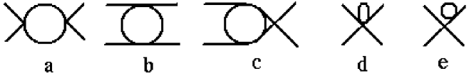
FIG. 1.: Generic one-loop Feynman diagrams that have to be evaluated in meson-meson scattering.

Chiral Parameter	${\cal O}(p^{6})$ $K_{l4}$ decays	${\cal O}(p^{4})$ $K_{l4}$ decays	ChPT	IAM fits
$L_{1}^{r}(M_{\rho})$	$0.53\pm 0.25$	$0.46$	$0.4\pm 0.3$	$0.56\pm 0.10$
$L_{2}^{r}(M_{\rho})$	$0.71\pm 0.27$	$1.49$	$1.35\pm 0.3$	$1.21\pm 0.10$
$L_{3}$	$-2.72\pm 1.12$	$-3.18$	$-3.5\pm 1.1$	$-2.79\pm 0.14$
$L_{4}^{r}(M_{\rho})$	0	0	$-0.3\pm 0.5$	$-0.36\pm 0.17$
$L_{5}^{r}(M_{\rho})$	$0.91\pm 0.15$	$1.46$	$1.4\pm 0.5$	$1.4\pm 0.5$
$L_{6}^{r}(M_{\rho})$	0	0	$-0.2\pm 0.3$	$0.07\pm 0.08$
$L_{7}$	$-0.32\pm 0.15$	$-0.49$	$-0.4\pm 0.2$	$-0.44\pm 0.15$
$L_{8}^{r}(M_{\rho})$	$0.62\pm 0.2$	$1.00$	$0.9\pm 0.3$	$0.78\pm 0.18$

TABLE I.: Different sets of chiral parameters ($\times 10^{3}$). The first two columns come from recent analysis of $K_{l4}$ decays at different orders [10] ($L_{4}$ and $L_{6}$ are set to zero). In the third column $L_{1},L_{2},L_{3}$ come from [11] and the rest from [1]. The last one corresponds to the values from the IAM including the uncertainty due to different systematic error used on different fits.

After renormalization, the amplitudes are finite and scale independent. The details and results of the calculation will be published elsewhere [9]. We will just recall that, in order to compare with experiment, the amplitudes are projected into partial waves $t_{IJ}$ of definite isospin $I$ and angular momentum $J$. Therefore, in the chiral expansion we will have, omitting the $I,J$ subindices, $t\simeq t_{2}+t_{4}+...$, where $t_{2}$ and $t_{4}$ the ${\cal O}(p^{2})$ and ${\cal O}(p^{4})$ contributions, respectively.

C Unitarity

The $S$ matrix unitarity relation $SS^{\dagger}=1$ translates into simple relations for the elements of the $T$ matrix $t_{ij}$ if they are projected into partial waves, where $i,j$ denote the different states physically available. For instance, if there is only one possible state, ”1”, the partial wave $t_{11}$ satisfies

$${\mbox{Im}\,}t_{11}=\sigma_{1}\,|\,t_{11}|^{2}\quad\Rightarrow\quad{\mbox{Im}\,}\frac{1}{t_{11}}=-\sigma_{1}\quad\Rightarrow\quad t_{11}=\frac{1}{{\mbox{Re}\,}t_{11}-i\,\sigma_{1}}$$ (1)

where $\sigma_{i}=2q_{i}/\sqrt{s}$ and $q_{i}$ is the C.M. momentum of the state $i$. Written in this way it can be readily noted that we only need to know the real part of the Inverse Amplitude. The imaginary part is fixed by unitarity. In principle, this relation only holds above threshold up to the energy where another state, ”2”, is physically accessible. Above that point, the unitarity relation for the partial waves can be written in matrix form as:

$${\mbox{Im}\,}T=T\,\Sigma\,T^{*}\quad\Rightarrow\quad{\mbox{Im}\,}T^{-1}=-\Sigma\quad\Rightarrow\quad T=({\mbox{Re}\,}T-i\,\Sigma)^{-1}$$ (2)

with

$$T=\left(\begin{array}[]{cc}t_{11}&t_{12}\\ t_{12}&t_{22}\\ \end{array}\right)\quad,\quad\Sigma=\left(\begin{array}[]{cc}\sigma_{1}&0\\ 0&\sigma_{2}\\ \end{array}\right)\,,$$ (3)

which allows for an straightforward generalization to the case of $n$ accessible states. Once more, unitarity means that we would only need to calculate the real part of the inverse amplitude matrix.

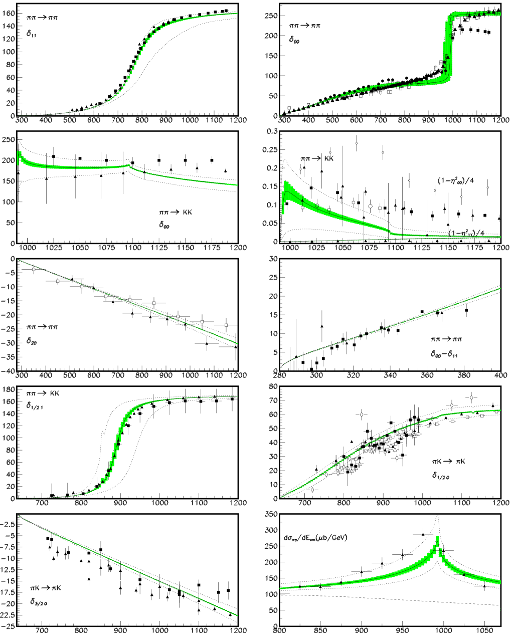
FIG. 2.: Result of the coupled channel IAM fit to meson-meson scattering data (see [9] for references). The shaded area covers the uncertainty due to MINUIT errors. The area between the dotted lines corresponds to the uncertainty in the $L^{r}_{i}$ due to the use of different systematic errors on the fits. The dashed line in the last plot is the continuous background underneath the resonant contribution.

Note that the above unitarity relations are non-linear. This implies that they will never be satisfied exactly with polynomials like the amplitudes obtained from ChPT. Nevertheless, unitarity holds perturbatively, i.e,

$${\mbox{Im}\,}T_{2}=0+{\cal O}(p^{4}),\quad\quad{\mbox{Im}\,}T_{4}=T_{2}\,\Sigma\,T_{2}^{*}\,+{\cal O}(p^{6}),$$ (4)

D Unitarization: The inverse Amplitude Method

One of the simplest methods to unitarize the chiral amplitudes is to introduce the ${\mbox{Re}\,}T$ in eq.(2), calculated as a ChPT expansion

$$T^{-1} \simeq T_{2}^{-1}(1-T_{4}T_{2}^{-1}+...),$$ (5)

$${\mbox{Re}\,}T^{-1} \simeq T_{2}^{-1}(1-({\mbox{Re}\,}T_{4})T_{2}^{-1}+...),$$ (6)

Taking into account the perturbative unitarity conditions, eq.(4), we find

$$T\simeq T_{2}(T_{2}-T_{4})^{-1}T_{2},$$ (7)

which is the coupled channel Inverse Amplitude Method, which will use to unitarize simultaneously all the one-loop ChPT meson-meson scattering amplitudes. This method is able to generate seven resonant states. The novelty of our approach is that, since we have the complete ${\cal O}(p^{4})$ ChPT amplitudes, we can simultaneously recover the very same ChPT amplitudes up to ${\cal O}(p^{4})$, and thus have a good low energy limit.

E Results and conclusion

We can now use previous determinations of the chiral parameters with the IAM and even the correct resonant behavior resonances. Once more, we can use the $L_{i}^{r}$ because we have the complete amplitudes renormalized in the $\bar{MS}-1$ scheme. We have nevertheless carried out a fit (using MINUIT [12]) of the presently available data on meson-meson scattering. Since there are incompatibilities between different experiments, customarily a $1\%$, $3\%$ and $5\%$ systematic error has been added, which introduces an additional source of error. We give in Table 1 the resulting chiral parameters from the fit, whose errors correspond to those of MINUIT combined with those from the systematic uncertainty. Note that they are compatible with previous determinations.

In Fig.2 we show the results of the IAM fit to these data, which is given in terms of phase shifts, inelasticities, and mass distributions of different processes (see [9] for details). The gray error bands cover the uncertainties in the $L_{i}$ due to MINUIT, and are calculated by a Monte-Carlo gaussian sampling of the parameters. The area between the dotted lines has been calculated similarly but with the errors in the chiral parameters due to the different choice of systematic error. It can be noticed that all the resonant features are reproduced. However, thanks to the new amplitudes we are also able to obtain simultaneously values for the threshold parameters (they have not been fitted) which are listed in table 2. Note the good agreement with the experimental values when they exist.

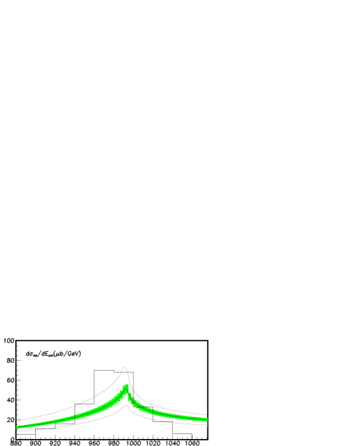
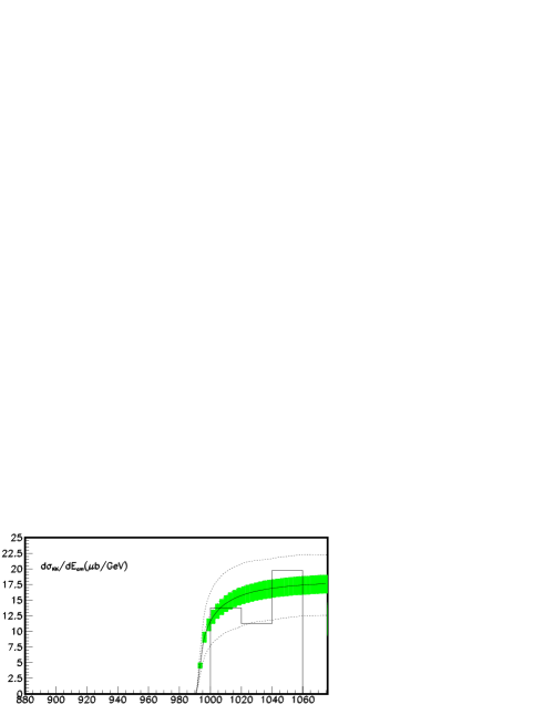
FIG. 3.: Effective mass distributions of the two mesons in the final state of $K^{-}p\rightarrow\Sigma^{+}(1385)\pi\eta$ and $K^{-}p\rightarrow\Sigma^{+}(1385)K\bar{K}$. This plots are not part of the IAM fit. For data references see [9].

Threshold	Experiment	IAM fit	ChPT ${\cal O}(p^{4})$	ChPT ${\cal O}(p^{6})$
parameter			[2, 5, 7]	[13]
$a_{0\,0}$	0.26 $\pm$0.05	0.231${}^{+0.003}_{-0.006}$	0.20	0.219$\pm$0.005
$b_{0\,0}$	0.25 $\pm$0.03	0.30$\pm$ 0.01	0.26	0.279$\pm$0.011
$a_{2\,0}$	-0.028$\pm$0.012	-0.0411${}^{+0.0009}_{-0.001}$	-0.042	-0.042$\pm$0.01
$b_{2\,0}$	-0.082$\pm$0.008	-0.074$\pm$0.001	-0.070	-0.0756$\pm$0.0021
$a_{1\,1}$	0.038$\pm$0.002	0.0377$\pm$0.0007	0.037	0.0378$\pm$0.0021
$a_{1/2\,0}$	0.13…0.24	0.11${}^{+0.06}_{-0.09}$	0.17
$a_{3/2\,0}$	-0.13…-0.05	-0.049${}^{+0.002}_{-0.003}$	-0.5
$a_{1/2\,1}$	0.017…0.018	0.016$\pm$0.002	0.014
$a_{1\,0}$		0.15${}^{+0.07}_{-0.11}$	0.0072

TABLE II.: Scattering lengths $a_{I\,J}$ and slope parameters $b_{I\,J}$ for different meson-meson scattering channels. For experimental references see [9]. Let us remark that our one-loop IAM results are very similar to those of two-loop ChPT.

REFERENCES

- [1] S. Weinberg, Physica A96, (1979) 327. J. Gasser and H. Leutwyler, Ann. Phys. 158, (1984) 142. J. Gasser and H. Leutwyler, Nucl. Phys. B250, (1985) 465,517,539.
- [2] V. Bernard, N. Kaiser and U.G. Meißner, Nucl. Phys. B364 (1991), 283. J.A. Oller, E. Oset, Phys.Rev.D60:074023,1999. M.Jamin, J.A. Oller, A.Pich, Nucl.Phys.B587 (2000), 331-362.
- [3] J.A. Oller, and E. Oset Nucl. Phys. A620 (1997), 438. J. Nieves, E. Ruiz Arriola. Phys.Rev.D63 (2001) 076001.
- [4] T. N. Truong, Phys. Rev. Lett. 661, (1988) 2526 ;Phys. Rev. Lett. 67, (1991) 2260; A. Dobado, M.J.Herrero and T.N. Truong, Phys. Lett. B235, (1990) 134;
- [5] A. Dobado and J.R. Peláez, Phys. Rev. D47, (1993) 4883; Phys. Rev. D56, (1997) 3057.
- [6] J. A. Oller, E. Oset and J. R. Peláez, Phys. Rev. Lett. 80, (1998) 3452; Phys. Rev. D59, (1999) 074001; Erratum-ibid. D60, (1999) 099906.
- [7] V. Bernard, N. Kaiser, U.G. Meissner, Phys. Rev. D43 (1991), 2757; Nucl. Phys. B357 (1991), 129; Phys. Rev. D44 (1991), 3698.
- [8] F. Guerrero and J. A. Oller, Nucl. Phys. B537, (1999) 459.
- [9] A. Gómez Nicola and J. R. Peláez, hep-ph/0109056.
- [10] G. Amorós, J. Bijnens and P. Talavera, Nucl. Phys. B602(2001),87.
- [11] J. Bijnens, G. Colangelo and J. Gasser, Nucl. Phys. B427, (1994) 427.
- [12] F. James, Minuit Reference Manual D506 (1994).
- [13] G. Amorós, J. Bijnens and P. Talavera, Nucl.Phys.B585:293-352,2000, Erratum-ibid.B598:665-666,2001.