FSU-HEP-2001-0602

BNL-HET-01/19

UR-1639

hep-ph/0109066

QCD Corrections to Associated

$t\bar{t}h$ Production at the Tevatron

L. Reina
Physics Department, Florida State University,
Tallahassee, FL 32306-4350, USA

S. Dawson
Physics Department, Brookhaven National Laboratory,
Upton, NY 11973, USA

D. Wackeroth
Department of Physics and Astronomy, University of Rochester,
Rochester, NY 14627-0171, USA

We present in detail the calculation of the ${\cal O}(\alpha_{s}^{3})$ inclusive total cross section for the process $p{\overline{p}}\rightarrow t{\overline{t}}h$ in the Standard Model, at the Tevatron center-of-mass energy $\sqrt{s_{\scriptscriptstyle H}}\!=\!2$ TeV. The next-to-leading order QCD corrections significantly reduce the renormalization and factorization scale dependence of the Born cross section. They slightly decrease or increase the Born cross section depending on the values of the renormalization and factorization scales.

1 Introduction

Among the most important goals of present and future colliders is the study of the electroweak symmetry breaking mechanism and the origin of fermion masses. If the introduction of one or more Higgs fields is responsible for the breaking of the electroweak symmetry, then at least one Higgs boson should be relatively light, and certainly in the range of energies of present (Tevatron) or future (LHC) hadron colliders. The present lower bounds on the Higgs boson mass from direct searches at LEP2 are $M_{h}\!>\!114.1$ GeV (at $95\%$ CL) [1] for the Standard Model (SM) Higgs boson, and $M_{h^{0}}\!>\!91.0$ GeV and $M_{A^{0}}\!>\!91.9$ GeV (at $95\%$ CL, $0.5\!<\!\tan\beta\!<\!2.4$ excluded) [2] for the light scalar ($h^{0}$) and pseudoscalar ($A^{0}$) Higgs bosons of the minimal supersymmetric standard model (MSSM). At the same time, global SM fits to all available electroweak precision data indirectly point to the existence of a light Higgs boson, $M_{h}\!<\!212-236$ GeV [3], while the MSSM requires the existence of a scalar Higgs boson lighter than about 130 GeV [4]. Therefore, the possibility of a Higgs boson discovery in the mass range around 115-130 GeV seems increasingly likely.

In this context, the Tevatron will play a crucial role and can potentially discover a Higgs boson in the mass range between the present experimental lower bound and about 180 GeV [5]. The dominant Higgs production modes at the Tevatron are gluon-gluon fusion ($gg\rightarrow h$) and the associated production with a weak boson ($q\bar{q}\rightarrow Wh,~{}Zh$). Because of small event rates and large backgrounds, the Higgs boson search in these channels is extremely difficult, requiring the highest possible luminosity. It is therefore important to investigate all possible production channels, in the effort to fully exploit the range of opportunities offered by the available statistics.

Recently, attention has been drawn to the possibility of detecting a Higgs signal in association with a pair of top-antitop quarks at the Tevatron, i.e. in $p\bar{p}\rightarrow t\bar{t}h$ [6]. This production mode can play a role over most of the Higgs mass range accessible at the Tevatron. Although it has a small event rate, $\sim 1-5$ fb for a SM-like Higgs boson, and even lower for an MSSM Higgs boson, the signature ($W^{+}W^{-}b\bar{b}b\bar{b}$) is quite spectacular. Furthermore, at the Tevatron, after fully reconstructing both top quarks, the shape of the invariant mass distribution of the remaining $b{\overline{b}}$ pair is quite different for the signal and for the background. The statistics is too low to allow any direct measurement of the top-quark Yukawa coupling, but recent studies [7] indicate that this channel can reduce the luminosity required for the discovery of a SM-like Higgs boson at Run II of the Tevatron by as much as 15-20%.

The total cross section for $p\bar{p}\rightarrow t\bar{t}h$ has been known at tree-level for quite some time [8]. As for any other hadronic process, next-to-leading (NLO) QCD corrections are expected to be important and are crucial in order to reduce the dependence of the cross section on the renormalization and factorization scales. Preliminary indications of the magnitude of the NLO QCD corrections can be obtained in the framework of the Effective Higgs Approximation (EHA), where terms of order $M_{h}/\sqrt{s}$ and $M_{h}/m_{t}$ are systematically neglected in the computation [9]. This approximation correctly reproduces the collinear bremsstrahlung of the Higgs boson from the heavy top quarks. However, we expect the EHA to be more reliable at the LHC center-of-mass energies, for which it was originally proposed, than at the Tevatron center-of-mass energies. We will briefly discuss the predictions of the EHA for $p\bar{p}\rightarrow t\bar{t}h$ in Sec. 6.

We also notice that QCD corrections to the associated production of a Higgs boson with a pair of $b\bar{b}$ quarks, which is dominated by the $gg\rightarrow b\bar{b}h$ channel, have been computed in the limit of large $M_{h}$ [10], by resuming the leading $\ln(M_{h}/m_{b})$ terms. However this result cannot be applied to the $t{\overline{t}}h$ production of a relatively light Higgs boson at the Tevatron, both because the ratio $M_{h}/m_{t}$ is of ${\cal O}(1)$ and does not justify the large $M_{h}$ limit, and because the $gg$ channel is negligible for $t\bar{t}h$ production at the Tevatron.

In this paper we present in detail the calculation of the NLO inclusive total cross section for $p\bar{p}\rightarrow t\bar{t}h$, $\sigma_{\scriptscriptstyle NLO}(p\bar{p}\rightarrow t\bar{t}h)$, in the Standard Model, at the Tevatron center-of-mass energy. For $p{\overline{p}}$ collisions at hadronic center-of-mass energy $\sqrt{s_{\scriptscriptstyle H}}\!=\!2$ TeV, more than $95\%$ of the tree-level cross section comes from the sub-process $q\bar{q}\rightarrow t\bar{t}h$. Therefore, we include only the $q\bar{q}\rightarrow t\bar{t}h$ channel when computing the tree-level total cross section, and we calculate the NLO total cross section by adding the complete set of virtual and real ${\cal O}(\alpha_{s})$ corrections to $q\bar{q}\rightarrow t\bar{t}h$. The Feynman diagrams contributing to $q\bar{q}\rightarrow t\bar{t}h$ at lowest order are shown in Fig. 1, while examples of ${\cal O}(\alpha_{s})$ virtual and real corrections are given in Figs. 2-6. The main challenge in the calculation of the ${\cal O}(\alpha_{s})$ virtual corrections comes from the presence of pentagon diagrams with several massive external and internal particles. We have calculated the corresponding pentagon scalar integrals as linear combinations of scalar box integrals using the method of Ref. [11]. The real corrections are computed using the phase space slicing method, in both the double [12, 13] and single [14, 15, 16] cutoff approach. This is the first application of the single cutoff phase space slicing approach to a cross section involving more than one massive particle in the final state.

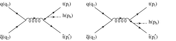
Figure 1: Feynman diagrams contributing to the lowest order process, $q\bar{q}\rightarrow t\bar{t}h$. The arrows indicate the momentum flow.

Numerical results for our calculation of $\sigma_{\scriptscriptstyle NLO}(p\bar{p}\rightarrow t\bar{t}h)$ at the hadronic center-of-mass energy $\sqrt{s_{\scriptscriptstyle H}}\!=\!2$ TeV have been presented in [17]. An independent calculation of the NLO total cross section for $p\bar{p}\rightarrow t\bar{t}h$ has been performed by Beenakker et al. [18]. The numerical results of both calculations have been compared and they are found to be in very good agreement. The ${\cal O}(\alpha_{s})$ corrections to the sub-process $gg\rightarrow t{\overline{t}}h$ are, however, crucial for determining $\sigma_{\scriptscriptstyle NLO}(pp\rightarrow t\bar{t}h)$ at the LHC, since $pp$ collisions at $\sqrt{s_{\scriptscriptstyle H}}\!=\!14$ TeV are dominated by the gluon-gluon initial state. Results for the LHC are presented elsewhere [18, 19].

The outline of our paper is as follows. In Sec. 2 we summarize the general structure of the NLO cross section, and proceed in Secs. 3 and 4 to present the details of the calculation of both the virtual and real parts of the NLO QCD corrections. In Sec. 5 we explicitly show the factorization of the initial-state singularities into the quark distribution functions, and finally summarize our result for the NLO inclusive total cross section for $p\bar{p}\rightarrow t\bar{t}h$ at the Tevatron in Eqs. (5) and (5). Numerical results for the total cross section are presented in Sec. 6. Explicit analytic results for the scalar pentagon and the infrared-singular box integrals are presented in Appendices A and B. Appendix C contains a collection of soft phase space integrals that are used in the calculation of the real ${\cal O}(\alpha_{s})$ corrections to $q\bar{q}\rightarrow t\bar{t}h$ with the double cutoff phase space slicing method. Finally, in Appendix D we give the explicit structure of the real gluon emission color ordered amplitudes that are used in the calculation of the real ${\cal O}(\alpha_{s})$ corrections to $q\bar{q}\rightarrow t\bar{t}h$ with the single cutoff phase space slicing method.

2 General Framework

The inclusive total cross section for $p\bar{p}\rightarrow t\bar{t}h$ at ${\cal O}(\alpha_{s}^{3})$ can be written as:

$$\sigma_{\scriptscriptstyle NLO}(p\bar{p}\rightarrow t\bar{t}h)=\sum_{ij}\int dx_{1}dx_{2}{\cal F}_{i}^{p}(x_{1},\mu){\cal F}_{j}^{\bar{p}}(x_{2},\mu){\hat{\sigma}}^{ij}_{\scriptscriptstyle NLO}(x_{1},x_{2},\mu)\,\,\,,$$ (1)

where ${\cal F}_{i}^{p,{\overline{p}}}$ are the NLO parton distribution functions (PDF) for parton $i$ in a proton/antiproton, defined at a generic factorization scale $\mu_{f}\!=\!\mu$, and ${\hat{\sigma}}^{ij}_{\scriptscriptstyle NLO}$ is the ${\cal O}(\alpha_{s}^{3})$ parton-level total cross section for incoming partons $i$ and $j$, composed of the two channels $q{\overline{q}}$, $gg\rightarrow t{\overline{t}}h$, and renormalized at an arbitrary scale $\mu_{r}$ which we also take to be $\mu_{r}\!=\!\mu$. Throughout this paper we will always assume the factorization and renormalization scales to be equal, $\mu_{r}\!=\!\mu_{f}\!=\!\mu$. The partonic center-of-mass energy squared, $s$, is given in terms of the total hadronic center-of-mass energy squared, $s_{\scriptscriptstyle H}$, by $s=x_{1}x_{2}s_{\scriptscriptstyle H}$. As explained in the introduction, we consider only the $q\bar{q}\rightarrow t\bar{t}h$ channel, summed over all light quark flavors, and neglect the $gg\rightarrow t\bar{t}h$ channel, since the $gg$ initial state is numerically irrelevant at the Tevatron.

We write the NLO parton-level total cross section ${\hat{\sigma}}_{\scriptscriptstyle NLO}^{ij}(x_{1},x_{2},\mu)$ as:

$${\hat{\sigma}}_{\scriptscriptstyle NLO}^{ij}(x_{1},x_{2},\mu) = \alpha_{s}^{2}(\mu)\biggl{\{}f_{\scriptscriptstyle LO}^{ij}(x_{1},x_{2})+{\alpha_{s}(\mu)\over 4\pi}f_{\scriptscriptstyle NLO}^{ij}(x_{1},x_{2},\mu)\biggr{\}}$$

$$\equiv {\hat{\sigma}}_{\scriptscriptstyle LO}^{ij}(x_{1},x_{2},\mu)+\delta{\hat{\sigma}}_{\scriptscriptstyle NLO}^{ij}(x_{1},x_{2},\mu)\,\,\,,$$

where $\alpha_{s}(\mu)$ is the strong coupling constant renormalized at the arbitrary scale $\mu_{r}\!=\!\mu$, ${\hat{\sigma}}_{\scriptscriptstyle LO}^{ij}(x_{1},x_{2},\mu)$ is the ${\cal O}(\alpha_{s}^{2})$ Born cross section, and $\delta{\hat{\sigma}}_{\scriptscriptstyle NLO}^{ij}(x_{1},x_{2},\mu)$ consists of the ${\cal O}(\alpha_{s})$ corrections to the Born cross section, including the effects of mass factorization (see Sec. 5).

The Born cross section to $q{\overline{q}}\rightarrow t{\overline{t}}h$ is given by [20]:

$${\hat{\sigma}}^{q\bar{q}}_{\scriptscriptstyle LO}(x_{1},x_{2},\mu) = {\alpha_{s}^{2}(\mu)\over 27\pi s}\biggl{(}{m_{t}\over v}\biggr{)}^{2}\int^{x_{h}^{max}}_{x_{h}^{min}}dx_{h}\biggl{\{}{4{\hat{\beta}}\over x_{h}^{2}-{\hat{\beta}}^{2}}\biggl{(}1+{2m_{t}^{2}\over s}\biggr{)}\biggr{(}{4m_{t}^{2}-M_{h}^{2}\over s}\biggr{)}+$$ (3)

$$\biggl{[}x_{h}\!\!\!\! + \!\!\!\!2\biggl{(}{4m_{t}^{2}-M_{h}^{2}\over s}\biggr{)}+{2\over x_{h}}{(4m_{t}^{2}-M_{h}^{2})(2m_{t}^{2}-M_{h}^{2})\over s^{2}}+{8m_{t}^{2}\over sx_{h}}\biggl{]}\ln\biggl{(}{x_{h}+{\hat{\beta}}\over x_{h}-{\hat{\beta}}}\biggr{)}\biggr{\}}\,\,\,\,,$$

where $x_{h}\!=\!2E_{h}/\sqrt{s}$, $E_{h}$ is the Higgs boson energy in the $q\bar{q}$ center-of-mass frame, $x_{h}^{min}\!=\!2M_{h}/\sqrt{s}$, $x_{h}^{max}=1-4m_{t}^{2}/s+M_{h}^{2}/s$, and we have introduced:

$${\hat{\beta}}=\biggl{\{}{[x_{h}^{2}-(x_{h}^{min})^{2}][x_{h}^{max}-x_{h}]\over x_{h}^{max}-x_{h}+{4m_{t}^{2}/s}}\biggr{\}}^{1/2}\,\,\,\,.$$ (4)

Moreover, we have defined the Yukawa coupling of the top quark to be $g_{t}\!=m_{t}/v$, where $v\!=\!(G_{F}\sqrt{2})^{-1/2}$ is the vacuum expectation value of the SM Higgs boson, given in terms of the Fermi constant $G_{F}$.

The NLO QCD contribution, $\delta{\hat{\sigma}}_{\scriptscriptstyle NLO}^{ij}(x_{1},x_{2},\mu)$, contains both virtual and real ${\cal O}(\alpha_{s})$ corrections to the lowest-order cross section and can be written as the sum of two terms:

$$\delta{\hat{\sigma}}_{\scriptscriptstyle NLO}^{ij}(x_{1},x_{2},\mu) = \int d(PS_{3})\overline{\sum}|{\cal A}_{virt}(ij\rightarrow t\bar{t}h)|^{2}+\int d(PS_{4})\overline{\sum}|{\cal A}_{real}(ij\rightarrow t\bar{t}h+g)|^{2}$$ (5)

$$\equiv \hat{\sigma}^{ij}_{virt}(x_{1},x_{2},\mu)+\hat{\sigma}^{ij}_{real}(x_{1},x_{2},\mu)\,\,\,,$$

where $|{\cal A}_{virt}(ij\rightarrow t\bar{t}h)|^{2}$ and $|{\cal A}_{real}(ij\rightarrow t\bar{t}h+g)|^{2}$ are respectively the squared matrix elements for the ${\cal O}(\alpha_{s}^{3})$ $ij\rightarrow t\bar{t}h$ and $ij\rightarrow t\bar{t}h+g$ processes, and $\overline{\sum}$ indicates that they have been averaged over the initial-state degrees of freedom and summed over the final-state ones. Moreover, $d(PS_{3})$ and $d(PS_{4})$ denote the integration over the corresponding three and four-particle phase spaces respectively. The first term in Eq. (5) represents the contribution of the virtual gluon corrections, while the second one is due to the real gluon emission. For the $q\bar{q}\rightarrow t\bar{t}h$ sub-process, examples of ${\cal O}(\alpha_{s})$ virtual and real corrections are illustrated in Figs. 2-6 and their structure is separately explained in Secs. 3 and 4.

Finally, we observe that, in order to assure the renormalization scale independence of the total cross section at ${\cal O}(\alpha_{s}^{3})$, $f_{\scriptscriptstyle NLO}^{ij}(x_{1},x_{2},\mu)$ in Eq.(2) must be of the form:

$$f_{\scriptscriptstyle NLO}^{ij}(x_{1},x_{2},\mu)=f_{1}^{ij}(x_{1},x_{2})+\tilde{f}_{1}^{ij}(x_{1},x_{2})\ln\left(\frac{\mu^{2}}{s}\right)\,\,\,,$$ (6)

with $\tilde{f}_{1}^{ij}(x_{1},x_{2})$ given by:

$$\tilde{f}_{1}^{ij}(x_{1},x_{2}) = 2\,\left\{4\pi b_{0}f^{ij}_{\scriptscriptstyle LO}(x_{1},x_{2})-\sum_{k}\left[\int_{\rho}^{1}dz_{1}P_{ik}(z_{1})f^{kj}_{\scriptscriptstyle LO}(x_{1}z_{1},x_{2})\right.\right.$$

$$+ \left.\left.\int_{\rho}^{1}dz_{2}P_{kj}(z_{2})f^{ik}_{\scriptscriptstyle LO}(x_{1},x_{2}z_{2})\right]\right\}\,\,\,,$$

where $\rho\!=\!(2m_{t}+M_{h})^{2}/s$, $P_{ij}(z)$ denotes the lowest-order Altarelli-Parisi splitting function [21] of parton $i$ into parton $j$, when $j$ carries a fraction $z$ of the momentum of parton $i$, (see e.g. Sec. 4.1.2), and $b_{0}$ is determined by the one-loop renormalization group evolution of the strong coupling constant $\alpha_{s}$:

$$\frac{d\alpha_{s}(\mu)}{d\ln(\mu^{2})}=-b_{0}\alpha_{s}^{2}+{\cal O}(\alpha_{s}^{3})\,\,\,\,\,,\,\,\,\,\,b_{0}=\frac{1}{4\pi}\left(\frac{11}{3}N-\frac{2}{3}n_{lf}\right)\,\,\,,$$ (8)

with $N=3$, the number of colors, and $n_{lf}\!=\!5$, the number of light flavors. The origin of the terms in Eq. (2) will become manifest in Secs. 3 and 4, when we describe in detail the calculation of both virtual and real ${\cal O}(\alpha_{s})$ corrections to $q\bar{q}\rightarrow t\bar{t}h$.

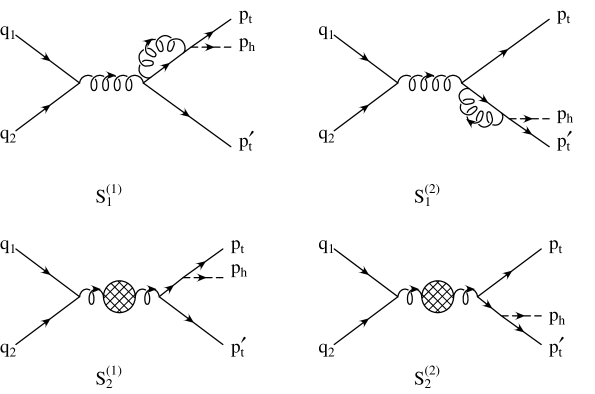
Figure 2: ${\cal O}(\alpha_{s})$ virtual corrections: self-energy diagrams $S_{1}^{(1,2)}$ and $S_{2}^{(1,2)}$.

3 Virtual Corrections

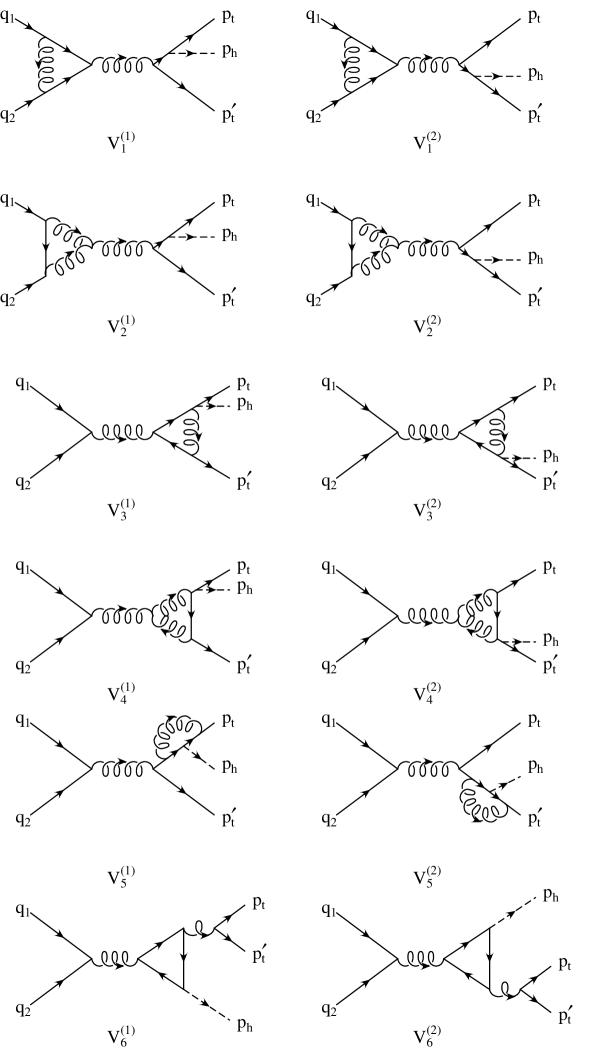
Figure 3: ${\cal O}(\alpha_{s})$ virtual corrections: vertex diagrams $V_{1}^{(1,2)}$-$V_{6}^{(1,2)}$.

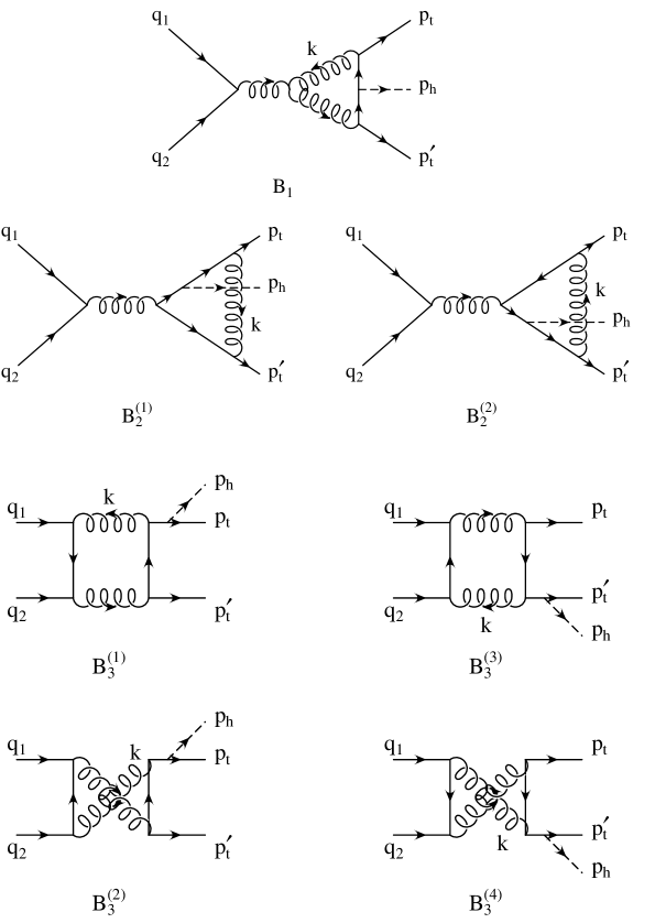
Figure 4: ${\cal O}(\alpha_{s})$ virtual corrections: box diagrams $B_{1}$, $B_{2}^{(1,2)}$ and $B_{3}^{(1-4)}$.

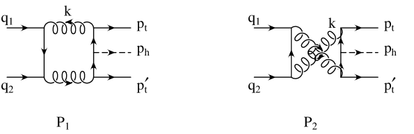
Figure 5: ${\cal O}(\alpha_{s})$ virtual corrections: pentagon diagrams $P_{1}$ and $P_{2}$.

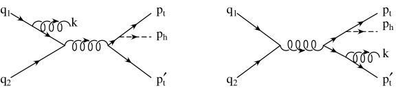
Figure 6: ${\cal O}(\alpha_{s})$ real corrections: examples of initial and final state real gluon emission.

The ${\cal O}(\alpha_{s})$ virtual corrections to the tree-level $q{\overline{q}}\rightarrow t{\overline{t}}h$ process consist of self-energy, vertex, box, and pentagon diagrams which are shown in Figs. 2-5. We assign incoming and outgoing momenta according to the following notation,

$$q(q_{1})+{\overline{q}}(q_{2})\rightarrow t(p_{t})+{\overline{t}}(p_{t}^{\prime})+h(p_{h})\,\,\,,$$ (9)

where the momentum flow is illustrated in Figs. 2-5. If we denote by ${\cal A}_{D_{i}}$ the amplitude associated with each virtual diagram $D_{i}$, the ${\cal O}(\alpha_{s}^{3})$ virtual amplitude squared can then be written as:

$$\overline{\sum}|{\cal A}_{virt}|^{2}=\sum_{i}\overline{\sum}\left({\cal A}_{\scriptscriptstyle LO}^{d}{\cal A}_{D_{i}}^{*}+{\cal A}_{\scriptscriptstyle LO}^{d*}{\cal A}_{D_{i}}\right)=\sum_{i}\overline{\sum}2\,{\cal R}e\left({\cal A}_{\scriptscriptstyle LO}^{d}{\cal A}_{D_{i}}^{*}\right)\,\,\,,$$ (10)

where the index $i$ runs over the set of all virtual diagrams, and ${\cal A}_{\scriptscriptstyle LO}^{d}$ denotes the tree-level amplitude for $q\bar{q}\rightarrow t\bar{t}h$ calculated in $d\!=\!4-2\epsilon$ dimensions. The lowest order amplitude ${\cal A}_{\scriptscriptstyle LO}^{d}$ must be computed to ${\cal O}(\epsilon^{2})$ in order to properly account for both the singular and finite contributions generated by the interference of ${\cal A}_{\scriptscriptstyle LO}^{d}$ with the single and double poles present in the virtual amplitudes ${\cal A}_{D_{i}}$. In what follows, we denote by ${\cal A}_{\scriptscriptstyle LO}$ the lowest order amplitude to ${\cal O}(\epsilon^{0})$, i.e. calculated in $d\!=\!4$ dimensions. Also, in the following sections, the contribution of a given diagram or set of diagrams to $\hat{\sigma}_{virt}^{q\bar{q}}$ is always to be understood as the contribution of the corresponding term in the sum in Eq. (10).

The calculation of the virtual diagrams has been performed using dimensional regularization, always in $d\!=\!4-2\epsilon$ dimensions. The diagrams have been evaluated using FORM [22] and Maple, and all tensor integrals have been reduced to linear combinations of a fundamental set of scalar one-loop integrals using standard techniques [23]. The scalar integrals which give rise to either ultraviolet (UV) or infrared (IR) singularities have been computed analytically, while finite scalar integrals have been evaluated using standard packages [24].

Self-energy and vertex diagrams contain both IR and UV divergences. The UV divergences are renormalized by introducing a suitable set of counterterms. Since the cross section is a renormalization group invariant, we only need to renormalize the wave function of the external fields, the top-quark mass, and the coupling constants. We discuss the renormalization of the UV singularities of the virtual cross section in Sec. 3.1.

Box and pentagon diagrams are ultraviolet finite, but have infrared singularities. The IR poles in the ${\cal O}(\alpha_{s})$ virtual corrections are eventually canceled by analogous singularities in the ${\cal O}(\alpha_{s})$ real corrections to the tree-level cross section. We discuss the structure of the IR singularities of the virtual cross section in Sec. 3.2. The structure of the IR singularities of the real cross section will be the subject of Secs. 4.1 and 4.2.

The calculation of many of the box scalar integrals and in particular of the pentagon scalar integrals are extremely laborious, due to the large number of massive particles present in the final state and in the loop. We have evaluated the necessary pentagon scalar integrals (one for diagram $P_{1}$ and one for diagram $P_{2}$), using the method of Ref. [11], which allows the reduction of a scalar five-point function to a sum of five scalar four-point functions, plus terms of $O(\epsilon)$ which can be neglected. Since this is a crucial ingredient of this calculation, we will explain in detail in Appendix A how the method of Ref. [11] has been applied to our case. The IR-divergent box scalar integrals are also collected in Appendix B.

3.1 UV singularities and counterterms

The UV singularities of the ${\cal O}(\alpha_{s}^{3})$ total cross section originate from self-energy and vertex virtual corrections. These singularities are renormalized by introducing counterterms for the wave function of the external fields ($\delta Z_{2}^{(q)}$, $\delta Z_{2}^{(t)}$), the top-quark mass ($\delta m_{t}$), and the coupling constants ($\delta g_{t}$, $\delta Z_{\alpha_{s}}$). If we denote by $\Delta_{UV}(S_{i}^{(1,2)})$ and $\Delta_{UV}(V_{i}^{(1,2)})$ the UV-divergent contribution of each self-energy ($S_{i}^{(1,2)}$) or vertex diagram ($V_{i}^{(1,2)}$) to the virtual amplitude squared (see Eq. (10)), we can write the UV-singular part of the total virtual amplitude squared as:

$$\overline{\sum}|{\cal A}_{virt}^{\scriptscriptstyle UV}|^{2} = \overline{\sum}|{\cal A}_{\scriptscriptstyle LO}|^{2}\,\left\{\sum_{i=1}^{2}\Delta_{UV}(S_{i}^{(1)}+S_{i}^{(2)})+\,\sum_{i=1}^{6}\Delta_{UV}(V_{i}^{(1)}+V_{i}^{(2)})\right.$$

$$+ \left.2\,\left[\,\left(\delta Z_{2}^{(q)}\right)_{UV}+\left(\delta Z_{2}^{(t)}\right)_{UV}+\frac{\delta m_{t}}{m_{t}}+\delta Z_{\alpha_{s}}\right]\right\}\,\,\,.$$

As described earlier, we denote by $|{\cal A}_{\scriptscriptstyle LO}|^{2}$ the matrix element squared of the tree-level amplitude for $q\bar{q}\rightarrow t\bar{t}h$, computed in $d=4$ dimensions. We also notice that, in writing Eq. (3.1), we have included in the top-quark self-energy the top-mass counterterm, and we have used the fact that the Yukawa-coupling counterterm coincides with the top-mass counterterm.

The UV-divergent contributions due to the individual diagrams are explicitly given by:

$$\Delta_{UV}\left(S_{1}^{(1)}+S_{1}^{(2)}\right) = \frac{\alpha_{s}}{2\pi}{\cal N}_{t}\left(\frac{N}{2}-\frac{1}{2N}\right)\biggl{(}-{1\over\epsilon_{\scriptscriptstyle UV}}\biggr{)}\,\,\,,$$

$$\Delta_{UV}\left(S_{2}^{(1)}+S_{2}^{(2)}\right) = \frac{\alpha_{s}}{2\pi}\biggl{[}{\cal N}_{s}\left(\frac{5}{3}N-\frac{2}{3}n_{lf}\right)-{\cal N}_{t}\frac{2}{3}\biggr{]}\biggl{(}{1\over\epsilon_{\scriptscriptstyle UV}}\biggr{)}\,\,\,,$$

$$\Delta_{UV}\left(V_{1}^{(1)}+V_{1}^{(2)}\right) = \frac{\alpha_{s}}{2\pi}{\cal N}_{s}\left(-{1\over 2N}\right)\biggl{(}{1\over\epsilon_{\scriptscriptstyle UV}}\biggr{)}\,\,\,,$$

$$\Delta_{UV}\left(V_{2}^{(1)}+V_{2}^{(2)}\right) = \frac{\alpha_{s}}{2\pi}{\cal N}_{s}\left(\frac{N}{2}\right)\biggl{(}{3\over\epsilon_{\scriptscriptstyle UV}}\biggr{)}\,\,\,,$$ (12)

$$\Delta_{UV}\left(V_{3}^{(1)}+V_{3}^{(2)}\right) = \frac{\alpha_{s}}{2\pi}{\cal N}_{t}\left(-{1\over 2N}\right)\biggl{(}{1\over\epsilon_{\scriptscriptstyle UV}}\biggr{)}\,\,\,,$$

$$\Delta_{UV}\left(V_{4}^{(1)}+V_{4}^{(2)}\right) = \frac{\alpha_{s}}{2\pi}{\cal N}_{t}\left(\frac{N}{2}\right)\biggl{(}{3\over\epsilon_{\scriptscriptstyle UV}}\biggr{)}\,\,\,,$$

$$\Delta_{UV}\left(V_{5}^{(1)}+V_{5}^{(2)}\right) = \frac{\alpha_{s}}{2\pi}{\cal N}_{t}\left(\frac{N}{2}-\frac{1}{2N}\right)\biggl{(}{4\over\epsilon_{\scriptscriptstyle UV}}\biggr{)}\,\,\,,$$

$$\Delta_{UV}\left(V_{6}^{(1)}+V_{6}^{(2)}\right) = 0\,\,\,,$$

where ${\cal N}_{s}$ and ${\cal N}_{t}$ are standard normalization factors defined as:

$${\cal N}_{s}=\biggl{(}{4\pi\mu^{2}\over s}\biggr{)}^{\epsilon}\Gamma(1+\epsilon)\,\,\,\,,\,\,\,\,{\cal N}_{t}=\biggl{(}{4\pi\mu^{2}\over m_{t}^{2}}\biggr{)}^{\epsilon}\Gamma(1+\epsilon)\,\,\,\,.$$ (13)

Moreover we define the needed counterterms according to the following convention. For the external fields, we fix the wave-function renormalization constants of the external fields ($Z_{2}^{(i)}=1+\delta Z_{2}^{(i)}$, $i\!=\!q,t$) using on-shell subtraction, i.e.:

$$\left(\delta Z_{2}^{(q)}\right)_{UV} = -\biggl{(}{\alpha_{s}\over 4\pi}\biggr{)}{\cal N}_{s}\biggl{(}{N\over 2}-{1\over 2N}\biggr{)}\biggl{(}{1\over\epsilon_{\scriptscriptstyle UV}}\biggr{)}\,\,\,,$$ (14)

$$\left(\delta Z_{2}^{(t)}\right)_{UV} = -\biggl{(}{\alpha_{s}\over 4\pi}\biggr{)}{\cal N}_{t}\biggl{(}{N\over 2}-{1\over 2N}\biggr{)}\biggl{(}{1\over\epsilon_{\scriptscriptstyle UV}}+4\biggr{)}\,\,\,.$$

We notice that both $\delta Z_{2}^{(q)}$ and $\delta Z_{2}^{(t)}$, as well as some of the vertex corrections ($V_{1}^{(1,2)}$ and $V_{2}^{(1,2)}$), have also IR singularities. In this section we limit the discussion to the UV singularities only, while the IR structure of these terms will be given explicitly in Sec. 3.2.

We define the subtraction condition for the top-quark mass $m_{t}$ in such a way that $m_{t}$ is the pole mass, in which case the top-mass counterterm is given by:

$${\delta m_{t}\over m_{t}}=-\biggl{(}{\alpha_{s}\over 4\pi}\biggr{)}{\cal N}_{t}\biggl{(}{N\over 2}-{1\over 2N}\biggr{)}\biggl{(}{3\over\epsilon_{\scriptscriptstyle UV}}+4\biggr{)}\,\,\,.$$ (15)

This counterterm has to be used twice: to renormalize the top-quark mass, in diagrams $S_{1}^{(1)}$ and $S_{1}^{(2)}$, and to renormalize the top-quark Yukawa coupling. As we already noted, $\Delta_{UV}(S_{1}^{(1)}+S_{1}^{(2)})$ in Eq. (3.1) already includes the top-mass counterterm.

Finally, for the renormalization of $\alpha_{s}$ we use the $\overline{MS}$ scheme, modified to decouple the top quark [25]. The first $n_{lf}$ light flavors are subtracted using the $\overline{MS}$ scheme, while the divergences associated with the top-quark loop are subtracted at zero momentum:

$$\delta Z_{\alpha_{s}}=\biggl{(}{\alpha_{s}\over 4\pi}\biggr{)}({4\pi})^{\epsilon}\Gamma(1+\epsilon)\biggl{[}\biggl{(}\frac{2}{3}n_{lf}-{11\over 3}N\biggr{)}{1\over\epsilon_{\scriptscriptstyle UV}}+\frac{2}{3}\biggl{(}{1\over\epsilon_{\scriptscriptstyle UV}}+\ln\biggl{(}\frac{\mu^{2}}{m_{t}^{2}}\biggr{)}\biggr{)}\biggr{]}\,\,\,,$$ (16)

such that, in this scheme, the renormalized strong coupling constant $\alpha_{s}$ evolves with $n_{lf}=5$ light flavors.

It is easy to verify that the sum of all the UV-singular contributions as given in Eq. (3.1) is finite. We also notice that the left over renormalization scale dependence, due to the mismatch between the renormalization scale dependence of $\Delta_{UV}(S_{2})$ and $\delta(Z_{\alpha_{s}})$, is given by:

$$\overline{\sum}|{\cal A}_{\scriptscriptstyle LO}|^{2}{\alpha_{s}(\mu)\over 2\pi}\left(-\frac{2}{3}n_{lf}+\frac{11}{3}N\right)\ln\left(\frac{\mu^{2}}{s}\right)\,\,\,,$$ (17)

and corresponds exactly to the first term of Eq. (2), as predicted by renormalization group arguments.

3.2 IR singularities

This section describes the structure of the IR singularities originating from the ${\cal O}(\alpha_{s})$ virtual corrections. The virtual IR singularities come from the following set of diagrams: vertex diagrams $V_{1}^{(1,2)}$ and $V_{2}^{(1,2)}$, box diagrams $B_{2}^{(1,2)}$, box diagrams $B_{3}^{(1-4)}$, pentagon diagrams $P_{1}$ and $P_{2}$, and from the wave function renormalization of the external fields, $\delta Z_{2}^{(q)}$ and $\delta Z_{2}^{(t)}$. The IR-singular part of the total virtual amplitude squared is then of the form:

$$\overline{\sum}|{\cal A}_{virt}^{\scriptscriptstyle IR}|^{2} = \overline{\sum}|{\cal A}_{\scriptscriptstyle LO}|^{2}\left\{\Delta_{IR}\left(V_{1}^{(1)}+V_{1}^{(2)}\right)+\Delta_{IR}\left(V_{2}^{(1)}+V_{2}^{(2)}\right)+\left(\delta Z_{2}^{(q)}\right)_{IR}+\left(\delta Z_{2}^{(q)}\right)_{IR}\right.$$ (18)

$$\!\!\!\!\!\!\!\!\!\!\!\!\left.+\,\Delta_{IR}\left(B_{2}^{(1)}+B_{2}^{(2)}\right)+\Delta_{IR}\left(B_{3}^{(1)}+B_{3}^{(3)}+P_{1}\right)+\Delta_{IR}\left(B_{3}^{(2)}+B_{3}^{(4)}+P_{1}\right)\right\}\,\,\,,$$

where, as before, $|{\cal A}_{\scriptscriptstyle LO}|^{2}$ denotes the matrix element squared of the tree-level amplitude for $q\bar{q}\rightarrow t\bar{t}h$, in $d\!=\!4$ dimensions. The IR-divergent contributions of the various diagrams to the virtual amplitude squared are given in the following:

$$\Delta_{IR}\left(V_{1}^{(1)}+V_{1}^{(2)}\right) = \left(\frac{\alpha_{s}}{2\pi}\right){\cal N}_{s}\left(-\frac{1}{2N}\right)\left(-\frac{2}{\epsilon_{\scriptscriptstyle IR}^{2}}-\frac{4}{\epsilon_{\scriptscriptstyle IR}}\right)\,\,\,,$$

$$\Delta_{IR}\left(V_{2}^{(1)}+V_{2}^{(2)}\right) = \left(\frac{\alpha_{s}}{2\pi}\right){\cal N}_{s}\left(\frac{N}{2}\right)\left(-\frac{4}{\epsilon_{\scriptscriptstyle IR}}\right)\,\,\,,$$

$$\left(\delta Z_{2}^{(q)}\right)_{IR} = \left(\frac{\alpha_{s}}{2\pi}\right){\cal N}_{s}\left(\frac{N}{2}-\frac{1}{2N}\right)\left(\frac{1}{\epsilon_{\scriptscriptstyle IR}}\right)\,\,\,,$$ (19)

$$\left(\delta Z_{2}^{(t)}\right)_{IR} = \left(\frac{\alpha_{s}}{2\pi}\right){\cal N}_{t}\left(\frac{N}{2}-\frac{1}{2N}\right)\left(-\frac{2}{\epsilon_{\scriptscriptstyle IR}}\right)\,\,\,,$$

$$\Delta_{IR}\left(B_{2}^{(1)}+B_{2}^{(2)}\right) = \left(\frac{\alpha_{s}}{2\pi}\right){\cal N}_{t}\left(-\frac{1}{N}\right)\left(\frac{1}{\epsilon_{\scriptscriptstyle IR}}\frac{s_{t\bar{t}}}{(2m_{t}^{2}+s_{t\bar{t}})\beta_{t\bar{t}}}\Lambda_{t\bar{t}}\right)\,\,\,,$$

$$\Delta_{IR}\left(B_{3}^{(1)}+B_{3}^{(3)}+P_{1}\right) = \left(\frac{\alpha_{s}}{2\pi}\right){\cal N}_{t}\left(\frac{N}{2}-\frac{1}{N}\right)\left[-\frac{2}{\epsilon_{\scriptscriptstyle IR}^{2}}+\frac{2}{\epsilon_{\scriptscriptstyle IR}}\left(\ln\left(\frac{s_{qt}}{m_{t}^{2}}\right)+\ln\left(\frac{s_{\bar{q}\bar{t}}}{m_{t}^{2}}\right)\right)\right]\,\,\,,$$

$$\Delta_{IR}\left(B_{3}^{(2)}+B_{3}^{(4)}+P_{2}\right) = \left(\frac{\alpha_{s}}{2\pi}\right){\cal N}_{t}\left(-\frac{1}{N}\right)\left[\frac{2}{\epsilon^{2}_{\scriptscriptstyle IR}}-\frac{2}{\epsilon_{\scriptscriptstyle IR}}\left(\ln\left(\frac{s_{q\bar{t}}}{m_{t}^{2}}\right)+\ln\left(\frac{s_{\bar{q}t}}{m_{t}^{2}}\right)\right)\right]\,\,\,,$$

where ${\cal N}_{s}$ and ${\cal N}_{t}$ are given in Eq. (13). Moreover, we have introduced the following kinematic invariants:

$$s\!=s_{q\bar{q}}=\!2q_{1}\cdot q_{2}\,\,\,,\,\,\,s_{t\bar{t}}\!=\!2p_{t}\cdot p_{t}^{\prime}\,\,\,,\,\,\,s_{qt}\!=\!2q_{1}\cdot p_{t}\,\,\,,\,\,\,s_{q\bar{t}}\!=\!2q_{1}\cdot p_{t}^{\prime}\,\,\,,\,\,\,s_{\bar{q}t}\!=\!2q_{2}\cdot p_{t}\,\,\,,\,\,\,s_{\bar{q}\bar{t}}\!=\!2q_{2}\cdot p_{t}^{\prime}\,\,\,,\,\,\,$$ (20)

and we have defined

$$\beta_{t\bar{t}} = \sqrt{1-{4m_{t}^{2}\over(p_{t}+p_{t}^{\prime})^{2}}}\,\,\,,$$ (21)

$$\Lambda_{t\bar{t}} = \ln\biggl{(}{1+\beta_{t\bar{t}}\over 1-\beta_{t\bar{t}}}\biggr{)}\,\,\,.$$

Substituting the explicit expression for the IR-divergent contributions given in Eq. (3.2) into Eq. (18) yields:

$$\overline{\sum}|{\cal A}_{virt}^{\scriptscriptstyle IR}|^{2}=\left(\frac{\alpha_{s}}{2\pi}\right){\cal N}_{t}\,\overline{\sum}|{\cal A}_{\scriptscriptstyle LO}|^{2}\left\{\frac{X_{-2}^{virt}}{\epsilon_{\scriptscriptstyle IR}^{2}}+\frac{X_{-1}^{virt}}{\epsilon_{\scriptscriptstyle IR}}+\delta_{virt}^{\scriptscriptstyle IR}\right\}\,\,\,,$$ (22)

where

$$X_{-2}^{virt} = -\left(N-\frac{1}{N}\right)\,\,\,,$$ (23)

$$X_{-1}^{virt} = N\,\left[-\frac{5}{2}+\ln\left(\frac{s_{qt}}{m_{t}^{2}}\right)+\ln\left(\frac{s_{\bar{q}\bar{t}}}{m_{t}^{2}}\right)\right]$$

$$+ \frac{1}{N}\,\left[-\ln\left(\frac{s}{m_{t}^{2}}\right)+\frac{5}{2}-\frac{s_{t\bar{t}}}{(2m_{t}^{2}+s_{t\bar{t}})\beta_{t\bar{t}}}\Lambda_{t\bar{t}}-2\ln\left(\frac{s_{qt}s_{\bar{q}\bar{t}}}{s_{q\bar{t}}s_{\bar{q}t}}\right)\right]\,\,\,,$$

while $\delta_{virt}^{IR}$ is a finite term that derives from having factored out a common factor ${\cal N}_{t}$, and is given by:

$$\delta_{virt}^{\scriptscriptstyle IR}=\left(N-\frac{1}{N}\right)\left[\frac{3}{2}\ln\left(\frac{s}{m_{t}^{2}}\right)\right]+\frac{1}{N}\left[\frac{1}{2}\ln^{2}\left(\frac{s}{m_{t}^{2}}\right)\right]\,\,\,.$$ (24)

In Secs. 4.1.1 and 4.2.3 we will show how the IR singularities of the real cross section exactly cancel the IR poles of the virtual cross section (see Eqs. (33)-(34) and Eqs. (76)-(77)), as predicted by the Bloch-Nordsieck [26] and Kinoshita-Lee-Nauenberg [27, 28] theorems.

4 Real Corrections

The ${\cal O}(\alpha_{s})$ corrections to $q\bar{q}\rightarrow t\bar{t}h$ due to real gluon emission (see Fig. 6) give origin to IR singularities which cancel exactly the analogous singularities present in the ${\cal O}(\alpha_{s})$ virtual corrections (see Sec. 3.2). These singularities can be either of soft or collinear nature and can be conveniently isolated by slicing the $q\bar{q}\rightarrow t\bar{t}h+g$ phase space into different regions defined by suitable cutoffs, a method which goes under the general name of Phase Space Slicing (PSS). The dependence on the arbitrary cutoff(s) introduced in the process is not physical, and, in fact, cancels at the level of the total real gluon emission hadronic cross section, i.e. in $\sigma_{real}$, the real part of $\sigma_{\scriptscriptstyle NLO}$ . This constitutes an important check of the calculation.

We have calculated the cross section for the process

$$q(q_{1})+{\overline{q}}(q_{2})\rightarrow t(p_{t})+{\overline{t}}(p_{t}^{\prime})+h(p_{h})+g(k)$$ (25)

using two different implementations of the PSS method which we call the two-cutoff and one-cutoff method respectively, depending on the number of cutoffs introduced. The two-cutoff implementation of the PSS method has been originally developed to study QCD corrections to dihadron production [12] and has since then been applied to a variety of processes. A nice review has recently appeared [13] to which we refer for more extensive references and details. The one-cutoff PSS method has been developed for massless quarks in Ref. [14, 15] and extended to the case of massive quarks in Ref. [16].

In the next two sections we explain in detail how we have applied the PSS method to our case, using the two-cutoff implementation in Sec. 4.1 and the one-cutoff implementation in Sec. 4.2. The results for $\sigma_{real}$ obtained using PSS with one or two cutoffs agree within the statistical errors. In spite of the fact that both methods are realizations of the general idea of phase space slicing, they have very different characteristics and finding agreement between the two represents an important check of our calculation.

4.1 Phase Space Slicing method with two cutoffs

The general implementation of the PSS method using two cutoffs proceeds in two steps. First, by introducing an arbitrary small soft cutoff $\delta_{s}$ we separate the overall integration of the $q\bar{q}\rightarrow t\bar{t}h+g$ phase space into two regions, according to whether the energy of the gluon is soft, i.e. $E_{g}\leq\delta_{s}\sqrt{s}/2$, or hard, i.e. $E_{g}>\delta_{s}\sqrt{s}/2$. The partonic real cross section of Eq. (5) can then be written as:

$$\hat{\sigma}^{q\bar{q}}_{real}=\hat{\sigma}_{soft}+\hat{\sigma}_{hard}\,\,\,,$$ (26)

where $\hat{\sigma}_{soft}$ is obtained by integrating over the soft region of the gluon phase space, and contains all the IR soft divergences of $\hat{\sigma}_{real}^{q\bar{q}}$. To isolate the remaining collinear divergences from $\hat{\sigma}_{hard}$, we further split the integration over the hard gluon phase space according to whether the gluon is ($\hat{\sigma}_{hard/coll}$) or is not ($\hat{\sigma}_{hard/non-coll}$) emitted within an angle $\theta$ from the initial-state massless quarks such that $(1-\cos\theta)<\delta_{c}$, for an arbitrary small collinear cutoff $\delta_{c}$:

$$\hat{\sigma}_{hard}=\hat{\sigma}_{hard/coll}+\hat{\sigma}_{hard/non-coll}\,\,\,.$$ (27)

The hard non-collinear part of the real cross section, $\hat{\sigma}_{hard/non-coll}$, is finite and can be computed numerically, using standard Monte-Carlo techniques. In the soft and collinear regions, the integration over the phase space of the emitted gluon can be performed analytically, thus allowing us to isolate the IR collinear divergences of $\hat{\sigma}_{real}^{q\bar{q}}$. More details on the calculation of $\hat{\sigma}_{soft}$ and $\hat{\sigma}_{hard}$ are given in Sec. 4.1.1 and Sec. 4.1.2, respectively. The cross sections describing soft, collinear and IR-finite gluon radiation depend on the two arbitrary parameters, $\delta_{s}$ and $\delta_{c}$. However, in the real hadronic cross section $\sigma_{real}$, after mass factorization, the dependence on these arbitrary cutoffs cancels, as will be explicitly shown in Sec. 5.

4.1.1 Soft gluon emission

The soft region of the $q\bar{q}\rightarrow t\bar{t}h+g$ phase space is defined by requiring that the energy of the gluon satisfies:

$$E_{g}<\delta_{s}{\sqrt{s}\over 2}\,\,\,,$$ (28)

for an arbitrary small value of the soft cutoff $\delta_{s}$. In the limit when the energy of the gluon becomes small, i.e. in the soft limit, the matrix element squared for the real gluon emission, $\overline{\sum}|{\cal A}_{real}|^{2}$, assumes a very simple form, i.e. it factorizes into the Born matrix element squared times an eikonal factor $\Phi_{eik}$:

$$\overline{\sum}|{\cal A}_{real}(q\bar{q}\rightarrow t\bar{t}h+g)|^{2}\stackrel{{\scriptstyle soft}}{{\longrightarrow}}(4\pi\alpha_{s})\overline{\sum}|{\cal A}_{\scriptscriptstyle LO}|^{2}\,\Phi_{eik}\,\,\,,$$ (29)

where the eikonal factor is given by:

$$\Phi_{eik} = \frac{N}{2}\left[-\frac{m_{t}^{2}}{(p_{t}\!\cdot\!k)^{2}}-\frac{m_{t}^{2}}{(p_{t}^{\prime}\!\cdot\!k)^{2}}+\frac{s_{qt}}{(q_{1}\!\cdot\!k)(p_{t}\!\cdot\!k)}+\frac{s_{\bar{q}\bar{t}}}{(q_{2}\!\cdot\!k)(p_{t}^{\prime}\!\cdot\!k)}\right]$$

$$+\frac{1}{2N}\left[\frac{m_{t}^{2}}{(p_{t}\!\cdot\!k)^{2}}+\frac{m_{t}^{2}}{(p_{t}^{\prime}\!\cdot\!k)^{2}}-\frac{s}{(q_{1}\!\cdot\!k)(q_{2}\!\cdot\!k)}-\frac{s_{t\bar{t}}}{(p_{t}\!\cdot\!k)(p_{t}^{\prime}\!\cdot\!k)}\right.$$

$$\left.+2\left(-\frac{s_{qt}}{(q_{1}\!\cdot\!k)(p_{t}\!\cdot\!k)}+\frac{s_{q\bar{t}}}{(q_{1}\!\cdot\!k)(p_{t}^{\prime}\!\cdot\!k)}+\frac{s_{\bar{q}t}}{(q_{2}\!\cdot\!k)(p_{t}\!\cdot\!k)}-\frac{s_{\bar{q}\bar{t}}}{(q_{2}\!\cdot\!k)(p_{t}^{\prime}\!\cdot\!k)}\right)\right]\,\,\,.$$

Moreover, in the soft region the $q\bar{q}\rightarrow t\bar{t}h+g$ phase space also factorizes as:

$$d(PS_{4})(q\bar{q}\rightarrow t\bar{t}h+g) \stackrel{{\scriptstyle soft}}{{\longrightarrow}} d(PS_{3})(q\bar{q}\rightarrow t\bar{t}h)d(PS_{g})_{soft}$$

$$= d(PS_{3})(q\bar{q}\rightarrow t\bar{t}h)\frac{d^{(d-1)}k}{(2\pi)^{(d-1)}2E_{g}}\theta(\delta_{s}{\sqrt{s}\over 2}-E_{g})\,\,\,,$$

where $d(PS_{g})_{soft}$ denotes the integration over the phase space of the soft gluon. The parton level soft cross section can then be written as:

$$\hat{\sigma}_{soft}=(4\pi\alpha_{s})\,\mu^{2\epsilon}\,\int d(PS_{3})\overline{\sum}|{\cal A}_{\scriptscriptstyle LO}|^{2}\int d(PS_{g})_{soft}\Phi_{eik}\,\,\,.$$ (32)

Since the contribution of the soft gluon is now completely factorized, we can perform the integration over $d(PS_{g})_{soft}$ in Eq. (32) analytically, and extract the soft poles that will have to cancel $X_{-2}^{virt}$ and $X_{-1}^{virt}$ of Eq. (23). The integration over the gluon phase space in Eq. (32) can be performed using standard techniques and we refer to Refs. [13, 29] for more details. For sake of completeness, in Appendix C we give explicit results for the soft integrals used in our calculation.

Finally, the soft gluon contribution to $\hat{\sigma}_{real}^{q\bar{q}}$ can be written as follows:

$$\hat{\sigma}_{soft}=\frac{\alpha_{s}}{2\pi}{\cal N}_{t}\int d(PS_{3})\overline{\sum}|{\cal A}_{\scriptscriptstyle LO}|^{2}\left\{\frac{X_{-2}^{s}}{\epsilon^{2}}+\frac{X_{-1}^{s}}{\epsilon}+NC_{1}^{s}+\frac{C_{2}^{s}}{N}\right\}\,\,\,,$$ (33)

where

$$X_{-2}^{s} = -X_{-2}^{virt}\,\,\,,$$ (34)

$$X_{-1}^{s} = -X_{-1}^{virt}-\left(N-\frac{1}{N}\right)\,\left[\frac{3}{2}+2\ln\left(\delta_{s}\right)\right]\,\,\,,$$

$$C_{1}^{s} = \frac{3}{2}\ln\left(\frac{s}{\mu^{2}}\right)+2\ln^{2}(\delta_{s})-2\ln(\delta_{s})\left[1+\ln\left({m_{t}^{2}\mu^{2}\over s_{qt}s_{\bar{q}\bar{t}}}\right)\right]$$

$$+{1\over 2}\ln^{2}\biggl{(}{s\over m_{t}^{2}}\biggr{)}-{\pi^{2}\over 3}-\ln\biggl{(}{s\over m_{t}^{2}}\biggr{)}\biggl{[}{5\over 2}+\ln\biggl{(}{sm_{t}^{2}\over s_{qt}s_{\bar{q}\bar{t}}}\biggr{)}\biggr{]}$$

$$+{\Lambda_{t\bar{t}}\over\beta_{t\bar{t}}}+{1\over 2}\biggl{[}F_{qt}+F_{\bar{q}\bar{t}}\biggr{]}+\left[\frac{3}{2}+2\ln\left(\delta_{s}\right)\right]\,\ln\left(\frac{\mu^{2}}{m_{t}^{2}}\right)\,\,\,,$$

$$C_{2}^{s} = -{3\over 2}\ln\biggl{(}{s\over\mu^{2}}\biggr{)}-2\ln^{2}(\delta_{s})-2\ln(\delta_{s})\biggl{[}-1+\frac{s_{t\bar{t}}}{(2m_{t}^{2}+s_{t\bar{t}})\beta_{t\bar{t}}}\Lambda_{t\bar{t}}$$

$$+\ln\biggl{(}{s\over\mu^{2}}\biggr{)}+2\ln\biggl{(}{s_{qt}s_{\bar{q}\bar{t}}\over s_{q\bar{t}}s_{\bar{q}t}}\biggr{)}\biggr{]}$$

$$-{1\over 2}\ln^{2}\biggl{(}{s\over m_{t}^{2}}\biggr{)}+{\pi^{2}\over 3}-\ln\biggl{(}{s\over m_{t}^{2}}\biggr{)}\biggl{[}-{5\over 2}+\frac{s_{t\bar{t}}}{(2m_{t}^{2}+s_{t\bar{t}})\beta_{t\bar{t}}}\Lambda_{t\bar{t}}$$

$$+2\ln\biggl{(}{s_{qt}s_{\bar{q}\bar{t}}\over s_{q\bar{t}}s_{\bar{q}t}}\biggr{)}\biggr{]}-{\Lambda_{t\bar{t}}\over\beta_{t\bar{t}}}$$

$$+\frac{2s_{t\bar{t}}}{(2m_{t}^{2}+s_{t\bar{t}})\beta_{t\bar{t}}}\biggl{[}\mbox{Li}_{2}\biggl{(}{2\beta_{t\bar{t}}\over 1+\beta_{t\bar{t}}}\biggr{)}+{1\over 4}\ln^{2}\biggl{(}{1+\beta_{t\bar{t}}\over 1-\beta_{t\bar{t}}}\biggr{)}\biggr{]}$$

$$-F_{qt}+F_{q\bar{t}}+F_{\bar{q}t}v-F_{\bar{q}\bar{t}}-\left[\frac{3}{2}+2\ln\left(\delta_{s}\right)\right]\,\ln\left(\frac{\mu^{2}}{m_{t}^{2}}\right)\,\,\,,$$

while ${\cal N}_{t}$ is defined in Eq. (13), and $\mbox{Li}_{2}$ denotes the dilogarithm as described in Ref. [30]. $\beta_{t\bar{t}}$ and $\Lambda_{t\bar{t}}$ are defined in Eq. (21), while, for any initial parton $i$ and final parton $f$, the function $F_{if}$ can be written as:

$$F_{if} = \ln^{2}\biggl{(}{1-\beta_{f}\over 1-\beta_{f}\cos\theta_{if}}\biggr{)}-{1\over 2}\ln^{2}\biggl{(}{1+\beta_{f}\over 1-\beta_{f}}\biggr{)}$$

$$+2\mbox{Li}_{2}\biggl{(}-{\beta_{f}(1-\cos\theta_{if})\over 1-\beta_{f}}\biggr{)}-2\mbox{Li}_{2}\biggl{(}-{\beta_{f}(1+\cos\theta_{if})\over 1-\beta_{f}\cos\theta_{if}}\biggr{)}\,\,\,,$$

where $\cos\theta_{if}$ is the angle between partons $i$ and $f$ in the center-of-mass frame of the initial state partons, and

$$\beta_{f}=\sqrt{1-\frac{m_{t}^{2}}{(p_{f}^{0})^{2}}}\,\,\,\,\,,\,\,\,\,\,1-\beta_{f}\cos{\theta_{if}}=\frac{s_{if}}{p_{f}^{0}\sqrt{s}}\,\,\,.$$ (36)

All the quantities in Eq. (4.1.1) can be expressed in terms of kinematic Al invariants, once we use $s_{if}\!=\!2p_{i}\!\cdot\!p_{f}$ together with:

$$p_{t}^{0}=\frac{s-{\bar{s}}_{{\bar{t}}h}+m_{t}^{2}}{2\sqrt{s}}\,\,\,\,\,\mbox{and}\,\,\,\,\,p_{\bar{t}}^{0}=\frac{s-{\bar{s}}_{th}+m_{t}^{2}}{2\sqrt{s}}\,\,\,,$$ (37)

where ${\bar{s}}_{fh}\!=\!(p_{f}+p_{h})^{2}$. As can be easily seen from Eqs. (23) and (34), the IR poles of the virtual corrections are exactly canceled by the corresponding singularities in the soft gluon contribution. The remaining IR poles in $\hat{\sigma}_{soft}$ will be canceled by the PDF counterterms as described in detail in Sec. 5.

4.1.2 Hard gluon emission

The hard region of the gluon phase space is defined by requiring that the energy of the emitted gluon is above a given threshold. As we discussed earlier this is expressed by the condition that

$$E_{g}>\delta_{s}{\sqrt{s}\over 2}\,\,\,,$$ (38)

for an arbitrary small soft cutoff $\delta_{s}$, which automatically assures that $\hat{\sigma}_{hard}$ does not contain soft singularities. However, a hard gluon can still give origin to singularities when it is emitted at a small angle, i.e. collinear, to a massless incoming or outgoing parton. In order to isolate these divergences and compute them analytically, we further divide the hard region of the $q\bar{q}\rightarrow t\bar{t}h+g$ phase space into a hard/collinear and a hard/non-collinear region, by introducing a second small collinear cutoff $\delta_{c}$. The hard/non-collinear region is defined by the condition that both

$$\frac{2q_{1}\!\cdot\!k}{E_{g}\sqrt{s}}>\delta_{c}\,\,\,\,\,\,\,\mbox{and}\,\,\,\,\,\,\,\frac{2q_{2}\!\cdot\!k}{E_{g}\sqrt{s}}>\delta_{c}$$ (39)

are verified. The contribution from the hard/non-collinear region, $\hat{\sigma}_{hard/non-coll}$, is finite and we compute it numerically by using standard Monte Carlo integration techniques.

In the hard/collinear region, one of the conditions in Eq. (39) is not satisfied and the hard gluon is emitted collinear to one of the incoming partons. In this region, the initial-state parton $i$ ($i\!=\!q,\bar{q}$) is considered to split into a hard parton $i^{\prime}$ and a collinear gluon $g$, $i\rightarrow i^{\prime}g$, with $p_{i^{\prime}}\!=\!zp_{i}$ and $k\!=\!(1-z)p_{i}$. The matrix element squared for $ij\rightarrow t\bar{t}h+g$ factorizes into the Born matrix element squared and the Altarelli-Parisi splitting function for $i\rightarrow i^{\prime}g$, i.e.:

$$\overline{\sum}|{\cal A}_{real}(ij\rightarrow t\bar{t}h+g)|^{2}\stackrel{{\scriptstyle collinear}}{{\longrightarrow}}(4\pi\alpha_{s})\sum_{i}\overline{\sum}|{\cal A}_{\scriptscriptstyle LO}(i^{\prime}j\rightarrow t\bar{t}h)|^{2}\frac{2P_{ii^{\prime}}(z)}{z\,s_{ig}}\,\,\,,$$ (40)

with $s_{ig}=2p_{i}\!\cdot\!k$. In our case:

$$P_{ii^{\prime}}(z)=P_{qq}(z)=C_{F}\left(\frac{1+z^{2}}{1-z}-\epsilon(1-z)\right)$$ (41)

is the unregulated Altarelli-Parisi splitting function for $q\!\rightarrow\!q+g$ at lowest order, including terms of ${\cal O}(\epsilon)$, and $C_{F}\!=\!(N^{2}-1)/2N$. Moreover, in the collinear limit, the $q\bar{q}\rightarrow t\bar{t}h+g$ phase space also factorizes as:

$$d(PS_{4})(ij\rightarrow t\bar{t}h+g) \stackrel{{\scriptstyle collinear}}{{\longrightarrow}} d(PS_{3})(i^{\prime}j\rightarrow t\bar{t}h)\frac{z\,d^{(d-1)}k}{(2\pi)^{(d-1)}2E_{g}}\theta\left(E_{g}-\delta_{s}{\sqrt{s}\over 2}\right)\times$$

$$\theta(\cos\theta_{ig}-(1-\delta_{c}))$$

$$\!\!\!\!\!\!\!\!\!\!\!\!\!\!\!\!\!\!\!\!\!\!\stackrel{{\scriptstyle d=4-2\epsilon}}{{=}}\frac{\Gamma(1-\epsilon)}{\Gamma(1-2\epsilon)}\frac{\left(4\pi\right)^{\epsilon}}{16\pi^{2}}\,z\,dz\,ds_{ig}\left[(1-z)s_{ig}\right]^{-\epsilon}\theta\left({(1-z)\over z}s^{\prime}{\delta_{c}\over 2}-s_{ig}\right)\;,$$

where the integration range for $s_{ig}$ in the collinear region is given in terms of the collinear cutoff, and we have defined $s^{\prime}\!=\!2p_{i^{\prime}}\cdot p_{j}$. The integral over the collinear gluon degrees of freedom can then be performed separately, and this allows us to explicitly extract the collinear singularities of $\hat{\sigma}_{hard}$. $\hat{\sigma}_{hard/coll}$ turns out to be of the form [13, 31]:

$$\hat{\sigma}_{hard/coll} = \left[\frac{\alpha_{s}}{2\pi}\frac{\Gamma(1-\epsilon)}{\Gamma(1-2\epsilon)}\left(\frac{4\pi\mu^{2}}{m_{t}^{2}}\right)^{\epsilon}\right]\left(-\frac{1}{\epsilon}\right)\delta_{c}^{-\epsilon}\times$$

$$\left\{\int_{0}^{1-\delta_{s}}dz\left[\frac{(1-z)^{2}}{2z}\frac{s^{\prime}}{m_{t}^{2}}\right]^{-\epsilon}P_{ii^{\prime}}(z)\,\hat{\sigma}_{\scriptscriptstyle LO}(i^{\prime}j\rightarrow t\bar{t}h)+(i\leftrightarrow j)\right\}\,\,\,.$$

The upper limit on the $z$ integration ensures the exclusion of the soft gluon region. As usual, these initial-state collinear divergences are absorbed into the parton distribution functions as will be described in detail in the Sec. 5.

4.2 Phase Space Slicing method with one cutoff

An alternative way of isolating both soft and collinear singularities is to divide the phase space of the final state partons into two regions according to whether all partons can be resolved (the hard region) or not (the infrared, or ir, region). In the case of $q\bar{q}\rightarrow t\bar{t}h+g$, the hard and ir regions are defined by whether the gluon is resolved or not. The emitted gluon is not resolved, and therefore considered ir, when

$$s_{ig}=2p_{i}\cdot k<s_{min}\,\,\,,\,\,\,\mbox{with}\,\,\,\,\,i=q,\bar{q},t,\bar{t}\,\,\,,$$ (44)

for an arbitrary small cutoff $s_{min}$. Similarly to Eq. (26), the partonic real cross section can be written as the sum of two terms:

$$\hat{\sigma}_{real}^{q\bar{q}}=\hat{\sigma}_{ir}+\hat{\sigma}_{hard}\,\,\,,$$ (45)

where $\hat{\sigma}_{ir}$ includes both soft and collinear singularities, while $\hat{\sigma}_{hard}$ is finite. Following the general idea of PSS, we calculate $\hat{\sigma}_{ir}$ analytically, while we evaluate $\hat{\sigma}_{hard}$ numerically, using standard Monte Carlo integration techniques. Both $\hat{\sigma}_{ir}$ and $\hat{\sigma}_{hard}$ depend on the cutoff $s_{min}$, but the hadronic real cross section, $\sigma_{real}$, is cutoff independent, after mass factorization, as will be shown in Sec. 5.

In order to calculate $\hat{\sigma}_{ir}$ we apply the formalism developed in Refs. [14, 15, 16] as follows.

• We consider the crossed process $h\rightarrow q\bar{q}t\bar{t}+g$ which is obtained from $q\bar{q}\rightarrow t\bar{t}h+g$ by crossing all the initial state colored partons to the final state, while crossing the Higgs boson to the initial state. For a systematic extraction of the IR singularities within the one-cutoff method, we organize the amplitude for $h\rightarrow q\bar{q}t\bar{t}+g$, ${\cal A}^{h\to q\bar{q}t\bar{t}g}$, in terms of colored ordered amplitudes [32]. Using the color decomposition:

  $$T^{a}_{c_{1}c_{2}}T^{a}_{c_{3}c_{4}}=\frac{1}{2}\left(\delta_{c_{1}c_{4}}\delta_{c_{3}c_{2}}-\frac{1}{N}\delta_{c_{1}c_{2}}\delta_{c_{3}c_{4}}\right)\,\,\,,$$ (46)

  we write ${\cal A}^{h\to q\bar{q}t\bar{t}g}$ as the sum of four color ordered amplitudes ${\cal A}_{1},\ldots,{\cal A}_{4}$ as follows:

  $${\cal A}^{h\to q\bar{q}t\bar{t}g} = ig_{s}\delta_{f_{q}f_{\bar{q}}}\delta_{f_{t}f_{\bar{t}}}\frac{1}{2}\left(\delta_{c_{t}c_{\bar{q}}}T^{a}_{c_{q}c_{\bar{t}}}{\cal A}_{1}(p_{t},p_{t}^{\prime},q_{1},q_{2},k)+T^{a}_{c_{t}c_{\bar{q}}}\delta_{c_{q}c_{\bar{t}}}{\cal A}_{2}(p_{t},p_{t}^{\prime},q_{1},q_{2},k)\right.$$ (47)

  $$- \left.\frac{1}{N}\delta_{c_{t}c_{\bar{t}}}T^{a}_{c_{q}c_{\bar{q}}}{\cal A}_{3}(p_{t},p_{t}^{\prime},q_{1},q_{2},k)-\frac{1}{N}T^{a}_{c_{t}c_{\bar{t}}}\delta_{c_{q}c_{\bar{q}}}{\cal A}_{4}(p_{t},p_{t}^{\prime},q_{1},q_{2},k)\right)\,\,\,,$$

  where $g_{s}\!=\!\sqrt{4\pi\alpha_{s}}$, while $(f_{q},f_{\bar{q}},f_{t},f_{\bar{t}})$ and $(c_{q},c_{\bar{q}},c_{t},c_{\bar{t}})$ denote the flavor and color indices of the various outgoing quarks. The amplitudes ${\cal A}_{i}(p_{t},p_{t}^{\prime},q_{1},q_{2},k)$ (for $i=1,2,3,4$) correspond to the four possible independent color structures that arise in the $h\rightarrow t\bar{t}q\bar{q}+g$ process, and each ${\cal A}_{i}$ contains terms describing the emission of the gluon from a different pair of external quarks. We give the explicit expressions for the ${\cal A}_{i}$ amplitudes in Appendix D. Due to this decomposition, the partonic cross section for $h\to q\bar{q}t\bar{t}+g$ can be written in a very compact form:

  $$\hat{\sigma}^{h\to q\bar{q}t\bar{t}g}=\int d(PS_{5})\overline{\sum}|{\cal A}^{h\to q\bar{q}t\bar{t}g}|^{2}\,\,\,,$$ (48)

  with

  $$\overline{\sum}|{\cal A}^{h\to q\bar{q}t\bar{t}g}|^{2} = \left({g_{s}^{2}N\over 2}\right)\left(\frac{N^{2}-1}{4}\right)\overline{\sum}\left\{|{\cal A}_{1}|^{2}+|{\cal A}_{2}|^{2}+\right.$$

  $$\left.\frac{1}{N^{2}}\left[-2|{\cal A}_{3}+{\cal A}_{4}|^{2}+|{\cal A}_{3}|^{2}+|{\cal A}_{4}|^{2}\right]\right\}\,\,\,.$$

• Using the one-cutoff PSS method and the factorization properties of both the color ordered amplitudes ${\cal A}_{i}$ and the gluon phase space in the soft/collinear limit, we extract the IR singularities of $\hat{\sigma}^{h\to q\bar{q}t\bar{t}g}$ into $\hat{\sigma}_{soft}^{h\to q\bar{q}t\bar{t}g}$ and $\hat{\sigma}_{coll}^{h\to q\bar{q}t\bar{t}g}$ as follows:

  $$\hat{\sigma}^{h\to q\bar{q}t\bar{t}g} \stackrel{{\scriptstyle soft}}{{\longrightarrow}} \hat{\sigma}_{soft}^{h\to q\bar{q}t\bar{t}g}=\int d(PS_{4})d(PS_{g})_{soft}\overline{\sum}|{\cal A}_{soft}^{h\to q\bar{q}t\bar{t}g}|^{2}\,\,\,,$$ (50)

  $$\hat{\sigma}^{h\to q\bar{q}t\bar{t}g} \stackrel{{\scriptstyle collinear}}{{\longrightarrow}} \hat{\sigma}_{coll}^{h\to q\bar{q}t\bar{t}g}=\int d(PS_{4})d(PS_{g})_{coll}\overline{\sum}|{\cal A}_{coll}^{h\to q\bar{q}t\bar{t}g}|^{2}\;,$$ (51)

  where we denote by $d(PS_{g})_{soft}$ ($d(PS_{g})_{coll}$) the phase space of the gluon in the soft (collinear) limit, while $\overline{\sum}|{\cal A}_{soft}^{h\to q\bar{q}t\bar{t}g}|^{2}$ ($\overline{\sum}|{\cal A}_{coll}^{h\to q\bar{q}t\bar{t}g}|^{2}$) represents the soft (collinear) limit of Eq.(• ‣ 4.2). The explicit calculation of $\hat{\sigma}_{soft,coll}^{h\to q\bar{q}t\bar{t}g}$ is described in detail in Sections 4.2.1 and 4.2.2, respectively. The factorization of soft and collinear singularities for color ordered amplitudes has been discussed in the literature mainly for the leading color terms (${\cal O}(N)$). For our application of the one-cutoff PSS method, we will have to extend these results to the sub-leading color terms (${\cal O}(1/N)$).

• Finally, the IR singular contribution $\hat{\sigma}_{ir}$ in Eq. (45) consists of two terms:

  $$\hat{\sigma}_{ir}=\hat{\sigma}_{ir}^{c}+\hat{\sigma}_{crossing}\;.$$ (52)

  As described in detail in Sec. 4.2.3 , $\hat{\sigma}^{c}_{ir}$ is obtained by crossing $q$ and $\bar{q}$ to the initial state and $h$ to the final state in the sum of $\hat{\sigma}_{soft}^{h\to q\bar{q}t\bar{t}g}$ and $\hat{\sigma}_{coll}^{h\to q\bar{q}t\bar{t}g}$, while $\hat{\sigma}_{crossing}$ corrects for the difference between the collinear gluon radiation from initial and final state partons [15], as will be discussed in detail in Sec. 5. As explicitly shown in Sec. 4.2.3, the IR singularities of $\hat{\sigma}_{virt}^{q\bar{q}}$ of Sec. 3.2 are exactly canceled by the corresponding singularities in $\hat{\sigma}_{ir}^{c}$. On the other hand, $\hat{\sigma}_{crossing}$ still contains collinear divergences that will be canceled by the PDF counterterms when the parton cross section is convoluted with the PDFs (see Sec. 5).

4.2.1 Soft gluon emission

We first consider the case of soft singularities, when, in the limit of $E_{g}\!\rightarrow\!0$ (soft limit), one or more $s_{ig}\!<\!s_{min}$ ($i\!=\!q,\bar{q},t,\bar{t}$). Using the factorization properties of the color ordered amplitudes ${\cal A}_{i}$ in the soft limit, the amplitude squared for $h\to q\bar{q}t\bar{t}+g$ can be written as:

$$\overline{\sum}|{\cal A}^{h\to q\bar{q}t\bar{t}g}|^{2} \stackrel{{\scriptstyle soft}}{{\longrightarrow}} \overline{\sum}|{\cal A}^{h\to q\bar{q}t\bar{t}g}_{soft}|^{2}=\left(\frac{g_{s}^{2}N}{2}\right)\overline{\sum}|{\cal A}_{\scriptscriptstyle LO}^{h\to q\bar{q}t\bar{t}}|^{2}\left\{\phantom{\frac{1}{N}}\!\!\!f_{q\bar{t}}(g)+f_{\bar{q}t}(g)-\right.$$

$$\left.\frac{1}{N^{2}}\left[f_{t\bar{t}}(g)+f_{q\bar{q}}(g)-2\left(f_{qt}(g)-f_{q\bar{t}}(g)-f_{\bar{q}t}(g)+f_{\bar{q}\bar{t}}(g)\right)\right]\right\}\,\,\,,$$

where, for any pair of quarks $(a,b)$, the soft functions $f_{ab}(g)$ are defined as:

$$f_{ab}(g)\equiv{4s_{ab}\over s_{ag}s_{bg}}-{4m_{a}^{2}\over s_{ag}^{2}}-{4m_{b}^{2}\over s_{bg}^{2}}\,\,\,,$$ (54)

and, as before (see Eq. (20)),

$$s_{ij}\equiv 2p_{i}\cdot p_{j}\,\,\,,$$

both for massless and massive quarks. ${\cal A}_{\scriptscriptstyle LO}^{h\to q\bar{q}t\bar{t}}$ is the tree level amplitude for the process $h\to q\bar{q}t\bar{t}$ as given by Eq. (D). We note that Eq. (4.2.1) corresponds to the factorization property expressed in Eq. (29). Since, in the soft limit, the $h\to q\bar{q}t\bar{t}+g$ phase space also factorizes, in analogy to Eq. (4.1.1), we can integrate out the soft gluon degrees of freedom and obtain the soft gluon part of the cross section for $h\to q\bar{q}t\bar{t}+g$ as:

$$\hat{\sigma}^{h\to q\bar{q}t\bar{t}g}_{soft}=\int d(PS_{4})\overline{\sum}|{\cal A}_{\scriptscriptstyle LO}^{h\to q\bar{q}t\bar{t}}|^{2}\left\{S_{q\bar{t}}+S_{\bar{q}t}-\frac{1}{N^{2}}\left[S_{t\bar{t}}+S_{q\bar{q}}-2\left(S_{qt}-S_{q\bar{t}}-S_{\bar{q}t}+S_{\bar{q}\bar{t}}\right)\right]\right\}\,\,\,,$$

where, for any pair of quarks $(a,b)$, the integrated soft functions $S_{ab}$ are defined as:

$$S_{ab}=\frac{g_{s}^{2}N}{2}\int d(PS_{g})_{soft}(a,b,g)f_{ab}(g)\,\,\,.$$ (55)

In the one-cutoff PSS method, the explicit form of the soft gluon phase space integral is given by [16]:

$$d(PS_{g})_{soft}(a,b,g) = \frac{(4\pi)^{\epsilon}}{16\pi^{2}}\frac{\lambda^{\left(\epsilon-\frac{1}{2}\right)}}{\Gamma(1-\epsilon)}\left[s_{ag}s_{bg}s_{ab}-m_{b}^{2}s_{ag}^{2}-m_{a}^{2}s_{bg}^{2}\right]^{-\epsilon}ds_{ag}ds_{bg}\times$$ (56)

$$\theta(s_{min}-s_{ag})\theta(s_{min}-s_{bg})\,\,\,,$$

where

$$\lambda=s_{ab}^{2}-4m_{a}^{2}m_{b}^{2}\;,$$ (57)

and the integration boundaries for $s_{ag}$ and $s_{bg}$ vary accordingly to whether $a$ and $b$ are massive or massless quarks (see Ref. [16] for more details).

The explicit form of the integrated soft functions $S_{ab}$ is obtained by carrying out the integration in Eq. (55). When $a\!=\!q$ and $b\!=\!\bar{q}$, i.e. when both quarks are massless, the integrated soft function $S_{q\bar{q}}$ is given by [14]:

$$S_{q\bar{q}}=\left(\frac{\alpha_{s}N}{2\pi}\right)\frac{1}{\Gamma(1-\epsilon)}\left(\frac{4\pi\mu^{2}}{s_{min}}\right)^{\epsilon}\frac{1}{\epsilon^{2}}\left(\frac{s}{s_{min}}\right)^{\epsilon}\,\,\,,$$ (58)

where, in our notation, $s\!=\!s_{q\bar{q}}$ is the parton center-of-mass energy (see Eq. (20)). On the other hand, when $a\!=\!q,\bar{q}$ and $b\!=\!t,\bar{t}$, i.e. when one quark is massless and the other is massive, the corresponding integrated soft functions are of the form [16]:

$$S_{ab} = \left(\frac{\alpha_{s}N}{2\pi}\right)\frac{1}{\Gamma(1-\epsilon)}\left(\frac{4\pi\mu^{2}}{s_{min}}\right)^{\epsilon}\biggl{(}{s_{ab}\over s_{min}}\biggr{)}^{\epsilon}\times$$

$$\biggl{\{}\frac{1}{\epsilon^{2}}\biggl{(}1-{1\over 2}\biggl{(}\frac{s_{ab}}{m_{t}^{2}}\biggr{)}^{\epsilon}\biggr{)}+{1\over 2\epsilon}\biggl{(}{s_{ab}\over m_{t}^{2}}\biggr{)}^{\epsilon}-{1\over 2}\zeta(2)+{m_{t}^{2}\over s_{ab}}\biggr{\}}$$

$$= {\alpha_{s}N\over 2\pi}{1\over\Gamma(1-\epsilon)}\left(\frac{4\pi\mu^{2}}{s_{min}}\right)^{\epsilon}\biggl{\{}{1\over 2\epsilon^{2}}+{1\over 2\epsilon}+{1\over 2\epsilon}\ln\biggl{(}{m_{t}^{2}\over s_{min}}\biggr{)}$$

$$+{1\over 4}\ln^{2}\biggl{(}{m_{t}^{2}\over s_{min}}\biggr{)}-{1\over 2}\ln^{2}\biggl{(}{s_{ab}\over m_{t}^{2}}\biggr{)}+{1\over 2}\ln\biggl{(}{s_{ab}\over m_{t}^{2}}\biggr{)}$$

$$+{1\over 2}\ln\biggl{(}{s_{ab}\over s_{min}}\biggr{)}-{1\over 2}\zeta(2)+{m_{t}^{2}\over s_{ab}}\biggr{\}}\,\,\,.$$

Finally, when $a\!=\!t$ and $b\!=\!\bar{t}$, i.e. when both quarks are massive, the corresponding integrated soft function $S_{t\bar{t}}$ is given by [16]:

$$S_{t\bar{t}}=\left(\frac{\alpha_{s}N}{2\pi}\right)\frac{1}{\Gamma(1-\epsilon)}\left(\frac{4\pi\mu^{2}}{s_{min}}\right)^{\epsilon}\frac{m_{t}^{2}}{\sqrt{\lambda_{t\bar{t}}}}\left(J_{s}\frac{1}{\epsilon}+J_{a}+J_{b}\right)\,\,\,,$$ (60)

where we have defined:

$${m_{t}^{2}\over\sqrt{\lambda_{t\bar{t}}}}J_{s} = 1-{s_{t\bar{t}}\over(2m_{t}^{2}+s_{t\bar{t}})\beta_{t\bar{t}}}\Lambda_{t\bar{t}}\,\,\,,$$

$$J_{a} = J_{s}\ln\biggl{(}{\tau_{+}^{2}\lambda_{t\bar{t}}\over s_{min}m_{t}^{2}}\biggr{)}\,\,\,,$$

$$J_{b} = \biggl{(}\tau_{+}-\tau_{-}\biggr{)}\biggl{[}1-2\ln(\tau_{+}-\tau_{-})-\ln(\tau_{+})\biggr{]}$$

$$+\biggl{(}{\tau_{+}+\tau_{-}\over 2}\biggr{)}\biggl{[}\ln({\tau_{+}\over\tau_{-}})\biggl{(}1+2\ln(\tau_{+}-\tau_{-})\biggr{)}$$

$$+\mbox{Li}_{2}\biggl{(}1-{\tau_{+}\over\tau_{-}}\biggr{)}-\mbox{Li}_{2}\biggl{(}1-{\tau_{-}\over\tau_{+}}\biggr{)}\biggr{]}$$

$$+1+\tau_{-}\tau_{+}+(\tau_{-}+\tau_{+})\biggl{[}-1-\ln(\tau_{+})\ln(\tau_{-})+{1\over 2}\ln^{2}(\tau_{+})\biggr{]}\,\,\,.$$

$\beta_{t\bar{t}}$ and $\Lambda_{t\bar{t}}$ are defined in Eq. (21) while $\lambda_{t\bar{t}}$ and $\tau_{\pm}$ are given by:

$$\lambda_{t\bar{t}} \equiv s_{t\bar{t}}^{2}-4m_{t}^{4}\,\,\,,$$

$$\tau_{\pm} = \frac{s_{t\bar{t}}}{2m_{t}^{2}}\pm\sqrt{\left(\frac{s_{t\bar{t}}}{2m_{t}^{2}}\right)^{2}-1}\,\,\,.$$

Finally, using Eqs. (58)-(4.2.1), we can derive the complete form of $\hat{\sigma}^{h\to q\bar{q}t\bar{t}g}_{soft}$:

$$\hat{\sigma}^{h\to q\bar{q}t\bar{t}g}_{soft} = {\alpha_{s}\over 2\pi}{1\over\Gamma(1-\epsilon)}\left(\frac{4\pi\mu^{2}}{m_{t}^{2}}\right)^{\epsilon}\int d(PS_{4})\overline{\sum}|{\cal A}^{h\to q\bar{q}t\bar{t}}_{\scriptscriptstyle LO}|^{2}\biggr{\{}{\tilde{X}_{-2}^{s}\over\epsilon^{2}}+{\tilde{X}_{-1}^{s}\over\epsilon}+N\tilde{C}^{s}_{1}+\frac{\tilde{C}_{2}^{s}}{N}\biggr{\}}\,\,\,,$$

where

$$\tilde{X}_{-2}^{s} = \biggl{(}N-{1\over N}\biggr{)}\,\,\,,$$

$$\tilde{X}_{-1}^{s} = N\biggl{[}1+2\ln\biggl{(}{m_{t}^{2}\over s_{min}}\biggr{)}\biggr{]}-{1\over N}\left[\ln\biggl{(}{s\over s_{min}}\biggr{)}+\ln\left(\frac{m_{t}^{2}}{s_{min}}\right)+1-\frac{s_{t\bar{t}}}{(2m_{t}^{2}+s_{t\bar{t}})\beta_{t\bar{t}}}\Lambda_{t\bar{t}}\right]\;,$$

$$\tilde{C}^{s}_{1} = 2\ln^{2}\biggl{(}{m_{t}^{2}\over s_{min}}\biggr{)}+\ln\left(\frac{m_{t}^{2}}{s_{min}}\right)-{1\over 2}\ln^{2}\biggl{(}{s_{q\bar{t}}\over m_{t}^{2}}\biggr{)}-{1\over 2}\ln^{2}\biggl{(}{s_{\bar{q}t}\over m_{t}^{2}}\biggr{)}+\ln\biggl{(}{s_{q\bar{t}}s_{\bar{q}t}\over m_{t}^{2}s_{min}}\biggr{)}$$ (63)

$$-\zeta(2)+m_{t}^{2}\biggl{(}{1\over s_{q\bar{t}}}+{1\over s_{\bar{q}t}}\biggr{)}\,\,\,,$$

$$\tilde{C}^{s}_{2} = -\left[\frac{1}{2}\ln^{2}\left(\frac{m_{t}^{2}}{s_{min}}\right)+\ln\left(\frac{m_{t}^{2}}{s_{min}}\right)\left(\ln\left(\frac{s}{s_{min}}\right)+1-\frac{s_{t\bar{t}}}{(2m_{t}^{2}+s_{t\bar{t}})\beta_{t\bar{t}}}\Lambda_{t\bar{t}}\right)\right.$$

$$+\frac{1}{2}\ln^{2}\biggl{(}{s\over s_{min}}\biggr{)}+{m_{t}^{2}\over\sqrt{\lambda_{t\bar{t}}}}\left(J_{a}+J_{b}\right)+\ln^{2}\biggl{(}{s_{qt}\over m_{t}^{2}}\biggr{)}-\ln^{2}\biggl{(}{s_{q\bar{t}}\over m_{t}^{2}}\biggr{)}-\ln^{2}\biggl{(}{s_{\bar{q}t}\over m_{t}^{2}}\biggr{)}$$

$$\left.+\ln^{2}\biggl{(}{s_{\bar{q}\bar{t}}\over m_{t}^{2}}\biggr{)}-2\ln\biggl{(}{s_{qt}s_{\bar{q}\bar{t}}\over s_{\bar{q}t}s_{q\bar{t}}}\biggr{)}-2m_{t}^{2}\biggl{(}{1\over s_{qt}}-{1\over s_{q\bar{t}}}-{1\over s_{\bar{q}t}}+{1\over s_{\bar{q}\bar{t}}}\biggr{)}\right]\,\,\,.$$

4.2.2 Collinear gluon emission

In the collinear limit when an external massless quark ($i$) and a hard gluon become collinear and cluster to form a new parton ($i^{\prime}$) ($i+g\rightarrow i^{\prime}$, with collinear kinematics: $p_{i}\!=\!zp_{i^{\prime}}$ and $k\!=\!(1-z)p_{i^{\prime}}$), the color ordered amplitudes factorize and the amplitude squared for $h\rightarrow q\bar{q}t\bar{t}+g$ can be written as:

$$\overline{\sum}|{\cal A}^{h\to q\bar{q}t\bar{t}g}|^{2} \stackrel{{\scriptstyle collinear}}{{\longrightarrow}} \overline{\sum}|{\cal A}^{h\to q\bar{q}t\bar{t}g}_{coll}|^{2}=\left(\frac{g_{s}^{2}N}{2}\right)\overline{\sum}|{\cal A}_{\scriptscriptstyle LO}^{h\to q\bar{q}t\bar{t}}|^{2}\left\{\phantom{\frac{1}{N}}\!\!\!f^{qg\to q}_{\bar{t}}+f^{\bar{q}g\to\bar{q}}_{t}\right.$$

$$- \left.\frac{1}{N^{2}}\left[f^{qg\to q}_{\bar{q}}+f^{\bar{q}g\to\bar{q}}_{q}-2\left(f^{qg\to q}_{t}-f^{qg\to q}_{\bar{t}}-f^{\bar{q}\to\bar{q}}_{t}+f^{\bar{q}g\to\bar{q}}_{\bar{t}}\right)\right]\right\}\,\,\,.$$

The collinear functions $f^{ig\to i^{\prime}}_{j}$ contain the collinear singularity and are proportional to the Altarelli-Parisi splitting function for $ig\rightarrow i^{\prime}$ (see Eq. (41)), i.e.:

$$f^{ig\to i^{\prime}}_{j}\equiv\frac{2}{s_{ig}}\left(\frac{1+z^{2}}{1-z}-\epsilon(1-z)\right)\,\,\,.$$ (65)

Using this definition, we can see that Eq. (4.2.2) is equivalent to Eq. (40), although $q$ and $\bar{q}$, the massless quarks, are now considered as final state quarks. The reason why we use a more involved expression is because this allows us to match the collinear and soft regions of the gluon phase space in a very natural way, as will be explained in the following. In the same spirit, the lower index $j$ of the collinear functions $f^{ig\to i^{\prime}}_{j}$ keeps track of which color ordered amplitude a given collinear pole comes from. Although seemingly useless at this stage, this will be crucial in deriving Eqs. (66) and (67), where the integration over the collinear region of the gluon phase space is performed in such a way to avoid to overlap with the soft gluon phase space integration in Eqs. (4.2.1) and (55). Finally, we note that there is no $f^{tg\to t}_{\bar{t}}$ or $f^{\bar{t}g\to\bar{t}}_{t}$ in Eq. (4.2.2) since the gluon emission from a massive quark does not give origin to collinear singularities.

In the collinear limit, the $h\to q\bar{q}t\bar{t}+g$ phase space also factorizes, in complete analogy to Eq. (4.1.2), provided the obvious changes between initial and final state partons are taken into account. Therefore, we can integrate out analytically the collinear gluon degrees of freedom and obtain the collinear part of the partonic cross section for $h\to q\bar{q}t\bar{t}+g$ as:

$$\hat{\sigma}^{h\to q\bar{q}t\bar{t}g}_{coll}=\int d(PS_{4})\overline{\sum}|{\cal A}^{h\to q\bar{q}t\bar{t}}_{\scriptscriptstyle LO}|^{2}\left\{C_{q\bar{t}}+C_{\bar{q}t}-\frac{1}{N^{2}}\left[C_{q\bar{q}}-2\left(C_{qt}-C_{q\bar{t}}-C_{\bar{q}t}+C_{\bar{q}\bar{t}}\right)\right]\right\}\,\,\,,$$ (66)

where, for any pair of quarks $(i,j)$, the integrated collinear functions $C_{ij}$ are defined as:

$$C_{ij}=\left(\frac{g_{s}^{2}N}{2}\right)\int d(PS_{g})_{coll}(i,j,z)f^{ig\rightarrow i^{\prime}}_{j}(z)=-\left(\frac{\alpha_{s}N}{2\pi}\right)\frac{1}{\Gamma(1-\epsilon)}\left(\frac{4\pi\mu^{2}}{s_{min}}\right)^{\epsilon}\frac{1}{\epsilon}I_{ig\rightarrow i^{\prime}}(z_{1},z_{2})\,\,\,.$$ (67)

The phase space of the collinear gluon can be written as:

$$d(PS_{g})_{coll}(i,j,z)=\frac{(4\pi)^{\epsilon}}{16\pi^{2}}\frac{1}{\Gamma(1-\epsilon)}s_{ig}^{-\epsilon}ds_{ig}[z(1-z)]^{-\epsilon}dz\,\theta(s_{min}-s_{ig})\,\,\,,$$ (68)

and the integration boundaries on $z$ are defined by the requirement that only one $s_{ig}$ verifies the condition $s_{ig}\!<\!s_{min}$. This is necessary in order to avoid overlapping with the region of phase space where the gluon is soft (see Eq. (55)), and it is easily translated into an upper bound on the $z$ integration, thanks to the structure of Eqs. (4.2.1) and (66). In fact, each term in Eqs. (4.2.1) and (66) depends on only two invariants, $s_{ig}$ and $s_{jg}$, and each term in $\hat{\sigma}_{coll}^{h\rightarrow q\bar{q}t\bar{t}h}$ corresponds to an analogous term in $\hat{\sigma}_{soft}^{h\to q\bar{q}t\bar{t}g}$ (except that $C_{t\bar{t}}$ is missing since there is no collinear emission from $t$ and $\bar{t}$). Therefore, for each $C_{ij}$ we only need to require that when $s_{ig}\!<\!s_{min}$:

$$s_{jg}=(1-z)s_{ij}^{\prime}>s_{min}\longrightarrow z<1-\frac{s_{min}}{s_{ij}^{\prime}}=1-z_{2}\,\,\,.$$ (69)

The lower bound on $z$ is not constrained and the integration starts at $z_{1}\!=\!0$. For sake of simplicity, and since this does not give origin to ambiguities, in the following we will denote the $s_{ij}^{\prime}$ invariants in Eq. (69) by $s_{ij}$. Finally, when the integration over the collinear gluon degrees of freedom is performed, one finds that the $I_{ig\rightarrow i^{\prime}}(z_{1},z_{2})$ functions in Eq. (67) are of the form [14]:

$$I_{ig\rightarrow i^{\prime}}(z_{1},z_{2})=\left[\left(\frac{z_{2}^{-\epsilon}-1}{\epsilon}\right)-\frac{3}{4}+\left(\frac{\pi^{2}}{6}-\frac{7}{4}\right)\,\epsilon\right]+O(\epsilon^{2})\,\,\,.$$ (70)

When $i\!=\!q,\bar{q}$ and $j\!=\!t,\bar{t}$, i.e. when one quark is massless and the other is massive, the integrated collinear functions $C_{ij}$ are given by:

$$C_{ij} = -\left(\frac{\alpha_{s}N}{2\pi}\right)\frac{1}{\Gamma(1-\epsilon)}\left(\frac{4\pi\mu^{2}}{s_{min}}\right)^{\epsilon}\left\{\left[\ln\left(\frac{s_{ij}}{s_{min}}\right)-\frac{3}{4}\right]\frac{1}{\epsilon}+\frac{1}{2}\ln^{2}\left(\frac{s_{ij}}{s_{min}}\right)\right.$$

$$\left.+\frac{\pi^{2}}{6}-\frac{7}{4}+O(\epsilon)\right]\,\,\,,$$

while when both $i,j=q,\bar{q}$, i.e. when both quarks are massless,

$$C_{q\bar{q}} = -\left(\frac{\alpha_{s}N}{2\pi}\right)\frac{1}{\Gamma(1-\epsilon)}\left(\frac{4\pi\mu^{2}}{s_{min}}\right)^{\epsilon}\left\{\left[2\,\ln\left(\frac{s}{s_{min}}\right)-\frac{3}{2}\right]\frac{1}{\epsilon}+\ln^{2}\left(\frac{s}{s_{min}}\right)\right.$$

$$\left.+\frac{\pi^{2}}{3}-\frac{7}{2}+O(\epsilon)\right]\,\,\,.$$

Using these results, we can finally explicitly write the partonic cross section for collinear gluon radiation as follows:

$$\hat{\sigma}^{h\to q\bar{q}t\bar{t}g}_{coll} = \left(\frac{\alpha_{s}}{2\pi}\right)\frac{1}{\Gamma(1-\epsilon)}\left(\frac{4\pi\mu^{2}}{m_{t}^{2}}\right)^{\epsilon}\int d(PS_{4})\overline{\sum}|{\cal A}^{h\to q\bar{q}t\bar{t}}_{\scriptscriptstyle LO}|^{2}\left\{{X_{-1}^{c}\over\epsilon}+NC^{c}_{1}+\frac{C^{c}_{2}}{N}\right\}\,\,\,,$$ (73)

where

$$X_{-1}^{c} = N\left[\frac{3}{2}-\ln\left(\frac{s_{q\bar{t}}}{s_{min}}\right)-\ln\left(\frac{s_{\bar{q}t}}{s_{min}}\right)\right]$$

$$+\frac{1}{N}\left[-\frac{3}{2}+2\ln\left(\frac{s}{s_{min}}\right)-2\ln\left(\frac{s_{qt}s_{\bar{q}\bar{t}}}{s_{q\bar{t}}s_{\bar{q}t}}\right)\right]\;,$$

$$C^{c}_{1} = -\ln\left(\frac{m_{t}^{2}}{s_{min}}\right)\left(\ln\left(\frac{s_{q\bar{t}}}{s_{min}}\right)+\ln\left(\frac{s_{\bar{q}t}}{s_{min}}\right)-\frac{3}{2}\right)$$

$$\,\,\,\,\,\,-\frac{1}{2}\ln^{2}\left(\frac{s_{q\bar{t}}}{s_{min}}\right)-\frac{1}{2}\ln^{2}\left(\frac{s_{\bar{q}t}}{s_{min}}\right)+\frac{7}{2}-\frac{\pi^{2}}{3}\,\,\,,$$

$$C^{c}_{2} = \ln^{2}\left(\frac{s}{s_{min}}\right)-\ln^{2}\left(\frac{s_{qt}}{s_{min}}\right)+\ln^{2}\left(\frac{s_{q\bar{t}}}{s_{min}}\right)+\ln^{2}\left(\frac{s_{\bar{q}t}}{s_{min}}\right)-\ln^{2}\left(\frac{s_{\bar{q}\bar{t}}}{s_{min}}\right)$$

$$\,\,\,\,\,\,+\ln\left(\frac{m_{t}^{2}}{s_{min}}\right)\left(-\frac{3}{2}+2\ln\left(\frac{s}{s_{min}}\right)-2\ln\left(\frac{s_{qt}s_{\bar{q}\bar{t}}}{s_{q\bar{t}}s_{\bar{q}t}}\right)\right)+\frac{\pi^{2}}{3}-\frac{7}{2}\,\,\,.$$

4.2.3 IR-singular gluon emission: complete result for $\hat{\sigma}_{ir}$

As already described in the beginning of Sec. 4.2, the partonic cross section for the IR-singular real gluon radiation for the process $q\bar{q}\to t\bar{t}h$ using the one-cutoff PSS method is given by

$$\hat{\sigma}_{ir} = \hat{\sigma}_{ir}^{c}+\hat{\sigma}_{crossing}$$ (75)

$$= \left[\hat{\sigma}^{h\to q\bar{q}t\bar{t}g}_{soft}+\hat{\sigma}^{h\to q\bar{q}t\bar{t}g}_{coll}\right]_{crossed}+\hat{\sigma}_{crossing}\;.$$

Note that crossing $\hat{\sigma}^{h\to q\bar{q}t\bar{t}g}_{soft}$ and $\hat{\sigma}^{h\to q\bar{q}t\bar{t}g}_{coll}$ only implies the interchange of the momenta of the quark and antiquark, since particle and antiparticle interchange under crossing. In the case of soft gluon emission this can be easily verified by comparing Eq. (29) with Eq. (4.2.1), after flipping helicities and momenta of the crossed particles. For collinear gluon emission, the crossing is complicated by the difference between initial and final state collinear radiation. Using $\hat{\sigma}^{h\to q\bar{q}t\bar{t}g}_{soft,coll}$ in Eqs. (4.2.1) and (73), $\hat{\sigma}_{ir}^{c}$ can be explicitly written as:

$$\hat{\sigma}_{ir}^{c}=\left(\frac{\alpha_{s}}{2\pi}\right){\cal N}_{t}\int d(PS_{3})\overline{\sum}|{\cal A}_{\scriptscriptstyle LO}|^{2}\left\{{X_{-2}^{ir}\over\epsilon^{2}}+{X_{-1}^{ir}\over\epsilon}+C_{1}^{ir}N+C_{2}^{ir}{1\over N}\right\}\,\,\,,$$ (76)

where

$$X_{-2}^{ir} = -X_{-2}^{virt}\,\,\,,$$ (77)

$$X_{-1}^{ir} = -X_{-1}^{virt}\,\,\,,$$

$$C_{1}^{ir} = \ln\biggl{(}{m_{t}^{2}\over s_{min}}\biggr{)}\biggl{[}-2\ln\biggl{(}{s_{\bar{q}\bar{t}}\over m_{t}^{2}}\biggr{)}-2\ln\biggl{(}{s_{qt}\over m_{t}^{2}}\biggr{)}+{7\over 2}-\ln\biggl{(}{m_{t}^{2}\over s_{min}}\biggr{)}\biggr{]}$$

$$+\ln\biggl{(}{s_{\bar{q}\bar{t}}\over m_{t}^{2}}\biggr{)}+\ln\biggl{(}{s_{qt}\over m_{t}^{2}}\biggr{)}-\ln^{2}\biggl{(}{s_{\bar{q}\bar{t}}\over m_{t}^{2}}\biggr{)}-\ln^{2}\biggl{(}{s_{qt}\over m_{t}^{2}}\biggr{)}$$

$$+{7\over 2}-{\pi^{2}\over 2}-\zeta(2)+m_{t}^{2}\biggl{(}{1\over s_{\bar{q}\bar{t}}}+{1\over s_{qt}}\biggr{)}\,\,\,,$$

$$C_{2}^{ir} = \ln\biggl{(}{m_{t}^{2}\over s_{min}}\biggr{)}\biggl{[}2\ln\biggl{(}{s\over m_{t}^{2}}\biggr{)}+4\ln\biggl{(}\frac{s_{qt}s_{\bar{q}\bar{t}}}{s_{q\bar{t}}s_{\bar{q}t}}\biggr{)}-{5\over 2}+\ln\biggl{(}{m_{t}^{2}\over s_{min}}\biggr{)}+{s_{t\bar{t}}\over(2m_{t}^{2}+s_{t\bar{t}})\beta_{t\bar{t}}}\Lambda_{t\bar{t}}\biggr{]}$$

$$+{1\over 2}\ln^{2}\biggl{(}{s\over m_{t}^{2}}\biggr{)}-2\ln^{2}\biggl{(}{s_{\bar{q}t}\over m_{t}^{2}}\biggr{)}+2\ln^{2}\biggl{(}{s_{\bar{q}\bar{t}}\over m_{t}^{2}}\biggr{)}+2\ln^{2}\biggl{(}{s_{qt}\over m_{t}^{2}}\biggr{)}-2\ln^{2}\biggl{(}{s_{q\bar{t}}\over m_{t}^{2}}\biggr{)}$$

$$-2\ln\left(\frac{s_{qt}s_{\bar{q}\bar{t}}}{s_{\bar{q}t}s_{q\bar{t}}}\right)-2m_{t}^{2}\left(\frac{1}{s_{qt}}-\frac{1}{s_{q\bar{t}}}-\frac{1}{s_{\bar{q}t}}+\frac{1}{s_{\bar{q}\bar{t}}}\right)$$

$$+{\pi^{2}\over 2}-{7\over 2}-{m_{t}^{2}\over\sqrt{\lambda_{t\bar{t}}}}\left(J_{a}+J_{b}\right)\;.$$

while ${\cal N}_{t}$ is defined in Eq. (13), and ${\cal A}_{LO}$ is the tree-level amplitude for $q\bar{q}\to t\bar{t}h$ in $d\!=\!4$ dimensions.

As described in detail in Ref. [15], $\hat{\sigma}_{crossing}$ is given by

$$\hat{\sigma}_{crossing}=\alpha_{s}\,\int_{0}^{1}dz\,\hat{\sigma}^{q\bar{q}}_{\scriptscriptstyle LO}\left(X_{q\to q}(z)+X_{\bar{q}\to\bar{q}}(z)\right)\;,$$ (78)

where $X_{q\to q}(z)$ ($X_{\bar{q}\to\bar{q}}(z)$) is the unrenormalized crossing function of Ref. [15], which accounts for the difference between collinear gluon radiation off an initial or a final state quark (antiquark):

$$X_{q\to q}(z) = -\frac{C_{F}}{2\pi}\left(\frac{4\pi\mu^{2}}{s_{min}}\right)^{\epsilon}\frac{1}{\Gamma(1-\epsilon)}\left(\frac{1}{\epsilon}\right)\times$$ (79)

$$\left\{\left[\frac{3}{2}-\epsilon\left(\frac{\pi^{2}}{3}-\frac{7}{2}\right)\right]\delta(1-z)+\left[\frac{1+z^{2}}{[(1-z)^{1+\epsilon}]_{+}}-\epsilon(1-z)^{1-\epsilon}\right]\right\}\,\,\,.$$

5 Total cross section for $p\bar{p}\rightarrow t\bar{t}h$ and mass factorization

As described in Sec. 2, the observable total cross section at NLO is obtained by convoluting the parton cross section with the NLO quark distribution functions ${\cal F}_{q}^{p,\bar{p}}(x,\mu)$, thereby absorbing the remaining initial-state singularities of $\delta\hat{\sigma}_{\scriptscriptstyle NLO}^{q\bar{q}}$ into the quark distribution functions. This can be understood as follows. First the parton cross section is convoluted with the bare quark distribution functions ${\cal F}_{q}^{p,\bar{p}}(x)$ and subsequently ${\cal F}_{q}^{p,\bar{p}}(x)$ is replaced by the renormalized quark distribution functions ${\cal F}_{q}^{p,\bar{p}}(x,\mu)$ defined in some subtraction scheme. Using the ${\overline{MS}}$ scheme, the scale-dependent NLO quark distribution functions are given in terms of ${\cal F}_{q}^{p,\bar{p}}(x)$ and the QCD NLO parton distribution function counterterms [13, 15] as follows:

two-cutoff PSS method

$${\cal F}_{q}^{p,\bar{p}}(x,\mu) = {\cal F}_{q}^{p,\bar{p}}(x)\left[1-\frac{\alpha_{s}}{2\pi}\frac{\Gamma(1-\epsilon)}{\Gamma(1-2\epsilon)}\left(4\pi\right)^{\epsilon}\left(\frac{1}{\epsilon}\right)C_{F}\left(2\ln(\delta_{s})+\frac{3}{2}\right)\right]$$

$$+ \left[\frac{\alpha_{s}}{2\pi}\frac{\Gamma(1-\epsilon)}{\Gamma(1-2\epsilon)}\left(4\pi\right)^{\epsilon}\right]\int_{x}^{1-\delta_{s}}\frac{dz}{z}\left(-\frac{1}{\epsilon}\right)P_{qq}(z){\cal F}_{j}^{p,\bar{p}}(\frac{x}{z})\,\,\,,$$

one-cutoff PSS method

$${\cal F}_{q}^{p,\bar{p}}(x,\mu) = {\cal F}_{q}^{p,\bar{p}}(x)\left[1-\frac{\alpha_{s}}{2\pi}\frac{\left(4\pi\right)^{\epsilon}}{\Gamma(1-\epsilon)}\left(\frac{1}{\epsilon}\right)C_{F}\frac{3}{2}\right]$$

$$+ \left[\frac{\alpha_{s}}{2\pi}\frac{\left(4\pi\right)^{\epsilon}}{\Gamma(1-\epsilon)}\right]\int_{x}^{1}\frac{dz}{z}\left(-\frac{1}{\epsilon}\right)C_{F}\frac{1+z^{2}}{(1-z)_{+}}{\cal F}_{j}^{p,\bar{p}}(\frac{x}{z})\,\,\,,$$

where the ${\cal O}(\alpha_{s})$ terms in the previous equations are calculated from the ${\cal O}(\alpha_{s})$ corrections to the $q\rightarrow qg$ splitting, in the PSS formalism, and $P_{qq}(z)$ is the Altarelli-Parisi splitting function of Eq. (41). Note that, again, we choose the factorization and renormalization scales to be equal. Therefore there is no explicit factorization scale dependence in Eqs. (5) and (5), and the only $\mu$-dependence in ${\cal F}_{q}^{p,\bar{p}}(x,\mu)$ comes from $\alpha_{s}(\mu)$. When using the two-cutoff method and convoluting the parton cross section with the renormalized quark distribution function of Eq. (5), the IR singular counterterm of Eq. (5) exactly cancels the remaining IR poles of $\hat{\sigma}_{virt}^{q\bar{q}}+\hat{\sigma}_{soft}$ and $\hat{\sigma}_{hard/coll}$. In case of the one-cutoff PSS method, the IR singular counterterm of Eq. (5) exactly cancels the IR poles of $\hat{\sigma}_{crossing}$. Finally, the complete ${\cal O}(\alpha_{s}^{3})$ inclusive total cross section for $p\bar{p}\to t\bar{t}h$ in the ${\overline{MS}}$ factorization scheme can be written as follows:

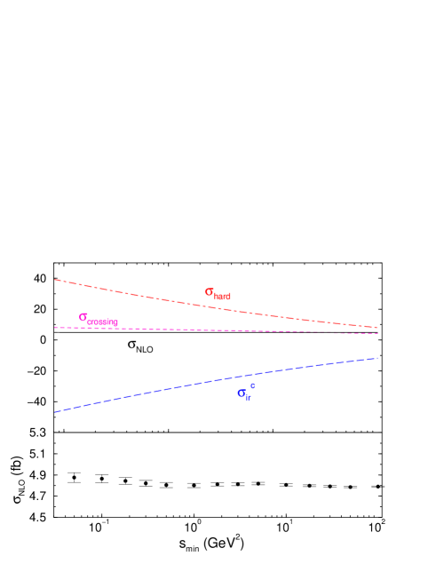
Figure 7: Dependence of $\sigma_{\scriptscriptstyle NLO}(p{\overline{p}}\rightarrow t{\overline{t}}h)$ on the arbitrary cutoff of the one-cutoff PSS method, $s_{min}$, at $\sqrt{s_{\scriptscriptstyle H}}\!=\!2$ TeV, for $M_{h}=120$ GeV, and $\mu=m_{t}$. The upper plot shows the cancellation of the $s_{min}$ dependence between $\sigma_{ir}^{c}$, $\sigma_{crossing}$, and $\sigma_{hard}$. The lower plot shows, on an enlarged scale, the dependence of $\sigma_{\scriptscriptstyle NLO}$ on $s_{min}$, with the corresponding statistical errors.

two-cutoff PSS method

$$\sigma_{\scriptscriptstyle NLO} = \sum_{q\bar{q}}\int dx_{1}dx_{2}{\cal F}_{q}^{p}(x_{1},\mu){\cal F}_{\bar{q}}^{\bar{p}}(x_{2},\mu)\left[\hat{\sigma}^{q\bar{q}}_{\scriptscriptstyle LO}(x_{1},x_{2},\mu)+\hat{\sigma}_{virt}^{q\bar{q}}(x_{1},x_{2},\mu)+\hat{\sigma}_{soft}^{\prime}(x_{1},x_{2},\mu)\right]$$

$$+ \frac{\alpha_{s}}{2\pi}C_{F}\sum_{q\bar{q}}\int dx_{1}dx_{2}\left\{\int_{x_{1}}^{1-\delta_{s}}\frac{dz}{z}\left[{\cal F}_{q}^{p}(\frac{x_{1}}{z},\mu){\cal F}_{\bar{q}}^{\bar{p}}(x_{2},\mu)+{\cal F}_{q}^{\bar{p}}(x_{2},\mu){\cal F}_{\bar{q}}^{p}(\frac{x_{1}}{z},\mu)\right]\right.$$

$$\times\left.\hat{\sigma}_{\scriptscriptstyle LO}^{q\bar{q}}(x_{1},x_{2},\mu)\left[\frac{1+z^{2}}{1-z}\ln\left(\frac{s}{\mu^{2}}\frac{(1-z)^{2}}{z}\frac{\delta_{c}}{2}\right)+1-z\right]+(1\leftrightarrow 2)\right\}$$

$$+ \sum_{q\bar{q}}\int dx_{1}dx_{2}{\cal F}_{q}^{p}(x_{1},\mu){\cal F}_{\bar{q}}^{\bar{p}}(x_{2},\mu)\,\hat{\sigma}_{hard/non-coll}(x_{1},x_{2},\mu)\,\,\,,$$

with

$$\hat{\sigma}_{soft}^{\prime}=\hat{\sigma}_{soft}+\frac{\alpha_{s}}{2\pi}\frac{\Gamma(1-\epsilon)}{\Gamma(1-2\epsilon)}\left(4\pi\right)^{\epsilon}\left(\frac{1}{\epsilon}\right)C_{F}\left[4\ln(\delta_{s})+3\right]\,\,\,,$$ (83)

one-cutoff PSS method

$$\sigma_{\scriptscriptstyle NLO} = \sum_{q\bar{q}}\int dx_{1}dx_{2}{\cal F}_{q}^{p}(x_{1},\mu){\cal F}_{\bar{q}}^{\bar{p}}(x_{2},\mu)\left\{\phantom{\frac{1}{2}}\hat{\sigma}^{q\bar{q}}_{\scriptscriptstyle LO}(x_{1},x_{2},\mu)+\hat{\sigma}_{virt}^{q\bar{q}}(x_{1},x_{2},\mu)\right.$$

$$\left.+\hat{\sigma}_{ir}^{c}(x_{1},x_{2},\mu)+\frac{\alpha_{s}}{2\pi}\,2\,C_{F}\,\hat{\sigma}_{\scriptscriptstyle LO}^{q\bar{q}}(x_{1},x_{2},\mu)\left[\frac{3}{2}\ln\left(\frac{s_{min}}{\mu^{2}}\right)+\frac{\pi^{2}}{3}-\frac{7}{2}\right]\right\}$$

$$+ \frac{\alpha_{s}}{2\pi}C_{F}\sum_{q\bar{q}}\int dx_{1}dx_{2}\left\{\int_{x_{1}}^{1}\frac{dz}{z}\left[{\cal F}_{q}^{p}(\frac{x_{1}}{z},\mu){\cal F}_{\bar{q}}^{\bar{p}}(x_{2},\mu)+{\cal F}_{q}^{\bar{p}}(x_{2},\mu){\cal F}_{\bar{q}}^{p}(\frac{x_{1}}{z},\mu)\right]\right.$$

$$\times\left.\hat{\sigma}_{\scriptscriptstyle LO}^{q\bar{q}}(x_{1},x_{2},\mu)\left[\frac{1+z^{2}}{(1-z)_{+}}\ln\left(\frac{s}{\mu^{2}}\frac{s_{min}}{s}\right)+1-z+(1+z^{2})\left(\frac{\ln\left(1-z\right)}{1-z}\right)_{+}\right]\right.$$

$$\left.+(1\leftrightarrow 2)\phantom{\frac{1}{2}}\right\}+\sum_{q\bar{q}}\int dx_{1}dx_{2}{\cal F}_{q}^{p}(x_{1},\mu){\cal F}_{\bar{q}}^{\bar{p}}(x_{2},\mu)\,\hat{\sigma}_{hard}(x_{1},x_{2},\mu)\,\,\,.$$

We note that $\sigma_{\scriptscriptstyle NLO}$ is finite, since, after mass factorization, both soft and collinear singularities have been canceled between $\hat{\sigma}_{virt}^{q\bar{q}}+\hat{\sigma}_{soft}^{\prime}$ and $\hat{\sigma}_{hard/coll}$ in the two-cutoff PSS method, and between $\hat{\sigma}_{virt}^{q\bar{q}}$ and $\hat{\sigma}_{ir}^{c}$ in the one-cutoff PSS method. The last terms respectively describe the finite real gluon emission of Eq. (27) and Eq. (45). Note that the second term in Eqs. (5) and (5), which is proportional to $\ln\left(\frac{s}{\mu^{2}}\right)$, corresponds exactly to the second and third terms of Eq. (2), as predicted by renormalization group arguments.

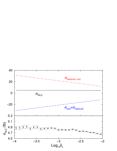
Figure 8: Dependence of $\sigma_{\scriptscriptstyle NLO}(p{\overline{p}}\rightarrow t{\overline{t}}h)$ on the soft cutoff $\delta_{s}$ of the two-cutoff PSS method, at $\sqrt{s_{\scriptscriptstyle H}}\!=\!2$ TeV, for $M_{h}=120$ GeV, $\mu=m_{t}$, and $\delta_{c}=10^{-4}$. The upper plot shows the cancellation of the $\delta_{s}$-dependence between $\sigma_{soft}+\sigma_{hard/coll}$ and $\sigma_{hard/non-coll}$. The lower plot shows, on an enlarged scale, the dependence of $\sigma_{NLO}$ on $\delta_{s}$ with the corresponding statistical errors.

Before we discuss in detail the numerical results for the NLO total cross section for $p\bar{p}\to t\bar{t}h$ we first demonstrate that $\sigma_{\scriptscriptstyle NLO}$ does not depend on the arbitrary cutoffs of the PSS method, i.e. on $s_{min}$ when we use the one-cutoff method, and on the soft and hard/collinear cutoffs $\delta_{s}$ and $\delta_{c}$ when we use the two-cutoff method. We note that the cancellation of the cutoff dependence at the level of the total NLO cross section is a very delicate issue, since it involves both analytical and numerical contributions. It is crucial to study the behavior of $\sigma_{NLO}$ in a region where the cutoff(s) are small enough to justify the approximations used in the analytical calculation of the IR-divergent part of $\hat{\sigma}_{real}^{q\bar{q}}$, but not so small to give origin to numerical instabilities.

Fig. 7 is about the one-cutoff PSS method and shows the dependence of $\sigma_{\scriptscriptstyle NLO}$ on $s_{min}$. In the upper window we illustrate the cancellation of the $s_{min}$ dependence between $\sigma_{ir}^{c}$, $\sigma_{crossing}$, and $\sigma_{hard}$, while in the lower window we show, on a larger scale, the behavior of ${\sigma}_{\scriptscriptstyle NLO}$ including the statistical errors from the Monte-Carlo integration. We note that $\sigma_{\scriptscriptstyle NLO}$ also includes the Born cross section and the virtual contribution to the NLO cross section, which are both $s_{min}$-independent, and are therefore not shown explicitly in the upper part of Fig. 7. Clearly a plateau is reached in the region $0.1\,\mathrm{GeV}^{2}<s_{min}<100\,\mathrm{GeV}^{2}$.

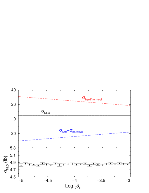
Figure 9: Dependence of $\sigma_{\scriptscriptstyle NLO}(p{\overline{p}}\rightarrow t{\overline{t}}h)$ on the collinear cutoff $\delta_{c}$ of the two-cutoff PSS method, at $\sqrt{s_{\scriptscriptstyle H}}\!=\!2$ TeV, for $M_{h}=120$ GeV, $\mu=m_{t}$, and $\delta_{s}=5\times 10^{-4}$. The upper plot shows the cancellation of the $\delta_{c}$-dependence between $\sigma_{soft}+\sigma_{hard/coll}$ and $\sigma_{hard/non-coll}$. The lower plot shows, on an enlarged scale, the dependence of $\sigma_{NLO}$ on $\delta_{c}$ with the corresponding statistical errors.

Figs. 8 and 9 are about the two-cutoff PSS method. In Fig. 8, we show the dependence of $\sigma_{\scriptscriptstyle NLO}$ on the soft cutoff, $\delta_{s}$, for a fixed value of the hard/collinear cutoff, $\delta_{c}\!=\!10^{-4}$. In Fig. 9, we show the dependence of $\sigma_{\scriptscriptstyle NLO}$ on the hard/collinear cutoff, $\delta_{c}$, for a fixed value of the soft cutoff, $\delta_{s}\!=\!5\times 10^{-4}$. In the upper window of Fig. 8(9) we illustrate the cancellation of the $\delta_{s}$($\delta_{c}$) dependence between ${\sigma}_{soft}+{\sigma}_{hard/coll}$ and ${\sigma}_{hard/non-coll}$, while in the lower window we show, on a larger scale, ${\sigma}_{\scriptscriptstyle NLO}$ with the statistical errors from the Monte-Carlo integration. As before, $\sigma_{\scriptscriptstyle NLO}$ also includes the contribution from the Born and the virtual cross sections, which are both cutoff-independent and are not shown explicitly in the upper parts of Figs. 8,9. For $\delta_{s}$ in the range $10^{-4}-2.5\times 10^{-3}$ and $\delta_{c}$ in the range $10^{-5}-10^{-3}$, a clear plateau is reached and the NLO total cross section is independent of the technical cutoffs of the two-cutoff PSS method. All the results presented in the following are obtained using the two-cutoff PSS method with $\delta_{s}$ and $\delta_{c}$ in the range $10^{-4}\!-\!10^{-3}$. We have confirmed them using the one-cutoff PSS method with $1\!\leq\!s_{min}\!\leq\!10$.

6 Numerical results

In the following we discuss in detail our results for the NLO inclusive total cross section for $p{\overline{p}}\rightarrow t{\overline{t}}h$, $\sigma_{\scriptscriptstyle NLO}(p{\overline{p}}\rightarrow t{\overline{t}}h)$, as introduced in Sect. 2 and explicitly given by Eqs. (5) and (5). Our numerical results are found using CTEQ4M parton distribution functions  [33] and the 2-loop evolution of $\alpha_{s}(\mu)$ for the calculation of the NLO cross section, and CTEQ4L parton distribution functions and the 1-loop evolution of $\alpha_{s}(\mu)$ for the calculation of the lowest order cross section, unless stated otherwise. The top-quark mass is taken to be $m_{t}\!=\!174$ GeV and $\alpha_{s}^{\scriptscriptstyle NLO}(M_{Z})\!=\!0.116$.

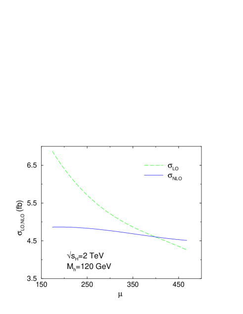
Figure 10: Dependence of $\sigma_{\scriptscriptstyle LO,NLO}(p{\overline{p}}\rightarrow t{\overline{t}}h)$ on the renormalization/factorization scale $\mu$, at $\sqrt{s_{\scriptscriptstyle H}}\!=\!2$ TeV, for $M_{h}\!=\!120$ GeV.

First of all, in Fig. 10 we show how at NLO the dependence on the arbitrary renormalization/factorization scale $\mu$ is significantly reduced. We use $M_{h}\!=\!120$ GeV for illustration purposes. We note that only for scales $\mu$ of the order of $2m_{t}+M_{h}$ or bigger is the NLO result greater than the lowest order result at $\sqrt{s_{\scriptscriptstyle H}}=2$ TeV.

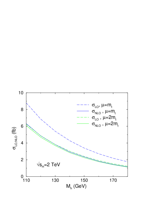
Figure 11: $\sigma_{\scriptscriptstyle NLO}$ and $\sigma_{\scriptscriptstyle LO}$ for $p{\overline{p}}\rightarrow t{\overline{t}}h$ as functions of $M_{h}$, at $\sqrt{s_{\scriptscriptstyle H}}\!=\!2$ TeV, for $\mu\!=m_{t}$ and $\mu\!=\!2m_{t}$.

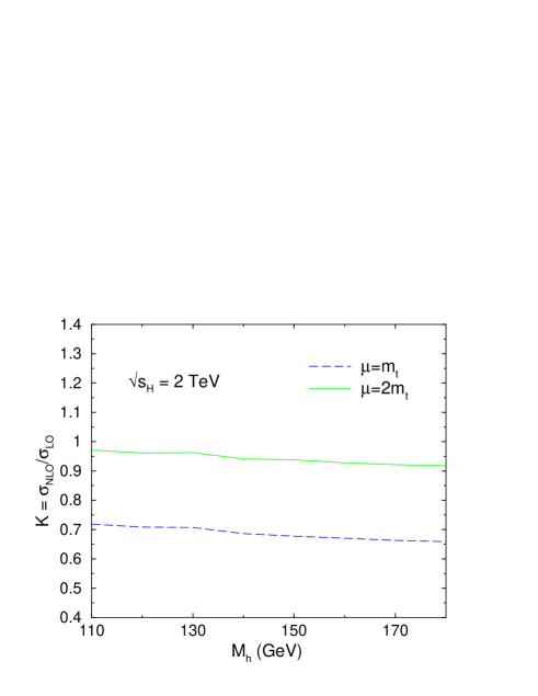
Figure 12: K-factor for $p{\overline{p}}\rightarrow t{\overline{t}}h$ as a function of $M_{h}$, at $\sqrt{s_{\scriptscriptstyle H}}\!=\!2$ TeV, for $\mu\!=m_{t}$ and $\mu\!=\!2m_{t}$ .

Fig. 11 shows both the LO and the NLO total cross section for $p\bar{p}\rightarrow t\bar{t}h$ as a function of $M_{h}$, at $\sqrt{s_{\scriptscriptstyle H}}\!=\!2$ TeV, for two values of the renormalization/factorization scale, $\mu\!=\!m_{t}$ and $\mu\!=\!2m_{t}$. Over the entire range of $M_{h}$ accessible at the Tevatron, the NLO corrections decrease the rate for renormalization/factorization scales $\mu<2m_{t}+M_{h}$. The reduction is much less dramatic at $\mu\!=\!2m_{t}$ than at $\mu\!=\!m_{t}$, as can be seen from both Fig. 10 and Fig. 11. An illustrative sample of results is also given in Table 1. The error we quote on our values is the statistical error of the numerical integration involved in evaluating the total cross section. We estimate the remaining theoretical uncertainty on the NLO results to be of the order of $12\%$. This is mainly due to: the left over $\mu$-dependence (about $8\%$), the dependence on the PDFs (about $6\%$), and the error on $m_{t}$ (about $7\%$) which particularly plays a role in the Yukawa coupling.

$M_{h}$ (GeV)	$\mu$	$\sigma_{\scriptscriptstyle LO}$ (fb)	$\bar{\sigma}_{\scriptscriptstyle LO}$ (fb)	$\sigma_{\scriptscriptstyle NLO}$ (fb)
	$m_{t}$	6.8662 $\pm$ 0.0013	5.2843 $\pm$ 0.0008	4.863 $\pm$ 0.029
120	$m_{t}+M_{h}/2$	5.9085 $\pm$ 0.0011	4.5846 $\pm$ 0.0007	4.847 $\pm$ 0.024
	$2m_{t}$	4.8789 $\pm$ 0.0009	3.8252 $\pm$ 0.0006	4.691 $\pm$ 0.020
	$2m_{t}+M_{h}$	4.2548 $\pm$ 0.0008	3.3600 $\pm$ 0.0005	4.511 $\pm$ 0.017
	$m_{t}$	3.4040 $\pm$ 0.0006	2.5811 $\pm$ 0.0005	2.355 $\pm$ 0.013
150	$m_{t}+M_{h}/2$	2.8289 $\pm$ 0.0005	2.1668 $\pm$ 0.0004	2.315 $\pm$ 0.011
	$2m_{t}$	2.4007 $\pm$ 0.0004	1.8553 $\pm$ 0.0004	2.253 $\pm$ 0.010
	$2m_{t}+M_{h}$	2.0282 $\pm$ 0.0004	1.5813 $\pm$ 0.0003	2.147 $\pm$ 0.008
	$m_{t}$	1.7605 $\pm$ 0.0003	1.3153 $\pm$ 0.0002	1.160 $\pm$ 0.007
180	$m_{t}+M_{h}/2$	1.4142 $\pm$ 0.0003	1.0693 $\pm$ 0.0002	1.158 $\pm$ 0.005
	$2m_{t}$	1.2326 $\pm$ 0.0002	0.9390 $\pm$ 0.0001	1.132 $\pm$ 0.004
	$2m_{t}+M_{h}$	1.0096 $\pm$ 0.0002	0.7773 $\pm$ 0.0001	1.069 $\pm$ 0.004

Table 1: Values of both $\sigma_{\scriptscriptstyle LO}$ (calculated with LO $\alpha_{s}(\mu)$ and LO PDFs), $\bar{\sigma}_{\scriptscriptstyle LO}$ (calculated with NLO $\alpha_{s}(\mu)$ and NLO PDFs), and $\sigma_{\scriptscriptstyle NLO}$ for different values of $M_{h}$ and for different renormalization/factorization scales $\mu$.

The corresponding K-factor, i.e. the ratio of the NLO cross section to the LO one,

$$K=\frac{\sigma_{\scriptscriptstyle NLO}}{\sigma_{\scriptscriptstyle LO}}\;,$$ (85)

is shown in Fig. 12. For scales $\mu$ between $\mu\!=\!m_{t}$ and $\mu\!=\!2m_{t}$, the K-factor varies roughly between $K\!=\!0.70$ and $K\!=\!0.95$, when $M_{h}$ varies in the range between $100$ and $200$ GeV. For scales of the order of $\mu\!=\!2m_{t}+M_{h}$ the K-factor is of order one and becomes larger than one for higher scales. Given the strong scale dependence of the LO cross section, the K-factor also shows a significant $\mu$-dependence and therefore is an equally unreliable prediction. Moreover it is important to remember that the K-factor depends on how the LO cross section is calculated. We choose to calculate the LO cross section using both LO $\alpha_{s}(\mu)$ and LO PDFs, denoted by $\sigma_{\scriptscriptstyle LO}$ in Table 1. An equally valid approach could be to evaluate the LO cross section using NLO $\alpha_{s}(\mu)$ and NLO PDFs, denoted by ${\bar{\sigma}}_{\scriptscriptstyle LO}$ in Table 1, in which case the K-factor would just represent the impact of the ${\cal O}(\alpha_{s})$ corrections that do not originate from the running of $\alpha_{s}(\mu)$ and the PDFs. Since $\sigma_{\scriptscriptstyle LO}\!>\!\bar{\sigma}_{\scriptscriptstyle LO}$, the K-factor obtained using $\sigma_{\scriptscriptstyle LO}$ is smaller than the one obtained using $\bar{\sigma}_{\scriptscriptstyle LO}$, and it is important to match the right K-factor to the right $\sigma_{\scriptscriptstyle LO}$ or $\bar{\sigma}_{\scriptscriptstyle LO}$. Therefore we would like to stress once more that we only discuss the K-factor as a qualitative indication of the impact of ${\cal O}(\alpha_{s})$ QCD corrections, for different processes or when using different approaches. The physical meaningful quantity is the NLO cross section, not the K-factor.

For comparison, we have estimated the K-factor also in the EHA [9], and we obtain $K\!\simeq\!0.6-0.7$, for Higgs boson masses up to 150 GeV and renormalization/factorization scales in the range between $\mu\!=\!m_{t}$ and $\mu\!=\!2m_{t}+M_{h}$. As anticipated, we do not expect the EHA to give a quantitatively good approximation of the full $p\bar{p}\rightarrow t\bar{t}h$ calculation at ${\cal O}(\alpha_{s})$, since at $\sqrt{s_{\scriptscriptstyle H}}\!=\!2$ TeV and for a SM Higgs boson above the experimental bound, we cannot work in the limit $M_{h},m_{t}/\sqrt{s}\!\ll\!1$ or $M_{h}/m_{t}\!\ll\!1$. Still the EHA gives a remarkably good qualitative indication of the fact that the first order QCD corrections may lower the LO total cross section.

It is interesting to compare our NLO result for $p\bar{p}\rightarrow t{\overline{t}}h$ with the NLO result for $p{\overline{p}}\rightarrow t{\overline{t}}$. Since the Higgs boson is colorless, one would naively expect the QCD corrections to both processes to be of roughly the same size. Defining the NLO cross section using the NLO evolution of $\alpha_{s}(\mu)$ and the NLO CTEQ4M PDFs, and the LO cross section using the LO evolution of $\alpha_{s}(\mu)$ and the LO CTEQ4L PDFs, the K-factor for $t{\overline{t}}$ production at $\sqrt{s_{\scriptscriptstyle H}}\!=\!2$ TeV, with $\mu\!=\!m_{t}$ and $m_{t}\!=\!174$ GeV, is:

$$K(p{\overline{p}}\rightarrow t{\overline{t}})\mid_{q\overline{q}} = 0.98\,\,\,,$$

$$K(p{\overline{p}}\rightarrow t{\overline{t}})\mid_{tot} = 1.05\;,$$ (86)

where the $q{\overline{q}}$ label indicates that only the $q{\overline{q}}$ initial state is included. The size of the QCD corrections to $p{\overline{p}}\rightarrow t{\overline{t}}$ is thus similar in magnitude to the result obtained in Fig. 12, taking into account that $p\bar{p}\rightarrow t\bar{t}h$ is completely dominated by the $q\bar{q}$ channel. Of course, we do not expect a better agreement, since in $p\bar{p}\rightarrow t\bar{t}h$ an additional heavy particle is produced, and new contributions to the virtual corrections arise. Moreover, taking the EHA as an indication, one could naively expect that the radiation of a Higgs boson introduces an additional negative contribution. We also observe that, if we now use as LO cross section the one obtained using NLO $\alpha_{s}(\mu)$ and NLO CTEQ4M PDFs, the two K-factors in Eq. (6) increase, according to the comment we made above, and become:

$$K(p{\overline{p}}\rightarrow t{\overline{t}})\mid_{q\overline{q}} = 1.18\,\,\,,$$

$$K(p{\overline{p}}\rightarrow t{\overline{t}})\mid_{tot} = 1.24\;,$$ (87)

in agreement with the literature [34]. Moreover, since the NLO cross section for $p\bar{p}\rightarrow t\bar{t}$ is further increased by the resummation of the leading and next-to-leading logarithms arising from the threshold region dynamics, the total K-factor for $p\bar{p}\rightarrow t\bar{t}$ can be as high as 1.33 for $\mu\!=\!m_{t}$. With this respect, we also note that, contrary to $p\bar{p}\rightarrow t\bar{t}$, in the threshold region for $p\bar{p}\rightarrow t\bar{t}h$ there are large negative contributions, mainly from soft gluon radiation, which are largely compensated by large positive contributions from hard gluon radiation at larger $\sqrt{s}$. In the threshold region the Coulomb term, coming from the exchange of virtual gluons between the $t/\bar{t}$ external legs, is important and contributes to decrease the NLO cross section, although it is moderated by the behavior of the three-body phase space. In the strict threshold limit, the Coulomb contribution to $p\bar{p}\to t\bar{t}h$ goes to zero, while for $t\bar{t}$ production it is constant and dominates the NLO cross section.

7 Conclusion

The NLO inclusive total cross section for the Standard Model process $p{\overline{p}}\rightarrow t{\overline{t}}h$ at $\sqrt{s}_{H}\!=\!2$ TeV shows a significantly reduced scale dependence as compared to the Born result and leads to increased confidence in predictions based on these results. The NLO QCD corrections slightly decrease or increase the Born level cross section depending on the renormalization/factorization scales used. The NLO inclusive total cross section for Higgs boson masses in the range accessible at the Tevatron, $120\!<\!M_{h}\!<\!180$ GeV, is of the order of $1-5$ fb.

The contributions to the NLO cross section resulting from real gluon emission have been calculated in two variations of the phase space slicing method, involving one or two arbitrary numerical cutoff parameters, respectively. This is the first application of the one-cutoff phase space slicing approach, (“$s_{min}$”), to a cross section involving more than one massive particle in the final state. The correspondence between the two phase space slicing approaches is made explicit. The virtual contributions to the NLO cross section require the calculation of both box and pentagon diagrams involving several massive particles and explicit results for the integrals have been presented in the appendices. These techniques can now be applied to other similar processes.

Appendix A Pentagon scalar integrals

In this appendix we review the details of the calculation of the pentagon scalar integrals that appear in the calculation of diagrams $P_{1}$ and $P_{2}$ illustrated in Fig. 5. Using the momentum flow and the notation shown in Fig. 5, the pentagon scalar integral originating from diagram $P_{1}$ ($E0_{p1}$) can be written as:

$$E0_{p1}=\mu^{4-d}\int\frac{d^{d}k}{(2\pi)^{d}}\frac{1}{N_{1}N_{2}N_{3}N_{4}N_{5}}\,\,\,,$$ (88)

where

$$N_{1} = k^{2}\,\,\,,$$ (89)

$$N_{2} = (k+q_{1})^{2}\,\,\,,$$

$$N_{3} = (k+q_{1}+q_{2})^{2}\,\,\,,$$

$$N_{4} = (k+q_{1}+q_{2}-p_{t}^{\prime})^{2}-m_{t}^{2}\,\,\,,$$

$$N_{5} = (k+q_{1}+q_{2}-p_{t}^{\prime}-p_{h})^{2}-m_{t}^{2}\,\,\,.$$

We note that we included a factor $\mu^{4-d}$ in the definition of the $d$-dimensional scalar integrals in order to have them in the most convenient form for the calculation of the virtual amplitude squared. The pentagon scalar integral originating from diagram $P_{2}$, $E0_{p2}$, can be obtained from Eqs.(88) and (89) by exchanging $q_{1}\leftrightarrow q_{2}$. Therefore in the following we limit our discussion to $E0_{p1}$, the generalization to $E0_{p2}$ being straightforward.

We calculate these integrals following the method introduced by the authors of Ref. [11]. To make contact with their notation, we denote by $k_{i}$ the external momenta (such that $k_{i}^{2}\!=\!m_{i}^{2}$), by $M_{i}$ the internal masses, by $p_{i}$ the sum of the first $i$ external momenta, $p_{i}^{\mu}\!=\!\sum_{j=1}^{i}k_{j}^{\mu}$, by $p_{ij}$ the difference $p_{ij}^{\mu}\!=\!p_{j-1}^{\mu}-p_{i-1}^{\mu}=k_{i}^{\mu}+k_{i+1}^{\mu}+\cdots+k_{j-1}^{\mu}$ (for $i<j$), and finally by ${\bar{s}}_{ij}$ the invariant masses ${\bar{s}}_{ij}\!=\!(k_{i}+k_{j})^{2}$.

The topology of the generic pentagon scalar integral is illustrated in Fig. 13, which can be specified to our case by identifying:

$$k_{1} \longrightarrow -q_{1}\,\,\,\,(\mbox{incoming}\,\,q)$$

$$k_{2} \longrightarrow -q_{2}\,\,\,\,(\mbox{incoming}\,\,\bar{q})$$

$$k_{3} \longrightarrow p_{t}^{\prime}\,\,\,\,(\mbox{outgoing}\,\,\bar{t})$$ (90)

$$k_{4} \longrightarrow p_{h}\,\,\,\,(\mbox{outgoing}\,\,h)$$

$$k_{5} \longrightarrow p_{t}\,\,\,\,(\mbox{outgoing}\,\,t)\;.$$

Figure 13: Topology of the pentagon scalar integral

Using the standard Feynman parameterization technique, the pentagon integral in Eq.(88) can be written as:

$$E0_{p1}=-{i\over 16\pi^{2}}(4\pi\mu^{2})^{\epsilon}\Gamma(3+\epsilon)\int_{0}^{1}{\Pi_{i=1}^{5}da_{i}\delta(1-\Sigma_{i=1}^{5}a_{i})\over[{\cal D}_{p1}(a_{i})]^{3+\epsilon}}\,\,\,,$$ (91)

where the denominator ${\cal D}_{p1}(a_{i})$ is:

$${\cal D}_{p1}(a_{i})=\sum_{i,j=1}^{5}S_{ij}a_{i}a_{j}-i\eta\,\,\,,$$ (92)

and the symmetric matrix $S_{ij}$ is given by:

$$S_{ij}=\frac{1}{2}(M_{i}^{2}+M_{j}^{2}-p_{ij}^{2})\,\,\,.$$ (93)

For our particular process, the matrix $S_{ij}$ has the following explicit form:

$$S=\frac{1}{2}\left(\begin{array}[]{c c c c c}0&0&-{\bar{s}}_{12}&(m_{t}^{2}-{\bar{s}}_{45})&0\\ 0&0&0&(m_{t}^{2}-{\bar{s}}_{23})&(m_{t}^{2}-{\bar{s}}_{15})\\ -{\bar{s}}_{12}&0&0&0&(m_{t}^{2}-{\bar{s}}_{34})\\ (m_{t}^{2}-{\bar{s}}_{45})&(m_{t}^{2}-{\bar{s}}_{23})&0&2m_{t}^{2}&(2m_{t}^{2}-M_{h}^{2})\\ 0&(m_{t}^{2}-{\bar{s}}_{15})&(m_{t}^{2}-{\bar{s}}_{34})&(2m_{t}^{2}-M_{h}^{2})&2m_{t}^{2}\end{array}\right)\,\,\,.$$ (94)

Following Ref. [11], $E0_{p1}$ can then be written as the linear combination of five scalar box integrals $D0_{p1}^{(i)}$:

$$E0_{p1}=-\frac{1}{2}\sum_{i=1}^{5}c_{i}D0_{p1}^{(i)}\,\,\,,$$ (95)

where each $D0_{p1}^{(i)}$ scalar box integral can be obtained from the scalar pentagon integral $E0_{p1}$ of Eq. (91) in the limit where one of the Feynman parameters $a_{i}$ of the internal propagators goes to zero (i.e. $D0_{p1}^{(i)}$ is obtained when $a_{i}\rightarrow 0$). The five box scalar integrals we need are given in Secs. A.1-A.5. The coefficients $c_{i}$ in Eq. (95) are given by:

$$c_{i}=\sum_{j=1}^{5}S_{ij}^{-1}\,\,\,.$$ (96)

Using Eq. (94) we can easily obtain them in terms of $m_{t}$, $M_{h}$, and the kinematic invariants ${\bar{s}}_{ij}$.

The final result for the pentagon scalar integral $E0_{p1}$ can be written as:

$$E0_{p1}=\frac{i}{16\pi^{2}}{\cal N}_{t}\biggl{[}{X_{-2}\over\epsilon^{2}}+{X_{-1}\over\epsilon}+X_{0}\biggr{]}\,\,\,,$$ (97)

where ${\cal N}_{t}$ is given in Eq. (13), while $X_{-2}$, $X_{-1}$ and $X_{0}$ are obtained using Eqs. (95)-(94), and the results in Secs. A.1-A.5. The expression for $X_{0}$ is too lengthy to be given explicitly in this appendix, while $X_{-2}$ and $X_{-1}$ have the following compact form:

$$X_{-2} = \frac{1}{2\sigma}\left(-\frac{1}{\omega_{1}\tau_{1}}-\frac{1}{\omega_{2}\tau_{2}}+\frac{2}{\tau_{1}\tau_{2}}\right)\,\,\,,$$ (98)

$$X_{-1} = \frac{1}{\sigma\tau_{1}\tau_{2}}\left(-\Lambda_{\sigma}+\Lambda_{\omega_{1}}+\Lambda_{\omega_{2}}-\Lambda_{\tau_{1}}-\Lambda_{\tau_{2}}\right)+\frac{1}{\sigma\tau_{2}\omega_{2}}\left(\Lambda_{\tau_{2}}-\Lambda_{\tau_{1}}+\Lambda_{\omega_{2}}\right)+$$

$$+ \frac{1}{\sigma\tau_{1}\omega_{1}}\left(\Lambda_{\tau_{1}}-\Lambda_{\tau_{2}}+\Lambda_{\omega_{1}}\right)\,\,\,,$$

where we have defined:

$$\sigma = (q_{1}+q_{2})^{2}=s\,\,\,,$$ (99)

$$\tau_{1} = m_{t}^{2}-(q_{1}-p_{t})^{2}=2\,q_{1}\cdot p_{t}=s_{qt}\,\,\,,$$

$$\tau_{2} = m_{t}^{2}-(q_{2}-p_{t}^{\prime})^{2}=2\,q_{2}\cdot p_{t}^{\prime}=s_{\bar{q}\bar{t}}\,\,\,,$$

$$\omega_{1} = (p_{t}+p_{h})^{2}-m_{t}^{2}\,\,\,,$$

$$\omega_{2} = (p_{t}^{\prime}+p_{h})^{2}-m_{t}^{2}\,\,\,,$$

and

$$\Lambda_{\sigma} = \ln\left(\frac{\sigma}{m_{t}^{2}}\right)\,\,\,\,,\,\,\,\,\Lambda_{\tau_{1}}=\ln\left(\frac{\tau_{1}}{m_{t}^{2}}\right)\,\,\,\,,\,\,\,\,\Lambda_{\tau_{2}}=\ln\left(\frac{\tau_{2}}{m_{t}^{2}}\right)\,\,\,\,,$$ (100)

$$\Lambda_{\omega_{1}} = \ln\left(\frac{\omega_{1}}{m_{t}^{2}}\right)\,\,\,\,,\,\,\,\,\Lambda_{\omega_{2}}=\ln\left(\frac{\omega_{2}}{m_{t}^{2}}\right)\,\,\,\,.$$

We discuss in the following the box scalar integrals $D0_{p1}^{(i)}$, which are used in Eq. (95) to calculate $E0_{p1}$. The analogous box scalar integrals for $E0_{p2}$ can be obtained from the $D0_{p1}^{(i)}$ by exchanging $q_{1}\leftrightarrow q_{2}$ in their analytic expression.

A.1 Box scalar integral $D0_{p1}^{(1)}$

$D0_{p1}^{(1)}$ is obtained from the pentagon in the limit $a_{1}\rightarrow 0$ and corresponds to the following integral:

$$D0_{p1}^{(1)} = \mu^{4-d}\int\frac{d^{d}k}{(2\pi)^{d}}\frac{1}{N_{2}N_{3}N_{4}N_{5}}$$

$$= \mu^{4-d}\int\frac{d^{d}k}{(2\pi)^{d}}\frac{1}{k^{2}(k+q_{2})^{2}[(k+q_{2}-p_{t}^{\prime})^{2}-m_{t}^{2}][(k+q_{2}-p_{t}^{\prime}-p_{h})^{2}-m_{t}^{2}]}\,\,\,,$$

after the momentum shift $k\rightarrow k-q_{1}$ has been applied to the denominators listed in Eq.(89). The part of $D0_{p1}^{(1)}$ which contributes to the virtual amplitude squared is given by:

$$D0_{p1}^{(1)}=\frac{i}{16\pi^{2}}{\cal N}_{t}\left(-\frac{1}{\omega_{2}\tau_{2}}\right)\left(\frac{X_{-2}}{\epsilon^{2}}+\frac{X_{-1}}{\epsilon}+X_{0}\right)\,\,\,,$$ (102)

where ${\cal N}_{t}$ is given in Eq. (13), while the coefficients $X_{-2}$, $X_{-1}$, and $X_{0}$ are given by:

$$X_{-2} = \frac{1}{2}\,\,\,,$$ (103)

$$X_{-1} = \ln\left(\frac{\tau_{1}m_{t}^{2}}{\omega_{2}\tau_{2}}\right)\,\,\,,$$

$$X_{0} = Re\left\{-\frac{5}{6}\pi^{2}+\ln^{2}\left(\frac{\omega_{2}}{m_{t}^{2}}\right)+\ln^{2}\left(\frac{\tau_{2}}{m_{t}^{2}}\right)-\ln^{2}\left(\frac{\tau_{1}}{m_{t}^{2}}\right)\right.$$

$$+ 2\,\ln\left(\frac{\omega_{2}+\tau_{1}}{\tau_{2}}\right)\ln\left(\frac{\tau_{1}}{\omega_{2}}\right)+2\,\ln\left(\frac{\tau_{2}-\tau_{1}}{\omega_{2}}\right)\ln\left(\frac{\tau_{1}}{\tau_{2}}\right)$$

$$- 2\left.\,\mbox{Li}_{2}\left(\frac{\tau_{2}-\tau_{1}-\omega_{2}}{\tau_{2}}\right)-2\,\mbox{Li}_{2}\left(\frac{\omega_{2}+\tau_{1}-\tau_{2}}{\omega_{2}}\right)+2\,\mbox{Li}_{2}\left(\frac{\tau_{1}(\omega_{2}+\tau_{1}-\tau_{2})}{\omega_{2}\tau_{2}}\right)-{\cal I}_{0}\right\}\,\,\,,$$

where

$${\cal I}_{0} = \ln\left(\frac{\tau_{2}}{\tau_{1}}\right)\ln\left(\frac{M_{h}^{2}}{m_{t}^{2}}\right)+\left\{-\mbox{Li}_{2}\left(\frac{1}{\lambda_{+}}\right)+\ln\left(\frac{\tau_{2}}{\tau_{1}}\right)\ln\left(\frac{-\tau_{1}-\lambda_{+}(\tau_{2}-\tau_{1})}{\tau_{2}-\tau_{1}}\right)\right.$$ (105)

$$- \left.\mbox{Li}_{2}\left(\frac{\tau_{2}}{\lambda_{+}(\tau_{2}-\tau_{1})+\tau_{1}}\right)+\mbox{Li}_{2}\left(\frac{\tau_{1}}{\lambda_{+}(\tau_{2}-\tau_{1})+\tau_{1}}\right)+(\lambda_{+}\leftrightarrow\lambda_{-})\right\}\,\,\,,$$

and

$$\lambda_{\pm}=\frac{1}{2}\left(1\pm\sqrt{1-\frac{4m_{t}^{2}}{M_{h}^{2}}}\right)\,\,\,.$$ (106)

A.2 Box scalar integral $D0_{p1}^{(2)}$

$D0_{p1}^{(2)}$ is obtained from the pentagon in the limit $a_{2}\rightarrow 0$ and corresponds to the following integral:

$$D0_{p1}^{(2)} = \mu^{4-d}\int\frac{d^{d}k}{(2\pi)^{d}}\frac{1}{N_{1}N_{3}N_{4}N_{5}}$$

$$= \mu^{4-d}\int\frac{d^{d}k}{(2\pi)^{d}}\frac{1}{k^{2}(k+q)^{2}[(k+q-p_{t}^{\prime})^{2}-m_{t}^{2}][(k+q-p_{t}^{\prime}-p_{h})^{2}-m_{t}^{2}]}\,\,\,.$$

$D0_{p2}^{(2)}$ is equal to $D0_{p1}^{(2)}$, and they both coincide with $D0_{b1}$ in Appendix B.1.

A.3 Box scalar integral $D0_{p1}^{(3)}$

$D0_{p1}^{(3)}$ is obtained from the pentagon in the limit $a_{3}\rightarrow 0$ and corresponds to the following integral:

$$D0_{p1}^{(3)} = \mu^{4-d}\int\frac{d^{d}k}{(2\pi)^{d}}\frac{1}{N_{1}N_{2}N_{4}N_{5}}$$

$$= \mu^{4-d}\int\frac{d^{d}k}{(2\pi)^{d}}\frac{1}{k^{2}(k+q_{1})^{2}[(k+q_{1}-p_{t})^{2}-m_{t}^{2}][(k+q_{1}-p_{t}-p_{h})^{2}-m_{t}^{2}]}\,\,\,,$$

after the momentum shift $k\rightarrow-k-q_{1}$ has been applied to the denominators in Eq. (89). We notice that this integral can be obtained from $D0_{p1}^{(1)}$ when $q_{2}\rightarrow q_{1}$ and $p_{t}^{\prime}\rightarrow p_{t}$.

A.4 Box scalar integral $D0_{p1}^{(4)}$

$D0_{p1}^{(4)}$ is obtained from the pentagon in the limit $a_{4}\rightarrow 0$ and corresponds to the following integral:

$$D0_{p1}^{(4)} = \mu^{4-d}\int\frac{d^{d}k}{(2\pi)^{d}}\frac{1}{N_{1}N_{2}N_{3}N_{5}}$$

$$= \mu^{4-d}\int\frac{d^{d}k}{(2\pi)^{d}}\frac{1}{k^{2}(k+q_{2})^{2}(k+q_{1}+q_{2})^{2}[(k+q_{1}+q_{2}-p_{t})^{2}-m_{t}^{2}]}\,\,\,,$$

after the momentum shift $k\rightarrow-k-q_{1}-q_{2}$ has been applied to the denominators in Eq. (89). This integral coincides with $D0_{b3}^{(3)}$ in Appendix B.3.

A.5 Box scalar integral $D0_{p1}^{(5)}$

$D0_{p1}^{(5)}$ is obtained from the pentagon in the limit $a_{5}\rightarrow 0$ and corresponds to the following integral:

$$D0_{p1}^{(5)} = \mu^{4-d}\int\frac{d^{d}k}{(2\pi)^{d}}\frac{1}{N_{1}N_{2}N_{3}N_{4}}$$

$$= \mu^{4-d}\int\frac{d^{d}k}{(2\pi)^{d}}\frac{1}{k^{2}(k+q_{1})^{2}(k+q_{1}+q_{2})^{2}[(k+q_{1}+q_{2}-p_{t}^{\prime})^{2}-m_{t}^{2}]}$$

This integral coincides with $D0_{b3}^{(1)}$ in Appendix B.3.

Appendix B Box scalar integrals

B.1 Box 1 : box scalar integral $D0_{b1}$

The scalar box integral $D0_{b1}$ can be written as:

$$D0_{b1}=\mu^{4-d}\int\frac{d^{d}k}{(2\pi)^{d}}\frac{1}{N_{1}N_{2}N_{3}N_{4}}\,\,\,,$$ (111)

where

$$N_{1} = k^{2}\,\,\,,$$

$$N_{2} = (k+q)^{2}\,\,\,,$$ (112)

$$N_{3} = (k+q-p_{t}^{\prime})^{2}-m_{t}^{2}\,\,\,,$$

$$N_{4} = (k+q-p_{t}^{\prime}-p_{h})^{2}-m_{t}^{2}\,\,\,.$$

The analytical expression for this integral can be found in Ref. [35]. Since the integral is finite, we have evaluated it in $d=4$ dimensions using the FF package [24].

B.2 Box 2: box scalar integrals $D0_{b2}^{(1)}$ and $D0_{b2}^{(2)}$

The scalar box integral $D0_{b2}^{(1)}$ can be written as:

$$D0_{b2}^{(1)}=\mu^{4-d}\int\frac{d^{d}k}{(2\pi)^{d}}\frac{1}{N_{1}N_{2}N_{3}N_{4}}\,\,\,,$$ (113)

where

$$N_{1} = k^{2}\,\,\,,$$

$$N_{2} = (k+p_{t})^{2}-m_{t}^{2}\,\,\,,$$

$$N_{3} = (k+p_{t}+p_{h})^{2}-m_{t}^{2}\,\,\,,$$

$$N_{4} = (k-p_{t}^{\prime})^{2}-m_{t}^{2}\,\,\,,$$ (114)

while $D0_{b2}^{(2)}$ is obtained from $D0_{b2}^{(1)}$ by exchanging $p_{t}\leftrightarrow p_{t}^{\prime}$. Therefore, all the following results for $D0_{b2}^{(1)}$ can be easily extended to $D0_{b2}^{(2)}$.

The part of $D0_{b2}^{(1)}$ which contributes to the virtual amplitude squared is of the form:

$$D0_{b2}^{(1)}=\frac{i}{16\pi^{2}}{\cal N}_{t}\left({X_{-1}\over\epsilon}+X_{0}\right){1\over(m_{t}^{2}-{\bar{s}}_{th}){\bar{s}}_{t\bar{t}}\beta_{t\bar{t}}}\,\,\,,$$ (115)

where ${\cal N}_{t}$ is given in Eq. (13), while ${\bar{s}}_{t\bar{t}}=(p_{t}+p_{t}^{\prime})^{2}=(q-p_{h})^{2}>0$, $\beta_{t\bar{t}}=\sqrt{1-{4m_{t}^{2}\over{\bar{s}}_{t\bar{t}}}}$, ${\bar{s}}_{th}=(p_{t}+p_{h})^{2}$. The pole part $X_{-1}$ is:

$$X_{-1}=\ln\left(\frac{1+\beta_{t\bar{t}}}{1-\beta_{t\bar{t}}}\right)\,\,\,,$$ (116)

while the finite part can be calculated using Ref. [36].

B.3 Box 3: box scalar integrals $D0_{b3}^{(1)}$, $D0_{b3}^{(2)}$, $D0_{b3}^{(3)}$, and $D0_{b3}^{(4)}$

The scalar box integral $D0_{b3}^{(1)}$ can be written as:

$$D0_{b3}^{(1)}=\mu^{4-d}\int\frac{d^{d}k}{(2\pi)^{d}}\frac{1}{N_{1}N_{2}N_{3}N_{4}}\,\,\,,$$ (117)

where

$$N_{1} = k^{2}\,\,\,,$$

$$N_{2} = (k+q_{1})^{2}\,\,\,,$$

$$N_{3} = (k+q_{1}+q_{2})^{2}\,\,\,,$$

$$N_{4} = (k+q_{1}+q_{2}-p_{t}^{\prime})^{2}-m_{t}^{2}\,\,\,.$$ (118)

$D0_{b3}^{(2)}$ is obtained from $D0_{b3}^{(1)}$ by exchanging $q_{1}\leftrightarrow q_{2}$. On the other hand, $D0_{b3}^{(3)}$ arises from the box diagram where the Higgs boson is emitted from the antitop quark and corresponds to:

$$N_{1} = k^{2}\,\,\,,$$

$$N_{2} = (k+q_{2})^{2}\,\,\,,$$

$$N_{3} = (k+q_{1}+q_{2})^{2}\,\,\,,$$

$$N_{4} = (k+q_{1}+q_{2}-p_{t})^{2}-m_{t}^{2}\,\,\,.$$ (119)

Therefore $D0_{b3}^{(3)}$ can be obtained from $D0_{b3}^{(1)}$ by exchanging $q_{1}\leftrightarrow q_{2}$ and $p_{t}^{\prime}\leftrightarrow p_{t}$. Finally, $D0_{b3}^{(4)}$ is obtained from $D0_{b3}^{(3)}$ by exchanging $q_{1}\leftrightarrow q_{2}$. We present here the case of $D0_{b3}^{(1)}$. All other $D0_{b3}^{(i)}$ boxes, for $i\!=\!2,3,4$ can be obtained following the simple pattern of substitutions explained above.

The part of $D0_{b3}^{(1)}$ which contributes to the virtual amplitude squared is given by:

$$D0_{b3}^{(1)}=\frac{i}{16\pi^{2}}{\cal N}_{t}\left(-\frac{1}{\sigma\tau_{2}}\right)\left(\frac{X_{-2}}{\epsilon^{2}}+\frac{X_{-1}}{\epsilon}+X_{0}\right)\,\,\,,$$ (120)

where ${\cal N}_{t}$ is defined in Eq. (13), the coefficients $X_{-2}$, $X_{-1}$, and $X_{0}$ are given by:

$$X_{-2} = \frac{3}{2}\,\,\,,$$ (121)

$$X_{-1} = \ln\left(\frac{\omega_{1}m_{t}^{4}}{\sigma\tau_{2}^{2}}\right)\,\,\,,$$

$$X_{0} = 2\ln\left(\frac{\tau_{2}}{m_{t}^{2}}\right)\ln\left(\frac{\sigma}{m_{t}^{2}}\right)-\ln^{2}\left(\frac{\omega_{1}}{m_{t}^{2}}\right)-2\mbox{Li}_{2}\left(1+\frac{\omega_{1}}{\tau_{2}}\right)+\frac{\pi^{2}}{3}\,\,\,,$$

and $\sigma$, $\tau_{2}$, and $\omega_{1}$ are defined in Eq. (99).

Appendix C Phase space soft integrals

In this appendix we collect the integrals which we have used in calculating the results in Eq. (34) starting from Eq. (32). For a more exhaustive treatment of the formalism used we refer to Refs. [13, 29], from which the results in this appendix have been taken.

We parameterize the soft gluon $d$-momentum in the $q\bar{q}$ rest frame as:

$$k=E_{g}(1,\ldots,\sin\theta_{1}\sin\theta_{2},\sin\theta_{1}\cos\theta_{2},\cos\theta_{1})\,\,\,,$$ (122)

such that the phase space of the soft gluon in $d\!=\!4-2\epsilon$ dimensions can be written as:

$$d(PS_{g})_{soft}=\frac{\Gamma(1-\epsilon)}{\Gamma(1-2\epsilon)}\frac{\pi^{\epsilon}}{(2\pi)^{3}}\int_{0}^{\delta_{s}\sqrt{s}/2}dE_{g}E_{g}^{1-2\epsilon}\int_{0}^{\pi}d\theta_{1}\sin^{1-2\epsilon}\theta_{1}\int_{0}^{\pi}d\theta_{2}\sin^{-2\epsilon}\theta_{2}\,\,\,.$$ (123)

Then, all the integrals we need are of the form:

$$I_{n}^{(k,l)}=\int_{0}^{\pi}d\theta_{1}\sin^{d-3}\theta_{1}\int_{0}^{\pi}d\theta_{2}\sin^{d-4}\theta_{2}\frac{\left(a+b\cos\theta_{1}\right)^{-k}}{\left(A+B\cos\theta_{1}+C\sin\theta_{1}\cos\theta_{2}\right)^{l}}\,\,\,.$$ (124)

In particular we need the following four cases. When $A^{2}\neq B^{2}+C^{2}$, and $b=-a$, we use (dropping terms of order ${\cal O}\left((d-4)^{2}\right)$):

$$I_{n}^{(1,1)} = \frac{\pi}{a(A+B)}\left\{\frac{2}{d-4}+\ln\left[\frac{(A+B)^{2}}{A^{2}-B^{2}-C^{2}}\right]\right.$$

$$+ \frac{1}{2}(d-4)\left[\ln^{2}\left(\frac{A-\sqrt{B^{2}+C^{2}}}{A+B}\right)-\frac{1}{2}\ln^{2}\left(\frac{A+\sqrt{B^{2}+C^{2}}}{A-\sqrt{B^{2}+C^{2}}}\right)\right.$$

$$+ \left.\left.2\,\mbox{Li}_{2}\left(-\frac{B+\sqrt{B^{2}+C^{2}}}{A-\sqrt{B^{2}+C^{2}}}\right)-2\,\mbox{Li}_{2}\left(\frac{B-\sqrt{B^{2}+C^{2}}}{A+B}\right)\right]\right\}\,\,\,,$$

while when $b\neq-a$ we use:

$$I_{n}^{(0,1)} = \frac{\pi}{\sqrt{B^{2}+C^{2}}}\left\{\ln\left(\frac{A+\sqrt{B^{2}+C^{2}}}{A-\sqrt{B^{2}+C^{2}}}\right)\right.$$

$$\left.-(d-4)\left[\mbox{Li}_{2}\left(\frac{2\sqrt{B^{2}+C^{2}}}{A+\sqrt{B^{2}+C^{2}}}\right)+\frac{1}{4}\ln^{2}\left(\frac{A+\sqrt{B^{2}+C^{2}}}{A-\sqrt{B^{2}+C^{2}}}\right)\right]\right\}\,\,\,,$$

$$I_{n}^{(0,2)}=\frac{2\pi}{A^{2}-B^{2}-C^{2}}\left[1-\frac{1}{2}(d-4)\frac{A}{\sqrt{B^{2}+C^{2}}}\ln\left(\frac{A+\sqrt{B^{2}+C^{2}}}{A-\sqrt{B^{2}+C^{2}}}\right)\right]\,\,\,.$$ (127)

Finally, when $A^{2}=B^{2}+C^{2}$, and $b=-a$, we have:

$$I_{n}^{(1,1)}=2\pi\frac{1}{aA}\,\frac{1}{d-4}\left(\frac{A+B}{2A}\right)^{d/2-3}\left[1+\frac{1}{4}(d-4)^{2}\mbox{Li}_{2}\left(\frac{A-B}{2A}\right)\right]\,\,\,.$$ (128)

Appendix D Color ordered amplitudes for $h\rightarrow q\bar{q}t\bar{t}+g$

The tree-level amplitude for $h\rightarrow q(q_{1})\bar{q}(q_{2})t(p_{t})\bar{t}(p_{t}^{\prime})$ is explicitly given by:

$${\cal A}^{h\to q\bar{q}t\bar{t}}_{\scriptscriptstyle LO} = i\,\frac{m_{t}}{v}g_{s}^{2}\delta_{f_{q}f_{\bar{q}}}\delta_{f_{t}f_{\bar{t}}}\left[\bar{u}(q_{1})\gamma^{\nu}T^{a}_{c_{q}c_{\bar{q}}}v(q_{2})\right]\frac{1}{(p_{h}-p_{t}-p_{t}^{\prime})^{2}}\times$$

$$\left[\bar{u}(p_{t})\left(\gamma_{\nu}\frac{p_{h}\!\!\!\!\!/-p_{t}^{\prime}\!\!\!\!/+m_{t}}{(p_{h}-p_{t}^{\prime})^{2}-m_{t}^{2}}+\frac{-p_{h}\!\!\!\!\!/+p_{t}\!\!\!\!/+m_{t}}{(p_{h}-p_{t})^{2}-m_{t}^{2}}\gamma_{\nu}\right)T^{a}_{c_{t}c_{\bar{t}}}v(p_{t}^{\prime})\right]$$

$$= \frac{1}{2}\left(\delta_{c_{t}c_{\bar{q}}}\delta_{c_{q}c_{\bar{t}}}-\frac{1}{N}\delta_{c_{t}c_{\bar{t}}}\delta_{c_{q}c_{\bar{q}}}\right)\delta_{f_{q}f_{\bar{q}}}\delta_{f_{t}f_{\bar{t}}}{\cal A}_{0}\,\,\,,$$

where $p_{h}$ is taken as incoming, while all the other momenta are outgoing. Using the color decomposition given in Eq. (46), we have rewritten ${\cal A}^{h\to q\bar{q}t\bar{t}}_{\scriptscriptstyle LO}$ in terms of a leading color and a sub-leading color ordered amplitude. Both amplitudes are given by:

$${\cal A}_{0} = i\,\frac{m_{t}}{v}g_{s}^{2}\left[\bar{u}(q_{1})\gamma^{\nu}v(q_{2})\right]\frac{1}{(p_{h}-p_{t}-p_{t}^{\prime})^{2}}\times$$

$$\left[\bar{u}(p_{t})\left(\gamma_{\nu}\frac{p_{h}\!\!\!\!\!/-p_{t}^{\prime}\!\!\!\!/+m_{t}}{(p_{h}-p_{t}^{\prime})^{2}-m_{t}^{2}}+\frac{-p_{h}\!\!\!\!\!/+p_{t}\!\!\!\!/+m_{t}}{(p_{h}-p_{t})^{2}-m_{t}^{2}}\gamma_{\nu}\right)v(p_{t}^{\prime})\right]$$

$$= i\,\frac{m_{t}}{v}g_{s}^{2}{\cal A}^{0,\nu}_{q\bar{q}}\frac{1}{(p_{h}-p_{t}-p_{t}^{\prime})^{2}}{\cal A}^{0}_{t\bar{t},\nu}\,\,\,,$$

where, for future purposes, we have introduced the ${\cal A}^{0,\nu}_{q\bar{q}}$ and ${\cal A}^{0,\nu}_{t\bar{t}}$ tree-level partial amplitudes:

$${\cal A}^{0,\nu}_{q\bar{q}} = \bar{u}(q_{1})\gamma^{\nu}v(q_{2})\,\,\,,$$ (131)

$${\cal A}^{0,\nu}_{t\bar{t}} = \bar{u}(p_{t})\left(\gamma^{\nu}\frac{p_{h}\!\!\!\!\!/-p_{t}^{\prime}\!\!\!\!/+m_{t}}{(p_{h}-p_{t}^{\prime})^{2}-m_{t}^{2}}+\frac{-p_{h}\!\!\!\!\!/+p_{t}\!\!\!\!/+m_{t}}{(p_{h}-p_{t})^{2}-m_{t}^{2}}\gamma^{\nu}\right)v(p_{t}^{\prime})\,\,\,.$$

The ${\cal O}(\alpha_{s})$ real corrections to the Born amplitude consist of the process $h\rightarrow q\bar{q}t\bar{t}+g$, where the gluon can be emitted either from the external quark legs or from the internal gluon propagator. Therefore we can write ${\cal A}^{h\to q\bar{q}t\bar{t}g}$ as follows:

$${\cal A}^{h\to q\bar{q}t\bar{t}g} = (ig_{s})\delta_{f_{q}f_{\bar{q}}}\delta_{f_{t}f_{\bar{t}}}\left[{\cal A}_{q}^{\mu}\,(T^{a}T^{b})_{c_{q}c_{\bar{q}}}T^{b}_{c_{t}c_{\bar{t}}}+{\cal A}_{\bar{q}}^{\mu}\,(T^{b}T^{a})_{c_{q}c_{\bar{q}}}T^{b}_{c_{t}c_{\bar{t}}}\right.$$

$$+ \left.{\cal A}_{t}^{\mu}\,T^{b}_{c_{q}c_{\bar{q}}}\left(T^{a}T^{b}\right)_{c_{t}c_{\bar{t}}}+{\cal A}_{\bar{t}}^{\mu}\,T^{b}_{c_{q}c_{\bar{q}}}\left(T^{b}T^{a}\right)_{c_{t}c_{\bar{t}}}+{\cal A}_{g}^{\mu}\,(if^{abc}T^{b}_{c_{t}c_{\bar{t}}}T^{c}_{c_{q}c_{\bar{q}}})\right]\cdot\epsilon_{\mu}(k)\,\,\,,$$

where $\epsilon^{\mu}(k)$ is the polarization vector of the emitted gluon and we have defined by ${\cal A}_{i}^{\mu}$ the part of the real amplitude corresponding to the emission of the gluon from $i\!=\!q,\bar{q},t,\bar{t},g$. More explicitly, the ${\cal A}_{i}^{\mu}$ amplitudes are given by:

$${\cal A}_{q}^{\mu} = \left(g_{s}^{2}\frac{m_{t}}{v}\right)\left(\bar{u}(q_{1})\gamma^{\mu}\frac{q_{1}\!\!\!\!\!/+k\!\!\!/}{2q_{1}\cdot k}\gamma_{\nu}v(q_{2})\right)\frac{1}{(p_{h}-p_{t}-p_{t}^{\prime})^{2}}{\cal A}_{t\bar{t}}^{0,\nu}\,\,\,,$$ (133)

$${\cal A}_{\bar{q}}^{\mu} = \left(g_{s}^{2}\frac{m_{t}}{v}\right)\left(\bar{u}(q_{1})\gamma_{\nu}\frac{-q_{2}\!\!\!\!\!/-k\!\!\!/}{2q_{2}\cdot k}\gamma^{\mu}v(q_{2})\right)\frac{1}{(p_{h}-p_{t}-p_{t}^{\prime})^{2}}{\cal A}_{t\bar{t}}^{0,\nu}\,\,\,,$$

$${\cal A}_{g}^{\mu} = \left(g_{s}^{2}\frac{m_{t}}{v}\right){\cal A}^{0}_{q\bar{q},\rho}\frac{1}{(p_{h}-p_{t}-p_{t}^{\prime})^{2}}\left(V_{3g}^{\mu\rho\nu}(k,q_{1},q_{2})\right)\frac{1}{(q_{1}+q_{2})^{2}}{\cal A}^{0}_{t\bar{t},\nu}\,\,\,,$$

$${\cal A}_{t}^{\mu} = \left(g_{s}^{2}\frac{m_{t}}{v}\right){\cal A}^{0,\nu}_{q\bar{q}}\bar{u}(p_{t})\left(\gamma^{\mu}\frac{p_{t}\!\!\!\!/+k\!\!\!/+m_{t}}{2p_{t}\cdot k}\gamma_{\nu}\frac{p_{h}\!\!\!\!\!/-p_{t}^{\prime}\!\!\!\!/+m_{t}}{(p_{h}-p_{t}^{\prime})^{2}-m_{t}^{2}}\right.$$

$$+ \frac{-p_{h}\!\!\!\!\!/+p_{t}\!\!\!\!/+m_{t}}{(p_{h}-p_{t})^{2}-m_{t}^{2}}\gamma^{\mu}\frac{-p_{h}\!\!\!\!\!/+p_{t}\!\!\!\!/+k\!\!\!/+m_{t}}{(p_{h}-p_{t}-k)^{2}-m_{t}^{2}}\gamma_{\nu}$$

$$+ \left.\gamma^{\mu}\frac{p_{t}\!\!\!\!/+k\!\!\!/+m_{t}}{2p_{t}\cdot k}\,\frac{-p_{h}\!\!\!\!\!/+p_{t}\!\!\!\!/+k\!\!\!/+m_{t}}{(p_{h}-p_{t}-k)^{2}-m_{t}^{2}}\gamma_{\nu}\right)\frac{1}{(q_{1}+q_{2})^{2}}v(p_{t}^{\prime})\,\,\,,$$

$${\cal A}_{\bar{t}}^{\mu} = \left(g_{s}^{2}\frac{m_{t}}{v}\right){\cal A}^{0,\nu}_{q\bar{q}}\bar{u}(p_{t})\left(\frac{-p_{h}\!\!\!\!\!/+p_{t}\!\!\!\!/+m_{t}}{(p_{h}-p_{t})^{2}-m_{t}^{2}}\gamma_{\nu}\frac{-p_{t}^{\prime}\!\!\!\!/-k\!\!\!/+m_{t}}{2p_{t}^{\prime}\cdot k}\gamma^{\mu}\right.$$

$$+ \gamma_{\nu}\frac{p_{h}\!\!\!\!\!/-p_{t}^{\prime}\!\!\!\!/-k\!\!\!/+m_{t}}{(p_{h}-p_{t}^{\prime}-k)^{2}-m_{t}^{2}}\gamma^{\mu}\frac{p_{h}\!\!\!\!\!/-p_{t}^{\prime}\!\!\!\!/+m_{t}}{(p_{h}-p_{t}^{\prime})^{2}-m_{t}^{2}}$$

$$+ \left.\gamma_{\nu}\frac{p_{h}\!\!\!\!\!/-p_{t}\!\!\!\!/-k\!\!\!/+m_{t}}{(p_{h}-p_{t}-k)^{2}-m_{t}^{2}}\,\frac{-p_{t}^{\prime}\!\!\!\!/-k\!\!\!/+m_{t}}{2p_{t}^{\prime}\cdot k}\gamma^{\mu}\right)\frac{1}{(q_{1}+q_{2})^{2}}v(p_{t}^{\prime})\,\,\,,$$

where

$$V_{3g}^{\mu\rho\nu}(k,q_{1},q_{2})=(-2k^{\rho}-q^{\rho})g^{\mu\nu}+(2q^{\mu}+k^{\mu})g^{\nu\rho}+(-q^{\nu}-k^{\nu})g^{\mu\rho})\,\,\,.$$ (134)

Using the color decomposition given in Eq. (46), we can also rewrite ${\cal A}^{h\rightarrow q\bar{q}t\bar{t}g}$ as a linear combination of four color ordered amplitudes, as already given in Eq. (47). By matching the color factors in Eq. (D) to the color factors in Eq. (47), we see that the color ordered amplitudes ${\cal A}_{i}(q_{1},q_{2},p_{t},p_{t}^{\prime},k)$ (for $i\!=\!1,\dots,4$) are given by [32]:

$${\cal A}_{1}(q_{1},q_{2},p_{t},p_{t}^{\prime},k) = \left({\cal A}_{q}^{\mu}+{\cal A}_{\bar{t}}^{\mu}-{\cal A}_{g}^{\mu}\right)\cdot\epsilon_{\mu}(k)\,\,\,,$$ (135)

$${\cal A}_{2}(q_{1},q_{2},p_{t},p_{t}^{\prime},k) = \left({\cal A}_{\bar{q}}^{\mu}+{\cal A}_{t}^{\mu}+{\cal A}_{g}^{\mu}\right)\cdot\epsilon_{\mu}(k)\,\,\,,$$

$${\cal A}_{3}(q_{1},q_{2},p_{t},p_{t}^{\prime},k) = \left({\cal A}_{q}^{\mu}+{\cal A}_{\bar{q}}^{\mu}\right)\cdot\epsilon_{\mu}(k)\,\,\,,$$

$${\cal A}_{4}(q_{1},q_{2},p_{t},p_{t}^{\prime},k) = \left({\cal A}_{t}^{\mu}+{\cal A}_{\bar{t}}^{\mu}\right)\cdot\epsilon_{\mu}(k)\,\,\,.$$

References

- [1] LHWG Note/2001-03, CERN-EP/2001-055, July 2001.
- [2] LHWG Note/2001-04, July 2001.
- [3] LEPEWWG/2001-01, May 2001.
- [4] S. Heinemeyer, W. Hollik and G. Weiglein, Eur. Phys. J. C 9, 343 (1999) [hep-ph/9812472].
- [5] M. Carena et al., “Report of the Tevatron Higgs working group”, hep-ph/0010338.
- [6] J. Goldstein, C. S. Hill, J. Incandela, S. Parke, D. Rainwater and D. Stuart, Phys. Rev. Lett. 86, 1694 (2001) [hep-ph/0006311].
- [7] J. Incandela, talk presented at the Workshop on the Future of Higgs Physics, Fermilab, May 3-5 2001.
- [8] Z. Kunszt, Nucl. Phys. B 247, 339 (1984). W. J. Marciano and F. E. Paige, Phys. Rev. Lett. 66, 2433 (1991). Z. Kunszt, S. Moretti and W. J. Stirling, Z. Phys. C 74, 479 (1997) [hep-ph/9611397].
- [9] S. Dawson and L. Reina, Phys. Rev. D 57, 5851 (1998) [hep-ph/9712400].
- [10] D. A. Dicus and S. Willenbrock, Phys. Rev. D 39, 751 (1989).
- [11] Z. Bern, L. Dixon and D. A. Kosower, Phys. Lett. B 302, 299 (1993) [Erratum-ibid. B 318, 649 (1993)] [hep-ph/9212308]; Nucl. Phys. B 412, 751 (1994) [hep-ph/9306240].
- [12] L. J. Bergmann, Next-to-Leading-Log QCD calculation of symmetric dihadron production, Ph.D. Thesis, Florida State University, 1989.
- [13] B. W. Harris and J. F. Owens, hep-ph/0102128;
- [14] W. T. Giele and E. W. Glover, Phys. Rev. D 46, 1980 (1992).
- [15] W. T. Giele, E. W. Glover and D. A. Kosower, Nucl. Phys. B 403, 633 (1993) [hep-ph/9302225].
- [16] S. Keller and E. Laenen, Phys. Rev. D 59, 114004 (1999) [hep-ph/9812415].
- [17] L. Reina and S. Dawson, hep-ph/0107101.
- [18] W. Beenakker, S. Dittmaier, M. Krämer, B. Plümper, M. Spira and P. M. Zerwas, hep-ph/0107081.
- [19] S. Dawson, L. Orr, L. Reina, and D. Wackeroth, work in progress.
- [20] K. J. Gaemers and G. J. Gounaris, Phys. Lett. B 77, 379 (1978).
- [21] G. Altarelli and G. Parisi, Nucl. Phys. B 126, 298 (1977).
- [22] J. A. Vermaseren, math-ph/0010025.
- [23] G. ’t Hooft and M. Veltman, Nucl. Phys. B 153, 365 (1979); G. Passarino and M. Veltman, Nucl. Phys. B 160, 151 (1979).
- [24] G. J. van Oldenborgh and J. A. Vermaseren, Z. Phys. C 46, 425 (1990); Comp. Phys. Comm. 66, 1 (1991).
- [25] J. Collins, F. Wilczek and A. Zee, Phys. Rev. D 18, 242 (1978); W. J. Marciano, Phys. Rev. D 29, 580 (1984) [Erratum-ibid. D 31, 213 (1984)]; P. Nason, S. Dawson and R. K. Ellis, Nucl. Phys. B 327, 49 (1989) [Erratum-ibid. B 335, 260 (1989)].
- [26] F. Bloch and A. Nordsieck, Phys. Rev. 52, 54 (1937).
- [27] T. Kinoshita, J. Math. Phys. 3, 650 (1962).
- [28] T. D. Lee and M. Nauenberg, Phys. Rev. 133, B1549 (1964).
- [29] W. Beenakker, H. Kuijf, W. L. van Neerven and J. Smith, Phys. Rev. D 40, 54 (1989).
- [30] L. Lewin, Dilogarithms and Associated Functions, MacDonald London 1958.
- [31] U. Baur, S. Keller and D. Wackeroth, Phys. Rev. D 59, 013002 (1999) [hep-ph/9807417].
- [32] F. A. Berends, W. T. Giele and H. Kuijf, Nucl. Phys. B 321, 39 (1989).
- [33] H. L. Lai et al., Phys. Rev. D 55, 1280 (1997) [hep-ph/9606399].
- [34] R. Bonciani, S. Catani, M. L. Mangano and P. Nason, Nucl. Phys. B 529, 424 (1998) [hep-ph/9801375].
- [35] A. Denner, U. Nierste and R. Scharf, Nucl. Phys. B 367, 637 (1991).
- [36] W. Beenakker and A. Denner, Nucl. Phys. B 338, 349 (1990).