11footnotetext: Permanent address: Department of Physics, Mount Allison University, Sackville, NB  E4L 1E6, Canada22footnotetext: Permanent address: Department of Applied Mathematics, The University of Western Ontario, London, ON   N6A 5B7, Canada33footnotetext: Permanent address: Dept. of Mathematics/Science, State Univ. of New York Institute of Technology, Utica, NY  13504-3050, USA44footnotetext: Permanent address: Department of Mathematical Physics, National University of Ireland, Galway, Ireland 55footnotetext: Permanent address: Department of Physics & Engineering Physics, University of Saskatchewan, Saskatoon, SK   S7N 5E2, Canada

Three Loop Estimate of the Inclusive Semileptonic bc𝑏𝑐b\to c Decay Rate

M.R. Ahmady1, F.A. Chishtie2, V. Elias2, A.H. Fariborz3,
D.G.C. McKeon2, T.N. Sherry4, T.G. Steele5
Theory Group, KEK, Tsukuba, Ibaraki 305-0801, Japan
Abstract

The renormalization-scale (μ𝜇\mu) dependence of the two-loop inclusive semileptonic bcν¯𝑏𝑐superscriptsubscript¯𝜈b\to c\ell^{-}\bar{\nu}_{\ell} decay rate is shown to be significant in the pole mass scheme, and the decay rate is shown to be poorly convergent in the MS¯¯MS\overline{\rm MS} scheme. Three-loop contributions to the decay rate are estimated by developing Padé approximant techniques particularly suited to perturbative calculations in the pole mass scheme. An optimized Padé estimate of the three-loop contributions is obtained by comparison of the Padé estimates with the three-loop terms determined by renormalization-group invariance. The resulting three-loop estimate in the pole-mass scheme exhibits minimal sensitivity to the renormalization scale near μ=1.0GeV𝜇1.0GeV\mu=1.0\,{\rm GeV}, leading to an estimated decay rate of 192π3Γ(bcν¯)/(GF2|Vcb|2)=992±217GeV5192superscript𝜋3Γ𝑏𝑐superscriptsubscript¯𝜈superscriptsubscript𝐺𝐹2superscriptsubscript𝑉𝑐𝑏2plus-or-minus992217superscriptGeV5192\pi^{3}\Gamma(b\to c\ell^{-}\bar{\nu}_{\ell})/\left(G_{F}^{2}\left|V_{cb}\right|^{2}\right)=992\pm 217\,{\rm GeV^{5}} inclusive of theoretical uncertainties and non-perturbative effects.

1 Introduction

The CKM matrix element |Vcb|subscript𝑉𝑐𝑏\left|V_{cb}\right|, which parametrises one of the sides of the unitarity triangle, can be extracted from the inclusive semileptonic decay rate Γ(BXcν¯)Γ𝐵subscript𝑋𝑐superscriptsubscript¯𝜈\Gamma\left(B\to X_{c}\ell^{-}\bar{\nu}_{\ell}\right). From a theoretical perspective, the inclusive process has the advantage that non-perturbative contributions are controllable; hence, an accurate perturbative determination of the bcν¯𝑏𝑐superscriptsubscript¯𝜈b\to c\ell^{-}\bar{\nu}_{\ell} decay rate is of value in obtaining |Vcb|subscript𝑉𝑐𝑏\left|V_{cb}\right| from data.

Complete two-loop calculations of semileptonic bc𝑏𝑐b\to c decays exist at the end points of the lepton invariant mass spectrum (maximal and zero recoil) [1] and at an intermediate kinematic value [2]. From these explicit calculations, the total semileptonic decay rate at two-loop order has been estimated [2]. In this present work, we extend these results to generate an estimate of the three-loop contributions to the bcν¯𝑏𝑐superscriptsubscript¯𝜈b\to c\ell^{-}\bar{\nu}_{\ell} decay rate via renormalization-group and Padé-approximant methods.

In Section 2 we demonstrate that the pole mass scheme used in [2] has better perturbative behaviour than the MS¯¯MS{\overline{\rm MS}} scheme for the bc𝑏𝑐b\to c semileptonic decay rate, a result which is somewhat surprising since the MS¯¯MS\overline{\rm MS} scheme is better behaved within calculations of the bu𝑏𝑢b\to u semileptonic decay rate [3]. The renormalization scale dependence of the two-loop bc𝑏𝑐b\to c rate in the pole mass scheme is extracted using renormalization-group (RG) invariance, and the strong scale dependence that is found serves to motivate an estimate of next-order (three-loop) effects.

The scale dependence of the decay rate is an important component of the procedure for estimating three-loop corrections to the bc𝑏𝑐b\to c semileptonic rate. Using information obtained from RG invariance, Padé approximation methods are developed in Section 3 that are appropriate for estimating next-order terms within pole-mass perturbative calculations. An optimized Padé estimate of the three-loop constant coefficient (i.e. the non-logarithmic term) is obtained by finding the best agreement between Padé estimates and true values of the RG-accessible three-loop coefficients of logarithms. The RG-determinations of these latter coefficients in conjunction with the optimized Padé estimate of the constant coefficient together constitute a scale-sensitive estimate of the full three-loop contribution to the perturbative rate.

This Padé estimate of aggregate three-loop effects allows the renormalization-scale dependence of the bcν¯𝑏𝑐superscriptsubscript¯𝜈b\to c\ell^{-}\bar{\nu}_{\ell} decay rate to be studied. In Section 4, a region of minimal scale sensitivity [4] is found in the resulting decay rate. This minimal-sensitivity scale is found to be close to the fastest-apparent-convergence renormalization scale at which the three-loop contributions vanish entirely [5]. The proximity of these two scales supports the validity of these scales for obtaining estimates of the three-loop perturbative bcν¯𝑏𝑐superscriptsubscript¯𝜈b\to c\ell^{-}\bar{\nu}_{\ell} decay rate. Theoretical uncertainties in this estimate are considered in Section 5.

2 Scale Dependence of the Two-Loop Rate

In ref. [2], the inclusive semileptonic bcν¯𝑏𝑐superscriptsubscript¯𝜈b\to c\ell^{-}\bar{\nu}_{\ell} rate is estimated to two-loop order in terms of renormalization-group- (RG-) invariant pole masses mbsubscript𝑚𝑏m_{b} and mcsubscript𝑚𝑐m_{c}. The rate ΓΓ\Gamma can be expressed in the form

Γ=GF2mb5|Vcb|2192π3F(mc2mb2)S[αs(μ)π,log(μ2mbmc)]Γsuperscriptsubscript𝐺𝐹2superscriptsubscript𝑚𝑏5superscriptsubscript𝑉𝑐𝑏2192superscript𝜋3𝐹superscriptsubscript𝑚𝑐2superscriptsubscript𝑚𝑏2𝑆subscript𝛼𝑠𝜇𝜋superscript𝜇2subscript𝑚𝑏subscript𝑚𝑐\Gamma=\frac{G_{F}^{2}m_{b}^{5}\left|V_{cb}\right|^{2}}{192\pi^{3}}F\left(\frac{m_{c}^{2}}{m_{b}^{2}}\right)S\left[\frac{\alpha_{s}(\mu)}{\pi},\log{\left(\frac{\mu^{2}}{m_{b}m_{c}}\right)}\right] (1)

with the RG-invariant form-factor

F(r)=18r12r2log(r)+8r3r4𝐹𝑟18𝑟12superscript𝑟2𝑟8superscript𝑟3superscript𝑟4F(r)=1-8r-12r^{2}\log(r)+8r^{3}-r^{4} (2)

preceding the perturbative series S𝑆S whose two-loop contribution at μ2=mbmcsuperscript𝜇2subscript𝑚𝑏subscript𝑚𝑐\mu^{2}=m_{b}m_{c} has been estimated in [2] by combining explicit results at the end and intermediate points [1, 2] of the decay spectrum:111The 𝒪(αs2)𝒪superscriptsubscript𝛼𝑠2{\cal O}\left(\alpha_{s}^{2}\right) coefficient quoted in (3) [A. Czarnecki, personal communication] has been slightly corrected from the value 8.4±0.4plus-or-minus8.40.4-8.4\pm 0.4 appearing in ref. [2].

S[αs(mbmc)π,0]=11.67αs(mbmc)π(8.9±0.3)[αs(mbmc)π]2.𝑆subscript𝛼𝑠subscript𝑚𝑏subscript𝑚𝑐𝜋011.67subscript𝛼𝑠subscript𝑚𝑏subscript𝑚𝑐𝜋plus-or-minus8.90.3superscriptdelimited-[]subscript𝛼𝑠subscript𝑚𝑏subscript𝑚𝑐𝜋2S\left[\frac{\alpha_{s}\left(\sqrt{m_{b}m_{c}}\right)}{\pi},0\right]=1-1.67\frac{\alpha_{s}\left(\sqrt{m_{b}m_{c}}\right)}{\pi}-\left(8.9\pm 0.3\right)\left[\frac{\alpha_{s}\left(\sqrt{m_{b}m_{c}}\right)}{\pi}\right]^{2}~{}~{}. (3)

If we assume central values αs(mτ)=0.33subscript𝛼𝑠subscript𝑚𝜏0.33\alpha_{s}\left(m_{\tau}\right)=0.33 [6, 7] and mb=4.9GeVsubscript𝑚𝑏4.9GeVm_{b}=4.9\,{\rm GeV} [8], and if we follow ref. [2] in assuming that mc=0.3mbsubscript𝑚𝑐0.3subscript𝑚𝑏m_{c}=0.3m_{b}, we find that αssubscript𝛼𝑠\alpha_{s} evolves from μ=mτ𝜇subscript𝑚𝜏\mu=m_{\tau} through the four-loop, four-flavour 222The use of four contributing flavours is necessary since αssubscript𝛼𝑠\alpha_{s} is referenced to four flavours in (3) [2]. (nf=4subscript𝑛𝑓4n_{f}=4) β𝛽\beta-function [9] to αs(mbmc)/π=0.087subscript𝛼𝑠subscript𝑚𝑏subscript𝑚𝑐𝜋0.087\alpha_{s}\left(\sqrt{m_{b}m_{c}}\right)/\pi=0.087, in which case S[0.087,0]=10.145(0.067±0.002)𝑆0.087010.145plus-or-minus0.0670.002S\left[0.087,0\right]=1-0.145-\left(0.067\pm 0.002\right). It is evident from (3) that truncation after two-loop order introduces theoretical uncertainty of order 8.5%(=0.067/0.79)annotatedpercent8.5absent0.0670.798.5\%(=0.067/0.79).

There are, of course, other sources of theoretical uncertainty. Ambiguities concerning the definition of a pole mass in the presence of nonperturbative (confinement) effects have led the authors of ref. [2] to reparametrise the rate (1) in terms of “low-scale” masses obtained through additional phenomenology— we will ultimately compare our results to the reparametrised rate in Section 5. In light of more recent work [3, 8, 10, 11] specifying accurate pole mass values by relating pole masses to MS¯¯MS\overline{\rm MS} and ΥΥ\Upsilon-scheme masses with three-loop precision, we take a more empirical approach to the utilisation of pole masses within inclusive semileptonic rates.

Renormalization-scale dependence provides an additional source of theoretical uncertainty to any rate calculated via the series (3). If S𝑆S varies for different choices of μ𝜇\mu, a value for ΓΓ\Gamma extracted from any particular choice of μ𝜇\mu (e.g., μ2=mbmcsuperscript𝜇2subscript𝑚𝑏subscript𝑚𝑐\mu^{2}=m_{b}m_{c}) is compromised. The optimal value of μ𝜇\mu has been argued to be the choice for which S𝑆S has minimal sensitivity to the renormalization scale [4] i.e., the point at which dS/dμ=0d𝑆d𝜇0\mathrm{d}S/\mathrm{d}\mu=0. For (3) to lead to a reliable estimate of the true semileptonic bc𝑏𝑐b\to c rate, one would not necessarily need to establish that μ2=mbmcsuperscript𝜇2subscript𝑚𝑏subscript𝑚𝑐\mu^{2}=m_{b}m_{c} is such a “Principle of Minimal Sensitivity” (PMS) point, but rather that the rate calculated at this value of μ𝜇\mu differs only inconsequentially from the rate calculated at the true PMS value of μ𝜇\mu. Any discrepancy between rates calculated at μ2=mbmcsuperscript𝜇2subscript𝑚𝑏subscript𝑚𝑐\mu^{2}=m_{b}m_{c} and at μPMSsubscript𝜇𝑃𝑀𝑆\mu_{PMS} is a direct measure of the former rate’s theoretical uncertainty arising from renormalization-scale ambiguities.

The two-loop order renormalization-scale dependence implicit in the perturbative series within (1) may be parametrised as follows:

S[x(μ),L(μ)]=1+(a0+a1L)x+(b0+b1L+b2L2)x2,𝑆𝑥𝜇𝐿𝜇1subscript𝑎0subscript𝑎1𝐿𝑥subscript𝑏0subscript𝑏1𝐿subscript𝑏2superscript𝐿2superscript𝑥2\displaystyle S\left[x(\mu),L(\mu)\right]=1+\left(a_{0}+a_{1}L\right)x+\left(b_{0}+b_{1}L+b_{2}L^{2}\right)x^{2}~{}, (4)
a0=1.67,b0=8.9±0.3,x(μ)αs(μ)π,L(μ)log(μ2mbmc).formulae-sequencesubscript𝑎01.67formulae-sequencesubscript𝑏0plus-or-minus8.90.3formulae-sequence𝑥𝜇subscript𝛼𝑠𝜇𝜋𝐿𝜇superscript𝜇2subscript𝑚𝑏subscript𝑚𝑐\displaystyle a_{0}=-1.67~{},~{}b_{0}=-8.9\pm 0.3~{},~{}x(\mu)\equiv\frac{\alpha_{s}(\mu)}{\pi}~{},~{}L(\mu)\equiv\log{\left(\frac{\mu^{2}}{m_{b}m_{c}}\right)}~{}. (5)

The renormalization-scale invariance of the all orders rate implies that

μ2dΓdμ2=0superscript𝜇2dΓdsuperscript𝜇20\mu^{2}\frac{\mathrm{d}\Gamma}{\mathrm{d}\mu^{2}}=0 (6)

hence that,

0=S[x,L]L(β0x2+β1x3+β2x4+)S[x,L]x0𝑆𝑥𝐿𝐿subscript𝛽0superscript𝑥2subscript𝛽1superscript𝑥3subscript𝛽2superscript𝑥4𝑆𝑥𝐿𝑥0=\frac{\partial S\left[x,L\right]}{\partial L}-\left(\beta_{0}x^{2}+\beta_{1}x^{3}+\beta_{2}x^{4}+\ldots\right)\frac{\partial S\left[x,L\right]}{\partial x} (7)

where the normalization of QCD β𝛽\beta-function coefficients is explicitly defined by

μ2dxdμ2=(β0x2+β1x3+β2x4+)superscript𝜇2d𝑥dsuperscript𝜇2subscript𝛽0superscript𝑥2subscript𝛽1superscript𝑥3subscript𝛽2superscript𝑥4\mu^{2}\frac{\mathrm{d}x}{\mathrm{d}\mu^{2}}=-\left(\beta_{0}x^{2}+\beta_{1}x^{3}+\beta_{2}x^{4}+\ldots\right) (8)

with nf=4subscript𝑛𝑓4n_{f}=4 values β0=25/12subscript𝛽02512\beta_{0}=25/12, β1=77/24subscript𝛽17724\beta_{1}=77/24, and β2=21943/3456subscript𝛽2219433456\beta_{2}=21943/3456 (in the MS¯¯MS\overline{\rm MS} scheme). It is easily seen from (7) that the logarithmic coefficients within (4) are

a1=b2=0,b1=a0β0=3.479.formulae-sequencesubscript𝑎1subscript𝑏20subscript𝑏1subscript𝑎0subscript𝛽03.479a_{1}=b_{2}=0~{},~{}b_{1}=a_{0}\beta_{0}=-3.479~{}. (9)

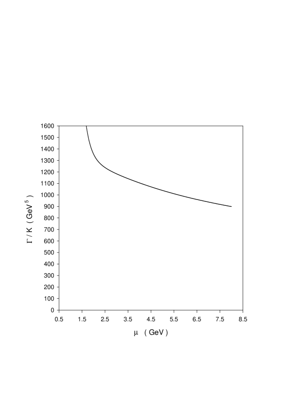
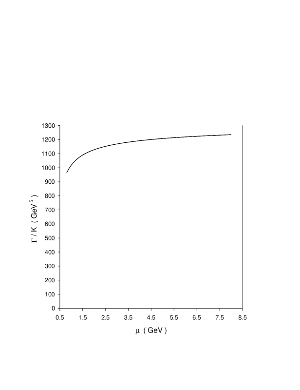
In Figure 1, we have plotted the mass- and scale-dependent portion of the rate (1),

ΓK=mb5F(mc2mb2)S[x(μ),L(μ)],(K192π3GF2|Vcb|2),\frac{\Gamma}{K}=m_{b}^{5}\,F\left(\frac{m_{c}^{2}}{m_{b}^{2}}\right)\,S\left[x(\mu),L(\mu)\right]\quad,\quad\left(K\equiv\frac{192\pi^{3}}{G_{F}^{2}\left|V_{cb}\right|^{2}}\right)~{}, (10)

as a function of μ𝜇\mu. The Fig. 1 curve is obtained by assuming mb=4.9GeVsubscript𝑚𝑏4.9GeVm_{b}=4.9\,{\rm GeV} [8], mc=0.3mbsubscript𝑚𝑐0.3subscript𝑚𝑏m_{c}=0.3m_{b} [2], and the central value b0=8.9subscript𝑏08.9b_{0}=-8.9 from the estimate [2] given in (5). Substantial scale dependence is evident from the figure: the rate increases monotonically with μ𝜇\mu, flattening out somewhat for larger values. Moreover the curve exhibits no PMS point (i.e., extremum), and at μ=mcmb=2.68GeV𝜇subscript𝑚𝑐subscript𝑚𝑏2.68GeV\mu=\sqrt{m_{c}m_{b}}=2.68\,{\rm GeV} yields a rate 10% smaller than the (still increasing) rate at μ=8GeV𝜇8GeV\mu=8\,{\rm GeV}, the flattest portion of the curve shown in the figure. Thus, the two-loop pole-mass calculation of the bcν¯𝑏𝑐superscriptsubscript¯𝜈b\to c\ell^{-}\bar{\nu}_{\ell} rate exhibits at best only poorly-controllable dependence on the choice of renormalization scale. Such scale dependence may compromise any subsequent “low-scale” mass expression devolving from the two-loop μ=mbmc𝜇subscript𝑚𝑏subscript𝑚𝑐\mu=\sqrt{m_{b}m_{c}} pole-mass rate.

Similar scale dependence and even worse apparent non-convergence characterise the two-loop order pole-mass calculation of the buν¯𝑏𝑢superscriptsubscript¯𝜈b\to u\ell^{-}\bar{\nu}_{\ell} rate, thereby motivating a recasting of the calculation in terms of the MS¯¯MS\overline{{\rm MS}} running b𝑏b-quark mass [3]. For four contributing flavours, the two-loop relationship between pole and MS¯¯MS\overline{{\rm MS}} running quark masses is [10]

mpole=m(μ)[1+(43+log(μ2m2(μ)))x(μ)+(10.3919+41572log(μ2m2(μ))+3724log2(μ2m2(μ)))x2(μ)]superscript𝑚𝑝𝑜𝑙𝑒𝑚𝜇delimited-[]143superscript𝜇2superscript𝑚2𝜇𝑥𝜇10.391941572superscript𝜇2superscript𝑚2𝜇3724superscript2superscript𝜇2superscript𝑚2𝜇superscript𝑥2𝜇m^{pole}=m(\mu)\left[1+\left(\frac{4}{3}+\log{\left(\frac{\mu^{2}}{m^{2}(\mu)}\right)}\right)x(\mu)+\left(10.3919+\frac{415}{72}\log{\left(\frac{\mu^{2}}{m^{2}(\mu)}\right)}+\frac{37}{24}\log^{2}{\left(\frac{\mu^{2}}{m^{2}(\mu)}\right)}\right)x^{2}(\mu)\right] (11)

By substituting this relation into (1), (4), and (5), we find that the fully MS¯¯MS\overline{{\rm MS}} version of the mass- and scale-dependent portion (10) of the bcν¯𝑏𝑐superscriptsubscript¯𝜈b\to c\ell^{-}\bar{\nu}_{\ell} decay rate (using the central value b0=8.9subscript𝑏08.9b_{0}=-8.9) is

ΓMS¯K=mb5(μ)F(mc2mb2){1+(5.00+5log(μ2mb2(μ)))x(μ)+[49.31.74log(μ2mc2(μ))+45.4log(μ2mb2(μ))+42524log2(μ2mb2(μ))]x2(μ)}.superscriptΓ¯𝑀𝑆𝐾superscriptsubscript𝑚𝑏5𝜇𝐹superscriptsubscript𝑚𝑐2superscriptsubscript𝑚𝑏215.005superscript𝜇2superscriptsubscript𝑚𝑏2𝜇𝑥𝜇delimited-[]49.31.74superscript𝜇2superscriptsubscript𝑚𝑐2𝜇45.4superscript𝜇2superscriptsubscript𝑚𝑏2𝜇42524superscript2superscript𝜇2superscriptsubscript𝑚𝑏2𝜇superscript𝑥2𝜇\begin{split}\frac{\Gamma^{\overline{MS}}}{K}=m_{b}^{5}(\mu)&\,F\left(\frac{m_{c}^{2}}{m_{b}^{2}}\right)\Biggl{\{}1+\left(5.00+5\log\left(\frac{\mu^{2}}{m_{b}^{2}(\mu)}\right)\right)x(\mu)\\ &+\left[49.3-1.74\,\log\left(\frac{\mu^{2}}{m_{c}^{2}(\mu)}\right)+45.4\,\log\left(\frac{\mu^{2}}{m_{b}^{2}(\mu)}\right)+\frac{425}{24}\,\log^{2}\left(\frac{\mu^{2}}{m_{b}^{2}(\mu)}\right)\right]x^{2}(\mu)\Biggr{\}}~{}.\end{split} (12)

Note that F(mc2/mb2)𝐹superscriptsubscript𝑚𝑐2superscriptsubscript𝑚𝑏2F\left(m_{c}^{2}/m_{b}^{2}\right) remains RG invariant if mcmc(μ)subscript𝑚𝑐subscript𝑚𝑐𝜇m_{c}\to m_{c}(\mu) and mbmb(μ)subscript𝑚𝑏subscript𝑚𝑏𝜇m_{b}\to m_{b}(\mu). If μ2=mb(μ)mc(μ)superscript𝜇2subscript𝑚𝑏𝜇subscript𝑚𝑐𝜇\mu^{2}=m_{b}(\mu)m_{c}(\mu) and if we continue to assume that mc(μ)=0.3mb(μ)subscript𝑚𝑐𝜇0.3subscript𝑚𝑏𝜇m_{c}(\mu)=0.3m_{b}(\mu), then

ΓMS¯K=mb5(μ)F(0.09)[11.02x(μ)+18.2x2(μ)],μ=0.3mb(μ)\frac{\Gamma^{\overline{MS}}}{K}=m_{b}^{5}(\mu)\,F\left(0.09\right)\left[1-1.02\,x\left(\mu\right)+18.2\,x^{2}\left(\mu\right)\right]\quad,\quad\mu=\sqrt{0.3}m_{b}(\mu) (13)

The convergence of this MS¯¯MS\overline{{\rm MS}} perturbative series is even more ill-behaved than its pole-mass version (3). Moreover, the scale dependence of (12) is shown in Figure 2 to be even more pronounced than that of the same rate in the pole-mass scheme (Figure 1)— Figure 2 displays a rate which decreases with μ𝜇\mu with no apparent PMS point.

Thus the MS¯¯MS\overline{{\rm MS}} approach, which substantially improves the perturbative series within the semileptonic bu𝑏𝑢b\to u rate [3], fails to improve the pole-mass expressions (13) for the semileptonic bc𝑏𝑐b\to c rate. If this latter rate is to be utilised to extract an estimate of |Vcb|subscript𝑉𝑐𝑏\left|V_{cb}\right| from the inclusive BXcν¯𝐵subscript𝑋𝑐superscriptsubscript¯𝜈B\to X_{c}\ell^{-}\bar{\nu}_{\ell} branching ratio, there is evident value in having an estimate of next-order corrections in order to obtain some control over renormalization-scale dependence. This three-loop order contribution to S[x(μ),L(μ)]𝑆𝑥𝜇𝐿𝜇S\left[x(\mu),L(\mu)\right] is necessarily of the form

ΔS3L[x(μ),L(μ)]=[c0+c1L(μ)+c2L2(μ)+c3L3(μ)]x3(μ)Δsuperscript𝑆3𝐿𝑥𝜇𝐿𝜇delimited-[]subscript𝑐0subscript𝑐1𝐿𝜇subscript𝑐2superscript𝐿2𝜇subscript𝑐3superscript𝐿3𝜇superscript𝑥3𝜇\Delta S^{3L}\left[x(\mu),L(\mu)\right]=\left[c_{0}+c_{1}L(\mu)+c_{2}L^{2}(\mu)+c_{3}L^{3}(\mu)\right]x^{3}(\mu) (14)

The RG equation (7) implies that

0=a1x+(b1a0β0)x2+(2b2β0a1)x2L+[c12β0b0a0β1]x3+[2c22β0b1β1a1]x3L+[3c32β0b2]x3L2+𝒪(x4).0subscript𝑎1𝑥subscript𝑏1subscript𝑎0subscript𝛽0superscript𝑥22subscript𝑏2subscript𝛽0subscript𝑎1superscript𝑥2𝐿delimited-[]subscript𝑐12subscript𝛽0subscript𝑏0subscript𝑎0subscript𝛽1superscript𝑥3delimited-[]2subscript𝑐22subscript𝛽0subscript𝑏1subscript𝛽1subscript𝑎1superscript𝑥3𝐿delimited-[]3subscript𝑐32subscript𝛽0subscript𝑏2superscript𝑥3superscript𝐿2𝒪superscript𝑥4\begin{split}0=&a_{1}x+\left(b_{1}-a_{0}\beta_{0}\right)x^{2}+\left(2b_{2}-\beta_{0}a_{1}\right)x^{2}L+\left[c_{1}-2\beta_{0}b_{0}-a_{0}\beta_{1}\right]x^{3}+\left[2c_{2}-2\beta_{0}b_{1}-\beta_{1}a_{1}\right]x^{3}L\\ &+\left[3c_{3}-2\beta_{0}b_{2}\right]x^{3}L^{2}+{\cal O}\left(x^{4}\right)~{}.\end{split} (15)

The set of results (9) are evident from the requirement that 𝒪(x)𝒪𝑥{\cal O}(x), 𝒪(x2)𝒪superscript𝑥2{\cal O}\left(x^{2}\right) and 𝒪(x2L)𝒪superscript𝑥2𝐿{\cal O}\left(x^{2}L\right) terms in (15) separately vanish. The vanishing of subsequent terms in (15) implies that

c1=2b0β0+a0β1,c2=a0β02,c3=0.formulae-sequencesubscript𝑐12subscript𝑏0subscript𝛽0subscript𝑎0subscript𝛽1formulae-sequencesubscript𝑐2subscript𝑎0superscriptsubscript𝛽02subscript𝑐30c_{1}=2b_{0}\beta_{0}+a_{0}\beta_{1}~{},~{}c_{2}=a_{0}\beta_{0}^{2}~{},~{}c_{3}=0~{}. (16)

For a0subscript𝑎0a_{0} and b0subscript𝑏0b_{0} as given in (5) and three massless flavours (as appropriate to phenomenology devolving from αs(mτ)subscript𝛼𝑠subscript𝑚𝜏\alpha_{s}\left(m_{\tau}\right) [6]),

c1=42.4±1.3,c2=7.25,c3=0.formulae-sequencesubscript𝑐1plus-or-minus42.41.3formulae-sequencesubscript𝑐27.25subscript𝑐30c_{1}=-42.4\pm 1.3~{},~{}c_{2}=-7.25~{},~{}c_{3}=0~{}. (17)

The coefficient c0subscript𝑐0c_{0}, however, is RG-inaccessible to these orders of perturbation theory, and requires a direct three-loop calculation. In the absence of such a calculation, we estimate c0subscript𝑐0c_{0} in the section which follows via asymptotic Padé approximant methodology, in much the same way as in a prior estimate [13] of the three-loop contribution to the buν¯𝑏𝑢superscriptsubscript¯𝜈b\to u\ell^{-}\bar{\nu}_{\ell} decay rate.

3 RG/Padé Estimate of c0subscript𝑐0c_{0}

Consider a perturbative field-theoretical series with N+M𝑁𝑀N+M known terms:

S(x)=1+R1x+R2x2++RN+MxN+M+.𝑆𝑥1subscript𝑅1𝑥subscript𝑅2superscript𝑥2subscript𝑅𝑁𝑀superscript𝑥𝑁𝑀S(x)=1+R_{1}x+R_{2}x^{2}+\ldots+R_{N+M}x^{N+M}+\ldots~{}~{}. (18)

The set of known coefficients {R1,R2,,RN+M}subscript𝑅1subscript𝑅2subscript𝑅𝑁𝑀\{R_{1},R_{2},\ldots,R_{N+M}\} is sufficient to determine in full the N+M𝑁𝑀N+M coefficients characterising an [N|M]delimited-[]conditional𝑁𝑀[N|M] Padé-approximant to the series S𝑆S:

S[N|M](x)1+a1x+a2x2++aNxN1+b1x+b2x2++bMxM.subscript𝑆delimited-[]conditional𝑁𝑀𝑥1subscript𝑎1𝑥subscript𝑎2superscript𝑥2subscript𝑎𝑁superscript𝑥𝑁1subscript𝑏1𝑥subscript𝑏2superscript𝑥2subscript𝑏𝑀superscript𝑥𝑀S_{[N|M]}(x)\equiv\frac{1+a_{1}x+a_{2}x^{2}+\ldots+a_{N}x^{N}}{1+b_{1}x+b_{2}x^{2}+\ldots+b_{M}x^{M}}~{}. (19)

The coefficients {a1,,aN,b1,,bM}subscript𝑎1subscript𝑎𝑁subscript𝑏1subscript𝑏𝑀\{a_{1},\ldots,a_{N},b_{1},\ldots,b_{M}\} are obtained by the requirement that the power-series expansion of S[N|M](x)subscript𝑆delimited-[]conditional𝑁𝑀𝑥S_{[N|M]}(x) recovers the N+M𝑁𝑀N+M known coefficients within (18), the series S(x)𝑆𝑥S(x). The next 𝒪(xN+M+1)𝒪superscript𝑥𝑁𝑀1{\cal O}\left(x^{N+M+1}\right) term in this power series is a Padé approximant prediction for the first unknown coefficient RN+M+1subscript𝑅𝑁𝑀1R_{N+M+1}. For example, if only the next-to-leading order coefficient R1subscript𝑅1R_{1} is known, one can use this coefficient to construct a [0|1]delimited-[]conditional01[0|1] approximant to the series (18),

S[0|1](x)=11R1x=1+R1x+R12x2+,subscript𝑆delimited-[]conditional01𝑥11subscript𝑅1𝑥1subscript𝑅1𝑥superscriptsubscript𝑅12superscript𝑥2S_{[0|1]}(x)=\frac{1}{1-R_{1}x}=1+R_{1}x+R_{1}^{2}x^{2}+\ldots~{}, (20)

for which R12superscriptsubscript𝑅12R_{1}^{2} is the predicted value of R2subscript𝑅2R_{2}:

R2[0|1]=R12.superscriptsubscript𝑅2delimited-[]conditional01superscriptsubscript𝑅12R_{2}^{[0|1]}=R_{1}^{2}~{}. (21)

Similarly, if R1subscript𝑅1R_{1} and R2subscript𝑅2R_{2} are known (corresponding to two subleading orders of perturbation theory), one has enough information to construct a [1|1]delimited-[]conditional11[1|1] approximant to the series (18):

S[1|1](x)=1+(R12R2R1)x1R2R1x=1+R1x+R2x2+R22R1x3+.subscript𝑆delimited-[]conditional11𝑥1superscriptsubscript𝑅12subscript𝑅2subscript𝑅1𝑥1subscript𝑅2subscript𝑅1𝑥1subscript𝑅1𝑥subscript𝑅2superscript𝑥2superscriptsubscript𝑅22subscript𝑅1superscript𝑥3S_{[1|1]}(x)=\frac{1+\left(\frac{R_{1}^{2}-R_{2}}{R_{1}}\right)x}{1-\frac{R_{2}}{R_{1}}x}=1+R_{1}x+R_{2}x^{2}+\frac{R_{2}^{2}}{R_{1}}x^{3}+\ldots~{}. (22)

The predicted value for the unknown coefficient R3subscript𝑅3R_{3} is

R3[1|1]=R22/R1superscriptsubscript𝑅3delimited-[]conditional11superscriptsubscript𝑅22subscript𝑅1R_{3}^{[1|1]}=R_{2}^{2}/R_{1} (23)

In general, one can always use an [N|M]delimited-[]conditional𝑁𝑀[N|M] approximant (19) to predict the first unknown series coefficient RN+M+1subscript𝑅𝑁𝑀1R_{N+M+1}. Such predictions have accuracy which increases as N𝑁N and M𝑀M increase. For perturbative field-theoretical series (characterised by asymptotic RNN!similar-tosubscript𝑅𝑁𝑁R_{N}\sim N! behaviour) the accuracy of such predictions has been argued by Ellis, Karliner and Samuel to satisfy the relative error formula [14]

ΔRN+M+1[N|M]RN+M+1true=RN+M+1[N|M]RN+M+1trueRN+M+1true=M!AM(N+M+aM+b)MΔsuperscriptsubscript𝑅𝑁𝑀1delimited-[]conditional𝑁𝑀subscriptsuperscript𝑅𝑡𝑟𝑢𝑒𝑁𝑀1superscriptsubscript𝑅𝑁𝑀1delimited-[]conditional𝑁𝑀superscriptsubscript𝑅𝑁𝑀1𝑡𝑟𝑢𝑒subscriptsuperscript𝑅𝑡𝑟𝑢𝑒𝑁𝑀1𝑀superscript𝐴𝑀superscript𝑁𝑀𝑎𝑀𝑏𝑀\frac{\Delta R_{N+M+1}^{[N|M]}}{R^{true}_{N+M+1}}=\frac{R_{N+M+1}^{[N|M]}-R_{N+M+1}^{true}}{R^{true}_{N+M+1}}=-\frac{M!A^{M}}{\left(N+M+aM+b\right)^{M}} (24)

where A𝐴A, a𝑎a, and b𝑏b are constants to be determined. Of particular interest are the relative errors obtained from (24) for the predictions (21) and (23)

R12R2R2=A1+(a+b),superscriptsubscript𝑅12subscript𝑅2subscript𝑅2𝐴1𝑎𝑏\displaystyle\frac{R_{1}^{2}-R_{2}}{R_{2}}=-\frac{A}{1+(a+b)}~{}, (25)
R22R1R3R3=A2+(a+b).superscriptsubscript𝑅22subscript𝑅1subscript𝑅3subscript𝑅3𝐴2𝑎𝑏\displaystyle\frac{\frac{R_{2}^{2}}{R_{1}}-R_{3}}{R_{3}}=-\frac{A}{2+(a+b)}~{}. (26)

Denoting the constant a+b=k𝑎𝑏𝑘a+b=k, we can eliminate the other constant A𝐴A within (25,26) and solve for R3subscript𝑅3R_{3} algebraically to obtain the improved estimate

R3=(2+k)R23(1+k)R13+R1R2.subscript𝑅32𝑘superscriptsubscript𝑅231𝑘superscriptsubscript𝑅13subscript𝑅1subscript𝑅2R_{3}=\frac{(2+k)R_{2}^{3}}{(1+k)R_{1}^{3}+R_{1}R_{2}}~{}. (27)

The assumption k=0𝑘0k=0 has been utilised in prior applications to predict successfully the third subleading contribution to the QCD MS¯¯MS\overline{{\rm MS}} β𝛽\beta-function [14], the DRED SQCD β𝛽\beta-function [15], the MS¯¯MS\overline{{\rm MS}} β𝛽\beta-function for massive scalar field theory [16], as well as to obtain estimates of such contributions for a number of processes calculated in the MS¯¯MS\overline{{\rm MS}} scheme: SM [17] and MSSM [18] Higgs \to 2 gluon decay rates, buν¯𝑏𝑢superscriptsubscript¯𝜈b\to u\ell^{-}\bar{\nu}_{\ell} [13], W+WZZsuperscript𝑊superscript𝑊𝑍𝑍W^{+}W^{-}\to ZZ [16], and the QCD static potential function [19].

The choice k=0𝑘0k=0, however, is ill-suited to pole-mass calculations. To see this, consider the series (4, 14) within (1) characterising the pole-mass expression for the bcν¯𝑏𝑐superscriptsubscript¯𝜈b\to c\ell^{-}\bar{\nu}_{\ell} decay rate

S[x,L]=1+(a0+a1L)x+(b0+b1L+b2L2)x2+(c0+c1L+c2L2+c3L3)x3𝑆𝑥𝐿1subscript𝑎0subscript𝑎1𝐿𝑥subscript𝑏0subscript𝑏1𝐿subscript𝑏2superscript𝐿2superscript𝑥2subscript𝑐0subscript𝑐1𝐿subscript𝑐2superscript𝐿2subscript𝑐3superscript𝐿3superscript𝑥3\displaystyle S[x,L]=1+\left(a_{0}+a_{1}L\right)x+\left(b_{0}+b_{1}L+b_{2}L^{2}\right)x^{2}+\left(c_{0}+c_{1}L+c_{2}L^{2}+c_{3}L^{3}\right)x^{3} (28)
x=αs(μ)π,L=log(μ2mbmc)\displaystyle x=\frac{\alpha_{s}(\mu)}{\pi}\quad,\quad L=\log\left(\frac{\mu^{2}}{m_{b}m_{c}}\right)

We have already seen that a0=1.67subscript𝑎01.67a_{0}=-1.67, a1=0subscript𝑎10a_{1}=0, b08.9±0.3subscript𝑏0plus-or-minus8.90.3b_{0}\cong-8.9\pm 0.3, b1=a0β0=3.48subscript𝑏1subscript𝑎0subscript𝛽03.48b_{1}=a_{0}\beta_{0}=-3.48, b2=0subscript𝑏20b_{2}=0. The above series is in the form of (18) with R1subscript𝑅1R_{1} and R2subscript𝑅2R_{2} respectively identified with a0+a1Lsubscript𝑎0subscript𝑎1𝐿a_{0}+a_{1}L and b0+b1L+b2L2subscript𝑏0subscript𝑏1𝐿subscript𝑏2superscript𝐿2b_{0}+b_{1}L+b_{2}L^{2}. If k=0𝑘0k=0, we see from (27) that

R3=2(b0+b1L)3a0(a02+b0+b1L)=2b12a0L2+2b1a0(2b0a02)L+𝒪(L0)subscript𝑅32superscriptsubscript𝑏0subscript𝑏1𝐿3subscript𝑎0superscriptsubscript𝑎02subscript𝑏0subscript𝑏1𝐿2superscriptsubscript𝑏12subscript𝑎0superscript𝐿22subscript𝑏1subscript𝑎02subscript𝑏0superscriptsubscript𝑎02𝐿𝒪superscript𝐿0R_{3}=\frac{2\left(b_{0}+b_{1}L\right)^{3}}{a_{0}\left(a_{0}^{2}+b_{0}+b_{1}L\right)}=\frac{2b_{1}^{2}}{a_{0}}L^{2}+\frac{2b_{1}}{a_{0}}\left(2b_{0}-a_{0}^{2}\right)L+{\cal O}\left(L^{0}\right) (29)

Comparing this expression to the form (14) anticipated for the third subleading order of S[x,L]𝑆𝑥𝐿S[x,L], we necessarily obtain the following predictions for the RG accessible coefficients c2subscript𝑐2c_{2}, c1subscript𝑐1c_{1}:

c2=2b12a0=2a0β02,subscript𝑐22superscriptsubscript𝑏12subscript𝑎02subscript𝑎0superscriptsubscript𝛽02\displaystyle c_{2}=2\frac{b_{1}^{2}}{a_{0}}=2a_{0}\beta_{0}^{2}~{}, (30)
c1=2(2b0a02)b1a0=4β0b02β0a02subscript𝑐122subscript𝑏0superscriptsubscript𝑎02subscript𝑏1subscript𝑎04subscript𝛽0subscript𝑏02subscript𝛽0superscriptsubscript𝑎02\displaystyle c_{1}=2\left(2b_{0}-a_{0}^{2}\right)\frac{b_{1}}{a_{0}}=4\beta_{0}b_{0}-2\beta_{0}a_{0}^{2} (31)

It is evident from (16,17) that these predictions are quite poor; (30) is double the true value for c2subscript𝑐2c_{2}, as obtained in (17), and c1subscript𝑐1c_{1} is also badly overestimated [for values (9) and the central value b0=8.9subscript𝑏08.9b_{0}=-8.9, eq. (31) implies that c1=85.8subscript𝑐185.8c_{1}=-85.8, in contrast to the correct (RG) value c1=42.4subscript𝑐142.4c_{1}=-42.4].

For a given choice of k𝑘k, estimates of the coefficients cisubscript𝑐𝑖c_{i} characterising the third subleading order have been obtained for correlation functions [20] and the buν¯𝑏𝑢superscriptsubscript¯𝜈b\to u\ell^{-}\bar{\nu}_{\ell} rate [13] by moments of R3subscript𝑅3R_{3}, as estimated in (27), over the entire ultraviolet region (e.g., μ2/(mbmc)1superscript𝜇2subscript𝑚𝑏subscript𝑚𝑐1\mu^{2}/(m_{b}m_{c})\geq 1 for the case at hand). These moments are then equated to corresponding moments of R3=c0+c1L+c2L2+c3L3subscript𝑅3subscript𝑐0subscript𝑐1𝐿subscript𝑐2superscript𝐿2subscript𝑐3superscript𝐿3R_{3}=c_{0}+c_{1}L+c_{2}L^{2}+c_{3}L^{3} in order to obtain values for {c0,c1,c2,c3}subscript𝑐0subscript𝑐1subscript𝑐2subscript𝑐3\{c_{0},c_{1},c_{2},c_{3}\}. If we define w=mbmc/μ2𝑤subscript𝑚𝑏subscript𝑚𝑐superscript𝜇2w=m_{b}m_{c}/\mu^{2} (L=logw𝐿𝑤L=-\log w), the moments

Nj=(j+2)01wj+1R3(w)dwsubscript𝑁𝑗𝑗2superscriptsubscript01superscript𝑤𝑗1subscript𝑅3𝑤differential-d𝑤N_{j}=(j+2)\int\limits_{0}^{1}w^{j+1}R_{3}(w)\mathrm{d}w (32)

can be obtained using (27) for the integrand R3subscript𝑅3R_{3}, which becomes a function of w𝑤w for our pole mass case by virtue of the w𝑤w-dependence of R2subscript𝑅2R_{2}: R1=a0subscript𝑅1subscript𝑎0R_{1}=a_{0}, R2=b0b1logwsubscript𝑅2subscript𝑏0subscript𝑏1𝑤R_{2}=b_{0}-b_{1}\log w. After (numerical) computation of the values of Njsubscript𝑁𝑗N_{j}, the coefficients cisubscript𝑐𝑖c_{i} are obtained by equating such values to the corresponding integrals

Nj=(j+2)01wj+1(c0c1logw+c2log2wc3log3w)dw.subscript𝑁𝑗𝑗2superscriptsubscript01superscript𝑤𝑗1subscript𝑐0subscript𝑐1𝑤subscript𝑐2superscript2𝑤subscript𝑐3superscript3𝑤differential-d𝑤N_{j}=(j+2)\int\limits_{0}^{1}w^{j+1}\left(c_{0}-c_{1}\log w+c_{2}\log^{2}w-c_{3}\log^{3}w\right)\mathrm{d}w~{}. (33)

In particular, we see that

N1=c0+c1+2c2+6c3subscript𝑁1subscript𝑐0subscript𝑐12subscript𝑐26subscript𝑐3\displaystyle N_{-1}=c_{0}+c_{1}+2c_{2}+6c_{3} (34)
N0=c0+12c1+12c2+34c3subscript𝑁0subscript𝑐012subscript𝑐112subscript𝑐234subscript𝑐3\displaystyle N_{0}=c_{0}+\frac{1}{2}c_{1}+\frac{1}{2}c_{2}+\frac{3}{4}c_{3} (35)
N1=c0+13c1+29c2+29c3subscript𝑁1subscript𝑐013subscript𝑐129subscript𝑐229subscript𝑐3\displaystyle N_{1}=c_{0}+\frac{1}{3}c_{1}+\frac{2}{9}c_{2}+\frac{2}{9}c_{3} (36)
N2=c0+14c1+18c2+332c3.subscript𝑁2subscript𝑐014subscript𝑐118subscript𝑐2332subscript𝑐3\displaystyle N_{2}=c_{0}+\frac{1}{4}c_{1}+\frac{1}{8}c_{2}+\frac{3}{32}c_{3}~{}. (37)

If k1𝑘1k\neq-1, such a procedure is seen to lead to a non-zero value of c3subscript𝑐3c_{3}, in contradiction to the result c3=0subscript𝑐30c_{3}=0 (16) necessarily following from application of the RG equation (7) within the pole mass scheme. For the case k=1𝑘1k=-1, however, the result (27) collapses to the naive estimate (23), which in the pole mass scheme is necessarily a degree-2 polynomial in L𝐿L:

R3(k=1)=R22R1=1a0(b0+b1L)2=b12a0L2+2b1b0a0L+b02a0superscriptsubscript𝑅3𝑘1superscriptsubscript𝑅22subscript𝑅11subscript𝑎0superscriptsubscript𝑏0subscript𝑏1𝐿2superscriptsubscript𝑏12subscript𝑎0superscript𝐿22subscript𝑏1subscript𝑏0subscript𝑎0𝐿superscriptsubscript𝑏02subscript𝑎0R_{3}^{(k=-1)}=\frac{R_{2}^{2}}{R_{1}}=\frac{1}{a_{0}}\left(b_{0}+b_{1}L\right)^{2}=\frac{b_{1}^{2}}{a_{0}}L^{2}+2\frac{b_{1}b_{0}}{a_{0}}L+\frac{b_{0}^{2}}{a_{0}} (38)

The moment procedure described above then reduces to fitting the degree-3 polynomial R3=c3L3+c2L2+c1L+c0subscript𝑅3subscript𝑐3superscript𝐿3subscript𝑐2superscript𝐿2subscript𝑐1𝐿subscript𝑐0R_{3}=c_{3}L^{3}+c_{2}L^{2}+c_{1}L+c_{0} to the degree-2 polynomial in (38). Such a fit necessarily reduces to equating the powers of L𝐿L in these two expressions. We thus find that c3subscript𝑐3c_{3} must be zero, and that

c2=b12a0=a0β02subscript𝑐2superscriptsubscript𝑏12subscript𝑎0subscript𝑎0superscriptsubscript𝛽02\displaystyle c_{2}=\frac{b_{1}^{2}}{a_{0}}=a_{0}\beta_{0}^{2} (39)
c1=2b1b0a0=2β0b0subscript𝑐12subscript𝑏1subscript𝑏0subscript𝑎02subscript𝛽0subscript𝑏0\displaystyle c_{1}=2\frac{b_{1}b_{0}}{a_{0}}=2\beta_{0}b_{0} (40)
c0=b02a0subscript𝑐0superscriptsubscript𝑏02subscript𝑎0\displaystyle c_{0}=\frac{b_{0}^{2}}{a_{0}} (41)

Equation (39) is in exact agreement with the result (16) obtained via RG-invariance from (7). Equation (40) represents the first (and dominant) contribution to the RG-determination of c1subscript𝑐1c_{1} in (16). For the central value b0=8.9subscript𝑏08.9b_{0}=-8.9 (and nf=4subscript𝑛𝑓4n_{f}=4) the (40) prediction c1=37.1subscript𝑐137.1c_{1}=-37.1 is not far from the true value c1=42.4subscript𝑐142.4c_{1}=-42.4. The accuracy of these results provide some support to the naive estimate c0=47.4subscript𝑐047.4c_{0}=-47.4 obtained via (41) for the RG-inaccessible coefficient c0subscript𝑐0c_{0}.

We can further improve our estimate for c0subscript𝑐0c_{0} by finding the value of k𝑘k within (27) which, when used within the integrand of (32) to match the moments Njsubscript𝑁𝑗N_{j} to (3437), most closely reproduces the true values of c2subscript𝑐2c_{2} and c1subscript𝑐1c_{1} , as determined by RG methods in (16) and (17). In such a procedure we obtain estimated values for c3subscript𝑐3c_{3}, c2subscript𝑐2c_{2}, c1subscript𝑐1c_{1}, and c0subscript𝑐0c_{0} that depend explicitly on k𝑘k:

c0(k)=16N1(k)+4N0(k)272N1(k)+323N2(k)subscript𝑐0𝑘16subscript𝑁1𝑘4subscript𝑁0𝑘272subscript𝑁1𝑘323subscript𝑁2𝑘\displaystyle c_{0}(k)=-\frac{1}{6}N_{-1}(k)+4N_{0}(k)-\frac{27}{2}N_{1}(k)+\frac{32}{3}N_{2}(k) (42)
c1(k)=32N1(k)32N0(k)+1892N1(k)64N2(k)subscript𝑐1𝑘32subscript𝑁1𝑘32subscript𝑁0𝑘1892subscript𝑁1𝑘64subscript𝑁2𝑘\displaystyle c_{1}(k)=\frac{3}{2}N_{-1}(k)-32N_{0}(k)+\frac{189}{2}N_{1}(k)-64N_{2}(k) (43)
c2(k)=136N1(k)+38N0(k)1892N1(k)+1763N2(k)subscript𝑐2𝑘136subscript𝑁1𝑘38subscript𝑁0𝑘1892subscript𝑁1𝑘1763subscript𝑁2𝑘\displaystyle c_{2}(k)=-\frac{13}{6}N_{-1}(k)+38N_{0}(k)-\frac{189}{2}N_{1}(k)+\frac{176}{3}N_{2}(k) (44)
c3(k)=23N1(k)8N0(k)+18N1(k)323N2(k)subscript𝑐3𝑘23subscript𝑁1𝑘8subscript𝑁0𝑘18subscript𝑁1𝑘323subscript𝑁2𝑘\displaystyle c_{3}(k)=\frac{2}{3}N_{-1}(k)-8N_{0}(k)+18N_{1}(k)-\frac{32}{3}N_{2}(k) (45)

where

Nj(k)=(j+2)01wj+1[(2+k)(b0b1logw)3(1+k)a03+a0(b0b1logw)]dwsubscript𝑁𝑗𝑘𝑗2superscriptsubscript01superscript𝑤𝑗1delimited-[]2𝑘superscriptsubscript𝑏0subscript𝑏1𝑤31𝑘superscriptsubscript𝑎03subscript𝑎0subscript𝑏0subscript𝑏1𝑤differential-d𝑤N_{j}(k)=(j+2)\int\limits_{0}^{1}w^{j+1}\left[\frac{(2+k)\left(b_{0}-b_{1}\log w\right)^{3}}{(1+k)a_{0}^{3}+a_{0}\left(b_{0}-b_{1}\log w\right)}\right]\,\mathrm{d}w (46)

We then use the explicit values for c1subscript𝑐1c_{1} and c2subscript𝑐2c_{2} obtained from (17) by RG methods to optimize the sum of the squares of the relative error of estimated values of c1subscript𝑐1c_{1} and c2subscript𝑐2c_{2},

Δ(k)=(c2(k)a0β02a0β02)2+(c1(k)(2β0b0a0β1)2β0b0a0β1)2Δ𝑘superscriptsubscript𝑐2𝑘subscript𝑎0superscriptsubscript𝛽02subscript𝑎0superscriptsubscript𝛽022superscriptsubscript𝑐1𝑘2subscript𝛽0subscript𝑏0subscript𝑎0subscript𝛽12subscript𝛽0subscript𝑏0subscript𝑎0subscript𝛽12\Delta(k)=\left(\frac{c_{2}(k)-a_{0}\beta_{0}^{2}}{a_{0}\beta_{0}^{2}}\right)^{2}+\left(\frac{c_{1}(k)-\left(2\beta_{0}b_{0}-a_{0}\beta_{1}\right)}{2\beta_{0}b_{0}-a_{0}\beta_{1}}\right)^{2} (47)

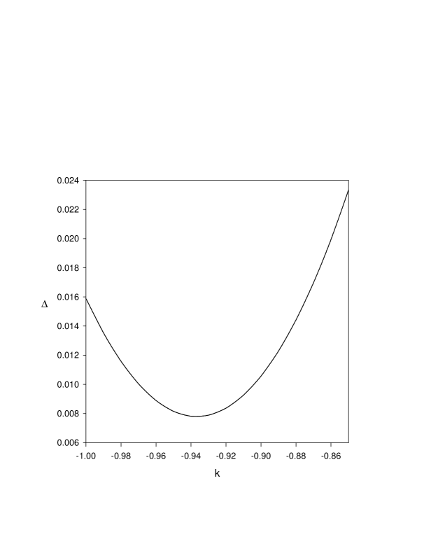
with respect to k𝑘k. For the set of values a0=1.67subscript𝑎01.67a_{0}=-1.67, b0=8.9subscript𝑏08.9b_{0}=-8.9, β0=25/12subscript𝛽02512\beta_{0}=25/12, β1=77/24subscript𝛽17724\beta_{1}=77/24, we find a clear minimum of Δ(k)Δ𝑘\Delta(k) at k=0.94𝑘0.94k=-0.94, as evident from Figure 3, consistent with the case made in the preceding paragraph for an optimal k𝑘k value close to k=1𝑘1k=-1. Corresponding k=0.94𝑘0.94k=-0.94 values for the moments Njsubscript𝑁𝑗N_{j} are obtained numerically via (46)

N1=106.3,N0=74.92,N1=66.17,N2=62.12formulae-sequencesubscript𝑁1106.3formulae-sequencesubscript𝑁074.92formulae-sequencesubscript𝑁166.17subscript𝑁262.12N_{-1}=-106.3~{},~{}N_{0}=-74.92~{},~{}N_{1}=-66.17~{},~{}N_{2}=-62.12 (48)

and these values lead via (42)–(45)to the following estimates for the third subleading order coefficients:

c3=2.0×10⁴,c2=7.68,c1=39.7,c0=51.2formulae-sequencesubscript𝑐32.0superscript104formulae-sequencesubscript𝑐27.68formulae-sequencesubscript𝑐139.7subscript𝑐051.2c_{3}=2.0\times 10^{-4}~{},~{}c_{2}=-7.68~{},~{}c_{1}=-39.7~{},~{}c_{0}=-51.2 (49)

These values reflect excellent agreement with the RG values (17). The above estimate for the RG-inaccessible coefficient c0subscript𝑐0c_{0} is only 20% larger in magnitude than the naive prediction (41), indicative of the internal consistency of the methodology.

We conclude by noting that four separate estimates of c0subscript𝑐0c_{0} can be obtained from (34)–(37) by substituting into these equations the optimal Njsubscript𝑁𝑗N_{j} values (48) as well as the true values c3=0subscript𝑐30c_{3}=0, c1=42.4subscript𝑐142.4c_{1}=-42.4 and c2=7.25subscript𝑐27.25c_{2}=-7.25 as determined by RG invariance (17) in the previous section. Solving each equation separately for c0subscript𝑐0c_{0}, we find that

c0=N1c12c26c3=49.4,subscript𝑐0subscript𝑁1subscript𝑐12subscript𝑐26subscript𝑐349.4\displaystyle c_{0}=N_{-1}-c_{1}-2c_{2}-6c_{3}=-49.4~{}, (50)
c0=N012c112c234c3=50.1,subscript𝑐0subscript𝑁012subscript𝑐112subscript𝑐234subscript𝑐350.1\displaystyle c_{0}=N_{0}-\frac{1}{2}c_{1}-\frac{1}{2}c_{2}-\frac{3}{4}c_{3}=-50.1~{}, (51)
c0=N113c129c229c3=50.4,subscript𝑐0subscript𝑁113subscript𝑐129subscript𝑐229subscript𝑐350.4\displaystyle c_{0}=N_{1}-\frac{1}{3}c_{1}-\frac{2}{9}c_{2}-\frac{2}{9}c_{3}=-50.4~{}, (52)
c0=N214c118c2332c3=50.6.subscript𝑐0subscript𝑁214subscript𝑐118subscript𝑐2332subscript𝑐350.6\displaystyle c_{0}=N_{2}-\frac{1}{4}c_{1}-\frac{1}{8}c_{2}-\frac{3}{32}c_{3}=-50.6~{}. (53)

The estimates (50)–(53) are remarkably consistent with each other and only slightly smaller in magnitude than the estimate in (49) obtained without RG inputs for {c1,c2,c3}subscript𝑐1subscript𝑐2subscript𝑐3\{c_{1},~{}c_{2}~{},c_{3}\}.

In estimating the third subleading order of (14), the series within the rate (1), we choose (51) as the most central of our c0subscript𝑐0c_{0} estimates, in conjunction with the explicit RG determinations of c1subscript𝑐1c_{1} and c2subscript𝑐2c_{2} (c3=0subscript𝑐30c_{3}=0). This set of values is obtained, as noted earlier, for the central value estimate [2] of b0subscript𝑏0b_{0}:

b0=8.9:{c0,c1,c2}{50.1,42.4,7.25}.:subscript𝑏08.9subscript𝑐0subscript𝑐1subscript𝑐250.142.47.25b_{0}=-8.9~{}:~{}\{c_{0},c_{1},c_{2}\}\cong\{-50.1,-42.4,-7.25\}~{}. (54)

Precisely the same procedure can be used to obtain corresponding estimates of {c0,c1,c2}subscript𝑐0subscript𝑐1subscript𝑐2\{c_{0},c_{1},c_{2}\} for the extremes of the b0=8.9±0.3subscript𝑏0plus-or-minus8.90.3b_{0}=-8.9\pm 0.3 range obtained in [2] (see footnote 1):

b0=9.2:{c0,c1,c2}{53.6,43.7,7.25}:subscript𝑏09.2subscript𝑐0subscript𝑐1subscript𝑐253.643.77.25\displaystyle b_{0}=-9.2~{}:~{}\{c_{0},c_{1},c_{2}\}\cong\{-53.6,-43.7,-7.25\} (55)
b0=8.6:{c0,c1,c2}{47.5,41.2,7.25}.:subscript𝑏08.6subscript𝑐0subscript𝑐1subscript𝑐247.541.27.25\displaystyle b_{0}=-8.6~{}:~{}\{c_{0},c_{1},c_{2}\}\cong\{-47.5,-41.2,-7.25\}~{}. (56)

These estimates are obtained in precisely the same way as those of (54): c1subscript𝑐1c_{1} and c2subscript𝑐2c_{2} are identified with their RG values via (17), and c0subscript𝑐0c_{0} is determined via (51) with N0(k)subscript𝑁0𝑘N_{0}(k) [see Eq. (46)] evaluated at a value of k𝑘k which minimizes Δ(k)Δ𝑘\Delta(k) [see Eq. (47)]. The coefficient c3=0subscript𝑐30c_{3}=0 for all cases, as evident in the previous section from RG-invariance. For the b0=9.2subscript𝑏09.2b_{0}=-9.2 case, the minimizing value k=0.94𝑘0.94k=-0.94 is the same as for b0=8.9subscript𝑏08.9b_{0}=-8.9. For b0=8.6subscript𝑏08.6b_{0}=-8.6, the minimum value of Δ(k)Δ𝑘\Delta(k) is found to occur when k=0.93𝑘0.93k=-0.93.

4 Scale Dependence of the Three-Loop Rate

If b0=8.9subscript𝑏08.9b_{0}=-8.9, the three-loop bcν¯𝑏𝑐superscriptsubscript¯𝜈b\to c\ell^{-}\bar{\nu}_{\ell} inclusive estimated rate is given by (1) with

S[x(μ),L(μ)]=11.67x+(8.93.479L)x2+(50.142.4L7.25L2)x3.𝑆𝑥𝜇𝐿𝜇11.67𝑥8.93.479𝐿superscript𝑥250.142.4𝐿7.25superscript𝐿2superscript𝑥3S\left[x(\mu),L(\mu)\right]=1-1.67x+\left(-8.9-3.479L\right)x^{2}+\left(-50.1-42.4L-7.25L^{2}\right)x^{3}~{}. (57)

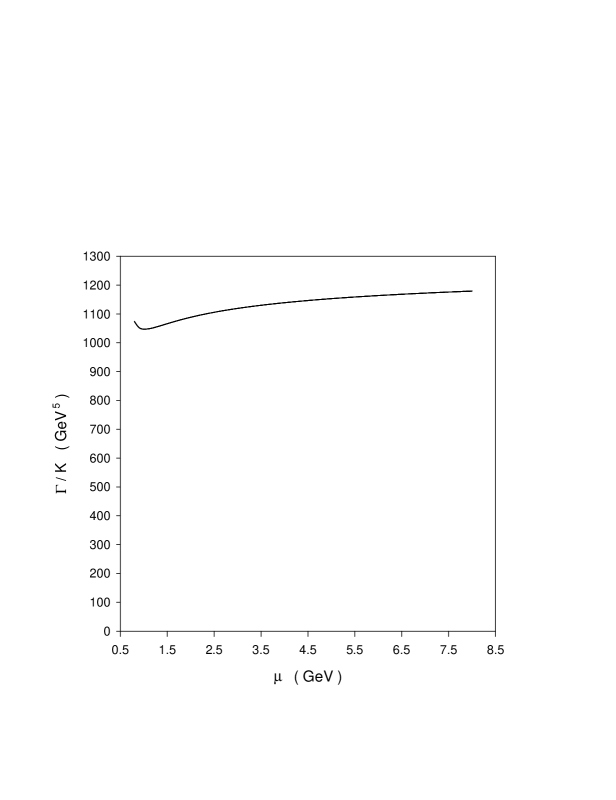
The coefficients of x3superscript𝑥3x^{3} are those of (54), as estimated in the previous section. Figure 4 displays a plot of the μ𝜇\mu- (scale-) dependence of the “reduced” three-loop rate (10) with S[x,L]𝑆𝑥𝐿S[x,L] given by (57). The pole masses mbsubscript𝑚𝑏m_{b} and mcsubscript𝑚𝑐m_{c} are assumed to be mb=4.9GeVsubscript𝑚𝑏4.9GeVm_{b}=4.9\,{\rm GeV} and mc=0.3mb=1.47GeVsubscript𝑚𝑐0.3subscript𝑚𝑏1.47GeVm_{c}=0.3m_{b}=1.47\,{\rm GeV} consistent with values used in [2]. Figure 4 clearly displays a much flatter μ𝜇\mu-dependence than the two-loop rate plotted in Fig. 1. In addition to this diminished dependence on the renormalization scale μ𝜇\mu, the rate plotted in Fig. 4 also exhibits a distinct minimum at μ=1.0GeV𝜇1.0GeV\mu=1.0\,{\rm GeV}. At this PMS (minimal-sensitivity) value of μ𝜇\mu, the successive terms of the series S[x,L]𝑆𝑥𝐿S[x,L] exhibit reasonable convergence:

S[x(1.0GeV),L(1.0GeV)]=10.2580.049+0.020𝑆𝑥1.0GeV𝐿1.0GeV10.2580.0490.020\displaystyle S\left[x(1.0\,{\rm GeV}),L(1.0\,{\rm GeV})\right]=1-0.258-0.049+0.020 (58)
ΓPMSK=Γ(1.0GeV)K=1047GeV5.subscriptΓ𝑃𝑀𝑆𝐾Γ1.0GeV𝐾1047superscriptGeV5\displaystyle\frac{\Gamma_{PMS}}{K}=\frac{\Gamma(1.0\,{\rm GeV})}{K}=1047\,{\rm GeV^{5}}~{}. (59)

Eq. (59) corresponds to the minimal-sensitivity value for the rate, as discussed in Section 2.

Note that the small three-loop contribution to (58) can be tuned to zero by making only a small change in the choice of the renormalization-scale parameter μ𝜇\mu. The value of μ𝜇\mu at which the three-loop term vanishes (i.e., the value of μ𝜇\mu at which the Fig. 1 two-loop and Fig. 4 three-loop curves intersect) corresponds to the renormalization scale associated with the “fastest apparent convergence” (FAC) of the series S[x,L]𝑆𝑥𝐿S[x,L]. This occurs at μ=1.18GeV𝜇1.18GeV\mu=1.18\,{\rm GeV}:

S[x(1.18GeV),L(1.18GeV)]=10.2260.058+0𝑆𝑥1.18GeV𝐿1.18GeV10.2260.0580\displaystyle S\left[x(1.18\,{\rm GeV}),L(1.18\,{\rm GeV})\right]=1-0.226-0.058+0 (60)
ΓFACK=Γ(1.18GeV)K=1051GeV5.subscriptΓ𝐹𝐴𝐶𝐾Γ1.18GeV𝐾1051superscriptGeV5\displaystyle\frac{\Gamma_{FAC}}{K}=\frac{\Gamma(1.18\,{\rm GeV})}{K}=1051\,{\rm GeV^{5}}~{}. (61)

It is striking that the FAC [5] and PMS [4] criteria predict virtually identical rates; moreover, a similar equivalence of rates obtained via these same two criteria is found for the estimated three-loop contribution to the buν¯𝑏𝑢superscriptsubscript¯𝜈b\to u\ell^{-}\bar{\nu}_{\ell} rate [13]. In both semileptonic processes, the PMS and FAC momentum scales are comparably small. The PMS and FAC scales (1.0GeV1.0GeV1.0\,{\rm GeV} and 1.18GeV1.18GeV1.18\,{\rm GeV}) for bcν¯𝑏𝑐superscriptsubscript¯𝜈b\to c\ell^{-}\bar{\nu}_{\ell} are respectively 37% and 44% of the logarithm reference scale mbmc2.7GeVsubscript𝑚𝑏subscript𝑚𝑐2.7GeV\sqrt{m_{b}m_{c}}\cong 2.7\,{\rm GeV}. For buν¯𝑏𝑢superscriptsubscript¯𝜈b\to u\ell^{-}\bar{\nu}_{\ell}, μPMS=1.78GeVsubscript𝜇𝑃𝑀𝑆1.78GeV\mu_{{}_{PMS}}=1.78\,{\rm GeV} and μFAC=1.84GeVsubscript𝜇𝐹𝐴𝐶1.84GeV\mu_{{}_{FAC}}=1.84\,{\rm GeV}, numbers which are 42% and 44% respectively of the logarithm reference scale mb(mb)=4.2GeVsubscript𝑚𝑏subscript𝑚𝑏4.2GeVm_{b}\left(m_{b}\right)=4.2\,{\rm GeV} [3, 13].

Although the estimated three-loop rate plotted in Fig. 4 exhibits much less dependence on the renormalization scale μ𝜇\mu than the two-loop rate of Fig. 1, we anticipate the existence of residual μ𝜇\mu-dependence as a consequence of the truncation of the series (57) after three-loop order. A way to eliminate much of this residual scale dependence is to “undo the truncation” by choosing an appropriate Padé approximant to the series (57). For example, a [2|1]delimited-[]conditional21[2|1] approximant to the series (57) that reproduces its power series to 𝒪(x3)𝒪superscript𝑥3{\cal O}\left(x^{3}\right) is

S[2|1](x,L)=1+A1(L)x+A2(L)x21+B1(L)xsuperscript𝑆delimited-[]conditional21𝑥𝐿1subscript𝐴1𝐿𝑥subscript𝐴2𝐿superscript𝑥21subscript𝐵1𝐿𝑥S^{[2|1]}(x,L)=\frac{1+A_{1}(L)x+A_{2}(L)x^{2}}{1+B_{1}(L)x} (62)

where

A1(L)=1.6750.1+42.4L+7.25L28.9+3.48Lsubscript𝐴1𝐿1.6750.142.4𝐿7.25superscript𝐿28.93.48𝐿\displaystyle A_{1}(L)=-1.67-\frac{50.1+42.4L+7.25L^{2}}{8.9+3.48L} (63)
A2(L)=(8.9+3.48L)+1.6750.1+42.4L+7.25L28.9+3.48Lsubscript𝐴2𝐿8.93.48𝐿1.6750.142.4𝐿7.25superscript𝐿28.93.48𝐿\displaystyle A_{2}(L)=-(8.9+3.48L)+1.67\,\frac{50.1+42.4L+7.25L^{2}}{8.9+3.48L} (64)
B1(L)=50.1+42.4L+7.25L28.9+3.48Lsubscript𝐵1𝐿50.142.4𝐿7.25superscript𝐿28.93.48𝐿\displaystyle B_{1}(L)=-\frac{50.1+42.4L+7.25L^{2}}{8.9+3.48L} (65)

Similarly, the known series terms (57) are also reproduced in the power series of the [1|2]delimited-[]conditional12[1|2] approximant

S[1|2](x,L)=1+D1(L)x1+E1(L)x+E2(L)x2superscript𝑆delimited-[]conditional12𝑥𝐿1subscript𝐷1𝐿𝑥1subscript𝐸1𝐿𝑥subscript𝐸2𝐿superscript𝑥2\displaystyle S^{[1|2]}(x,L)=\frac{1+D_{1}(L)x}{1+E_{1}(L)x+E_{2}(L)x^{2}} (66)
E1(L)=50.1+42.4L+7.25L2+1.67(8.9+3.48L)1.672+8.9+3.48Lsubscript𝐸1𝐿50.142.4𝐿7.25superscript𝐿21.678.93.48𝐿superscript1.6728.93.48𝐿\displaystyle E_{1}(L)=-\frac{50.1+42.4L+7.25L^{2}+1.67\left(8.9+3.48L\right)}{1.67^{2}+8.9+3.48L} (67)
E2(L)=(8.9+3.48L)21.67(50.1+42.4L+7.25L2)1.672+8.9+3.48Lsubscript𝐸2𝐿superscript8.93.48𝐿21.6750.142.4𝐿7.25superscript𝐿2superscript1.6728.93.48𝐿\displaystyle E_{2}(L)=\frac{\left(8.9+3.48L\right)^{2}-1.67\left(50.1+42.4L+7.25L^{2}\right)}{1.67^{2}+8.9+3.48L} (68)
D1(L)=E1(L)1.67subscript𝐷1𝐿subscript𝐸1𝐿1.67\displaystyle D_{1}(L)=E_{1}(L)-1.67 (69)

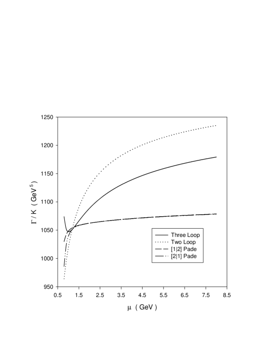
In Figure 5 we have superimposed plots of the reduced rate (10) using

  1. 1.

    Eqs. (4) and (9), the two-loop version of S[x,L]𝑆𝑥𝐿S[x,L] leading to the reduced rate also plotted in Fig. 1,

  2. 2.

    Eq.  (57), the three-loop version of S[x,L]𝑆𝑥𝐿S[x,L] leading to the reduced rate plotted in Fig. 4,

  3. 3.

    S[2|1]superscript𝑆delimited-[]conditional21S^{[2|1]}, as determined via (6265), and

  4. 4.

    S[1|2]superscript𝑆delimited-[]conditional12S^{[1|2]}, as determined via (6669).

The vertical scale of Figure 5 is magnified compared to that of Figs. 1 and 4 in order to accentuate the differences between reduced rates obtained for each of the above scenarios. We observe from Fig.  5 that both Padé-approximant versions of the rate coincide after μ=1.5GeV𝜇1.5GeV\mu=1.5\,{\rm GeV} and are considerably flatter than the rate devolving from the three-loop version of S[x,L]𝑆𝑥𝐿S[x,L]. Indeed, the three-loop reduced rate is itself quite stable, increasing slowly from 1066GeV51066superscriptGeV51066\,{\rm GeV^{5}} to 1180GeV51180superscriptGeV51180\,{\rm GeV^{5}} as μ𝜇\mu increases from 1.5GeV1.5GeV1.5\,{\rm GeV} to 8GeV8GeV8\,{\rm GeV}. Nevertheless, the two Padé approximant versions of S[x,L]𝑆𝑥𝐿S[x,L] vary only minimally over the same range of μ𝜇\mu, increasing from 1058GeV51058superscriptGeV51058\,{\rm GeV^{5}} at μ=1.5GeV𝜇1.5GeV\mu=1.5\,{\rm GeV} to 1079GeV51079superscriptGeV51079\,{\rm GeV^{5}} at μ=8GeV𝜇8GeV\mu=8\,{\rm GeV}. Thus Padé-improvement of the three-loop rate virtually eliminates the residual scale dependence of the naively truncated expression. Such use of Padé approximants to eliminate residual scale dependence is also evident in Fig. 3 of ref. [13] for the buν¯𝑏𝑢superscriptsubscript¯𝜈b\to u\ell^{-}\bar{\nu}_{\ell} rate, and has been previously discussed in the context of the Bjorken sum-rule [21] as well as in more general terms [22]. Of particular interest, however, is the convergence of all four curves in Fig. 5 to virtually the same PMS/FAC point. This convergence lends further support to the PMS/FAC estimates (59), (61) for the reduced rate.

5 Discussion

The entire analysis presented in Section 4 can be repeated using the extreme values b0=8.6subscript𝑏08.6b_{0}=-8.6 and b0=9.2subscript𝑏09.2b_{0}=-9.2, as estimated in [2] (again, see footnote 1), utilising (55) and (56) for the appropriate determinations of three-loop coefficients in conjunction with the known values of a0subscript𝑎0a_{0} and b1subscript𝑏1b_{1} (9). One finds the uncertainty in b0subscript𝑏0b_{0} is reflected in a ±14GeV5plus-or-minus14superscriptGeV5\pm 14\,{\rm GeV^{5}} spread in the PMS/FAC value 1050GeV51050superscriptGeV51050\,{\rm GeV^{5}} for the reduced rate.

Other sources of theoretical uncertainty arise from αs(mτ)=0.33±0.02subscript𝛼𝑠subscript𝑚𝜏plus-or-minus0.330.02\alpha_{s}\left(m_{\tau}\right)=0.33\pm 0.02 [6, 7], mbpole=(4.9±0.1)GeVsuperscriptsubscript𝑚𝑏𝑝𝑜𝑙𝑒plus-or-minus4.90.1GeVm_{b}^{pole}=(4.9\pm 0.1)\,{\rm GeV} [8], and the error that may occur in estimating c0subscript𝑐0c_{0}. We estimate that Padé determinations of c0subscript𝑐0c_{0} are subject to errors comparable to those of Padé determinations of the RG-accessible coefficients c1subscript𝑐1c_{1} and c2subscript𝑐2c_{2}; e.g., |(c1Padec1RG)/c1RG|7%superscriptsubscript𝑐1𝑃𝑎𝑑𝑒superscriptsubscript𝑐1𝑅𝐺superscriptsubscript𝑐1𝑅𝐺percent7\left|\left(c_{1}^{Pade}-c_{1}^{RG}\right)/c_{1}^{RG}\right|\cong 7\%. If we are conservative and estimate the uncertainty of c0subscript𝑐0c_{0} to be double that of c1subscript𝑐1c_{1},

|δc0c0|14%,𝛿subscript𝑐0subscript𝑐0percent14\left|\frac{\delta c_{0}}{c_{0}}\right|\cong 14\%~{}, (70)

the corresponding uncertainty in the reduced rate is ±38GeV5plus-or-minus38superscriptGeV5\pm 38\,{\rm GeV^{5}}. Consequently, our estimate of the purely perturbative three-loop order bcν¯𝑏𝑐superscriptsubscript¯𝜈b\to c\ell^{-}\bar{\nu}_{\ell} rate, as defined by (10), is

ΓpertK=(1050±14±44±115±38)GeV5,superscriptΓ𝑝𝑒𝑟𝑡𝐾plus-or-minus1050144411538superscriptGeV5\frac{\Gamma^{pert}}{K}=\left(1050\pm 14\pm 44\pm 115\pm 38\right)\,{\rm GeV^{5}}~{}, (71)

where the listed theoretical uncertainties respectively devolve from the uncertainty in b0subscript𝑏0b_{0}, αs(mτ)subscript𝛼𝑠subscript𝑚𝜏\alpha_{s}\left(m_{\tau}\right), mbpolesuperscriptsubscript𝑚𝑏𝑝𝑜𝑙𝑒m_{b}^{pole}, and c0subscript𝑐0c_{0}.

Nonperturbative (NP) contributions to the rate may be extracted from Eq. (5.8) of [23], and correspond to the following additional contributions to the series S[x,L]𝑆𝑥𝐿S[x,L]:

ΔSNP=λ1+3λ22mb26(1mc2mb2)4λ2mb2F(mc2mb2),Δsuperscript𝑆𝑁𝑃subscript𝜆13subscript𝜆22superscriptsubscript𝑚𝑏26superscript1superscriptsubscript𝑚𝑐2superscriptsubscript𝑚𝑏24subscript𝜆2superscriptsubscript𝑚𝑏2𝐹superscriptsubscript𝑚𝑐2superscriptsubscript𝑚𝑏2\Delta S^{NP}=\frac{\lambda_{1}+3\lambda_{2}}{2m_{b}^{2}}-\frac{6\left(1-\frac{m_{c}^{2}}{m_{b}^{2}}\right)^{4}\lambda_{2}}{m_{b}^{2}\,F\left(\frac{m_{c}^{2}}{m_{b}^{2}}\right)}~{}, (72)

where the form factor F𝐹F is given by (2) and where

0.5GeV2λ10,λ2=0.12GeV2.formulae-sequence0.5superscriptGeV2subscript𝜆10subscript𝜆20.12superscriptGeV2-0.5\,{\rm GeV^{2}}\leq\lambda_{1}\leq 0~{},~{}\lambda_{2}=0.12\,{\rm GeV^{2}}~{}. (73)

This additional NP contribution entails a 6%similar-toabsentpercent6\sim 6\% reduction in the reduced rate (71):

ΓK=ΓpertK(58.5±5.5)GeV5=(992±217)GeV5,Γ𝐾superscriptΓ𝑝𝑒𝑟𝑡𝐾plus-or-minus58.55.5superscriptGeV5plus-or-minus992217superscriptGeV5\frac{\Gamma}{K}=\frac{\Gamma^{pert}}{K}-\left(58.5\pm 5.5\right)\,{\rm GeV^{5}}=\left(992\pm 217\right)\,{\rm GeV^{5}}~{}, (74)

where the independent sources of uncertainty in (71) and in the intermediate step of (74) have been combined additively.

If we identify the predicted bcν¯𝑏𝑐superscriptsubscript¯𝜈b\to c\ell^{-}\bar{\nu}_{\ell} decay rate with the inclusive semileptonic process BXcν¯𝐵subscript𝑋𝑐superscriptsubscript¯𝜈B\to X_{c}\ell^{-}\bar{\nu}_{\ell} [=e𝑒\ell=e or μ𝜇\mu, but not their sum], we can then relate the aggregate theoretical uncertainty in (74) to the concomitant theoretical uncertainty in the determination of |Vcb|subscript𝑉𝑐𝑏\left|V_{cb}\right|:

|Vcb|=[192π3BR(BXcν¯)GF2τB[(992±217)GeV5]]1/2subscript𝑉𝑐𝑏superscriptdelimited-[]192superscript𝜋3Planck-constant-over-2-piBR𝐵subscript𝑋𝑐superscriptsubscript¯𝜈superscriptsubscript𝐺𝐹2subscript𝜏𝐵delimited-[]plus-or-minus992217superscriptGeV512\left|V_{cb}\right|=\left[\frac{192\pi^{3}\hbar\,{\rm BR}\left(B\to X_{c}\ell^{-}\bar{\nu}_{\ell}\right)}{G_{F}^{2}\tau_{{}_{B}}\left[\left(992\pm 217\right)\,{\rm GeV^{5}}\right]}\right]^{1/2} (75)

To factorize experimental and theoretical uncertainties, we employ recent central values for the average B𝐵B lifetime τBsubscript𝜏𝐵\tau_{{}_{B}} [25] and the BXceν¯e𝐵subscript𝑋𝑐superscript𝑒subscript¯𝜈𝑒B\to X_{c}e^{-}\bar{\nu}_{e} branching ratio [26] to rewrite (75) in the following form:

|Vcb|=(0.04530.0043+0.0060)(1.564×10¹²sτB)1/2(BR(BXcν¯)0.1105)1/2subscript𝑉𝑐𝑏subscriptsuperscript0.04530.00600.0043superscript1.564superscript1012ssubscript𝜏𝐵12superscriptBR𝐵subscript𝑋𝑐superscriptsubscript¯𝜈0.110512\left|V_{cb}\right|=\left(0.0453^{+0.0060}_{-0.0043}\right)\,\left(\frac{1.564\times 10^{-12}\,{\rm s}}{\tau_{{}_{B}}}\right)^{1/2}\,\left(\frac{{\rm BR}\left(B\to X_{c}\ell^{-}\bar{\nu}_{\ell}\right)}{0.1105}\right)^{1/2} (76)

The first factor in (76) reflects the summed theoretical uncertainties in (74), which are separately broken down in (71). We have been conservative in identifying and assessing the magnitude of each such independent source of error— the theoretical uncertainty estimated from a (truncated) two-loop calculation of the bcν¯𝑏𝑐superscriptsubscript¯𝜈b\to c\ell^{-}\bar{\nu}_{\ell} rate should be larger than that obtained by us in (76).

Note also that we can compare our Γpert/K=1050GeV5superscriptΓ𝑝𝑒𝑟𝑡𝐾1050superscriptGeV5\Gamma^{pert}/K=1050\,{\rm GeV^{5}} central value estimate (71) for the reduced rate (exclusive of NP effects) with the corresponding estimate one would obtain using low-scale masses [2]:333The 𝒪(αs2)𝒪superscriptsubscript𝛼𝑠2{\cal O}\left(\alpha_{s}^{2}\right) coefficient in (77) [A. Czarnecki, personal communication] differs slightly from the value 2.65±0.4plus-or-minus2.650.4-2.65\pm 0.4 appearing in ref. [2].

ΓpertK=m~b5F(m~c2m~b2)[11.14αs(m~bm~c)π(3.5±0.3)(αs(m~bm~c)π)2].superscriptΓ𝑝𝑒𝑟𝑡𝐾superscriptsubscript~𝑚𝑏5𝐹superscriptsubscript~𝑚𝑐2superscriptsubscript~𝑚𝑏2delimited-[]11.14subscript𝛼𝑠subscript~𝑚𝑏subscript~𝑚𝑐𝜋plus-or-minus3.50.3superscriptsubscript𝛼𝑠subscript~𝑚𝑏subscript~𝑚𝑐𝜋2\frac{\Gamma^{pert}}{K}=\tilde{m}_{b}^{5}\,F\left(\frac{\tilde{m}_{c}^{2}}{\tilde{m}_{b}^{2}}\right)\left[1-1.14\frac{\alpha_{s}\left(\sqrt{\tilde{m}_{b}\tilde{m}_{c}}\right)}{\pi}-\left(3.5\pm 0.3\right)\left(\frac{\alpha_{s}\left(\sqrt{\tilde{m}_{b}\tilde{m}_{c}}\right)}{\pi}\right)^{2}\right]~{}. (77)

If we utilise the low-scale mass values m~b=4.64GeVsubscript~𝑚𝑏4.64GeV\tilde{m}_{b}=4.64\,{\rm GeV}, m~c=1.25GeVsubscript~𝑚𝑐1.25GeV\tilde{m}_{c}=1.25\,{\rm GeV}, as quoted in [2] from ref. [24] and find via devolution from αs(mτ)=0.33subscript𝛼𝑠subscript𝑚𝜏0.33\alpha_{s}\left(m_{\tau}\right)=0.33 that αs(m~bm~c)/π=0.091subscript𝛼𝑠subscript~𝑚𝑏subscript~𝑚𝑐𝜋0.091\alpha_{s}\left(\sqrt{\tilde{m}_{b}\tilde{m}_{c}}\right)/\pi=0.091, we observe that the rate predicted via (77) is 1097GeV51097superscriptGeV51097\,{\rm GeV^{5}}, an answer in surprisingly good agreement with our 1050GeV51050superscriptGeV51050\,{\rm GeV^{5}} three-loop estimate in the pole-mass renormalization scheme.

We conclude by noting that the RG equation (6, 7) may be used to determine additional higher-order corrections to the decay rate (1). The leading-log corrections to all orders in x𝑥x are determined by the one-loop β𝛽\beta-function; next-to-leading-log corrections to all orders in x𝑥x are determined by the two-loop β𝛽\beta-function etc. Although we have made use of RG-invariance to 𝒪(x3)𝒪superscript𝑥3{\cal O}\left(x^{3}\right) in present work, it is in fact possible to incorporate these logarithmic corrections to all subsequent orders. The full exploitation of RG-invariance within perturbative-QCD expressions for physical processes is presently under study.

Acknowledgments: We are grateful for the hospitality of the KEK Theory Group, where this research was conducted with financial support from the International Opportunity Fund of the Natural Sciences and Engineering Research Council of Canada (NSERC) and the International Collaboration Programme 2001 of Enterprise Ireland.

References

  • [1] A. Czarnecki, Phys. Rev. Lett. 76 (1996) 4124;
    A. Czarnecki and K. Melnikov, Phys. Rev. Lett. 78 (1997) 3630;
    A. Czarnecki, K.  Melnikov, and N. Uraltsev, Phys. Rev. D 57 (1998) 1769.
  • [2] A. Czarnecki and K. Melnikov Phys. Rev. D 59 (1999) 014036.
  • [3] T. van Ritbergen, Phys. Lett. B 454 (1999) 353.
  • [4] P.M. Stevenson, Phys. Rev. D 23 (1981) 2916.
  • [5] G. Grunberg, Phys. Lett. B 95 (1980) 70 and Phys. Rev. D 29 (1984) 2315.
  • [6] ALEPH Collaboration (R. Barate et al.), Eur. Phys. J. C 4 (1998) 409;
    G. Cvetic and T. Lee, hep-ph/0101297;
    C.J. Maxwell and A. Mirjalili, hep-ph/0103164.
  • [7] T.G. Steele and V. Elias, Mod. Phys. Lett. A 13 (1998) 3151.
  • [8] A.H. Hoang, Phys. Rev. D 61 (2000) 034005 and D 59 (1999) 014039.
  • [9] T. van Ritbergen, J.A.M. Vermaseren, and S.A. Larin, Phys. Lett. B 400 (1997) 379.
  • [10] N. Gray, D.J. Broadhurst, W. Grafe, and K. Schilcher, Z. Phys. C 48 (1990) 673;
    D.J. Broadhurst, N. Gray, and K. Schilcher, Z. Phys. C 52 (1991) 111;
    J. Fleischer, F. Jegerlehner, O.V. Tarosov, and O.L. Veretin, Nucl. Phys. B 539 (1999) 671;
    K.G. Chetyrkin and M. Steinhauser, Nucl. Phys. B 573 (2000) 617 and Phys. Rev.  Lett. 83 (1999) 4001.
  • [11] A. Hoang, Z. Ligeti, and A.V. Manohar, Phys. Rev. D 59 (1999) 074017.
  • [12] K.G. Chetyrkin, Phys. Lett. B 404 (1997) 161.
  • [13] M.R. Ahmady, F.A. Chishtie, V. Elias, and T.G. Steele, Phys. Lett. B 479 (2000) 201.
  • [14] J. Ellis, M. Karliner, and M.A. Samuel, Phys. Lett. B 400 (1997) 176.
  • [15] I. Jack, D.R.T. Jones, and M.A. Samuel, Phys. Lett. B 407 (1997) 143;
    I. Jack, D.R.T. Jones, and A. Pickering, Phys. Lett. B 435 (1998) 61.
  • [16] F.A. Chishtie and V. Elias, Phys. Lett. B 499 (2001) 270.
  • [17] V. Elias, T.G. Steele, F. Chishtie, R. Migneron, and K. Sprague, Phys. Rev. D 58 (1998) 116007;
    V. Elias, F.A. Chishtie, and T.G. Steele, J. Phys. G 26 (2000) 1239.
  • [18] F.A. Chishtie, V. Elias, and T.G. Steele, J. Phys. G 26 (2000) 93.
  • [19] F.A. Chishtie and V. Elias, hep-ph/0107052.
  • [20] F. Chishtie, V. Elias, and T.G. Steele, Phys. Rev. D 59 (1999) 105013.
  • [21] J. Ellis, E. Gardi, M. Karliner, and M.A. Samuel, Phys. Lett. B 366 (1996) 4380 and Phys. Rev. D 54 (1996) 6986.
  • [22] E. Gardi, Phys. Rev. D 56 (1997) 68.
  • [23] E. Bagan, P. Ball, V.M. Braun, and P. Godzinsky, Nucl. Phys. B 432 (1994) 3.
  • [24] I.I.Y. Bigi, M.A. Shifman, and N. Uraltsev, Ann. Rev. Nucl. Part. Sci. 47 (1997) 591.
  • [25] M. Battaglia, Nucl. Phys. Proc. Suppl. 96 (2001) 443.
  • [26] BELLE double-lepton tag data reported by H. Ishino at YITP (Kyoto) Conference, July 10, 2001.
Refer to caption
Figure 1: Renormalization scale (μ𝜇\mu) dependence of the two-loop reduced rate Γ/KΓ𝐾\Gamma/K in the pole mass scheme.
Refer to caption
Figure 2: Renormalization scale (μ𝜇\mu) dependence of the two-loop reduced rate Γ/KΓ𝐾\Gamma/K in the MS¯¯MS\overline{\rm MS} scheme. In the MS¯¯MS\overline{\rm MS} scheme, mb(μ)subscript𝑚𝑏𝜇m_{b}(\mu) is obtained from the four-loop nf=4subscript𝑛𝑓4n_{f}=4 anomalous mass dimension [12] using mb(mb)=4.2GeVsubscript𝑚𝑏subscript𝑚𝑏4.2GeVm_{b}\left(m_{b}\right)=4.2\,{\rm GeV} [8] as a reference value.
Refer to caption
Figure 3: The quantity ΔΔ\Delta measuring the sum of the relative errors in the Padé estimate (43,44) of the RG-accessible three-loop coefficients {c1,c2}subscript𝑐1subscript𝑐2\{c_{1},c_{2}\} plotted as a function of the error-formula parameter k𝑘k (27). The location of the curve’s minimum represents the value of k𝑘k leading to an optimized Padé estimate.
Refer to caption
Figure 4: Renormalization scale (μ𝜇\mu) dependence of the three-loop reduced rate Γ/KΓ𝐾\Gamma/K in the pole mass scheme. The PMS point is represented by the local minimum of the curve.
Refer to caption
Figure 5: Scale dependence of different estimates of the reduced rate in the pole scheme. The solid curve represents the three-loop estimate presented in Fig. 4, and the dotted curve represents the two-loop estimate also presented in Fig. 1. The [1|2]delimited-[]conditional12[1|2] and [2|1]delimited-[]conditional21[2|1] Padé approximants obtained from the three-loop estimated rate are represented by the dashed curves which overlap almost completely above μ=1.5GeV𝜇1.5GeV\mu=1.5\,{\rm GeV}. The PMS point is represented by the local minimum of the three-loop curve, and the FAC point occurs at the intersection of the two- and three-loop curves. Note the convergence of all the estimates near the FAC/PMS points.