PACS numbers: 11.55.Bq, 14.40.Cs, 12.39.Fe
Key words: $\pi\pi$ scattering; Padé approximation; Chiral perturbation theory

The chiral perturbation theory [1] is a powerful tool in studying strong interaction physics at low energies. The principle of chiral perturbation theory is that it incorporates the global symmetry of the QCD Lagrangian – the spontaneously broken chiral symmetry – into the effective Lagrangian, and directly deals with the physical states – the pseudo-Goldstone bosons – as the physical degrees of freedom in the effective Lagrangian. The physical amplitude is calculated by a perturbative expansion in powers of the light quark masses and the external momentum, and unitarity is respected perturbatively. As the external momentum increases, however, the chiral expansion diverges rapidly and the unitarity condition is badly violated. To remedy such a situation, the Padé approximation has been used to improve the behavior of chiral amplitudes at higher energies, which has stimulated revived interests in the recent literature (see for example [2] –[6]). One of the cost in using Padé approximation is the violation of crossing symmetry which has also been discussed in the recent literature (see for example Refs. [7, 8] and [3]).

For the $\pi\pi\rightarrow\pi\pi$ scattering process, the isospin amplitudes in the s channel can be decomposed as [10],

$$T^{I=0}(s,t,u) = 3A(s,t,u)+A(t,u,s)+A(u,s,t)\ ,$$

$$T^{I=1}(s,t,u) = A(t,u,s)-A(u,s,t)\ ,$$ (1)

$$T^{I=2}(s,t,u) = A(t,u,s)+A(u,s,t)\ ,$$

as a result of the generalized Bose statistics and crossing symmetry. In $SU(2)\times SU(2)$ chiral perturbation theory (ChPT) to one loop [9] we have,

$$A(s,t,u) = {s-m_{\pi}^{2}\over F_{\pi}^{2}}+A_{1}(s,t,u)+A_{2}(s,t,u)+O(E^{6}),$$

$$A_{1}(s,t,u) = {1\over 6F_{\pi}^{4}}\{3(s^{2}-m_{\pi}^{4}){\bar{J}}(s)+\left[t(t-u)-2m_{\pi}^{2}t+4m_{\pi}^{2}u-2m_{\pi}^{4}\right]{\bar{J}}(t)$$

$$+\left[u(u-t)-2m_{\pi}^{2}u+4m_{\pi}^{2}t-2m_{\pi}^{4}\right]{\bar{J}}(u)\},$$

$$A_{2}(s,t,u) = {1\over 96\pi^{2}F_{\pi}^{4}}\{2(\bar{l}_{1}-{4\over 3})(s-2m_{\pi}^{2})^{2}+(\bar{l}_{2}-{5\over 6})\left[s^{2}+(t-u)^{2}\right]-12m_{\pi}^{2}s$$ (2)

$$+15m_{\pi}^{4}+12m_{\pi}^{2}(s-m_{\pi}^{2})\bar{l}_{4}-3m_{\pi}^{4}\bar{l}_{3}\}$$

where $F_{\pi}=93.3$MeV is the pion decay constant and the function ${\bar{J}}(s)$ is defined as

$${\bar{J}}(s) = {1\over 16\pi^{2}}\left[\rho{\rm ln}\left({\rho-1\over\rho+1}\right)+2\right],$$

$$\rho(s) = \sqrt{1-{4m_{\pi}^{2}\over s}}\ .$$ (3)

In Ref. [9] the $\bar{l}_{i}$ parameters are taken to be

$$\bar{l}_{1}=-0.62\pm 0.94\ ,\,\,\,\bar{l}_{2}=6.28\pm 0.48\ ,\,\,\,\bar{l}_{3}=2.9\pm 2.4\ ,\,\,\,\bar{l}_{4}=4.3\pm 0.9$$ (4)

determined from low energy experiments.

The partial wave expansion of the isospin amplitudes is written as

$$T^{I}(s,t,u) = 32\pi\sum_{J}(2J+1)P_{J}(\cos\theta){T^{I}_{J}}(s)\ ,$$ (5)

where, for $\pi\pi$ scatterings, the sum is over even(odd) values of $J$ for even(odd) values of $I$ because of the restriction of Bose statistics. The inverse expression is

$$T_{J}^{I}(s) = {1\over 64\pi}\int^{1}_{-1}d{\cos\theta}\,P_{J}(cos\theta)T^{I}(s,t,u)\ ,$$

$$\cos\theta = 1+{{2t}\over{s-4m_{\pi}^{2}}}\ ,$$ (6)

$$u = 4m_{\pi}^{2}-s-t\ .$$

The partial wave amplitudes in ChPT expanded to $O(p^{4})$ are,

$$T^{I}_{J}(s)=T^{I}_{J,2}(s)+T^{I}_{J,4}(s)\ ,$$ (7)

where $T^{I}_{J,2}(s)$ and $T^{I}_{J,4}(s)$ represent terms of order $O(p^{2})$ and $O(p^{4})$, respectively. The $T^{I}_{J,2}(s)$ amplitudes can be rigorously derived from current algebra and are model independent. The [1,1] Padé approximation to the partial wave amplitudes is,

$$T^{I[1,1]}_{J}(s)={{T^{I}_{J,2}(s)}\over{1-{T^{I}_{J,4}(s)/T^{I}_{J,2}(s)}}}\quad.$$ (8)

From perturbative unitarity in ChPT we have

$${\rm Im}T^{I}_{J,4}(s) = \rho|T^{I}_{J,2}(s)|^{2}\ ,\,\,(4m_{\pi}^{2}<s<16m_{\pi}^{2})\ .$$ (9)

With this relation, it is easy to prove that the [1,1] Padé approximants given in Eq. (8) satisfy elastic unitarity:

$${\rm Im}T^{I[1,1]}_{J}(s)=\rho|T^{I[1,1]}_{J}(s)|^{2}\quad,$$ (10)

and it is well known that the phase shifts they predict are considerably improved comparing with the perturbation results. However, the total amplitude

$$T(s,t,u)=32\pi\sum_{J}(2J+1)P_{J}(cos\theta){T_{J}}(s)\ ,$$ (11)

has certain crossing properties which are lost in the amplitude defined by

$$T^{P}(s,t,u)\equiv 32\pi\sum_{J}(2J+1)P_{J}(cos\theta){T^{[1,1]}_{J}}(s)\ ,$$ (12)

by violating the so called Balachandran-Nuyts-Roskies relations, as discussed recently in Refs. [7, 8].

The Padé approximation not only gives an improved prediction to the $\pi\pi$ scattering phases comparing to the perturbative results, but also it predicts the correct physical resonances on a qualitative level. For example in the amplitude $T^{0[1,1]}_{0}(s)$, on the second sheet of the complex $s$ plane one finds the $\sigma$ resonance with $M_{\sigma}=430$MeV and $\Gamma_{\sigma}=456$MeV,  and the $\rho$ resonance in the IJ=11 channel: $M_{\rho}=708$MeV and $\Gamma_{\rho}=119$MeV which should be compared with the experimental value $M_{\rho}=769$MeV and $\Gamma_{\rho}=150$MeV. Actually, the quality of the Padé approximants can be much improved by tuning the $\bar{l}_{i}$ parameters within reasonable ranges, that is to fit the global phase shifts while the $\bar{l}_{i}$ parameters are still consistent with the parameters constrained by low energy experiments. This remarkable improvement is possible, as pointed out in Refs. [5, 6]. Inspired by this approach (often called unitarized chiral approach in the literature), we also made a global fit to the experimental phase shifts using the [1,1] Padé amplitudes in Eq. (8). In our fit the experimental data are taken from Refs. [12] – [15], especially we also include the newest E865 Collaboration data from $K_{e4}$ decays [16]. We fit the IJ=11 and 20 data up to $\sqrt{s}=1GeV$ and the IJ=00 data up to $\sqrt{s}=700$MeV.  The fit quality is impressive, as can be seen in Fig 1.

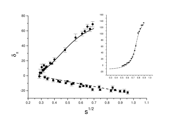
Figure 1: The global fit in IJ=00, 11 and 20 channels, using the [1,1] Padé approximants and the procedure described in the text.

The resulting values of the $\bar{l}_{i}$ parameters corresponding to the minimized $\chi^{2}$ are as follows,

$$\bar{l}_{1}=-0.485\ ,\,\,\,\bar{l}_{2}=5.696\ ,\,\,\,\bar{l}_{3}=16.136\ ,\,\,\,\bar{l}_{4}=3.650\ .$$ (13)

Notice that in the above fit the $\bar{l}_{3}$ parameter is much larger than that in Eq. (4) and the value in Ref. [5]. This is not a serious problem as we found in the fit that though the minimization of the $\chi^{2}$ prefers a large value of $\bar{l}_{3}$ but it is not sensitive to $\bar{l}_{3}$. Another fact which is worth pointing out is that the chiral estimate on $\bar{l}_{3}$ is crude and is subject to large uncertainties [17]. The physical resonances obtained from our global fit are, $M_{\rho}=751$MeV, $\Gamma_{\rho}=144$MeV and $M_{\sigma}=449$MeV, $\Gamma_{\sigma}=482$MeV. The scattering length parameters in the IJ=00 and 20 channels are found to be $a_{0}^{0}=0.194$ and $a^{2}_{0}=-0.044$ which are reasonable as comparing with the experimental results.

Though successfully predicting the existence of the $\sigma$ and the $\rho$ resonances qualitatively or even quantitatively for the latter, it is well known that the Padé approximation encounters severe problems in theory aspects. One of which is the generation of dubious poles on the complex $s$ plane, as listed in tables 1 and 2,  except for those physically accepted.

	Pole status	Re[$s_{pole}$] (MeV)	Im[$s_{pole}$] (MeV)	residue ($GeV^{2}$)
IJ=11	$\rho$	708 (M)	119 ($\Gamma$)	-0.07+0.15i
	$\sigma$	430 (M)	456 ($\Gamma$)	-0.19-0.23i
IJ=00	BS1	$0.618m_{\pi}^{2}$		$-5\times 10^{-5}$
	VS1	$0.621m_{\pi}^{2}$		$6.2\times 10^{-5}$
	PSR	$-81.1m_{\pi}^{2}$	$60.6m_{\pi}^{2}$	-4.76-4.50i
	BS1	$1.97528m_{\pi}^{2}$		$6\times 10^{-7}$
IJ=20	VS1	$1.97525m_{\pi}^{2}$		$-6\times 10^{-7}$
	VS2	$0.0495m_{\pi}^{2}$		$1.8\times 10^{-3}$
	PSR	$133.8m_{\pi}^{2}$	$483.4m_{\pi}^{2}$	-26.27+4.09i

Table 1: Resonances, physical sheet resonances (PSR), bound states (BS) and virtual states (VS) as predicted by Padé approximation on the complex $s$ plane using the $\bar{l}_{i}$ parameters from Ref. [9]. The pole position $s_{pole}=(M+i\Gamma/2)^{2}$. Here the residue of a second sheet pole means the residue of the corresponding pole in $1/S$.

	Pole status	Re[$s_{pole}$] (MeV)	Im[$s_{pole}$] (MeV)	residue ($GeV^{2}$)
IJ=11	$\rho$	751 ($M$)	144 ($\Gamma$)	-0.10+0.19i
	$\sigma$	449 ($M$)	482 ($\Gamma$)	-0.16-0.27i
IJ=00	BS1	$0.372m_{\pi}^{2}$		$-7\times 10^{-5}$
	VS1	$0.376m_{\pi}^{2}$		$8\times 10^{-5}$
	PSR	$-68.5m_{\pi}^{2}$	$47.1m_{\pi}^{2}$	-3.56-3.55i
	BS1	$2.17832m_{\pi}^{2}$		$3\times 10^{-5}$
IJ=20	VS1	$2.17701m_{\pi}^{2}$		$-3\times 10^{-5}$
	VS2	$0.0372m_{\pi}^{2}$		$1.4\times 10^{-3}$
	PSR	$106.0m_{\pi}^{2}$	$306.8m_{\pi}^{2}$	-16.45+2.62i

Table 2: Resonances, physical sheet resonances (PSR), bound states (BS) and virtual states (VS) as predicted by Padé approximation on the complex $s$ plane, using the $\bar{l}_{i}$ parameters obtained from the global fit to the phases in the IJ=00,20,11 channels as described in the text. The pole position $s_{pole}=(M+i\Gamma/2)^{2}$. Here the residue of a second sheet pole means the residue of the corresponding pole in $1/S$.

We categorize these dubious poles into 3 classes: the first contains the bound state pole and the accompanying virtual state pole denoted as BS₁ and VS₁ respectively (the latter corresponds to the zero in the physical sheet below threshold) in the IJ=00,20 channels. The positions of the pole and the accompanying zero are very close to each other. The second includes the resonance poles found in the physical sheet (denoted as PSR), and the third class is for the virtual state (denoted as VS₂) near $s=0$ found in the IJ=20 channel.

There are two reasons to ignore the first class poles. The first reason is that they have very tiny residues and can be safely ignored numerically. The second reason is that they can be tuned to disappear totally by varying the $\bar{l}_{i}$ parameters in the reasonable range. To see this more clearly we recall that the $S$ matrix of the [1,1] Padé approximant takes the following form,

$$S^{[1,1]}=\frac{T_{2}-T_{4}^{*}}{T_{2}-T_{4}}=\frac{T_{2}-{\rm Re}T_{4}+i\rho(T_{2})^{2}}{T_{2}-{\rm Re}T_{4}-i\rho(T_{2})^{2}}\ ,$$ (14)

where the spin and isospin indices are dropped for simplicity. A virtual state is an $S$ matrix zero located on the real axis below the threshold which requires $T_{2}=T_{4}^{*}$ whereas the bound state pole requires $T_{2}=T_{4}$. Therefore the bound state pole and the virtual state disappear simultaneously if the following requirements are met,

$${\rm Im}T_{4}=0\ ,\,\,\,\,{\rm Re}T_{4}=T_{2}\ .$$ (15)

Since ${\rm Im}T_{4}=\rho(T_{2})^{2}$ from perturbative unitarity the first condition in Eq. (15) implies that the bound state pole and the virtual state pole cancel each other when they move towards the Adler zero position for the lowest order partial wave amplitude. As a consequence, the Adler zero of the Padé approximant is still there which coincides with the one of the lowest order partial wave amplitude, but the order of the zero decreases from two to one (the second order Adler zero is unnecessary from theoretical point of view). The second condition of Eq. (15), which now reads ${\rm Re}T_{4}=0$, affords a constraint that those $\bar{l}_{i}$ parameters have to obey.  To cancel the bound state in the IJ=20 channel, we can for example choose the following set of $\bar{l}_{i}$: $\bar{l}_{1}=-0.5,\bar{l}_{2}=5.3,\bar{l}_{3}=3.7,\bar{l}_{4}=4.0$, satisfying Eq. (16) numerically which fit the experimental values of $m_{\rho}$ and $\Gamma_{\rho}$ well. For these $\bar{l}_{i}$ parameters the experimental phase shifts of three channels IJ=00,20 and 11 are also fitted well. Similar situation happens in the IJ=00 channel. But when we try to cancel the bound states both in IJ=00 and IJ=20 channels simultaneously, it is difficult to find a set of $\bar{l}_{i}$ parameters within reasonable ranges to agree well with the experimental phase shifts simultaneously in three channels. We ascribe this difficulty to the non-perfectness of the Padé approximation itself.

The existence of the physical sheet resonances violate causality and must be a false prediction of Padé approximation. One may argue that such kind of false poles locate very far from the physical region and the region where ChPT is valid (inside the circle $|s|<<1$GeV²), and therefore the Padé approximation is still acceptable numerically in phenomenology. However a careful analysis just reveals the opposite. As can be seen from tables 1 and 2 the residues of the PSRs are usually very large that in some cases it strongly plagues the prediction of the Padé approximation. To see this more clearly, taking the IJ=20 channel for example, we recall the following dispersion relations [11, 18]:

$$\cos(2\delta_{\pi 0}^{2}) = 1+{(s-4m_{\pi}^{2})\over 2\pi}\int_{-\infty}^{0}{{\rm Im}(S(s^{\prime})+{1\over S(s^{\prime})})\over(s^{\prime}-s)(s^{\prime}-4m_{\pi}^{2})}ds^{\prime},$$ (18)

$$\sin(2\delta_{\pi 0}^{2}) = \rho(s)\left[2a^{2}_{0}+{(s-4m_{\pi}^{2})\over 2\pi}\int_{-\infty}^{0}{{\rm Im}({1\over i\rho}(S(s^{\prime})-{1\over S(s^{\prime})}))\over(s^{\prime}-s)(s^{\prime}-4m^{2}_{\pi})}ds^{\prime}\right].$$ (19)

These two equations are obtained by assuming no pole exists on both sheets. But pole contributions from different sheets can be added to the above equations easily. The left hand integrals can be evaluated by using the expressions obtained from the Padé approximant $T^{2}_{0}$. The left hand side of Eqs. (18) and (19) can be directly evaluated from the Padé amplitudes in the physical region. The right hand side of Eqs. (18) and (19) separate different type of contributions, i.e., from cuts, resonances, bound states, virtual states or physical sheet resonances. It is clearly seen in Fig. 2, that the contribution from the left hand integral in Eq. (18) deviates far from the experimental value. Only after adding the physical sheet resonance in Eq. (18) may we reproduce the phase in the physical region. Though in Eq. (19) the left hand integral works rather well numerically, the predictions of Padé approximants on poles and cuts become no longer trustworthy quantitatively, in the situation when there exist physical sheet resonances with large residues.

         

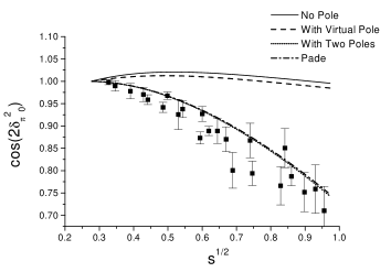
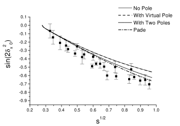
Figure 2: Various contributions to $\cos(2\delta^{2}_{\pi 0})$ and $\sin(2\delta^{2}_{\pi 0})$ in the IJ=20 channel. Solid lines represent only the left hand integral contributions in Eq. (18) and Eq. (19). In the dashed line the virtual state (VS₂) contribution is added; in the dotted line the contributions from both the virtual state and the physical sheet resonance are added. The dotted line numerically coincides with the dot-dashed line as it should be, the latter is obtained by evaluating the Padé amplitude in the physical region, using the $\bar{l}_{i}$ parameters from Ref. [9].

From the above discussions we realize that the existence of the physical sheet resonance plagues the predictive power of the Padé approximant $T^{2}_{0}$, at quantitative level. Similar things happen also in the IJ=00 channel.  Fortunately Padé approximants still work qualitatively in the sense that it correctly predicts the existence of the physical resonances, like $\sigma$ and $\rho$. In here it is worth emphasizing that the virtual state VS₂ in the IJ=20 channel may be physical. The residue of such pole, though very small, is much larger than the residues of BS₁ and VS₁, and it improves the $r.h.s.$ of Eq. (18). There is a simple reason for the existence of such a pole which does not rely on the detailed form of the Padé approximant $T^{2}_{0}$. To understand this, we recall that around the bound state pole at $s=s_{B}$ the $S$ matrix can be expanded as $r/(s-s_{B})+C+O((s-s_{B}))$ where $C$ is a constant. The accompanying zero will occur at $s_{0}\simeq s_{B}-r/C$ for any non zero value of $C$. This simple mechanism explains the pair production of BS₁ and VS₁. The reason for the generation of VS₂ is similar. Remember that $S=1+2i\rho T$ and $i\rho$ is purely real and negative when $0<s<4m_{\pi}^{2}$. When $s\rightarrow 0$ from positive side $i\rho\rightarrow-\infty$ therefore if $T(0_{+})$ is positive then $S(0_{+})\rightarrow-\infty$. But since $S(4m_{\pi}^{2})=1$ therefore the $S$ matrix must go through a zero (at least once) located somewhere between $s=0+$ and $s=4m_{\pi}^{2}$. It happens that the [1,1] Padé approximation gives a negative value to $T_{0}^{0[1,1]}(0_{+})$ and $T_{1}^{1[1,1]}(0_{+})$, but a positive value to $T_{0}^{2[1,1]}(0_{+})$. From this analysis we realize that the existence of the virtual state VS₂ is a consequence of more general situation ($T(0_{+})>0$) than that of the concrete form of the Padé approximant $T^{2[1,1]}_{0}$. In here the signs of the Padé amplitudes $T^{0[1,1]}_{0}(0_{+})$, $T^{1[1,1]}_{1}(0_{+})$ and $T^{2[1,1]}_{0}(0_{+})$ coincide with the signs of the lowest order amplitudes $T^{0}_{0,2}(0_{+})$, $T^{1}_{1,2}(0_{+})$ and $T^{2}_{0,2}(0_{+})$, respectively, and the lowest order amplitudes are unambiguous predictions from current algebra. The coincidence of the sign simply reflects the fact that the lowest order amplitudes dominate at $s\sim 0$, as can be clearly seen in Fig. 3. Though the virtual state may really exist, its effect may be very small due to its small coupling, as indicated by tables 1 and 2.

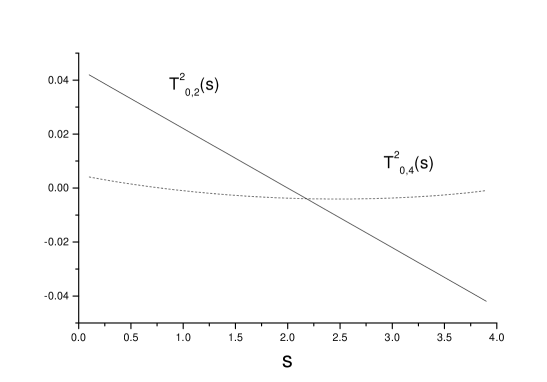
Figure 3: $T^{2}_{0,2}$ and $T^{2}_{0,4}$ amplitudes using $l_{i}$ parameters obtained from our global fit to the Padé amplitudes in IJ=00, 20 and 11 channels. The bound state pole locates at the point where the two amplitudes meet.

To conclude, the dispersion relations set up in Refs. [11] and [18] enable us to examine explicitly contributions from different types of dynamical singularities – the resonances, the left–hand cuts, and the bound states or virtual states – to the phase shifts. Hence a critical examination on the Padé approximation becomes possible. We find that even though the Padé approximation can give a reasonable global fit to the $\pi\pi$ scattering phase shifts, the contribution to the phase shifts can be largely from disastrous physical sheet resonances in some situations. In such cases the other predictions of the Padé amplitudes become unreliable either, at least at quantitative level. However we argue that in the IJ=20 channel the virtual state close to $s=0$ as predicted by the Padé approximation is a consequence of more general conditions and seems to exist physically.

References

- [1] J. Gasser and H. Leutwyler, Ann. of Phys. 158 (1984)142 and referrences therein;
- [2] T. N. Truong, Phys. Rev. Lett. 61 (1988)2526.
- [3] A. Dobado and J. R. Pelaez, Phys. Rev. D56 (1997) 3057.
- [4] T. Hannah, Phys. Rev. D60 017502 (1999).
- [5] F. Guerrero and J. A. Oller, Nucl. Phys. B537 (1999) 459.
- [6] J. A. Oller, E. Oset and A. Ramos, Prog. Part. Nucl. Phys. 45 (2000) 157.
- [7] M. Boglione and M. R. Pennington. Z. Phys. C75 (1997) 113.
- [8] I. P. Cavalcante and J. Sá Borges, hep-ph/0101037.
- [9] J. Gasser and U. Meissner, Nucl. Phys. B357 (1991) 90.
- [10] B. R. Martin, D. Morgan and G. Shaw, – , Academic press, 1976, London.
- [11] Zhiguang Xiao and H. Q. Zheng, hep-ph/0011260, to appear in Nucl. Phys. A; hep-ph/0103042; hep-ph/0107188.
- [12] S. D. Protopopescu et al., Phys. Rev. D7 (1973) 1279.
- [13] G. Grayer et al., Nucl. Phys. B75 (1974) 189; W. Ochs, Ph.D. thesis, Munich Univ., 1974.
- [14] W. Maenner, in – 1974 (Boston), Proceedings of the fourth International Conference on Meson Spectroscopy, edited by D. A. Garelick, AIP Conf. Proc. No. 21 (AIP, New York, 1974).
- [15] L. Rosselet et al., Phys. Rev. D15 (1977) 574.
- [16] P. Truoel (E865 Collaboration), hep-ex/0012012.
- [17] G. Colangelo, J. Gasser and H. Leutwyler, hep-ph/0103088.
- [18] Zhiguang Xiao and H. Q. Zheng, to appear.