TUM-HEP-433/01 Effects and influences on neutrino oscillations due to a thin density layer perturbation added to a matter density profile

Abstract

Abstract

In this paper, we show the effects on the transition probabilities for neutrino oscillations due to a thin constant density layer perturbation added to an arbitrary matter density profile. In the case of two neutrino flavors, we calculate the effects both analytically and numerically, whereas in the case of three neutrino flavors, we perform the studies purely numerically. As an realistic example we consider the effects of the Earth’s atmosphere when added to the Earth’s matter density profile on the neutrino oscillation transition probabilities for atmospheric neutrinos.

PACS: 14.60.Lm; 13.15.+g
Key words: Neutrino oscillations; Matter effects; Atmospheric neutrinos; Earth’s atmosphere and matter density profile

1 Introduction

The measurements in neutrino oscillation experiments are becoming more and more accurate (e.g. the Super-Kamiokande and SNO experiments [1, 2]). This means that we have to use three neutrino flavors in the analyses of data. The measurement of atmospheric neutrinos contains also another important issue. How large are the effects on the neutrino oscillation probabilities due to the Earth’s atmosphere? In order to answer this question, we will in this paper in general consider the effects of a thin density layer perturbation on an arbitrary matter density profile.

This paper is organized as follows: In Sec. 2, we derive the formalism. In Sec. 3, the special cases of two and three neutrino flavors are investigated as well as the analysis of atmospheric neutrinos. Finally, in Sec. 4, we present a summary as well as our conclusions.

2 Formalism

Neutrino propagation in matter of constant density can be described by an evolution operator

$$U_{f}(L;A)=e^{-i\mathscr{H}_{f}(A)L},$$ (1)

where $\mathscr{H}_{f}(A)\equiv UH_{m}U^{-1}+A\;{\rm diag\,}(1,0,\ldots,0)$ is the total Hamiltonian in the flavor basis, $L$ is the neutrino (traveling) path length, i.e., the baseline length, and $A$ is the (constant) matter density parameter related to the (constant) matter density $\rho$ as $A=\sqrt{2}G_{F}\frac{Y_{e}}{m_{N}}\rho$. Here $H_{m}\equiv{\rm diag\,}(E_{1},E_{2},\ldots,E_{n})$, where $E_{a}=m_{a}^{2}/(2E_{\nu})$, is the free Hamiltonian in the mass basis, $U=(U_{\alpha a})$ is the leptonic mixing matrix, $G_{F}\simeq 1.16639\cdot 10^{-23}\;{\rm eV}^{-2}$ is the Fermi weak coupling constant, $Y_{e}$ is the average number of electrons per nucleon, and $m_{N}\simeq 939\;{\rm MeV}$ is the nucleon mass. Furthermore, $n$ is the number of neutrino flavors, $m_{a}$ is the mass of the $a$th mass eigenstate, and $E_{\nu}$ is the neutrino energy.

Using the evolution operator method developed in Ref.[3], the total evolution operator in matter consisting of $N$ different (constant) matter density layers is given by

$$U_{f}(L)=\prod_{k=1}^{N}U_{f}(L_{k};A_{k}),$$ (2)

where $L_{k}$ and $A_{k}$ is the thickness and matter density parameter of the $k$th matter density layer, respectively, and $L\equiv\sum_{k=1}^{N}L_{k}$. Similar methods to the evolution operator method for propagation of neutrinos in matter consisting of two density layers using two neutrino flavors have been discussed in Refs. [4, 5].

In order to investigate the effects of a thin density layer perturbation on a constant matter density profile, we can thus use this method and we obtain the total evolution operator as

$$U_{f}(L^{\prime})=U_{f}(l;a)U_{f}(L;A),$$ (3)

where $L^{\prime}=L+l$. Here $l$ and $a$ are the path length and matter density parameter of the density perturbation, respectively. See Fig. 1 for the geometry. Without loss of generality, we can in fact set $a=0$ and we will write Eq. (3) as [6]

$$U_{f}(L^{\prime})=U_{f}(l)U_{f}(L;A).$$ (4)

Note that it is the density difference $\Delta\rho\equiv\rho_{A}-\rho_{a}$ that is important, i.e., the absolute density scale is not crucial, which means that one can choose $a=0$.

Figure 1: The (constant) matter density profile with the thin (constant) density layer perturbation. The densities $\rho_{A}$ and $\rho_{a}$ correspond to the matter density parameters $A$ and $a$, respectively. Note that $\rho_{a}$ can in general be both smaller and larger than $\rho_{A}$.

The neutrino oscillation transition amplitude from a neutrino flavor $\nu_{\alpha}$ to a neutrino flavor $\nu_{\beta}$ is defined as

$$A_{\alpha\beta}\equiv\langle\nu_{\beta}|U_{f}|\nu_{\alpha}\rangle,\quad\alpha,\beta=e,\mu,\tau,\ldots.$$ (5)

Therefore, the corresponding neutrino oscillation transition probability for $\nu_{\alpha}\leftrightarrow\nu_{\beta}$ is given by

$$P_{\alpha\beta}\equiv\left|A_{\alpha\beta}\right|^{2},\quad\alpha,\beta=e,\mu,\tau,\ldots.$$ (6)

Inserting Eq. (4) into Eq. (5) and the result thereof into Eq. (6), we find

$$P_{\alpha\beta}(L,l;A)=\left|\langle\nu_{\beta}|U_{f}(l)U_{f}(L;A)|\nu_{\alpha}\rangle\right|^{2},$$ (7)

which can be re-written as

$$P_{\alpha\beta}(L,l;A)=\left|\sum_{\gamma}\langle\nu_{\beta}|U_{f}(l)|\nu_{\gamma}\rangle\langle\nu_{\gamma}|U_{f}(L;A)|\nu_{\alpha}\rangle\right|^{2}.$$ (8)

Expanding this equation gives

$$P_{\alpha\beta}(L,l;A)=\sum_{\gamma}P_{\alpha\gamma}(L;A)P_{\gamma\beta}(l)$$

$$+ \underset{\gamma\neq\delta}{\sum_{\gamma}\sum_{\delta}}A^{\ast}_{\alpha\gamma}(L;A)A^{\ast}_{\gamma\beta}(l)A_{\alpha\delta}(L;A)A_{\delta\beta}(l).$$

Note that the summation indices in the sums run over all $n$ flavor states.

As measures of the effects of the thin density layer perturbation, we will define the following difference

$$\Delta P_{\alpha\beta}\equiv P_{\alpha\beta}(L,l;A)-P_{\alpha\beta}(L;A),$$ (10)

which corresponds to the absolute error of the neutrino oscillation transition probability $P_{\alpha\beta}$, as well as the two relative errors

$$\epsilon_{\alpha\beta}\equiv\frac{\Delta P_{\alpha\beta}}{P_{\alpha\beta}(L,l;A)}$$ (11)

and

$$\epsilon^{\prime}_{\alpha\beta}\equiv\frac{\Delta P_{\alpha\beta}}{P_{\alpha\beta}(L;A)}.$$ (12)

Note that it holds that $\epsilon_{\alpha\beta}\approx\epsilon^{\prime}_{\alpha\beta}$.

3 Two and three neutrino flavors

In this section, we will discuss the particular cases of two and three neutrino flavors.

For two neutrino flavors we have for the thin constant density layer perturbation [7]

$$P_{\alpha\beta}(l) = \delta_{\alpha\beta}$$

$$- 4\;\underset{a<b}{\sum_{a=1}^{2}\sum_{b=1}^{2}}U_{\alpha a}U_{\beta a}U_{\alpha b}U_{\beta b}\sin^{2}x_{ab},$$

$$A_{\alpha\beta}(l) = \sum_{a=1}^{2}U_{\alpha a}U_{\beta a}e^{-iE_{a}l},$$ (14)

where $x_{ab}\equiv\frac{(E_{a}-E_{b})l}{2}$ and the leptonic mixing matrix elements are given in terms of the vacuum mixing angle $\theta$ as $U_{e1}=U_{\mu 2}=\cos\theta$ and $U_{e2}=-U_{\mu 1}=\sin\theta$. Inserting Eqs. (LABEL:eq:Pl) and (14) into Eq. (LABEL:eq:PLlA) and the result thereof into Eq. (10), we obtain (for $\alpha=e$ and $\beta=\mu$) after some tedious calculations

$$\Delta P_{e\mu}(L,l;A)=\sin^{2}2\theta\left[1-2P_{e\mu}(L;A)\right]$$

$$\times \sin^{2}x_{21}+\sin 2\theta\;\Re\big{\{}A^{\ast}_{ee}(L;A)A_{e\mu}(L;A)$$

$$\times \left[\cos 2\theta-\left(e^{-2ix_{21}}\cos^{2}\theta-e^{2ix_{21}}\sin^{2}\theta\right)\right]\big{\}},$$

where $\Re z$ denotes the real part of the complex number $z$. Furthermore, we have for the constant matter density profile (matter density parameter $A\neq 0$) [7]

$$P_{e\mu}(L;A) = \frac{\sin^{2}2\theta}{\sin^{2}2\theta+\left(\cos 2\theta-\frac{AL}{2X_{21}}\right)^{2}}\sin^{2}\Omega L,$$

$$A_{ee}(L;A) = e^{i\phi}\bigg{[}\cos\Omega L$$

$$+ i\frac{X_{21}}{\Omega L}\left(\cos 2\theta-\frac{AL}{2X_{21}}\right)\sin\Omega L\bigg{]},$$

$$A_{e\mu}(L;A) = -ie^{i\phi}\frac{X_{21}}{\Omega L}\sin 2\theta\sin\Omega L,$$ (18)

where $X_{21}\equiv\frac{\Delta m^{2}L}{4E_{\nu}}$ (cf. $x_{21}=\frac{\Delta m^{2}l}{4E_{\nu}}$),

$$\Omega\equiv\sqrt{\frac{\Delta m^{2}}{4E_{\nu}}\left(\frac{\Delta m^{2}}{4E_{\nu}}-A\cos 2\theta\right)+\frac{A^{2}}{4}},$$

and $e^{i\phi}$ is a phase factor. ($\left.\Omega\right|_{A=0}=\frac{\Delta m^{2}}{4E_{\nu}}=\frac{X_{21}}{L}$) Using these relations, we finally obtain

$$\Delta P_{e\mu}(L,l;A) = \sin^{2}2\theta\bigg{\{}\sin^{2}x_{21}\bigg{[}1+2\left(\frac{X_{21}}{\Omega L}\right)^{2}$$

$$\times \left(\frac{AL}{2X_{21}}\cos 2\theta-1\right)\sin^{2}\Omega L\bigg{]}$$

$$+ \frac{1}{2}\frac{X_{21}}{\Omega L}\sin 2x_{21}\sin 2\Omega L\bigg{\}}$$

(19)

and

$$\epsilon^{\prime}_{e\mu}(L,l;A) = \left(\frac{\Omega L}{X_{21}}\right)^{2}\frac{1}{\sin^{2}\Omega L}$$

$$\times \bigg{\{}\sin^{2}x_{21}\bigg{[}1+2\left(\frac{X_{21}}{\Omega L}\right)^{2}$$

$$\times \left(\frac{AL}{2X_{21}}\cos 2\theta-1\right)\sin^{2}\Omega L\bigg{]}$$

$$+ \frac{1}{2}\frac{X_{21}}{\Omega L}\sin 2x_{21}\sin 2\Omega L\bigg{\}}.$$

So far we have carried out all calculations exactly. Note that for $A=0$ we have $P_{e\mu}(L,l;0)=\sin^{2}2\theta(\sin^{2}x_{21}+\sin^{2}X_{21}+\frac{1}{2}\sin 2x_{21}\sin 2X_{21}-2\sin^{2}x_{21}\sin^{2}X_{21})=\sin^{2}2\theta\sin^{2}(x_{21}+X_{21})=P_{e\mu}(L+l;0)$, since $\Delta P_{e\mu}(L,l;0)=P_{e\mu}(L,l;0)-P_{e\mu}(L;0)$ and $P_{e\mu}(L;0)=\sin^{2}2\theta\sin^{2}X_{21}$.

Let us now assume that $l\ll L$, which also implies that $x_{21}\ll X_{21}$. This means that we can series expand Eqs. (19) and (LABEL:eq:e2) in the small dimensionless parameter $x_{21}=X_{21}\frac{l}{L}$. Carrying out the series expansions, we obtain to first order in $\frac{l}{L}$

$$\Delta P_{e\mu}(L,l;A) \simeq \sin^{2}2\theta\sin 2\Omega L\frac{X_{21}x_{21}}{\Omega L}$$

$$= \sin^{2}2\theta\sin 2\Omega L\frac{\Delta m^{4}L}{4\Omega E_{\nu}^{2}}\frac{l}{L}$$

and

$$\epsilon^{\prime}_{e\mu}(L,l;A)\simeq 2\Omega L\cot\Omega L\frac{l}{L}.$$ (22)

As a realistic example, let us now discuss the influence of the Earth’s atmosphere on the transition probabilities for atmospheric neutrinos traversing the Earth. The atmosphere will in this case serve as the thin constant density layer perturbation. To a very good approximation the density of the atmosphere can be assumed to be equal to zero ($\rho_{a}=0$). Note that atmospheric neutrinos first traverse the atmosphere and then the Earth’s matter density profile, i.e., they first traverse the thin constant density layer perturbation and then the matter density profile, which is the reverse total matter density profile to the one shown in Fig. 1. In the case of two neutrino flavors, the direct and reverse total matter density profiles will give the same results, since there are no T-violating effects in this case ($P_{e\mu}=P_{\mu e}\quad\Rightarrow\quad\Delta P_{e\mu}^{T}\equiv P_{e\mu}-P_{\mu e}=0$). However, in the case of three neutrino flavors, the order of the thin constant density layer perturbation and the matter density profile plays a role and will cause a non-zero matter-induced T violation [8, 9]. The traveling path lengths of atmospheric neutrinos in the Earth’s matter density profile and the Earth’s atmosphere can be found from simple geometrical considerations and are given by

$$L\equiv L_{\oplus}(h) = 2R_{\oplus}\cos h,$$ (23)

$$l\equiv L_{\rm atm.}(h) = -R_{\oplus}\cos h$$

$$+ \sqrt{(R_{\oplus}+d)^{2}-R_{\oplus}^{2}\sin^{2}h},$$

respectively, where $R_{\oplus}\simeq 6371\;{\rm km}$ is the equatorial radius of the Earth, $d=(10-20)\;{\rm km}\sim 15\;{\rm km}$ is the thickness of the Earth’s atmosphere, and $0\leq h\leq 90^{\circ}$ is the nadir angle.

The ratio of traveling path lengths in the atmosphere and in the Earth,

$$\frac{l}{L}=\frac{1}{2}\left(\sqrt{\left(1+\tfrac{d}{R_{\oplus}}\right)^{2}\left(1+\tan^{2}h\right)-\tan^{2}h}-1\right),$$

is plotted as a function of the nadir angle $h$ in Fig. 2.

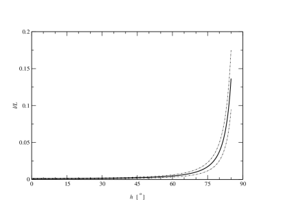
Figure 2: The ratio between the distances traveled by neutrinos in the Earth’s atmosphere and the Earth’s matter density profile $l/L$ as a function of the nadir angle $h$. The solid curve is plotted for $d=15\;{\rm km}$, whereas the two dashed-dotted curves are plotted for $d=10\;{\rm km}$ and $d=20\;{\rm km}$, respectively.

Since we are interested in the traveling paths of atmospheric neutrinos that are only a small fraction in the atmosphere, we will restrict ourselves to the cases when $l/L\lesssim 0.10$, which corresponds to a nadir angle

$$h=\arctan\sqrt{\frac{(1+2\frac{l}{L})^{2}-(1+\frac{d}{R_{\oplus}})^{2}}{(1+\frac{d}{R_{\oplus}})^{2}-1}}\lesssim 84^{\circ}.$$

In the limit $h\to 90^{\circ}$, the neutrinos travel the “maximal” distance in the atmosphere and just touch the surface of the Earth.

For two neutrino flavors we have the effective (vacuum) mixing parameters $\theta\simeq\theta_{13}\simeq 5^{\circ}$, which is below the CHOOZ upper bound and $\Delta m^{2}\simeq\Delta m_{32}^{2}\simeq 2.5\cdot 10^{-3}\;{\rm eV}^{2}$ [1], which is the latest best fit value of the Super-Kamiokande collaboration. Furthermore, we assume completely Earth-through-going atmospheric neutrinos ($h=0$) with neutrino energy $E_{\nu}=1\;{\rm GeV}$, which is a reasonable value of the neutrino energy for atmospheric neutrinos.

In Fig. 3, we show the relative error $\epsilon^{\prime}_{e\mu}$ of the transition probability for $\nu_{e}\leftrightarrow\nu_{\mu}$ that one makes omitting the Earth’s atmosphere in the calculation of the transition probability $P_{e\mu}$.

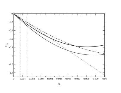
Figure 3: The relative error $\epsilon^{\prime}_{e\mu}$ as a function of the ratio $l/L$ for atmospheric neutrinos, different numbers of neutrino flavors, as well as different models of the matter density profile. For all curves we have used $E_{\nu}=1\;{\rm GeV}$ (reasonable for atmospheric neutrinos) and $h=0$ (completely Earth-through-going neutrinos). The dotted line: Eq. (22) with $\rho_{A}\simeq 7.8\;{\rm g/cm^{3}}$; the dashed curve: Eq. (LABEL:eq:e2) with $\rho_{A}\simeq 7.8\;{\rm g/cm^{3}}$; the thin solid curve: the Earth matter density profile with two neutrino flavors; the thick solid curve: the Earth matter density profile with three neutrino flavors. The two vertical dashed-dotted lines mark the interval relevant for the Earth’s atmosphere. The differences of the slopes of the curves close to $l/L=0$ are due to different models of the matter density profile.

The dotted line is a plot of Eq. (22), whereas the dashed curve is a plot of Eq. (LABEL:eq:e2). Both these plots assume a value of the matter density parameter $A$ that corresponds to the average value of the density of the Earth, i.e., $\rho_{A}\simeq 7.8\;{\rm g/cm^{3}}$. We note that Eq. (22) is a good approximation to Eq. (LABEL:eq:e2) for the values of $l/L$ that are relevant for the Earth’s atmosphere. The thin and thick solid curves use the usual mantle-core-mantle step function approximation for the Earth matter density profile. The thin solid curve is a plot using two neutrino flavors, whereas the thick solid curve is a plot using three neutrino flavors. We observe that the absolute value of the relative error $\epsilon^{\prime}_{e\mu}$ of the transition probability $P_{e\mu}$ is of the order of 15% - 25% depending on the value of the thickness of the atmosphere. This is a large error and shows that the atmosphere cannot be neglected in trustable analyses. Increasing the value of the vacuum mixing angle $\theta$ from $5^{\circ}$ to $10^{\circ}$, the relative error becomes even larger $\epsilon^{\prime}_{e\mu}\sim 50\%$. In order to separate the thickness effects of the thin density layer perturbation from the matter effects, we determine the relative error $\epsilon^{\prime}_{e\mu}$ for $A=0$, i.e., the relative error induced by the difference in the baseline lengths, to be

$$\epsilon^{\prime}_{e\mu}(L,l;0)=\frac{\sin^{2}x_{21}}{\sin^{2}X_{21}}+\sin 2x_{21}\cot X_{21}$$

$$-2\sin^{2}x_{21}\simeq 0.0304\approx 3\%$$ (25)

with $L=12742\;{\rm km}$ and $l=15\;{\rm km}$. Thus, the thickness effects are small compared with the matter effects. Note that the above formula is independent of the vacuum mixing angle $\theta$.

So far the present analysis for two neutrino flavors has been conducted on the level of transition probabilities using a monochromatic value of the neutrino energy $E_{\nu}$. In practice, however, the energy resolution of an experiment must be taken into account including energy uncertainties (or even better the analysis should be performed on the level of neutrino event rates), since neutrinos are neither produced nor detected with sharp energy. Another problem is attached to the definitions of the relative errors in Eqs. (LABEL:eq:e2) and (22). In the case when $P_{e\mu}(L,l;A)$ and/or $P_{e\mu}(L;A)$ become zero, the corresponding relative errors $\epsilon_{e\mu}$ and $\epsilon^{\prime}_{e\mu}$ go to infinity. Also when $P_{e\mu}(L,l;A)$ and $P_{e\mu}(L;A)$ are small, we will obtain large errors. This problem can be overcome by averaging over the neutrino energy, which will smoothen the transition probabilities and therefore lead to less varying errors. Thus, let us next estimate the relative error $\epsilon^{\prime}_{e\mu}$ when the resolution of the neutrino energy has been included. We assume for simplicity that the neutrinos are Gaussian distributed in energy with an average neutrino energy $\bar{E}_{\nu}$ and a corresponding uncertainty $\Delta E_{\nu}$. The Gaussian average is defined by

$$\langle\epsilon^{\prime}_{e\mu}\rangle=\frac{1}{\Delta E_{\nu}\sqrt{2\pi}}$$

$$\times\int_{-\infty}^{\infty}\epsilon^{\prime}_{e\mu}(E_{\nu})e^{-\frac{(E_{\nu}-\bar{E}_{\nu})^{2}}{2(\Delta E_{\nu})^{2}}}\,dE_{\nu}.$$ (26)

The energy resolution of the Super-Kamiokande experiment is of the order of magnitude $\Delta E_{\nu}\sim E_{\nu}$. Using this energy resolution and an average neutrino energy $\bar{E}_{\nu}=1\;{\rm GeV}$, we can, for example, compute the Gaussian averaged relative error $\langle\epsilon^{\prime}_{e\mu}\rangle$ for the case given in Eq. (25), and we obtain $\langle\epsilon^{\prime}_{e\mu}(L,l;0)\rangle\simeq 0.0181\approx 2\%$. Indeed, the Gaussian averaged relative error is smaller than the non-averaged one.

For three neutrino flavors the most probable vacuum mixing parameters are $\theta_{12}\simeq 45^{\circ}$, $\theta_{13}\simeq 5^{\circ}$, $\theta_{23}\simeq 45^{\circ}$, $\delta_{CP}=0$, $\Delta m_{21}^{2}\simeq 3.65\cdot 10^{-5}\;{\rm eV}^{2}$, and $\Delta m_{32}^{2}\simeq 2.5\cdot 10^{-3}\;{\rm eV}^{2}$. The values of the parameters $\theta_{12}$ and $\Delta m_{21}^{2}$ correspond to the best fit point values of the large mixing angle (LMA) solution [13], whereas the values of the parameters $\theta_{23}$ and $\Delta m_{32}^{2}$ correspond to the latest best fit values from the Super-Kamiokande collaboration [1]. Using these values of the mixing parameters, we have in Figs. 4 - 6 plotted as density plots the absolute errors of the transition probabilities for $\nu_{e}\leftrightarrow\nu_{\mu}$, $\nu_{e}\leftrightarrow\nu_{\tau}$, and $\nu_{\mu}\leftrightarrow\nu_{\tau}$. These density plots also use the mantle-core-mantle step function approximation for the Earth’s matter density profile. We observe that the errors are largest for $P_{\mu\tau}$ and smallest for $P_{e\mu}$. Actually, for $P_{\mu\tau}$ the error can be close to 100% depending on the nadir angle and the neutrino energy. The errors decrease for increasing neutrino energy and naturally they increase for increasing nadir angle. Furthermore, note that the errors are due to both the difference in lengths of the baselines ($L^{\prime}=L+l$ for the case with the Earth’s matter density profile included; $L$ for the case without) as well as the difference in density $\Delta\rho=\rho_{A}$, i.e., the errors are thickness and matter effects arising from the thin density layer perturbation.

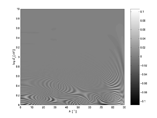
Figure 4: The difference $\Delta P_{e\mu}$ as a function of the nadir angle $h$ and the neutrino energy $E_{\nu}$ for three neutrino flavors assuming the Earth’s matter density profile.

Figure 5: The difference $\Delta P_{e\tau}$ as a function of the nadir angle $h$ and the neutrino energy $E_{\nu}$ for three neutrino flavors assuming the Earth’s matter density profile.

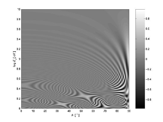
Figure 6: The difference $\Delta P_{\mu\tau}$ as a function of the nadir angle $h$ and the neutrino energy $E_{\nu}$ for three neutrino flavors assuming the Earth’s matter density profile.

4 Summary and conclusions

In summary, we have derived analytically exact as well as approximate formulas for the absolute and relative errors of the transition probabilities for neutrino oscillations using a thin density layer perturbation in the case of two neutrino flavors. It should be noted that for three neutrino flavors this is not easily achieved. However, for three neutrino flavors we have studied the influence of a thin density layer perturbation numerically. The studies were carried out for one of the most interesting experimental setups, i.e., atmospheric neutrinos. We assumed the Earth’s matter density profile with the Earth’s atmosphere as the thin density layer perturbation.

In conclusion, we found that the transition probabilities are rather influenced by a thin density layer perturbation, even though its length is at least one order of magnitude smaller than that of the matter density profile. In the case of atmospheric neutrinos, using three neutrino flavors, the absolute error $\Delta P_{\mu\tau}$ of the transition probability $P_{\mu\tau}$ could nearly be as large as 100% for certain realistic nadir angles and neutrino energies. This is despite the fact that the distance traveled by neutrinos in the Earth’s atmosphere is much shorter than the distance that they travel in the Earth’s matter density profile; at least for nadir angles $h\lesssim 84^{\circ}$. Thus, it is important also to include the Earth’s atmosphere in the analyses of atmospheric neutrinos. Note that we are fully aware of that in most such analyses this is certainly done. Furthermore, taking energy resolution into account will definitely reduce the errors of the transition probabilities. The purpose of this work was to investigate and determine the actual effects of the Earth’s atmosphere being in principle just a thin density layer perturbation in comparison with the Earth’s matter density profile itself.

Finally, note that this paper is in principle the “counterpart” to the study performed in Ref. [14], in which the distance traveled by neutrinos in matter is assumed to be short compared with the distance in vacuum.

References

- [1] Super-Kamiokande Collaboration, T. Toshito, hep-ex/0105023.
- [2] SNO Collaboration, Q.R. Ahmad et al., Phys. Rev. Lett. 87 (2001) 071301, nucl-ex/0106015.
- [3] T. Ohlsson and H. Snellman, Phys. Lett. B 474 (2000) 153, hep-ph/9912295, 480 (2000) 419(E).
- [4] S.T. Petcov, Phys. Lett. B 434 (1998) 321, hep-ph/9805262, 444 (1998) 584(E).
- [5] E.K. Akhmedov, Nucl. Phys. B 538 (1999) 25, hep-ph/9805272.
- [6] M.V. Chizhov and S.T. Petcov, Phys. Rev. D 63 (2001) 073003, hep-ph/9903424.
- [7] T. Ohlsson and H. Snellman, J. Math. Phys. 41 (2000) 2768, hep-ph/9910546, 42 (2001) 2345(E).
- [8] P.M. Fishbane and P. Kaus, Phys. Lett. B 506 (2001) 275, hep-ph/0012088.
- [9] E. Akhmedov et al., Nucl. Phys. B 608 (2001) 394, hep-ph/0105029.
- [10] CHOOZ Collaboration, M. Apollonio et al., Phys. Lett. B 420 (1998) 397, hep-ex/9711002.
- [11] CHOOZ Collaboration, M. Apollonio et al., Phys. Lett. B 466 (1999) 415, hep-ex/9907037.
- [12] M. Freund and T. Ohlsson, Mod. Phys. Lett. A 15 (2000) 867, hep-ph/9909501, and references therein.
- [13] M.C. Gonzalez-Garcia, C. Peña-Garay and A.Y. Smirnov, Phys. Rev. D 63 (2001) 113004, hep-ph/0012313.
- [14] E.K. Akhmedov, Phys. Lett. B 503 (2001) 133, hep-ph/0011136.