hep-ph/0108273

The structure of large logarithmic corrections
at small transverse momentum
in hadronic collisions

Daniel de Florian${}^{\,a,d}$   and   Massimiliano Grazzini${}^{\,b,c,d}$

${}^{a}\,$Departamento de Física, FCEYN, Universidad de Buenos Aires, (1428) Pabellón 1 Ciudad Universitaria, Capital Federal, Argentina

${}^{b}\,$Dipartimento di Fisica, Università di Firenze, I-50125 Florence, Italy

${}^{c}\,$INFN, Sezione di Firenze, I-50125 Florence, Italy

${}^{d}\,$Institute for Theoretical Physics, ETH-Hönggerberg, CH 8093 Zürich, Switzerland

Abstract

We consider the region of small transverse momenta in the production of high-mass systems in hadronic collisions. By using the current knowledge on the infrared behaviour of tree-level and one-loop QCD amplitudes at ${\cal O}(\alpha_{\mathrm{S}}^{2})$, we analytically compute the general form of the logarithmically-enhanced contributions up to next-to-next-to-leading logarithmic accuracy. By comparing the results with $q_{T}$-resummation formulae we extract the coefficients that control the resummation of the large logarithmic contributions for both quark and gluon channels. Our results show that within the conventional resummation formalism the Sudakov form factor is actually process-dependent.

hep-ph/0108273

August 2001

1 Introduction

The transverse-momentum distribution of systems with high invariant mass produced in high-energy hadron collisions is important for QCD studies and for physics studies beyond the Standard Model (see, e.g., Refs. [1]–[4]).

We consider the inclusive hard-scattering process

$$h_{1}(p_{1})+h_{2}(p_{2})\rightarrow F(Q^{2},q_{T}^{2};\phi)+X\;\;,$$ (1)

where the final-state system $F$ is produced by the collision of the two hadrons $h_{1}$ and $h_{2}$ with momenta $p_{1}$ and $p_{2}$, respectively. The final state $F$ is a generic system of non-strongly interacting particles, such as one or more vector bosons $(\gamma^{*},W,Z,\dots)$, Higgs particles ($H$) and so forth. We denote by $\sqrt{s}$ the center-of-mass energy of the colliding hadrons $(s=(p_{1}+p_{2})^{2}\simeq 2p_{1}p_{2})$, and by $Q^{2}$ and $q_{T}^{2}$ the invariant mass and total transverse momentum of the system $F$, respectively. The additional variable $\phi$ in (1) denotes the possible dependence on the kinematics of the final state particles in $F$ (such as rapidities, individual transverse momenta and so forth).

We assume that at the parton level the system $F$ is produced with vanishing $q_{T}$ (i.e. with no accompanying final-state radiation) in the leading-order (LO) approximation. Since $F$ is colourless, the LO partonic subprocess is either $q_{f}\bar{q}_{f^{\prime}}$ annihilation, as in the case of $\gamma^{*},W$ and $Z$ production, or $gg$ fusion, as in the case of the production of a Higgs boson $H$.

When the transverse momentum of the produced system $q_{T}^{2}$ is of the order of its invariant mass $Q^{2}$ the fixed order calculation is reliable. In the region $q_{T}^{2}\ll Q^{2}$ large logarithmic corrections of the form $\alpha_{\mathrm{S}}^{n}/q_{T}^{2}\log^{2n-1}Q^{2}/q_{T}^{2}$ appear, which spoil the convergence of fixed-order perturbative calculations. The logarithmically-enhanced terms have to be evaluated at higher perturbative orders, and possibly resummed to all orders in the QCD coupling constant $\alpha_{\mathrm{S}}$. The all-order resummation formalism was developed in the eighties [5]–[14]. The structure of the resummed distribution is given in terms of a transverse-momentum form factor and of process-dependent contributions.

The coefficients that control the resummation of the large logarithmic contributions for a given process in (1) can be computed at a given order if an analytic calculation at large $q_{T}$ at the same order exists. At first order in $\alpha_{\mathrm{S}}$ the structure of the large logarithmic contributions is known to be universal and depends only on the channel in which the system is produced in the LO approximation. At second relative order in $\alpha_{\mathrm{S}}$, only a few analytical calculations are available, like the pioneering one for lepton-pair Drell–Yan production, performed by Ellis, Martinelli and Petronzio in Ref. [15]. Using the results of Ref. [15] Davies and Stirling [14] (see also [16]) were able to obtain the complete structure of the ${\cal O}(\alpha_{\mathrm{S}}^{2})$ logarithmic corrections for that process.

The analysis performed by Davies and Stirling is by far non trivial because it requires the integration of the analytic $q_{T}$ distribution in the small $q_{T}$ limit. Moreover the calculation cannot tell anything about the dependence of these coefficients on the particular process in (1) and should in principle be repeated for each process.

In this paper we address this problem with a completely independent and general method. Our basic observation is that the large logarithmic corrections are of infrared (soft and collinear) nature, and thus their form can be predicted once and for all in a general (process independent) manner.

The structure of the logarithmically-enhanced contributions at ${\cal O}(\alpha_{\mathrm{S}}^{n})$ is controlled by the infrared limit of the relevant QCD amplitudes at the same order. The infrared behaviour of QCD amplitudes at ${\cal O}(\alpha_{\mathrm{S}})$ is known since long time [17]. Recently, soft and collinear singularities arising in tree-level [18, 19] and one-loop [20, 21, 22, 23] QCD amplitudes at ${\cal O}(\alpha_{\mathrm{S}}^{2})$ have been extensively studied and the corresponding kernels have been computed [18]-[25]. By using this knowledge, and exploiting the relatively simple kinematics of the process (1), we will construct general approximations of the relevant QCD matrix elements that are able to control all singular regions corresponding to $q_{T}\rightarrow 0$ avoiding double counting. By using these approximations we will compute the general structure of the ${\cal O}(\alpha_{\mathrm{S}}^{2})$-logarithmically-enhanced contributions both for ${\bar{q}}q$- and for $gg$-initiated processes.

The results provide an important check of the validity of the resummation formalism and allow to extract the general form of the resummation coefficients. In particular in the quark channel we can confirm the results of Ref. [14] in the case of Drell–Yan and in the gluon channel we can give the coefficients in the important case of Higgs boson production through gluon-gluon fusion.

The universality of our method relies on the fact that the infrared factorization formulae we use depend only on the channel ($q{\bar{q}}$ or $gg$) in which the system $F$ is produced at LO and not on the details of $F$.

Our main results were anticipated in a short letter [26]. This paper is organized as follows. In section 2 we review the framework of the resummation formalism and present the strategy for the calculation. In section 3 we perform the calculation explicitly for the ${\cal O}(\alpha_{\mathrm{S}})$ corrections and extract the first order coefficients. Section 4 and 5 are devoted to the calculation at ${\cal O}(\alpha_{\mathrm{S}}^{2})$ for the quark and the gluon channel and constitute the main part of this work. Finally in section 6 we present our final results and discussion.

2 Resummation formula

The transverse momentum distribution for the process in Eq. (1) can be written as:

$$\frac{d\sigma_{F}}{dQ^{2}\;dq_{T}^{2}\;d\phi}=\left[\frac{d\sigma_{F}}{dQ^{2}\;dq_{T}^{2}\;d\phi}\right]_{{\rm res.}}+\left[\frac{d\sigma_{F}}{dQ^{2}\;dq_{T}^{2}\;d\phi}\right]_{{\rm fin.}}\;\;.$$ (2)

Both terms on the right-hand side are obtained as convolutions of partonic cross sections and the parton distributions $f_{a/h}(x,Q^{2})$ ($a=q_{f},{\bar{q}}_{f},g$ is the parton label) of the colliding hadrons.

The partonic cross section that enters in the resummed part (the first term on the right-hand side) contains all the logarithmically-enhanced contributions $\alpha_{\mathrm{S}}^{n}/q_{T}^{2}\log^{m}Q^{2}/q_{T}^{2}$. Thus, this part has to be evaluated by resumming the logarithmic terms to all orders in perturbation theory. On the contrary, the partonic cross section in the second term on the right-hand side is finite (or at least integrable) order-by-order in perturbation theory when $q_{T}\rightarrow 0$. It can thus be computed by truncating the perturbative expansion at a given fixed order in $\alpha_{\mathrm{S}}$.

Since in the following we are interested in the small-$q_{T}$ limit we will be concerned only with the first term in Eq. (2). The resummed component is

$$\left[\frac{Q^{2}\,d\sigma_{F}}{dQ^{2}\;dq_{T}^{2}\,d\phi}\right]_{{\rm res.}}= \sum_{a,b}\int_{0}^{1}dx_{1}\int_{0}^{1}dx_{2}\int_{0}^{\infty}db\;\frac{b}{2}\;J_{0}(bq_{T})\;f_{a/h_{1}}(x_{1},b_{0}^{2}/b^{2})\;f_{b/h_{2}}(x_{2},b_{0}^{2}/b^{2})$$

$$\cdot\, s\,W_{ab}^{F}(x_{1}x_{2}s;Q,b,\phi)\;\;.$$ (3)

The Bessel function $J_{0}(bq_{T})$ and the coefficient $b_{0}=2e^{-\gamma_{E}}$ ($\gamma_{E}=0.5772\dots$ is the Euler number) have a kinematical origin. To correctly take into account the kinematics constraint of transverse-momentum conservation, the resummation procedure has to be carried out in the impact-parameter $b$-space. The resummed coefficient $W_{ab}^{F}$ is

$$W_{ab}^{F}(s;Q,b,\phi) =\sum_{c}\int_{0}^{1}dz_{1}\int_{0}^{1}dz_{2}\;C_{ca}^{F}(\alpha_{\mathrm{S}}(b_{0}^{2}/b^{2}),z_{1})\;C_{{\bar{c}}b}^{F}(\alpha_{\mathrm{S}}(b_{0}^{2}/b^{2}),z_{2})\;\delta(Q^{2}-z_{1}z_{2}s)$$

$$\cdot\,\frac{d\sigma_{c{\bar{c}}}^{(LO)\,F}}{d\phi}\;S_{c}^{F}(Q,b)\;\;.$$ (4)

where $d\sigma_{c\bar{c}}^{(LO)}/d\phi$ corresponds to the leading order cross section for the production of the large invariant mass system $F$ in the $c{\bar{c}}$ channel, with $c$ representing either a quark $q$ or a gluon $g$. The resummation of the large logarithmic corrections is achieved by exponentiation, that is by showing that the Sudakov form factor can be expressed as

$$S_{c}(Q,b)=\exp\left\{-\int_{b_{0}^{2}/b^{2}}^{Q^{2}}\frac{dq^{2}}{q^{2}}\left[A_{c}(\alpha_{\mathrm{S}}(q^{2}))\;\log\frac{Q^{2}}{q^{2}}+B_{c}(\alpha_{\mathrm{S}}(q^{2}))\right]\right\}\,.$$ (5)

The functions $A_{c}(\alpha_{\mathrm{S}})$, $B_{c}(\alpha_{\mathrm{S}})$, as well as the coefficient functions $C_{ab}(\alpha_{\mathrm{S}},z)$ in Eqs. (2,5) are free of large logarithmic corrections and have perturbative expansions in $\alpha_{\mathrm{S}}$ as

$$A_{c}(\alpha_{\mathrm{S}}) = \sum_{n=1}^{\infty}\left(\frac{\alpha_{\mathrm{S}}}{2\pi}\right)^{n}A_{c}^{(n)}\;\;,$$ (6)

$$B_{c}(\alpha_{\mathrm{S}}) = \sum_{n=1}^{\infty}\left(\frac{\alpha_{\mathrm{S}}}{2\pi}\right)^{n}B_{c}^{(n)}\;\;,$$ (7)

$$C_{ab}(\alpha_{\mathrm{S}},z) = \delta_{ab}\,\delta(1-z)+\sum_{n=1}^{\infty}\left(\frac{\alpha_{\mathrm{S}}}{2\pi}\right)^{n}C_{ab}^{(n)}(z)\;\;.$$ (8)

The coefficients of the perturbative expansions $A_{c}^{(n)}$, $B_{c}^{(n)}$ and $C_{ab}^{(n)}(z)$ are the key of the resummation procedure since their knowledge allows to perform the resummation to a given Logarithmic order: $A^{(1)}$ leads to the resummation of leading logarithmic (LL) contributions, $\{A^{(2)},B^{(1)},C^{(1)}\}$ give the next-to-leading logarithmic (NLL) terms, $\{A^{(3)},B^{(2)},C^{(2)}\}$ give the next-to-next-to-leading logarithmic (NNLL) terms, and so forth. The coefficient functions $C_{ab}^{(n)}(z)$ depend on the process, as it has been confirmed by calculations of $C_{ab}^{(1)}(z)$ for several processes. The Sudakov form factor $S_{c}(Q,b)$ that enters Eq. (2) is often supposed to be universal. However, as we will show, this is not the case, and anticipating our results we label all process-dependent coefficients by the upper index $F$. The coefficients $A^{(1)}$, $B^{(1)}$, $A^{(2)}$ are universal and are known both for the quark [10] and for the gluon [13] form factors

$$A_{q}^{(1)}=2C_{F}\;\;,\quad\quad\;\;A_{g}^{(1)}=2C_{A}\;,$$

$$B_{q}^{(1)}=-3C_{F}\;\;,\quad B_{g}^{(1)}=-2\beta_{0}\;,$$ (9)

$$A_{q}^{(2)}=2C_{F}K\;\;,\quad A_{g}^{(2)}=2C_{A}K\;,$$

where

$$\beta_{0}=\frac{11}{6}C_{A}-\frac{2}{3}\,n_{f}T_{R}$$ (10)

and

$$K=\left(\frac{67}{18}-\frac{\pi^{2}}{6}\right)C_{A}-\frac{10}{9}\,n_{f}T_{R}\;\;.$$ (11)

The NNLL coefficient $B^{(2)}$ was computed by Davies and Stirling [14] for the case of Drell–Yan (DY):

$$B_{q}^{(2)DY}=C_{F}^{2}\left(\pi^{2}-\frac{3}{4}-12\zeta(3)\right)+C_{F}\,C_{A}\left(\frac{11}{9}\pi^{2}-\frac{193}{12}+6\zeta(3)\right)+C_{F}\,n_{f}\,T_{R}\left(\frac{17}{3}-\frac{4}{9}\pi^{2}\right)\,,$$ (12)

where $\zeta(n)$ is the Riemann $\zeta$-function $(\zeta(3)=1.202\dots)$. It is also worth noticing that, even though there is no analytical result available for it, the coefficient $A_{q,g}^{(3)}$ has been extracted numerically with a very good precision in Ref. [29].

As anticipated in the introduction, a direct way to obtain the coefficients in Eqs. (6-7) at a given order involves the computation of the differential cross section ${d\sigma}/{dq_{T}^{2}dQ^{2}d\phi}$ at small $q_{T}$ at the same order. A comparison with the power expansion in $\alpha_{\mathrm{S}}$ of the resummed result in Eq. (2) allows to extract the coefficients that control the resummation of the large logarithmic terms. However, it has been shown by Davies and Stirling that is it more convenient to take $z=Q^{2}/s$ moments of the differential cross section defining the dimensionless quantity

$$\Sigma(N)=\int_{0}^{1-2q_{T}/Q}dz\,z^{N}\frac{Q^{2}q_{T}^{2}}{d\sigma_{0}/d\phi}\frac{d\sigma}{dq_{T}^{2}dQ^{2}d\phi}\,.$$ (13)

Notice that in the definition of $\Sigma$ the cross section has been normalized with respect to the lowest order partonic contribution ${d\sigma_{0}/d\phi}$ and multiplied by $q_{T}^{2}$ to cancel its $1/q_{T}^{2}$ singular behaviour in the limit $q_{T}\rightarrow 0$. The upper limit of integration $z=1-2q_{T}/Q(\sqrt{1+q_{T}^{2}/Q^{2}}-q_{T}/Q)\sim 1-2q_{T}/Q$ has been approximated to a first order expansion in $q_{T}/Q$ and corresponds to the kinematics for the emission of soft particles (i.e, when the center of mass energy $s$ is just enough to produce the system with invariant mass $Q$ and transverse momentum $q_{T}$). Working with moments allows to avoid complicated convolution integrals implicit in (2) and makes possible to factorize the parton densities from the partonic contribution to the cross section. In this way, the corresponding expression from the resummed formula (2) reads

$$\Sigma(N)=\sum_{i,j}f_{i/h_{1}}(N,\mu^{2}_{F})f_{j/h_{2}}(N,\mu^{2}_{F})\,\Sigma_{ij}(N)$$ (14)

where

$$\Sigma_{ij}(N)=\sum_{a,b}\int_{0}^{\infty}b\,db\frac{q_{T}^{2}}{2}\,J_{0}(bq_{T})\,{C}^{{F}}_{ca}\left(N,\alpha_{\mathrm{S}}\left({b_{0}^{2}}/{b^{2}}\right)\right){C}^{{F}}_{\overline{c}b}\left(N,\alpha_{\mathrm{S}}\left({b_{0}^{2}}/{b^{2}}\right)\right)$$

$$\cdot\exp\Bigg{\{}\!-\int_{b_{0}^{2}/b^{2}}^{Q^{2}}\frac{dq^{2}}{q^{2}}\left[{A}_{c}(\alpha_{\mathrm{S}}(q^{2}))\;\log\frac{Q^{2}}{q^{2}}+{B}_{c}^{{F}}(\alpha_{\mathrm{S}}(q^{2}))\right]-\!\int_{{b_{0}^{2}}/{b^{2}}}^{\mu^{2}_{F}}\frac{dq^{2}}{q^{2}}\,\left(\gamma_{ai}+\gamma_{bj}\right)(N,\alpha_{\mathrm{S}}(q^{2}))\Bigg{\}}$$

and an ordered exponential is understood. Notice that the appearance of an extra term involving the anomalous dimensions $\gamma_{ab}$ in the exponential in (2) is due to the evolution of the parton densities from the original scale $b_{0}^{2}/b^{2}$ in (2) to the arbitrary factorization scale $\mu_{F}$ at which they are now evaluated.

In order to extract the resummation coefficients, we can directly study the partonic contribution $\Sigma_{ij}$. Furthermore, since we want to perform a calculation of $\Sigma_{ij}$ to ${\cal O}(\alpha_{\mathrm{S}}^{2})$  and our main interest is the second order coefficient $B^{(2)}$, it is clear that only the diagonal contribution $\Sigma_{c{\bar{c}}}$ can give the desired information. Each possible “flavour changing” contribution in Eq. (2) would add at least one extra power of $\alpha_{\mathrm{S}}$ in the perturbative expansion. ‘Non-diagonal’ contributions to $\Sigma_{ij}$, which can be evaluated in a simpler way, might be used to check the structure and consistency of the resummation framework at a given perturbative order but do not provide any additional information on the coefficients.

In order to have transverse momentum $q_{T}\neq 0$ at least one gluon has to be emitted and, therefore, the perturbative expansion of $\Sigma_{c\overline{c}}$ begins at ${\cal O}(\alpha_{\mathrm{S}})$

$$\Sigma_{c\overline{c}}(N)=\frac{\alpha_{\mathrm{S}}}{2\pi}\;\Sigma^{(1)}_{c\overline{c}}(N)+\left(\frac{\alpha_{\mathrm{S}}}{2\pi}\right)^{2}\Sigma^{(2)}_{c\overline{c}}(N)+\cdots\,.$$ (16)

From the expansion of the resummed formula (2) it is possible to obtain the expression for the first two coefficients in (16) as

$$\Sigma_{c{\bar{c}}}^{(1)}(N)={A}_{c}^{(1)}\log\frac{Q^{2}}{q_{T}^{2}}+{B}_{c}^{(1)}+2\gamma_{cc}^{(1)}(N)$$ (17)

and

$${\Sigma^{(2)}_{c\bar{c}}}{(N)}=\log^{3}\frac{Q^{2}}{q_{T}^{2}}\left[-\frac{1}{2}\left({A}_{c}^{(1)}\right)^{2}\right]$$

$$+\log^{2}\frac{Q^{2}}{q_{T}^{2}}\left[-\frac{3}{2}\left({B}_{c}^{(1)}+2\gamma_{cc}^{(1)}(N)\right){A}_{c}^{(1)}+\beta_{0}{A}_{c}^{(1)}\right]$$

$$+\log\frac{Q^{2}}{q_{T}^{2}}\left[{A}_{c}^{(2)}+\beta_{0}\left({B}_{c}^{(1)}+2\gamma_{cc}^{(1)}(N)\right)-\left({B}_{c}^{(1)}+2\gamma_{cc}^{(1)}(N)\right)^{2}\right.$$

$$\hskip 34.14322pt\left.+2{A}_{c}^{(1)}{C}_{cc}^{(1){F}}(N)-2\sum_{j\neq c}\gamma_{cj}^{(1)}(N)\gamma_{jc}^{(1)}(N)\right]$$

$$+{B}_{c}^{(2){F}}+2\gamma_{cc}^{(2)}(N)+2\left({B}_{c}^{(1)}+2\gamma_{cc}^{(1)}(N)\right){C}_{cc}^{(1){F}}(N)+2\zeta(3)({A}_{c}^{(1)})^{2}$$

$$-{2\beta_{0}}{C}_{cc}^{(1){F}}(N)+2\sum_{j\neq c}\left[{C}_{cj}^{(1){F}}(N)\gamma_{jc}^{(1)}(N)\right]\,.$$ (18)

The computation of $\Sigma_{c{\bar{c}}}^{(1)}(N)$ can provide information on the first order coefficients ${A}_{c}^{(1)}$ (the logarithmic term in (17)) and ${B}_{c}^{(1)}$ (the constant term in (17)) as well as on the one-loop anomalous dimensions $\gamma_{cc}^{(1)}(N)$ ( the $N-$dependent term in (17).). In the same way, the coefficients ${A}_{c}^{(2)}$ and ${B}_{c}^{(2){F}}$ can be extracted from the second order result (2). At this order, also the coefficient functions ${C}_{ij}^{(1){F}}(N)$ contribute to the logarithmic and constant terms and therefore should be known in order to be able to proceed with the extraction of ${A}_{c}^{(2)}$ and ${B}_{c}^{(2){F}}$ . Fortunately, there is another related quantity which allows to obtain the coefficient functions ${C}_{ij}^{(1){F}}(N)$ from a first order calculation. This is the $q_{T}$-integrated cross section

$$\int_{0}^{p_{T}^{2}}\frac{dq_{T}^{2}}{q_{T}^{2}}\Sigma_{i\overline{c}}\,.$$ (19)

When $p_{T}^{2}\ll Q^{2}$ the perturbative expansion to ${\cal O}(\alpha_{\mathrm{S}})$ reads (neglecting again terms that vanish when $p_{T}\rightarrow 0$)

$$\int_{0}^{p_{T}^{2}}\frac{dq_{T}^{2}}{q_{T}^{2}}\Sigma_{c\overline{c}} =\frac{\alpha_{\mathrm{S}}}{2\pi}\left[-\frac{1}{2}{A}_{c}^{(1)}\log^{2}\frac{Q^{2}}{p_{T}^{2}}-({B}_{c}^{(1)}+2\gamma_{cc}^{(1)}(N))\log\frac{Q^{2}}{p_{T}^{2}}+2{C}_{cc}^{(1){F}}(N)\right]$$

$$\int_{0}^{p_{T}^{2}}\frac{dq_{T}^{2}}{q_{T}^{2}}\Sigma_{i\overline{c}} =\frac{\alpha_{\mathrm{S}}}{2\pi}\left[-\gamma_{ci}^{(1)}(N)\log\frac{Q^{2}}{p_{T}^{2}}+{C}_{ci}^{(1){F}}(N)\right]~{}~{}~{}~{}~{}~{}~{}~{}~{}~{}~{}~{}~{}~{}~{}~{}~{}~{}i\neq c\,.$$ (20)

The integration over $q_{T}$ adds one power in the logarithm, with the coefficient functions ${C}_{ij}^{(1){F}}(N)$ appearing now in the constant term. It is worth noticing that at variance with the calculation of $\Sigma$ the configuration with $q_{T}=0$ now contributes to Eq. (19).

In the quark channel $(c=q)$, for the sake of simplicity and in order to compare directly with the calculation performed in [14], we will concentrate on the non-singlet contribution to the cross section defined by

$$\sigma^{\rm NS}=\sum_{ff^{\prime}}\left(\sigma_{q_{f}\bar{q}_{f^{\prime}}}-\sigma_{q_{f}q_{f^{\prime}}}\right)\,.$$ (21)

The second order expansion for $\Sigma_{q\overline{q}}^{\rm NS}(N)$ in terms of the resummation coefficients reads like the one in Eq. (2) but without the ‘singlet’ contributions involving $\sum_{j\neq c}$ and with the corresponding non-singlet anomalous dimension. In the following the label NS will be always understood in $\Sigma_{q{\bar{q}}}$.

3 The calculation at ${\cal O}(\alpha_{\mathrm{S}})$

The calculation at ${\cal O}(\alpha_{\mathrm{S}})$ is not difficult and the results are rather well known. Nevertheless, we will give in this section the details on the computation as a way to present the main ideas of the method developed to obtain the resummation coefficients.

At this order only one extra gluon of momentum $k$ can be radiated and the kinematics for the process $c\bar{c}\rightarrow g+F$ is (see Fig. 1)

$$p_{1}+p_{2}\rightarrow k+q\,.$$ (22)

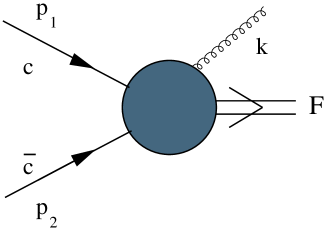
Figure 1: ${\cal O}(\alpha_{\mathrm{S}})$ contribution to the process (1)

We denote the corresponding matrix element by ${\cal M}^{(0)}_{c\bar{c}\rightarrow g\,F}\left(p_{1},p_{2},k,\phi\right)$ and the usual invariants are defined as

$$s=(p_{1}+p_{2})^{2}~{}~{}~{}~{}u=(p_{2}-k)^{2}~{}~{}~{}~{}t=(p_{1}-k)^{2}~{}~{}~{}~{}z=Q^{2}/s\,.$$ (23)

The differential cross section can be written as

$$\frac{d\sigma_{c{\bar{c}}\rightarrow g\,F}}{dq_{T}^{2}dQ^{2}d\phi}=\int\frac{|{\cal M}^{(0)}_{c\bar{c}\rightarrow g\,F}\left(p_{1},p_{2},k,\phi\right)|^{2}}{8s(2\pi)^{2}}\frac{(4\pi)^{\epsilon}q_{T}^{-2\epsilon}}{\Gamma(1-\epsilon)}\,\frac{du}{u}\,\delta\left(\frac{1}{u}(u-u_{max})(u-u_{min})\right)\,,$$ (24)

where the two roots of the equation $(p_{1}+p_{2}-q)^{2}=0$ are given by

$$u_{min}=Q^{2}\;\frac{z-1-\sqrt{(1-z)^{2}-4z\,q_{T}^{2}/Q^{2}}}{2z}~{}~{}~{}~{}~{}~{}~{}~{}~{}u_{max}=Q^{2}\;\frac{z-1+\sqrt{(1-z)^{2}-4z\,q_{T}^{2}/Q^{2}}}{2z}\,.$$ (25)

In order to regularize both ultraviolet and infrared divergences we work in the conventional dimensional regularization scheme (CDR) with $4-2\epsilon$ space-time dimensions, considering two helicity states for massless quarks and $2-2\epsilon$ helicity states for gluons. The lowest-order cross section (at $q_{T}=0$) needed to construct $\Sigma$ in Eq. (13) is given by

$$\frac{d\sigma_{0}}{d\phi}=\frac{|{\cal M}_{c{\bar{c}}\rightarrow F}^{(0)}\left(p_{1},p_{2},\phi\right)|^{2}}{2s}\,,$$ (26)

in terms of the Born matrix element $|{\cal M}_{c{\bar{c}}\rightarrow F}^{(0)}\left(p_{1},p_{2},\phi\right)|^{2}$.

As has been stated, we want to obtain $\Sigma^{(1)}_{c{\bar{c}}}$ by using our knowledge on the behaviour of QCD matrix elements in the soft and collinear regions at ${\cal O}(\alpha_{\mathrm{S}})$. The starting point is the observation that, when $q_{T}^{2}$ is small, the additional gluon is constrained to be either collinear to one of the incoming partons or soft. Thus there are three singular regions of ${\cal M}^{(0)}_{c{\bar{c}}\rightarrow F}\left(p_{1},p_{2},k,\phi\right)$ in the $q_{T}\rightarrow 0$ limit:

• first collinear region: $p_{1}k\rightarrow 0$

• second collinear region: $p_{2}k\rightarrow 0$

• soft region: $k\rightarrow 0$.

It is clear that, since $q_{T}^{2}$ is small but does not vanish, these regions do not produce any real singularity, i.e. poles in $\epsilon$, but are responsible for the appearance of the logarithmically-enhanced contributions. When $p_{1}k\rightarrow 0$ the matrix element squared factorizes as follows:

$$|{\cal M}^{(0)}_{c{\bar{c}}\rightarrow g\,F}\left(p_{1},p_{2},k,\phi\right)|^{2}\simeq\frac{4\pi\alpha_{\mathrm{S}}\mu^{2\epsilon}}{z_{1}p_{1}k}{\hat{P}}_{cc}(z_{1},\epsilon)|{\cal M}^{(0)}_{c{\bar{c}}\rightarrow F}\left(z_{1}\,p_{1},p_{2},\phi\right)|^{2}\,,$$ (27)

where

$${\hat{P}}_{qq}(z,\epsilon) =C_{F}\left[\frac{1+z^{2}}{1-z}-\epsilon(1-z)\right]$$ (28)

$$\hat{P}_{gg}(z,\epsilon) =2C_{A}\left[\frac{z}{1-z}+\frac{1-z}{z}+z(1-z)\right]$$ (29)

are the $\epsilon$-dependent real Altarelli–Parisi (AP) kernels in the CDR scheme. In the left hand side of Eq. (27) the matrix element squared is obtained replacing the two collinear partons $c$ and $g$ by a parton $c$ with momentum $z_{1}p_{1}$.

Notice that in the gluon channel there are additional spin-correlated contributions and Eq. (27) is strictly valid only after azimuthal integration. Since here and in the following we will always be interested in azimuthal integrated quantities, Eq. (27) can be safely used also in the gluon channel.

In the limit $p_{2}k\rightarrow 0$ the singular behaviour is instead

$$|{\cal M}^{(0)}_{c{\bar{c}}\rightarrow g\,F}\left(p_{1},p_{2},k,\phi\right)|^{2}\simeq\frac{4\pi\alpha_{\mathrm{S}}\mu^{2\epsilon}}{z_{2}p_{2}k}{\hat{P}}_{cc}(z_{2},\epsilon)|{\cal M}^{(0)}_{c{\bar{c}}\rightarrow F}\left(p_{1},z_{2}\,p_{2},\phi\right)|^{2}\,.$$ (30)

Let us now consider the limit in which the gluon becomes soft. As it is well known soft-factorization formulae usually involve colour correlations, that make colour and kinematics entangled. In general colour correlations relate each pair of hard momentum partons in the Born matrix element. In this case the hard momentum partons are only two and colour conservation can be exploited to obtain:

$$|{\cal M}^{(0)}_{c{\bar{c}}\rightarrow g\,F}\left(p_{1},p_{2},k,\phi\right)|^{2}\simeq 4\pi\alpha_{\mathrm{S}}\mu^{2\epsilon}\;C_{c}\,4\,{\cal S}_{12}(k)|{\cal M}^{(0)}_{c{\bar{c}}\rightarrow F}\left(p_{1},p_{2},\phi\right)|^{2}\,,$$ (31)

where

$${\cal S}_{12}(k)=\frac{p_{1}p_{2}}{2p_{1}k\,p_{2}k}$$ (32)

is the usual eikonal factor and we have defined

$$C_{q}=C_{F}~{}~{}~{}~{}~{}~{}~{}~{}C_{g}=C_{A}\,.$$ (33)

In Eq. (31) colour correlations are absent and factorization is exact. This feature will persist also at ${\cal O}(\alpha_{\mathrm{S}}^{2})$.

In each of the singular regions discussed above, Eqs. (27), (30) and (31) provide an approximation of the exact matrix element that can be used to compute the cross section in the small $q_{T}$ limit. In principle it might be possible to split the phase space integration in regions where only soft or collinear configurations can arise, and use in each region the corresponding approximation. Unfortunately, such method probes to be very difficult to be extended to ${\cal O}(\alpha_{\mathrm{S}}^{2})$, where the pattern of singular configurations is much more complicated. Thus our strategy is to unify the factorization formulae in order to obtain an approximation that it is valid in the full phase space.

As can be easily checked, if we identify the momentum fractions $z_{1}$ and $z_{2}$ with $z$, the collinear factorization formulae in Eqs. (27,30) contain the correct soft limit in Eq. (31). Therefore, the unification of soft and collinear limits is rather simple: the usual collinear factorization formula already contains both. Strictly speaking, one can use the symmetry in the initial states in order to perform the integration in Eq. (24) only over half of the phase space (i.e. by taking for instance only $u=u_{max}$) and multiplying the result by two. In this way only one possible collinear configuration can occur and Eq. (27) provides the needed approximation for the matrix element.

At this order it is even possible to write down a general factorization formula for the three configurations that shows explicitly the $1/q_{T}^{2}$ singularity of the matrix element squared as

$$|{\cal M}^{(0)}_{c{\bar{c}}\rightarrow g\,F}\left(p_{1},p_{2},k,\phi\right)|^{2}\rightarrow\frac{4\pi\mu^{2\epsilon}\alpha_{\mathrm{S}}}{q_{T}^{2}}\frac{2(1-z)}{z}{\hat{P}}_{cc}(z,\epsilon)|{\cal M}^{(0)}_{c{\bar{c}}\rightarrow F}\left(\phi\right)|^{2}\,,$$ (34)

where we have used Lorentz invariance in order to write $|{\cal M}_{c{\bar{c}}\rightarrow F}^{(0)}(\phi)|^{2}$ only as a function of the final state kinematics. We can now use this formula to compute the small $q_{T}$ behaviour of $\Sigma_{c{\bar{c}}}(N)$ in a completely process independent manner. In fact the process dependence, given by the Born matrix element, is completely factored out and cancels in $\Sigma$. By replacing Eq. (34) in Eq. (24) and using the definition of $\Sigma$ we obtain, keeping for future use its $\epsilon$ dependence:

$$\Sigma^{(1)}_{c{\bar{c}}}(N,\epsilon) =\frac{1}{\Gamma(1-\epsilon)}\left(\frac{4\pi\mu^{2}}{q_{T}^{2}}\right)^{\epsilon}\int_{0}^{1-2q_{T}/Q}dz\,z^{N}\frac{2(1-z)\hat{P}_{cc}(z,\epsilon)}{\sqrt{(1-z)^{2}-4z\,q_{T}^{2}/Q^{2}}}$$

$$\equiv\frac{1}{\Gamma(1-\epsilon)}\left(\frac{4\pi\mu^{2}}{q_{T}^{2}}\right)^{\epsilon}C_{c}\,{\cal F}_{c{\bar{c}}}(N,\epsilon)\,.$$ (35)

Explicitly, setting $\epsilon$ to 0, we have

$$\Sigma_{q{\bar{q}}}^{(1)}(N)=2C_{F}\,\log\frac{Q^{2}}{q_{T}^{2}}-3C_{F}+2\gamma_{qq}^{(1)}(N)$$

$$\Sigma_{gg}^{(1)}(N)=2C_{A}\log\frac{Q^{2}}{q_{T}^{2}}-2\beta_{0}+2\gamma_{gg}^{(1)}(N)\,,$$ (36)

for the quark and gluon channels. Comparing to Eq. (17) we see that $A^{(1)}_{c}=2C_{c}$ is the coefficient of the leading $1/(1-z)$ singularity in the AP splitting functions whereas $B^{(1)}_{c}=-2\gamma^{(1)}_{c}$ is given by the coefficient of the delta function in the regularized AP kernels

$$\gamma_{q}^{(1)}=\frac{3}{2}C_{F}\,\,\,\,\,\,\,\,\,\,\gamma_{g}^{(1)}=\beta_{0}\,.$$ (37)

Finally, in order to obtain the coefficient $C_{ab}^{(1)}$, we have to evaluate the integrals in Eq. (19) and compare to the results from Eqs. (2). As far as the diagonal contribution is concerned, one has to take into account also the one-loop correction to the lowest order cross section, a contribution formally proportional to $\delta(q_{T}^{2})$. The interference between the one-loop renormalized amplitude with the lowest order one depends of course on the process. Nevertheless, its singular structure is universal and allows to write in general [30]

$${\cal M}^{(0)\dagger}_{c\bar{c}\rightarrow F}{\cal M}^{(1)}_{c\bar{c}\rightarrow F}+{\rm c.c.}=\frac{\alpha_{\mathrm{S}}}{2\pi}\left(\frac{4\pi\mu^{2}}{Q^{2}}\right)^{\epsilon}\frac{\Gamma(1-\epsilon)}{\Gamma(1-2\epsilon)}\left(-\frac{2C_{c}}{\epsilon^{2}}-\frac{2\gamma_{c}}{\epsilon}+{\cal A}_{c}^{F}(\phi)\right)|{\cal M}^{(0)}_{c\bar{c}\rightarrow F}|^{2}.$$ (38)

The finite part ${\cal A}_{c}^{F}$ depends (in general) on the kinematics of the final state non-coloured particles and on the particular process in the class (1) we want to consider. In the case of Drell–Yan we have [31]:

$${\cal A}_{q}^{DY}=C_{F}\left(-8+\frac{2}{3}\pi^{2}\right)\,,$$ (39)

whereas for Higgs production in the $m_{top}\rightarrow\infty$ limit the finite contribution is [32]:

$${\cal A}_{g}^{H}=5C_{A}+\frac{2}{3}C_{A}\pi^{2}-3C_{F}\equiv 11+2\pi^{2}\,.$$ (40)

The diagonal term in Eq. (19) can be evaluated integrating Eq. (3), from $0$ to $p_{T}^{2}$, keeping into account the contribution in Eq. (38) and subtracting the following factorization counterterm in the ${\overline{\rm MS}}$ scheme:

$$R^{(FCT)}_{c{\bar{c}}}(N)=-\frac{2}{\epsilon}\frac{\Gamma(1-\epsilon)}{\Gamma(1-2\epsilon)}\left(\frac{4\pi\mu^{2}}{\mu^{2}_{F}}\right)^{\epsilon}\gamma_{cc}^{(1)}(N)\,.$$ (41)

As for the non-diagonal contribution, one needs $\Sigma_{i{\bar{c}}}(N)$, that can be computed, analogously to Eq. (3) as

$$\Sigma_{i{\bar{c}}}(N) =\frac{1}{\Gamma(1-\epsilon)}\left(\frac{4\pi\mu^{2}}{q_{T}^{2}}\right)^{\epsilon}\int_{0}^{1-2q_{T}/Q}dz\,z^{N}\frac{(1-z)\hat{P}_{ci}(z,\epsilon)}{\sqrt{(1-z)^{2}-4z\,q_{T}^{2}/Q^{2}}}$$

$$\rightarrow\frac{1}{\Gamma(1-\epsilon)}\left(\frac{4\pi\mu^{2}}{q_{T}^{2}}\right)^{\epsilon}\int_{0}^{1}dz\,z^{N}\hat{P}_{ci}(z,\epsilon)$$ (42)

where the functions ${\hat{P}}_{ci}(z,\epsilon)$ are the non-diagonal AP splitting kernels

$${\hat{P}}_{gq}(z,\epsilon) =C_{F}\left[\frac{1+(1-z)^{2}}{z}-\epsilon z\right]$$ (43)

$${\hat{P}}_{qg}(z,\epsilon) =T_{R}\left[1-\frac{2z(1-z)}{1-\epsilon}\right]\,,$$ (44)

and the absence of singularities as $z\rightarrow 1$ has been exploited to set $q_{T}\rightarrow 0$ in the integral.

The factorization counterterm to be subtracted in this case is

$$R^{(FCT)}_{i{\bar{c}}}(N)=-\frac{1}{\epsilon}\frac{\Gamma(1-\epsilon)}{\Gamma(1-2\epsilon)}\left(\frac{4\pi\mu^{2}}{\mu^{2}_{F}}\right)^{\epsilon}\gamma_{ci}^{(1)}(N)\,.$$ (45)

Comparing the total results to Eqs. (2) we obtain for $C^{(1)}_{ab}$:

$$C^{(1)F}_{ab}(z)=-{\hat{P}}^{\epsilon}_{ab}(z)+\delta_{ab}\,\delta(1-z)\left(C_{a}\,\frac{\pi^{2}}{6}+\frac{1}{2}{\cal A}_{a}^{F}(\phi)\right)\,,$$ (46)

where ${\hat{P}}^{\epsilon}_{ab}(z)$ represent the ${\cal O}(\epsilon)$ term in the AP ${\hat{P}}_{ab}(z,\epsilon)$ splitting kernels in Eqs. (28, 29, 43, 44) and are given by:

$${\hat{P}}_{qq}^{\epsilon}(z) =-C_{F}\,(1-z)$$

$${\hat{P}}_{gq}^{\epsilon}(z) =-C_{F}\,z$$

$${\hat{P}}_{qg}^{\epsilon}(z) =-2T_{R}\,z(1-z)$$

$${\hat{P}}_{gg}^{\epsilon}(z) =0\,.$$ (47)

As can be observed, the coefficient function contains both a hard process dependent contribution (proportional to ${\cal A}_{a}^{F}(\phi)$) originated in the one-loop correction as well as a ‘residual’ collinear contribution proportional the $\epsilon$ part of the splitting functions which has origin in the particularities of the ${\overline{\rm MS}}$ scheme (see Eq. (41)), where only the $\epsilon=0$ (and not the full) component of the splitting functions is factorized. The general expression in Eq. (46) reproduces correctly the coefficient $C_{ab}^{(1)}$ computed for Drell–Yan [14], Higgs production in the $m_{top}\rightarrow\infty$ limit [33, 34], $\gamma\gamma$ [35] and $ZZ$ [36] production.

Summarizing the ${\cal O}(\alpha_{\mathrm{S}})$ results, the coefficients $A_{c}^{(1)}$ and $B_{c}^{(1)}$ are fully determined by the universal properties of soft and collinear emission. The function $C_{ab}^{(1)}$ depends instead on the process through the one-loop corrections to the LO matrix element.

4 The calculation at ${\cal O}(\alpha_{\mathrm{S}}^{2})$: the quark channel

At ${\cal O}(\alpha_{\mathrm{S}}^{2})$ $\Sigma_{q{\bar{q}}}(N)$ receives two contributions:

• Real emission of two partons recoiling against the final state system $F(Q^{2},q_{T}^{2},\phi)$;

• Virtual corrections to single-gluon emission.

In the following we compute these contributions in turn.

4.1 Real corrections

The computation of the double real corrections to $\Sigma_{q{\bar{q}}}(N)$ represents the most involved part of the complete calculation. The difficulties arise both from the fact that the additional parton in the final state implies three more phase space integrals, and from the appearence of many more singular configurations that contribute to the limit $q_{T}\rightarrow 0$.

The kinematics for the double real emission process $c\bar{c}\rightarrow i+j+F$ is (see Fig. 2)

$$p_{1}+p_{2}\rightarrow k_{1}+k_{2}+q\,,$$ (48)

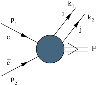
Figure 2: ${\cal O}(\alpha_{\mathrm{S}}^{2})$ contribution from double real emission.

and the corresponding matrix element is denoted by ${\cal M}^{(0)}_{c{\bar{c}}\rightarrow ij\,F}(p_{1},p_{2},k_{1},k_{2},\phi)$. The usual invariants are defined as

$$s=(p_{1}+p_{2})^{2}~{}~{}~{}~{}t=(p_{1}-q)^{2}~{}~{}~{}~{}u=(p_{2}-q)^{2}~{}~{}~{}~{}s_{2}=(k_{1}+k_{2})^{2}\,,$$ (49)

and fulfill the following relations

$$s+t+u=Q^{2}+s_{2}~{}~{}~{}~{}~{}~{}~{}~{}~{}~{}~{}~{}q_{T}^{2}=\frac{ut-s_{2}Q^{2}}{s}.$$ (50)

In terms of these invariants, the real contribution to the cross section at fixed $q_{T}^{2}$ is given by

$$\frac{d\sigma_{c{\bar{c}}\rightarrow ij\,F}}{dq_{T}^{2}dQ^{2}d\phi}=\int\frac{|{\cal M}^{(0)}_{c{\bar{c}}\rightarrow ij\,F}(p_{1},p_{2},k_{1},k_{2},\phi)|^{2}}{2s}\frac{(s_{2}q_{T}^{2})^{-\epsilon}}{(4\pi)^{4-2\epsilon}\Gamma(1-2\epsilon)}\frac{du}{Q^{2}-u}\frac{d\Omega}{2\pi}$$ (51)

where $d\Omega$ is

$$d\Omega=\sin\theta_{2}^{-2\epsilon}d\theta_{2}\sin\theta_{1}^{1-2\epsilon}d\theta_{1}\,,$$ (52)

with the angles defined in the frame where the partons corresponding to momentum $k_{1}$ and $k_{2}$ are back-to-back [15].

We see from Eq. (51) that the first step of the calculation involves the integration over the two angles. The integrals needed here are typical of heavy quark production at NLO and most of them can be found in Refs. [37, 38]. The results of the angular integrals contain poles up to $1/\epsilon$ while terms that develop an extra additional singularity as $s_{2}\rightarrow 0$ have to be computed up to ${\cal O}(\epsilon)$.

The second step is the integration over $u$ (or $s_{2}$). The integration limits are given by the two roots $u_{max}$ and $u_{min}$ in Equation (25). At this point, it is convenient to define the ‘symmetric’ value for which $u=t$

$$u_{0}=Q^{2}-\sqrt{s(q_{T}^{2}+Q^{2})}\,.$$ (53)

This value of $u$ corresponds also to the maximum of $s_{2}$

$$s_{2}^{max}\equiv A=Q^{2}\frac{1+z-2\sqrt{1+q_{T}^{2}/Q^{2}}\sqrt{z}}{z}$$ (54)

and, in the CM frame of $p_{1}$ and $p_{2}$, to the configuration where $q_{z}=0$. The singularity in $s_{2}$ is made manifest by use of the identity

$$s_{2}^{-1-\epsilon}=-\frac{1}{\epsilon}\delta(s_{2})\left(1-\epsilon\log A+\frac{1}{2}\epsilon^{2}\log^{2}A\right)+\frac{1}{(s_{2})_{A+}}-\epsilon\left(\frac{\log s_{2}}{s_{2}}\right)_{A+}+{\cal O}(\epsilon^{2})\,,$$ (55)

with the distributions defined as:

$$\int_{0}^{A}ds_{2}\frac{f(s_{2})}{(s_{2})_{A+}}=\int_{0}^{A}\frac{ds_{2}}{s_{2}}(f(s_{2})-f(0))$$ (56)

$$\int_{0}^{A}ds_{2}~{}f(s_{2})\left(\frac{\log s_{2}}{s_{2}}\right)_{A+}=\int_{0}^{A}~{}ds_{2}~{}\frac{\log s_{2}}{s_{2}}(f(s_{2})-f(0))\,.$$ (57)

In order to obtain $\Sigma(N)$ one finally has to integrate over $z$, keeping only the terms that do not vanish in the small-$q_{T}$ limit. At the beginning we consider only the $N=0$ moment. We will later show how to perform the calculation for general $N$, once one moment is known, in a simpler way. Notice that after implementing the regularization of the $s_{2}=0$ singularities using Eq. (55), the last two integrals can be performed directly in four-dimensions, since the small transverse momentum $q_{T}$ acts as a regulator of other possible singularities.

The double real contributions to (the non-singlet part of) $\Sigma^{(2)}_{q{\bar{q}}}(N)$ fall into three classes, according to the possible different final states:

• $q+{\bar{q}}\rightarrow{\bar{q}}+q+F$

• $q+q\rightarrow q+q+F$

• $q+{\bar{q}}\rightarrow g+g+F$   .

Notice that the $q+q\rightarrow q+q+F$ is needed to form the non-singlet combination.

As we did at ${\cal O}(\alpha_{\mathrm{S}})$, to study the small $q_{T}$ behaviour of $\Sigma$ we will rely on the structure of soft and collinear singularities of the corresponding QCD matrix element. In principle there are, of course, configurations where the two final state partons are hard and emitted back-to-back with small total transverse momentum. Nevertheless, these configurations do not produce any singularities when $q_{T}\rightarrow 0$ and thus may be neglected. Finally, notice that we consider only double singularities, i.e. configurations where two extra partons are either collinear or soft, without caring about single singularities. Configurations with only one collinear or soft parton (and the other hard) do not contribute to $\Sigma^{(2)}$ since the system $F$ is not emitted with small $q_{T}$ in such case.

4.1.1 Contribution from $q{\bar{q}}$ and $qq$ emission

For the $q+{\bar{q}}\rightarrow{\bar{q}}+q+F$ contribution we have three singular regions at ${\cal O}(\alpha_{\mathrm{S}}^{2})$ [19]:

• first triple-collinear region: $k_{1}p_{1}\sim k_{2}p_{1}\sim k_{1}k_{2}\rightarrow 0$;

• second triple-collinear region: $k_{1}p_{2}\sim k_{2}p_{2}\sim k_{1}k_{2}\rightarrow 0$;

• double-soft region: $k_{1},k_{2}\rightarrow 0$   .

In the first region the singularity is controlled by the following collinear factorization formula [18, 24, 19]

$$|{\cal M}^{(0)}_{q{\bar{q}}\rightarrow q{\bar{q}}F}(p_{1},p_{2},k_{1},k_{2},\phi)|^{2}\simeq\frac{(8\pi\mu^{2\epsilon}\alpha_{\mathrm{S}})^{2}}{u^{2}}{\hat{P}}_{q\rightarrow{\bar{q}}_{1}q_{2}(q_{3})}|{\cal M}_{q{\bar{q}}\rightarrow F}^{(0)}(z_{3}p_{1},p_{2},\phi)|^{2}\,,$$ (58)

where ${\hat{P}}_{q\rightarrow{\bar{q}}_{1}q_{2}(q_{3})}$ is the splitting function that controls the collinear decay of an initial state quark of momentum $p_{1}$ into a final state quark-antiquark pair ${\bar{q}}_{1}q_{2}$ of momenta $k_{1}$ and $k_{2}$ and the ‘off-shell’ quark $q_{3}$ that participates in the hard cross section.. The explicit expression of ${\hat{P}}_{q\rightarrow{\bar{q}}_{1}q_{2}(q_{3})}$ is obtained from the one of ${\hat{P}}_{{\bar{q}}_{1}q_{2}q_{3}}$, the splitting function for the decay of a (‘off-shell’) quark into a final state quark-antiquark pair plus a quark, given in Eq. (A.1), with the following definitions

$$s_{12}=s_{2}~{}~{}~{}s_{13}=-2p_{1}k_{1}~{}~{}~{}s_{23}=-2p_{1}k_{2}$$

$$x_{1}=-z_{1}/z_{3}~{}~{}~{}x_{2}=-z_{2}/z_{3}~{}~{}~{}x_{3}=1/z_{3}\,,$$ (59)

where $z_{1}$ and $z_{2}$ are the momentum fractions of ${\bar{q}}_{1}$ and $q_{2}$ ($z_{3}=1-z_{1}-z_{2}$). Notice that Eq. (4.1.1) corresponds to the following transformation:

$$r_{1}\rightarrow k_{1},~{}~{}~{}~{}r_{2}\rightarrow k_{2},~{}~{}~{}~{}r_{3}\rightarrow-p_{1}\,,$$ (60)

applied to the expression in Eq. (A.1) to cross the ‘off-shell’ parton to the final state.

A formula similar to Eq. (58) can be written in the second collinear region.

In the double-soft region the factorization formula is instead [19]:

$$|{\cal M}^{(0)}_{q{\bar{q}}\rightarrow q{\bar{q}}F}\,(p_{1},p_{2},k_{1},k_{2},\phi)|^{2}\simeq(4\pi\mu^{2\epsilon}\alpha_{\mathrm{S}})^{2}\,C_{F}\,T_{R}\;\Big{(}{\cal I}_{11}+{\cal I}_{22}-2\,{\cal I}_{12}\Big{)}\;|{\cal M}^{(0)}_{q{\bar{q}}\rightarrow F}\,(\phi)|^{2}\,,$$ (61)

where

$${\cal I}_{ij}={\cal I}_{ij}(k_{1},k_{2})=\frac{p_{i}k_{1}\;p_{j}k_{2}+p_{j}k_{1}\;p_{i}k_{2}-p_{i}p_{j}\;k_{1}k_{2}}{(k_{1}k_{2})^{2}\,p_{i}(k_{1}+k_{2})\;p_{j}(k_{1}+k_{2})}\,.$$ (62)

The reader can easily check that by defining the momentum fractions in Eq. (4.1.1) as

$$z_{1}=\frac{k_{1}p_{2}}{p_{1}p_{2}}~{}~{}~{}~{}~{}z_{2}=\frac{k_{2}p_{2}}{p_{1}p_{2}}$$ (63)

Eq. (58) correctly keeps into account also the double-soft limit in Eq. (61). Thus, at least outside the second collinear region, the factorization formula (58) with the definitions (63) correctly gives the full singular behaviour in this channel.

The strategy to perform the calculation is the following. We use Eq. (58) to approximate the matrix element in its region of validity and compute its contribution to $\Sigma^{(2)R}_{q{\bar{q}}}(0)$ by integrating only in half of the phase space, that is from $u_{0}$ to $u_{max}$. The remaining region, which is obtained by exchanging $u\leftrightarrow t$, will give , due to the symmetry of the initial state, exactly the same contribution and it is taken into account by multiplying the computed result by 2. As it happens at leading order, the information on the process, embodied in the Born matrix element is completely factored out in the calculation and disappears in $\Sigma$. In fact the Born matrix element can be fully written in terms of the (fixed) kinematics of the final state particles $|{\cal M}^{(0)}_{q{\bar{q}}\rightarrow F}(z_{3}p_{1},p_{2},\phi)|^{2}\equiv|{\cal M}_{q{\bar{q}}\rightarrow F}^{(0)}(\phi)|^{2}$.

For the $q+q\rightarrow q+q+F$ contribution, needed to form the non-singlet contribution in Eq. (21), there are only two singular configurations:

• first triple-collinear region: $k_{1}p_{1}\sim k_{2}p_{1}\sim k_{1}k_{2}\rightarrow 0$;

• second triple-collinear region: $k_{1}p_{2}\sim k_{2}p_{2}\sim k_{1}k_{2}\rightarrow 0$   .

For the first collinear region we can write:

$$|{\cal M}^{(0)}_{qq\rightarrow qqF}(p_{1},p_{2},k_{1},k_{2},\phi)|^{2}\simeq\frac{(8\pi\mu^{2\epsilon}\alpha_{\mathrm{S}})^{2}}{u^{2}}{\hat{P}}_{q\rightarrow q_{1}q_{2}({\bar{q}}_{3})}|{\cal M}^{(0)}_{q{\bar{q}}\rightarrow F}(p_{1},z_{3}p_{2},\phi)|^{2}\,.$$ (64)

Here ${\hat{P}}_{q\rightarrow q_{1}q_{2}({\bar{q}}_{3})}$ is now the splitting function which controls the collinear decay of an initial state quark into a final state $qq$ pair. The explicit expression for ${\hat{P}}_{q\rightarrow q_{1}q_{2}({\bar{q}}_{3})}$ can be obtained from the expression of ${\hat{P}}_{{\bar{q}}_{1}q_{2}q_{3}}$ in Eq. (A.1) with the following definitions

$$s_{12}=-2p_{1}k_{2}~{}~{}~{}s_{13}=-2p_{1}k_{1}~{}~{}~{}s_{23}=s_{2}$$

$$x_{1}=1/z_{3}~{}~{}~{}x_{2}=-z_{2}/z_{3}~{}~{}~{}x_{3}=-z_{1}/z_{3}\,,$$ (65)

i.e., corresponding to the crossing transformation:

$$r_{1}\rightarrow-p_{1},~{}~{}~{}~{}r_{2}\rightarrow k_{2},~{}~{}~{}~{}r_{3}\rightarrow k_{1}\,,$$ (66)

and similarly for the second collinear configuration (with $p_{1}\leftrightarrow p_{2}$). There is a partial cancellation between the $C_{F}T_{R}$ contribution to $\Sigma_{q{\bar{q}}}^{(2)}$ from Eqs. (58) and (64), due to the non-singlet combination. Once this cancellation is carried out, the part corresponding to the production of ‘non-identical’ partons in the $q{\bar{q}}$ channel gives the following $C_{F}T_{R}$ contribution to $\Sigma_{q{\bar{q}}}^{(2)}$ :

$$\Sigma^{(2)R}_{q{\bar{q}}\,{\rm(nid)}}(0)=C_{F}n_{f}T_{R}\,{\cal K}\Bigg{[}-\frac{2}{3}\frac{1}{\epsilon}{\cal F}_{q{\bar{q}}}(0,\epsilon)-\frac{4}{3}\log^{2}\frac{Q^{2}}{q_{T}^{2}}-\frac{2}{9}\log\frac{Q^{2}}{q_{T}^{2}}+1+\frac{2}{9}\pi^{2}\Bigg{]}\,,$$ (67)

where

$${\cal K}=\frac{1}{\Gamma(1-2\epsilon)}\left(\frac{4\pi\mu^{2}}{q_{T}^{2}}\right)^{\epsilon}\left(\frac{4\pi\mu^{2}}{Q^{2}}\right)^{\epsilon}\,,$$ (68)

and the explicit expression of function ${\cal F}_{q{\bar{q}}}(0,\epsilon)$, defined in Eq. (3) is

$${\cal F}_{q{\bar{q}}}(0,\epsilon)=2\log\frac{Q^{2}}{q_{T}^{2}}-3-\epsilon\,.$$ (69)

At the beginning of Eq. (67) we have isolated a divergent term which will be cancelled by a similar one appearing in the virtual contribution.

The part corresponding to the production of ‘identical’ partons in the $q{\bar{q}}$ channel gives also a $C_{F}(C_{F}-C_{A}/2)$ contribution, which does not contain any $\log Q^{2}/q_{T}^{2}$ term. Therefore, there is a great simplification in the calculation since $q_{T}$ can be set to zero just after performing the angular integrations. We find:

$$\Sigma^{(2)R}_{q{\bar{q}}\,{\rm(id)}}(0)=C_{F}(C_{F}-\frac{1}{2}C_{A})\Big{(}-6+2\pi^{2}-16\zeta(3)\Big{)}\,.$$ (70)

The calculation of the $qq$ contribution can be performed with exactly the same strategy as for the $q{\bar{q}}$ channel. After the $C_{F}T_{R}$ contribution has been cancelled with a similar one in the $q{\bar{q}}$ channel only a contribution proportional to $C_{F}(C_{F}-C_{A}/2)$ remains

$$\Sigma^{(2)R}_{q{\bar{q}}({\rm qq})}(0)=-C_{F}(C_{F}-\frac{1}{2}C_{A})\left(\frac{13}{2}-\pi^{2}+4\zeta(3)\right)\,.$$ (71)

4.1.2 Contribution from $gg$ emission

The calculation of the double-gluon emission correction to $\Sigma_{R}^{(2)}$ is more difficult, because it is not possible to keep into account all possible singular configurations by using only the triple-collinear splitting functions. We will divide the calculation in two parts, according to the corresponding colour factors. First we will consider the non-abelian, $C_{F}C_{A}$ term, which turns out to be simpler, and finally the abelian, $C_{F}^{2}$ part.

$C_{F}C_{A}$ contribution

For this colour structure there are three singular regions to be considered [19]

• first triple-collinear region: $k_{1}p_{1}\sim k_{2}p_{1}\sim k_{1}k_{2}\rightarrow 0$;

• second triple-collinear region: $k_{1}p_{2}\sim k_{2}p_{2}\sim k_{1}k_{2}\rightarrow 0$;

• double-soft region: $k_{1},k_{2}\rightarrow 0$   .

We point out that, as discussed in Ref. [19], thanks to the coherence properties of soft-gluon radiation, the soft-collinear region does not give any contribution proportional to $C_{F}C_{A}$ (see later).

In the first collinear region the singularity is controlled by the following factorization formula:

$$|{\cal M}^{(0)}_{q{\bar{q}}\rightarrow gg\,F}(p_{1},p_{2},k_{1},k_{2},\phi)|_{{\rm nab}}^{2}\simeq\frac{(8\pi\mu^{2\epsilon}\alpha_{\mathrm{S}})^{2}}{u^{2}}C_{F}C_{A}{\hat{P}}^{{\rm(nab)}}_{q\rightarrow g_{1}g_{2}(q_{3})}|{\cal M}^{(0)}_{q{\bar{q}}\rightarrow F}(z_{3}p_{1},p_{2},\phi)|^{2}\,,$$ (72)

where ${\hat{P}}^{{\rm(nab)}}_{q\rightarrow g_{1}g_{2}(q_{3})}$ is the non-abelian part of the splitting function that controls the collinear decay of an initial state quark into a final state gluon pair. This function can be obtained from Eq. (Appendix: Triple-collinear splitting functions) with the replacement in Eq. (4.1.1).

A similar formula to Eq. (72) can be written in the second collinear region (by $p_{1}\leftrightarrow p_{2}$ exchange).

In the double-soft region the factorization formula is instead (see Eq. (A.3) of Ref. [19]):

$$|{\cal M}^{(0)}_{q{\bar{q}}\rightarrow ggF}(p_{1},p_{2},k_{1},k_{2},\phi)|_{{\rm nab}}^{2} \simeq(4\pi\mu^{2\epsilon}\alpha_{\mathrm{S}})^{2}\,C_{F}\,C_{A}$$

$$\cdot\left(2\,{\cal S}_{12}(k_{1},k_{2})-{\cal S}_{11}(k_{1},k_{2})-{\cal S}_{22}(k_{1},k_{2})\right)|{\cal M}_{q{\bar{q}}\rightarrow F}\,(\phi)|^{2}\,,$$ (73)

where the non-abelian double-soft function reads

$${\cal S}_{ij}(k_{1},k_{2}) =\frac{(1-\epsilon)}{(k_{1}k_{2})^{2}}\;\frac{p_{i}k_{1}\;p_{j}k_{2}+p_{i}k_{2}\;p_{j}k_{1}}{p_{i}(k_{1}+k_{2})\;p_{j}(k_{1}+k_{2})}$$

$$-\frac{(p_{i}p_{j})^{2}}{2p_{i}k_{1}\;p_{j}k_{2}\;p_{i}k_{2}\;p_{j}k_{1}}\left[2-\frac{p_{i}k_{1}\;p_{j}k_{2}+p_{i}k_{2}\;p_{j}k_{1}}{p_{i}(k_{1}+k_{2})\;p_{j}(k_{1}+k_{2})}\right]$$ (74)

$$+\frac{p_{i}p_{j}}{2k_{1}k_{2}}\left[\frac{2}{p_{i}k_{1}\;p_{j}k_{2}}+\frac{2}{p_{j}k_{1}\;p_{i}k_{2}}\right.$$

$$-\left.\frac{1}{p_{i}(k_{1}+k_{2})\;p_{j}(k_{1}+k_{2})}\left(4+\frac{(p_{i}k_{1}\;p_{j}k_{2}+p_{i}k_{2}\;p_{j}k_{1})^{2}}{p_{i}k_{1}\;p_{j}k_{2}\;p_{i}k_{2}\;p_{j}k_{1}}\right)\right]\;\;.$$

As it happens in the $q{\bar{q}}$ and $qq$ channels, it turns out that by defining the momentum fractions of the gluons as in Eq. (63), the factorization formula in Eq. (72) correctly accounts also for the double-soft configuration. Furthermore, we have verified that Eq. (72) does not introduce any additional spurious singularities in the other infrared configurations. Thus for this colour structure the situation is similar to the one in the $q{\bar{q}}$ and $qq$ channels and we can follow the same strategy. We approximate the non-abelian part of the matrix element in the region from $u_{0}$ to $u_{max}$ using Eq. (72). We first perform the angular integrals and then, exploiting the $p_{1}\leftrightarrow p_{2}$ symmetry, do the remaining $u$ and $z$ integrations only over half of the phase space, i.e. with $u$ from $u_{0}$ to $u_{max}$.

In order to perform the last two steps, that are considerably more complicated than in the case of $q{\bar{q}}$ emission, we developed Mathematica [39] programs that are able to handle the cumbersome intermediate expressions in the small $q_{T}$ limit.

The result is

$$\Sigma^{(2)R}_{q{\bar{q}}({\rm ggnab})}(0) =C_{F}C_{A}\,{\cal K}\Bigg{[}\left(\frac{1}{\epsilon^{2}}+\frac{1}{\epsilon}\left(\frac{11}{6}+\log\frac{Q^{2}}{q_{T}^{2}}\right)\right){\cal F}_{q{\bar{q}}}(0,\epsilon)$$

$$+\log^{3}\frac{Q^{2}}{q_{T}^{2}}+\frac{13}{6}\log^{2}\frac{Q^{2}}{q_{T}^{2}}+\left(\frac{35}{18}-\frac{2}{3}\pi^{2}\right)\log\frac{Q^{2}}{q_{T}^{2}}+4\zeta(3)-2+\frac{7}{18}\pi^{2}\Bigg{]}\,,$$ (75)

in agreement with Ref. [40]. The first line of Eq. (4.1.2) comes from the singular $\delta(s_{2})$ terms and will be exactly cancelled by a contribution appearing in the virtual correction.

$C_{F}^{2}$ contribution

For this colour structure there are six singular regions (plus the ones generated from permutations like $k_{1}\leftrightarrow k_{2}$) to be considered [18, 19]

• first triple-collinear region: $k_{1}p_{1}\sim k_{2}p_{1}\sim k_{1}k_{2}\rightarrow 0$;

• second triple-collinear region: $k_{1}p_{2}\sim k_{2}p_{2}\sim k_{1}k_{2}\rightarrow 0$;

• double-soft region: $k_{1},k_{2}\rightarrow 0$;

• first soft-collinear region: $k_{1}\rightarrow 0$, $k_{2}p_{1}\rightarrow 0$;

• second soft-collinear region: $k_{1}\rightarrow 0$, $k_{2}p_{2}\rightarrow 0$;

• double-collinear region: $k_{1}p_{1}\rightarrow 0$, $k_{2}p_{2}\rightarrow 0$.

In the first region the singularity is controlled by the collinear factorization formula:

$$|{\cal M}_{q{\bar{q}}\rightarrow gg\,F}(p_{1},p_{2},k_{1},k_{2},\phi)|_{{\rm ab}}^{2}\simeq\frac{(8\pi\mu^{2\epsilon}\alpha_{\mathrm{S}})^{2}}{u^{2}}C_{F}^{2}{\hat{P}}^{{\rm(ab)}}_{q\rightarrow g_{1}g_{2}(q_{3})}|{\cal M}^{(0)}_{q{\bar{q}}\rightarrow F}(z_{3}p_{1},p_{2},\phi)|^{2}\,,$$ (76)

where ${\hat{P}}^{{\rm(ab)}}_{q\rightarrow g_{1}g_{2}(q_{3})}$ is the abelian part of the splitting function that controls the collinear decay of an initial state quark into a final state gluon pair. This function can be obtained from Eq. (Appendix: Triple-collinear splitting functions) with the replacement in Eq. (4.1.1).

In the double-soft region the factorization formula is obtained by factorizing the two eikonal factors for independent gluon emissions (see Eq. (A.3) of Ref. [19]):

$$|{\cal M}^{(0)}_{q{\bar{q}}\rightarrow ggF}(p_{1},p_{2},k_{1},k_{2},\phi)|_{{\rm ab}}^{2}\simeq(4\pi\mu^{2\epsilon}\alpha_{\mathrm{S}})^{2}\,16C_{F}^{2}\,{\cal S}_{12}(k_{1}){\cal S}_{12}(k_{2})|{\cal M}^{(0)}_{q{\bar{q}}\rightarrow F}(\phi)|^{2}\,,$$ (77)

with ${\cal S}_{12}(k)$ defined in Eq. (32).

In the soft-collinear region, say when $k_{2}\rightarrow 0$ and $k_{1}p_{1}\rightarrow 0$ we have instead (see Eq. (A.5) of [19]):

$$|{\cal M}^{(0)}_{q{\bar{q}}\rightarrow ggF}(p_{1},p_{2},k_{1},k_{2},\phi)|^{2} \simeq(4\pi\mu^{2\epsilon}\alpha_{\mathrm{S}})^{2}\frac{2C_{F}}{(1-z_{1})\,p_{1}k_{1}}\frac{(p_{1}-k_{1})p_{2}}{(p_{1}-k_{1})k_{2}\,p_{2}k_{2}}\,{\hat{P}}_{qq}(1-z_{1},\epsilon)$$

$$\cdot|{\cal M}^{(0)}_{q{\bar{q}}\rightarrow F}\left((1-z_{1})p_{1},p_{2},\phi\right)|^{2}\,,$$ (78)

where $z_{1}$ is the momentum fraction of the collinear gluon of momentum $k_{1}$ and can be identified with the one parametrizing the triple collinear splitting in Eq. (76). Notice that, since the soft gluon of momentum $k_{2}$ does not resolve the pair of collinear partons, there is no non-abelian contribution in Eq. (4.1.2).

In the double-collinear region we have, when e.g. $k_{1}p_{1}\rightarrow 0$ and $k_{2}p_{2}\rightarrow 0$:

$$|{\cal M}^{(0)}_{q{\bar{q}}\rightarrow ggF}(p_{1},p_{2},k_{1},k_{2},\phi)|^{2} \simeq\frac{(4\pi\mu^{2\epsilon}\alpha_{\mathrm{S}})^{2}}{(1-z_{1})p_{1}k_{1}\,(1-{\bar{z}}_{2})p_{2}k_{2}}\,{\hat{P}}_{qq}\left(1-z_{1},\epsilon\right){\hat{P}}_{qq}\left(1-{\bar{z}}_{2},\epsilon\right)$$

$$\cdot|{\cal M}^{(0)}_{q{\bar{q}}\rightarrow F}\left((1-z_{1})p_{1},(1-{\bar{z}}_{2})p_{2},\phi\right)|^{2}\,,$$ (79)

where $z_{1}$ and ${\bar{z}}_{2}$ here represent the momentum fractions (see below) involved in the two collinear splittings.

As it happens for the $C_{F}C_{A}$ contribution, Eq. (76) supplemented with the definitions (63) is able to approximate correctly also the double-soft and soft-collinear regions in half of the phase space. But, at variance with the $C_{F}C_{A}$ case, the same formula cannot describe correctly the double-collinear region, since that one corresponds to the emission of gluons from different legs, i.e., with a kinematical configuration completely different from the triple-collinear case. Therefore, the strategy followed for the other colour factors does not work in this case.

In order to overcome this problem there are in principle two strategies. The first one is to split the phase space in order to isolate the double-collinear region and perform the calculation separately for its contribution using the expression in Eq. (4.1.2). The second is to modify Eq. (76) in order to enforce the correct singular behaviour in all possible limits. We decided to follow the second strategy and for that we have first studied Eq. (76) with the definitions (63) and isolated the terms that do, incorrectly, contribute (terms with $x_{2}$ in the denominator) when the collinear gluons are emitted from the different legs. In this way, we were able to find a slight modification of ${\hat{P}}^{{\rm(ab)}}_{g_{1}g_{2}q_{3}}$ in Eq. (Appendix: Triple-collinear splitting functions) that allows to take into account the double-collinear region without spoiling the behaviour in the other regions as

$${\hat{D}}_{g_{1}g_{2}q_{3}}^{{\rm(ab)}} =\Biggl{\{}\frac{s_{123}^{2}}{2s_{13}s_{23}}x_{3}\left[\left(\frac{1+x_{3}^{2}}{x_{1}x_{2}}-\epsilon\frac{x_{1}^{2}+x_{2}^{2}}{x_{1}x_{2}}\right)f_{q}({\bar{z}}_{1})f_{q}({\bar{z}}_{2})-\epsilon(1+\epsilon)\right]$$

$$+\frac{s_{123}}{s_{13}}\Biggl{[}\left(\frac{x_{3}(1-x_{1})+(1-x_{2})^{3}}{x_{1}x_{2}}-\epsilon(x_{1}^{2}+x_{1}x_{2}+x_{2}^{2})\frac{1-x_{2}}{x_{1}x_{2}}\right)f_{q}({\bar{z}}_{2})+\epsilon^{2}(1+x_{3})\Biggr{]}$$

$$+(1-\epsilon)\left[\epsilon-(1-\epsilon)\frac{s_{23}}{s_{13}}\right]\Biggr{\}}+(1\leftrightarrow 2)\;\;.$$ (80)

With respect to the expression of ${\hat{P}}_{g_{1}g_{2}q_{3}}^{\rm(ab)}$ of Eq. (Appendix: Triple-collinear splitting functions), the only difference is due to the introduction of the extra factors $f_{q}(z)$. The function $f_{a}(z)$, anticipating that a similar approach will be followed in the gluonic channel, is defined by

$$f_{a}(z)=\frac{z}{2C_{a}(1-z)}{\hat{P}}_{aa}(1-z,\epsilon)~{}~{}~{}~{}~{}a=q,g\,,$$ (81)

where ${\hat{P}}_{aa}$ are the collinear splitting kernels in Eqs. (28,29).

The function ${\hat{D}}_{g_{1}g_{2}q_{3}}^{{\rm(ab)}}$ depends on the new momentum fractions ${\bar{z}}_{1}$ and ${\bar{z}}_{2}$ of the gluons with respect to the incoming antiquark of momentum $p_{2}$. These momentum fractions should be the ones relevant for the double-collinear limit. Our improved factorization formula is, outside the second triple-collinear region given by

$$|{\cal M}^{(0)}_{q{\bar{q}}\rightarrow gg\,F}(p_{1},p_{2},k_{1},k_{2},\phi)|_{{\rm ab}}^{2}\simeq\frac{(8\pi\mu^{2\epsilon}\alpha_{\mathrm{S}})^{2}}{u^{2}}C_{F}^{2}{\hat{D}}^{{\rm(ab)}}_{q\rightarrow g_{1}g_{2}(q_{3})}|{\cal M}^{(0)}_{q{\bar{q}}\rightarrow F}(z_{3}p_{1},p_{2},\phi)|^{2}\,,$$ (82)

where ${\hat{D}}^{{\rm(ab)}}_{q\rightarrow g_{1}g_{2}(q_{3})}$ is obtained from ${\hat{D}}_{g_{1}g_{2}q_{3}}^{{\rm(ab)}}$ in Eq. (4.1.2) with the definitions in Eqs. (4.1.1),(63) and by setting

$${\bar{z}}_{1}=\frac{p_{1}k_{1}}{p_{1}p_{2}}~{}~{}~{}~{}~{}~{}~{}~{}{\bar{z}}_{2}=\frac{p_{1}k_{2}}{p_{1}p_{2}}\,.$$ (83)

With Eq. (82) we can consistently approximate the relevant matrix element in the region from $u_{0}$ to $u_{max}$ as we did in the other channels, keeping into account all the singular regions. In fact in the triple-collinear region ${\bar{z}}_{1},{\bar{z}}_{2}\rightarrow 0$ and $f_{q}({\bar{z}}_{1}),f_{q}({\bar{z}}_{2})\rightarrow 1$. Therefore, in this limit Eq. (82) reduces to Eq. (76). The factors $f_{q}(z)$ become relevant in the double-collinear region, since they ensure that the correct limit is recovered when $p_{1}k_{1}\rightarrow 0$ and $p_{2}k_{2}\rightarrow 0$ (and the same for $k_{1}\leftrightarrow k_{2}$).

Notice that the modification of the triple-collinear formula does not spoil the process independence of our calculation: it just allows to write an ‘improved’ formula that correctly interpolates all possible (double-) collinear and soft singularities in the region of phase space where we have to integrate it. Therefore, with this approach we can avoid to split the phase space in regions where different approximations should be applied.

It is worth noticing that the modification in Eq. (4.1.2) makes the calculation more involved already at the level of the angular integrals, mostly due to the introduction of the ‘new’ momentum fractions ${\bar{z}}_{1}$ and ${\bar{z}}_{2}$.

For this colour structure we have to subtract the contribution from the factorization counterterm, which can be written as

$$\frac{d\sigma_{FCT}}{dq_{T}^{2}dQ^{2}d\phi} = \frac{\alpha_{\mathrm{S}}}{2\pi}\int\frac{dx}{x}R(x,\mu_{F}^{2})\left(\frac{d\sigma(p_{1},p_{2},\phi,k)}{dq_{T}^{2}dQ^{2}d\phi}\right)_{p_{1}\rightarrow xp_{1}}$$ (84)

$$+ \frac{\alpha_{\mathrm{S}}}{2\pi}\int\frac{dx}{x}R(x,\mu_{F}^{2})\left(\frac{d\sigma(p_{1},p_{2},\phi,k)}{dq_{T}^{2}dQ^{2}d\phi}\right)_{p_{2}\rightarrow xp_{2}}\,,$$

where ${d\sigma(p_{1},p_{2},\phi,k)}$ corresponds to the cross section for the production of $F$ and only one extra gluon (see Eq. (24)) and

$$R(x,\mu_{F}^{2})=-\frac{1}{\epsilon}P_{qq}^{AP}(x)\frac{\Gamma(1-\epsilon)}{\Gamma(1-2\epsilon)}\left(\frac{4\pi\mu^{2}}{\mu_{F}^{2}}\right)^{\epsilon}\,,$$ (85)

with $P_{qq}^{AP}(z)=\left(\hat{P}_{qq}(z,0)\right)_{+}=C_{F}\left(\frac{1+z^{2}}{1-z}\right)_{+}$ the regularized AP splitting function and $\mu_{F}$ the factorization scale. In the limit of small $q_{T}$ and after taking moments with respect to $z$, the contribution from the counterterm factorizes as

$$\Sigma^{(2)}_{q{\bar{q}}(FCT)}(N)=2\,C_{F}{\cal F}_{q{\bar{q}}}(N,\epsilon)\left[-\frac{1}{\epsilon}{\cal K}\left(\frac{Q^{2}}{\mu_{F}^{2}}\right)^{\epsilon}\gamma_{qq}^{(1)}(N)\right]\,.$$ (86)

where ${\cal F}_{q{\bar{q}}}(N,\epsilon)$ and ${\cal K}$ are defined in Eqs. (3) and (68), respectively. Therefore, in the $q_{T}\rightarrow 0$ limit also the contribution of the factorization counterterm becomes process independent.

Our final result for the $N=0$ moment of the factorized contribution $\tilde{\Sigma}^{(2)R}_{q{\bar{q}}({\rm ggab})}(0)\equiv\Sigma^{(2)R}_{q{\bar{q}}({\rm ggab})}(0)-\Sigma^{(2)}_{q{\bar{q}}(FCT)}(0)$ is:

$$\tilde{\Sigma}^{(2)R}_{q{\bar{q}}({\rm ggab})}(0) =C_{F}\,{\cal K}\Bigg{[}\left(\frac{2}{\epsilon^{2}}+\frac{3}{\epsilon}\right)C_{F}\,{\cal F}_{q{\bar{q}}}(0,\epsilon)+\frac{2}{\epsilon}\int_{0}^{1}2{\hat{P}}_{qq}(z,\epsilon)\log z\Bigg{]}$$

$$+C_{F}^{2}\,\Bigg{[}-2\log^{3}\frac{Q^{2}}{q_{T}^{2}}+9\log^{2}\frac{Q^{2}}{q_{T}^{2}}-\left(2+\frac{2}{3}\pi^{2}\right)\log\frac{Q^{2}}{q_{T}^{2}}+16\zeta(3)-\pi^{2}-\frac{43}{4}\Bigg{]}\,,$$ (87)

in agreement with the result of Ref. [40] for Drell–Yan. Notice that since $\gamma_{qq}^{(1)}(0)=0$ there is no contribution from the factorization counterterm to $\hat{\Sigma}^{(2)R}_{q{\bar{q}}(\rm{ggab})}(0)$. As we did for the other colour factors, we have isolated in the first line of Eq. (4.1.2) the part that will be cancelled by a similar term in the virtual contribution.

A comment to the results obtained so far is in order. The formulae in Eqs. (67), (70), (71), (4.1.2), (4.1.2) show that the contribution to $\Sigma_{q{\bar{q}}}(0)$ from double real emission are actually independent on the specific process in (1). This feature of the double real emission, which is due to the universality of soft and collinear radiation, will persist also in the gluon channel. The explicit results obtained so far all agree with the ones obtained for Drell–Yan in Ref. [40].

4.2 Virtual corrections

The second part on the calculation of $\Sigma_{q{\bar{q}}}(N)$ involves the (one-loop) virtual corrections to single-gluon emission. The corresponding soft and collinear limits have been recently studied in Refs. [21, 22, 23]. The kinematics is the same as at ${\cal O}(\alpha_{\mathrm{S}})$ and the singularities originated by the same configurations discussed above Eq. (27). In the first collinear region the interference between the tree-level and one-loop contributions to single gluon emission behaves as [21, 22]

$${\cal M}^{(0)\dagger}_{q{\bar{q}}\rightarrow g\,F} \left(p_{1},p_{2},k,\phi\right){\cal M}_{q{\bar{q}}\rightarrow g\,F}^{(1)u}\left(p_{1},p_{2},k,\phi\right)+{\rm c.c.}\simeq\frac{4\pi\alpha_{\mathrm{S}}\mu^{2\epsilon}}{z_{1}p_{1}k}$$

$$\times\Big{[} {\hat{P}}_{qq}(z_{1},\epsilon)\left({\cal M}^{(0)\dagger}_{q{\bar{q}}\rightarrow F}\left(z_{1}p_{1},p_{2},\phi\right){\cal M}_{q{\bar{q}}\rightarrow F}^{(1)}\left(z_{1}p_{1},p_{2},\phi\right)+{\rm c.c.}\right)$$

$$+2g_{S}^{2}\left(\frac{4\pi\mu^{2}}{2p_{1}k}\right)^{\epsilon}{\hat{P}}^{(1)}_{q\rightarrow(q)g}(z_{1},\epsilon)|{\cal M}^{(0)}_{q{\bar{q}}\rightarrow F}\left(z_{1}p_{1},p_{2},\phi\right)|^{2}\Big{]}\,.$$ (88)

In Eq. (4.2) there are two terms. In the first one the tree-level splitting kernel ${\hat{P}}_{qq}(z_{1},\epsilon)$ is factorized with respect to the interference of the renormalized one-loop amplitude ${\cal M}_{q{\bar{q}}\rightarrow F}^{(1)}$ and the tree level one ${\cal M}^{(0)}_{q{\bar{q}}\rightarrow F}$.

The second term contains instead the unrenormalized one-loop correction to the splitting kernel ${\hat{P}}^{(1)}_{q\rightarrow(q)g}(z_{1},\epsilon)$ times the Born matrix element squared. The function ${\hat{P}}^{(1)}_{q\rightarrow(q)g}(z_{1},\epsilon)$ controls the one-loop collinear splitting of an initial state quark into a final state quark with momentum fraction $z_{1}$, in the CDR scheme. Its explicit expression can be derived from the results of Ref. [21, 22] and is up to ${\cal O}(\epsilon^{0})$:

$${\hat{P}}^{(1)}_{q\rightarrow(q)g}(x,\epsilon)=(1-x)^{-\epsilon}\frac{C_{\Gamma}}{(4\pi)^{2}}\Bigg{[} C_{A}{\hat{P}}_{qq}(x,\epsilon)\left(-\frac{1}{\epsilon^{2}}+\frac{1}{2}\log^{2}(1-x)+\mathop{\hbox{\rm Li}}\nolimits_{2}\frac{1}{1-x}-\mathop{\hbox{\rm Li}}\nolimits_{2}\,(1-x)\right)$$

$$+ C_{F}{\hat{P}}_{qq}(x,\epsilon)\left(-\frac{2}{\epsilon}\log(x)-2\log(x)\log(1-x)+2\mathop{\hbox{\rm Li}}\nolimits_{2}\,(1-x)\right)$$

$$+ C_{F}(C_{F}-C_{A})\,x\,\Bigg{]}\,,$$ (89)

where

$$C_{\Gamma}=\frac{\Gamma(1+\epsilon)\Gamma^{2}(1-\epsilon)}{\Gamma(1-2\epsilon)}\,.$$ (90)

A factorization formula similar to Eq. (4.2) holds when the gluon is radiated by the initial state antiquark.

Let us now consider the soft region. At one-loop order, for a general amplitude with $n$ hard partons, soft factorization formulae involve colour correlations between two and three hard momentum partons in the matrix element squared [23]. Nevertheless, in the case of only two hard partons the soft singularity is controlled by a simpler factorization formula (see Eq. (57) of Ref. [23])

$${\cal M}^{(0)\dagger}_{q{\bar{q}}\rightarrow g\,F}\left(p_{1},p_{2},k,\phi\right) {\cal M}_{q{\bar{q}}\rightarrow g\,F}^{(1)u}(p_{1},p_{2},k,\phi)+{\rm c.c.}\simeq 16\pi\alpha_{\mathrm{S}}\mu^{2\epsilon}\;C_{F}$$

$$\cdot\Bigg{(}{\cal S}_{12}(k)\left({\cal M}^{(0)\dagger}_{q{\bar{q}}\rightarrow F}(\phi){\cal M}^{(1)}_{q{\bar{q}}\rightarrow F}(\phi)+{\rm c.c.}\right)+{\cal S}^{(1)}_{12}(k)|{\cal M}^{(0)}_{q{\bar{q}}\rightarrow F}(\phi)|^{2}\Bigg{)}\,,$$ (91)

where

$${\cal S}_{12}^{(1)}(k)=-\frac{\alpha_{\mathrm{S}}}{2\pi}\,C_{A}\,{\cal S}_{12}(k)\frac{1}{\epsilon^{2}}\,\frac{\Gamma^{4}(1-\epsilon)\Gamma^{3}(1+\epsilon)}{\Gamma^{2}(1-2\epsilon)\Gamma(1+2\epsilon)}\left[4\pi\mu^{2}{\cal S}_{12}(k)\right]^{\epsilon}$$ (92)

is the unrenormalized one-loop correction to the tree-level eikonal factor. Likewise at ${\cal O}(\alpha_{\mathrm{S}})$ (see Eq. (31)), in Eq. (4.2) colour correlations are absent, and the factorization formula is similar in structure to the collinear one in Eq. (4.2).

One can verify that, as it happens at leading order, the factorization formula Eq. (4.2) with $z_{1}=z=Q^{2}/s$ correctly reproduces also the behaviour in the soft-region, given by Eq. (4.2).

Furthermore, by expressing $kp_{1}$ in terms of $q_{T}$ and using Lorentz invariance as we did at leading order, a single factorization formula in the small $q_{T}$ limit is obtained:

$${\cal M}^{(0)\dagger}_{q{\bar{q}}\rightarrow g\,F}\left(p_{1},p_{2},k,\phi\right){\cal M}^{(1)u}_{q{\bar{q}}\rightarrow g\,F} \left(p_{1},p_{2},k,\phi\right)+{\rm c.c.}\simeq\frac{4\pi\alpha_{\mathrm{S}}\mu^{2\epsilon}}{q_{T}^{2}}\frac{2(1-z)}{z}$$

$$\times\Bigg{[} {\hat{P}}_{qq}(z,\epsilon)\left({\cal M}^{(0)\dagger}_{q{\bar{q}}\rightarrow F}\left(\phi\right){\cal M}^{(1)}_{q{\bar{q}}\rightarrow F}\left(\phi\right)+{\rm c.c.}\right)$$

$$+2g_{S}^{2}\left(\frac{4\pi\mu^{2}}{q_{T}^{2}}\right)^{\epsilon}\!\!\!(1-z)^{\epsilon}{\hat{P}}^{(1)}_{q\rightarrow(q)g}(z,\epsilon)|{\cal M}^{(0)}_{q{\bar{q}}\rightarrow F}\left(\phi\right)|^{2}\Bigg{]}\,,$$ (93)

and this formula can be used to approximate the virtual contribution in the full phase space. The same formula can be obtained by defining the collinear momentum fraction in Eq. (4.2) as:

$$z_{1}=1-\frac{kp_{2}}{p_{1}p_{2}}\,,$$ (94)

and similarly when $p_{1}\leftrightarrow p_{2}$. It is important to point out that, at variance with what happens in the double real emission contribution, here a process-dependent information appears, i.e. the one-loop matrix element ${\cal M}^{(1)}_{q{\bar{q}}\rightarrow F}\left(\phi\right)$. The most general structure of the product ${\cal M}^{(0)\dagger}_{q{\bar{q}}\rightarrow F}{\cal M}^{(1)}_{q{\bar{q}}\rightarrow F}+{\rm c.c.}$ is, according to Eq. (38):

$${\cal M}^{(0)\dagger}_{q{\bar{q}}\rightarrow F}{\cal M}^{(1)}_{q{\bar{q}}\rightarrow F}\,+\,{\rm c.c.}=\frac{\alpha_{\mathrm{S}}}{2\pi}\left(\frac{4\pi\mu^{2}}{Q^{2}}\right)^{\epsilon}\frac{\Gamma(1-\epsilon)}{\Gamma(1-2\epsilon)}\left(-\frac{2C_{F}}{\epsilon^{2}}-\frac{3C_{F}}{\epsilon}+{\cal A}_{q}^{F}(\phi)\right)|{\cal M}^{(0)}_{q{\bar{q}}\rightarrow F}|^{2}.$$ (95)

In Eq. (95) the structure of the poles in $\epsilon$ is universal and fixed by the flavour of the incoming partons, whereas, as discussed in Sect. 3 the finite part is parameterized by a scalar function ${\cal A}_{q}^{F}(\phi)$ depending on the kinematics of the final state particles.

The contribution from the UV counterterm in the ${\overline{\rm MS}}$ scheme is:

$$\Sigma^{(2)}_{UVCT}(N)=C_{F}{\cal F}_{q{\bar{q}}}(N,\epsilon)\,{\cal K}\left(\frac{Q^{2}}{\mu^{2}}\right)^{\epsilon}\left(-\frac{1}{\epsilon}\right)\beta_{0}\,.$$ (96)

By approximating our matrix element with Eq. (4.2), the calculation can now be performed quite easily as in Eq. (3). Using Eq. (95), and adding the contribution of the UV counterterm in Eq. (96) we find:

$$\Sigma^{(2)V}_{q{\bar{q}}} (0)=C_{F}\,{\cal K}\Bigg{\{}\Bigg{[}-\frac{1}{\epsilon^{2}}(2C_{F}+C_{A})-\frac{1}{\epsilon}\left(C_{A}\log\frac{Q^{2}}{q_{T}^{2}}+3C_{F}+\beta_{0}\right)\Bigg{]}{\cal F}_{q{\bar{q}}}(0,\epsilon)$$

$$-\frac{2}{\epsilon}\int_{0}^{1}2{\hat{P}}_{qq}(z,\epsilon)\log z+C_{A}\left(-\log^{3}\frac{Q^{2}}{q_{T}^{2}}+\frac{3}{2}\log^{2}\frac{Q^{2}}{q_{T}^{2}}+\frac{\pi^{2}}{3}\log\frac{Q^{2}}{q_{T}^{2}}+\frac{\pi^{2}}{2}-\frac{15}{2}-8\zeta(3)\right)$$

$$+C_{F}\left(\left(-5+\frac{4}{3}\pi^{2}\right)\log\frac{Q^{2}}{q_{T}^{2}}+\frac{39}{2}-2\pi^{2}\right)+\left(2\log\frac{Q^{2}}{q_{T}^{2}}-3\right){\cal A}_{q}^{F}(\phi)$$

$$+\beta_{0}\log\frac{Q^{2}}{\mu_{R}^{2}}\left(3-2\log\frac{Q^{2}}{q_{T}^{2}}\right)\Bigg{\}},$$ (97)

where $\mu_{R}^{2}$ is the renormalization scale at which $\alpha_{\mathrm{S}}$ is now evaluated. The terms involving ${\cal F}_{q{\bar{q}}}(0,\epsilon)$ and ${\hat{P}}_{qq}(z,\epsilon)$ in Eq. (4.2) are the ones that cancel against the corresponding terms in Eqs. (67), (4.1.2) and (4.1.2). In the case of Drell–Yan, by using Eq. (39), our result agrees with the one of Ref. [40].

4.3 Total result for the $q{\bar{q}}$ channel

After adding the real and virtual contributions in

$$\Sigma^{(2)}_{q{\bar{q}}}(0)=\Sigma^{(2)R}_{q{\bar{q}}({\rm nid})}(0)+\Sigma^{(2)R}_{q{\bar{q}}({\rm id})}(0)+\Sigma^{(2)R}_{q{\bar{q}}({\rm qq})}(0)+\Sigma^{(2)R}_{q{\bar{q}}({\rm ggnab})}(0)+\tilde{\Sigma}^{(2)R}_{q{\bar{q}}(\rm{ggab})}(0)+\Sigma^{(2)V}_{q{\bar{q}}}(0)$$ (98)

all divergent terms in $\epsilon$ cancel out and we find:

$$\Sigma^{(2)}_{q{\bar{q}}}(0) =\log^{3}\frac{Q^{2}}{q_{T}^{2}}\left[-2C_{F}^{2}\right]$$

$$+\log^{2}\frac{Q^{2}}{q_{T}^{2}}\left[9C_{F}^{2}+2C_{F}\beta_{0}\right]$$

$$+\log\frac{Q^{2}}{q_{T}^{2}}\left[C_{F}^{2}\left(\frac{2}{3}\pi^{2}-7\right)+2C_{F}{\cal A}^{F}_{q}(\phi)+C_{F}C_{A}\left(\frac{35}{18}-\frac{\pi^{2}}{3}\right)+C_{F}n_{f}T_{R}\left(-\frac{2}{9}\right)\right]$$

$$+\left[C_{F}^{2}\left(-\frac{15}{4}-4\zeta(3)\right)-3C_{F}{\cal A}^{F}_{q}(\phi)+C_{F}C_{A}\left(-\frac{13}{4}-\frac{11}{18}\pi^{2}+6\zeta(3)\right)\right.$$

$$\left.\;\;\;+\;C_{F}n_{f}T_{R}\left(1+\frac{2}{9}\pi^{2}\right)\right]\,,$$ (99)

where we have set again $\mu_{F}^{2}=\mu_{R}^{2}=Q^{2}$. It is worth noticing that the process dependence in Eq. (4.3) is fully contained in the function ${\cal A}^{F}_{q}(\phi)$.

Once one moment (the $N=0$ in this case) has been computed, it is quite simple to extend the calculation to a general value of $N$ by studying the combination [14]

$$\Sigma(N)-\Sigma(0)=\int dz\,\left(z^{N}-1\right)\frac{q_{T}^{2}Q^{2}}{d\sigma_{0}/d\phi}\frac{d\sigma}{dq_{T}^{2}dQ^{2}d\phi}\,.$$ (100)

Here, the factor $\left(z^{N}-1\right)$ eliminates singularities in the integrand when $z\rightarrow 1$ and allows to set $q_{T}=0$ once the integral over the variable $u$ has been done (in most of the cases it is possible to set $q_{T}=0$ even before integrating over $u$). In that sense the complexity of the calculation is considerably reduced and the result can be expressed as

$$\Sigma^{(2)}_{q\bar{q}}(N) =\log^{3}\frac{Q^{2}}{q_{T}^{2}}\left[-2C_{F}^{2}\right]$$

$$+\log^{2}\frac{Q^{2}}{q_{T}^{2}}\left[9C_{F}^{2}+2C_{F}\beta_{0}-6C_{F}\gamma_{qq}^{(1)}(N)\right]$$

$$+\log\frac{Q^{2}}{q_{T}^{2}}\left[C_{F}^{2}\left(\frac{2}{3}\pi^{2}-7\right)+C_{F}C_{A}\left(\frac{35}{18}-\frac{\pi^{2}}{3}\right)-\frac{2}{9}C_{F}n_{f}T_{R}+2C_{F}{\cal A}^{F}_{q}(\phi)\right.$$

$$\hskip 45.52458pt\left.+\left(2\beta_{0}+12C_{F}\right)\gamma_{qq}^{(1)}(N)-4\left(\gamma_{qq}^{(1)}(N)\right)^{2}+4C_{F}^{2}\left(\frac{1}{(N+1)(N+2)}-\frac{1}{2}\right)\right]$$

$$+\left[C_{F}^{2}\left(-\frac{15}{4}-4\zeta(3)\right)+C_{F}C_{A}\left(-\frac{13}{4}-\frac{11}{18}\pi^{2}+6\zeta(3)\right)-3C_{F}{\cal A}^{F}_{q}(\phi)\right.$$

$$\hskip 11.38092pt\left.+C_{F}n_{f}T_{R}\left(1+\frac{2}{9}\pi^{2}\right)+2\gamma_{(-)}^{(2)}(N)+2C_{F}\gamma_{qq}^{(1)}(N)\left(\frac{\pi^{2}}{3}+2\frac{1}{(N+1)(N+2)}\right)\right.$$

$$\hskip 11.38092pt\left.+2\gamma_{qq}^{(1)}(N){\cal A}^{F}_{q}(\phi)-2C_{F}(\beta_{0}+3C_{F})\left(\frac{1}{(N+1)(N+2)}-\frac{1}{2}\right)\right]\,,$$ (101)

where $\gamma_{(-)}^{(2)}(N)$ is the non-singlet space-like two-loop anomalous dimension [41]. The extraction of the resummation coefficients for the $q{\bar{q}}$ channel from Eq. (4.3) will be performed, along with the corresponding one for the $gg$ channel, in Section 6.

5 The calculation at ${\cal O}(\alpha_{\mathrm{S}}^{2})$: the gluon channel

The strategy for the computation of the ${\cal O}(\alpha_{\mathrm{S}}^{2})$ contributions in the gluon channel is the same as the one developed for the $q\bar{q}$ case. In a similar way, we first consider the double real emission contribution and then the virtual correction.

Let us first discuss the contribution coming from the factorization counterterm, that will be subtracted from the real corrections in the next subsection. By following the same steps that lead to Eq. (86) we obtain

$$\Sigma_{gg(FCT)}^{(2)}(N) =2C_{A}{\cal F}_{gg}(N,\epsilon)\Bigg{[}-\frac{1}{\epsilon}{\cal K}\left(\frac{Q^{2}}{\mu^{2}_{F}}\right)^{\epsilon}\gamma_{gg}^{(1)}(N)\Bigg{]}$$

$$+2C_{F}{\cal F}_{gq}(N,\epsilon)\Bigg{[}-\frac{1}{\epsilon}{\cal K}\left(\frac{Q^{2}}{\mu^{2}_{F}}\right)^{\epsilon}\gamma_{qg}^{(1)}(N)\Bigg{]}\,.$$ (102)

Eq. (5) contains two terms. The first one, due to the subtraction of one collinear gluon, is analogous to the one in Eq. (86) and contributes to both $C_{A}^{2}$ and $C_{A}T_{R}$ colour factors. The second term is due to the subtraction of a quark (antiquark) collinear to the initial state gluons, and contributes to the $C_{F}T_{R}$ part. The function ${\cal F}_{gq}$ in Eq. (5) is defined as in Eq. (3) by

$$C_{F}\,{\cal F}_{gq}(N,\epsilon)\equiv\int_{0}^{1-2q_{T}/Q}dz\,z^{N}\frac{2(1-z){\hat{P}}_{gq}(z,\epsilon)}{\sqrt{(1-z)^{2}-4z\,q_{T}^{2}/Q^{2}}}\;.$$ (103)

The $q_{T}\rightarrow 0$ limit can be safely taken and ${\cal F}_{gq}(N,\epsilon)$ gives

$${\cal F}_{gq}(N,\epsilon)\rightarrow 2\int_{0}^{1}dz\,z^{N}\left(\frac{(1+(1-z)^{2}}{z}-\epsilon z\right)=2\gamma_{gq}^{(1)}(N)-2\epsilon\frac{1}{N+2}\,.$$ (104)

5.1 Real corrections

The contributions to $\Sigma^{(2)}_{gg}$ from double real emission fall in two classes:

• $g+g\rightarrow q+{\bar{q}}+F$

• $g+g\rightarrow g+g+F$   .

The kinematics is the same as discussed at the beginning of Sec. 4.1. As we did for the quark channel, we will first perform the calculation for a fixed moment and then extend it for general $N$. Since the $N=0$ moment is divergent for the gluon channel (see e.g. Eq (104)), we start from $N=1$. Furthermore, as it happens at LO, spin-correlations appear in the collinear decay of a gluon. Nevertheless, since the correlations cancel out after integration, we will use in the collinear factorization formulae directly the spin-averaged splitting functions.

5.1.1 Contribution from $q{\bar{q}}$ emission

For this contribution the strategy followed for the $C_{F}T_{R}$ and $C_{F}C_{A}$ terms in the quark channel applies. The singular regions are:

• first triple-collinear region: $k_{1}p_{1}\sim k_{2}p_{1}\sim k_{1}k_{2}\rightarrow 0$;

• second triple-collinear region: $k_{1}p_{2}\sim k_{2}p_{2}\sim k_{1}k_{2}\rightarrow 0$;

• double-soft region: $k_{1},k_{2}\rightarrow 0$

In the first triple-collinear region the factorization formula reads

$$|{\cal M}^{(0)}_{gg\rightarrow q{\bar{q}}\,F}(p_{1},p_{2},k_{1},k_{2},\phi)|^{2}\simeq\frac{(8\pi\mu^{2\epsilon}\alpha_{\mathrm{S}})^{2}}{u^{2}}{\hat{P}}_{g\rightarrow{\bar{q}}_{1}q_{2}(g_{3})}|{\cal M}^{(0)}_{gg\rightarrow F}(z_{3}p_{1},p_{2},\phi)|^{2}\,,$$ (105)

where ${\hat{P}}_{g\rightarrow{\bar{q}}_{1}q_{2}(g_{3})}$ is the splitting function that controls the decay of an initial state gluon into a final state quark-antiquark pair and a gluon. It can be obtained from the expression of ${\hat{P}}_{{\bar{q}}_{1}q_{2}g_{3}}$ that describes the decay of an (off shell) gluon into a final state quark antiquark pair plus a gluon, given in Eq. (A.8), with the crossing transformation (4.1.1). In the double-soft region the factorization formula is the same as in Eq. (61) with $C_{F}\rightarrow C_{A}$ and, likewise in the quark channel, the soft behaviour is correctly taken into account by Eq. (105) with the definitions (63). Therefore, we can follow the strategy successfully applied in the quark channel to obtain

$$\tilde{\Sigma}^{(2)R}_{gg({\rm q{\bar{q}}ab})}(1)=C_{F}n_{f}T_{R}\,{\cal K}\left(-\frac{8}{27}-\frac{16}{9}\log\frac{Q^{2}}{q_{T}^{2}}+\frac{16}{9}\log\frac{Q^{2}}{\mu_{F}^{2}}\right)$$ (106)

and

$$\tilde{\Sigma}^{(2)R}_{gg({\rm q{\bar{q}}nab})}(1) =C_{A}n_{f}T_{R}\,{\cal K}\left(-\frac{2}{\epsilon}{\cal F}_{gg}(1,\epsilon)+\frac{25}{27}-\frac{2\pi^{2}}{9}+\frac{2}{9}\log\frac{Q^{2}}{q_{T}^{2}}-\frac{4}{3}\log^{2}\frac{Q^{2}}{q_{T}^{2}}\right.$$

$$\left.-\frac{4}{3}\log\frac{Q^{2}}{\mu_{F}^{2}}\left(-\frac{11}{3}+2\log\frac{Q^{2}}{q_{T}^{2}}\right)\right)\,.$$ (107)

In Eqs. (106,5.1.1) we have already subtracted the $C_{F}T_{R}$ and $C_{A}T_{R}$ terms from the factorization counterterm (with $N=1$) in Eq. (5). Furthermore, in Eq. (5.1.1) we have isolated a divergent term that will be cancelled by a similar term in the virtual contribution. The explicit expression of the function ${\cal F}_{gg}(1,\epsilon)$, defined in Eq. (3), reads

$${\cal F}_{gg}(1,\epsilon)=-\frac{11}{3}+2\log\frac{Q^{2}}{q_{T}^{2}}\,.$$ (108)

5.1.2 Contribution from $gg$ emission

The calculation of the $gg$ $C_{A}^{2}$ contribution to $\Sigma_{gg}^{(2)}$ parallels the one for the $C_{F}^{2}$ part in the quark channel since the singular configurations have the same complicated pattern as described above Eq. (76). The triple-collinear region is controlled by the factorization formula

$$|{\cal M}^{(0)}_{gg\rightarrow gg\,F}(p_{1},p_{2},k_{1},k_{2},\phi)|^{2}\simeq\frac{(8\pi\mu^{2\epsilon}\alpha_{\mathrm{S}})^{2}}{u^{2}}{\hat{P}}_{g\rightarrow g_{1}g_{2}(g_{3})}|{\cal M}^{(0)}_{gg\rightarrow F}(z_{3}p_{1},p_{2},\phi)|^{2}\,,$$ (109)

where the function ${\hat{P}}_{g\rightarrow g_{1}g_{2}(g_{3})}$ is now obtained by applying the crossing transformation (4.1.1) to the splitting function ${\hat{P}}_{g_{1}g_{2}g_{3}}$ that controls the collinear decay of a gluon into three final state gluons, given in Eq. (Appendix: Triple-collinear splitting functions).

The factorization formulae in the soft-collinear and double-collinear regions are analogous to Eqs. (4.1.2,4.1.2), and can be obtained from them by conveniently changing the colour factors ($C_{F}\rightarrow C_{A}$) and splitting functions ($\hat{P}_{qq}\rightarrow\hat{P}_{gg}$). The factorization formula in the double-soft region receives two contributions analogous to the ones in Eqs. (4.1.2,77).

Likewise in the quark channel, Eq. (109) with the momentum fractions defined as in Eq. (63) approximates correctly, again in half of the phase space, all possible infrared configurations but the double-collinear one.

In order to proceed further, we use the technique developed for the quark channel. As before, we first study the behaviour of Eq. (109) with the definitions (63) in the double collinear limit and identify the terms that do (incorrectly) contribute in that limit. Those terms have to be modified in order to enforce the correct double-collinear limit without affecting the singular behaviour in the other regions. The modified splitting function we obtain is:

$${\hat{D}}_{g_{1}g_{2}g_{3}} ={\hat{P}}_{g_{1}g_{2}g_{3}}^{\rm non-sing}+\Bigg{\{}\Bigg{[}{\hat{P}}_{g_{1}g_{2}g_{3}}^{{\rm sing}-1}+\left({\hat{P}}_{g_{1}g_{3}g_{2}}^{{\rm sing}-1}+{\hat{P}}_{g_{3}g_{1}g_{2}}^{{\rm sing}-1}\right)f_{g}({\bar{z}}_{2})$$

$$+\left({\hat{P}}_{g_{1}g_{2}g_{3}}^{{\rm sing}-2}+{\hat{P}}_{g_{1}g_{3}g_{2}}^{{\rm sing}-2}\right)f_{g}({\bar{z}}_{2})+{\hat{P}}_{g_{3}g_{2}g_{1}}^{{\rm sing}-2}f_{g}({\bar{z}}_{1})f_{g}({\bar{z}}_{2})\Bigg{]}+(1\leftrightarrow 2)\Bigg{\}}\,.$$ (110)

The first term

$${\hat{P}}_{g_{1}g_{2}g_{3}}^{\rm non-sing} =C_{A}^{2}\Bigg{\{}\frac{(1-\epsilon)}{4s_{12}^{2}}t^{2}_{12,3}+\frac{3}{4}(1-\epsilon)+\frac{s_{123}}{s_{12}}\left[4\frac{x_{1}x_{2}-1}{1-x_{3}}+\frac{3}{2}+\frac{5}{2}x_{3}\right]$$

$$+\frac{s_{123}^{2}}{s_{12}s_{13}}\Bigg{[}x_{2}x_{3}-2+\frac{x_{1}(1+2x_{1})}{2}+\frac{1+2x_{1}(1+x_{1})}{2(1-x_{2})(1-x_{3})}\Bigg{]}\Bigg{\}}+(5~{}{\rm permutations})\,,$$ (111)

contains the part of ${\hat{P}}_{g_{1}g_{2}g_{3}}$ in Eq. (Appendix: Triple-collinear splitting functions) that does not contribute to the double-collinear limit. Therefore, this part of the splitting function does not need any modifications. The variable $t_{ij,k}$ is defined in Eq. (A.4).

The second part is instead modified with the introduction of the function $f_{g}(z)$, defined in Eq. (81). The functions ${\hat{P}}_{g_{1}g_{2}g_{3}}^{{\rm sing}-1}$ and ${\hat{P}}_{g_{1}g_{2}g_{3}}^{{\rm sing}-2}$ are

$${\hat{P}}_{g_{1}g_{2}g_{3}}^{{\rm sing}-1}=C_{A}^{2}\frac{s_{123}}{s_{12}}\Bigg{(}\frac{x_{1}x_{2}-2}{x_{3}}+\frac{\left(1-x_{3}(1-x_{3})\right)^{2}}{x_{3}x_{1}(1-x_{1})}\Bigg{)}\,,$$ (112)

$${\hat{P}}_{g_{1}g_{2}g_{3}}^{{\rm sing}-2} =C_{A}^{2}\frac{s_{123}^{2}}{s_{12}s_{13}}\left(\frac{x_{1}x_{2}(1-x_{2})(1-2x_{3})}{x_{3}(1-x_{3})}+\frac{1-2x_{1}(1-x_{1})}{2x_{2}x_{3}}\right)\,.$$ (113)

Our improved factorization formula is therefore

$$|{\cal M}^{(0)}_{gg\rightarrow gg\,F}(p_{1},p_{2},k_{1},k_{2},\phi)|^{2}\simeq\frac{(8\pi\mu^{2\epsilon}\alpha_{\mathrm{S}})^{2}}{u^{2}}{\hat{D}}_{g\rightarrow g_{1}g_{2}(g_{3})}|{\cal M}^{(0)}_{gg\rightarrow F}(z_{3}p_{1},p_{2},\phi)|^{2}\,.$$ (114)

As for the quark channel, the expression of ${\hat{D}}_{g\rightarrow g_{1}g_{2}(g_{3})}$ is obtained from the one of ${\hat{D}}_{g_{1}g_{2}g_{3}}$ in Eq. (5.1.2) by using Eqs. (4.1.1), (63) and defining ${\bar{z}}_{1}$ and ${\bar{z}}_{2}$ through Eq. (83).

In the triple-collinear limit $f_{g}({\bar{z}}_{1}),f_{g}({\bar{z}}_{2})\rightarrow 1$ and the various contributions in Eq. (5.1.2) reconstruct the triple-collinear splitting function ${\hat{P}}_{g_{1}g_{2}g_{3}}$. The role of the functions $f_{g}$ is again to enforce the correct behaviour in the double-collinear region. It is worth stressing that there are in principle many ways to conveniently modify the splitting function and that we have tried to find the simplest one that fulfills all the requirements and can be integrated afterwards.

The function ${\hat{P}}_{g_{1}g_{2}g_{3}}$ in Eq. (Appendix: Triple-collinear splitting functions) has by itself the most complicated expression among the various ${\hat{P}}_{a_{1}a_{2}a_{3}}$ because one has to sum over six permutations. Besides that, the modification in (5.1.2) makes the angular integration very involved. Since many of the ensuing terms have an additional singularity as $s_{2}\rightarrow 0$ some of the angular integrals in Ref. [37] have to be evaluated one order higher in $\epsilon$. Once the angular integrals have been performed, one has to face an additional complication: ‘spurious’ $1/q_{T}^{2}$ and $1/q_{T}^{4}$ singularities appear in the intermediate steps, which of course cancel in the final result, but create additional problems to take the $q_{T}\rightarrow 0$ limit. The final (factorized) result is

$$\tilde{\Sigma}^{(2)R}_{gg({\rm gg})}(1) =C_{A}\,{\cal K}\Bigg{[}\left(\frac{3}{\epsilon^{2}}+\frac{3}{\epsilon}\frac{11}{6}+\frac{1}{\epsilon}\log\frac{Q^{2}}{q_{T}^{2}}\right)C_{A}{\cal F}_{gg}(1,\epsilon)+\frac{2}{\epsilon}\int_{0}^{1}2\,z\,{\hat{P}}_{gg}(z,\epsilon)\log z\Bigg{]}$$

$$+C_{A}^{2}\Bigg{[}-\log^{3}\frac{Q^{2}}{q_{T}^{2}}+\frac{77}{6}\log^{2}\frac{Q^{2}}{q_{T}^{2}}-\left(\frac{82}{9}+\frac{4\pi^{2}}{3}\right)\log\frac{Q^{2}}{q_{T}^{2}}-\frac{533}{27}+\frac{11\pi^{2}}{9}+10\zeta(3)\Bigg{]}\,,$$

where we have isolated in the first line the terms that will be cancelled by analogous virtual contributions. Notice that, since $\gamma_{gg}^{(1)}(1)=-\frac{2}{3}n_{f}T_{R}$, there is no contribution to Eq. (5.1.2) from the factorization counterterm in Eq. (5).

5.2 Virtual corrections

We finally compute the small-$q_{T}$ behaviour of the virtual contribution to $\Sigma_{gg}^{(2)}$. The calculation parallels the one for the quark in Sec. 4.2, and the singular configurations are the same as at leading order. For the collinear limit, say when $kp_{1}\rightarrow 0$, we can write a formula similar to Eq. (4.2)

$${\cal M}^{(0)\dagger}_{gg\rightarrow g\,F} \left(p_{1},p_{2},k,\phi\right){\cal M}^{(1)u}_{gg\rightarrow g\,F}\left(p_{1},p_{2},k,\phi\right)+{\rm c.c.}\simeq\frac{4\pi\alpha_{\mathrm{S}}\mu^{2\epsilon}}{z_{1}p_{1}k}$$

$$\times\Big{[} {\hat{P}}_{gg}(z_{1},\epsilon)\left({\cal M}^{(0)\dagger}_{gg\rightarrow F}\left(z_{1}p_{1},p_{2},\phi\right){\cal M}^{(1)}_{gg\rightarrow F}\left(z_{1}p_{1},p_{2},\phi\right)+{\rm c.c.}\right)$$

$$+2g_{S}^{2}\left(\frac{4\pi\mu^{2}}{2p_{1}k}\right)^{\epsilon}{\hat{P}}^{(1)}_{g\rightarrow(g)g}(z_{1},\epsilon)|{\cal M}^{(0)}_{gg\rightarrow F}\left(z_{1}p_{1},p_{2},\phi\right)|^{2}\Big{]}\,,$$ (116)

where ${\hat{P}}_{gg}(z_{1},\epsilon)$ is the tree-level splitting kernel in Eq. (29) and ${\hat{P}}^{(1)}_{g\rightarrow(g)g}(z_{1},\epsilon)$ is the unrenormalized one-loop correction to the AP kernel for the collinear splitting of an initial state gluon into a final state gluon with momentum fraction $z_{1}$, in the CDR scheme. Its explicit expression can be derived from the results of Ref. [21] and is up to ${\cal O}(\epsilon^{0})$:

$${\hat{P}}^{(1)}_{g\rightarrow(g)g}(x,\epsilon) =(1-x)^{-\epsilon}\frac{C_{\Gamma}C_{A}}{(4\pi)^{2}}\Bigg{[}{\hat{P}}_{gg}(x,\epsilon)\left(-\frac{1}{\epsilon^{2}}-\frac{2}{\epsilon}\log(x)-2\log(1-x)\log(x)+\frac{\pi^{2}}{3}\right)$$

$$-\frac{1}{3}(C_{A}-2n_{f}T_{R})x\Bigg{]}\,.$$ (117)

A similar formula holds when the gluon is radiated by the initial state antiquark. In the soft region, the factorization formula is the same as in Eq. (4.2) with $C_{F}\rightarrow C_{A}$ and one can verify that, as it happens in the quark channel, Eq. (5.2) with $z_{1}=z=Q^{2}/s$ correctly reproduces also the behaviour in the soft-region [21, 23]. In the same way as for the quark channel we can write down a single factorization formula in the small $q_{T}$ limit:

$${\cal M}^{(0)\dagger}_{gg\rightarrow g\,F}\left(p_{1},p_{2},k,\phi\right){\cal M}^{(1)u}_{gg\rightarrow g\,F} \left(p_{1},p_{2},k,\phi\right)+{\rm c.c.}\simeq\frac{4\pi\alpha_{\mathrm{S}}\mu^{2\epsilon}}{q_{T}^{2}}\frac{2(1-z)}{z}$$

$$\times\Bigg{[} {\hat{P}}_{gg}(z,\epsilon)\left({\cal M}^{(0)\dagger}_{gg\rightarrow F}\left(\phi\right){\cal M}^{(1)}_{gg\rightarrow F}\left(\phi\right)+{\rm c.c.}\right)$$

$$+2g_{S}^{2}\left(\frac{4\pi\mu^{2}}{q_{T}^{2}}\right)^{\epsilon}\!\!(1-z)^{\epsilon}{\hat{P}}^{(1)}_{g\rightarrow(g)g}(z,\epsilon)|{\cal M}^{(0)}_{gg\rightarrow F}\left(\phi\right)|^{2}\Bigg{]}\,.$$ (118)

According to Eq. (38) the renormalized amplitude ${\cal M}_{gg\rightarrow F}^{(1)}$ can be written, up to ${\cal O}(\epsilon^{0})$ as:

$${\cal M}^{(0)\dagger}_{gg\rightarrow F}{\cal M}^{(1)}_{gg\rightarrow F}\,+\,{\rm c.c.}=\frac{\alpha_{\mathrm{S}}}{2\pi}\left(\frac{4\pi\mu^{2}}{Q^{2}}\right)^{\epsilon}\frac{\Gamma(1-\epsilon)}{\Gamma(1-2\epsilon)}\left(-\frac{2C_{A}}{\epsilon^{2}}-\frac{2\beta_{0}}{\epsilon}+{\cal A}_{g}^{F}(\phi)\right)|{\cal M}^{(0)}_{gg\rightarrow F}|^{2}\,.$$ (119)

In the case of Higgs production, in the $m_{H}\ll m_{top}$ limit and including also the finite renormalization to the effective $ggH$ vertex , the function ${\cal A}_{g}^{H}(\phi)$ is given in Eq. (40) .

The contribution from the UV counterterm (in the ${\overline{\rm MS}}$ scheme) needed to renormalize the splitting kernel ${\hat{P}}^{(1)}_{g\rightarrow(g)g}$ is:

$$\Sigma^{(2)}_{gg\,UVCT}(N)=C_{A}{\cal F}_{gg}(N,\epsilon)\,{\cal K}\left(\frac{Q^{2}}{\mu^{2}}\right)^{\epsilon}\left(-\frac{1}{\epsilon}\right)\beta_{0}\,.$$ (120)

By approximating our matrix element with Eq. (5.2), using Eq. (119), and adding the contribution from Eq. (120) we find

$$\Sigma^{(2)V}_{gg}(1) =C_{A}\,{\cal K}\Bigg{\{}\Bigg{[}-\frac{3}{\epsilon^{2}}C_{A}-\frac{3}{\epsilon}\beta_{0}-\frac{1}{\epsilon}C_{A}\log\frac{Q^{2}}{q_{T}^{2}}\Bigg{]}{\cal F}_{gg}(1,\epsilon)-\frac{2}{\epsilon}\int_{0}^{1}2\,z\,{\hat{P}}_{gg}(z,\epsilon)\log z$$

$$+C_{A}\left(-\log^{3}\frac{Q^{2}}{q_{T}^{2}}+\frac{11}{6}\log^{2}\frac{Q^{2}}{q_{T}^{2}}+\left(-\frac{65}{18}+\frac{5\pi^{2}}{3}\right)\log\frac{Q^{2}}{q_{T}^{2}}-\frac{11\pi^{2}}{6}+\frac{389}{27}-8\zeta(3)\right)$$

$$+\frac{4}{9}n_{f}T_{R}+{\cal A}_{g}^{F}(\phi)\left(-\frac{11}{3}+2\log\frac{Q^{2}}{q_{T}^{2}}\right)-\beta_{0}\log\frac{Q^{2}}{\mu_{R}^{2}}\left(-\frac{11}{3}+2\log\frac{Q^{2}}{q_{T}^{2}}\right)\Bigg{\}}.$$ (121)

The terms involving ${\cal F}_{gg}(1,\epsilon)$ and ${\hat{P}}_{gg}(z,\epsilon)$ in Eq. (5.2) cancel the corresponding divergent contributions in Eqs. (5.1.1) and (5.1.2).

5.3 Total result for the gluon channel

After adding all the contributions in

$$\Sigma^{(2)}_{gg}(1)=\tilde{\Sigma}^{(2)R}_{gg({\rm q{\bar{q}}ab})}(1)+\tilde{\Sigma}^{(2)R}_{gg({\rm q{\bar{q}}nab})}(1)+\tilde{\Sigma}^{(2)R}_{gg({\rm gg})}(1)+\Sigma^{(2)V}_{gg}(1)\,,$$ (122)

all divergent terms cancel out and we obtain

$$\Sigma^{(2)}_{gg}(1) =\log^{3}\frac{Q^{2}}{q_{T}^{2}}\left[-2C_{A}^{2}\right]$$

$$+\log^{2}\frac{Q^{2}}{q_{T}^{2}}\left[8C_{A}\beta_{0}+4C_{A}n_{f}T_{R}\right]$$

$$+\log\frac{Q^{2}}{q_{T}^{2}}\left[C_{A}^{2}\left(-\frac{229}{18}+\frac{\pi^{2}}{3}\right)+\frac{2}{9}C_{A}n_{f}T_{R}-\frac{16}{9}C_{F}n_{f}T_{R}+2C_{A}{\cal A}^{F}_{g}(\phi)\right]$$

$$+\left[C_{A}^{2}\left(2\zeta(3)-\frac{16}{3}-\frac{11}{18}\pi^{2}\right)-\frac{8}{27}C_{F}n_{f}T_{R}+C_{A}n_{f}T_{R}\left(\frac{37}{27}-\frac{2}{9}\pi^{2}\right)-\frac{11}{3}C_{A}{\cal A}^{F}_{g}(\phi)\right]\,,$$

where we have set again $\mu_{F}^{2}=\mu_{R}^{2}=Q^{2}$.

The contribution for general $N$ can be computed as explained in the previous section for the quark channel. The total result is:

$$\Sigma^{(2)}_{gg}(N) =\log^{3}\frac{Q^{2}}{q_{T}^{2}}\left[-2C_{A}^{2}\right]$$

$$+\log^{2}\frac{Q^{2}}{q_{T}^{2}}\left[8C_{A}\beta_{0}-6C_{A}\gamma_{gg}^{(1)}(N)\right]$$

$$+\log\frac{Q^{2}}{q_{T}^{2}}\left[C_{A}^{2}\left(\frac{67}{9}+\frac{\pi^{2}}{3}\right)-\frac{20}{9}C_{A}n_{f}T_{R}+2C_{A}{\cal A}^{F}_{g}(\phi)\right.$$

$$\hskip 48.36958pt\left.+2\beta_{0}\left(\gamma_{gg}^{(1)}(N)-\beta_{0}\right)-4\left(\gamma_{gg}^{(1)}(N)-\beta_{0}\right)^{2}-4n_{f}\,\gamma_{gq}^{(1)}(N)\gamma_{qg}^{(1)}(N)\right]$$

$$+\left[C_{A}^{2}\left(-\frac{16}{3}+2\zeta(3)\right)+2C_{F}n_{f}T_{R}+\frac{8}{3}C_{A}n_{f}T_{R}-2\beta_{0}\left({\cal A}^{F}_{g}(\phi)+C_{A}\frac{\pi^{2}}{6}\right)\right.$$

$$\left.+2\gamma_{gg}^{(2)}(N)+2\gamma_{gg}^{(1)}(N)\left({\cal A}^{F}_{g}(\phi)+C_{A}\frac{\pi^{2}}{3}\right)+4C_{F}n_{f}\,\gamma_{qg}^{(1)}(N)\frac{1}{(N+2)}\right]\,.$$ (124)

Here $\gamma^{(2)}_{gg}(N)$ is the singlet space-like (gluon-gluon) two-loop anomalous dimension [42] whereas the coefficient $\frac{1}{(N+2)}$ has origin on the $N$ moments of $-\hat{P}_{gq}^{\epsilon}(z)$, see Eq. (104).

6 Final results and discussion

We can now compare the results obtained in the previous sections with the second order expansion of the resummation formula in Eq. (2). As for the $N$-dependent contributions in Eqs. (4.3), (5.3), they fully agree with the ones in Eq. (2). This agreement can be considered as a non-trivial check of the validity of the resummation formalism, because the expressions in Eqs. (4.3),(5.3) are completely general and the process dependence is fully embodied in the functions ${\cal A}^{F}_{c}(\phi)$. As an alternative, given the resummation formalism for granted, the result in Eqs. (4.3), (5.3) can be considered as an independent re-evaluation of the two-loop anomalous dimensions.

As far as the $N$-independent part is concerned, it can be used to fix the coefficients $A^{(2)}$ and $B^{(2)}$. By comparing the single-logarithmic contributions in Eqs. (4.3), (5.3) with the one in Eq. (2) we obtain for the coefficient $A_{a}^{(2)}$:

$$A_{a}^{(2)}=KA_{a}^{(1)}~{}~{}~{}~{}~{}~{}~{}~{}~{}~{}~{}a=q,g\,,$$ (125)

where $K$ is given in Eq. (11), thus confirming the results first obtained in Ref. [10, 13]. By comparing the non logarithmic terms we find that the coefficient $B^{(2)}$ can be expressed as well by a single formula for both channels:

$$B_{a}^{(2)F}=-2\,\gamma_{a}^{(2)}+\beta_{0}\left(\frac{2}{3}C_{a}\pi^{2}+{\cal A}^{F}_{a}(\phi)\right)~{}~{}~{}~{}~{}~{}~{}~{}~{}~{}~{}a=q,g\,,$$ (126)

where $\gamma_{a}^{(2)}$ are the coefficients of the $\delta(1-z)$ term in the two-loop splitting functions $P_{aa}^{(2)}(z)$ [41, 42], given by

$$\gamma_{q}^{(2)} =C_{F}^{2}\left(\frac{3}{8}-\frac{\pi^{2}}{2}+6\zeta(3)\right)+C_{F}C_{A}\left(\frac{17}{24}+\frac{11\pi^{2}}{18}-3\zeta(3)\right)-C_{F}n_{f}T_{R}\left(\frac{1}{6}+\frac{2\pi^{2}}{9}\right)$$

$$\gamma_{g}^{(2)} =C_{A}^{2}\left(\frac{8}{3}+3\zeta(3)\right)-C_{F}n_{f}T_{R}-\frac{4}{3}C_{A}n_{f}T_{R}\,.$$ (127)

From Eq. (126) we see that $B^{(2)}$, besides the $-2\,\gamma_{a}^{(2)}$ term which matches the expectation from the ${\cal O}(\alpha_{\mathrm{S}})$ result, receives a process-dependent contribution controlled by the one-loop correction to the LO amplitude (see Eq. (38)). Thus, as anticipated at the beginning, although the Sudakov form factor in Eq. (5) is usually considered universal we find that it is actually process-dependent beyond next-to-leading logarithmic accuracy.

However, by using the general expression in Eq. (126) it is possible to obtain $B^{(2)}$ for a given process just by computing the one-loop correction to the LO amplitude for that process. For the Drell–Yan case, by using Eq. (39), our result for $\Sigma^{(2)}_{q\bar{q}}(N)$ agrees with the one of Ref. [14], confirming the coefficient $B_{q}^{(2)DY}$ in Eq. (12).

In the interesting case of Higgs production in the $m_{top}\rightarrow\infty$ limit, by using Eq. (40) we find :

$$B_{g}^{(2)H}=C_{A}^{2}\left(\frac{23}{6}+\frac{22}{9}\pi^{2}-6\zeta(3)\right)+4C_{F}\,n_{f}\,T_{R}-C_{A}\,n_{f}\,T_{R}\left(\frac{2}{3}+\frac{8}{9}\pi^{2}\right)-\frac{11}{2}C_{F}\,C_{A}\,.$$ (128)

In particular, this result allows to improve the present accuracy of the matching between resummed predictions [44] and fixed order calculations [45].

Notice that in this case, the coefficient $B_{g}^{(2)H}$ turns out to be numerically large. Actually, for $n_{f}=5$ we have $B_{g}^{(2)H}/B_{g}^{(1)}\approx-14$, whereas for Drell–Yan the same ratio leads to $B_{q}^{(2)DY}/B_{q}^{(1)}\approx-1.9$, i.e. about 7 times smaller than for Higgs production. Both the appearance of a $C_{A}^{2}$ term (compared to $C_{F}^{2}$ in the quark case) and the size of the one-loop corrections to Higgs production are the reasons for the large coefficient. Clearly, the use of $B_{g}^{(2)H}$ in the implementation of the resummation formula will have an important phenomenological impact [46]. Actually, one can expect that the inclusion of $B_{g}^{(2)H}$, which will tend to reduce the resummed cross section, will partially compensate the increase in the normalization produced by the (also) large coefficient $C_{gg}^{(1)H}$ [33, 34].

The fact that the Sudakov form factor is process-dependent is certainly unpleasant. Usually it is called the quark or gluon form factor, since it should be determined by the universal properties of soft and collinear emission. With the result in Eq. (126), instead we find, for example, that the form factor for $\gamma\gamma$ production is different from the one for Drell–Yan. Moreover, since the hard function ${\cal A}_{c}^{F}$ depends in general on the details of the kinematics of $F$ (in case of $\gamma\gamma$ production it would depend, e.g., on the rapidities of the photons), the same happens to the coefficient $B^{(2)}$ and thus to the Sudakov form factor in Eq. (5).

However the results in Eq. (46) and Eq. (126) suggest a simple interpretation [27]. We can see in Eq. (46) that the process-dependent coefficients functions $C^{(1)F}_{ab}(z)$ have two contributions. The first has a collinear origin and is driven by the ${\cal O}(\epsilon)$ part of the ${\hat{P}}_{ab}(z,\epsilon)$ kernel (see Eqs. (3)). The second has instead a hard origin, and contains the finite part of the one-loop correction to the leading order subprocess. As a consequence, the scale at which $\alpha_{\mathrm{S}}$ should be evaluated is different for these two terms. In the collinear contribution $\alpha_{\mathrm{S}}$ should be evaluated at same scale as the parton distributions are, i.e. $b_{0}^{2}/b^{2}$. By contrast, the correct scale at which $\alpha_{\mathrm{S}}$ should be evaluated in the hard contribution is the hard scale $Q^{2}$.

As discussed in Ref. [27] this mismatch, that affects the resummation formula in its usual form Eq. (2), can be solved by introducing a new process-dependent hard function $H_{c}^{F}(\alpha_{\mathrm{S}}(Q^{2}))$. The ensuing resummation formula is [27]

$$W_{ab}^{F}(s;Q,b,\phi)= \sum_{c}\int_{0}^{1}dz_{1}\int_{0}^{1}dz_{2}\;C_{ca}(\alpha_{\mathrm{S}}(b_{0}^{2}/b^{2}),z_{1})\;C_{{\bar{c}}b}(\alpha_{\mathrm{S}}(b_{0}^{2}/b^{2}),z_{2})\;\delta(Q^{2}-z_{1}z_{2}s)$$

$$\cdot\; \frac{d\sigma_{c{\bar{c}}}^{F}(Q^{2},\alpha_{\mathrm{S}}(Q^{2}),\phi)}{d\phi}\;S_{c}(Q,b)\;\;.$$ (129)

where

$$\frac{d\sigma_{c{\bar{c}}}^{F}(Q^{2},\alpha_{\mathrm{S}}(Q^{2}),\phi)}{d\phi}=\frac{d\sigma_{c{\bar{c}}}^{(LO)\,F}(Q^{2},\phi)}{d\phi}\;H_{c}^{F}(\alpha_{\mathrm{S}}(Q^{2}),\phi)\;\;.$$ (130)

As discussed in Ref. [27], this modification is sufficient to make the Sudakov form factor $S_{c}(Q,b)$ and the coefficient functions $C_{ab}(\alpha_{\mathrm{S}}(b_{0}^{2}/b^{2}),z)$ process-independent, with $C_{ab}$ and $H_{c}^{F}$ being dependent on the introduced ‘resummation-scheme’. We point out that this modification is not only a formal improvement, since, once a resummation scheme is fixed, the resummation coefficients in Eq. (6) are now universal and it is enough to compute the function $H_{c}^{F}$ at the desired order for the process under consideration.

Summarizing, in this paper we have exploited the current knowledge on the infrared behaviour of tree-level and one-loop QCD amplitudes at ${\cal O}(\alpha_{\mathrm{S}}^{2})$ to compute the logarithmically-enhanced contributions up to next-to-next-to-leading logarithmic accuracy, in an general way, for both quark and gluon channels. Comparing our results with the $q_{T}$-resummation formula we have extracted the coefficients that control the resummation of the large logarithmic contributions. We have presented a result that allows to compute the resummation coefficient $B^{(2)F}$ for any process, by simply knowing the one-loop (virtual) corrections to the lowest order result. In particular we have obtained the result for the case of Higgs production in the large $m_{top}$ approximation, which turns out to be numerically relevant for phenomenological analyses.

The results of our calculation clearly show that the Sudakov form factor is actually process dependent within the conventional resummation approach. An improved version of the resummation formula where this problem is absent has been presented in Ref. [27].

Appendix: Triple-collinear splitting functions

In this Appendix we collect the various expressions of the triple-collinear splitting functions. Denoting by $r_{1},\,r_{2}$ and $r_{3}$ the momenta of the final state partons that become collinear, the triple-collinear splitting functions depend on the invariants $s_{ij}=(r_{i}+r_{j})^{2}$, $s_{123}=s_{12}+s_{13}+s_{23}$ that parameterize how the collinear limit is approached, and on the momentum fractions $x_{i}$ ($i=1,2,3$) involved in the collinear splitting. The splitting function for the collinear decay of a quark $q$ in $q{\bar{q}}$ pair plus a quark is

$${\hat{P}}_{{\bar{q}}_{1}q_{2}q_{3}}\,=\left[{\hat{P}}_{{\bar{q}}^{\prime}_{1}q^{\prime}_{2}q_{3}}\,+\,(2\leftrightarrow 3)\,\right]+{\hat{P}}^{({\rm id})}_{{\bar{q}}_{1}q_{2}q_{3}}\;\;,$$ (A.1)

where

$${\hat{P}}_{{\bar{q}}^{\prime}_{1}q^{\prime}_{2}q_{3}}\,=\frac{1}{2}\,C_{F}T_{R}\,\frac{s_{123}}{s_{12}}\left[-\frac{t_{12,3}^{2}}{s_{12}s_{123}}+\frac{4x_{3}+(x_{1}-x_{2})^{2}}{x_{1}+x_{2}}+(1-2\epsilon)\left(x_{1}+x_{2}-\frac{s_{12}}{s_{123}}\right)\right]\;\;.$$ (A.2)

$${\hat{P}}^{({\rm id})}_{{\bar{q}}_{1}q_{2}q_{3}}\, =C_{F}\left(C_{F}-\frac{1}{2}C_{A}\right)\Biggl{\{}(1-\epsilon)\left(\frac{2s_{23}}{s_{12}}-\epsilon\right)$$

$$+\frac{s_{123}}{s_{12}}\Biggl{[}\frac{1+x_{1}^{2}}{1-x_{2}}-\frac{2x_{2}}{1-x_{3}}-\epsilon\left(\frac{(1-x_{3})^{2}}{1-x_{2}}+1+x_{1}-\frac{2x_{2}}{1-x_{3}}\right)-\epsilon^{2}(1-x_{3})\Biggr{]}$$

$$-\frac{s_{123}^{2}}{s_{12}s_{13}}\frac{x_{1}}{2}\left[\frac{1+x_{1}^{2}}{(1-x_{2})(1-x_{3})}-\epsilon\left(1+2\frac{1-x_{2}}{1-x_{3}}\right)-\epsilon^{2}\right]\Biggr{\}}+(2\leftrightarrow 3)\,,$$ (A.3)

and the variable $t_{ij,k}$ is defined as

$$t_{ij,k}\equiv 2\frac{x_{i}s_{ik}-x_{j}s_{ik}}{x_{i}+x_{j}}+\frac{x_{i}-x_{j}}{x_{i}+x_{j}}s_{ij}\,.$$ (A.4)

The splitting function for the $q\rightarrow qgg$ decay can be decomposed according to the different colour coefficients:

$${\hat{P}}_{g_{1}g_{2}q_{3}}\,=C_{F}^{2}\,{\hat{P}}_{g_{1}g_{2}q_{3}}^{({\rm ab})}\,+\,C_{F}C_{A}\,{\hat{P}}_{g_{1}g_{2}q_{3}}^{({\rm nab})}\;\;,$$ (A.5)

and the abelian and non-abelian contributions are

$${\hat{P}}_{g_{1}g_{2}q_{3}}^{({\rm ab})}\, =\Biggl{\{}\frac{s_{123}^{2}}{2s_{13}s_{23}}x_{3}\left[\frac{1+x_{3}^{2}}{x_{1}x_{2}}-\epsilon\frac{x_{1}^{2}+x_{2}^{2}}{x_{1}x_{2}}-\epsilon(1+\epsilon)\right]$$

$$+\frac{s_{123}}{s_{13}}\Biggl{[}\frac{x_{3}(1-x_{1})+(1-x_{2})^{3}}{x_{1}x_{2}}+\epsilon^{2}(1+x_{3})-\epsilon(x_{1}^{2}+x_{1}x_{2}+x_{2}^{2})\frac{1-x_{2}}{x_{1}x_{2}}\Biggr{]}$$

$$+(1-\epsilon)\left[\epsilon-(1-\epsilon)\frac{s_{23}}{s_{13}}\right]\Biggr{\}}+(1\leftrightarrow 2)\;\;,$$ (A.6)

$${\hat{P}}_{g_{1}g_{2}q_{3}}^{({\rm nab})}\, =\Biggl{\{}(1-\epsilon)\left(\frac{t_{12,3}^{2}}{4s_{12}^{2}}+\frac{1}{4}-\frac{\epsilon}{2}\right)+\frac{s_{123}^{2}}{2s_{12}s_{13}}\Biggl{[}\frac{(1-x_{3})^{2}(1-\epsilon)+2x_{3}}{x_{2}}$$

$$+\frac{x_{2}^{2}(1-\epsilon)+2(1-x_{2})}{1-x_{3}}\Biggr{]}-\frac{s_{123}^{2}}{4s_{13}s_{23}}x_{3}\Biggl{[}\frac{(1-x_{3})^{2}(1-\epsilon)+2x_{3}}{x_{1}x_{2}}+\epsilon(1-\epsilon)\Biggr{]}$$

$$+\frac{s_{123}}{2s_{12}}\Biggl{[}(1-\epsilon)\frac{x_{1}(2-2x_{1}+x_{1}^{2})-x_{2}(6-6x_{2}+x_{2}^{2})}{x_{2}(1-x_{3})}+2\epsilon\frac{x_{3}(x_{1}-2x_{2})-x_{2}}{x_{2}(1-x_{3})}\Biggr{]}$$

$$+\frac{s_{123}}{2s_{13}}\Biggl{[}(1-\epsilon)\frac{(1-x_{2})^{3}+x_{3}^{2}-x_{2}}{x_{2}(1-x_{3})}-\epsilon\left(\frac{2(1-x_{2})(x_{2}-x_{3})}{x_{2}(1-x_{3})}-x_{1}+x_{2}\right)$$

$$-\frac{x_{3}(1-x_{1})+(1-x_{2})^{3}}{x_{1}x_{2}}+\epsilon(1-x_{2})\left(\frac{x_{1}^{2}+x_{2}^{2}}{x_{1}x_{2}}-\epsilon\right)\Biggr{]}\Biggr{\}}+(1\leftrightarrow 2)\;\;.$$ (A.7)

When a gluon decays collinearly, spin-correlations are present. Here we are concerned only with spin-averaged splitting functions. When the gluon decays in a $q{\bar{q}}$ pair plus a gluon the splitting function is

$${\hat{P}}_{g_{1}q_{2}{\bar{q}}_{3}}\,=C_{F}T_{R}\,{\hat{P}}_{g_{1}q_{2}{\bar{q}}_{3}}^{({\rm ab})}\,+\,C_{A}T_{R}\,{\hat{P}}_{g_{1}q_{2}{\bar{q}}_{3}}^{({\rm nab})}\;\;,$$ (A.8)

where

$${\hat{P}}^{({\rm ab})}_{g_{1}q_{2}{\bar{q}}_{3}}\, =-2-(1-\epsilon)s_{23}\left(\frac{1}{s_{12}}+\frac{1}{s_{13}}\right)+2\frac{s_{123}^{2}}{s_{12}s_{13}}\left(1+x_{1}^{2}-\frac{x_{1}+2x_{2}x_{3}}{1-\epsilon}\right)$$

$$-\frac{s_{123}}{s_{12}}\left(1+2x_{1}+\epsilon-2\frac{x_{1}+x_{2}}{1-\epsilon}\right)-\frac{s_{123}}{s_{13}}\left(1+2x_{1}+\epsilon-2\frac{x_{1}+x_{3}}{1-\epsilon}\right)\;,$$ (A.9)

and

$${\hat{P}}^{({\rm nab})}_{g_{1}q_{2}{\bar{q}}_{3}}\, =\Biggl{\{}-\frac{t^{2}_{23,1}}{4s_{23}^{2}}+\frac{s_{123}^{2}}{2s_{13}s_{23}}x_{3}\Biggl{[}\frac{(1-x_{1})^{3}-x_{1}^{3}}{x_{1}(1-x_{1})}-\frac{2x_{3}\left(1-x_{3}-2x_{1}x_{2}\right)}{(1-\epsilon)x_{1}(1-x_{1})}\Biggr{]}$$

$$+\frac{s_{123}}{2s_{13}}(1-x_{2})\Biggl{[}1+\frac{1}{x_{1}(1-x_{1})}-\frac{2x_{2}(1-x_{2})}{(1-\epsilon)x_{1}(1-x_{1})}\Biggr{]}$$

$$+\frac{s_{123}}{2s_{23}}\Biggl{[}\frac{1+x_{1}^{3}}{x_{1}(1-x_{1})}+\frac{x_{1}(x_{3}-x_{2})^{2}-2x_{2}x_{3}(1+x_{1})}{(1-\epsilon)x_{1}(1-x_{1})}\Biggr{]}$$

$$-\frac{1}{4}+\frac{\epsilon}{2}-\frac{s_{123}^{2}}{2s_{12}s_{13}}\Biggl{(}1+x_{1}^{2}-\frac{x_{1}+2x_{2}x_{3}}{1-\epsilon}\Biggr{)}\Biggr{\}}+(2\leftrightarrow 3)\,.$$ (A.10)

In the case of a gluon decaying into three collinear gluons we have:

$${\hat{P}}_{g_{1}g_{2}g_{3}}\, =C_{A}^{2}\Biggl{\{}\frac{(1-\epsilon)}{4s_{12}^{2}}t_{12,3}^{2}+\frac{3}{4}(1-\epsilon)+\frac{s_{123}}{s_{12}}\Biggl{[}4\frac{x_{1}x_{2}-1}{1-x_{3}}+\frac{x_{1}x_{2}-2}{x_{3}}+\frac{3}{2}+\frac{5}{2}x_{3}$$

$$+\frac{\left(1-x_{3}(1-x_{3})\right)^{2}}{x_{3}x_{1}(1-x_{1})}\Biggr{]}+\frac{s_{123}^{2}}{s_{12}s_{13}}\Biggl{[}\frac{x_{1}x_{2}(1-x_{2})(1-2x_{3})}{x_{3}(1-x_{3})}+x_{2}x_{3}-2+\frac{x_{1}(1+2x_{1})}{2}$$

$$+\frac{1+2x_{1}(1+x_{1})}{2(1-x_{2})(1-x_{3})}+\frac{1-2x_{1}(1-x_{1})}{2x_{2}x_{3}}\Biggr{]}\Biggr{\}}+(5\mbox{ permutations})\;\;.$$ (A.11)

References

- [1] S. Catani et al., hep-ph/0005025, in the Proceedings of the CERN Workshop on Standard Model Physics (and more) at the LHC, Eds. G. Altarelli and M.L. Mangano (CERN 2000-04, Geneva, 2000), p. 1.
- [2] S. Catani et al., hep-ph/0005114, to be published in the Proceedings of the Les Houches Workshop on Physics at TeV Colliders, Eds. P. Aurenche et al.
- [3] S. Haywood et al., hep-ph/0003275 , in the Proceedings of the CERN Workshop on Standard Model Physics (and more) at the LHC, Eds. G. Altarelli and M.L. Mangano (CERN 2000-04, Geneva, 2000), p. 117.
- [4] U. Baur et al., hep-ph/0005226, to appear in the Proceedings of the Fermilab Workshop on QCD and Weak Boson Physics at Run II.
- [5] Y. L. Dokshitzer, D. Diakonov and S. I. Troian, Phys. Rept. 58 (1980) 269.
- [6] G. Parisi and R. Petronzio, Nucl. Phys. B 154 (1979) 427.
- [7] G. Curci, M. Greco and Y. Srivastava, Nucl. Phys. B 159 (1979) 451.
- [8] A. Bassetto, M. Ciafaloni and G. Marchesini, Nucl. Phys. B 163 (1980) 477.
- [9] J. C. Collins and D. E. Soper, Nucl. Phys. B 193 (1981) 381 [Erratum-ibid. B 213 (1981) 545], Nucl. Phys. B 197 (1982) 446.
- [10] J. Kodaira and L. Trentadue, Phys. Lett. B 112 (1982) 66, SLAC-PUB-2934 (1982) (unpublished).
- [11] J. C. Collins, D. E. Soper and G. Sterman, Nucl. Phys. B 250 (1985) 199.
- [12] G. Altarelli, R. K. Ellis, M. Greco and G. Martinelli, Nucl. Phys. B 246 (1984) 12.
- [13] S. Catani, E. D’Emilio and L. Trentadue, Phys. Lett. B 211 (1988) 335.
- [14] C. T. Davies and W. J. Stirling, Nucl. Phys. B 244 (1984) 337.
- [15] R. K. Ellis, G. Martinelli and R. Petronzio, Nucl. Phys. B 211 (1983) 106.
- [16] C. T. Davies, B. R. Webber and W. J. Stirling, Nucl. Phys. B 256 (1985) 413.
- [17] A. Bassetto, M. Ciafaloni and G. Marchesini, Phys. Rept. 100 (1983) 201, and references therein.
- [18] J. M. Campbell and E. W. Glover, Nucl. Phys. B527 (1998) 264.
- [19] S. Catani and M. Grazzini, Nucl. Phys. B570 (2000) 287.
- [20] Z. Bern, L. Dixon, D. C. Dunbar and D. A. Kosower, Nucl. Phys. B 425 (1994) 217; Z. Bern and G. Chalmers, Nucl. Phys. B 447 (1995) 465.
- [21] Z. Bern, V. Del Duca and C. R. Schmidt, Phys. Lett. B445 (1998) 168; Z. Bern, V. Del Duca, W. B. Kilgore and C. R. Schmidt, Phys. Rev. D 60 (1999) 116001.
- [22] D. A. Kosower and P. Uwer, Nucl. Phys. B 563 (1999) 477
- [23] S. Catani and M. Grazzini, Nucl. Phys. B591 (2000) 435.
- [24] S. Catani and M. Grazzini, Phys. Lett. B 446 (1999) 143.
- [25] V. Del Duca, A. Frizzo and F. Maltoni, Nucl. Phys. B 568 (2000) 211
- [26] D. de Florian and M. Grazzini, Phys. Rev. Lett. 85 (2000) 4678.
- [27] S. Catani, D. de Florian and M. Grazzini, Nucl. Phys. B 596 (2001) 299.
- [28] See e.g. S. Frixione, P. Nason and G. Ridolfi, Nucl. Phys. B 542 (1999) 311.
- [29] A. Vogt, Phys. Lett. B 497 (2001) 228.
-
[30]
W.T. Giele and E.W.N. Glover, Phys. Rev. D 46 (1992) 1980;
D.E. Soper and Z. Kunszt, Phys. Rev. D 46 (1992) 192;
Z. Kunszt, A. Signer and Z. Trócsányi, Nucl. Phys. 420 (1994) 550. - [31] G. Altarelli, R.K. Ellis, and G. Martinelli, Nucl. Phys. B 157 (1979) 461.
-
[32]
S. Dawson, Nucl. Phys. B 359 (1991) 283;
A. Djouadi, M. Spira and P.M. Zerwas, Phys. Lett. B 264 (1991) 440. - [33] C.-P. Yuan, Phys. Lett. B 283 (1992) 395.
- [34] R. P. Kauffman, Phys. Rev. D 45 (1992) 1512.
- [35] C. Balazs, E. L. Berger, S. Mrenna and C. P. Yuan, Phys. Rev. D 57 (1998) 6934.
- [36] C. Balazs and C. P. Yuan, Phys. Rev. D 59 (1999) 114007 [Erratum-ibid. D 63 (2001) 059902]
- [37] W. L. van Neerven, Nucl. Phys. B 268 (1986) 453; W. Beenakker, H. Kuijf, W. L. van Neerven and J. Smith, Phys. Rev. D 40 (1989) 54.
- [38] I. Bojak, hep-ph/0005120.
- [39] S. Wolfram, Mathematica – a system for doing mathematics by computer, (Addison Wesley, New York, 1988)
- [40] C. T. Davies, Ph.D. Thesis, University of Cambridge
- [41] G. Curci, W. Furmanski and R. Petronzio, Nucl. Phys. B 175 (1980) 27.
- [42] W. Furmanski and R. Petronzio, Phys. Lett. B 97 (1980) 437.
- [43] M. Spira, A. Djouadi, D. Graudenz and P. M. Zerwas, Nucl. Phys. B 453 (1995) 17.
- [44] C. Balazs and C. P. Yuan, Phys. Lett. B 478 (2000) 192.
- [45] D. de Florian, M. Grazzini and Z. Kunszt, Phys. Rev. Lett. 82 (1999) 5209.
- [46] C. Balazs, talk given at the Fermilab Workshop on Monte Carlo Generator Physics for Run II at the Tevatron, Fermilab, April 18-20, 2001; A. Kulesza, presented at the Les Houches Workshop on Physics at TeV colliders, May 2001.