Matching the Electroweak Penguins
$Q_{7}$, $Q_{8}$ and Spectral Correlators

Abstract:

Exact analytical expressions for the $\Delta S=1$ coupling $\mbox{Im }G_{E}$ in terms of observable spectral functions are given. This coupling determines the size of the $\Delta I=3/2$ contribution to $\varepsilon^{\prime}$. We show analytically how the scheme-dependence and scale dependences vanish to all orders in $1/N_{c}$ and NLO in $\alpha_{S}$ explicitly both for $Q_{7}$ and $Q_{8}$.

Numerical results are derived for both $Q_{7}$ and $Q_{8}$ from the $\tau$-data and known results on the scalar spectral functions. In particular we study the effect of all higher dimension operators.

The coefficients of the leading operators in the OPE of the needed correlators are derived to NLO in $\alpha_{S}$.

1 Introduction

The lowest order SU(3) $\times$ SU(3) chiral Lagrangian describing $|\Delta S|=1$ transitions is given by

$${\cal L}^{(2)}_{|\Delta S|=1} = C\,F_{0}^{6}\,e^{2}\,G_{E}\,\mbox{tr}\left(\Delta_{32}u^{\dagger}Qu\right)+CF_{0}^{4}\left[G_{8}\,\mbox{tr}\left(\Delta_{32}u_{\mu}u^{\mu}\right)+G_{8}^{\prime}\mbox{tr}\left(\Delta_{32}\chi_{+}\right)\right.$$ (1)

$$+ \left.G_{27}\,t^{ij,kl}\,\mbox{tr}\left(\Delta_{ij}u_{\mu}\right)\,\mbox{tr}\left(\Delta_{kl}u^{\mu}\right)\right]+{\rm h.c.}$$

with

$$C=-\frac{3}{5}\frac{G_{F}}{\sqrt{2}}V_{ud}{V_{us}}^{*}\simeq-1.07\cdot 10^{-6}\,{\rm GeV}^{-2}$$ (2)

$F_{0}$ is the chiral limit value of the pion decay constant $f_{\pi}=(92.4\pm 0.4)$ MeV,

$$u_{\mu}\equiv iu^{\dagger}(D_{\mu}U)u^{\dagger}=u_{\mu}^{\dagger}\;,$$

$$\Delta_{ij}=u\lambda_{ij}u^{\dagger}\;(\lambda_{ij})_{ab}\equiv\delta_{ia}\delta_{jb}$$ (3)

and $U\equiv u^{2}=\exp{(i\sqrt{2}\Phi/F_{0})}$ is the exponential representation incorporating the octet of light pseudo-scalar mesons in the SU(3) matrix $\Phi$.

The SU(3) $\times$ SU(3) tensor $t^{ij,kl}$ can be found in [1] and $Q=\mbox{diag}(2/3,-1/3,-1/3)$ is a 3 $\times$ 3 matrix which collects the electric charge of the three light quark flavours.

In the Standard Model in the chiral limit, $\varepsilon^{\prime}$ is essentially determined by the value of $(\mbox{Im }G_{E})/G_{27}$ and $(\mbox{Im }G_{8})/(\mbox{Re }G_{8})$ including Final State Interactions to all orders. Therefore the knowledge of $\mbox{Im }G_{E}$ is of primordial importance. The value of this parameter is dominated by the electroweak penguin contributions $Q_{7}$ and $Q_{8}$ [2].

The paper consists out of two parts. In the first part, Sections 2–5, we discuss how the $X$-boson approach takes care of the scheme-dependence in the chiral limit independent of the large $N_{c}$ expansion we used in our previous work. We also show precisely how the needed matrix-elements in the chiral limit are related to integrals over spectral functions. This clarifies and extends the previous work on this relation [3, 4, 5, 6]. Equation (45) is our main result, but we also present the expression in terms of the usual bag parameters in Section 5.

In the second part, Sections 6–10, we present numerical results and compare our results with those obtained by others and our previous work. Sections 6 and 7 describe the experimental and theoretical information on both $\mbox{Im }\Pi_{LR}^{T}(Q^{2})$ and the scalar–pseudo-scalar $\mbox{Im }\Pi_{SS+PP}^{(0-3)}(Q^{2})$ spectral functions and give the values of the various quantities needed. The comparison with earlier results is Section 9.

In addition, in the appendices we derive the NLO in $\alpha_{S}$ coefficient of the leading order term in the OPE of the needed correlators in the same scheme as used for the short-distance weak Hamiltonian. This coefficient was previously only known in a different scheme [7].

2 Overview

This section describes the underlying reasoning elaborated in more detail in the next two sections. In particular we use a simplified notation here to allow simpler intermediate expressions, but we refer to the full equations of the following sections.

We start from the effective action derived from the Standard Model using short-distance renormalization group methods of the form (Eq. (6))

$$\Gamma_{SD}=\sum_{i=7,8}C_{i}(\mu_{R})Q_{i}(\mu_{R})\,.$$ (4)

This effective action can be used directly in lattice calculations but is less easy to use in other methods. What we know how to identify are currents and densities. We therefore go over to an equivalent scheme using only densities and currents whereby we generate (4) by the exchange of colourless $X$-bosons (Eq. (10))

$$\Gamma_{X}=\sum_{i}g_{i}(\mu_{C})X_{i}^{I}(\bar{q}^{\prime}\gamma_{I}q)$$ (5)

where the coupling constants $g_{i}$ can be determined using short-distance calculations only. The result is Eqs. (11) and (3). At this step the scheme-dependence in the calculation of the Wilson coefficients $C_{i}$ is removed but we have now a dependence on $M_{X}$ and the scheme used to calculate with $\Gamma_{X}$.

We then need to evaluate the matrix-elements of (5). For the case at hand this simplifies considerably. In the chiral limit, the relevant matrix element can be related to vacuum matrix elements (VEVs). The disconnected contributions are just two-quark condensates. The connected ones can be expressed as integrals over two-point functions (or correlators) as given in Eq. (3), which we evaluate in Euclidean space. The two relevant integrals are Eqs. (19) and (29).

Both of the integrals are now dealt with in a similar way. We split them into two pieces at a scale $\mu$ via Eq. (20). The two-point function to be integrated over is replaced by its spectral representation, which we assume known.

The long-distance part of the $Q^{2}$ integral can be evaluated and integrals of the type (22) and (39) remain.

The short-distance part we evaluate in a somewhat more elaborate way which allows us to show that the residual dependence on the $X$-boson mass disappears and that the correct behaviour given by the renormalization group is also incorporated. To do this, we split the short-distance integral in the part with the lowest dimensional operator, which is of dimension six for both $Q_{7}$ and $Q_{8}$, and the remainder, the latter is referred to as the contribution from higher-order operators[8].

The dimension six part can be evaluated using the known QCD short-distance behaviour of the two-point functions at this order. It is vacuum expectation values of dimension six operators over $Q^{6}$ for $Q_{7}$ and over $Q^{4}$ for $Q_{8}$ times a known function of $\alpha_{S}$. The vacuum expectation values can be rewritten again as integrals over two-point functions and the resulting integrals are precisely those needed to cancel the remaining $M_{X}$-dependence. For the contribution from all higher order operators we again perform simply the relevant $Q^{2}$ integrals over the same two-point functions as for dimension six and they are the ones needed to match long- and short-distances exactly.

This way we see how our procedure precisely cancels all the scheme- and scale-dependence and fully relates the results to known spectral functions.

3 The $Q_{7}$ and $Q_{8}$ Operators

The imaginary part of $G_{E}$ is dominated by the short-distance electroweak effects and can thus be reliably estimated from the purely strong matrix-elements of the $|\Delta S|=1$ effective action below the charm quark mass

$$\Gamma_{{\rm eff}} = -\frac{G_{F}}{\sqrt{2}}\,V_{ud}V_{us}^{*}\,{\displaystyle\sum_{i=7,8}}\,\mbox{Im }C_{i}\,\,\int{\rm d}^{4}x\,Q_{i}(x)$$ (6)

with $\mbox{Im }C_{i}=y_{i}\,\mbox{Im }\tau$ the imaginary part of the Wilson coefficients, $\tau\equiv-\lambda_{t}/\lambda_{u}$ and $\lambda_{i}\equiv V_{id}V_{is}^{*}$. The $y_{i}$ coefficients are known to two loops [9, 10] and

$$Q_{7} = \left(\overline{s}_{\alpha}\gamma_{\mu}d_{\alpha}\right)_{L}\,{\displaystyle\sum_{q=u,d,s}}\frac{3}{2}e_{q}\left(\overline{q}_{\beta}\gamma^{\mu}q_{\beta}\right)_{R}\,,$$ (7)

$$Q_{8} = \left(\overline{s}_{\alpha}\gamma_{\mu}d_{\beta}\right)_{L}\,{\displaystyle\sum_{q=u,d,s}}\frac{3}{2}e_{q}\left(\overline{q}_{\beta}\gamma^{\mu}q_{\alpha}\right)_{R}\,$$ (8)

with $\left(\overline{q}\gamma_{\mu}q\right)_{L(R)}=\overline{q}\gamma_{\mu}(1-(+)\gamma_{5})q$. Up to $O(\alpha_{S}^{2})$, the $Q_{7}$ and $Q_{8}$ operators only mix between themselves below the charm quark mass via the strong interaction.

The QCD anomalous dimension matrix $\gamma(\nu)$ in regularizations like Naive Dimensional Regularization (NDR) or ’t Hooft-Veltman (HV) which do not mix operators of different dimension, is defined as ($i=$ 7,8)

$$\nu\,\frac{{\rm d}}{{\rm d}\nu}Q_{i}(\nu) = -{\displaystyle\sum_{j=7,8}}\gamma^{ji}(\nu)\,Q_{j}(\nu)\,;\quad\quad\gamma(\nu)=\sum_{n=1}\gamma^{(n)}a^{n}(\nu)\,$$ (9)

where $a(\nu)\equiv\alpha_{S}(\nu)/\pi$.

At low energies, it is convenient to describe the $\Delta S=1$ transitions with an effective action $\Gamma_{LD}$ which uses hadrons, constituent quarks, or other objects to describe the relevant degrees of freedom. A four-dimensional regularization scheme like an Euclidean cut-off, separating long-distance physics from integrated out short-distance physics, is also more practical. In addition, the color singlet Fierzed operator basis becomes useful for identifying QCD currents and densities. The whole procedure has been explicitly done in [11, 12] and reviewed in [13, 14].

At low energies, the effective action (6) is therefore replaced by the equivalent

$$\Gamma_{X} = \ g_{7}(\mu_{C},\cdots)X_{7}^{\mu}\,\left((\overline{s}\gamma_{\mu}d)_{L}+\frac{3}{2}e_{q}{\displaystyle\sum_{q=u,d,s}}(\overline{q}\gamma_{\mu}q)_{R}\right)$$ (10)

$$+ g_{8}(\mu_{C},\cdots){\displaystyle\sum_{q=u,d,s}}X_{q,8}\left((\overline{q}d)_{L}+(-2)\frac{3}{2}e_{q}(\overline{s}q)_{R}\right)\,.$$

Here all colour sums are performed implicitly inside the brackets. There is also a kinetic term for the X-bosons which we take to be all of the same mass for simplicity.

The couplings $g_{i}$ are determined as functions of the Wilson coefficients $C_{i}$ by taking matrix elements of both sides between quark and gluon external states as explained in [11, 12, 13, 14]. We obtain

$$\frac{|g_{7}(\mu_{C})|^{2}}{M_{X}^{2}} = \mbox{Im }C_{7}(\mu_{R})\,\left[1+a(\mu_{C})\,\left(\gamma^{(1)}_{77}\ln\frac{M_{X}}{\mu_{R}}+\Delta r_{77}\right)\right]$$ (11)

$$+ \mbox{Im }C_{8}(\mu_{R})\,\left[a(\mu_{C})\,\Delta r_{78}\right]+O\big{(}a(\mu_{R})-a(\mu_{C})\big{)}$$

and

$$\frac{|g_{8}(\mu_{C})|^{2}}{M_{X}^{2}} = \mbox{Im }C_{8}(\mu_{R})\,\left[1+a(\mu_{C})\,\left(\gamma^{(1)}_{88}\ln\frac{M_{X}}{\mu_{R}}+\tilde{\gamma}^{(1)}_{88}\ln\frac{\mu_{C}}{M_{X}}+\Delta r_{88}\right)\right]$$

$$+ \mbox{Im }C_{7}(\mu_{R})\,\left[a(\mu_{C})\,\left(\gamma^{(1)}_{87}\ln\frac{M_{X}}{\mu_{R}}+\Delta r_{87}\right)\right]+O\big{(}a(\mu_{R})-a(\mu_{C})\big{)}\,.$$

$\tilde{\gamma}_{ij}^{(1)}$ is due to the anomalous dimensions of the two-quark color-singlet densities or currents. It vanishes for conserved currents. In our case $\tilde{\gamma}_{88}^{(1)}=-2\gamma_{m}^{(1)}$, where $\gamma_{m}^{(1)}$ is the QCD anomalous dimension of the quark mass in the regularization used in (10). The values of $\Delta r_{ij}\equiv(r-\tilde{r})_{ij}$ have been calculated in [12].

The effective action to be used at low-energies is now specified completely. Notice that singlet color currents and densities are connected by the exchange of a colourless X-boson and therefore are well identified also in the low energy effective theories, and the finite terms which appear due to the correct identification of currents and densities.

The coupling $G_{E}$ is defined in the chiral limit so that we can use soft pion theorems to calculate the relevant matrix-elements, and relate them to a vacuum-matrix-element. For the contribution of $Q_{7}$ and $Q_{8}$, we obtain

$$-\frac{3}{5}\,e^{2}\,F_{0}^{6}\,\mbox{Im }G_{E} = -|g_{7}(\mu_{C},\cdots)|^{2}\,3\,\,i\,\int\frac{{\rm d}^{4}p_{X}}{(2\pi)^{4}}\,\frac{1}{p_{X}^{2}-M_{X}^{2}}\,g_{\mu\nu}\,\Pi_{LR}^{\mu\nu}(p_{X}^{2})$$

$$+ |g_{8}(\mu_{C},\cdots)|^{2}\,i\,\int\frac{{\rm d}^{4}p_{X}}{(2\pi)^{4}}\,\frac{1}{p_{X}^{2}-M_{X}^{2}}\,\left(\Pi_{SS+PP}^{(0)}(p_{X}^{2})-\Pi_{SS+PP}^{(3)}(p_{X}^{2})\right)\,.$$

Where $\Pi_{LR}^{\mu\nu}(p^{2})$ is the following two-point function in the chiral limit [3, 4]:

$$\Pi_{LR}^{\mu\nu}(p) \equiv \frac{1}{2}\,i\,\int{\rm d}^{4}y\,e^{iy\cdot p}\,\langle 0|T\left[L^{\mu}(y)R^{\nu\dagger}(0)\right]|0\rangle\equiv\left[p^{\mu}p^{\nu}-g^{\mu\nu}p^{2}\right]\Pi_{LR}^{T}(p^{2})$$ (14)

$$+ p^{\mu}p^{\nu}\Pi_{LR}^{L}(p^{2})\,.$$

In Eq. (3) we used the chiral limit so SU(3) chiral symmetry is exact. $L(R)^{\mu}=(\overline{u}\gamma^{\mu}d)_{L(R)}$ or $L(R)^{\mu}=(\overline{d}\gamma^{\mu}s)_{L(R)}$, $\Pi^{L}_{LR}(p^{2})$ vanishes and $\Pi_{SS+PP}^{(a)}(p^{2})$ is the two-point function

$$\Pi_{SS+PP}^{(a)}(p^{2}) \equiv i\,\int{\rm d}^{4}y\,e^{iy\cdot p}\,\langle 0|T\left[(S+iP)^{(a)}(y)(S-iP)^{(a)}(0)\right]|0\rangle$$ (15)

with

$$S^{(a)}(x) = -\overline{q}(x)\frac{\lambda^{(a)}}{\sqrt{2}}q(x),\,\,P^{(b)}(x)=\overline{q}(x)i\gamma_{5}\frac{\lambda^{(a)}}{\sqrt{2}}q(x)\,.$$ (16)

The 3 $\times$ 3 matrix $\displaystyle\lambda^{(0)}=\sqrt{2}\,{I}/{\sqrt{3}}$ and the rest are the Gell-Mann matrices normalized to $\mbox{tr}\left(\lambda^{(a)}\lambda^{(b)}\right)=2\delta^{ab}$. An alternative form for the last term in (3) is,

$$|g_{8}(\mu_{C},\cdots)|^{2}\,3\,i\,\int\frac{{\rm d}^{4}p_{X}}{(2\pi)^{4}}\,\frac{1}{p_{X}^{2}-M_{X}^{2}}\,\Pi_{SS+PP}^{(ds)}(p_{X}^{2})$$ (17)

with

$$\Pi_{SS+PP}^{(ds)}(p^{2})=i\,\int{\rm d}^{4}y\,e^{iy\cdot p}\,\langle 0|T\left[(\overline{d}d)_{L}(y)(\overline{s}s)_{R}(0)\right]|0\rangle$$ (18)

and $\left(\overline{q}q\right)_{L(R)}=\overline{q}(1-(+)\gamma_{5})q$.

4 Exact Long–Short-Distance Matching at NLO in $\alpha_{S}$

4.1 The $\mathbf{Q_{7}}$ contribution

In Euclidean space, the term multiplying $|g_{7}|^{2}$ in the rhs of (3) can be written as

$$-\frac{9}{16\pi^{2}}\int^{\infty}_{0}{\rm d}Q^{2}\frac{Q^{4}}{Q^{2}+M_{X}^{2}}\,\Pi_{LR}^{T}(Q^{2})$$ (19)

with $Q^{2}=-q^{2}$. We split the integration into a short-distance and a long-distance part by

$$\int^{\infty}_{0}\,{\rm d}Q^{2} = \int^{\mu^{2}}_{0}\,{\rm d}Q^{2}+\int^{\infty}_{\mu^{2}}\,{\rm d}Q^{2}$$ (20)

with $M_{X}^{2}>>\mu^{2}$. In QCD, $\Pi_{LR}^{T}(Q^{2})$ obeys an unsubtracted dispersion relation

$$\Pi_{LR}^{T}(Q^{2}) = \int_{0}^{\infty}{\rm d}t\,\frac{1}{\pi}\frac{\mbox{Im }\Pi_{LR}^{T}(t)}{t+Q^{2}}\,.$$ (21)

4.1.1 $\mathbf{Q_{7}}$ Long-distance

Putting (21) in (19) and performing the integral up to $\mu^{2}$ gives

$$-\frac{9}{16\pi^{2}}\int_{0}^{\infty}dt\frac{t^{2}}{M_{X}^{2}}\ln\left(1+\frac{\mu^{2}}{t}\right)\frac{1}{\pi}{\mbox{Im }\Pi_{LR}^{T}(t)}+{\cal O}\left(\frac{\mu^{2}}{M_{X}^{4}}\right)\,,$$ (22)

with the use of the Weinberg Sum Rules [15], Eqs. (6).

4.1.2 $\mathbf{Q_{7}}$ Short-distance

At large $Q^{2}$ in the chiral limit, $\Pi_{LR}^{T}(Q^{2})$ behaves in QCD as [16]

$$\Pi_{LR}^{T}(Q^{2}) \to \sum_{n=0}^{\infty}\,\sum_{i=1}\,\frac{C^{(i)}_{2(n+3)}(\nu,Q^{2})}{Q^{2(n+3)}}\,\langle 0|O^{(i)}_{2(n+3)}(0)|0\rangle(\nu)$$ (23)

where $O^{(i)}_{2(n+3)}(0)$ are dimension $2(n+3)$ gauge invariant operators.

$$O^{(1)}_{6}(0) = \frac{1}{4}\,L^{\mu}(0)\,R_{\mu}(0)=\frac{1}{4}\left(\overline{s}\gamma^{\mu}d\right)_{L}(0)\left(\overline{d}\gamma_{\mu}s\right)_{R}(0)\,;$$

$$O^{(2)}_{6}(0) = (S+iP)^{(0)}(0)\,(S-iP)^{(0)}(0)-(S+iP)^{(3)}(0)\,(S-iP)^{(3)}(0)$$ (24)

$$= 3\,(\overline{d}d)_{L}(0)(\overline{s}s)_{R}(0)\,.$$

The coefficients $C_{6}^{(i)}(\nu,Q^{2})$ are related to the anomalous dimension matrix defined in (9). This can be used to obtain the NLO in $\alpha_{S}$ part of the coefficient with the same choice of evanescent operators as in [9, 17], calculations of the $\alpha_{S}^{2}$ term in other schemes and choices of evanescent operators are in[7]. Our calculation and results are in App. A. At the order we work we only need the lowest order [16]

$$C^{(1)}_{6}(\nu,Q^{2}) = -\frac{16\pi^{2}a(\nu)}{3}\gamma_{77}^{(1)}$$

$$C^{(2)}_{6}(\nu,Q^{2}) = \frac{8\pi^{2}a(\nu)}{9}\gamma_{87}^{(1)}$$ (25)

The values of the coefficients of the power corrections are physical quantities and can be determined with global duality FESR, [18, 19, 20],

$${\displaystyle\sum_{m=0}^{\infty}\,\sum_{i=1}}(-1)^{m}\,\langle 0|O^{(i)}_{2(m+3)}(0)|0\rangle(s_{0})\,\frac{1}{2\pi i}\,\oint_{C_{s_{0}}}\,{\rm d}s\,\frac{C^{(i)}_{2(m+3)}(s_{0},-s)}{s^{1+m-n}}$$

$$=M_{n+2}\equiv\int_{0}^{s_{0}}{\rm d}t\,t^{n+2}\,\frac{1}{\pi}\,\mbox{Im }\Pi_{LR}^{T}(t)\,,$$ (26)

with $n\geq 0$. $s_{0}$ is the threshold for local duality. At leading order in $\alpha_{S}$ only $n=m$ survive and we can rewrite the short-distance contribution to (19) as

$$-\frac{9}{16\pi^{2}}\int^{\infty}_{\mu^{2}}{\rm d}Q^{2}\frac{Q^{4}}{Q^{2}+M_{X}^{2}}\,\Pi_{LR}^{T}(Q^{2})=$$ (27)

$$= a(\mu)\,\ln\frac{\mu}{M_{X}}i\int\frac{{\rm d}^{4}\tilde{q}}{(2\pi)^{4}}\,\left(\frac{1}{M_{X}^{2}}\right)\,\,\left[\gamma^{(1)}_{77}\,3g_{\mu\nu}\,\Pi_{LR}^{\mu\nu}(\tilde{q})-\gamma^{(1)}_{87}\,\left(\Pi_{SS+PP}^{(0)}(\tilde{q}^{2})-\Pi_{SS+PP}^{(3)}(\tilde{q}^{2})\right)\right]$$

$$+\left(\frac{-1}{M_{X}^{2}}\right)\frac{9}{16\pi^{2}}\,\sum_{n=1}^{\infty}\frac{1}{n}\,\sum_{i=1}\frac{C^{(i)}_{2(n+3)}}{\mu^{2n}}\left[1+O\left(\frac{\mu^{2}}{M_{X}^{2}}\right)\right]\langle 0|O^{(i)}_{2(n+3)}(0)|0\rangle+O(a^{2})+\cdots$$

$$= a(\mu)\,\ln\frac{\mu}{M_{X}}i\int\frac{{\rm d}^{4}\tilde{q}}{(2\pi)^{4}}\,\left(\frac{1}{M_{X}^{2}}\right)\,\,\left[\gamma^{(1)}_{77}\,3g_{\mu\nu}\,\Pi_{LR}^{\mu\nu}(\tilde{q})-\gamma^{(1)}_{87}\,\left(\Pi_{SS+PP}^{(0)}(\tilde{q}^{2})-\Pi_{SS+PP}^{(3)}(\tilde{q}^{2})\right)\right]$$

$$+\frac{9}{16\pi^{2}}\,\int_{0}^{s_{0}}{\rm d}t\,\frac{t^{2}}{M_{X}^{2}}\,\ln\left(1+\frac{t}{\mu^{2}}\right)\,\frac{1}{\pi}\,\mbox{Im }\Pi^{T}_{LR}(t)+{\cal O}\left(\frac{\mu^{2}}{M_{X}^{4}}\right)+{\cal O}(a^{2})$$

where we have used

$$\int\frac{{\rm d}^{4}\tilde{q}}{(2\pi)^{4}}\,\int{\rm d}^{4}x\,e^{ix\cdot\tilde{q}}\,\langle 0|T\left[J(x)\,\tilde{J}(0)\right]|0\rangle \equiv \langle 0|J(0)\,\tilde{J}(0)|0\rangle\,.$$ (28)

4.2 The $\mathbf{Q_{8}}$ Contribution

In Euclidean space, the term multiplying $|g_{8}|^{2}$ in the rhs of (3), is

$$\frac{1}{16\pi^{2}}\int^{\infty}_{0}{\rm d}Q^{2}\frac{Q^{2}}{Q^{2}+M_{X}^{2}}\,\Pi_{SS+PP}^{(0-3)}(Q^{2})\,$$ (29)

with

$$\Pi_{SS+PP}^{(0)}(Q^{2})-\Pi_{SS+PP}^{(3)}(Q^{2}) \equiv \Pi_{SS+PP}^{(0-3)}(Q^{2})\,.$$ (30)

This two-point function has a disconnected contribution, corresponding to what is usually called the factorizable contribution. We split off that part explicitly:

$$\frac{1}{16\pi^{2}}\int^{\infty}_{0}{\rm d}Q^{2}\frac{Q^{2}}{Q^{2}+M_{X}^{2}}\,\Pi_{SS+PP}^{(0-3)}(Q^{2})\,=\frac{1}{M_{X}^{2}}\,\big{|}\langle 0|S^{(0)}(0)|0\rangle\big{|}^{2}\,$$

$$+\frac{1}{16\pi^{2}}\int^{\infty}_{0}{\rm d}Q^{2}\frac{Q^{2}}{Q^{2}+M_{X}^{2}}\,\Pi_{SS+PP}^{(0-3)~{}conn}(Q^{2})\,.$$ (31)

4.2.1 The Disconnected Contribution

We have included in (3) all the $O(\alpha_{S})$ logs and finite terms that take into account passing the four-quark matrix element from the cut-off $\mu_{C}$ regulated $X$-boson effective theory to the $\overline{MS}$ one. Therefore to the order needed

$$\langle 0|S^{(0)}(0)|0\rangle^{2}=3\,\langle 0|\overline{q}q|0\rangle\big{|}^{2}_{\overline{MS}}(\mu_{C})$$ (32)

and from now on the quark condensate is understood to be in the $\overline{MS}$ scheme. As shown in [21, 22], $\gamma_{88}^{(1)}=-2\gamma_{m}^{(1)}$ where $\gamma_{m}^{(1)}$ is the one-loop quark mass anomalous dimension. This cancels exactly the scale $\mu_{C}$ dependence in (3) to order $\alpha_{S}$[21, 22].

The disconnected contribution to $\mbox{Im }G_{E}$ is thus

$$-\frac{3}{5}\,e^{2}F_{0}^{6}\,\mbox{Im }G_{E}^{Fact}=3\,\langle 0|\bar{q}q|0\rangle^{2}(\mu_{C})\frac{|g_{8}(\mu_{C})|^{2}}{M_{X}^{2}}$$ (33)

but now with

$$\frac{|g_{8}(\mu_{C})|^{2}}{M_{X}^{2}} = \mbox{Im }C_{8}(\mu_{R})\left[1+a(\mu_{C})\left(\gamma^{(1)}_{88}\ln\frac{\mu_{C}}{\mu_{R}}+\Delta r_{88}\right)\right]$$ (34)

$$+ \mbox{Im }C_{7}(\mu_{R})a(\mu_{R})\left(\gamma^{(1)}_{87}\ln\frac{M_{X}}{\mu_{R}}+\Delta r_{87}\right)+{\cal O}(a^{2})\,.$$

Here one can see that the factorizable contribution is not well defined. It is due to the mixing of $Q_{7}$ and $Q_{8}$ and is reflected here in the $\ln(M_{X}/\mu_{R})$. This $M_{X}$ dependence cancels with the non-factorizable contribution of $Q_{7}$ in (27). Notice that the contribution of both terms, $\mbox{Im }C_{8}$ and $\mbox{Im }C_{7}$, to $\mbox{Im }G_{E}$ are of the same order in $1/N_{c}$. It is then necessary to add the non-factorizable term to have $\mbox{Im }G_{E}$ well defined. Since $\mbox{Im }G_{E}$ is a physical quantity, factorization is not well defined for $Q_{8}$. This was also shown to be the case for $Q_{6}$ in [23]. Of course, the leading term of the $1/N_{c}$ expansion is well defined but that approximation would miss a completely new topology, namely the non-factorizable contributions.

4.2.2 The Connected Contribution

From the leading high energy behaviour, the scalar–pseudo-scalar spectral functions satisfy in the chiral limit [24, 25]

$$\int_{0}^{\infty}dt\,\frac{1}{\pi}\,\left[\mbox{Im }\Pi_{SS}^{(0)}(t)-\mbox{Im }\Pi_{PP}^{(3)}(t)\right]=0=\int_{0}^{\infty}dt\,\frac{1}{\pi}\,\left[\mbox{Im }\Pi_{SS}^{(3)}(t)-\mbox{Im }\Pi_{PP}^{(0)}(t)\right]$$ (35)

which are analogous to Weinberg Sum Rules. Therefore the connected part of $\Pi^{(0-3)}_{SS+PP}(Q^{2})$ satisfies an unsubtracted dispersion relation in the chiral limit,

$$\Pi^{(0-3)\,\rm conn}_{SS+PP}(Q^{2})={\displaystyle\int^{\infty}_{0}}{\rm d}t\,\frac{1}{\pi}\,\frac{\mbox{Im }\Pi^{(0-3)}_{SS+PP}(t)}{t+Q^{2}}\,.$$ (36)

Also in the chiral limit, the scalar and pseudo-scalar $(0-3)$ combinations satisfy other Weinberg-like Sum Rules as shown in [26] for the scalar and in [27] for the pseudo-scalar,

$$\int_{0}^{\infty}dt\,\frac{1}{\pi}\,\mbox{Im }\Pi_{SS}^{(0-3)}(t)=0=\int_{0}^{\infty}dt\,\frac{1}{\pi}\,\mbox{Im }\Pi_{PP}^{(0-3)}(t)\,.$$ (37)

We also know that the spectral functions $\mbox{Im }\Pi_{SS(PP)}(Q^{2})$ depend on scale due to the non-conservation of the quark densities.

$$\mu_{C}\frac{{\rm d}}{{\rm d}\mu_{C}}\,\mbox{Im }\Pi_{SS(PP)}^{(a)}(t) = 2\gamma_{m}(\mu_{C})\,\mbox{Im }\Pi_{SS(PP)}^{(a)}(t)\,.$$ (38)

This scale dependence is analogous to the one of the disconnected part (33) and cancels the $\mu_{C}$ dependence in $|g_{8}(\mu_{C})|^{2}$ also for the connected part.

We now proceed as for $Q_{7}$ and split the integral in (4.2) at $\mu^{2}$.

4.2.2.a $\mathbf{Q_{8}}^{conn}$ Long-Distance

We perform simply the integral and obtain

$$-\frac{1}{16\pi^{2}}\int_{0}^{\infty}dt\frac{t}{M_{X}^{2}}\ln\left(1+\frac{\mu^{2}}{t}\right)\frac{1}{\pi}{\mbox{Im }\Pi_{SS+PP}^{(0-3)}(t)}+{\cal O}\left(\frac{\mu^{2}}{M_{X}^{4}}\right)\,.$$ (39)

4.2.2.b $\mathbf{Q_{8}}^{conn}$ Short-distance

Using the unsubtracted dispersion relation in (36), $\Pi_{SS+PP}^{(0-3)\,\rm conn}(Q^{2})$ in the chiral limit behaves at large $Q^{2}$ in QCD as

$$\Pi_{SS+PP}^{(0-3)\,\rm conn}(Q^{2}) \to \sum_{n=0}^{\infty}\,\sum_{i=1}\,\frac{\tilde{C}^{(i)}_{2(n+3)}(\nu,Q^{2})}{Q^{2(n+2)}}\,\langle 0|\tilde{O}^{(i)\rm}_{2(n+3)}(0)|0\rangle(\nu)$$ (40)

where $\tilde{O}^{(i)}_{2(n+3)}(0)$ are dimension $2(n+3)$ gauge invariant operators.

$$\tilde{O}^{(1)}_{6}(0)=O^{(1)}_{6}(0)\,;\quad\quad\tilde{O}^{(2)}_{6}(0)=O^{(2)}_{6}(0)\,.$$ (41)

Using the information on the mixing of $Q_{7}$ and $Q_{8}$ in (9), the scale dependence (38), it is easy to obtain the leading power behavior in (40) (see Appendix B)

$$\tilde{C}^{(1)}_{6}(\nu,Q^{2}) = \frac{45\pi^{2}}{2}a(\nu)^{2}+O(a^{3})\,;$$

$$\tilde{C}^{(2)}_{6}(\nu,Q^{2}) = \frac{211\pi^{2}}{4}a(\nu)^{2}+O(a^{3})\,.$$ (42)

Again the values of the coefficients of the power corrections in (40) can be calculated using global duality FESR,

$${\displaystyle\sum_{m=0}^{\infty}\,\sum_{i=1}}(-1)^{m+1}\langle 0|\tilde{O}^{(i)}_{2(m+3)}(0)|0\rangle(\tilde{s}_{0})\,\frac{1}{2\pi i}\,\oint_{C_{\tilde{s}_{0}}}{\rm d}s\,\frac{\tilde{C}^{(i)}_{2(m+3)}(\tilde{s}_{0},-s)}{s^{1+m-n}}$$

$$=\tilde{M}_{n+1}\equiv\int_{0}^{\tilde{s}_{0}}{\rm d}t\,t^{n+1}\,\frac{1}{\pi}\,\mbox{Im }\Pi^{(0-3)}_{SS+PP}(t)\,,$$ (43)

with $n\geq 0$, and $\tilde{s}_{0}$ the threshold for local duality for this two-point function. Again only terms with $n=m$ survive at $O(\alpha_{S})$ and one gets

$$\frac{1}{16\pi^{2}}\int^{\infty}_{\mu^{2}}{\rm d}Q^{2}\frac{Q^{2}}{Q^{2}+M_{X}^{2}}\,\Pi_{SS+PP}^{(0-3)~{}conn}(Q^{2})=$$ (44)

$$\frac{1}{16\pi^{2}}\,\int_{0}^{\tilde{s}_{0}}{\rm d}t\,\frac{t}{M_{X}^{2}}\,\ln\left(1+\frac{t}{\mu^{2}}\right)\,\frac{1}{\pi}\,\mbox{Im }\Pi^{(0-3)}_{SS+PP}(t)+{\cal O}\left(\frac{\mu^{2}}{M_{X}^{4}}\right)+{\cal O}(a^{3}).$$

4.3 Sum

We now add all the contributions of Eqs. (22), (27), (33), (39) and (44) to obtain the full result. Notice in particular that all contributions contain the correct logarithms of $M_{X}$ to cancel that dependence in Eqs. (11) and (3).

The integrals over the spectral functions in the respective long and short-distance regime can in both cases be combined to give a simple $\ln(t/\mu^{2})$.

Therefore, when summing everything to ${\cal O}(\alpha_{S})$ and all orders in $1/N_{c}$, we obtain

$$-\frac{3}{5}\,e^{2}F_{0}^{6}\mbox{Im }G_{E} = \Bigg{\{}\mbox{Im }C_{7}(\mu_{R})\left[1+a(\mu_{C})\left(\gamma^{(1)}_{77}\ln\frac{\mu}{\mu_{R}}+\Delta r_{77}\right)\right]$$ (45)

$$+\mbox{Im }C_{8}(\mu_{R})a(\mu_{C})\Delta r_{78}\Bigg{\}}\frac{9}{16\pi^{2}}{\cal A}_{LR}(\mu)$$

$$+ \left\{\mbox{Im }C_{8}(\mu_{R})\left[1+a(\mu_{C})\left(\gamma^{(1)}_{88}\ln\frac{\mu_{C}}{\mu_{R}}+\Delta r_{88}\right)\right]\right.$$

$$+\left.\mbox{Im }C_{7}(\mu_{R})a(\mu_{C})\left(\gamma^{(1)}_{87}\ln\frac{\mu}{\mu_{R}}+\Delta r_{87}\right)\right\}\times$$

$$\quad\times\left(3\,\langle 0|\bar{q}q|0\rangle^{2}(\mu_{C})+\frac{1}{16\pi^{2}}{\cal A}_{SP}(\mu,\mu_{C}))\right)\,;$$

where

$${\cal A}_{LR}(\mu) \equiv \int_{0}^{s_{0}}{\rm d}t\,t^{2}\,\ln\left(\frac{t}{\mu^{2}}\right)\,\frac{1}{\pi}\,\mbox{Im }\Pi^{T}_{LR}(t)\,;$$

$${\cal A}_{SP}(\mu,\mu_{C}) \equiv \int_{0}^{\tilde{s}_{0}}{\rm d}t\,t\ln\left(\frac{t}{\mu^{2}}\right)\frac{1}{\pi}\mbox{Im }\Pi_{SS+PP}^{(0-3)}(t)\,.$$ (46)

To obtain this result we have used the local duality relations

$$\int^{\infty}_{s_{0}}{\rm d}t\,t^{2}\,\ln\left(\frac{t}{\mu^{2}}\right)\,\frac{1}{\pi}\,\mbox{Im }\Pi^{T}_{LR}(t) = O(a^{2})\,,$$

$$\int^{\infty}_{\tilde{s}_{0}}{\rm d}t\,t\,\ln\left(\frac{t}{\mu^{2}}\right)\,\frac{1}{\pi}\,\mbox{Im }\Pi^{(0-3)}_{SS+PP}(t) = O(a^{2})\,.$$ (47)

The expression in (45) is exact in the chiral limit, at NLO in $\alpha_{S}$, all orders in $1/N_{c}$ and without electromagnetic corrections. It doesn’t depend on any scale nor scheme at that order analytically. The dependence on $M_{X}$ also nicely cancels out. The $\mu_{C}$ dependence cancels against the $\mu_{C}$ dependence of the densities. Notice that in this final result we have taken into account the contribution of all higher order operators.

This result differs from the ones in [3, 4, 5, 6] in the finite terms $\Delta r_{88}$ and $\Delta r_{78}$. They are necessary to cancel the scheme dependence. In addition, [4, 5] only take into account the dimension eight corrections and [6] uses a hadronic large $N_{c}$ Ansatz to estimate them.

As noticed in [12], the connected scalar–pseudo-scalar two-point function is exactly zero in U(3) symmetry, i.e. is $1/N_{c}$ suppressed. We used this fact to disregard this contribution there. We will check later the quality of this approximation from a phenomenological analysis of its value.

5 Bag Parameters

We now re-express our main result (45) in terms of the usual definition of the bag parameters

$$-\frac{3}{5}\,e^{2}F_{0}^{6}\mbox{Im }G_{E} \equiv \langle 0|\bar{q}q|0\rangle^{2}(\mu_{C})\left[\mbox{Im }C_{7}(\mu_{R})B_{7\chi}(\mu_{C},\mu_{R})+3\mbox{Im }C_{8}(\mu_{R})\,B_{8\chi}(\mu_{C},\mu_{R})\right]$$ (48)

$$\equiv -6\,\mbox{Im }C_{7}(\mu_{R})\,\langle 0|O_{6}^{(1)}|0\rangle_{\chi}(\mu_{R})+\mbox{Im }C_{8}(\mu_{R})\,\langle 0|O_{6}^{(2)}|0\rangle_{\chi}(\mu_{R})\,,$$

where the subscript $\chi$ means in the chiral limit.

This definition coincides with the one in [12] and gives

$$B_{7\chi}(\mu_{C},\mu_{R}) = \left[1+\Delta r_{77}\,a(\mu_{R})\right]\,\frac{9}{16\pi^{2}}\,\frac{1}{\langle 0|\bar{q}q|0\rangle^{2}(\mu_{C})}\,{\cal A}_{LR}(\mu_{R})$$

$$+ 3\,a(\mu_{C})\,\Delta r_{87}\left[1+\frac{1}{48\pi^{2}}\,\frac{1}{\langle 0|\bar{q}q|0\rangle^{2}(\mu_{C})}\,{\cal A}_{SP}(\mu_{R},\mu_{C})\right]\,;$$

$$B_{8\chi}(\mu_{C},\mu_{R}) = \left[1+\left(\gamma^{(1)}_{88}\ln\left(\frac{\mu_{C}}{\mu_{R}}\right)+\Delta r_{88}\right)a(\mu_{C})\right]\times$$ (49)

$$\times\left[1+\frac{1}{48\pi^{2}}\,\frac{1}{\langle 0|\bar{q}q|0\rangle^{2}(\mu_{C})}\,{\cal A}_{SP}(\mu_{R},\mu_{C})\right]$$

$$+ \frac{a(\mu_{C})}{\langle 0|\bar{q}q|0\rangle^{2}(\mu_{C})}\,\Delta r_{78}\,\frac{3}{16\pi^{2}}\,{\cal A}_{LR}(\mu_{R})\,.$$

The finite terms that appear in the matching between the X-boson effective theory with a cut-off and the Standard Model regularized with the NDR scheme were calculated in [12],

$$\Delta r^{\rm NDR}_{77}=\frac{1}{8N_{c}}\,,\quad\Delta r^{\rm NDR}_{78}=-\frac{3}{4}\,,\Delta r^{\rm NDR}_{87}=-\frac{1}{8}\,,\quad\Delta r^{\rm NDR}_{88}=\frac{5}{8}N_{c}+\frac{1}{8N_{c}}\,.$$ (50)

The finite terms to pass from NDR to HV in the same basis and evanescent operators we use can be found in [10]. In the HV scheme of [9, 17] these finite terms are

$$\Delta r^{\rm HV-NDR}_{77}=-\frac{3}{2N_{c}}\,,\quad\Delta r^{\rm HV-NDR}_{78}=1\,,\Delta r^{\rm HV-NDR}_{87}=\frac{3}{2}\,,\quad\Delta r^{\rm HV-NDR}_{88}=\frac{N_{c}}{2}-\frac{3}{2N_{c}}\,.$$ (51)

The results for the scheme dependent terms $\Delta r_{77}$ and $\Delta r_{87}$ [12] agree with those in [4, 6].

The $B_{7}$ and $B_{8}$ bag parameters are independent of $\mu$ but depend on $\mu_{R}$ and $\mu_{C}$, and these dependences only cancel in the physical value of $\mbox{Im }G_{E}$. The $\mu_{C}$ dependence is artificial and a consequence of the normalization of the bag parameters to the quark condensate.

At NLO in $1/N_{c}$ we get

$$B^{NDR}_{7\chi}(\mu_{C},\mu_{R}) = \left(1+\frac{a(\mu_{R})}{24}\right)\frac{9}{16\pi^{2}}\,\frac{1}{\langle 0|\bar{q}q|0\rangle^{2}(\mu_{C})}{\cal A}_{LR}(\mu_{R})$$

$$- \frac{3}{8}\,a(\mu_{C})\left[1+\frac{1}{48\pi^{2}}\frac{1}{\langle 0|\bar{q}q|0\rangle^{2}(\mu_{C})}\,{\cal A}_{SP}(\mu_{R},\mu_{C})\right]\,;$$

$$B^{NDR}_{8\chi}(\mu_{C},\mu_{R}) = \left[1+\frac{1}{12}\,\left(54\ln\left(\frac{\mu_{C}}{\mu_{R}}\right)+23\right)a(\mu_{C})\right]\times$$ (52)

$$\times\left[1+\frac{1}{48\pi^{2}}\frac{1}{\langle 0|\bar{q}q|0\rangle^{2}(\mu_{C})}{\cal A}_{SP}(\mu_{R},\mu_{C})\right]$$

$$- \,\frac{9}{64\pi^{2}}\,\,\frac{a(\mu_{R})}{\langle 0|\bar{q}q|0\rangle^{2}(\mu_{C})}{\cal A}_{LR}(\mu_{R})$$

and in the HV scheme[9, 17]

$$B^{HV}_{7\chi}(\mu_{C},\mu_{R}) = \left(1-\frac{11}{24}a(\mu_{R})\right)\frac{9}{16\pi^{2}}\,\frac{1}{\langle 0|\bar{q}q|0\rangle^{2}(\mu_{C})}\,{\cal A}_{LR}(\mu_{R})$$

$$+ \frac{33}{8}\,a(\mu_{C})\left[1+\frac{1}{48\pi^{2}}\frac{1}{\langle 0|\bar{q}q|0\rangle^{2}(\mu_{C})}{\cal A}_{SP}(\mu_{R},\mu_{C})\right]\,;$$

$$B^{HV}_{8\chi}(\mu_{C},\mu_{R}) = \left[1+\frac{1}{12}\,\left(54\ln\left(\frac{\mu_{C}}{\mu_{R}}\right)+35\right)a(\mu_{C})\right]\,\times$$ (53)

$$\times\left[1+\frac{1}{48\pi^{2}}\frac{1}{\langle 0|\bar{q}q|0\rangle^{2}(\mu_{C})}{\cal A}_{SP}(\mu_{R},\mu_{C})\right]$$

$$+ \frac{3}{64\pi^{2}}\,\frac{a(\mu_{R})}{\langle 0|\bar{q}q|0\rangle^{2}(\mu_{C})}{\cal A}_{LR}(\mu_{R})\,.$$

We find an exact result for these B-parameters in QCD in the chiral limit including the effects of higher dimensional operators to all orders. The scheme dependence is also fully taken into account. To our knowledge this is the first time these fully model independent expressions bag parameters are presented.

6 The $\Pi_{LR}^{T}(Q^{2})$ Two-Point Function and Integrals over It

There are very good data for $\Pi_{LR}^{T}$ [18, 19] in the time-like region below the tau lepton mass. They have been extensively used previously [4, 5, 28, 29], see the talks [20] for recent reviews. We consider it a good approximation to take this data as the chiral limit data. Nevertheless, one can estimate the effect of the chiral corrections with Cauchy’s integrals around a circle of radius $4m_{\pi}^{2}$ of the type

$$\oint_{4m_{\pi}^{2}}{\rm d}s\,s^{n}\,\ln^{m}(s)\,\Pi_{LR}^{T}(-s)\,$$ (54)

with $n>0$, $m=0,1$. For all the integrals we use, we have checked that these contributions are negligible using the CHPT expressions for $\Pi_{LR}^{T}(Q^{2})$ at one-loop[24]. The discussion below is focused on the ALEPH data but we present the OPAL results as well.

We reanalyze here the first and the second Weinberg Sum Rules (WSRs) [15], which are properties of QCD in the chiral limit [30],

$$\int_{0}^{\infty}{\rm d}t\,\frac{1}{\pi}\,\mbox{Im }\Pi_{LR}^{T}(t)=\int_{0}^{s_{0}}{\rm d}t\,\frac{1}{\pi}\,\mbox{Im }\Pi_{LR}^{T}(t)+O(a^{2})=f_{\pi}^{2}\,;$$

$$\int_{0}^{\infty}{\rm d}t\,t\,\frac{1}{\pi}\,\mbox{Im }\Pi_{LR}^{T}(t)=\int_{0}^{s_{0}}{\rm d}t\,t\,\frac{1}{\pi}\,\mbox{Im }\Pi_{LR}^{T}(t)+O(a^{2})=0\,$$ (55)

where we used the perturbative QCD result for the imaginary part at energies larger than $s_{0}$, i.e. we assumed local duality above $s_{0}$. These two WSRs determine the threshold of perturbative QCD $s_{0}$. We used the experimental value for the pion decay constant $f_{\pi}=(92.4\pm 0.4)$ MeV.

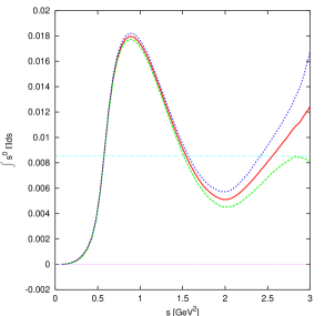
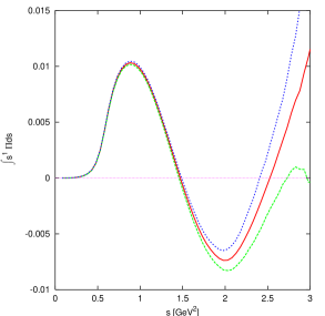
Figure 1: The first and second Weinberg sum rule as a function of the upper integration variable $s$. The central curve corresponds to the central values of [18] while the upper and lower curve are the one sigma errors calculated as described in the text.

These two sum rules are plotted in Fig. 1 for the central data values and the one sigma errors. These latter are calculated by generating a distribution of spectral functions distributed according to the covariance matrix of [18]. We then take the one sigma error to be the value where 68% of the distributions fall within. All errors in the numbers of this section and in the plots shown are calculated in this way.

At this point, we would like to discuss where local duality sets in: $s_{0}$. As we can see from Fig. 1 for $s<M_{\tau}^{2}$ there are two points where (6) are satisfied, the first one around 1.5 GeV² and the second around 2.5 GeV². Of course, this does not mean that local duality is already settled at these points as the oscillations show. One can expect however that the violations of local duality are small at these points. It is also obvious that local duality will be better when the value of $s_{0}$ is larger. The procedure to determine the value of $s_{0}$ is repeated for each of the spectral functions generated before and we use consistently a spectral function together with its value of the onset of local duality.

There are several points worth making. Though for every distribution the first duality point in the 1st WSR is very near the corresponding one of the 2nd WSR, they differ by more than their error. Numerically, when used in other sum-rules they produce results outside the naive error. The second duality point, $s_{0}\approx 2.5$ GeV² yields more stable results. There is no a priori reason for the value of $s_{0}$ to be exactly the same for different sum rules.

Though the change from the 1st WSR to the second is small, and even smaller if one looks at negative moments, when one uses large positive moments (the ones we need here), the deviations are quite sizable as we will show. This is because positive large moments weigh more the higher energy region and the negative moments essentially use only information of the low energy region.

Probably in the second duality point, local duality has not been reached either but certainly we should be closer to the asymptotic regime. We therefore take the highest global duality point available, the solution of Eq. (6), around $2.5~{}$GeV². Fortunately, for the physical matrix elements, the additional $\log(t/\mu^{2})$ in the integrand reduces the contribution of the data points near the real axis for $t$ around $\mu^{2}$. This makes these sum rules much more reliable than the single moments used in [4, 5].

The second, and highest value with good data, value of $s_{0}$ where the WSRs are satisfied runs roughly between 2.2 GeV² and 3.0 GeV². But not all of these values are equally probable. If we look at the distribution of the $s_{0}$ values, there is a clear peak situated around the value calculated with the central data points but there are tails towards higher $s_{0}$. The widths of the peak are essentially the same as the errors we quote. The $s_{0}$ where the second WSR are mainly in the area

$$s_{0} = (2.53^{+0.13}_{-0.12})\,{\rm GeV}^{2}~{}\mbox{(ALEPH)}\,,\quad\quad s_{0}=(2.49^{+0.17}_{-0.13})\,{\rm GeV}^{2}~{}\mbox{(OPAL)}\,.$$ (56)

and where the first WSR is satisfied in

$$s_{0} = (2.56^{+0.15}_{-0.14})\,{\rm GeV}^{2}~{}\mbox{(ALEPH)}\,,\quad\quad s_{0}=(2.53^{+0.17}_{-0.12})\,{\rm GeV}^{2}~{}\mbox{(OPAL)}\,.$$ (57)

These errors have been obtained as explained above. In the analysis below we use all experimental distributions with their associated value of $s_{0}$ and not only those with $s_{0}$ in the intervals above.

The OPE of the $\Pi_{LR}^{T}(Q^{2})$ was studied using the same data[18] in [28]. They obtained a quite precise determination of the dimension six and eight higher dimensional operators from a fit to different moments of the energy distribution. This procedure has in principle smaller errors since one can use the tau decay kinematic factors which suppresses the data near the real axis but has a different local duality error. They use $M_{\tau}^{2}$ as upper limit of the hadronic moments, we agree with [29] that one should use the $s_{0}$ where there is global duality with QCD to eliminate possible effects of the lack of local duality at $M_{\tau}^{2}$. Another comment is that as noticed in [6] the $\alpha_{S}^{2}$ corrections used in [28] are in a different scheme [7]. These corrections in the scheme used in [17] are presented in the appendices.

We can determine the following higher dimensional operator contributions (23)

$$M_{2} \equiv \int_{0}^{s_{0}}{\rm d}t\,t^{2}\,\frac{1}{\pi}\,\mbox{Im }\Pi_{LR}^{T}(t)$$

$$= {\displaystyle\displaystyle\sum_{m=0}^{\infty}\,\sum_{i=1}}\langle 0|O^{(i)}_{2(m+3)}(0)|0\rangle(s_{0})\,(-1)^{m}\,\frac{1}{2\pi i}\,\oint_{C_{s_{0}}}\,{\rm d}s\,\frac{C^{(i)}_{2(m+3)}(s_{0},-s)}{s^{1+m}}\,$$

$$M_{3} \equiv \int_{0}^{s_{0}}{\rm d}t\,t^{3}\,\frac{1}{\pi}\,\mbox{Im }\Pi_{LR}^{T}(t)$$ (58)

$$= {\displaystyle\displaystyle\sum_{m=0}^{\infty}\,\sum_{i=1}}\langle 0|O^{(i)}_{2(m+3)}(0)|0\rangle(s_{0})\,(-1)^{m}\,\frac{1}{2\pi i}\,\oint_{C_{s_{0}}}\,{\rm d}s\,\frac{C^{(i)}_{2(m+3)}(s_{0},-s)}{s^{m}}\,.$$

In Fig. 2 we have plotted the value of $M_{2}$ and $M_{3}$ as a function of $s_{0}$ used in the integration, together with the one sigma error band. It is immediately obvious that the main uncertainty is the choice of $s_{0}$ to be used. This uncertainty is increasingly important with the increase of the moment.

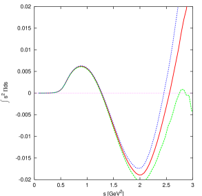
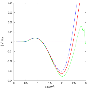
Figure 2: The second and third moment as a function of the upper limit of integration $s_{0}$ and the one sigma variation.

Using ALEPH data on $V-A$ spectral functions we get for the dimension six and eight FESR using the value for $s_{0}$ where the second WSR is satisfied

$$M_{2} = -(1.7^{+1.2}_{-1.0})\cdot 10^{-3}\,{\rm GeV}^{6}$$

$$M_{3} = (7.2^{+5.2}_{-4.0})\cdot 10^{-3}\,{\rm GeV}^{8}\,.$$ (59)

The error bars are obtained by taking 68% of the generated distributions within this value, only including those where the WSR can be satisfied. The error is smaller than one would judge from Fig. 2 since the value of $M_{2}$ and $M_{3}$ at the value of $s_{0}$ where the spectral function satisfies a WSR is much more stable than the variation at a fixed value of $s_{0}$.

Using the OPAL data we get,

$$M_{2} = -(2.0^{+1.0}_{-1.0})\cdot 10^{-3}\,{\rm GeV}^{6}$$

$$M_{3} = (5.2^{+4.0}_{-3.2})\cdot 10^{-3}\,{\rm GeV}^{8}\,.$$ (60)

Eq. (6) and (6) should be compared to the results in [18, 19, 28]

$$M_{2} = -(3.2\pm 0.9)\cdot 10^{-3}\,{\rm GeV}^{6}$$

$$M_{3} = -(4.4\pm 1.2)\cdot 10^{-3}\,{\rm GeV}^{8}\,.$$ (61)

The result for $M_{2}$ is compatible within errors but $M_{3}$ differs even in sign. Our error bars take into account the variation of $s_{0}$ but our result for $M_{3}$ at the second duality point is always positive.

This indicates a potential problem in the determination of $M_{3}$ and higher moments (and of smaller importance in $M_{2}$). As said before violations of local duality can be sizeable for higher moments like $M_{3}$ even at $t\simeq M_{\tau}^{2}$ used as upper limit of the moment integrals. It would very helpful to do the same type of fit analysis done in [28] but using the duality point $s_{0}$. Our conclusion is that moments like $M_{2}$, $M_{3}$ and higher are unfortunately unreliable unless one has data at higher energies.

The integrals which are needed for Eq. (45) can be evaluated from the ALEPH data in the same way. We need

$${\cal A}_{LR}(\mu_{R}) \equiv {\displaystyle\int^{s_{0}}_{0}}\,{\rm d}t\,t^{2}\ln\left(\frac{t}{\mu_{R}^{2}}\right)\,\frac{1}{\pi}\,\mbox{Im }\,\Pi_{LR}^{T}(t)=(4.7_{-0.4}^{+0.5})\cdot 10^{-3}~{}{\rm GeV}^{6}\,;$$

$${\cal A}^{\rm Lower}_{LR}(\mu_{R}) \equiv -{\displaystyle\int^{s_{0}}_{0}}\,{\rm d}t\,t^{2}\ln\left(1+\frac{\mu_{R}^{2}}{t}\right)\,\frac{1}{\pi}\,\mbox{Im }\,\Pi_{LR}^{T}(t)=(3.7_{-0.4}^{+0.5})\cdot 10^{-3}~{}{\rm GeV}^{6}\,;$$

$${\cal A}^{\rm Higher}_{LR}(\mu_{R}) \equiv {\displaystyle\int^{s_{0}}_{0}}\,{\rm d}t\,t^{2}\ln\left(1+\frac{t}{\mu_{R}^{2}}\right)\,\frac{1}{\pi}\,\mbox{Im }\,\Pi_{LR}^{T}(t)=(1.0_{-0.7}^{+0.9})\cdot 10^{-3}~{}{\rm GeV}^{6}$$ (62)

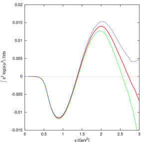
Figure 3: The integral over the spectral function needed for $\mbox{Im }G_{E}$.

at $\mu_{R}$ = 2 GeV and using for each distribution its second duality point $s_{0}$. Notice the much smaller error of ${\cal A}_{LR}$ and ${\cal A}^{\rm Lower}_{LR}$ when compared with $M_{2}$ and $M_{3}$. These values are all taken at the second duality point $s_{0}$ where the second WSR is satisfied. We plot ${\cal A}_{LR}$ as a function of $s_{0}$ in Fig. 3. The OPAL data give instead

$${\cal A}_{LR}(\mu_{R}) = (4.4_{-0.3}^{+0.4})\cdot 10^{-3}~{}{\rm GeV}^{6}\,;$$

$${\cal A}^{\rm Lower}_{LR}(\mu_{R}) = (3.8_{-0.5}^{+0.4})\cdot 10^{-3}~{}{\rm GeV}^{6}\,;$$

$${\cal A}^{\rm Higher}_{LR}(\mu_{R}) = (0.6_{-0.6}^{+0.8})\cdot 10^{-3}~{}{\rm GeV}^{6}$$

As a test, we can also calculate the electromagnetic pion mass difference in the chiral limit [31],

$${\cal B}_{LR} = {\displaystyle\int^{s_{0}}_{0}}\,{\rm d}t\,t\,\ln\left(\frac{t}{\mu_{R}^{2}}\right)\,\frac{1}{\pi}\,\mbox{Im }\,\Pi_{LR}^{T}(t)=\frac{4\pi F_{0}^{2}}{3\alpha_{QED}}\,\left(m_{\pi^{0}}^{2}-m_{\pi^{+}}^{2}\right)$$ (64)

$$= -(5.2\pm 0.5)\cdot 10^{-3}~{}{\rm GeV}^{4}~{}\mbox{(ALEPH)}\,;$$

$$= -(5.2\pm 0.6)\cdot 10^{-3}~{}{\rm GeV}^{4}~{}\mbox{(OPAL)}\,;$$

where we also used the value of $s_{0}$ given by the 2nd WSR. Notice that ${\cal B}_{LR}$ does not depend on $\mu_{R}$ due to the second WSR (6). The experimental number is

$$\frac{4\pi F_{0}^{2}}{3\alpha_{QED}}\,\left(m_{\pi^{0}}^{2}-m_{\pi^{+}}^{2}\right)_{\rm E.M.} = -(5.15\pm 0.90)\cdot 10^{-3}\,{\rm GeV}^{4}\,.$$ (65)

where we used $F_{0}=(87\pm 6)$ MeV as the chiral limit value of the pion decay constant and removed the QCD contributions [32].

For comparison we quote the central values using as $s_{0}$ the second duality point where the first WSR is satisfied

$$\begin{array}[]{rclrcl}s_{0}&=&(2.56^{+0.15}_{-0.14})~{}\mbox{GeV}^{2}\,,&{\cal A}_{LR}(2{\rm GeV})&=&(4.0_{-0.7}^{+0.6})\cdot 10^{-3}\,{\rm GeV}^{6}\,,\\ M_{2}&=&-(0.1_{-2.8}^{+3.0})\cdot 10^{-3}\,{\rm GeV}^{6},&{\cal A}^{Lower}_{LR}(2{\rm GeV})&=&(2.2\pm 2.1)\cdot 10^{-3}\,{\rm GeV}^{6},\\ M_{3}&=&(11_{-7}^{+9})\cdot 10^{-3}\,{\rm GeV}^{8}\,,&{\cal A}^{Higher}_{LR}(2{\rm GeV})&=&(1.8_{-1.6}^{+0.5})\cdot 10^{-3}\,{\rm GeV}^{6}.\end{array}$$ (69)

for ALEPH and for OPAL

$$\begin{array}[]{rclrcl}s_{0}&=&(2.53^{+0.17}_{-0.12})~{}\mbox{GeV}^{2}\,,&{\cal A}_{LR}(2{\rm GeV})&=&(3.4_{-0.8}^{+0.7})\cdot 10^{-3}\,{\rm GeV}^{6}\,,\\ M_{2}&=&(0.1_{-2.3}^{+2.8})\cdot 10^{-3}\,{\rm GeV}^{6},&{\cal A}^{Lower}_{LR}(2{\rm GeV})&=&(1.7^{+1.4}_{-1.3})\cdot 10^{-3}\,{\rm GeV}^{6},\\ M_{3}&=&(10_{-6}^{+9})\cdot 10^{-3}\,{\rm GeV}^{8}\,,&{\cal A}^{Higher}_{LR}(2{\rm GeV})&=&(1.7_{-1.3}^{+1.8})\cdot 10^{-3}\,{\rm GeV}^{6}.\end{array}$$ (73)

The errors are larger here. The value of $s_{0}$ where the first WSR is satisfied varies more and is somewhat larger than the $s_{0}$ where the second WSR is satisfied, this makes the last results more dependent on the spectral function at high $t$ which have large errors.

If one tried to see the results using the first duality point, where less duality with QCD is expected, we get that using the one from the 2nd WSR

$$\begin{array}[]{rclrcl}s_{0}&=&(1.47\pm 0.02)\,{\rm GeV}^{2}\;,&{\cal A}_{LR}(2{\rm GeV})&=&(3.3\pm 0.1)\cdot 10^{-3}\,{\rm GeV}^{6},\\ M_{2}&=&-(6.6\pm 0.2)\cdot 10^{-3}\,{\rm GeV}^{6},&{\cal A}^{Lower}_{LR}(2{\rm GeV})&=&(5.9\pm 0.2)\cdot 10^{-3}\,{\rm GeV}^{6},\\ M_{3}&=&-(12_{-2}^{+1})\cdot 10^{-3}\,{\rm GeV}^{8},&{\cal A}^{Higher}_{LR}(2{\rm GeV})&=&-(2.6\pm 0.1)\,{\rm GeV}^{6}.\end{array}$$ (77)

Notice that $M_{2}$ is not compatible with (6) with the central values differing by more than twice the error. The moment $M_{3}$ changes even sign with respect to the second duality point showing the problems of local duality violations for larger moments more dramatically. As argued before one should the largest value of $s_{0}$ to ensure better local duality. However, the physical relevant moment ${\cal A}_{LR}$ is much more stable with $s_{0}$.

7 The Scalar–Pseudo-Scalar Two-Point Function $\Pi_{SS+PP}^{(0-3)}(Q^{2})$

In this section we discuss some of the knowledge of the spectral function $\mbox{Im }\Pi_{SS+PP}^{(0-3)}(t)$ which governs the connected contribution to the matrix element of $Q_{8}$. In the large $N_{c}$ limit there is no difference between the singlet and triplet channel so the integral in (78) is $1/N_{c}$ suppressed and its contribution to $\mbox{Im }G_{E}$ is NNLO. But in the scalar-pseudo-scalar sector, violations of the large $N_{c}$ behaviour can be larger than in the vector-axial-vector channel. It is therefore interesting to determine the size of this contribution as well.

After adding the short-distance part to the long-distance part, the relevant integral is (45)

$$\,\frac{1}{48\pi^{2}}\frac{1}{\langle 0|\bar{q}q|0\rangle^{2}(\mu_{C})}\,\int_{0}^{\tilde{s}_{0}}{\rm d}t\,t\,\ln\left(\frac{t}{\mu^{2}}\right)\,\frac{1}{\pi}\,\mbox{Im }\Pi_{SS+PP}^{(0-3)}(t)\,,$$ (78)

This is the contribution of the connected part relative to the disconnected one. $\tilde{s}_{0}$ is the scale where in this channel QCD duality sets in. The scale $\mu$ is the cut-off scale. The dependence on this scale being NNLO in $1/N_{c}$ cannot match the present NLO order Wilson coefficients.

We can use models like the ones in [26] to evaluate the scalar part of the integrals. We only use the model there using the KLM[33] analysis, since only it ratifies (37) at a reasonable value of $\tilde{s}_{0}$. In Fig. 4 we plotted for that parameterization the sum rule and the relative correction from the scalar part to the disconnected contribution $3\langle 0|\overline{q}q|0\rangle^{2}(\mu_{R})$ for $\mu=\mu_{R}=2$ GeV.

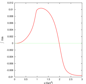
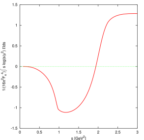
Figure 4: The sum rule (37) as a function of $\tilde{s}_{0}$ for the scalar part and the relative correction to the disconnected contribution for $Q_{8}$ using the same parametrization as a function of $\tilde{s}_{0}$ for $\mu_{R}=\mu=$ 2 GeV. Notice that the correction is small in the region where the sum rule is satisfied.

The value of the scalar part of Eq. (78) is about 0.18 at $\tilde{s}_{0}=(1.41$ GeV)².

In the large $N_{c}$ limit, a sensible alternative estimate is to use meson pole dominance. In the pseudo-scalar sector, the U(3)$\times$U(3) symmetry is broken by the chiral anomaly splitting the singlet $\eta_{1}$ mass away from the zero mass for the Goldstone boson octet.

Three meson intermediate states are not studied enough to be included at this level, we include instead the first $\pi^{\prime}$ resonance. This means including a massless Goldstone boson plus the first $\pi^{\prime}$ resonance and the singlet $\eta_{1}$. The pseudo-scalar sum rule in (37) requires the following relation between the octet and the singlet couplings to the pseudo-scalar current for $\tilde{s}_{0}\simeq 2.0$ GeV²,

$$F_{0}^{2}+F_{\pi^{\prime}}^{2}=F_{\eta_{1}}^{2}\,.$$ (79)

Phenomenologically $F_{\pi^{\prime}}^{2}/F_{0}^{2}<<1$ [34] and $F_{0}\simeq F_{\eta_{1}}$.

We can introduce a scalar meson octet $S_{8}$ and a singlet $S_{1}$ using the methods of [35]. The coupling constant for the octet can be denoted by $c_{m}$ and has been estimated in [35, 36] to be about $(43\pm 14)$ MeV. In fact, the sum rule (35) is a property of QCD and relates in this approximation $c_{m}$ to $F_{0}$

$$c_{m}^{2}=\frac{1}{8}\left[F_{0}^{2}+F_{\pi^{\prime}}^{2}+\cdots\right]=\frac{F_{\eta_{1}}^{2}}{8}\simeq\frac{F_{0}^{2}}{8}$$ (80)

which numerically agrees quite well with the phenomenological estimate.

The scalar sum rule in (37) requires the singlet and the octet components to have the same coupling leading to a relative correction from the scalar integral to the disconnected contribution of

$$\frac{1}{12\pi^{2}}\frac{F_{\eta_{1}}^{2}}{F_{0}^{4}}\,\left[M_{S_{1}}^{2}\ln\left(\frac{M_{S_{1}}}{\mu}\right)-M_{S_{8}}^{2}\ln\left(\frac{M_{S_{8}}}{\mu}\right)\right].$$ (81)

using both sum rules and the lowest meson dominance approximation.

The contribution from the pseudo-scalar connected two-point function relative the disconnected contribution can then be evaluated to

$$\frac{1}{12\pi^{2}}\frac{F_{\eta_{1}}^{2}}{F_{0}^{4}}\,\left[M_{\eta_{1}}^{2}\,\ln\left(\frac{M_{\eta_{1}}}{\mu}\right)\,-\frac{F_{\pi^{\prime}}^{2}}{F_{\eta_{1}}^{2}}\,M_{\pi^{\prime}}^{2}\ln\left(\frac{M_{\pi^{\prime}}}{\mu}\right)\right]\,.$$ (82)

The contribution of the $\pi^{\prime}$ is negligible.

As said before the scale $\mu$ is free and cannot be at present matched with OPE QCD since it is a NNLO order in $1/N_{c}$ effect. The scale independence is reached when the sum rule

$$\tilde{M}_{1} = M_{S_{8}}^{2}-M_{S_{1}}^{2}-M_{\eta_{1}}^{2}+\frac{F_{\pi^{\prime}}^{2}}{F_{\eta_{1}}^{2}}M_{\pi^{\prime}}^{2}=0$$ (83)

which is $O(N_{c}^{2}\alpha^{2})$ (4.2) is fulfilled. This sum rule is very well satisfied in the linear $\sigma$ model, see e.g. [26].

The masses $M_{\eta_{1}}\simeq 0.86$ GeV (chiral limit value) $M_{\pi^{\prime}}\simeq 1.3$ GeV are known. The masses of the singlet and octet of scalars are not so well known. Using $M_{S_{1}}=M_{\sigma}\simeq 0.5$ GeV and $M_{S_{8}}=M_{a_{0}(980)}\simeq 0.98$ GeV the correction to the disconnected contribution is almost independent of the scale $\mu$, neglecting the $\pi^{\prime}$ and is independent of $\mu$ for $F_{\pi^{\prime}}^{2}/F_{0}^{2}=0.017$. The relative scalar contribution is about $0.40$ and the relative pseudoscalar is $-0.71$ with a total relative contribution of about $-0.31$. The scalar contribution is within errors compatible with the earlier estimate.

From the discussion here it can be seen that there is a possibly sizable correction but we expect it to be smaller than $-40$%.

Of course, the scale dependence left in (78) is unsatisfactory in principle but small since the sum rule (83) is quite well satisfied.

8 Numerical Results for the Matrix-Elements and Bag Parameters

The vacuum expectation value in the chiral limit of $Q_{7}$ itself is related directly to $B_{7\chi}$. This allows us to obtain

$$\langle 0|O_{6}^{(1)}(0)|0\rangle^{NDR}(\mu_{R}) = -\left(1+\frac{1}{24}a(\mu_{R})\right)\,\frac{3}{32\pi^{2}}{\cal A}_{LR}(\mu_{R})$$ (84)

$$+ \frac{1}{48}\,a(\mu_{R})\,\left[3\langle 0|\overline{q}q|0\rangle^{2}(\mu_{R})+\frac{1}{16\pi^{2}}{\cal A}_{SP}(\mu_{R},\mu_{C})\right]\,;$$

$$\langle 0|O_{6}^{(1)}(0)|0\rangle^{HV}(\mu_{R}) = -\left(1-\frac{11}{24}a(\mu_{R})\right)\frac{3}{32\pi^{2}}\,{\cal A}_{LR}(\mu_{R})$$ (85)

$$- \frac{11}{48}\,a(\mu_{R})\,\left[3\langle 0|\overline{q}q|0\rangle^{2}(\mu_{R})\,+\frac{1}{16\pi^{2}}{\cal A}_{SP}(\mu_{R},\mu_{C})\right]\,.$$

For the numerics, we use the value of the condensate obtained in the $\overline{MS}$ scheme in [37],

$$\langle 0|\overline{q}q|0\rangle(2{\rm GeV}) = -(0.018\pm 0.004)\,{\rm GeV}^{3}\,,$$ (86)

the numerical results of Eq. (6),

$$a(2~{}GeV)=0.102$$ (87)

and neglect, in first approximation, the integral over the scalar–pseudo-scalar two-point function.

The weighted average of the first and second WSR results for ${\cal A}_{LR}(2{\rm GeV})$ from ALEPH data is

$${\cal A}^{\rm ALEPH}_{LR}(2{\rm GeV})=(4.5\pm 0.5)\cdot 10^{-3}~{}{\rm GeV}^{6}$$ (88)

and from OPAL data

$${\cal A}^{\rm OPAL}_{LR}(2{\rm GeV})=(4.2\pm 0.4)\cdot 10^{-3}~{}{\rm GeV}^{6}\,.$$ (89)

Though the systematic errors aver very correlated, sicne the central values are very similar we take the simple average of both results as our result

$${\cal A}_{LR}(2{\rm GeV})=(4.35\pm 0.50)\cdot 10^{-3}~{}{\rm GeV}^{6}\,$$ (90)

and obtain

$$\langle 0|O_{6}^{(1)}(0)|0\rangle^{NDR}(2{\rm GeV})=-(4.0\pm 0.5)\cdot 10^{-5}~{}{\rm GeV}^{6}$$ (91)

$$= \left(-(4.2\pm 0.5)+(0.2\pm 0.1)\right)\cdot 10^{-5}~{}{\rm GeV}^{6}$$

$$= \left((-3.3\pm 0.5)+(-0.9\pm 0.8)+(0.2\pm 0.1)\right)\cdot 10^{-5}~{}{\rm GeV}^{6}$$

and

$$\langle 0|O_{6}^{(1)}(0)|0\rangle^{HV}(2{\rm GeV})=-(6.2\pm 1.0)\cdot 10^{-5}~{}{\rm GeV}^{6}$$ (92)

$$= \left((-3.9\pm 0.5)-(2.3\pm 0.9)\right)\cdot 10^{-5}~{}{\rm GeV}^{6}$$

$$= \left((-3.1\pm 0.5)+(-0.8\pm 0.7)-(2.3\pm 0.9)\right)\cdot 10^{-5}~{}{\rm GeV}^{6}$$

where we quote, namely, the total result, the integral and the vacuum expectation value separately and in the last case also the long and short-distance part of the integral separately.

The short-distance part of the integral, the second term in the above, is the contribution of all higher dimensional operators. We find that its contribution is between a few % up to 35 % depending on the value of $\mu$. At $\mu=2$ GeV it is somewhat larger than the error on the integral cut-off at $\mu$.

Similarly, the matrix-element of $Q_{8}$ is directly related to $B_{8}$ and we obtain

$$\langle 0|O_{6}^{(2)}(0)|0\rangle^{NDR}(2{\rm GeV}) = \left[1+\frac{23}{12}\,a(2{\rm GeV})\right]\times$$ (93)

$$\times\left[3\,\langle 0|\overline{q}q|0\rangle^{2}(2{\rm GeV})+\frac{1}{16\pi^{2}}{\cal A}_{SP}(2\rm{GeV},2\rm{GeV})\right]\,$$

$$- \frac{27}{64\pi^{2}}\,a(2{\rm GeV})\,{\cal A}_{LR}(2{\rm GeV})\,.$$

$$\langle 0|O_{6}^{(2)}(0)|0\rangle^{HV}(2{\rm GeV}) = \left[1+\frac{35}{12}\,a(2{\rm GeV})\right]\times$$ (94)

$$\times\left[3\,\langle 0|\overline{q}q|0\rangle^{2}(2{\rm GeV})+\frac{1}{16\pi^{2}}{\cal A}_{SP}(2\rm{GeV},2\rm{GeV})\right]\,$$

$$+ \frac{9}{64\pi^{2}}\,a(2{\rm GeV})\,{\cal A}_{LR}(2{\rm GeV})\,.$$

Using the same input as above we obtain

$$\langle 0|O_{6}^{(2)}(0)|0\rangle^{NDR}(2{\rm GeV}) = (1.2\pm 0.5)\cdot 10^{-3}\,{\rm GeV}^{6}\,,$$

$$\langle 0|O_{6}^{(2)}(0)|0\rangle^{HV}(2{\rm GeV}) = (1.3\pm 0.6)\cdot 10^{-3}\,{\rm GeV}^{6}\,,$$ (95)

where the contribution of the integral over $\mbox{Im }\Pi_{LR}^{T}$ is at the 1% level and thus totally negligible.

Another combination of these two matrix-elements can also be obtained from an integral over the ALEPH data[9, 17] by putting (4.1.2) and (23) in (6) including also the $\alpha_{S}$ correction of the appendix :

$$M_{2} = \int_{0}^{s_{0}}{\rm d}t\,t^{2}\,\frac{1}{\pi}\,\mbox{Im }\Pi_{LR}^{T}(t)={\displaystyle\sum_{i=1}}\,C^{(i)}_{6}(s_{0},s_{0})\,O^{(i)}_{6}(s_{0})$$ (96)

$$= -\frac{4\pi^{2}}{3}\,a(s_{0})\left[2\left(1+\frac{13}{8}\,a(s_{0})\right)\,\langle 0|O_{6}^{(1)}(0)|0\rangle^{NDR}(s_{0})\right.$$

$$+ \left.\,\left(1+\frac{25}{8}a(s_{0})\right)\,\langle 0|O_{6}^{(2)}(0)|0\rangle^{NDR}(s_{0})\right]\,$$

$$= -\frac{4\pi^{2}}{3}\,a(s_{0})\left[2\left(1+\frac{41}{8}\,a(s_{0})\right)\,\langle 0|O_{6}^{(1)}(0)|0\rangle^{HV}(s_{0})\right.$$

$$+ \left.\,\left(1+\frac{21}{8}a(s_{0})\right)\,\langle 0|O_{6}^{(2)}(0)|0\rangle^{HV}(s_{0})\right]\,.$$

$$= -4\pi^{2}a(s_{0})\left[\left(1+\frac{61}{12}a(s_{0})\right)\,\left[\langle 0|\overline{q}q|0\rangle^{2}(s_{0})+\frac{1}{48\pi^{2}}{\cal A}_{SP}(s_{0},s_{0})\right]\,\right.$$

$$- \left.\left(1+\frac{47}{12}a(s_{0})\right)\frac{1}{16\pi^{2}}{\cal A}_{LR}(s_{0})\right]$$

The right hand-side is physical and we cheked that is independent of the scale $s_{0}$ and scheme. We can therefore evaluate it at $s_{0}=4$ GeV². The contribution from $\langle 0|O_{6}^{(1)}(0)|0\rangle^{NDR}(s_{0})$ is numerically very small and we obtain

$$M_{2}=-(2.0\pm 0.9)\cdot 10^{-3}~{}\mbox{GeV}^{6}\,,$$ (97)

perfectly compatible within errors both with the result obtained from the data in Eq. (6) and with the result (6). This confirms our results on the size of the integral over $\mbox{Im }\Pi_{SS+PP}(t)$, which can therefore be considered negligible within the present accuracy of the disconnected contribution and $M_{2}$.

There is another sum rule which combines the two matrix elements,

$$\tilde{M}_{1} = \int_{0}^{\tilde{s}_{0}}{\rm d}t\,t\,\frac{1}{\pi}\,\mbox{Im }\Pi_{SS+PP}(t)=-{\displaystyle\sum_{i=1}}\,\tilde{C}^{(i)}_{6}(s_{0},s_{0})\,O^{(i)}_{6}(s_{0})$$

$$= -\frac{\pi^{2}}{4}\,a(s_{0})^{2}\,\left[211\,\langle 0|O_{6}^{(2)}(0)|0\rangle(\tilde{s}_{0})+90\,\langle 0|O_{6}^{(1)}(0)|0\rangle(\tilde{s}_{0})\right]+O(a^{3})\,.$$

For the calculation of the coefficients see Appendix B. This sum rule is much less accurate than $M_{2}$ since the leading terms are $\alpha_{S}^{2}$ and the value of $\tilde{M}_{1}$ is not known directly either. Therefore we don’t use it.

The numerical estimates of the disconnected part, ${\cal A}_{SP}$, given above change these numbers somewhat but within the errors quoted.

These results can also be expressed in terms of the bag parameters:

$$B_{7\chi}^{NDR}(2{\rm GeV}) = 0.75\pm 0.20\;;\quad B_{7\chi}^{HV}(2{\rm GeV})=1.15\pm 0.30\;$$

$$B_{8\chi}^{NDR}(2{\rm GeV}) = 1.2\pm 0.3\;;\quad B_{8\chi}^{HV}(2{\rm GeV})=1.3\pm 0.4\,.$$ (99)

We can also express it in terms of $\mbox{Im }G_{E}$:

$$F_{0}^{6}~{}\mbox{Im }G_{E} = \mbox{Im }\tau(-2.1\pm 0.9)~{}10^{-6}~{}\mbox{GeV}^{6}\,$$ (100)

which is quite compatible with the estimate in [12].

9 Comparison with earlier results

To compare with other results in the literature we propose to use the VEVs $\langle 0|O_{6}^{1)}|0\rangle$ and $\langle 0|O_{6}^{(2)}|0\rangle$. The reason is that these quantities are what [4, 5, 6] and we directly compute. The matrix elements of $K\to\pi\pi$ through $Q_{7}$ and $Q_{8}$, in the chiral limit, can be expressed as follows [12]

$$M_{2}[Q_{7}](\mu_{R}) = \langle(\pi\pi)_{I=2}|Q_{7}|K^{0}\rangle(\mu_{R})=-\sqrt{\frac{2}{3}}\,\frac{\langle 0|\overline{q}q|0\rangle^{2}(\mu_{C})}{F_{0}^{3}}\,\,B_{7\chi}(\mu_{C},\mu_{R})\,$$

$$= 2\sqrt{6}\,\frac{\langle 0|O_{6}^{(1)}|0\rangle_{\chi}(\mu_{R})}{F_{0}^{3}}\,;$$

$$M_{2}[Q_{8}](\mu_{R}) = \langle(\pi\pi)_{I=2}|Q_{8}|K^{0}\rangle(\mu_{R})=-\sqrt{6}\,\frac{\langle 0|\overline{q}q|0\rangle^{2}(\mu_{C})}{F_{0}^{3}}\,\,B_{8\chi}(\mu_{C},\mu_{R})\,$$ (101)

$$= -\frac{\sqrt{6}}{3}\,\frac{\langle 0|O_{6}^{(2)}|0\rangle_{\chi}(\mu_{R})}{F_{0}^{3}}\,.$$

The lattice results[38] are from computed $K\to\pi$ matrix elements and use the physical values of $f_{K}$ and $f_{\pi}$ to convert into $K\to\pi\pi$. Since we and [4, 5, 6] compute in the chiral limit, this amounts to a large spurious factor $f_{K}f_{\pi}^{2}/F_{0}^{3}\simeq 1.6$ of difference when comparing $K\to\pi\pi$ matrix elements or $f_{K}f_{\pi}/F_{0}^{2}\simeq 1.4$ when comparing $K\to\pi$ matrix elements. Usually this factor is not taken into account. Moreover each group uses different conventions, either the chiral limit value of $f_{\pi}$ and $f_{K}$ or their physical value. We give the lattice results for $K\to\pi$ rescaling with the factor above.

Reference	$-10^{5}\langle 0|O_{6}^{(1)}|0\rangle^{NDR}_{\chi}\,{\rm GeV}^{-6}$	$10^{3}\langle 0|O_{6}^{(2)}|0\rangle^{NDR}_{\chi}\,{\rm GeV}^{-6}$
$B_{7}=B_{8}=1$	$5.4\pm 2.2$	$1.0\pm 0.4$
This work (SS+PP=0)	$4.0\pm 0.5$	$1.2\pm 0.5$
Knecht et al. [6]	$1.9\pm 0.6$	$3.5\pm 1.1$
Cirigliano et al. [39]	$2.7\pm 1.7$	$2.2\pm 0.7$
Donoghue et al.[4]	$4.3\pm 0.9$	$1.5\pm 0.4$
Narison [5]	$3.5\pm 1.0$	$1.5\pm 0.3$
lattice [38]	$2.6\pm 0.7$	$0.74\pm 0.15$
ENJL [12]	$4.3\pm 0.5$	$1.3\pm 0.2$

Table 1: The values of the VEVs in the NDR scheme at $\mu_{R}=2$ GeV.

Reference	$-10^{5}\langle 0|O_{6}^{(1)}|0\rangle^{HV}_{\chi}\,{\rm GeV}^{-6}$	$10^{3}\langle 0|O_{6}^{(2)}|0\rangle^{HV}_{\chi}\,{\rm GeV}^{-6}$
$B_{7}=B_{8}=1$	$5.4\pm 2.2$	$1.0\pm 0.4$
This work (SS+PP=0)	$6.2\pm 1.0$	$1.3\pm 0.6$
Knecht et al. [6]	$11.0\pm 2.0$	$3.5\pm 1.1$
Cirigilano et al.[39]	$8.2\pm 0.9$	$2.4\pm 0.7$
lattice [38]	$4.3\pm 1.1$	$0.8\pm 0.2$
ENJL [12]	$7.1\pm 0.9$	$1.4\pm 0.2$

Table 2: The values of the VEVs in the HV scheme at $\mu_{R}=2$ GeV.

We agree with the old results by [4, 8] including the higher order operators. In fact, they also make an estimate of their contribution which agrees with our full calculation. We also agree reasonably well with [5]. We agree borderline with their new results[39] within errors, though their central value is almost twice ours for $Q_{8}$.

We do not agree with [6] even within errors. But if the $O(a^{2})$ correction in (96) is taken into account, their result for $O_{6}^{(2)}$ goes to $(2.7\pm 0.9)\,10^{-3}$ and we are borderline also within errors though the central value is more than twice ours.

We find a systematic a factor around 1.5 to 1.8 compared lattice results[38] for both matrix elements. They are compatible when we take the errors on both the lattice and our results into account and the fact that the lattice numbers are not in the chiral limit. The corrections for the latter we included only partially with the physical values of $f_{K}$ and $f_{\pi}$.

We have not quoted the results from the CHPT large $N_{c}$ approach[40] and the chiral quark model [41] because they are away from the chiral limit.

Our results are very compatible with our earlier work. In [12] we used the ENJL model and a very low value of $\mu$ to estimate the same matrix-elements. The underlying reason for the agreement is that the operators $Q_{7}$ and $Q_{8}$ mix quite strongly and the values of the matrix-element of $Q_{8}$ at the low scale $\mu\approx 0.8$ GeV dominate the values of the matrix-elements of $Q_{7}$ and $Q_{8}$ at the higher scale $\mu=2$ GeV. The matrix element of $Q_{8}$ obtained here is the same as the one we used in [12], since the effect of ${\cal A}_{SP}$ is estimated to be moderate here.

9.1 Rôle of Higher Dimensional Operators

We clarified here the role of the higher than six dimensional operators, an issue raised in [8]. In our scheme they remove the $\mu$-dependence which is not covered by the renormalization group.

The effect of higher dimension operators in our approach is to add ${\cal A}_{LR}^{\rm Higher}(\mu)$ to the low energy contribution ${\cal A}_{LR}^{\rm Lower}(\mu)$, these are defined in Eq. (6),

$${\cal A}_{LR}(\mu) = {\cal A}_{LR}^{\rm Higher}+{\cal A}_{LR}^{\rm Lower}=\int_{0}^{s_{0}}{\rm d}t\,t^{2}\,\ln\left(\frac{t}{\mu^{2}}\right)\,\frac{1}{\pi}\,\mbox{Im }\Pi_{LR}^{T}(t)\,$$ (102)

where $\mu$ is an Euclidean cut-off. It is clear than the contribution of higher than dimension six operators is less important only for values of $\mu^{2}$ larger than $s_{0}$, where $\mbox{Im }\Pi^{T}_{LR}$ vanishes because of local duality. In Figure 5 we plot the two separate contributions and the sum as a function of $\mu$.

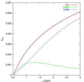
Figure 5: The separate contributions to ${\cal A}_{LR}$ and the sum. “Higher” labels the effect of the higher than six dimensional operators in the short-distance contribution and “Lower” the long-distance part.

From the figure we can see for $\mu$ larger than 2 GeV the contribution of all higher dimensional operators is less than 25 %. We agree with [8] that for the matrix elements that involve integrals of $\mbox{Im }\Pi^{T}_{LR}$ one has to go to such values of $\mu$ to disregard the contribution of higher dimensional operators. The contribution we find is somewhat smaller than in [8] since we include the effect of all higher order operators, not just dimension eight.

The high value of $\mu$ is set by the threshold of perturbative QCD $s_{0}$ which depends very much on the spectral function and on the integrand behaviour. In fact, from [42] one can see that relevant spectral function for the 27-plet coupling reaches the perturbative QCD behaviour very soon, from 0.7 GeV to 1 GeV. The OPE matched impressively well with the hadronic ansatz at such low values with just dimension six operators. Therefore though higher dimensional operators appear one can expect smaller contributions in cases like $G_{27}$ and $\mbox{Re }G_{8}$.

The matrix-elements studied in this paper might be special in the sense that they follow from integrals over spectral functions which have no contributions at short-distances from the unit operator or the dimension four operators. As the good matching at low scales in the example in [42] shows, the other quantities which have these contributions might have much smaller higher dimension effects.

9.2 The Large $N_{c}$ Limit

In the large $N_{c}$ limit, the spectral functions have only poles:

$$\frac{1}{\pi}\,\mbox{Im }\Pi^{T}_{LR}(t) = -F_{0}^{2}\delta(t)-\sum_{A}^{\infty}f_{A}^{2}M_{A}^{2}\delta(t-M_{A}^{2})+\sum_{V}^{\infty}f_{V}^{2}M_{V}^{2}\delta(t-M_{V}^{2})$$ (103)

and

$$\frac{1}{\pi}\,\mbox{Im }\Pi^{(0-3)}_{SS+PP}(t) = 4\frac{\langle 0|\overline{q}q|0\rangle^{2}(\mu_{C})}{F_{0}^{4}}\,\left[8\sum_{S_{1}}^{\infty}\tilde{c}_{m,S_{1}}^{2}\delta(t-M_{S_{1}}^{2})-8\sum_{S_{8}}^{\infty}c_{m,S_{8}}^{2}\delta(t-M_{S_{8}}^{2})\right.$$ (104)

$$- \left.\sum_{\eta_{1}}^{\infty}F_{\eta_{1}}^{2}\delta(t-M_{\eta_{1}}^{2})+F_{0}^{2}\delta(t)+\sum_{\pi^{\prime}}^{\infty}F_{\pi^{\prime}}^{2}\delta(t-M_{\pi^{\prime}})\right]$$

at all values of $t$. The Weinberg-like Sum Rules, Eqs. (6),(35),(37), assuming local duality holds above $s_{0}$, impose

$${\displaystyle\sum_{V}^{M_{V}^{2}<s_{0}}}\,f_{V}^{2}\,M_{V}^{2}-{\displaystyle\sum_{A}^{M_{A}^{2}<s_{0}}}\,f_{A}^{2}\,M_{A}^{2} = F_{0}^{2}\,;$$

$${\displaystyle\sum_{V}^{M_{V}^{2}<s_{0}}}\,f_{V}^{2}\,M_{V}^{4}-{\displaystyle\sum_{A}^{M_{A}^{2}<s_{0}}}\,f_{A}^{2}\,M_{A}^{4} = 0\,.$$ (105)

$$F_{0}^{2}+{\displaystyle\sum_{\pi^{\prime}}^{M_{\pi^{\prime}}^{2}<\tilde{s}_{0}}}\,F_{\pi^{\prime}}^{2} = {\displaystyle\sum_{\eta_{1}}^{M_{\eta_{1}}^{2}<\tilde{s}_{0}}}\,F_{\eta_{1}}^{2}\,=8{\displaystyle\sum_{S_{8}}^{M_{S_{8}}^{2}<\tilde{s}_{0}}}\,c_{m,S_{8}}^{2}=8{\displaystyle\sum_{S_{1}}^{M_{S_{1}}^{2}<\tilde{s}_{0}}}\,\tilde{c}_{m,S_{1}}^{2}\,.$$ (106)

We will use the expression (103) to get one of the two relevant integrals defined in (4.3) and the EM pion mass difference in (64)

$${\cal A}_{LR}^{N_{c}}(\mu_{R}) = 2{\displaystyle\sum_{V}^{M_{V}^{2}<s_{0}}}\,f_{V}^{2}\,M_{V}^{6}\ln\left(\frac{M_{V}}{\mu_{R}}\right)-2{\displaystyle\sum_{A}^{M_{A}^{2}<s_{0}}}\,f_{A}^{2}\,M_{A}^{6}\ln\left(\frac{M_{A}}{\mu_{R}}\right)\,;$$

$${\cal B}_{LR}^{N_{c}} = 2{\displaystyle\sum_{V}^{M_{V}^{2}<s_{0}}}\,f_{V}^{2}\,M_{V}^{4}\ln\left(\frac{M_{V}}{\mu_{R}}\right)-2{\displaystyle\sum_{A}^{M_{A}^{2}<s_{0}}}\,f_{A}^{2}\,M_{A}^{4}\ln\left(\frac{M_{A}}{\mu_{R}}\right)$$ (107)

We can also calculate the moments defined in (4.1.2)

$$M_{n+2}^{N_{c}} = {\displaystyle\sum_{V}^{M_{V}^{2}<s_{0}}}\,f_{V}^{2}\,M_{V}^{2(n+3)}-{\displaystyle\sum_{A}^{M_{A}^{2}<s_{0}}}\,f_{A}^{2}\,M_{A}^{2(n+3)}\,.$$ (108)

These sum rules and higher moments were studied in [29] with the MHA Ansatz. The results obtained using MHA are [29]

$$M_{2}^{\rm MHA} = -(4.8\pm 1.6)\cdot 10^{-3}\,{\rm GeV}^{6}\,,\quad M_{3}^{\rm MHA}=-(8.1\pm 2.7)\cdot 10^{-3}\,{\rm GeV}^{8}$$

$${\cal A}_{LR}^{\rm MHA}(2{\rm GeV}) = (2.8\pm 1.0)\cdot 10^{-3}\,{\rm GeV}^{6}\,,\quad{\cal B}_{LR}^{MHA}=-(5.9\pm 2.0)\,\cdot 10^{-3}\,{\rm GeV}^{4}\,.$$ (109)

for any value of $s_{0}$ larger than the 1st duality point, i.e. $s_{0}\geq 1.5$ GeV² by construction.

These should be compared with our results (6) from the second duality point or (77) from the first duality point or the fit (6)[28]. The results using the MHA Ansatz are compatible with the ones using the first duality point within one sigma.

If one uses the second duality point, the moment $M_{2}$ agrees borderline within errors but their central value is more than twice our result (6). However the physical quantiy ${\cal A}_{LR}(2{\rm GeV})$ agrees within errors with our second duality point though our central value is larger. The moment $M_{3}$ is more problematic and we find that in the second duality point it changes sign.

Also [28] obtained the values of the condensates of dimension six an eight which are proportional to $M_{2}$ and $M_{3}$ from a fit to different type of moments of the same data. The results are in Eq. (6). The moment $M_{2}$ is compatible within errors with our results using the second duality point but not with the our results using the first duality point. In particular, the moment $M_{3}$ is incompatible with both our results using the first and second duality points. This must be due to the duality violations being weighted differently in (6) as mentioned previously.

We conclude from these comparisons that for the dimension eight moment $M_{3}$, local duality at low values of $s_{0}$ starts to be a problem. As we go up in the moments we need more and more accurate information at higher energies. This affects also to $M_{2}$ .

The case of more than one resonance in each channel was analyzed in full generality in [43]. There one can find the large differences that the $\rho^{\prime}$ produces in the second, third moments, and higher moments with respect to the case of a single vector resonance in each channel.

10 Conclusions

In this work, we have calculated in a model independent way the matrix elements of the $\Delta S=1$ operators $Q_{7}$ and $Q_{8}$ in the chiral limit. We have done it to all orders in $1/N_{c}$ and NLO in $\alpha_{s}$.

The scheme dependence has been taken into account exactly at NLO using the $X$ boson method as proposed and used in [11, 12, 23]. In fact, these two operators are a submatrix of the ten by ten done in [12].

We would like to mention some issues sometimes mixed up in the literature. First, the $X$ boson method has nothing to do with using or not large $N_{c}$. It can be used without the large $N_{c}$ approximation as well, as shown again in this paper. Second, our method of treating the scheme dependence is consistent and we never mix up two different schemes, cut-off and $\overline{MS}$ schemes. We do an analytic matching between a cut-off regularization and dimensional regularization in a well-defined scheme at perturbative scales first. The finite parts arising in this matching appear in the methods using dimensional regularization to the end as well as explained in the appendix.

We obtain exact matching in an Euclidean-cut-off regularization and analytical cancellation exact of (all) infrared and UV scheme dependences.

For the contribution of higher order operators discussed in [8] and [5] we clarify how to include all higher dimensional operators and exact scheme dependence at NLO in $\alpha_{S}$ of both the $Q_{7}$ and $Q_{8}$ matrix elements. As a result we find smaller corrections due to this effects as discussed in Section 9.1. In our approach the effect of the higher order operators is to remove the remaining dependence on the Euclidean cutoff $\mu$ beyond the RGE evolution. The result of resumming all higher dimensional operators in the case of $Q_{7}$ makes its prediction much less sensitive to the choice of $s_{0}$.

As noticed in [6, 12], ${\cal A}_{SP}$ is zero in the large $N_{c}$ limit and therefore is Zweig suppressed. We find no sizeable violation of the dimension six FESR using factorization for $Q_{8}$.

We find that the moment $M_{2}$ is very sensitive to the spectral function arount 2 GeV².

Our main analytical results are the expression for the matrix-elements (45), the bag parameters (5), (5) and the expansion coefficients of the spectral functions (A.2), (A.2) and (B.2). The main numerical results are the VEVs (91),(92) and the bag parameters (8). These results are exact in the chiral limit, so we have the $\Delta I=3/2$ part of $\varepsilon^{\prime}/\varepsilon$ model independently at all orders in $1/N_{c}$. In order to reach final values all effects which vanish in the chiral limit, as final state interactions, quark-mass effects, isospin violation and long-distance electromagnetic effects still need to be included.

Appendix A Calculation of the Corrections of $\mathcal{O}(a^{2})$ to the Dimension Six Contribution to $\Pi_{LR}^{T}(Q^{2})$

A.1 Renormalization Group Analysis

We have the two-point function

$$\Pi^{\mu\nu}_{LR}(q) \equiv \frac{1}{2}\,i\int d^{D}y\,e^{iq\cdot y}\langle 0|T(L^{\mu}(y)R^{\nu}(0)^{{\dagger}})|0\rangle\equiv(q^{\mu}q^{\nu}-g^{\mu\nu}q^{2})\Pi_{LR}^{T}(q^{2})$$ (110)

$$+ q^{\mu}q^{\nu}\Pi_{LR}^{L}(q^{2})$$

The contribution of dimension six operators to $\Pi_{LR}^{T}(Q^{2})$ (where $Q^{2}=-q^{2}$) can be written in $D=4-2\epsilon$ dimensions as

$$Q^{6}\,\Pi_{LR}^{T}(Q^{2})\Big{|}_{D=6}\,\equiv\,\nu^{2\epsilon}\,\sum_{i=1,2}C_{i}(\nu,Q^{2})<O_{i}>(\nu)$$ (111)

with

$$<O_{1}> \equiv \langle 0|O_{6}^{(1)}|0\rangle=\frac{1}{4}\,<0|(\overline{s}\gamma^{\nu}d)_{L}(\overline{d}\gamma_{\nu}s)_{R}|0>$$

$$<O_{2}> \equiv \langle 0|O_{6}^{(2)}|0\rangle=3\,<0|(\overline{d}d)_{L}(\overline{s}s)_{R}|0>$$ (112)

and

$$C_{i}(\nu,s)=a(\nu)\sum_{k=0}a(\nu)^{k}\,C_{i}^{(k)}(\nu,s)$$ (113)

where the dependence in $\nu$ and $s$ of $C_{i}^{(k)}$ is only logarithmic. Everything here we define in the $\overline{MS}$ scheme.

In absence of electromagnetic interactions the matrix elements (A.1) only mix between themselves. The renormalization group equations (RGE) they satisfy are

$$\nu\frac{d<O_{1}>(\nu)}{d\nu} = -\gamma_{77}(\nu)<O_{1}>(\nu)+\frac{1}{6}\,\gamma_{87}(\nu)<O_{2}>(\nu)$$

$$\nu\frac{d<O_{2}>(\nu)}{d\nu} = -\gamma_{88}(\nu)<O_{2}>(\nu)+6\,\gamma_{78}(\nu)<O_{1}>(\nu)$$ (114)

With $\gamma(\nu)$ the QCD anomalous dimension matrix defined in (9). In the $NDR$ scheme [9, 10, 17] for $n_{f}=3$ flavours,

$$\gamma(\nu) = {\displaystyle\sum_{n=1}}\gamma^{(n)}a(\nu)^{n}\,$$

$$\gamma^{(1)} = -\frac{3}{2\,N_{c}}\,\left(\begin{array}[]{c|c}-1&0\\ N_{c}&N_{c}^{2}-1\\ \end{array}\right);$$

$$\gamma^{NDR(2)} = -\frac{1}{96N_{c}^{2}}\left(\begin{array}[]{c|c}-137N_{c}^{2}+132N_{c}-45&213N_{c}^{3}-72N_{c}^{2}+108N_{c}\\ 200N_{c}^{3}-132N_{c}^{2}-18N_{c}&203N_{c}^{4}-60N_{c}^{3}-479N_{c}^{2}+132N_{c}-45\end{array}\right)\,.$$ (117)

In the HV scheme of [9, 17]

$$\gamma^{HV(2)} = -\frac{1}{96N_{c}^{2}}\left(\begin{array}[]{c|c}-17N_{c}^{2}-12N_{c}-45&-107N_{c}^{3}+24N_{c}^{2}+108N_{c}\\ 80N_{c}^{3}+12N_{c}^{2}-18N_{c}&115N_{c}^{4}-12N_{c}^{3}-71N_{c}^{2}-12N_{c}-45\end{array}\right)\,.$$ (120)

We also need the quark mass anomalous dimension in the $\overline{MS}$ scheme,

$$\gamma_{m}(a)\equiv-\frac{\nu}{m}\,\frac{{\rm d}m}{{\rm d}\nu}={\displaystyle\sum_{k=1}}\,\gamma_{m}^{(k)}a(\nu)^{k}\,$$ (122)

where $m$ is a quark mass. The first coefficient is scheme independent

$$\gamma_{m}^{(1)}=\frac{3}{2}C_{F}\,.$$ (123)

Notice that $\gamma_{88}^{(1)}=-2\gamma_{m}^{(1)}$ to all orders in $1/N_{c}$ [21, 22], this is the reason why $B_{8}$ in the chiral limit is very near to 1 [12]. The large $N_{c}$ result absorbs all the one-loop scale dependence. This exact scale cancellation does not occur for $Q_{6}$ even at leading order in $\alpha_{S}$. There is a remnant diagonal anomalous dimension at one-loop of order one in $1/N_{c}$ which is not taken into account by the large $N_{c}$ matrix element. There is therefore no reason to expect $B_{6}$ around 1 as sometimes is claimed in the literature.

$\gamma_{m}^{(2)}$ is the same for both the NDR and HV schemes[44],

$$\gamma^{\overline{MS}(2)}_{m} = \frac{C_{F}}{96N_{c}}\left[203N_{c}^{2}-60N_{c}-9\right]\,.$$ (124)

The relation $\gamma_{88}^{(2)}=-2\gamma_{m}^{(2)}$ is not valid:

$$\gamma_{88}^{NDR(2)} = -2\gamma_{m}^{\overline{MS}(2)}+\frac{1}{32N_{c}^{2}}\left[89N_{c}^{2}-24N_{c}+18\right]\,.$$ (125)

The two-point function $\Pi_{LR}^{T}(Q^{2})$ is independent of the scale $\nu$ in $D=4$

$$\frac{d}{d\nu}\Big{(}Q^{6}\,\Pi_{LR}^{T}(Q^{2})\Big{|}_{D=6}\Big{)}=0\,.$$ (126)

This is also true in $D$ dimensions if $\gamma_{5}$ is anti-commuting like in the NDR scheme. The HV results are obtained from the NDR ones using the published results in [10].

In $D=4-2\epsilon$ (126) yields the general condition

$$0 = \displaystyle\sum_{k=0}a^{k}(\nu)\left(\beta(a)(k+1)-2\epsilon k)C_{i}^{(k)}(\nu,Q^{2})\,<O_{i}>(\nu)\right.$$ (127)

$$+ \left.\nu\frac{dC_{i}^{(k)}(\nu,Q^{2})}{d\nu}<O_{i}>(\nu)+C_{i}^{(k)}(\nu,Q^{2})\,\nu\frac{d<O_{i}>(\nu)}{d\nu}\right)$$

with

$$\nu\frac{da(\nu)}{d\nu}=a\,(\beta(a)-2\epsilon)$$ (128)

and $\beta(a)=\sum_{k=1}\,\beta_{k}a(\nu)^{k}$ with first coefficient $\beta_{1}=1-11N_{c}/6$ for $n_{f}=3$.

To order $a(\nu)^{0}$, one gets

$$\frac{dC_{i}^{(0)}(\nu,Q^{2})}{d\nu}=0$$ (129)

so the $C_{i}^{(0)}$ are constants.

To order $a(\nu)$

$$\beta_{1}C_{1}^{(0)}+\nu\frac{dC_{1}^{(1)}(\nu,Q^{2})}{d\nu}-\gamma_{77}^{(1)}C_{1}^{(0)}-2\epsilon C_{1}^{(1)}=0\,,$$

$$\beta_{1}C_{2}^{(0)}+\nu\frac{dC_{2}^{(1)}(\nu,Q^{2})}{d\nu}-\gamma_{88}^{(1)}C_{2}^{(0)}+\frac{1}{6}\gamma_{87}^{(1)}C_{1}^{(0)}-2\epsilon C_{2}^{(1)}=0\,.$$ (130)

Integrating these two equations we obtain

$$C_{1}^{(1)}(\nu,Q^{2}) = \frac{D_{1}^{(1)}}{2\epsilon}+\left(\frac{Q^{2}}{\nu^{2}}\right)^{-\epsilon}\left[-\frac{{D_{1}^{(1)}}}{2\epsilon}+F_{1}^{(1)}\right]\,,$$

$$C_{2}^{(1)}(\nu,Q^{2}) = \frac{D_{2}^{(1)}}{2\epsilon}+\left(\frac{Q^{2}}{\nu^{2}}\right)^{-\epsilon}\left[-\frac{{D_{2}^{(1)}}}{2\epsilon}+F_{2}^{(1)}\right]$$ (131)

with

$$D_{1}^{(1)}=C_{1}^{(0)}\left[\beta_{1}-\gamma_{77}^{(1)}\right]\,;\hskip 28.45274ptD_{2}^{(1)}=C_{2}^{(0)}\left[\beta_{1}-\gamma_{88}^{(1)}\right]+\frac{1}{6}C_{1}^{(0)}\,\gamma_{87}^{(1)}$$ (132)

which are valid in $D=4-2\epsilon$. The coefficients $C_{i}^{(0)}$, $D_{i}^{(1)}$, and $F_{i}^{(1)}$ depend on $\epsilon$. The anomalous dimensions $\beta_{1}$ and $\gamma_{ij}$ do not depend on $\epsilon$ in $MS$, and in $\overline{MS}$ schemes in a known fashion.

A.2 Calculation of the Constants $C_{i}^{(0)}$ and $F_{i}^{(1)}$

The bare vacuum expectation value of $<O_{1}>$ can be expressed as an integral as follows

$$<O_{1}>^{\rm bare}=-\frac{i}{2}g_{\mu\nu}\int\frac{d^{D}q}{(2\pi)^{D}}\Pi^{\mu\nu}_{LR}(q)=\frac{D-1}{2}\int\frac{d^{D}Q}{(2\pi)^{D}}(Q^{2}\Pi_{LR}^{T}(Q^{2}))\,.$$ (133)

The scheme used here to regularize this integral is the $\overline{MS}$ scheme with $D=4-2\epsilon$,

$$<O_{1}>^{\rm bare}=\frac{3-2\epsilon}{32\pi^{2}}\frac{(4\pi)^{\epsilon}}{\Gamma(2-\epsilon)}\int_{0}^{\infty}dQ^{2}(Q^{2})^{1-\epsilon}(Q^{2}\Pi_{LR}^{T}(Q^{2}))$$ (134)

Notice that $<O_{1}>^{\rm bare}$ is scale independent. The integral (134) diverges due to the high energy behaviour of $\Pi_{LR}^{T}(Q^{2})$. It is enough then to use the large $Q^{2}$ expansion of $\Pi_{LR}^{T}(Q^{2})$ in $D$ dimensions. This is a series in $\left(1/Q^{2}\right)^{n}$ starting at $n=3$ in the chiral limit, Eq. (111). Each coefficient of this series is finite and can be written as a Wilson coefficient times the vacuum expectation value of some operator. We now put (111) and (A.1) in (134) and perform the integral to find the divergent part. For that we need the integral,

$$\int_{\mu^{2}}^{\infty}dQ^{2}\frac{1}{(Q^{2})^{1+\epsilon}} = \frac{1}{\epsilon}\mu^{-2\epsilon}\,.$$ (135)

We will set $\mu=\nu$ afterwards.

The $\overline{MS}$ subtraction needed then gives the full dependence on $\nu$.

$$\nu\frac{d<O_{1}>^{\overline{MS}}(\nu)}{d\nu} = \frac{3}{16\pi^{2}}a(\nu)\left\{\overline{C}_{1}^{(0)}+a(\nu)\left\{\frac{G_{1}^{(1)}}{2}+\frac{\overline{D}_{1}^{(1)}}{6}+\overline{F}_{1}^{(1)}\right\}\right\}<O_{1}>^{\overline{MS}}(\nu)$$

$$+ \frac{3}{16\pi^{2}}a(\nu)\left\{\overline{C}_{2}^{(0)}+a(\nu)\left\{\frac{G_{2}^{(1)}}{2}+\frac{\overline{D}_{2}^{(1)}}{6}+\overline{F}_{2}^{(1)}\right\}\right\}<O_{2}>^{\overline{MS}}(\nu)\,.$$

Overlined quantities are in four dimensions and

$$G_{i}^{(1)} = \lim_{\epsilon\to 0}\frac{1}{\epsilon}\left(D_{i}^{(1)}-\overline{D}_{i}^{(1)}\right)\,.$$ (137)

Comparing (A.2) and (A.1) order by order in $a$ and using (132), we get up to the needed order in $\epsilon$

$$C_{1}^{(0)} = -\frac{16\pi^{2}}{3}\left[\gamma_{77}^{(1)}+p_{77}\,\epsilon\right]\,;$$

$$C_{2}^{(0)} = \frac{8\pi^{2}}{9}\left[\gamma_{87}^{(1)}+p_{87}\,\epsilon\right];$$ (138)

$\overline{D_{1}^{(1)}}$, $\overline{D_{2}^{(1)}}$, $G_{1}^{(1)}$ and $G_{2}^{(1)}$ are then determined up to the $p_{ij}$ from Eq. (132). We also get

$$\overline{F}_{1}^{(1)} = -\frac{16\pi^{2}}{3}\gamma_{77}^{(2)}-\frac{1}{6}\overline{D}_{1}^{(1)}-\frac{1}{2}G_{1}^{(1)}\,;$$

$$\overline{F}_{2}^{(1)} = \frac{8\pi^{2}}{9}\gamma_{87}^{(2)}-\frac{1}{6}\overline{D}_{2}^{(1)}-\frac{1}{2}G_{2}^{(1)}\,.$$ (139)

The constants $p_{ij}$ we determine below.

A.3 The constants $p_{ij}$

We now evaluate Eq. (134) to ${\cal O}(a)$ fully with its subtraction in dimensional regularization using the same split in the integral at $\mu^{2}$ as we used in the main text. The short-distance dimension six part is the only divergent part, now regulated by dimensional regularization rather than the $X$-boson propagator as in the main text. The result is

$$<O_{1}>^{\overline{MS}}(\nu) = \frac{3}{32\pi^{2}}a(\nu)\Bigg{[}\left(\frac{1}{3}\overline{C}_{1}^{(0)}-\frac{16\pi^{2}}{3}p_{77}\right)<O_{1}>^{\overline{MS}}(\nu)$$ (140)

$$+ \left(\frac{1}{3}\overline{C}_{2}^{(0)}+\frac{8\pi^{2}}{9}p_{87}\right)<O_{2}>^{\overline{MS}}(\nu)\Bigg{]}-\frac{3}{32\pi^{2}}{\cal A}_{LR}(\nu).$$

Comparison with Eq. (84) and (85) allows to determine $p_{77}$ and $p_{87}$. The finite coefficients there are basically the $\Delta r_{ij}$ that corrected for the dimensional regularization to the $X$-boson scheme. If one works fully in dimensional regularization, it is here that these finite parts surface.

The result is

$$p_{77}^{NDR} = -\frac{3}{4N_{c}}\;;\quad p_{87}^{NDR}=\frac{3}{4}\;;$$

$$p_{77}^{HV} = -\frac{9}{4N_{c}}\;;\quad p_{87}^{HV}=\frac{9}{4}\,.$$ (141)

The transition between both agrees with the results in [10].

Putting in (A.1) and (120) to obtain numerical values

$$-\frac{3}{16\pi^{2}}\overline{C}_{1}^{(0)} = \frac{1}{2}\,;\quad\quad-\frac{3}{16\pi^{2}}\overline{D}_{1}^{(1)}=-\frac{5}{2}\,;$$

$$\frac{9}{8\pi^{2}}\overline{C}_{2}^{(0)} =- \frac{3}{2};\quad\quad\frac{9}{8\pi^{2}}\,\overline{D}_{2}^{(1)}=\frac{3}{2}\,.$$ (142)

For (A.2), in the NDR case we get

$$-\frac{3}{16\pi^{2}}\overline{F}_{1}^{NDR(1)} = \frac{13}{16}\,\quad\quad\frac{9}{8\pi^{2}}\overline{F}_{2}^{NDR(1)}=-\frac{75}{16}$$ (143)

and in the HV scheme

$$-\frac{3}{16\pi^{2}}\overline{F}_{1}^{HV(1)} = \frac{41}{16}\,;\quad\quad\frac{9}{8\pi^{2}}\overline{F}_{2}^{HV(1)}=-\frac{63}{16}\,.$$ (144)

All the expressions above are for $n_{f}=3$ flavours.

Appendix B Calculation of the Corrections of $\mathcal{O}(a^{2})$ to the Dimension Six Contribution to $\Pi_{SS+PP}^{(0-3)\,\rm conn}(Q^{2})$

B.1 Renormalization Group Analysis

The function we have to study here is

$$\Pi_{SS+PP}^{(0-3)}(q)\equiv i\int\,d^{D}y\,e^{iy\cdot q}\,\langle 0|T[(S+iP)^{(0-3)}(y)(S-iP)^{(0-3)}(0)]|0\rangle$$ (145)

with the definitions appearing in Section 3.

The contribution of dimension six to the connected part of $\Pi_{SS+PP}^{(0-3)}(Q^{2})$ can be written as (40)

$$Q^{4}\,\Pi_{SS+PP}^{(0-3)\,\rm conn}(Q^{2})\Big{|}_{D=6}=\nu^{2\epsilon}\sum_{i=1,2}\tilde{C}_{i}(\nu,Q^{2})\langle O_{i}\rangle(\nu)\,$$ (146)

with

$$\tilde{C}_{i}(\nu,s)=a(\nu)\sum_{k=0}a^{k}(\nu)\tilde{C}_{i}^{(k)}(\nu,s)$$ (147)

and the operators $O_{1}$ and $O_{2}$ were defined in (A.1).

From (38) and (36), we have now in $D=4-2\epsilon$,

$$\nu\frac{d}{d\nu}\Pi_{SS+PP}^{(0-3)}(Q^{2})=2\gamma_{m}(\nu)\,\Pi_{SS+PP}^{(0-3)}(Q^{2})\,.$$ (148)

Using this relation and the renormalization group equations, we get

$$\tilde{C}_{1}^{(1)}(\nu,Q^{2}) = \frac{\tilde{D}_{1}^{(1)}}{2\epsilon}+\left(\frac{Q^{2}}{\nu^{2}}\right)^{-\epsilon}\left[-\frac{{\tilde{D}_{1}^{(1)}}}{2\epsilon}+\tilde{F}_{1}^{(1)}\right]\,,$$

$$\tilde{C}_{2}^{(1)}(\nu,Q^{2}) = \frac{\tilde{D}_{2}^{(1)}}{2\epsilon}+\left(\frac{Q^{2}}{\nu^{2}}\right)^{-\epsilon}\left[-\frac{{\tilde{D}_{2}^{(1)}}}{2\epsilon}+\tilde{F}_{2}^{(1)}\right]$$ (149)

with

$$\tilde{D}_{1}^{(1)} = \tilde{C}_{1}^{(0)}\left[\beta_{1}-2\gamma_{m}^{(1)}-\gamma_{77}^{(1)}\right]\,,$$

$$\tilde{D}_{2}^{(1)} = \tilde{C}_{2}^{(0)}\left[\beta_{1}-2\gamma_{m}^{(1)}-\gamma_{88}^{(1)}\right]+\frac{1}{6}\tilde{C}_{1}^{(0)}\,\gamma_{87}^{(1)}\,.$$ (150)

In the next Section we determine the values of the constants $\tilde{C}_{i}^{(0)}$ and $\tilde{F}_{i}^{(1)}$, which depend on $\epsilon$.

B.2 Calculation of the Constants $\tilde{C}_{i}^{(0)}$ and $\tilde{F}_{i}^{(1)}$

The connected part of $\Pi_{SS+PP}^{(0-3)}(Q^{2})$ can be related to the bare vacuum expectation value of the connected part of $<O_{2}>(\nu)$ through the relation

$$<O_{2}>^{\rm bare}_{\rm conn}(\nu)=-i\,\int\frac{d^{D}q}{(2\pi)^{D}}\,\Pi_{SS+PP}^{(0-3)\,\rm conn}(q)=\int\frac{d^{D}Q}{(2\pi)^{D}}\,\Pi_{SS+PP}^{(0-3)\,\rm conn}(Q^{2})$$ (151)

In the $\overline{MS}$ scheme with $D=4-2\epsilon$ and with renormalized $\Pi_{SS+PP}^{(0-3)}(Q^{2})$

$$<O_{2}>^{\rm bare}_{\rm conn}(\nu)=\frac{(4\pi)^{\epsilon}}{16\pi^{2}\,\Gamma(2-\epsilon)}\,\int_{0}^{\infty}\,dQ^{2}\,(Q^{2})^{1-\epsilon}\,\Pi_{SS+PP}^{(0-3)\,\rm conn}(Q^{2})$$ (152)

Proceeding analogously to the case of $\Pi_{LR}^{T}(Q^{2})$ in Appendix A.2 and using that there is now a non vanishing contribution coming from the anomalous dimensions of $\Pi_{SS+PP}^{(0-3)\,\rm conn}$, namely,

$$\int\frac{d^{D}Q}{(2\pi)^{D}}\,\nu\,\frac{d\Pi_{SS+PP}^{(0-3)\,\rm conn}(Q^{2})}{d\nu}=2\gamma_{m}(\nu)<O_{2}>^{\rm bare}_{\rm conn}(\nu)$$ (153)

that we have to add to the one from the $\nu$-dependence of the subtraction determined by the integration of $Q^{2}$ in (151).

The scale dependence of the total $<O_{2}>$ can be obtained by adding both, we get in $D=4-2\epsilon$

$$\nu\frac{d<O_{2}>^{\overline{MS}}(\nu)}{d\nu} = \frac{1}{8\pi^{2}}a(\nu)\left\{\overline{\tilde{C}}_{1}^{(0)}+a(\nu)\left\{\frac{\tilde{G}_{1}^{(1)}}{2}+\frac{\overline{\tilde{D}}_{1}^{(1)}}{2}+\overline{\tilde{F}}_{1}^{(1)}\right\}\right\}<O_{1}>^{\overline{MS}}(\nu)$$ (154)

$$+ \frac{1}{8\pi^{2}}a(\nu)\left\{\overline{\tilde{C}}_{2}^{(0)}+a(\nu)\left\{\frac{\tilde{G}_{2}^{(1)}}{2}+\frac{\overline{\tilde{D}}_{2}^{(1)}}{2}+\overline{\tilde{F}}_{2}^{(1)}\right\}\right\}<O_{2}>^{\overline{MS}}(\nu)$$

$$+ 2\,\gamma_{m}<O_{2}>^{\overline{MS}}(\nu)$$

Again the barred quantities have to be taken at $\epsilon=0$ and

$$\tilde{G}_{i}^{(1)}=\lim_{\epsilon\to 0}\frac{1}{\epsilon}\left(\tilde{D}_{i}^{(1)}-\overline{\tilde{D}}_{i}^{(1)}\right)\,.$$ (155)

Comparing this equation with (A.1) order by order in $a(\nu)$ one obtains,

$$\tilde{C}_{1}^{(0)} = 48\pi^{2}p_{78}\,\epsilon\,;\quad\quad\quad\quad\tilde{C}_{2}^{(0)}=-8\pi^{2}\,\left[\gamma_{88}^{(1)}+2\gamma_{m}^{(1)}+p_{88}\,\epsilon\right]\,;$$

$$\overline{\tilde{F}}_{1}^{(1)} = 48\pi^{2}\gamma_{78}^{(2)}-\frac{1}{2}\tilde{G}_{1}^{(1)}-\frac{1}{2}\overline{\tilde{D}}_{1}^{(1)}\,;$$

$$\overline{\tilde{F}}_{2}^{(1)} = -8\pi^{2}\left[\gamma_{88}^{(2)}+2\gamma_{m}^{(2)}\right]-\frac{1}{2}\tilde{G}_{2}^{(1)}-\frac{1}{2}\overline{\tilde{D}}_{2}^{(1)}$$ (156)

Using Eq. (B.1) everything can then be determined in terms of the $p_{ij}$.

B.3 Calculation of the $p_{ij}$.

We now evaluate also the finite part from Eq. (145) fully in dimensional regularization to ${\cal O}(a)$ and obtain

$$<O_{2}>^{\overline{MS}}(\nu) = \frac{1}{16\pi^{2}}a(\nu)\Bigg{[}\left(\overline{\tilde{C}}_{1}^{(0)}+{48\pi^{2}}p_{78}\right)<O_{1}>^{\overline{MS}}(\nu)$$ (157)

$$+ \left(\overline{\tilde{C}}_{2}^{(0)}-{8\pi^{2}}p_{88}\right)<O_{2}>^{\overline{MS}}(\nu)\Bigg{]}+3<0|\bar{q}q|0>^{2}(\nu)$$

$$+ \frac{1}{16\pi^{2}}{\cal A}_{SP}(\nu)\,.$$

Comparison with Eq. (93) allows to determine $p_{78}$ and $p_{88}$. The finite coefficients there are basically the $\Delta r_{ij}$ that corrected for the dimensional regularization to the $X$-boson scheme. If one works fully in dimensional regularization, it is here that these finite parts surface for the $Q_{8}$ contribution.

The results are

$$p_{88}^{NDR} = -\frac{5}{4}N_{c}-\frac{1}{4N_{c}}\;;\quad p_{78}^{NDR}=\frac{3}{2}\;;$$

$$p_{88}^{HV} = -\frac{9}{4}N_{c}+\frac{11}{4N_{c}}\;;\quad p_{78}^{HV}=-\frac{1}{2}\,.$$ (158)

again agreeing with the transition between both from [10].

Putting numbers, we get

$$\overline{\tilde{C}}_{1}^{(0)} = \overline{\tilde{C}}_{2}^{(0)}=\overline{\tilde{D}}_{1}^{(1)}=\overline{\tilde{D}}_{2}^{(1)}=0\;$$

$$\frac{1}{48\pi^{2}}\overline{\tilde{F}}_{1}^{(1)} = \frac{15}{32}\,;\quad\quad-\frac{1}{8\pi^{2}}\overline{\tilde{F}}_{2}^{(1)}=-\frac{211}{32}\;$$ (159)

which are scheme independent. All the expressions above are for $n_{f}=3$ flavours.

References

- [1] J. Bijnens, E. Pallante and J. Prades, Nucl. Phys. B 521 (1998) 305 [hep-ph/9801326].
- [2] J. Bijnens and M. B. Wise, Phys. Lett. B 137 (1984) 245.
- [3] M. Knecht, S. Peris and E. de Rafael, Phys. Lett. B 457 (1999) 227 [hep-ph/9812471]; Nucl. Phys. Proc. Suppl. 86 (2000) 279 [hep-ph/9910396].
- [4] J. F. Donoghue and E. Golowich, Phys. Lett. B 478 (2000) 172 [hep-ph/9911309].
- [5] S. Narison, Nucl. Phys. B 593 (2001) 3 [hep-ph/0004247]; Nucl. Phys. Proc. Suppl. 96 (2001) 364 [hep-ph/0012019].
- [6] M. Knecht, S. Peris and E. de Rafael, Phys. Lett. B 508 (2001) 117.
- [7] L. V. Lanin, V. P. Spiridonov and K. G. Chetyrkin, Sov. J. Nucl. Phys. 44 (1986) 892 (Yad. Fiz. 44 (1986) 1372); L. E. Adam and K. G. Chetyrkin, Phys. Lett. B 329 (1994) 129 [hep-ph/9404331].
- [8] V. Cirigliano, J. F. Donoghue and E. Golowich, JHEP 0010, 048 (2000) [hep-ph/0007196]; E. Golowich, hep-ph/0008338; J. F. Donoghue, hep-ph/0012072; Nucl. Phys. Proc. Suppl. 96 (2001) 329 [hep-ph/0010111].
- [9] A. J. Buras and P. H. Weisz, Nucl. Phys. B 333 (1990) 66; A. J. Buras, M. Jamin, E. Lautenbacher and P. H. Weisz, Nucl. Phys. B 370 (1992) 69 [B 375 (1992) 501]; Nucl. Phys. B 400 (1993) 37 [hep-ph/9211304]; Nucl. Phys. B 400 (1993) 75 [hep-ph/9211321].
- [10] M. Ciuchini, E. Franco, G. Martinelli and L. Reina, Nucl. Phys. B 415 (1994) 403 [hep-ph/9304257].
- [11] J. Bijnens and J. Prades, JHEP 0001 (2000) 002 [hep-ph/9911392].
- [12] J. Bijnens and J. Prades, JHEP 0006 (2000) 035 [hep-ph/0005189].
- [13] J. Prades, Nucl. Phys. Proc. Suppl. 86 (2000) 294 [hep-ph/9909245]; J. Bijnens and J. Prades, hep-ph/0009156; hep-ph/0009155; Nucl. Phys. Proc. Suppl. 96 (2001) 354 [hep-ph/0010008].
- [14] J. Bijnens, “Weak interactions of light flavors,” Lectures given at Advanced School on Quantum Chromodynamics (QCD 2000), Benasque, Huesca, Spain, 3-6 Jul 2000, [hep-ph/0010265].
- [15] S. Weinberg, Phys. Rev. Lett. 18 (1967) 507.
- [16] M. A. Shifman, A. I. Vainshtein and V. I. Zakharov, Nucl. Phys. B 147 (1979) 385.
- [17] G. Buchalla, A. J. Buras and M. E. Lautenbacher, Rev. Mod. Phys. 68 (1996) 1125 [hep-ph/9512380].
- [18] R. Barate et al. [ALEPH Collaboration], Eur. Phys. J. C 4 (1998) 409.
- [19] K. Ackerstaff et al. [OPAL Collaboration], Eur. Phys. J. C 7 (1999) 571 [hep-ex/9808019].
- [20] E. de Rafael, Nucl. Phys. Proc. Suppl. 76 (1999) 291; M. Davier, Nucl. Phys. Proc. Suppl. 98 (2001) 305.
- [21] A. J. Buras and J. M. Gerard, Nucl. Phys. B 264 (1986) 371.
- [22] E. de Rafael, Nucl. Phys. Proc. Suppl. 7A (1989) 1.
- [23] J. Bijnens and J. Prades, JHEP 9901 (1999) 023 [hep-ph/9811472].
- [24] J. Gasser and H. Leutwyler, Annals Phys. 158 (1984) 142.
- [25] C. Bernard, A. Duncan, J. LoSecco and S. Weinberg, Phys. Rev. D 12 (1975) 792.
- [26] B. Moussallam, Eur. Phys. J. C 14 (2000) 111 [hep-ph/9909292]; JHEP 0008 (2000) 005 [hep-ph/0005245].
- [27] H. Leutwyler, Nucl. Phys. B 337 (1990) 108.
- [28] M. Davier, L. Girlanda, A. Hocker and J. Stern, Phys. Rev. D 58 (1998) 096014 [hep-ph/9802447].
- [29] S. Peris, B. Phily and E. de Rafael, Phys. Rev. Lett. 86 (2001) 14 [hep-ph/0007338].
- [30] E. G. Floratos, S. Narison and E. de Rafael, Nucl. Phys. B 155 (1979) 115; D. J. Broadhurst, Phys. Lett. B 101 (1981) 423.
- [31] T. Das, G. S. Guralnik, V. S. Mathur, F. E. Low and J. E. Young, Phys. Rev. Lett. 18 (1967) 759.
- [32] G. Amoros, J. Bijnens and P. Talavera, Nucl. Phys. B 602 (2001) 87 [hep-ph/0101127].
- [33] R. Kaminski, L. Lesniak and K. Rybicki, Z. Phys. C 74 (1997) 79 [hep-ph/9606362].
- [34] C. A. Dominguez and E. de Rafael, Annals Phys. 174 (1987) 372.
- [35] G. Ecker, J. Gasser, A. Pich and E. de Rafael, Nucl. Phys. B 321 (1989) 311.
- [36] J. Bijnens, C. Bruno and E. de Rafael, Nucl. Phys. B 390 (1993) 501 [hep-ph/9206236].
- [37] J. Bijnens, J. Prades, and E. de Rafael, Phys. Lett. B348 (1995) 226.
- [38] A. Donini, V. Giménez, L. Giusti, and G. Martinelli, Phys. Lett. B 470 (1999) 233
- [39] V. Cirigliano, J.F. Donoghue, E. Golowich and K. Maltman, hep-ph/0109113.
- [40] T. Hambye, G. O. Kohler, E. A. Paschos, P. H. Soldan and W. A. Bardeen, Phys. Rev. D 58 (1998) 014017 [hep-ph/9802300].
- [41] S. Bertolini, J. O. Eeg, M. Fabbrichesi and E. I. Lashin, Nucl. Phys. B514 (1998) 93 [hep-ph/9706260];
- [42] S. Peris and E. de Rafael, Phys. Lett. B 490 (2000) 213 [hep-ph/0006146], see eprint for important erratum .
- [43] M. Knecht and E. de Rafael, Phys. Lett. B 424 (1998) 335 [hep-ph/9712457]
- [44] R. Tarrach, Nucl. Phys. B 183 (1981) 384.