PARTON DISTRIBUTIONS IN NUCLEON ON THE BASIS OF A RELATIVISTIC INDEPENDENT QUARK MODEL

Abstract

At a low resolution scale with $Q^{2}={\mu}^{2}$ corresponding to the nucleon bound state; deep inelastic unpolarized structure functions $F_{1}(x,{\mu}^{2})$ and $F_{2}(x,{\mu}^{2})$ are derived with correct support using the symmetric part of the hadronic tensor under some simplifying assumptions in the Bjorken limit. For doing this; the nucleon in its ground state has been represented by a suitably constructed momentum wave packet of its valence quarks in their appropriate SU(6) spin flavor configuration with the momentum probability amplitude taken phenomenologically in reference to the independent quark model of scalar-vector harmonic potential. The valence quark distribution functions $u_{v}(x,{\mu}^{2})$ and $d_{v}(x,{\mu}^{2})$, extracted from the structure function $F_{1}(x,{\mu}^{2})$ in a parton model interpretation, satisfy normalization constraints as well as the momentum sum-rule requirements at a bound state scale of ${\mu}^{2}=0.1GeV^{2}$. QCD evolution of these distribution functions taken as the inputs; yields at $Q_{0}^{2}=15GeV^{2};xu_{v}(x,Q_{0}^{2})$ and $xd_{v}(x,Q_{0}^{2})$ in good qualitative agreement with the experimental data. The gluon distribution $G(x,Q_{0}^{2})$ and the sea-quark distribution $q_{s}(x,Q_{0}^{2})$; which are dynamically generated using the leading order renormalization group equation; also match reasonably well with the available experimental data.

I Introduction

It is well known that low-energy description of hadron structure in terms of constituent quark models have been quite successful in explaining a large body of relevant experimental data. But at very high energies, quantum chromodynamics (QCD), the theory of strong interactions of quarks and gluons; sets a different framework of a more complex quark-parton picture of hadrons for understanding the deep-inelastic scattering(DIS) phenomena. In this picture the deep-inelastic lepton-nucleon scattering is described in terms of unpolarized structure functions $F_{1}(x,Q^{2})$ and $F_{2}(x,Q^{2})$; which are expressed as the charge squared weighted combinations of quark-parton distribution functions $f_{\wp}(x,Q^{2})$. These parton distribution functions $f_{\wp}(x,Q^{2})$; interpreted as the probability of finding a parton ${\wp}$(quark or gluon) in the hadron with a fraction ‘x’ of the hadron momentum when probed with very high momentum transfer $Q^{2}$; play an important role in the standard model phenomenology providing a deeper understanding of the quark gluon structure of the hadron at very high energies. In this connection many experiments have been made to measure the deep-inelastic structure functions from which parton distributions inside the nucleon at very high energy have been extracted [1,2]. Although $Q^{2}$-dependence of the parton distribution functions(PDF) is successfully described by Dokshitzer-Gribov-Lipatov- Altarelli-Parisi(DGLAP) evolution equations [3] within perterbative QCD; absolute values of these observables are not provided theoretically by QCD to be compared with the experimental data. This is because; it requires some initial input distribution at lower resolution scale $Q^{2}={\mu}^{2}$ which has not been possible from a first principle QCD-calculation due to the inadequate understanding of the non-perturbative QCD in the confinement domain. Although lattice QCD as a favourite first principle technique has been pursued in this context [4]; it does involve inevitably increasing computational complexity in arriving at any desirable precision in its prediction. Therefore it had been a common practice to take the initial input distributions at a lower reference scale in suitable parametrized forms; which are fitted ultimately after the QCD evolution with the available experimental data. Alternatively, there has been attempts to derive the distribution functions at the bound state scales of the nucleons described by the low energy QCD inspired phenomenological constituent quark models; which has been pursued over the years by many authors [5-13] with the purpose of establishing a much desired link between the low energy constituent quark picture and the high energy quark-parton picture of the hadron structure which may provide better understanding of the parton distribution in nucleons inside the nucleus as well as of the parton contributions to the proton spin.

The structure functions derivable from a constituent quark model corresponding to a low energy resolution scale $Q^{2}={\mu}^{2}{\simeq}{\cal O}({\Lambda}_{QCD}^{2})$; is considered to represent the twist two non-singlet part of the physical structure function. Since at higher $Q^{2}$-region; it is the twist two part of the physical structure function that dominates; QCD evolution of the model-derivable structure functions at $Q^{2}={\mu}^{2}$ can provide results for comparison with the available data at higher-$Q^{2}$. However the structure functions and the parton distributions derived at the bound state scale in constituent quark models usually encounter a pathological problem by not vanishing beyond $x=1$ as required by energy-momentum conservation; which is commonly described as ‘poor support’. Basing on the study of one-dimensional Bag model; Jaffe [14] had suggested a mapping of the distribution function so derived from the region $0\;{\leq}\;x\;{\leq}\;\infty$, to the kinematically allowed region $0\;{\leq}\;x\;{\leq}\;1$, which was applied to three dimensions as well, for removing the support problem. However this was just a prescription only. The problem has been addressed in the center of mass Bag model [7]; where an effective co-variant electromagnetic current of the nucleon is considered which satisfies the translational invariance and hence conserves the four momentum. Another approach of using the Pierels- Yoccoz projection was also suggested by Benesh and Miller [6]. Calculation based on Bethe-Salpter and light cone formalism [11] do avoid the support problem. Bickerstaff and Londergan [12] have tried with a different picture of the nucleon; where the confined constituent quarks are treated approximately as a system of infinite free fermion gas at finite temperature. Most of these early calculations with or without the support problem; yield more or less qualitatively reasonable results by way of fitting the experimental data with the QCD evolved structure functions or the parton distributions realized from the model input expressions.

In our earlier work,we also attempted to derive the structure functions of the nucleon at a low resolution scale in an alternative constituent quark model of relativistic independent quarks confined by an effective scalar-vector harmonic potential in a Dirac formalism; whose model parameters had been fixed earlier at the level of hadron spectroscopy and static hadron properties [15]. The predictive power of this model had also been successfully demonstrated in wide ranging low energy hadronic phenomena which include the weak and electromagnetic decays of light and heavy flavor mesons [16], elastic form factors and charge radii of nucleon [15], pion and kaon [17] and the electromagnetic polarizability of proton [18]. Extending this model to the study of deep-inelastic scattering of electrons off a nucleon; we had obtained quite encouraging predictions for the polarized structure functions $g_{1}^{p}(x,Q^{2})$ and $g_{2}^{p}(x,Q^{2})$ [19] as well as the unpolarized structure functions $F_{2}^{p}(x,Q^{2})$,$F_{2}^{n}(x,Q^{2})$ with the resulting parton distributions [20] at a qualitative level. In these works we had taken the usual approximation that the nucleon at some static point of $Q^{2}={\mu}^{2}$; consists only of the valence quarks with no gluons or sea-quarks as constituents. The model solutions for the bound valence quark eigen-modes provide the essential model input in expressing the electromagnetic currents which ultimately define the relevant hadronic tensor for deep-inelastic process. Explicit functional forms of the polarized as well as unpolarized structure functions were then derived analytically from the antisymmetric and symmetric part respectively of the hadronic tensor in the Bjorken limit. However the structure functions so derived at the model scale expectedly encountered the support problem, although it was found to be minimal. Therefore in the present work; we would like to improve upon our earlier attempts by a somewhat different approach within the scope of the same model in order to realize correct support in the structure function from which the parton distributions in the nucleon can be extracted.

For doing this; we describe the nucleon in its ground state by a suitably constructed momentum wave packet of its valence quarks in appropriate SU(6) spin-flavor configuration; where each of these quarks is taken in its respective momentum states with a momentum probability amplitude derivable from its bound state energy eigen-mode obtained in the model. The wave packet includes explicitly a four delta function to ensure energy momentum conservation at the composite level. The quark field operators defining the electromagnetic currents in the hadronic tensor are expressed as free field expansions. Then the unpolarized structure functions $F_{1}^{p}(x,{\mu}^{2})$; derived from the symmetric part of the hadronic tensor with certain simplifying assumptions in the Bjorken limit, is found to be free from the support problem. It becomes also true for the valence quark distributions extracted from the structure function after appropriate comparison with its parton model interpretation, which furthermore satisfy the normalization requirements as well as momentum sum-rule constraints at the bound state scale. We therefore believe that these valence quark distributions can provide adequate model based inputs for QCD-evolution to experimentally relevant higher $Q^{2}$-region for a meaningful comparison with the experimental data.

The paper is organized in the following manner. In sec-II; we discuss briefly the basic formalism with necessary model inputs to describe the nucleon in its ground state as a wavepacket conserving energy-momentum from its constituent level of the three valence quarks taken in their respective definite momentum states with appropriate momentum probability amplitudes corresponding to their ground state eigen-modes. In sec-III we derive the unpolarized structure functions $F_{1}(x,Q^{2})$ and $F_{2}(x,Q^{2})$ for the nucleon from the symmetric part of the hadronic tensor under certain siimplifying assumptions in the Bjorken limit. Sec-IV provides an appropriate parton-model interpretation of $F_{1}(x,Q^{2})$ leading to the extraction of the valence quarks distribution functions $u_{v}(x,Q^{2})$ and $d_{v}(x,Q^{2})$ at a model scale of low $Q^{2}={\mu}^{2}$. These valence distribution functions are found to satisfy the required normalization constraints. The bound state scale of $Q^{2}={\mu}^{2}$, which is not explicitly manifested in the expressions for the distribution functions, is fixed on the basis of the renormalization group equations [13] by taking the experimental data of the momentum carried by the valence quarks at $Q_{0}^{2}=15GeV^{2}$ along with the same at $Q^{2}={\mu}^{2}$. The valence distribution functions $u_{v}(x,Q^{2}),\;d_{v}(x,Q^{2})$ are evolved to the higher reference scale $Q_{0}^{2}=15GeV^{2}$ using the QCD non-singlet evolution equations; from which valence contributions to the structure functions such as $[F_{2}^{p}(x,Q_{0}^{2})]_{v}$,$F_{2}^{n}(x,Q_{0}^{2})]_{v}$ and the combination $[F_{2}^{p}(x,Q_{0}^{2})-F_{2}^{n}(x,Q_{0}^{2})]_{v}={\frac{x}{3}}[u_{v}(x,Q_{0}^{2})-d_{v}(x,Q_{0}^{2})]$ are evaluated for a comparison with the available experimental data. In sec-V; we attempt to obtain the gluon and the sea quark distributions $G(x,Q_{0}^{2})$ and $q_{s}(x,Q_{0}^{2})$ respectively by dynamically generating them from the well known leading order renormalization group equation [21,22] with the valence distributions as the inputs. Then we evaluate the momentum fraction carried by the quark sea, the gluons and the valence quarks at $Q_{0}^{2}=15GeV^{2}$ leading to the saturation of the momentum sum-rule. Finally to realize the complete structure functions $F_{2}^{p,n}(x,Q_{0}^{2})$ and their difference $[F_{2}^{p}(x,Q_{0}^{2})-F_{2}^{n}(x,Q_{0}^{2})]$ taking into account appropriate sea contributions together with the corresponding valence parts; we consider some specific prescriptions for the flavor decomposition of the sea. The results are then compared with the available experimental data.At the end; sec-VI provides a brief summary and conclusion.

II MODEL FRAMEWORK

In a parton model study of deep inelastic scattering (DIS) of electrons off the nucleon; which is pictured as three valence quarks embedded in sea of virtual quark antiquark pairs and gluons; the partons within the nucleon are treated as approximately free because of the asymptotic freedom property of QCD-interaction and light cone dominance of DIS. But from the point of view of a phenomenological quark model to start with; it may be quite justified to consider the nucleon as consisting only of three valence quarks, which eventhough might be dressed by the sea-quarks and the gluon; can be taken as the only resolvable individual units with no further discrenible internal structure at the hadronic scale of low $Q^{2}={\mu}^{2}$. The gluon and the sea-quark contents at $Q^{2}\gg{\mu}^{2}$; can be realized through dynamic generation via gluon bremsstrahlung and quark pair creation in the frame-work of QCD. The valence quarks constituting the nucleon at the model scale; being bound by the confining interaction within the hadronic volume; are not really free to be in any definite momentum states. However in order to establish a link with the parton model picture of DIS; one can argue in principle that the bound valence quarks in a nucleon; during the virtual compton scattering envisaged in the description of DIS; can be sensed by the interacting virtual photon in various momentum states with certain probabilities appropriate to their bound state energy-eigen modes. These momentum probability amplitudes can be realized from the fourier projections of their energy eigen modes. In that case the nucleon at the low resolution scale can be thought of as a bundle of free valence quarks in SU(6) spin flavor configurations with some appropriate momentum distribution satisfying in some heuristic manner the energy momentum conservation. Then one can analyse the deep inelastic scattering in terms of free valence quarks interacting with the virtual photon at definite momentum states with specific momentum probabilities, which can enable one to establish a link between the low energy description of DIS with the parton model interpretation at high energy.

In view of our above motivation; we prefer to represent the nucleon in its ground state with a definite momentum ${\bf P}$ and spin projection ${\bf S}$, to a first approximation; by a normalized momentum wave packet of free valence quarks in the form;

$$\mid P,S>={1\over{\sqrt{{\cal N}(P)}}}\int{\prod\limits_{i=1}^{3}}{d^{3}{\bf k_{i}}\over{\sqrt{2E_{k_{i}}}}}G_{N}({\bf k_{1}},{\bf k_{2}},{\bf k_{3}})$$ (1)

$$\delta^{4}(k_{1}+k_{2}+k_{3}-P)\mid T({\bf k_{1}},{\bf k_{2}},{\bf k_{3}};S)>$$ (2)

Here; $\mid T({\bf k}_{1},{\bf k}_{2},{\bf k}_{3};S)>$ provides the SU(6) spin flavor configuration of the valence quarks in definite momentum states expressed as;

$$\mid T({\bf k_{1}},{\bf k_{2}},{\bf k_{3}};S)> = \sum\limits_{1\to 2,3}{\cal Z}_{q_{1},q_{2},q_{3}}^{N}(\{{\lambda}_{i}\}\in S)$$ (3)

$$\times a_{q_{1}}^{\dagger}({\bf k}_{1},{\lambda}_{1})a_{q_{2}}^{\dagger}({\bf k}_{2},{\lambda}_{2})a_{q_{3}}^{\dagger}({\bf k}_{3},{\lambda}_{3})\mid 0>$$ (4)

we must mention here that ; ${\cal Z}_{q_{1},q_{2},q_{3}}^{N}(\{{\lambda}_{i}\}\in S)$ denotes the usual spin flavor co-efficients and ${\hat{a}}_{q}({\bf k},{\lambda}),{\hat{a}}_{q}^{\dagger}({\bf k},{\lambda})$ are respectively the free quark annihilation and creation operators with definite momentum ${\bf k}$ and spin projection ‘${\lambda}$’; which obey the usual anti commutation relations. Finally $G_{N}({\bf k_{1}},{\bf k_{2}},{\bf k_{3}})$ represents the momentum profile function of the three quarks which is subjected to the constraint of energy momentum conservation provided through the delta function in an adhoc manner. If we consider $G_{q}({\bf k},{\lambda}^{{}^{\prime}})$ as the momentum probability amplitude of the bound valence quark ‘q’ in its lowest energy eigenmode ${\Phi}_{q{\lambda}}^{+}(r)$; to be found in a free state of definite momentum ${\bf k}$ and spin projection ${\lambda}^{{}^{\prime}}$; then

$$G_{q}({\bf p},{\lambda}^{{}^{\prime}}) = {\frac{1}{{(2\pi)}^{\frac{3}{2}}}}{\frac{u_{q}^{\dagger}({\bf p},{\lambda}^{{}^{\prime}})}{\sqrt{2E_{p}}}}\int d^{3}{\bf r}\;{\Phi}_{q{\lambda}}^{+}({\bf r})\;exp{(-i{\bf p}{\bf r})}$$ (5)

$$= G_{q}({\bf p}){\delta}_{{\lambda}{\lambda}^{{}^{\prime}}}$$ (6)

where; $E_{p}={\sqrt{|{\bf p}|^{2}+m_{q}^{2}}}$ and $u_{q}({\bf p},{\lambda}^{{}^{\prime}})$ is the usual free Dirac spinor. With reference to a specific phenomenological quark model such as the independent quark model with scalar vector harmonic potential [15], $G_{q}({\bf k},{\lambda}^{{}^{\prime}})$ can be worked out in the form [16] as;

$$G_{q}({\bf k},{\lambda}^{{}^{\prime}})=G_{q}({\bf k}){\delta}_{{\lambda}{\lambda}^{{}^{\prime}}}$$ (7)

when;

$$G_{q}({\bf k})={i{N_{q}}r^{2}_{0q}\over{2\sqrt{2\pi}}}{(E_{p}+E_{q})\over{\lambda_{q}}}\Biggl{[}\frac{(E_{p}+m_{q})}{E_{p}}\Biggr{]}^{1/2}\exp{(-{\frac{r^{2}_{0q}|{\bf k}|^{2}}{2}})}$$ (8)

Here $E_{q}$ is the ground state binding energy of the bound quark in the potential field $V(r)=(1/2)(1+{\gamma}^{0})(ar^{2}+V_{0})$ with $r_{0q}={(a{\lambda}_{q})}^{-{\frac{1}{4}}}$; and

$$N_{q}^{2}={\frac{8(E_{q}+m_{q})}{\sqrt{\pi}r_{0q}(3E_{q}+m_{q}-V_{0})}}$$ (9)

Then the momentum profile function $G_{N}({\bf k_{1}},{\bf k_{2}},{\bf k_{3}})$ of the three quarks in the nucleon can be expressed in the product form as ;

$$G_{N}({\bf k_{1}},{\bf k_{2}},{\bf k_{3}})=G({\bf k_{1}})G({\bf k_{2}})G({\bf k_{3}})$$ (10)

It may however be noted that the momentum probability amplitude $G_{q}({\bf k})$ of individual quarks would be flavor independent in the non-strange sector; since the model adopted here assumes SU(2) flavor symmetry. Finally we have taken an overall normalization factor in Eq.(2.1) as $[{\cal N}(P)]^{-1/2}$; which can be determined considering the co-variant normalization condition,

$$<P,S\mid P^{{}^{\prime}},S^{{}^{\prime}}>={(2\pi)}^{3}2E_{N}\delta^{3}({\bf P}-{\bf P^{{}^{\prime}}})\delta_{SS^{{}^{\prime}}}$$ (11)

Using Eq.(2.1) in Eq.(2.8) and expressing the momentum probability distribution for quark $q_{i}$ as ${\rho}_{i}({\bf k})=|G_{i}({\bf k})|^{2}$; one can obtain,

$$|{\cal N}({\bf P})|={\frac{{\delta}(0)}{16{\pi}^{3}E_{N}}}{\tilde{I}}_{N}$$ (12)

and;

$${\tilde{I}}_{N}=\int\;\prod\limits_{i=1}^{3}{\frac{d^{3}{\bf k}_{i}}{2E_{k_{i}}}}{\rho}({\bf k}_{i}){\delta}^{4}(k_{1}+k_{2}+k_{3}-P)$$ (13)

The integral in Eq.(2.10) can be evaluated in a quark mass limit $m_{q}{\longrightarrow}0$ for the nucleon at rest. For doing this; we express the energy-delta function term appearing in the expression as;

$${\delta}(|{\bf k}_{1}|+|{\bf k}_{2}|+|({\bf k}_{1}+{\bf k}_{2})|-M)={\frac{(M-|{\bf k}_{1}|-|{\bf k}_{2}|)}{|{\bf k}_{1}||{\bf k}_{2}|}}{\delta}(z-{\bar{z}})$$ (14)

Here $z=cos{\theta}_{k_{2}}$; which sets the limits of integrations for $|{\bf k}_{2}|$ as ;

$$({\frac{M}{2}}-|{\bf k}_{1}|)\;{\leq}\;|{\bf k}_{2}|\;{\leq}\;{\frac{M}{2}}$$ (15)

Then defining;

$${\tilde{\rho}}_{ij}(|{\bf k}|) = \int^{M\over 2}_{{M\over 2}-|{\bf k}|}d|{\bf k}^{{}^{\prime}}|{\rho}_{i}(|{\bf k}^{{}^{\prime}}|){\rho}_{j}(M-|{\bf k}|-|{\bf k}^{{}^{\prime}}|)$$ (16)

$$I_{N} = \int_{0}^{\infty}d|{\bf k}|{\rho}_{1}(|{\bf k}|){\tilde{\rho}}_{23}(|{\bf k}|)$$ (17)

so that; the normalization constant for the nucleon state corresponding to its rest frame can be found as;

$${\cal N}({\bf P}=0)={\frac{\delta(0)}{16\pi M}}I_{N}$$ (18)

The integrals for ${\tilde{\rho}}_{ij}(|{\bf k}|)$ and $I_{N}$ can either be evaluated analytically or numerically.

III STRUCTURE FUNCTIONS IN THE MODEL

The hadronic tensor describing the deep-inelastic electron-nucleon scattering; which is expressed as the Fourier transform of single nucleon matrix element of the commutator of two electromagnetic currents in the form;

$$W_{\mu\nu}={1\over{4\pi}}\int d^{4}{\xi}\;e^{iq{\xi}}<P,S\mid\ [J_{\mu}({\xi}),J_{\nu}(0)]\mid\ P,S>,$$ (19)

can be analysed in the present model frame-work to derive the nucleon structure functions. In Eq.(3.1) q is the virtual photon four-momentum and (P, S) are respectively the four- momentum and spin of the target nucleon, such that

$$P^{\mu}P_{\mu}=M^{2},\;S^{\mu}S_{\mu}=-M^{2}\;and\;\;P^{\mu}S_{\mu}=0$$ (20)

The coventional kinematic variables are usually defined as $Q^{2}=-q^{2}>0$ and $x=Q^{2}/2{\nu}$; when ${\nu}=P{\cdot}q$ and $0{\leq}x{\leq}1$. In the rest frame of the target nucleon; one takes $P{\equiv}(M,0,0,0)$ and $q{\equiv}({\nu}/M,0,0,\sqrt{{\nu}^{2}/M^{2}+Q^{2}})$.

The hadronic tensor in Eq.(3.1) can be decomposed into a symmetric part $W_{{\mu}{\nu}}^{(S)}$ and an antisymmetric part $W_{{\mu}{\nu}}^{(A)}$ respectively; when $W_{{\mu}{\nu}}^{(S)}$ defines the spin averaged structure functions $F_{1}(x,Q^{2})$ and $F_{2}(x,Q^{2})$ through a co-variant expansion in terms of the scalar functions $W_{1}(x,Q^{2})$ and $W_{2}(x,Q^{2})$ as ;

$$W_{\mu\nu}^{(S)}={\Bigl{[}}-g_{\mu\nu}+{\frac{q_{\mu}q_{\nu}}{q^{2}}}{\Bigl{]}}W_{1}(x,Q^{2})+{\Bigl{[}}(P_{\mu}-q_{\mu}{\frac{P\cdot q}{q^{2}}})(P_{\nu}-q_{\nu}\frac{P\cdot q}{q^{2}}){\Bigl{]}}\frac{W_{2}(x,Q^{2})}{M^{2}}.$$ (21)

The deep-inelastic unpolarized structure functions $F_{1}(x,Q^{2})$ and $F_{2}(x,Q^{2})$ which become the scaling functions of the Bjorken variable $x$ in the Bjorken limit ($Q^{2}\longrightarrow\infty$, and ${\nu}\longrightarrow\infty$; with $x$ fixed) are defined as $F_{1}(x,Q^{2}){\equiv}W_{1}(x,Q^{2})$ and $F_{2}(x,Q^{2}){\equiv}{\nu}W_{2}(x,Q^{2})/M^{2}$. It is well known that while $F_{2}(x,Q^{2})$ provides the contributions of the transverse virtual photons; a combination such as $W_{L}(x,Q^{2})=[F_{2}(x,Q^{2})/2x-F_{1}(x,Q^{2})]$ owes it to the longitudinal virtual photons. It can be shown that $W_{L}(x,Q^{2})={\frac{2M^{2}x}{\nu}}W_{00}^{S}$; so that with $W_{00}^{S}$ as finite in the Bjorken limit; $W_{L}\longrightarrow 0$ satisfies there-by the so called Callen Gross relation

$$F_{2}(x,Q^{2})=2xF_{1}(x,Q^{2}).$$ (22)

Now for a model derivation of the structure functions one can start with Eq. (3.1) with a static no gluon approximation for the target nucleon considered at rest with the nucleon state ${\mid P,S>}$ represented as a momentum wave-packet of the constituent valence quarks as given in Eq.(2.9). However it is convenient to recast Eq.(3.1) into a more suitable form [5] as

$$W_{\mu\nu}(q,S)={1\over{32{\pi}^{4}{\delta}^{3}(0)}}\int_{-\infty}^{+\infty}dte^{iq_{0}t}\int d^{3}{\bf r}\int d^{3}{\bf r}^{{}^{\prime}}e^{-i{\bf q}\cdot({\bf r}-{\bf r}^{{}^{\prime}})}$$ (23)

$$\times<P,S\mid[J_{\mu}({\bf r},t),J_{\nu}({\bf r}^{{}^{\prime}},0)]\mid P,S>.$$ (24)

The electromagnetic current of the target nucleon is taken here in the form $J_{\mu}({\xi})=\sum\limits_{q}e_{q}{\bar{\psi}}_{q}({\xi}){\gamma}_{{\mu}}{\psi}_{q}({\xi})$; where $e_{q}$ is the electric charge of the valence quark of flavor $q$ inside the nucleon. The quark field operators ${\psi}_{q}({\xi})$ is expressed here appropriately as the free field expansion;

$${\psi}_{q}({\xi})={1\over{{(2\pi)}^{\frac{3}{2}}}}\sum\limits_{\pm\lambda}\int\;{\frac{d^{3}{\bf p}}{\sqrt{2E_{p}}}}[{\hat{a}}_{q}({\bf p},{\lambda})u({\bf p},{\lambda})e^{-ip{\xi}}+{\hat{\tilde{a}}}_{q}^{\dagger}({\bf p},{\lambda})v({\bf p},{\lambda})e^{ip{\xi}}]$$ (25)

where the free Dirac spinors for the valence quarks taken in the zero mass limit as;

$$u({\bf p},{\lambda})={\sqrt{E_{p}}}\pmatrix{1\cr{{\vec{\sigma}}\cdot{\vec{p}}}/E_{p}\cr}{\chi}_{\lambda}$$ (26)

$$v({\bf p},{\lambda})={\sqrt{E_{p}}}\pmatrix{{{\vec{\sigma}}\cdot{\vec{p}}}/E_{p}\cr 1\cr}{\tilde{{\chi}_{\lambda}}}$$ (27)

Now expanding the curent commutator in Eq. (3.5) and taking the free quark propagator appearing in the expansion under impulse approximation written in the zero mass limit as;

$${\lim\limits_{m\rightarrow 0}}S_{D}(x)={1\over{(2\pi)^{3}}}\int d^{4}k{\hbox to0.0pt{/\hss}{k}}{\epsilon}(k_{0}){\delta}(k^{2})e^{\pm ikx},$$ (28)

where ${\epsilon}(k_{0})=sign(k_{0})$; the symmetric part of the hadronic tensor $W_{{\mu}{\nu}}^{(S)}$ can be obtained as;

$$W_{\mu\nu}^{(S)}=[g_{\mu\lambda}g_{\nu\sigma}+g_{\mu\sigma}g_{\nu\lambda}-g_{\mu\nu}g_{\lambda\sigma}]T^{{\lambda}{\sigma}}.$$ (29)

when

$$T^{\lambda\sigma}={[32{\pi}^{4}{\delta}^{3}(0)]}^{-1}\sum\limits_{q}e_{q}^{2}\int{\frac{d^{4}k}{{(2\pi)}^{3}}}k^{\lambda}{\epsilon}(k_{0}){\delta}(k^{2})\int_{-\infty}^{+\infty}dte^{i(q_{0}+k_{0})t}$$ (30)

$$\times\int d^{3}{\bf r}d^{3}{\bf r}^{{}^{\prime}}e^{-i({\bf q}+{\bf k})\cdot({\bf r}-{\bf r}^{{}^{\prime}})}<{\Lambda}^{\sigma}>,$$ (31)

and

$$<{\Lambda}^{\sigma}>=<P,S\mid[{\bar{\psi}}_{q}({\bf r},t){\gamma}^{\sigma}{\psi}_{q}({\bf r}^{{}^{\prime}},0)-{\bar{\psi}}_{q}({\bf r}^{{}^{\prime}},0){\gamma}^{\sigma}{\psi}_{q}({\bf r},t)]\mid P,S>.$$ (32)

Since it is evident from Eq.(3.3) that $F_{1}(x,Q^{2})\equiv W_{1}(x,Q^{2})$ is the co-efficient of $(-g_{\mu\nu})$ in the covariant expansion of $W_{\mu\nu}^{S}$; Eq.(3.9) in the same token can yield;

$$F_{1}(x,Q^{2})=g_{{\lambda}{\sigma}}T^{{\lambda}{\sigma}}$$ (33)

Thus we find;

$$F_{1}(x,q^{2})={[32{\pi}^{4}{\delta}^{3}(0)]}^{-1}\int{\frac{d^{4}k}{{(2\pi)}^{3}}}{\epsilon}(k_{0}){\delta}(k^{2})\int dte^{i(q_{0}+k_{0})t}$$ (34)

$$\times\int d^{3}{\bf r}d^{3}{\bf r}^{{}^{\prime}}e^{-i({\bf q}+{\bf k})\cdot({\bf r}-{\bf r}^{{}^{\prime}})}<{\Gamma}>,$$ (35)

where;

$$<\Gamma>=<P,S\mid\sum\limits_{q}e_{q}^{2}[{\bar{\Psi}}_{q}({\bf r},t){\hbox to0.0pt{/\hss}{k}}{\Psi}_{q}({\bf r^{{}^{\prime}}},0)-{\bar{\Psi}}_{q}({\bf r^{{}^{\prime}}},0){\hbox to0.0pt{/\hss}{k}}{\Psi}_{q}({\bf r},t)]\mid P,S>$$ (36)

Now substituting the nucleon state $\mid P,S>$ as in Eq.(2.1),(2.2), along with the free field expansions of the field operators as in Eq.(3.6),(3.7), we can realize after some necessary algebra

$$F_{1}(x,Q^{2})=[f_{+}(x,Q^{2})-f_{-}(x,Q^{2})]$$ (37)

where;

$$f_{\pm}(x,Q^{2})={\frac{{\delta}(0)<e_{q}^{2}>}{16{\pi}^{3}{\cal N}(0)}}\int dk_{0}k_{0}{\epsilon}(k_{0})\int d^{3}{\bf k}{\frac{{\delta}(|{\bf k}|+k_{0})}{2|{\bf k}|}}$$ (38)

$$\times\int{\frac{d^{3}{\bf k}_{1}}{2E_{k_{1}}}}{\rho}(|{\bf k}_{1}|){\Bigl{[}}1+{\frac{{\hat{{\bf k}}}{\cdot}{\bf k}_{1}}{E_{k_{1}}}}+i{\frac{({\hat{{\bf k}}}{\times}{\bf k}_{1})_{z}}{E_{k_{1}}}}{\Bigl{]}}{\delta}^{3}({\bf k}+{\bf q}{\pm}{\bf k}_{1}){\delta}(q_{0}+k_{0}{\pm}E_{k_{1}})$$ (39)

$$\times\int{\frac{d^{3}{\bf k}_{2}d^{3}{\bf k}_{3}}{4E_{k_{2}}E_{k_{3}}}}{\rho}(|{\bf k}_{2}|){\rho}(|{\bf k}_{3}|){\delta}^{3}({\bf k}_{1}+{\bf k}_{2}+{\bf k}_{3}){\delta}(E_{k_{1}}+E_{k_{2}}+E_{k_{3}}-M)$$ (40)

It is to be noted here that, with the SU(2) flavor symmetry assumed in the present model; the spin flavor sum of the square of the quark charges of each flavor weighted by the respective probability $|{\cal Z}_{q_{i}}^{N}|^{2}$ corresponding to its SU(6) configuration denoted here as $<e_{q}^{2}>$; gets decoupled from the rest of the integrals after simplification. Then one can independently evaluate $<e_{q}^{2}>$ for the spin up proton target as 1 and the same for the neutron target as 2/3.

In order to be able to perform the $k_{0}$-integration first amongst the nested integrals, we first make a reasonable approximation to extract ${\delta}(k_{0}+q_{0}{\pm}E_{k_{1}})$ from within the ${\bf k}_{1}$-integration as ${\delta}(k_{0}+q_{0}{\pm}{\bar{E}})$ with $E_{k_{1}}{\simeq}{\bar{E}}$ corresponding to the peak position of the momentum distribution ${\rho}({\bf k}_{1})$ under the expressions for $f_{\pm}(x,Q^{2})$. It would then imply $k_{0}=-(q_{0}{\pm}{\bar{E}})$; which are always negative in the Bjorken limit for $f_{+}$ & $f_{-}$ respectively. Then putting ${\bf K}={\bf q}+{\bf k}$ so that $|{\bf K}|=K\geq K_{m}=(|{\bf q}|-|{\bf k}|)$; where $K_{m}$ can reasonably be assumed to be much less than $(q_{0},|{\bf q}|\;\&\;|{\bf k}|)$ in the Bjorken limit. Now doing the $k_{0}$-integration; we can write for the proton;

$$f_{\pm}^{p}(x,Q^{2})={\frac{{\delta}(0)}{16{\pi}^{3}{\cal N}(0)}}\int\;d{\phi}_{k}d(cos{\theta}_{k})\int_{0}^{\infty}{\frac{d|{\bf k}|\;|{\bf k}|^{2}}{2}}{\delta}(q_{0}-|{\bf k}|\pm{\bar{E}})$$ (41)

$$\times\int{\frac{d^{3}{\bf k}_{1}}{2E_{k_{1}}}}{\rho}(|{\bf k}_{1}|){\Bigl{[}}1+{\frac{{\hat{{\bf k}}}{\cdot}{\bf k}_{1}}{E_{k_{1}}}}+i{\frac{({\hat{{\bf k}}}{\times}{\bf k}_{1})_{z}}{E_{k_{1}}}}{\Bigl{]}}{\delta}^{3}({\bf K}{\pm}{\bf k}_{1})$$ (42)

$$\times\int{\frac{d^{3}{\bf k}_{2}d^{3}{\bf k}_{3}}{4E_{k_{2}}E_{k_{3}}}}{\rho}(|{\bf k}_{2}|){\rho}(|{\bf k}_{3}|){\delta}^{3}({\bf k}_{1}+{\bf k}_{2}+{\bf k}_{3}){\delta}(E_{k_{1}}+E_{k_{2}}+E_{k_{3}}-M)$$ (43)

The delta function ${\delta}(q_{0}-|{\bf k}|{\pm}{\bar{E}})$ in Eq.(3.17) sets the value of $|{\bf k}|=k$ as $k_{\pm}=q_{0}{\pm}{\bar{E}}$ and ${\delta}^{3}({\bf K}{\pm}{\bf k}_{1})$ sets the struck quark momentum as ${\bf k}_{1}={\mp}{\bf K}$. This now leads to certain kinematic relations relevant in further simplifying the expression $f_{\pm}^{p}(x,Q^{2})$ in the Bjorken limit, which are as follows;

$$K_{m}\equiv{\bar{K}}_{\pm}(x) = |({\bar{E}}{\mp}Mx)|,$$ (44)

$$\cos{\theta}_{K} {\simeq} (Mx{\mp}{\bar{E}})/K,$$ (45)

$$\cos{\theta}_{K}\cos{\theta}_{k} {\simeq} -(Mx{\mp}{\bar{E}})/K,$$ (46)

$$d({\cos{\theta}_{k}})k_{\pm}^{2} {\simeq} KdK.$$ (47)

Now using these kinematic relations to-gether with the same procedure as described in Eq.(2.11) and (2.12) and finally substituting ${\cal N}(0)$ as in Eq.(2.13) to (2.14) after the necessary simplifications; we get

$$f_{\pm}^{p}(x,{\mu}^{2})={M\over{4I_{N}}}\int^{\infty}_{{\bar{K}}_{\pm}(x)}{dK\over{K^{2}}}\rho(K){\tilde{\rho}}(K)[K-K_{\pm}(x)]$$ (48)

where we have used $K_{\pm}(x)=({\bar{E}}\mp Mx)$. It may be noted here that ${\tilde{\rho}}(K)$ represents the effects of the spectator quarks.

Thus using Eq.(3.19) in (3.15); we can obtain the structure function $F_{1}^{p}(x,Q^{2})$ for the proton at its bound state scale. Similar calculation can lead to $F_{1}^{n}(x,Q^{2})$ for the neutron; which would be ${\frac{2}{3}}F_{1}^{p}(x,Q^{2})$ in the present model with SU(2) flavor symmetry. Since as usual it can be shown here that $W_{00}^{S}(x,Q^{2})$ is finite [24] in the Bjorken limit which would lead to $W_{L}{\longrightarrow}0$ satisfying the Callen-Gross relation from which $F_{2}^{p,n}(x,Q^{2})$ can also be realized using the expressions derived for $F_{1}^{p,n}(x,Q^{2})$.

IV VALENCE QUARK DISTRIBUTION FUNCTIONS

In a parton picture, if we define the quark parton distribution functions in the (u,d) flavor sector inside the nucleon in the usual manner as a combination of valence and sea components, such as, $u(x,Q^{2})=u_{v}(x,Q^{2})+u_{s}(x,Q^{2})$ and $d(x,Q^{2})=d_{v}(x,Q^{2})+d_{s}(x,Q^{2})$ with the corresponding antiparton distributions defined accordingly; then

$$F_{1}^{p}(x,Q^{2}) = 1/18[\{4u(x,Q^{2})+d(x,Q^{2})\}+\{4{\bar{u}}(x,Q^{2})+{\bar{d}}(x,Q^{2})\}]$$ (49)

$$F_{1}^{n}(x,Q^{2}) = 1/18[\{4d(x,Q^{2})+u(x,Q^{2})\}+\{4{\bar{d}}(x,Q^{2})+{\bar{u}}(x,Q^{2})\}]$$ (50)

Now comparing expressions in Eq. (4.1) with Eq. (3.15) and attributing as usual for such models ; the negative part of the distributions in Eq.(3.15) to the anti-partons in Eq.(4.1); effective parton distributions can be identified [5] as;

$$u(x,Q^{2}) = 2d(x,Q^{2})=4f_{+}^{P}(x,Q^{2})$$ (51)

$${\bar{u}}(x,Q^{2}) = 2{\bar{d}}(x,Q^{2})=-4f_{-}^{P}(x,Q^{2})$$ (52)

It is to be noted here that the negative antiparton distributions so obtained at the model scale calculation, can be treated only as a model artifact which infact is encountered in all such constituent quark models [5]. This spurious contribution needs to be appropriately eliminated in extracting the valence quark distribution correctly from the effective parton distributions in Eq.(4.2). Thus keeping in mind that ${\bar{u}}_{v}(x,Q^{2})=0={\bar{d}}_{v}(x,Q^{2})$ as per our initial assumption and considering the spurious parton and anti-parton sea to be symmetric(i.e $u_{s}(x)={\bar{u}}_{s}(x)={\bar{u}}(x)$ and $d_{s}(x)={\bar{d}}_{s}(x)={\bar{d}}(x)$ etc ); we get the appropriate valence distributions as

$$u_{v}(x,Q^{2})=2d_{v}(x,Q^{2})=4[f_{+}^{p}(x,Q^{2})+f_{-}^{p}(x,Q^{2})].$$ (53)

Thus the valence quark distribution functions $u_{v}(x,Q^{2})$ and $d_{v}(x,Q^{2})$ can be extracted at a model scale of low $Q^{2}={\mu}^{2}$ in terms of analytically obtained expressions $f_{\pm}^{P}(x,Q^{2})$ as functions of the Bjorken variable $x$; which can be evaluated by taking the model parameters $(a,V_{0})$ and other relevant model quantities such as $(m_{q},E_{q},r_{0q}\;etc)$ described in sec-II as per their values found in its earlier applications in Ref [15,16] such as;

$$(a,V_{0}) = (0.017166GeV^{3},-0.1375GeV),$$ (54)

$$(m_{q}=m_{u}=m_{d},\;E_{q},\;r_{0q}) = (0.01GeV,0.45129GeV,3.35227GeV^{-1})$$ (55)

However; in view of such a current quark mass limit adopted in the model applications earlier; we believe in the justification of making all our calculations meant for the ultimate Bjorken limit with $m_{q}{\longrightarrow}0$ on the grounds of derivational simplicity. In that case the corresponding model quantities $E_{q}$ and $r_{0q}$, relevant for our calculations, are not much different from those given in Eq.(4.4); since their values now would be;

$$(E_{q},r_{0q})=(0.4490GeV,3.37489GeV^{-1})$$ (56)

with the same potential parameters $(a,V_{0})$ as in Eq.(4.4).

we take here the actual physical mass of the proton $M=0.940GeV$ and ${\bar{E}}{\simeq}0.18GeV$ corresponding approximately to the peak position of the momentum distribution ${\rho}(|{\bf k}_{1}|)$. The distributions $xu_{v}(x,Q^{2})$ and $xd_{v}(x,Q^{2})$ are evaluated numerically as functions of $x$ which are presented in Fig.1 and Fig.2 respectively showing correct support. It is found that these distribution functions for the valence quarks satisfy the normalization requirement as;

$$\int_{0}^{1}\;dx\pmatrix{u_{v}(x,Q^{2})\cr d_{v}(x,Q^{2})\cr}=\pmatrix{1.999\cr 0.999\cr}\simeq\pmatrix{2\cr 1\cr}$$ (57)

while the total momentum carried by the valence quarks at this low reference scale comes out as;

$$\int_{0}^{1}\;x[u_{v}(x,Q^{2})+d_{v}(x,Q^{2})]dx=0.994\simeq 1$$ (58)

Thus with a close consistency in the requirements of normalization and momentum saturation at the model scale; it can be justfied to use these valence distributions as appropriate model scale inputs for QCD-evolution to higher $Q^{2}$. Realizing the valence distributions at experimentally relevant higher $Q^{2}$-region through QCD evolution; one can further evaluate the valence parts of the structure functions such as $F_{2}^{p}(x,Q^{2})]_{v}={\frac{1}{2}}xu_{v}(x,Q^{2})$ and $[F_{2}^{n}(x,Q^{2})]_{v}={\frac{1}{3}}xu_{v}(x,Q^{2})$ as well as the valence part of the combination $[F_{2}^{p}(x,Q^{2})-F_{2}^{n}(x,Q^{2})]_{v}={\frac{1}{6}}xu_{v}(x,Q^{2})$.

However the model scale of low $Q^{2}={\mu}^{2}$ is neither explicit in the derived expressions for the structure functions nor in the valence distributions $u_{v}(x,Q^{2})$ and $d_{v}(x,Q^{2})$. Therefore we need to first fix the model scale $Q^{2}={\mu}^{2}$; with the help of the renormalization group equation [13],as per which;

$${\mu}^{2}={\Lambda}_{QCD}^{2}e^{L};$$ (59)

where; $L=[V^{n=2}(Q_{0}^{2})/V^{n=2}({\mu}^{2})]^{1/a_{NS}^{n=2}}ln({\frac{Q_{0}^{2}}{{\Lambda}_{QCD}^{2}}})$ and $V^{n=2}(Q^{2})=\int_{0}^{1}dxx[u_{v}(x,Q^{2})+d_{v}(x,Q^{2})]$ as the momentum carried by the valence quarks at $Q^{2}$. Now taking the experimental reference scale $Q_{0}^{2}=15GeV^{2}$ for which $V^{n=2}(15GeV^{2}){\simeq}0.4$ [2,8] and $V^{n=2}({\mu}^{2}){\simeq}1$ as in Eq.(4.7) together with ${\Lambda}_{QCD}=0.232GeV$ and $a_{NS}^{n=2}=32/81$ for 3-active flavors; one can obtain ${\mu}^{2}=0.1GeV^{2}$. If one believes that the perturbation theory still makes sense down to this model scale for which the relevant perturbative expansion parameter ${\alpha}_{s}({\mu}^{2})/2{\pi}$ is less than one ($\simeq 0.358$), one can evolve the valence distributions $u_{v}(x,{\mu}^{2})=2d_{v}(x,{\mu}^{2})$ to higher $Q_{0}^{2}$, where experimental data are available. In fact one does not have much choice here, because taking any higher model scale on adhoc basis would require a non-zero initial input sea quark and gluon constituents for which one does not have any dynamical information at such scale and hence it would complicate the picture. Therefore when ${\alpha}_{s}({\mu}^{2})/2{\pi}$ is well within the limit to justify the applicability of perturbative QCD at the leading order and further since non-singlet evolution is believed to converge very fast [23], to remain stable even for small values of $Q^{2}/{\Lambda}^{2}_{QCD}$; one may think of a reliable interpolation between the low model scale of $Q^{2}={\mu}^{2}<0.1GeV^{2}$ and the experimentally relevant higher $Q^{2}>>{\mu}^{2}$, if one does not insist upon quantitative precision. With such justification and belief many authors in past have used the choice of low $Q^{2}={\mu}^{2}$(for example; ${\mu}^{2}=0.063GeV^{2}$ [9], $0.068GeV^{2},0.09GeV^{2}$ [10] and $0.06GeV^{2}$ [12]) as their static point for evolution. Infact the choice of low $Q^{2}={\mu}^{2}=0.1GeV^{2}$ in such models is linked with the initial sea and gluon distributions being taken approximately zero at the model scale. Following such arguments; we choose to evolve the valence distributions by the standard convolution tecnique based on nonsinglet evolution equations in leading order [3,23] from the static point of ${\mu}^{2}=0.1GeV^{2}$ to $Q_{0}^{2}=15GeV^{2}$ for a comparison with the experimental data. Our results for $xu_{v}(x,Q_{0}^{2})$ and $xd_{v}(x,Q_{0}^{2})$ at $Q_{0}^{2}=15GeV^{2}$ are provided in Fig. 1 and Fig. 2 respectively along with the experimental data, which on comparison shows satisfactory agreement over the entire range $0\leq x\leq 1$. The valence components of the structure functions such as $[F_{2}^{p}(x,Q_{0}^{2})]_{v}$ and $[F_{2}^{n}(x,Q_{0}^{2})]_{v}$ together with the valence part of the combination $[F_{2}^{p}(x,Q_{0}^{2})-F_{2}^{n}(x,Q_{0}^{2})]_{v}$ calculated at $Q_{0}^{2}=15GeV^{2}$, are also compared with the respective experimental data in Fig. [3,4 $\&$,5] respectively. We find that the agreement with the data in all these cases are reasonably better in the region $x>0.2$. This is because in the small $x$ region; the sea contributions to the structure functions not included in the calculation so far; are significant enough to generate the appreciable departures from the data as observed here.

Therefore for a complete description of the nucleon structure functions and hence the parton distributions in the nucleon; the valence contributions discussed above need to be supplemented by the expected gluon and sea-quark contributions at high energies.

V GLUON AND SEA QUARK DISTRIBUTIONS

The gluon and the sea-quark distributions at high energy inside the nucleon can be generated purely radiatively with appropriate input of the valence distributions, using the well known leading order renormalization group(R.G)-equations [22,23]. Considering that at higher energy,heavier flavors may be excited above each flavor threshold, we define the total sea quark distribution here upto three flavors as;

$$q_{s}(x,Q^{2})=2[u_{s}(x,Q^{2})+d_{s}(x,Q^{2})+s_{s}(x,Q^{2})]$$ (60)

and the gluon distribution by $G_{(}x,Q^{2})$. Their moments $q_{s}^{n}(Q^{2})$ and $G^{n}(Q^{2})$ respectively can be obtained in terms of the corresponding moment $V^{n}(Q^{2})$ of the input valence distributions $V(x,Q^{2})=[u_{v}(x,Q^{2})+d_{v}(x,Q^{2})]$ according to the RG-equations such as:

$$G^{n}(Q^{2})=[{\frac{{\alpha}^{n}(1-{\alpha}^{n})}{{\beta}^{n}}}L_{0}^{a_{NS}^{n}}\{L_{0}^{-a_{-}^{n}}-L_{0}^{-a_{+}^{n}}\}]V^{n}(Q^{2}),$$ (61)

$$q_{s}^{n}(Q^{2})=[L_{0}^{a_{NS}^{n}}\{{\alpha}^{n}L_{0}^{-a_{-}^{n}}+(1-{\alpha}^{n})L_{0}^{-a_{+}^{n}}-L_{0}^{-a_{NS}^{n}}\}]V^{n}(Q^{2}),$$ (62)

where the n-th moments of the functions $A(x,Q^{2}){\equiv}\{G(x,Q^{2}),q_{s}(x,Q^{2}),V(x,Q^{2})\}$ are defined as

$$A^{n}(Q^{2})=\int_{0}^{1}dxx^{n-1}A(x,Q^{2}),$$ (63)

and the RG-exponents such as $\{{\alpha}^{n},{\beta}^{n},a_{NS}^{n},a_{\pm}^{n}\}$ in the conventional notations are derivable for the n-th moment as per Ref [23]. Finally $L_{0}={\frac{{\alpha}_{s}({\mu}^{2})}{{\alpha}_{s}(Q_{0}^{2})}}={\frac{ln(Q_{0}^{2}/{\Lambda}_{QCD}^{2})}{ln({\mu}^{2}/{\Lambda}_{QCD}^{2})}}$ which can also be expressed here in terms of the momentum carried by the valence quarks at $Q_{0}^{2}$ on the basis of the momentum saturation by valence quarks at the model scale $Q^{2}={\mu}^{2}$ as;

$$L_{0}={\Bigl{[}}\int_{0}^{1}dxxV(x,Q_{0}^{2}){\Bigl{]}}^{-1/a_{NS}^{n=2}};$$ (64)

With $a_{NS}^{n=2}=32/81$ for three active flavors considered here,the value of $L_{o}$ comes out as $L_{0}\approx 9$. Then calculating the appropriate RG-exponents as per Ref [23] for $n=2,4,6,8$ (higher moments being significantly smaller are not considered here) and the corresponding moments $V^{n}(Q_{0}^{2}=15GeV^{2})$ from the evolved valence distribution $u_{v}(x,Q_{0}^{2})=2d_{v}(x,Q_{0}^{2})$ at $Q_{0}^{2}=15GeV^{2}$; we evaluate the respective moments $G^{n}(Q_{0}^{2})$ and $q_{s}^{n}(Q_{0}^{2})$ from Eqns (5.2) and (5.3). Then gluon and sea-quark distributions can be extracted by a matrix inversion technique with the help of simple parametric expressions taken for $xG(x,Q_{0}^{2})$ and $xq_{s}(x,Q_{0}^{2})$ as;

$${\hbox{}}xG(x,Q_{0}^{2})=[a_{1}x^{2}+a_{2}x+a_{3}+a_{4}/\sqrt{x}~{}~{}]{\hbox{}}$$ (65)

$${\hbox{}}xq_{s}(x,Q_{0}^{2})=[b_{1}x^{2}+b_{2}x+b_{3}+b_{4}/\sqrt{x}~{}~{}]{\hbox{}}$$ (66)

The moments calculated from these parametric expressions would now provide a set of simultaneous equations for each set of parameters $\{a_{i}\}$ and $\{b_{i}\}$ separately. Solving these equations by matrix inversion method we arrive at the values of these parameters as:

$$\{a_{i},i=1,2,3,4\}{\equiv}(-0.8659,\;2.0447,\;-2.1086,\;0.9223)$$ (67)

$$\{b_{i},i=1,2,3,4\}{\equiv}(-0.2229,\;0.5093,\;-0.5007,\;0.2123)$$ (68)

Thus we generate somewhat reasonable functional forms for $xq_{s}(x,Q_{0}^{2})$ and $xG(x,Q_{0}^{2})$ at $Q_{0}^{2}=15GeV^{2}$ which are provided in Fig. 6 and Fig. 7 respectively in comparison with the available experimental data. We find the qualitative agreement with the data quite encouraging with almost vanishing contributions in both cases beyond $x>0.5$.

We find next the momentum distributions for different constituent partons at $Q_{0}^{2}=15GeV^{2}$ by calculating the second moments of the distribution functions $u_{v}(x,Q_{0}^{2}),d_{v}(x,Q_{0}^{2}),q_{s}(x,Q_{0}^{2})$ and $G(x,Q_{0}^{2})$ respectively so as to obtain them as;

$$u_{v}(Q_{0}^{2}) = 0.279,(0.275\pm 0.011)$$ (69)

$$d_{v}(Q_{0}^{2}) = 0.140,(0.116\pm 0.017)$$ (70)

$$q_{s}(Q_{0}^{2}) = 0.106,(0.074\pm 0.011)$$ (71)

$$G(Q_{0}^{2}) = 0.475,(0.535)$$ (72)

For a comparison; the experimental values are shown within the brackets against the calculated values. We find that the parton distributions realized at a qualitative level in the model at $Q_{0}^{2}=15GeV^{2}$; saturate the momentum sum-rule. Finally to evaluate the complete structure functions $F_{2}^{(p,n)}(x,Q_{0}^{2})$ by supplementing the respective valence components with the necessary sea-contributions; we consider a flavor decomposition of the net sea-quark distribution $q_{s}(x,Q_{0}^{2})$. With an old option of a complete symmetric sea in SU(3)-flavor sector;

$$[F_{2}^{p}(x,Q_{0}^{2})]_{sea}=[F_{2}^{n}(x,Q_{0}^{2})]_{sea}={2\over 9}xq_{s}(x,Q_{0}^{2})$$ (73)

However it has been almost established experimentally that the nucleon quark sea is flovor asymmetric both in SU(2) as well as SU(3) sector. Experimental violation of Gottfried sum rule [25] and more recent and precise asymmetry measurements in the Drell-Yan process with nucleon targets [26] have shown a strong x-dependence of the ratio $[d_{s}(x,Q^{2})/u_{s}(x,Q^{2})]$ with $d_{s}(x,Q^{2})>u_{s}(x,Q^{2})$ for $x<0.2$ and $d_{s}(x,Q^{2})$ running closer to $u_{s}(x,Q^{2})$ for $x>0.2$; whereas around $x=0.18$; $d_{s}(x,Q^{2}){\simeq}2u_{s}(x,Q^{2})$. Neutrino charm production experiment by CCFR collaboration [26] also provides evidence in favor of the relative abundance of strange to non-strange sea quarks in the nucleon measured by a factor ${\kappa}{\equiv}{\frac{2<xs_{s}>}{<[xu_{s}+xd_{s}]>}}=0.477{\pm}0.063$. Therefore keeping these experimental facts in mind; we make a reasonable choice for the flavor structure of the sea quark distribution as defined in Eq. (5.1) by taking;

$$d_{s}(x,Q_{0}^{2})=2u_{s}(x,Q_{0}^{2})$$ (74)

$$s_{s}(x,Q_{0}^{2})={1\over 4}[u_{s}(x,Q_{0}^{2})+d_{s}(x,Q_{0}^{2})]$$ (75)

Then we find the sea contributions to the structure functions $F_{2}^{(p,n)}(x,Q_{0}^{2})$ as;

$${[F_{2}^{p}(x,Q_{0}^{2})]}_{sea}={1\over 5}xq_{s}(x,Q_{0}^{2})$$ (76)

$${[F_{2}^{n}(x,Q_{0}^{2})]}_{sea}={13\over 45}xq_{s}(x,Q_{0}^{2})$$ (77)

Then the complete structure functions $F_{2}^{p}(x,Q_{0}^{2})$ and $F_{2}^{n}(x,Q_{0}^{2})$ with the valence and quark sea components taken together are calculated and shown in Fig.3 and Fig.4 .We find that the overall qualitative agreement is reasonable for the region $x>0.04$. We have also shown in Fig.5; the structure function combination $[F_{2}^{p}(x,Q_{0}^{2})-F_{2}^{n}(x,Q_{0}^{2})]$ by taking into account the asymmetric sea contribution as in Eq. (5.12), which provides a relatively better agreement with the available experimental data taken over a $Q^{2}$-range [2].

VI SUMMARY AND CONCLUSION

Starting with a constituent quark model of relativistic independent quarks in an effective scalar-vector harmonic potential and representing the nucleon as a suitably constructed wave-packet of free valence quarks only of appropriate momentum probability amlpitudes corresponding to their respective bound-state eigen-modes; we have been able to analytically derive the deep-inelastic unpolarized structure function $F_{1}^{p}(x,Q^{2})$ at the model scale of low $Q^{2}={\mu}^{2}=0.1GeV^{2}$ with correct support. The valence quark distributions $u_{v}(x,Q^{2})$ and $d_{v}(x,Q^{2})$ have been appropriately extracted taking the parton model interpretation of $F_{1}^{p}(x,Q^{2})$. The valence distributions $u_{v}(x,Q^{2}),d_{v}(x,Q^{2})$ satisfy the normalization requirement as well as the momentum sum-rule constraints; providing there-by suitable low energy model inputs for QCD-evolution to experimentally relevant $Q^{2}=Q_{0}^{2}=15GeV^{2}$.The valence distributions in the form $xu_{v}(x,Q_{0}^{2})$ and $xd_{v}(x,Q_{0}^{2})$; the valence components $[F_{2}^{p,n}(x,Q_{0}^{2})]_{v}$ as well as the valence part of the combination $[F_{2}^{p}(x,Q_{0}^{2})-F_{2}^{n}(x,Q_{0}^{2})]$ are then realized through the QCD-evolution at $Q_{0}^{2}=15GeV^{2}$; which compare reasonably well with the experimental data in the expected range of the Bjorken variable.

The gluon distribution $G(x,Q_{0}^{2})$ and the total sea-quark distribution $q_{s}(x,Q_{0}^{2})$ are dynamically generated from the renormalization group equations taking the moments of the valence quark distributions at $Q_{0}^{2}=15GeV^{2}$ as inputs. The results for $xG(x,Q_{0}^{2})$ and $xq_{s}(x,Q_{0}^{2})$ find good agreement with the experimental data. Calculation of the constituent parton momenta also yields the momentum percentage in the valence-quark sector as ${\approx}27.9\%$ and ${\approx}14.0\%$ for the ‘u’ and ‘d’ flavor quarks respectively; whereas in the sea-quark and gluon sector we find the same to be ${\approx}47.5\%$ and ${\approx}10.6\%$ respectively saturating there-by the expected momentum sum-rule. Incorporating the sea-quark contributions to the valence part of the structure functions; the complete unpolarized structure functions $F_{2}^{p}(x,Q_{0}^{2}),F_{2}^{n}(x,Q_{0}^{2})$ and the combination $[F_{2}^{p}(x,Q_{0}^{2})-F_{2}^{n}(x,Q_{0}^{2})]$ are obtained in reasonable agreement with the data in the region $x>0.1$.

There are of course various finer features of the nucleon structure functions to-gether with their behaviour near the region $x=0$; which would be beyond the limit of this simplistic approach in the model to address. Nevertheless,within its limitations, the model is found to provide a simple parameter free analysis of the deep-inelastic unpolarized structure functions of the nucleon leading to the realization of its constituent parton distributions at $Q_{0}^{2}=15GeV^{2}$ with an over-all qualitative agreement with experimental data.

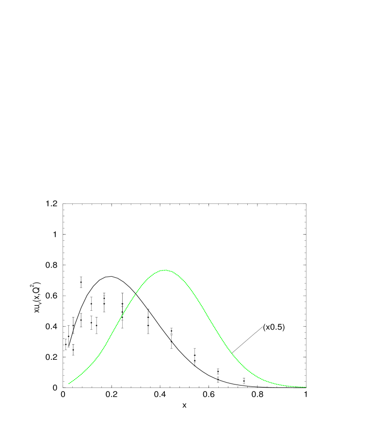
FIG. 1.: The calculated $xu_{v}(x,Q^{2})$ at $Q^{2}={\mu}^{2}=0.1GeV^{2}$ (dotted line) and QCD evolved result at $Q_{0}^{2}=15GeV^{2}$ (solid line) compared with the data taken from T.Sloan et al in Ref.[2]

FIG. 2.: The QCD evolved result for $xd_{v}(x,Q^{2})$ at $Q_{0}^{2}=15GeV^{2}$ (solid line) is given in comparison with the experimental data taken from T.Sloan et al in Ref.[2]

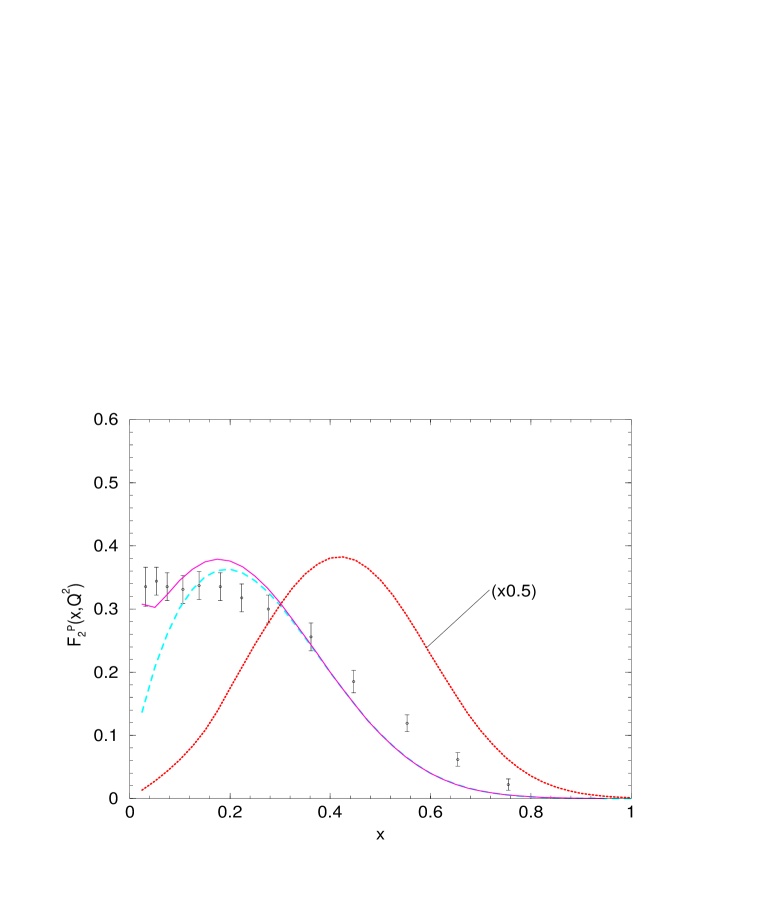
FIG. 3.: The calculated $[F_{2}^{p}(x,Q^{2})]_{val}$ at $Q^{2}={\mu}^{2}=0.1GeV^{2}$ (dotted line) and its QCD evolved result at $Q_{0}^{2}=15GeV^{2}$ (dashed line). $F_{2}^{P}(x,Q^{2})$(valence+asymmetric sea: solid line) in comparison with experimental data taken from R.G.Roberts.et al in Ref.[1].

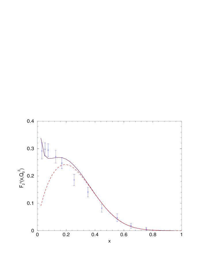
FIG. 4.: The QCD evolved result for $[F_{2}^{n}(x,Q^{2})]_{val}$ at $Q_{0}^{2}=15GeV^{2}$ (dashed line) and $F_{2}^{n}(x,Q^{2})$ (valence+asymmetric sea: solid line) in comparison with data from R.G.Roberts.et al in Ref [1].

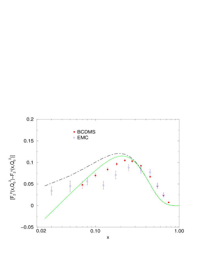
FIG. 5.: The QCD evolved result for $[F_{2}^{p}(x,Q_{0}^{2})-F_{2}^{n}(x,Q_{0}^{2})]$ (dot-dashedline-valence only; solid line- valence+asymmetric sea) at $Q_{0}^{2}=15GeV^{2}$ compared with the data.(data is over the $Q^{2}$-range of the experiments as per Ref.[2])

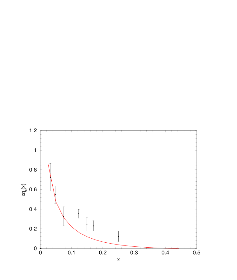
FIG. 6.: The dynamically generated $xq_{s}(x,Q^{2})$(solid line) at $Q_{0}^{2}=15GeV^{2}$, compared with the data from T.Sloan et al in Ref [2].

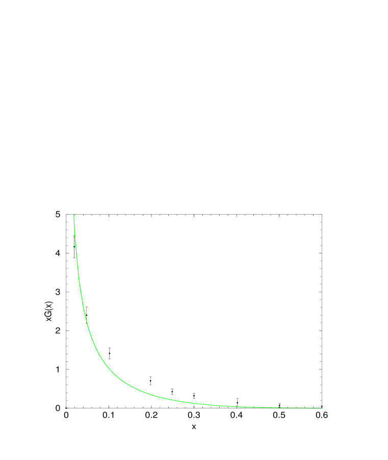
FIG. 7.: The dynamically generated $xG(x,Q^{2})$(solid line) at $Q_{0}^{2}=15GeV^{2}$, compared with the data from T.Sloan et al in Ref [2].

REFERENCES

[1] R. G. Roberts and M. R. Whalley, J. Phys.
, D1 (1991)
S. R. Mishra, F. Sciulli, Ann. Rev. Nucl.
Part. Sci. , 259 (1989) and the references therein.
J. F. Owens, W. K. Tung, Ann. Rev. Nucl. Part. Sci.
, 291 (1992),
A. Milsztajn,A.Staude,K.M.Teichcrt,M.Virchaux,R.Ross., Z. Phys.
, 527 (1991) and the references therein.
P.Amaudruz,M.Arneodo et al.Phys.Rev.Lett. 66,
2712 (1991).
[2] T. Sloan, G. Smadja, R. Voss, Phys. Rep. ,
45 (1988)
J.J.Aubert,G.Bassompierre et al, Nucl.Phys.,740 (1987)
New Muon Collaboration,D.Allasia et al.Report No.CERN-PPE/90-103,1990
BCDMS collaboration;A.C.Benvenuti et al; Phy.Lett.,599(1990)
[3] G. Altarelli, G. Parisi; Nucl. Phys. ,
298 (1977),
Yu.L.Dokshitzer,Zh.Eksp.Fiz.,1216(1977)[Sov.Phys.,
641(1977)];
V.N.Gribov and L.N.Lipatov,Yad. Fiz ,78(1972)[Sov.J.Nucl.Phys
,438(1972)]
[4] M. Göckler,R.Horsley et al.J.Phys ,703(1996)
[5] R.L.Jaffe; Phys.Rev.,1953 (1975);
[6] C. J. Benesh and G. A. Miller, Phys. Rev. ,
1344 (1987);
C. J. Benesh and G. A. Miller,ibid ,
48 (1988)
[7] X. M. Wang, X. Song, P. C. Yin,
Hadron Journal, ,
985 (1983);
X. M. Wang, Phys. Lett. , 413 (1984)
[21] G.Parisi and R.petronzio; Phys. Lett.
, 331 (1976)
V.A.Novikov,M.A.Shifman,A.I.Vainstein and V.I.Zakharov; JETP Lett
, 341 (1976); Ann.Phys. , 276 (1977)
M.Gluck and E.Reya; Nucl.Phys. , 76 (1977)
[22] M.Gluck,R.M.Godbole and E.Reya; Z.Phys , 667 (1989)
[23] M.R.Pennington and G.G.Ross; Phys.Lett.
, 371 (1979)
A.J.Buras; Rev.Mod.Phy. 199 (1980)
Richard D.Field:in ApplicationofPerturbative-QCD
(Addison-Wesley, New York, 1989), p.148.
[24] Callen Gross relation is satisfied in the model
here, since it can be shown that is
finite in the Bjorken limit as ;
[25] M.Arneodo,A.Arvidson et al.Phys.Rev.,R1 (1994)
P.Amadruz,M.Arneodo et al. Phys.Rev.Lett.,2712 (1991)
[26] NA51 Collaboration; A.Baldit,C.Barrire
et al.Phy.Lett ,244,(1994)
Fermilab /NuSea Collaboration;
E.A.Hawker,T.C.Awes et al. Phy.Rev.Lett.,3715 (1998)
CCFR Collaboration; A.O.Bazarko,C.G.Arriyo et al.Z.Phys.
,189(1995)