A systematic study of QCD coupling constant from
deep inelastic measurements

V.G. Krivokhijine

Laboratory of Particle Physics, Joint Institute for Nuclear Research,
141980 Dubna, Russia

and

A.V. Kotikov

Bogoliubov Laboratory of Theoretical Physics, Joint Institute for Nuclear Research,
141980 Dubna, Russia

Abstract

We reanalyze deep inelastic scattering data of BCDMS Collaboration by including proper cuts of ranges with large systematic errors. We perform also the fits of high statistic deep inelastic scattering data of BCDMS, SLAC, NM and BFP Collaborations taking the data separately and in combined way and find good agreement between these analyses. We extract the values of both the QCD coupling constant $\alpha_{s}(M^{2}_{Z})$ up to NLO level and of the power corrections to the structure function $F_{2}$. The fits of the combined data for the nonsinglet part of the structure function $F_{2}$ predict the coupling constant value $\alpha_{s}(M^{2}_{Z})=0.1174\pm 0.0007$ (stat) $\pm 0.0019$ (syst) $\pm 0.0010$ (normalization) (or QCD parameter $\Lambda^{(5)}_{\overline{MS}}=(204\pm 25~{}\mbox{(total exper.err.)})MeV$). The fits of the combined data for both: the nonsinglet part and the singlet one, lead to the values $\alpha_{s}(M^{2}_{Z})=0.1177\pm 0.0007$ (stat) $\pm 0.0021$ (syst) $\pm 0.0009$ (normalization) (or QCD parameter $\Lambda^{(5)}_{\overline{MS}}=(208\pm 27~{}\mbox{(total exper.err.)})MeV$). Both above values are in very good agreement with each other. We estimate theoretical uncertainties for $\alpha_{s}(M^{2}_{Z})$ as $+0.0047$ and $-0.0057$ from fits of the combine data, when complete singlet and nonsinglet $Q^{2}$ evolution is taken into account.

$PACS:~{}~{}12.38~{}Aw,\,Bx,\,Qk$

Keywords: Deep inelastic scattering; Structure functions; QCD coupling constant; $1/Q^{2}$ power corrections.

1 Introduction

The deep inelastic scattering (DIS) leptons on hadrons is the basical process to study the values of the parton distribution functions which are universal (after choosing of factorization and renormalization schemes) and can be used in other processes. The accuracy of the present data for deep inelastic structure functions (SF) reached the level at which the $Q^{2}$-dependence of logarithmic QCD-motivated and power-like ones may be studied separately (for a review, see the recent papers [1, 2] and references therein).

In the present article we analyze at the next-to-leading (NLO) order of perturbative QCD the most known DIS SF $F_{2}(x,Q^{2})$ taking into account SLAC, NMC, BCDMS and BFP experimental data [4]-[10]. We stress the power-like effects, so-called twist-4 (i.e. $\sim 1/Q^{2}$) contributions. To our purposes we represent the SF $F_{2}(x,Q^{2})$ as the contribution of the leading twist part $F_{2}^{pQCD}(x,Q^{2})$ described by perturbative QCD and the nonperturbative part (twist-four terms $\sim 1/Q^{2}$):

$$F_{2}(x,Q^{2})\equiv F_{2}^{full}(x,Q^{2})=F_{2}^{pQCD}(x,Q^{2})+\frac{\tilde{h}_{4}(x)}{Q^{2}}$$ (1)

The SF $F_{2}^{pQCD}(x,Q^{2})$ obeys the (leading twist) perturbative QCD dynamics including the target mass corrections (TMC) (and coincides with $F_{2}^{tw2}(x,Q^{2})$ when the target mass corrections are withdrawn).

The Eq.(1) allows us to separate pure kinematical power corrections, i.e. TMC, so that the function $\tilde{h}_{4}(x)$ corresponds to “dynamical” contribution of the twist-four operators. The parameterization (1) implies that the anomalous dimensions of the twist-four operators are equal to zero, that is not correct in principle. Moreover, there are estimations of these anomalous dimensions (see [11]). Meanwhile, in view of limited precision of the data, the approximation (1) and one in the footnote 2 give rather good predictions (see discussions in [12, 13]).

Contrary to standard fits (see, for example, [14, 15]) when the direct numerical calculations based on Dokshitzer-Gribov-Lipatov-Altarelli-Parisi (DGLAP) equation [16] are used to evaluate structure functions, we use the exact solution of DGLAP equation for the Mellin moments $M_{n}^{tw2}(Q^{2})$ of SF $F_{2}^{tw2}(x,Q^{2})$:

$$M_{n}^{k}(Q^{2})=\int_{0}^{1}x^{n-2}\,F_{2}^{k}(x,Q^{2})\,dx~{}~{}~{}~{}~{}~{}~{}(\mbox{hereafter }k=full,pQCD,tw2,...)$$ (2)

and the subsequent reproduction of $F_{2}^{full}(x,Q^{2})$, $F_{2}^{pQCD}(x,Q^{2})$ and/or $F_{2}^{tw2}(x,Q^{2})$ at every needed $Q^{2}$-value with help of the Jacobi Polynomial expansion method [17]-[19] (see similar analyses at the NLO level [18]-[21] and at the NNLO level and above [22]-[27]).

The method of the Jacobi polynomial expansion was developed in [17, 18] and described in details in Refs.[19]. Here we consider only some basical definitions in Section 3.

The paper has the following structure: in Section 2 we present basic formulae, which are needed in our analyses: we consider different types of $Q^{2}$-dependence of SF moments, effects of nuclear corrections and heavy quark thresholds, the structure of normalization of parton densities in singlet and nonsinglet channels. In Section 3 we introduce the basic elements of our fits. Sections 4 and 5 contain conditions and results of several types of fits with the nonsinglet and singlet evolutions for different sets of data. In Section 6 we study the dependence of the results on choice of factorization and renormalization scales. In Section 7 we summarize the basic observations following from the fits and discuss possible future extensions of the analyses.

2 $Q^{2}$ dependence of SF and their moments

In this section we analyze Eq.(1) in detail, considering separately different types of $Q^{2}$-dependence of structure function $F_{2}$.

2.1 The leading-twist $Q^{2}$ dependence

To study the $Q^{2}$-dependence of the SF $F_{2}^{tw2}(x,Q^{2})=F_{2}^{NS}(x,Q^{2})+F_{2}^{S}(x,Q^{2})$, which splits explicitly into the nonsinglet (NS) part and the singlet (S) one, it is very useful to introduce parton distribution functions (PDF): gluon one $f_{G}(x,Q^{2})$ and singlet and nonsinglet quarks ones $f_{S}(x,Q^{2})$ and $f_{NS}(x,Q^{2})$.

The moments $M_{n}^{NS}(Q^{2})$ and $M_{n}^{S}(Q^{2})$ of NS and S parts of SF $F_{2}$ (see Eq.(2) for definition) are connected with the corresponding moments of PDF $f_{i}(x,Q^{2})$ (hereafter $i=NS,S,G$)

$$f_{i}(n,Q^{2})=\int_{0}^{1}x^{n-2}f_{i}(n,Q^{2})dx$$

in the following way (see [28], for example)

$$M_{n}^{NS}(Q^{2}) = K_{NS}(f)\cdot C_{NS}^{tw2}(n,\overline{a}_{s}(Q^{2}))\cdot f_{NS}(n,Q^{2})$$

$$M_{n}^{S}(Q^{2}) = K_{S}(f)\cdot\biggl{[}C_{S}^{tw2}(n,\overline{a}_{s}(Q^{2}))\cdot f_{S}(n,Q^{2})+C_{G}^{tw2}(n,\overline{a}_{s}(Q^{2}))\cdot f_{G}(n,Q^{2})\biggr{]},$$

where

$$\overline{a}_{s}(Q^{2})~{}=~{}\frac{\alpha_{s}(Q^{2})}{4\pi}$$ (4)

and $C_{i}^{tw2}(n,\overline{a}_{s}(Q^{2}))$ are so-called Wilson coefficient functions. We have introduced here also the coefficients

$$K_{S}(f)~{}=~{}\sum^{f}_{m=1}e^{2}_{m}/f,~{}~{}~{}~{}~{}~{}K_{NS}(f)~{}=~{}e^{2}_{u}-K_{S}(f),$$ (5)

which come from definition of SF $F_{2}$ (see, for example, [28]). Here $f$ is the number of active quarks and $e^{2}_{m}$ is charge square of the active quark of $m$ flavor.

2.1.1   The dependence of $\overline{a}_{s}(Q^{2})$ is given by the renormalization group equation, which in the NLO QCD approximation reads:

$$\frac{1}{\overline{a}_{s}(Q^{2})}-\frac{1}{\overline{a}_{s}(M_{Z}^{2})}+\frac{\beta_{1}}{\beta_{0}}\ln{\left[\frac{\overline{a}_{s}(Q^{2})}{\overline{a}_{s}(M_{Z}^{2})}\frac{\left(\beta_{0}+\beta_{1}\overline{a}_{s}(M_{Z}^{2})\right)}{\left(\beta_{0}+\beta_{1}\overline{a}_{s}(Q^{2})\right)}\right]}=\beta_{0}\ln{\left(\frac{Q^{2}}{M_{Z}^{2}}\right)},$$ (6)

where $\overline{a}_{s}(M_{Z}^{2})$ is served as a normalization. Here and below we use $\beta_{0}$ and $\beta_{1}$ for the first and the second terms with respect to $\overline{a}_{s}$ of QCD $\beta$-function:

$$\beta(\overline{a}_{s})~{}=~{}-\beta_{0}\overline{a}_{s}^{2}-\beta_{1}\overline{a}_{s}^{3}~{}+~{}...~{}~{}.$$

The equation (6) allows us to eliminate the QCD parameter $\Lambda_{QCD}$ from our analysis. However, sometimes we will present it in our discussions, essentially to compare it with the results of old fits. The coupling constant $\overline{a}_{s}(Q^{2})$ is expressed through $\Lambda_{QCD}$ (in $\overline{\rm MS}$ scheme, where $\Lambda_{QCD}=\Lambda_{\overline{\rm MS}}$) as

$$\frac{1}{\overline{a}_{s}(Q^{2})}+\frac{\beta_{1}}{\beta_{0}}\ln{\left[\frac{\beta_{0}^{2}\overline{a}_{s}(Q^{2})}{\left(\beta_{0}+\beta_{1}\overline{a}_{s}(Q^{2})\right)}\right]}=\beta_{0}\ln{\left(\frac{Q^{2}}{\Lambda^{2}_{\overline{\rm MS}}}\right)},$$ (7)

The relation between the normalization $\overline{a}_{s}(M_{Z}^{2})$ and the QCD parameter $\Lambda_{QCD}$ can be obtained from Eq.(7) with the replacement $Q^{2}\to M_{Z}^{2}$.

We would like to note that the approximations of Eq.(7), based on the expansion of inverse powers of $\ln{\left(Q^{2}/\Lambda^{2}_{\overline{\rm MS}}\right)}$ are very popular. The accuracy of these expansions for evolution of $\overline{a}_{s}$ from $O$(GeV²) to $M_{Z}^{2}$ may be as large as $0.001$ [13], which is comparable with the experimental uncertainties of the $\alpha_{s}(M_{Z}^{2})$ value extracted from the data (see our analyses in Sections 4 and 5).

Note also that sometimes (see, for example, [22]) the equation

$$\frac{1}{\overline{a}_{s}(Q^{2})}+\frac{\beta_{1}}{\beta_{0}}\ln{\left(\beta_{0}\overline{a}_{s}(Q^{2})\right)}=\beta_{0}\ln{\left(\frac{Q^{2}}{\Lambda^{2}_{\overline{\rm MS}}}\right)},$$ (8)

is used in analyses. This equation can be obtained from the basic equation

$$\ln{\left(\frac{Q^{2}}{\Lambda^{2}_{\overline{\rm MS}}}\right)}~{}=~{}\int^{\overline{a}_{s}(Q^{2})}\frac{db}{\beta(b)},$$ (9)

by expansion of inverse QCD $\beta$-function in r.h.s. of (9) $1/\beta(\overline{a}_{s})$ in powers of $\overline{a}_{s}$. The difference between Eqs.(8) and (7) may be as large as $0.001$ at $O$(GeV²) range. In order to escape the above uncertainties we use in the analyses the exact numerical solution (with accuracy about $10^{-5}$) of Eq.(6) instead. For recalculation of the QCD parameter $\Lambda_{\overline{\rm MS}}$ from $\Lambda^{(f)}_{\overline{\rm MS}}$ to $\Lambda^{(f\pm 1)}_{\overline{\rm MS}}$ (i.e. from $\Lambda_{\overline{\rm MS}}$ at $f$ active quark flavors to $\Lambda_{\overline{\rm MS}}$ at $f\pm 1$ active quark flavors), because $\beta_{0}$ and $\beta_{1}$ are $f$-dependent functions, we use formulae at NLO approximation from Ref. [29] (see discussions in the subsection 2.4).

2.1.2   The coefficient functions $C_{i}^{tw2}(n,\overline{a}_{s}(Q^{2}))$ ($i=NS,S,G$) have the following form

$$C_{i}^{tw2}(n,\overline{a}_{s}(Q^{2}))=1-\delta^{G}_{i}+\overline{a}_{s}\cdot B_{i}(n)+O(\overline{a}_{s}^{2})~{}~{}~{}~{}(\delta^{m}_{i}~{}\mbox{is Kronecker symbol}),$$ (10)

where the NLO coefficients $B_{i}(n)$ are exactly known (see, for example, [28]).

The $Q^{2}$-evolution of the moments $f_{i}(n,Q^{2})$ is given by the well known perturbative QCD [28, 30] formulae:

$$\frac{f_{NS}(n,Q^{2})}{f_{NS}(n,Q_{0}^{2})} = \bigg{[}\frac{\overline{a}_{s}(Q_{0}^{2})}{\overline{a}_{s}(Q^{2})}\bigg{]}^{\gamma_{NS}^{(0)}(n)/2\beta_{0}}\cdot H^{NS}(n,Q^{2},Q_{0}^{2})~{}~{}~{},$$

$$f_{j}(n,Q^{2}) = f_{j}^{+}(n,Q^{2})+f_{j}^{-}(n,Q^{2})~{}~{}~{}~{}~{}(j=S,G)$$ (11)

$$\frac{f_{j}^{\pm}(n,Q^{2})}{f_{j}^{\pm}(n,Q_{0}^{2})} = \bigg{[}\frac{\overline{a}_{s}(Q_{0}^{2})}{\overline{a}_{s}(Q^{2})}\bigg{]}^{\gamma_{\pm}^{(0)}(n)/2\beta_{0}}\cdot H_{j}^{\pm}(n,Q^{2},Q_{0}^{2})~{}~{}~{},$$

where

$$f_{j}^{\pm}(n,Q^{2}) = \varepsilon_{jl}^{\pm}(n)f_{l}(n,Q^{2}),~{}~{}~{}~{}~{}(j,l=S,G)$$ (12)

$$\gamma_{\pm}^{(0)}(n) = \frac{1}{2}\Biggl{[}\Bigl{(}\gamma_{GG}^{(0)}(n)+\gamma_{SS}^{(0)}(n)\Bigr{)}\pm\sqrt{\Bigl{(}\gamma_{SS}^{(0)}(n)-\gamma_{GG}^{(0)}(n)\Bigr{)}+4\gamma_{GS}^{(0)}(n)\gamma_{SG}^{(0)}}\Biggr{]}$$

$$\varepsilon_{qq}^{\pm}(n) = \varepsilon_{gg}^{\mp}(n)=\frac{1}{2}\biggl{(}1+\frac{\gamma_{SS}^{(0)}(n)-\gamma_{GG}^{(0)}(n)}{\gamma_{\pm}^{(0)}(n)-\gamma_{\mp}^{(0)}(n)}\biggr{)},~{}~{}\varepsilon_{jl}^{\pm}(n)=\frac{\gamma_{jl}^{(0)}(n)}{\gamma_{\pm}^{(0)}(n)-\gamma_{\mp}^{(0)}(n)}~{}~{}~{}(j\neq l)$$

The functions $H^{NS}(n,Q^{2},Q^{2}_{0})$ and $H_{j}^{\pm}(n,Q^{2},Q^{2}_{0})$ are nonzero above the leading order (LO) approximation and may be represented as

$$H^{NS}(n,Q^{2},Q^{2}_{0}) = 1+\Bigl{(}\overline{a}_{s}(Q^{2})-\overline{a}_{s}(Q^{2}_{0})\Bigr{)}Z_{NS}(n)+O\Bigl{(}\overline{a}_{s}^{2}(Q^{2})\Bigr{)}$$

$$H_{j}^{\pm}(n,Q^{2},Q^{2}_{0}) = 1+\Bigl{(}\overline{a}_{s}(Q^{2})-\overline{a}_{s}(Q^{2}_{0})\Bigr{)}Z_{\pm\pm}(n)$$

$$+ \Biggl{(}\overline{a}_{s}(Q^{2}_{0})\bigg{[}\frac{\overline{a}_{s}(Q_{0}^{2})}{\overline{a}_{s}(Q^{2})}\bigg{]}^{\biggl{(}\gamma_{\mp}^{(0)}(n)-\gamma_{\pm}^{(0)}(n)\biggr{)}/2\beta_{0}}-\overline{a}_{s}(Q^{2})\Biggr{)}Z^{j}_{\pm\mp}(n)+O\Bigl{(}\overline{a}_{s}^{2}(Q^{2})\Bigr{)},$$

where

$$Z_{NS}(n) = \frac{1}{2\beta_{0}}\biggl{(}\gamma_{NS}^{(1)}(n)-\gamma_{NS}^{(0)}(n)\cdot\frac{\beta_{1}}{\beta_{0}}\biggr{)}$$ (14)

$$Z_{\pm\pm}(n) = \frac{1}{2\beta_{0}}\biggl{(}\gamma_{\pm\pm}^{(1)}(n)-\gamma_{\pm}^{(0)}(n)\cdot\frac{\beta_{1}}{\beta_{0}}\biggr{)}$$ (15)

$$Z^{S}_{\pm\mp}(n) = \frac{\gamma_{\pm\mp}^{(1)}(n)}{2\beta_{0}+\gamma_{\pm}^{(0)}(n)-\gamma_{\mp}^{(0)}(n)},~{}~{}~{}Z^{G}_{\pm\mp}(n)=Z^{S}_{\pm\mp}(n)\cdot\frac{\varepsilon^{\mp}_{GG}}{\varepsilon^{\mp}_{SS}}$$ (16)

and

$$\gamma_{\pm\pm}^{(1)}(n) = \sum_{j,l=S,G}\varepsilon^{\pm}_{lj}\gamma^{(1)}_{jl}$$ (17)

$$\gamma_{\pm\mp}^{(1)}(n) = \sum_{j=S,G}\varepsilon^{\pm}_{jG}\gamma^{(1)}_{Gj}-\varepsilon^{\mp}_{SS}\gamma^{(1)}_{SS}+\Bigl{(}\varepsilon^{\pm}_{GS}-\varepsilon^{\pm}_{GG}/\varepsilon^{\pm}_{SG}\Bigr{)}\gamma^{(1)}_{GG}$$

As usually, here we use $\gamma_{NS}^{(0)}(n)$, $\gamma_{jl}^{(0)}(n)$ $(j,l=S,G)$ and $\gamma_{NS}^{(1)}(n)$, $\gamma_{jl}^{(1)}(n)$ as the first and the second terms with respect to $\overline{a}_{s}$ of anomalous dimensions $\gamma_{NS}(n,\overline{a}_{s})$ and $\gamma_{jl}(n,\overline{a}_{s})$ (see, for example, [35]).

2.1.3   In this subsection, we would like to discuss a possible dependence of our results on the factorization scale $\mu_{F}$ and the renormalization scale $\mu_{R}$, which appear (see, for example, [14, 36]) because perturbative series are truncated. These scales $\mu^{2}_{F}=k_{F}Q^{2}$ and $\mu^{2}_{R}=k_{R}\mu^{2}_{F}=k_{R}k_{F}Q^{2}$ can be added to the r.h.s. of the equations (LABEL:3.a) and (11), respectively.

Then, the equations (LABEL:3.a) are replaced by

$$M_{n}^{NS}(Q^{2}) = K_{NS}(f)\cdot\hat{C}_{NS}^{tw2}(n,\overline{a}_{s}(k_{F}Q^{2}))\cdot f_{NS}(n,k_{F}Q^{2})$$

$$M_{n}^{S}(Q^{2}) = K_{S}(f)\cdot\biggl{[}\hat{C}_{S}^{tw2}(n,\overline{a}_{s}(k_{F}Q^{2}))\cdot f_{S}(n,k_{F}Q^{2})+\hat{C}_{G}^{tw2}(n,\overline{a}_{s}(k_{F}Q^{2}))\cdot f_{G}(n,k_{F}Q^{2})\biggr{]}~{}.$$

The equations (11) are replaced correspondingly by

$$\frac{f_{NS}(n,k_{F}Q^{2})}{f_{NS}(n,k_{F}Q_{0}^{2})} = \bigg{[}\frac{\overline{a}_{s}(k_{F}k_{R}Q_{0}^{2})}{\overline{a}_{s}(k_{F}k_{R}Q^{2})}\bigg{]}^{\gamma_{NS}^{(0)}(n)/2\beta_{0}}\cdot\hat{H}^{NS}(n,k_{F}k_{R}Q^{2},k_{F}k_{R}Q_{0}^{2})~{}~{}~{},$$

$$\frac{f_{j}^{\pm}(n,k_{F}Q^{2})}{f_{j}^{\pm}(n,k_{F}Q_{0}^{2})} = \bigg{[}\frac{\overline{a}_{s}(k_{F}k_{R}Q_{0}^{2})}{\overline{a}_{s}(k_{F}k_{R}Q^{2})}\bigg{]}^{\gamma_{\pm}^{(0)}(n)/2\beta_{0}}\cdot\hat{H}_{j}^{\pm}(n,k_{F}k_{R}Q^{2},k_{F}k_{R}Q_{0}^{2})~{}.$$

The coefficients $\hat{C}_{NS}$, $\hat{C}_{S}$, $\hat{C}_{G}$, $\hat{H}^{NS}$ and $\hat{H}_{j}^{\pm}$ can be obtained from the ones $C_{NS}$, $C_{S}$, $C_{G}$, $H^{NS}$ and $H_{j}^{\pm}$ by modification in the r.h.s. of equations (10), (14) and (15) as follows:

in Eq. (10)

$$\overline{a}_{s}(Q^{2}) \to \overline{a}_{s}(k_{F}Q^{2})$$ (20)

$$B_{NS}(n) \to B_{NS}(n)+\frac{1}{2}\gamma_{NS}^{(0)}(n)\ln{k_{F}}$$

$$B_{j}(n) \to B_{j}(n)+\frac{1}{2}\gamma_{jS}^{(0)}(n)\ln{k_{F}}~{}~{}~{}~{}~{}~{}(j=S,G)$$ (21)

in Eqs. (14) and (15)

$$\overline{a}_{s}(Q^{2}) \to \overline{a}_{s}(k_{F}k_{R}Q^{2})$$ (22)

$$Z_{NS}(n) \to Z_{NS}(n)+\frac{1}{2}\gamma_{NS}^{(0)}(n)\ln{k_{R}}$$

$$Z_{\pm\pm}(n) \to Z_{\pm\pm}(n)+\frac{1}{2}\gamma^{(0)}_{\pm}(n)\ln{k_{R}}$$ (23)

The Eqs. (21) can be obtained easily using, for example, the results of [37]. The Eqs. (23) can be found from the expansion of the coupling constant $\overline{a}_{s}(k_{F}k_{R}Q^{2})$ around the one $\overline{a}_{s}(Q^{2})$ in the r.h.s. of the exact solution of DGLAP equations (see Eqs.(LABEL:3l) and (2.1)).

The changes (21) and (23) of the results for $Q^{2}$-dependence under variation of $k_{F}$ and $k_{R}$ (usually from $1/2$ to $2$) give an estimation of the errors due to renormalization and factorization scale uncertainties. Evidently that, by definition, these uncertainties are connected with the impact of unaccounted terms of the perturbative series and can represent theoretical uncertainties in values of fitted variables. Indeed, an incorporation of NNLO corrections to the analysis strongly suppress these uncertainties (see [39, 40]).

We study exactly the $\mu_{F}$ and $\mu_{R}$ dependences here for fitted values of coupling constant. The results of the study are given in the Section 6.

As one can see in Eqs. (20) and (22), the coupling constant $\overline{a}_{s}$ has different arguments in the NLO corrections of coefficient functions $\hat{C}_{NS}$ and $\hat{C}_{j}$ ($j=S,G$) and in the NLO corrections $\hat{H}^{NS}$ and $\hat{H}_{j}^{\pm}$ of the $Q^{2}$-evolution of parton distributions. We would like to note that the difference between the corresponding coupling constants $\overline{a}_{s}(k_{F}Q^{2})$ and $\overline{a}_{s}(k_{F}k_{R}Q^{2})$ is proportional to $\overline{a}_{s}^{2}$ and, thus, mathematically negligible in our NLO approximation.
Then, we can use the replacement (22) in coefficient functions too, as it has been done in previous studies [38, 39, 40, 27]. We note that the replacement $\overline{a}_{s}(k_{F}Q^{2})\to\overline{a}_{s}(k_{F}k_{R}Q^{2})$ in Eq. (20) increases slightly the factorization scheme dependence of the results for coupling constant (see analyses based on nonsinglet evolution and discussions in Section 6).

2.2 Normalization of parton distributions

The moments $f_{i}(n,Q^{2})$ at some $Q^{2}_{0}$ is theoretical input of our analysis which is fixed as follows.

For fits of data at $x\geq 0.25$ we can work only with the nonsinglet parton density and use directly its normalization $\tilde{f}_{NS}(x,Q_{0}^{2})$ (see, for example, [22]-[26]):

$$f_{NS}(n,Q_{0}^{2}) = \int_{0}^{1}dxx^{n-2}\tilde{f}_{NS}(x,Q_{0}^{2}),$$

$$\tilde{f}_{NS}(x,Q_{0}^{2}) = A_{NS}(Q_{0}^{2})(1-x)^{b_{NS}(Q_{0}^{2})}(1+d_{NS}(Q_{0}^{2})x)$$ (24)

where $A_{NS}(Q_{0}^{2})$, $b_{NS}(Q_{0}^{2})$ and $d_{NS}(Q_{0}^{2})$ are some coefficients .

At the analyses at arbitrary values of $x$ we should introduce the normalizations for densities of individual quarks $(q=u,d,s,...)$ and antiquarks $(\overline{q}=\overline{u},\overline{d},\overline{s},...)$ $\tilde{f}_{q}(x,Q_{0}^{2})$ and $\tilde{f}_{\overline{q}}(x,Q_{0}^{2})$ having the moments:

$$f_{i}(n,Q_{0}^{2})~{}=~{}\int_{0}^{1}dxx^{n-2}\tilde{f}_{i}(x,Q_{0}^{2}),$$ (25)

The distributions of $u$ and $d$ quarks $\tilde{f}_{u}(x,Q_{0}^{2})\equiv u(x,Q_{0}^{2})$ and $\tilde{f}_{d}(x,Q_{0}^{2})\equiv d(x,Q_{0}^{2})$ are split in two components: the valent one $u_{v}(x,Q_{0}^{2})$ and $d_{v}(x,Q_{0}^{2})$ and the sea one $u_{v}(x,Q_{0}^{2})$ and $d_{v}(x,Q_{0}^{2})$. For other quark distributions and antiquark densities we keep only sea parts. Moreover, following [28, 41] we suppose equality of all sea parts and mark their sum as $S(x,Q_{0}^{2})$.

We use the following parameterizations for densities $u_{v}(x,Q_{0}^{2})$, $u_{v}(x,Q_{0}^{2})$, $S(x,Q_{0}^{2})$ $\tilde{f}_{G}(x,Q_{0}^{2})$:

$$u_{v}(x,Q_{0}^{2}) = \frac{2}{B(a_{u}(Q_{0}^{2}),b_{u}(Q_{0}^{2})+1)}\,x^{a_{u}(Q_{0}^{2})}(1-x)^{b_{u}(Q_{0}^{2})},$$

$$d_{v}(x,Q_{0}^{2}) = \frac{1}{B(a_{d}(Q_{0}^{2}),b_{d}(Q_{0}^{2})+1)}\,x^{a_{d}(Q_{0}^{2})}(1-x)^{b_{d}(Q_{0}^{2})},$$ (26)

$$S(x,Q_{0}^{2}) = C_{S}(Q_{0}^{2})x^{a_{S}(Q^{2}_{0})}(1-x)^{b_{S}(Q_{0}^{2})},~{}~{}~{}~{}~{}~{}$$

$$\tilde{f}_{G}(x,Q_{0}^{2}) = C_{G}(Q_{0}^{2})x^{a_{G}(Q^{2}_{0})}(1-x)^{b_{G}(Q_{0}^{2})},$$ (27)

where $B(a,b)$ is the Euler beta-function. The parameterizations (26) have been chosen to satisfy (at the normalization point $Q^{2}_{0}$) the known rule:

$$\int_{0}^{1}dxV(x,Q^{2})=3,$$

where $V(x,Q^{2})=u_{v}(x,Q^{2})+d_{v}(x,Q^{2})$ is the distribution of valent quarks.

We note that the nonsinglet and singlet parts of quark distributions $\tilde{f}_{NS}(x,Q_{0}^{2})$ and $\tilde{f}_{S}(x,Q_{0}^{2})$ can be represented as combination of quark ones

$$\tilde{f}_{S}(x,Q_{0}^{2}) \equiv \sum_{q}^{f}\tilde{f}_{q}(x,Q_{0}^{2})~{}=~{}V(x,Q_{0}^{2})+S(x,Q_{0}^{2})$$ (28)

$$\tilde{f}_{NS}(x,Q_{0}^{2}) = u_{v}(x,Q_{0}^{2})-d_{v}(x,Q_{0}^{2}),$$ (29)

where the r.h.s. of Eq.(29) is correct only in the framework of our supposition about equality of antiquarks distributions and sea components of quark ones.

In principle, following the PDF models used in [15, 12] and above Eq.(24) one can add in Eq.(27) terms proportional to $\sqrt{x}$ and $x$. However, the terms $\sim\sqrt{x}$ are important only in the region of rather small $x$ (see discussion in [12]). The terms $\sim x$ lead only to replacement of $C_{i}$, $a_{i}$ and $b_{i}$ values (see, for example, [42]). Thus, we neglect these terms in our analysis.

In the most our fits we do not take into account also the terms $\sim x^{a_{G}(Q^{2}_{0})}$ and $\sim x^{a_{S}(Q^{2}_{0})}$ into gluon and sea quark distributions, because we do not consider experimental data at small values of Bjorken variable $x$ . We hope to include H1 and ZEUS data [43, 44] in our future investigations [45] and then to study $Q^{2}$-dependence of the coefficients $a_{G}(Q^{2})$ and $a_{S}(Q^{2})$, which could be very nontrivial (see, for example, Refs. [46, 48, 43, 32] and references therein).

We impose also the condition for full momentum conservation in the form:

$$1~{}=~{}P_{G}(Q^{2})+P_{q}(Q^{2}),$$ (30)

where

$$P_{G}(Q^{2}) = \int_{0}^{1}dx\tilde{f}_{G}(x,Q^{2}),$$

$$P_{q}(Q^{2}) = \int_{0}^{1}dx\biggl{(}\tilde{f}_{NS}(x,Q^{2})+\tilde{f}_{S}(x,Q^{2})\biggr{)},$$ (31)

The coefficients $C_{i}(Q_{0}^{2})$, $a_{i}(Q_{0}^{2})$, $b_{i}(Q_{0}^{2})$, $c_{i}(Q_{0}^{2})$ and $d_{i}(Q_{0}^{2})$ should be found together with $h_{4}(x)$ (see subsection 2.6) and the normalization $\alpha_{s}(M^{2}_{Z})$ of QCD coupling constant (or QCD parameter $\Lambda$) by the fits of experimental data.

2.3 Target mass corrections

The target mass corrections [49, 28] modify the SF $F_{2}^{NS}(x,Q^{2})$ in the following way

$$F_{2}^{pQCD}(x,Q^{2}) = \frac{1}{r^{3}}\frac{x^{2}}{\xi^{2}}F_{2}^{tw2}(\xi,Q^{2})+6\frac{M_{nucl.}^{2}}{Q^{2}}\frac{x^{3}}{r^{6}}\int^{1}_{\xi}\frac{d\xi^{\prime}}{(\xi^{\prime})^{2}}F_{2}^{tw2}(\xi^{\prime},Q^{2})$$ (32)

$$+ 12\frac{M_{nucl.}^{4}}{Q^{4}}\frac{x^{4}}{r^{5}}\int^{1}_{\xi}\int^{1}_{\xi^{\prime}}\frac{d\xi^{\prime\prime}}{(\xi^{\prime\prime})^{2}}F_{2}^{tw2}(\xi^{\prime\prime},Q^{2})$$

where $M_{nucl}$ is the mass of the nucleon, $r=\sqrt{1+x^{2}M_{nucl.}^{2}/Q^{2}}$ and the Nachtmann variable $\xi=2x/(1+r)$.

In our analyses below, we will use all this (32) representation . We would like to keep the full value of kinematic power corrections, given by nonzero nucleon mass. Then, the excess of $1/Q^{2}$ dependence encoded in experimental data will give the magnitude of twist-four corrections, which is most important part of dynamical power corrections.

2.4 Thresholds of heavy quarks

Modern estimates performed in  [51, 52] have revealed a quite significant role of threshold effects in the $\alpha_{s}(Q^{2})$ evolution when the DIS data lie close to threshold points $Q^{2}=M_{f+1}^{2}\sim m_{f+1}^{2}$ (to the position of so-called ”Euclidean–reflected” threshold of heavy particles). The corresponding corrections to the normalization $\alpha_{s}(M^{2}_{Z})$ can reach several percent, i.e. , they are of the order of other uncertainties which should be under control at our analysis.

An appropriate procedure for the inclusion of threshold effects into the $Q^{2}$–dependence of $\alpha_{s}(Q^{2})$ in the framework of the massless $\overline{\rm MS}$ scheme was proposed more than 10 years ago  [53, 54] : transition from the region with a given number of flavors $f$ described by massless $\alpha_{s}(Q^{2};f)$ to the next one with $f+1$ (“transition across the $M_{f+1}$ threshold”) is realized here with the use of the so–called “matching relation” for $\alpha_{s}(Q^{2})$  [54]. The latter may be considered as the continuity condition for $\alpha_{s}(Q^{2})$ on (every) heavy quark mass $m_{f+1}$

$$\alpha_{s}(Q^{2}=M^{2}_{f+1};f) = \alpha_{s}(Q^{2}=M^{2}_{f+1};f+1)~{}~{}~{}~{}~{}~{}~{}~{}\mbox{ and }$$ (33)

$$M_{f+1} = m_{f+1}$$ (34)

that provides an accurate $\alpha_{s}(Q^{2})$–evolution description for $Q^{2}$ values not close to the threshold region (see [55] and references therein).

At the analyses based on nonsinglet evolution, the additional $f$-dependence comes only from the NLO correction of NS anomalous dimensions (see [35]) . In the Section 3 we check numerically the dependence of the results from the matching point. We use two matching points: (34) one and

$$M_{f+1}~{}=~{}2\,m_{f+1}$$ (35)

and demonstrate very little variations of the results (see Section 4 and discussion there).

As we know, for singlet part of evolution no simple recipe exists for exact value of the matching point $M_{f+1}$. From one side, as in the nonsinglet case, there is $Q^{2}$-evolution of the SF moments which leads to above condition (34). But here we have also the generation of heavy quarks (at lowest nontrivial order, in the framework of the photon-gluon fusion process), that gives contributions to gluon part of the singlet coefficient function. The photon-gluon fusion needs the matching point at the value of $Q^{2}$, when $W^{2}=4m_{f+1}^{2}$, i.e.

$$M_{f+1}^{2}\cdot\frac{1-x}{x}+M^{2}_{nucl.}~{}=~{}4m_{f+1}^{2}$$ (36)

At small $x$ values the condition (36) is quite close to the one (34) (for example, at $x=0.2$ $M_{f+1}^{2}~{}=~{}m_{f+1}^{2}-M^{2}_{nucl.}/4$), but at the range of large and intermediate values of $x$, the value of $M_{f+1}$ is essentially large to compare with one of Eq.(34). For example, at $x=0.5$ $M_{f+1}^{2}~{}=~{}4m_{f+1}^{2}-M^{2}_{nucl.}$, that is very close to the matching point (35). At larger $x$ values the value of $M_{f+1}^{2}$ will be close to ones in [38, 39].

We note, that the difference between nonsinglet and singlet $Q^{2}$-dependences comes from contribution of gluon distribution. The contribution is negligible at $x>0.3$ that supports qualitatively the choice (34) as the matching point.

We would like to note also, that at NLO approximation and above, the situation is even more difficult in singlet case, because every subprocess generates itself matching point $M_{f+1}$ to coefficient functions. To estimate a possible effect of a dependence on matching point, we will fit data (in Section 3) with two different matching points: (34) one and (35) one. Surprisingly, at the singlet case, where all functions coming to $Q^{2}$-evolution are $f$-dependent, we do not find a strong $f$-dependence of our results (see Section 5 and discussions there).

2.5 Nuclear effects

Starting with EMC discovery in [57], it is well known about the difference between PDF in free hadrons and ones in hadrons in nuclei. We incorporate the difference in our analyses.

In the nonsinglet case we parameterize the initial PDF in the form (24) for every type of target. We have

$$f^{A}_{NS}(n,Q_{0}^{2})~{}=~{}\int_{0}^{1}dxx^{n-2}\tilde{f}^{A}_{NS}(x,Q_{0}^{2}),$$ (37)

where

$$\tilde{f}^{A}_{NS}(x,Q_{0}^{2})~{}=~{}A^{A}_{NS}(Q_{0}^{2})(1-x)^{b^{A}_{NS}(Q_{0}^{2})}(1+d^{A}_{NS}(Q_{0}^{2})x)$$ (38)

and $A=H,~{}D,~{}C$ and $F$ in the case of $H_{2},~{}D_{2},~{}C^{12}$ and $Fe^{56}$ targets, respectively.

In the singlet case we have many parameters in our fits, which should be fitted very carefully. The representations similar to (38) for gluon and sea quark PDF should complicate our analyses. To overcome the problem, we apply the Eqs. (37) and (38) only to $H_{2}$ and $D_{2}$ cases. For heavier targets we apply simpler representations for $F_{2}^{A}$ structure functions in the form:

$$F^{A}_{2}(x,Q^{2})~{}=~{}F^{D}_{2}(x,Q^{2})\cdot K^{A}_{1}\Bigl{(}1-K^{A}_{2}x+K^{A}_{3}x^{2}\Bigr{)}~{}~{}~{}~{}~{}(A=C^{12},Fe^{56}),$$ (39)

where we use experimental observation (see [60] and references therein) about approximate $Q^{2}$-independence of EMC ration $F^{A}_{2}/F^{D}_{2}$.

2.6 Higher-twist corrections

For $n$-space eq.(1) transforms to

$$M_{n}^{full}(Q^{2})~{}=~{}M_{n}^{pQCD}(Q^{2})+\frac{h_{4}(n)}{Q^{2}},$$ (40)

where $h_{4}(n,Q^{2})$ are the moments of the function $\tilde{h}_{4}(x,Q^{2})$:

$$h_{4}(n)=\int_{0}^{1}x^{n-2}\tilde{h}_{4}(x)dx$$ (41)

The shape $\tilde{h}_{4}(x)$ (or coefficients $h_{4}(n)$) of the twist-four corrections are of primary consideration in our analysis. They can be chosen in the several different forms:

• the twist-four terms (and twist-six ones) are fixed in agreement with the infrared renormalon (IRR) model (see [61, 62, 1, 2] and references therein).

• The twist-four term in the form $h_{4}(x)\sim\frac{d}{dx}lnF_{2}^{NS}(x,Q^{2})\sim 1/(1-x)$ (see [30] and references therein). This behavior matches the fact that higher twist effects are usually important only at higher $x$. The twist-four coefficient function has the form $C_{4}^{der}(n)=(n-1)A_{4}^{der}$.

• The twist-four term $\tilde{h}_{4}(x)$ is considered as a set free parameters at each $x_{i}$ bin. The set has the form $\tilde{h}_{4}^{free}(x)=\sum_{i=1}^{I}\tilde{h}_{4}(x_{i})$, where $I$ is the number of bins. The constants $\tilde{h}_{4}(x_{i})$ (one per $x$-bin) parameterize $x$-dependence of $\tilde{h}_{4}^{free}(x)$.

The first two cases have been considered already in [21] and will be studied carefully later [45]. Here we will follow the last possibility .

3 Fits of $F_{2}$: procedure

To clear up the importance of HT terms we fit SLAC, NMC, BCDMS and BFP experimental data [4]-[10] (including the it systematic errors), keeping identical form of perturbative part at NLO approximation. In the Section we demonstrate the basic ingredients of the analyses.

As it has been already discussed in the Introduction we use the exact solution of DGLAP equation for the Mellin moments $M_{n}^{tw2}(Q^{2})$ (2) of SF $F_{2}^{tw2}(x,Q^{2})$ and the subsequent reproduction of $F_{2}^{full}(x,Q^{2})$, $F_{2}^{pQCD}(x,Q^{2})$ and/or $F_{2}^{tw2}(x,Q^{2})$ at every needed $Q^{2}$-value with help of the Jacobi Polynomial expansion method. The method of the Jacobi polynomial expansion was developed in [17, 18] and described in details in Refs.[18]. Here we consider only some basical definitions.

Having the QCD expressions for the Mellin moments $M_{n}^{k}(Q^{2})$ we can reconstruct the SF $F_{2}^{k}(x,Q^{2})$ as

$$F_{2}^{k,N_{max}}(x,Q^{2})=x^{a}(1-x)^{b}\sum_{n=0}^{N_{max}}\Theta_{n}^{a,b}(x)\sum_{j=0}^{n}c_{j}^{(n)}{(\alpha,\beta)}M_{j+2}^{k}\left(Q^{2}\right),$$ (42)

where $\Theta_{n}^{a,}$ are the Jacobi polynomials and $a,b$ are the parameters, fitted by the condition of the requirement of the minimization of the error of the reconstruction of the structure functions (see Ref.[18] for details).

First of all, we choose the cut $Q^{2}\geq 1$ GeV² in all our studies. For $Q^{2}<1$ GeV², the applicability of twist expansion is very questionable.

Secondly, we choose quite large values of the normalization point $Q^{2}_{0}$. There are several reasons of this choice:

• Our above perturbative formulae should be applicable at the value of $Q^{2}_{0}$. Moreover, the higher order corrections $\sim\alpha_{s}^{n}(Q^{2}_{0})$ ($n\geq 2$), coming from normalization conditions of PDF, are less important at higher $Q^{2}_{0}$ values.

• It is necessary to cross heavy quark thresholds less number of time to reach $Q^{2}=M^{2}_{Z}$, the point of QCD coupling constant normalization.

• It is better to have the value of $Q^{2}_{0}$ around the middle point of logarithmical range of considered $Q^{2}$ values. Then at the case the higher order corrections $\sim(\alpha_{s}(Q^{2})-\alpha_{s}(Q^{2}_{0}))^{n}$ ($n\geq 2$) are less important.

Basic characteristics of the quality of the fits are $\chi^{2}/DOF$ for SF $F_{2}$ and for its slope $dlnF_{2}/dlnQ^{2}$, which has very sensitive perturbative properties (see [28]).

As these fits involve many free parameters independent of perturbative QCD, it is important to check whether, in the results of the fits, the features most specific to perturbative QCD are in good agreement with the data. The slope $dlnF_{2}/dlnQ^{2}$ has really very sensitive perturbative properties and will be used (see the Figs. 4-8 and 10-12) to check properties of fits. Indeed, the DGLAP equations predict that the logarithmical derivations of SF and PDF logarithms are proportional very nearly to coupling constant $\alpha_{s}(Q^{2})$ with an $x$-dependent proportionality coefficient that depends (at $x>0.2$) only weakly on the $x$-dependence of the SF and PDF. Thus, the study of the $Q^{2}$-dependence of the slope $dlnF_{2}/dlnQ^{2}$ leads to obtain the direct information about the corresponding $Q^{2}$-dependence of QCD coupling constant and to verify the range of accuracy for formulae of perturbative QCD.

We use MINUIT program [68] for minimization of two $\chi^{2}$ values:

$$\chi^{2}(F_{2})={\biggl{|}\frac{F_{2}^{exp}-F_{2}^{teor}}{\Delta F_{2}^{exp}}\biggr{|}}^{2}~{}\mbox{ and }~{}\chi^{2}(\mbox{slope})={\biggl{|}\frac{D^{exp}-D^{teor}}{\Delta D^{exp}}\biggr{|}}^{2}~{}~{}~{}~{}\biggl{(}D=\frac{dlnF_{2}}{dlnQ^{2}}\biggr{)}$$

We would like to apply the following procedure: we study the dependence of $\chi^{2}/DOF$ value on value of $Q^{2}$ cuts for various sets of experimental data. The study will be done for the both cases: including higher twists corrections (HTC) and without them.

We use free normalizations of data for different experiments. For the reference, we use the most stable deuterium BCDMS data at the value of energy $E_{0}=200$ GeV . Using other types of data as reference gives negligible changes in our results. The usage of fixed normalization for all data leads to fits with a bit worser $\chi^{2}$.

4 Results of fits of $F_{2}$: the nonsinglet evolution part

Firstly, we will consider the $Q^{2}$-evolution of the SF $F_{2}$ at the nonsinglet case where there are the contributions of quark densities only and, thus, the corresponding fits are essentially simpler. The consideration of the nonsinglet part limits the range of data by the cut $x\geq 0.25$. At smaller $x$-values the contributions of gluon distribution is not already negligible.

Hereafter at nonsinglet case of evolution we choose $Q^{2}_{0}$ = 90 GeV² for the BCDMS data and the combined all data and $Q^{2}_{0}$ = 20 GeV² for the combined SLAC, NMC, BFP one, respectively. The choice of $Q^{2}_{0}$-values is in good agreement with above conditions (see the previous Section). We use also $N_{max}=8$, the cut $0.25\leq x\leq 0.8$. The $N_{max}$-dependence of the results has been studied carefully in Ref. [18] (see also below the Table 3).

4.1 BCDMS $C^{12}+H_{2}+D_{2}$ data

We start our analysis with the most precise experimental data [7, 8, 9] obtained by BCDMS muon scattering experiment at the high $Q^{2}$ values. The full set of data is 607 points (when $x\geq 0.25$). The starting point of QCD evolution is $Q^{2}_{0}=90$ GeV².

It is well known that the original analyses given by BCDMS Collaboration itself (see also Ref. [14]) lead to quite small values of $\alpha_{s}(M^{2}_{Z})$: for example, $\alpha_{s}(M^{2}_{Z})=0.113$ has been obtained in [14] . Although in some recent papers (see, for example, [12, 13, 69]) more higher values of $\alpha_{s}(M^{2}_{Z})$ have been observed, we think that an additional reanalysis of BCDMS data should be very useful.

Based on study [70] (see also [71, 69]) we propose that the reason for small values of $\alpha_{s}(M^{2}_{Z})$ coming from BCDMS data is the existence of the subset of the data having large systematic errors. Indeed, the original analyses of $H_{2}$, $D_{2}$ and $C^{12}$ data performed by BCDMS Collaboration lead to the following value of QCD mass parameter (see Refs. [7, 8, 9]:

$$\Lambda^{(4)}_{\overline{\rm MS}}~{}=~{}\biggl{(}220\pm 13~{}\mbox{(stat)}\pm 50~{}\mbox{(syst)}\biggr{)}\,\mbox{MeV},$$ (43)

i.e. the systematic error is four times bigger than the statistical one. Hereafter the symbols “stat” and “syst” mark the statistical error and systematic one, respectively.

We study this subject by introducing several so-called $Y$-cuts (see [70] and subsections 4.1.1 and 5.1.1). Excluding this set of data with large systematic errors leads to essentially larger values of $\alpha_{s}(M^{2}_{Z})$ and very slow dependence of the values on the concrete choice of the $Y$-cut (see below).

4.1.1. The study of systematics.

The correlated systematic errors of the data have been studied in [70], together with the other parameters. Regions of data have been identified in which the fits cause large systematic shifts of the data points. We would like to exclude these regions from our analyses.

We have studied influence of the experimental systematic errors on the results of the QCD analysis as a function of $Y_{cut3}$, $Y_{cut4}$ and $Y_{cut5}$ applied to the data. We use the following $x$-dependent $y$-cuts:

$$y\geq 0.14\,~{}~{}~{}\mbox{ when }~{}~{}~{}0.3<x\leq 0.4$$

$$y\geq 0.16\,~{}~{}~{}\mbox{ when }~{}~{}~{}0.4<x\leq 0.5$$

$$y\geq Y_{cut3}~{}~{}~{}\mbox{ when }~{}~{}~{}0.5<x\leq 0.6$$

$$y\geq Y_{cut4}~{}~{}~{}\mbox{ when }~{}~{}~{}0.6<x\leq 0.7$$

$$y\geq Y_{cut5}~{}~{}~{}\mbox{ when }~{}~{}~{}0.7<x\leq 0.8$$ (44)

We use several sets $N$ of the values for the cuts at $0.5<x\leq 0.8$, which are given in the Table 1.

Table 1. The values of $Y_{cut3}$, $Y_{cut4}$ and $Y_{cut5}$.

$N$	0	1	2	3	4	5	6
$Y_{cut3}$	0	0.14	0.16	0.16	0.18	0.22	0.23
$Y_{cut4}$	0	0.16	0.18	0.20	0.20	0.23	0.24
$Y_{cut5}$	0	0.20	0.20	0.22	0.22	0.24	0.25

The systematic errors for BCDMS data are given [7, 8, 9] as multiplicative factors to be applied to $F_{2}(x,Q^{2})$: $f_{r},f_{b},f_{s},f_{d}$ and $f_{h}$ are the uncertainties due to spectrometer resolution, beam momentum, calibration, spectrometer magnetic field calibration, detector inefficiencies and energy normalization, respectively.

For this study each experimental point of the undistorted set was multiplied by a factor characterizing a given type of uncertainties and a new (distorted) data set was fitted again in agreement with our procedure considered in the previous section. The factors ($f_{r},f_{b},f_{s},f_{d},f_{h}$) were taken from papers [7, 8, 9] (see CERN preprint versions in [7, 8, 9]). The absolute differences between the values of $\alpha_{s}$ for the distorted and undistorted sets of data are given in Table 2 and the Fig. 1 as the total systematic error of $\alpha_{s}$ estimated in quadratures. The number of the experimental points and the value of $\alpha_{s}$ for the undistorted set of $F_{2}$ are also given in the Table 2 and the Fig. 1.

Table 2. The values of $\alpha_{s}(M^{2}_{Z})$ at different values of $N$.

$N$	number	$\chi^{2}(F_{2})/DOF$	$\alpha_{s}(90~{}\mbox{GeV}^{2})$ $\pm$ stat	full
	of points			syst. error
0	607	1.03	0.1590 $\pm$ 0.0020	0.0090
1	511	0.97	0.1711 $\pm$ 0.0027	0.0075
2	502	0.97	0.1720 $\pm$ 0.0027	0.0071
3	495	0.97	0.1723 $\pm$ 0.0027	0.0063
4	489	0.94	0.1741 $\pm$ 0.0027	0.0061
5	458	0.95	0.1730 $\pm$ 0.0028	0.0052
6	452	0.95	0.1737 $\pm$ 0.0029	0.0050

Figure 1: The study of systimatics at different $y_{cut}$ values in the fits based on nonsinglet evolution. The QCD analysis of BCDMS $C^{12},H_{2},D_{2}$ data (nonsinglet case): $x_{cut}=0.25$, $Q_{0}^{2}=90$ GeV². Thresholds of $c$ and $b$ quarks are chosen at $Q^{2}=9$ GeV² and $Q^{2}=80$ GeV², respectively. The inner (outer) error-bars show statistical (systematic) errors.

From the Table 2 and the Fig. 1 we can see that the $\alpha_{s}$ values are obtained for $N=1\div 6$ of $Y_{cut3}$, $Y_{cut4}$ and $Y_{cut5}$ are very stable and statistically consistent. The case $N=6$ reduces the systematic error in $\alpha_{s}$ by factor $1.8$ and increases the value of $\alpha_{s}$, while increasing the statistical error on the 30%.

After the cuts have been implemented (in this Section below we use the set $N=6$), we have 452 points in the analysis. Fitting them in agreement with the same procedure considered in the previous Section, we obtain the following results:

$$\alpha_{s}(90~{}\mbox{GeV}^{2}) = 0.1737\pm 0.0029~{}\mbox{(stat)}\pm 0.0050~{}\mbox{(syst)}\pm 0.0025~{}\mbox{(norm)}$$

$$\alpha_{s}(M_{Z}^{2}) = 0.1153\pm 0.0013~{}\mbox{(stat)}\pm 0.0022~{}\mbox{(syst)}\pm 0.0012~{}\mbox{(norm)},$$

where hereafter the symbol “norm” marks the error of normalization of experimental data. Thus, the last error ($\pm 0.0011$ to $\alpha_{s}(M_{Z}^{2})$) comes from difference in fits with free and fixed normalizations of BCDMS data [7, 8, 9] having different values of energy.

So, for the fits with NS evolution of BCDMS data [7, 8, 9] with minimization of systematic errors, we have the following results:

$$\alpha_{s}(M_{Z}^{2})~{}=~{}0.1153\pm 0.0028~{}\mbox{(total experimental error)}$$ (46)

Here total experimental error is squared root of sum of squares of statistical error, systematic one and error of normalization.

The value of $\alpha_{s}(M_{Z}^{2})$ corresponds to the following value of QCD mass parameter:

$$\Lambda^{(5)}_{\overline{\rm MS}} = \biggl{(}181\pm 32~{}\mbox{(total experimental error)}\biggr{)}\mbox{ MeV},$$

$$\Lambda^{(4)}_{\overline{\rm MS}} = \biggl{(}257\pm 40~{}\mbox{(total experimental error)}\biggr{)}\mbox{ MeV}$$ (47)

4.1.2. The study of $N_{max}$-dependence.

Following to [18, 19], we study the dependence of our results on the $N_{max}$ value. The full set of data is 452 points. The $Q^{2}$-evolution starts at $Q^{2}_{0}$=90 GeV².

As it can be seen in the Table 3, our results are very stable, that is in very good agreement with [18].

Table 3. The values of $\alpha_{s}(M^{2}_{Z})$ at different values of $N_{max}$.

$N_{max}$	$\chi^{2}(F_{2})/DOF$	$\chi^{2}(\mbox{slope})$	$\alpha_{s}(90~{}\mbox{GeV}^{2})$ $\pm$ stat	$\alpha_{s}(M^{2}_{Z})$ $\pm$ stat
		for $6$ points	stat $=0.0038$	stat $=0.0013$
3	1.08	7.3	0.1720	0.1155
4	0.97	11.3	0.1715	0.1143
5	1.11	6.9	0.1729	0.1144
6	0.95	3.6	0.1747	0.1157
7	0.94	5.4	0.1740	0.1154
8	0.94	6.8	0.1738	0.1153
9	0.94	7.6	0.1735	0.1152
10	1.07	7.7	0.1735	0.1152
11	1.08	7.2	0.1726	0.1149
12	1.04	7.1	0.1731	0.1152
13	1.11	7.1	0.1725	0.1149

Starting with $N_{max}=5$, where our results are already very stable, we put the results together and can calculate average value of $\alpha_{s}(M_{Z}^{2})=0.1152$ and estimate average deflection. The deflection is $0.0002$ and can be considered as error of the Jacobi Polynomial expansion method, i.e. method error.

4.2 SLAC and NMC $H_{2}+D_{2}$ data and BFP $Fe$ data

We continue our NS evolution analyses by fits of experimental data [4, 5, 6, 10] obtained by SLAC, NM and BFP Collaborations. The full set of data is 345 points (when $x\geq 0.25$): 238 ones of SLAC, 66 ones of NMC and 41 ones of BFP. The starting point of QCD evolution is $Q^{2}_{0}=20$ GeV², the $Q^{2}$-cut is $Q^{2}>1$ GeV².

For illustration of importance of $1/Q^{2}$ corrections we fit the data in the following way. First of all, we analyze the data applying only perturbative QCD part of SF $F_{2}$, i.e. $F_{2}^{tw2}$. Later, we have added $1/Q^{2}$ corrections: firstly, target mass ones and later twist-four ones. As it is possible to see in the Table 4, we have the very bad fit, when we work only with twist-two part $F_{2}^{tw2}$. The agreement with the data is improved essentially when target mass corrections have been added. The incorporation of twist-four corrections leads to very good fit of the data. Neglect of systematic errors deteriorates twice our results. We combine the statistical and systematic errors in quadrature.

Table 4. The values of $\alpha_{s}(M^{2}_{Z})$ and $\chi^{2}$ at different regimes of fits.

$N~{}~{}~{}of$	TMC	HTC	syst.	$\chi^{2}(F_{2})/DOF$	$\chi^{2}(slope)$	$\alpha_{s}(20~{}\mbox{GeV}^{2})$	$\alpha_{s}(M^{2}_{Z})$
fits			error		for $6$ points	$\pm$ stat
1	No	No	Yes	6.0	1050	0.2131 $\pm$ 0.0012	0.1167
2	Yes	No	Yes	2.3	224	0.2017 $\pm$ 0.0013	0.1133
3	Yes	Yes	No	1.8	12.0	0.2230 $\pm$ 0.0030	0.1195
4	Yes	Yes	Yes	0.8	6.1	0.2231 $\pm$ 0.0060	0.1195

We have got the following values for parameters in parameterizations of parton distributions (at $Q^{2}_{0}=20$ GeV²):

$$A_{NS}^{P} = 1.44,~{}~{}~{}~{}~{}~{}~{}~{}A_{NS}^{D}~{}=~{}2.06,~{}~{}~{}~{}~{}~{}~{}~{}~{}A_{NS}^{F}~{}=~{}1.87,$$

$$b_{NS}^{P} = 3.88,~{}~{}~{}~{}~{}~{}~{}~{}~{}b_{NS}^{D}~{}=~{}3.84,~{}~{}~{}~{}~{}~{}~{}~{}~{}b_{NS}^{F}~{}=~{}4.23,$$

$$d_{NS}^{P} = 10.9,~{}~{}~{}~{}~{}~{}~{}~{}~{}d_{NS}^{D}~{}=~{}4.04,~{}~{}~{}~{}~{}~{}~{}~{}~{}d_{NS}^{F}~{}=~{}5.03,$$ (48)

where the symbols $P$, $D$ and $F$ denote the parameters of parameterizations for proton, deuteron and iron data, respectively.

We note that the values of the coefficients are close to ones obtained in other numerical analyses (see [12, 13, 26, 27] and references therein). The values of $b_{NS}^{l}$ ($l=P,D,F$) are in quite good agreement with quark-counting rules of Ref.[72]. There is also good agreement with theoretical studies [73, 42].

Table 5. The values of the twist-four terms.

$x_{i}$	$\tilde{h}_{4}(x_{i})$ of $H_{2}$	$\tilde{h}_{4}(x_{i})$ of $D_{2}$
	$\pm$ stat	$\pm$ stat
0.25	-0.149 $\pm$ 0.015	-0.176 $\pm$ 0.014
0.35	-0.151 $\pm$ 0.013	-0.178 $\pm$ 0.012
0.45	-0.214 $\pm$ 0.012	-0.147 $\pm$ 0.022
0.55	-0.228 $\pm$ 0.022	-0.065 $\pm$ 0.037
0.65	0.024 $\pm$ 0.070	0.053 $\pm$ 0.080
0.75	0.227 $\pm$ 0.154	0.130 $\pm$ 0.131

The values of parameters of twist-four term are given in the Table 5. We would like to note that the twist-four terms for $H_{2}$ and $D_{2}$ data coincide with each other with errors taken into account. It is in full agreement with analogous analysis [14].

We obtain the following results (at $\chi^{2}(F_{2})=250$, $\chi^{2}(slope)=6.1$ on $7$ points):

$$\alpha_{s}(20~{}\mbox{GeV}^{2}) = 0.2231\pm 0.0060~{}\mbox{(stat)}\pm 0.0075~{}\mbox{(syst)}+0.0030~{}\mbox{(norm)}$$

$$\alpha_{s}(M_{Z}^{2}) = 0.1195\pm 0.0017~{}\mbox{(stat)}\pm 0.0022~{}\mbox{(syst)}+0.0010\mbox{(norm)}$$

The last error ($\pm 0.0010$ to $\alpha_{s}(M_{Z}^{2})$) comes from fits with free and fixed normalizations between different data of SLAC, NM and BFP Collaborations.

So, the fits of SLAC, NMC and BFP data based on the nonsinglet evolution give for coupling constant:

$$\alpha_{s}(M_{Z}^{2})~{}=~{}0.1195\pm 0.0030~{}\mbox{(total experimental error)},$$ (50)

which corresponds to the following value of QCD mass parameter:

$$\Lambda^{(5)}_{\overline{\rm MS}} = \biggl{(}231\pm 37~{}\mbox{(total experimental error)}\biggr{)}\mbox{ MeV},$$

$$\Lambda^{(4)}_{\overline{\rm MS}} = \biggl{(}321\pm 44~{}\mbox{(total experimental error)}\biggr{)}\mbox{ MeV},$$ (51)

where the error connected with the type of normalization of data are included already to systematic error.

Looking at the results obtained in two previous subsections we see good agreement (within existing errors) between the values of the coupling constant $\alpha_{s}(M_{Z}^{2})$ obtained separately in the fits of BCDMS data and ones in the fits of combine SLAC, NMC and BFP data (see Eqs. (LABEL:bd1.a)-(47) and (LABEL:slo1)-(51)). Thus, we have possibility to fit together all the data that is the subject of the following subsection.

4.3 SLAC, BCDMS, NMC and BFP data

We use the following common $x$-cut: $x\geq 0.25$ and $Y_{cut}$ with $N=6$ (see the Table 1) for the BCDMS data. After these cuts have been incorporated, the full set of data is 797 points. The starting point of QCD evolution is $Q^{2}_{0}=90$ GeV².

4.3.1. The results of fits.

We verify here the range of applicability of perturbative QCD. To do it, we analyze firstly the data without a contribution of twist-four terms, i.e. when $F_{2}=F_{2}^{pQCD}$. We do several fits using the cut $Q^{2}\geq Q^{2}_{cut}$ and increase the value $Q^{2}_{cut}$ step by step. We observe good agreement of the fits with the data when $Q^{2}_{cut}\geq 10$ GeV² (see the Table 6).

Later we add the twist-four corrections and fit the data with the usual cut $Q^{2}\geq 1$ GeV². We have find very good agreement with the data. Moreover the predictions for $\alpha_{s}(M^{2}_{Z})$ in both above procedures are very similar (see the Table 6 and Fig. 2).

Table 6. The values of $\alpha_{s}(M^{2}_{Z})$ and $\chi^{2}$ at different regimes of fits.

$N$ of	$Q^{2}$	$N$ of	HTC	$\chi^{2}(F_{2})$/DOF	$\alpha_{s}(90~{}\mbox{GeV}^{2})$ $\pm$ stat	$\alpha_{s}(M^{2}_{Z})$
fits	cut	points
1	1.0	797	No	2.87	0.1679 $\pm$ 0.0007	0.1128
2	2.0	772	No	1.82	0.1733 $\pm$ 0.0007	0.1151
3	3.0	745	No	1.38	0.1789 $\pm$ 0.0009	0.1175
4	4.0	723	No	1.23	0.1802 $\pm$ 0.0009	0.1180
5	5.0	703	No	1.19	0.1813 $\pm$ 0.0011	0.1185
6	6.0	677	No	1.13	0.1803 $\pm$ 0.0013	0.1189
7	7.0	650	No	1.09	0.1799 $\pm$ 0.0016	0.1179
8	8.0	632	No	1.06	0.1803 $\pm$ 0.0019	0.1181
9	9.0	613	No	1.01	0.1797 $\pm$ 0.0023	0.1178
10	10.0	602	No	0.98	0.1776 $\pm$ 0.0022	0.1170
11	11.0	688	No	0.97	0.1770 $\pm$ 0.0024	0.1167
12	12.0	574	No	0.97	0.1768 $\pm$ 0.0025	0.1167
13	1.0	797	Yes	0.97	0.1785 $\pm$ 0.0025	0.1174

We have got the following values for parameters in parameterizations of parton distributions (at $Q^{2}_{0}=90$ GeV²):

$$A^{P}_{NS} = 2.40,~{}~{}\,A^{D}_{NS}~{}=~{}2.46,~{}~{}~{}A^{C}_{NS}~{}=~{}2.46,~{}~{}~{}A^{F}_{NS}~{}=~{}1.65,$$

$$b^{P}_{NS} = 3.98,~{}~{}~{}\,b^{D}_{NS}~{}=~{}3.94,~{}~{}~{}\,\,b^{C}_{NS}~{}=~{}4.08,~{}~{}~{}\,\,b^{F}_{NS}~{}=~{}4.72,$$

$$d^{P}_{NS} = 4.85,~{}~{}~{}\,d^{D}_{NS}~{}=~{}2.38,~{}~{}~{}\,d^{C}_{NS}~{}=~{}1.55,~{}~{}~{}\,\,d^{F}_{NS}~{}=~{}7.97,$$ (52)

The values are in good agreement with ones presented in previous subsection. Then all discussions given there can be applied here.

Table 7. The values of the twist-four terms.

$x_{i}$	$\tilde{h}_{4}(x_{i})$ of $H_{2}$	$\tilde{h}_{4}(x_{i})$ of $D_{2}$	$x_{i}$	$\tilde{h}_{4}(x_{i})$ of $C$ and $Fe$
	$\pm$ stat	$\pm$ stat		$\pm$ stat
0.275	-0.221 $\pm$ 0.010	-0.226 $\pm$ 0.010	0.250	-0.118 $\pm$ 0.187
0.350	-0.252 $\pm$ 0.010	-0.214 $\pm$ 0.010	0.350	-0.415 $\pm$ 0.233
0.450	-0.232 $\pm$ 0.019	-0.159 $\pm$ 0.020	0.450	-0.656 $\pm$ 0.494
0.550	-0.122 $\pm$ 0.360	-0.058 $\pm$ 0.300
0.650	-0.159 $\pm$ 0.031	-0.057 $\pm$ 0.031
0.750	0.040 $\pm$ 0.050	0.020 $\pm$ 0.049

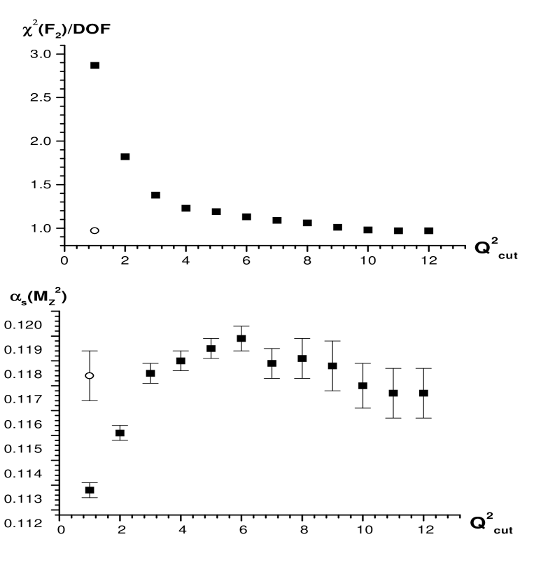
Figure 2: The values of $\alpha_{s}(M^{2}_{Z})$ and $\chi^{2}$ at different $Q^{2}$-values of data cutes in the fits based on nonsinglet evolution. The black points show the analyses of data without twist-four contributions. The white point corresponds to the case where twist-four contributions were added. Only statistical errors are shown.

The Table 7 contains the value of parameters of the twist-four term. As it was in the previous subsection, the twist-four terms for $H_{2}$ and $D_{2}$ data coincide with each other with errors taken into account that is in agreement with [14].

So, the analysis of combine SLAC, NMC, BCDMS and BFP data are given the following results:

• When HT corrections are not included and the cut of $Q^{2}$ is 10 GeV² at the free normalization

  $$\chi^{2}\mbox{/DOF}~{}=~{}0.98~{}~{}~{}\mbox{ and }~{}~{}~{}\alpha_{s}(90~{}\mbox{GeV}^{2}) = 0.1776\pm 0.0022~{}\mbox{(stat)},$$

  $$\alpha_{s}(M_{Z}^{2}) = 0.1170\pm 0.0009~{}\mbox{(stat)}$$ (53)

• When HT corrections are included and the cut of $Q^{2}$ is 1 GeV²

  $$\chi^{2}\mbox{/DOF}~{}=~{}0.97~{}~{}~{}\mbox{ and }~{}~{}~{}\alpha_{s}(90~{}\mbox{GeV}^{2}) = 0.1785\pm 0.0025~{}\mbox{(stat)},$$

  $$\alpha_{s}(M_{Z}^{2}) = 0.1174\pm 0.0010~{}\mbox{(stat)}$$ (54)

Thus, as it follows from nonsinglet fits of experimental data, perturbative QCD works rather well at $Q^{2}\geq 10$ GeV².

4.3.2. The study of threshold effects.

Here we would like to study threshold effects in $Q^{2}$-evolution of SF $F_{2}$. Note that at NLO level in nonsinglet case the coefficient function of $F_{2}$ and anomalous dimension do not depend on the number $n_{f}$ of active quarks. Then, the our study of the threshold effects in $Q^{2}$-evolution of SF $F_{2}$ is exactly equal to the investigation of a role of threshold effects in the QCD coupling constant $\alpha_{s}(Q^{2})$.

To study the threshold effects we consider two types of possible thresholds of heavy quarks: $Q^{2}_{f}=4m^{2}_{f}$ and $Q^{2}_{f}=m^{2}_{f}$. First type of thresholds has appeared when a heavy quark with the mass $m_{f}$ takes a possibility to be born. The second one lies close to the position of “Euclidean-reflected” threshold of heavy quarks. It should play a significant role (see [55]) in the $\alpha_{s}(Q^{2})$-evolution.

A.   Let thresholds appear at $Q^{2}_{f}=4m_{f}^{2}$. Then we split the range of the data to three separate ones:

• The $Q^{2}$ values are between $1$ GeV² and $10$ GeV², where the number $n_{f}$ of active quarks is $3$.

• The $Q^{2}$ values are between $10$ GeV² and $80$ GeV², where the number $n_{f}$ of active quarks is $4$.

• The $Q^{2}$ values are above $80$ GeV², where the number $n_{f}$ of active quarks is $5$.

Table 8. The values of $\alpha_{s}(M^{2}_{Z})$ and $\chi^{2}$ at different regimes of fits.

$N$ of	$Q^{2}$	$n_{f}$	$Q^{2}_{0}$	$N$ of	$\chi^{2}(F_{2})$	$\Lambda_{\overline{MS}}^{(3)}$	$\Lambda_{\overline{MS}}^{(4)}$	$\Lambda_{\overline{MS}}^{(5)}$	$\alpha_{s}(M^{2}_{Z})$
fit	range			points		$\pm$ stat	$\pm$ stat	$\pm$ stat	$\pm$ stat
						(MeV)	(MeV)	(MeV)
1	1-10	3	5	195	124	400 $\pm$ 30	308 $\pm$ 26	220 $\pm$ 23	0.1187 $\pm$ 0.0020
2	10-80	4	20	455	471		291 $\pm$ 17	208 $\pm$ 13	0.1177 $\pm$ 0.0012
3	80-300	5	90	190	143			199 $\pm$ 54	0.1169 $\pm$ 0.0040

The results are shown in Table 8. The average $\alpha_{s}(M^{2}_{Z})$ value can be calculated and it has the following value:

$$\alpha_{s}(M_{Z}^{2}) = 0.1178\pm 0.0010~{}\mbox{(stat)}$$ (55)

B.   Let thresholds appear at $Q^{2}_{f}=m_{f}^{2}$. Then we split the range of the data to two separate ones:

• The $Q^{2}$ values are between $2.5$ GeV² and $20.5$ GeV², where the number $n_{f}$ of active quarks is $4$.

• The $Q^{2}$ values are above $20.5$ GeV², where the number $n_{f}$ of active quarks is $5$.

Table 9. The values of $\alpha_{s}(M^{2}_{Z})$ and $\chi^{2}$ at different regimes of fits.

$N$ of	$Q^{2}$	$n_{f}$	$Q^{2}_{0}$	$N$ of	$\chi^{2}(F_{2})$	$\Lambda_{\overline{MS}}^{(4)}$	$\Lambda_{\overline{MS}}^{(5)}$	$\alpha_{s}(M^{2}_{Z})$
fit	range			points		$\pm$ stat	$\pm$ stat	$\pm$ stat
						(MeV)	(MeV)
1	2.5-20.5	4	10	241	197	298 $\pm$ 10	213 $\pm$ 8	0.1181 $\pm$ 0.0007
2	20.5-300	5	90	558	533		187 $\pm$ 16	0.1159 $\pm$ 0.0014

The results are shown in Table 9. The average $\alpha_{s}(M^{2}_{Z})$ value can be calculated and it has the following value:

$$\alpha_{s}(M_{Z}^{2}) = 0.1176\pm 0.0006~{}\mbox{(stat)}$$ (56)

Thus, we do not find a strong dependence on exact value of thresholds of heavy quarks. The theoretical uncertainties due to threshold effects can be estimated for $\alpha_{s}(M_{Z}^{2})$ as $0.0002$.

4.4 The results of the analyses based on nonsinglet evolution

Thus, using the analyses based on NS evolution of the SLAC, NMC, BCDMS and BFP experimental data for SF $F_{2}$ we obtain for $\alpha_{s}(M^{2}_{Z})$ the following expressions:

1. When we switch off the twist-four corrections, and put the cut $Q^{2}>10$ GeV², we have got at $\chi^{2}/DOF=0.98$

$$\alpha_{s}(M_{Z}^{2})~{}=~{}0.1170\pm 0.0009~{}\mbox{(stat)}\pm 0.0019~{}\mbox{(syst)}\pm 0.0010~{}\mbox{(norm)}$$ (57)

or

$$\alpha_{s}(M_{Z}^{2})~{}=~{}0.1170\pm 0.0023~{}\mbox{(total experimental error)}$$ (58)

2. When we add the twist-four corrections, and put the cut $Q^{2}>1$ GeV², we have got at $\chi^{2}/DOF=0.97$

$$\alpha_{s}(M_{Z}^{2})~{}=~{}0.1174\pm 0.0007~{}\mbox{(stat)}\pm 0.0021~{}\mbox{(syst)}\pm 0.0005~{}\mbox{(norm)}$$ (59)

or

$$\alpha_{s}(M_{Z}^{2})~{}=~{}0.1174\pm 0.0022~{}\mbox{(total experimental error)}$$ (60)

Looking at the results obtained in the Section we see that the central value of the coupling constant $\alpha_{s}(M_{Z}^{2})$ obtained in the fits (based on NS evolution) of combine SLAC, BCDMS, NM and BFP data lies between the central values of the coupling constants obtained separately in the fits of BCDMS data and in ones of SLAC, BCDMS, NM and BFP data. All obtained values of $\alpha_{s}(M_{Z}^{2})$ are in good agreement within existing statistical errors.

Figure 3: The study of systimatics at different $y_{cut}$ values in the fits based on combine siglet and nonsinglet evolution. The QCD analysis of BCDMS $C^{12},H_{2},D_{2}$ data (the case of combine evolution): no a $x_{cut}$, $Q_{0}^{2}=20$ GeV². Thresholds of $c$ and $b$ quarks are chosen at $Q^{2}=9$ GeV² and $Q^{2}=80$ GeV², respectively. The inner (outer) error-bars show statistical (systematic) errors.

5 Results of fits of $F_{2}$: the combined nonsinglet and
singlet evolution

At this case, the quite low $x$ experimental data lie at low $Q^{2}$ range and we choose $Q^{2}_{0}$ = 20 GeV². We use also $N_{max}=8$.

The study of the $N_{max}$-dependence of the results in the combine nonsinglet and singlet case of evolution has been found in [19]. Note here only that the analysis in [19] shows the $N_{max}$-independence of the obtained results starting already with $N_{max}=7$.

5.1 BCDMS $C^{12}+H_{2}+D_{2}$ data

As in the previous Section, we start our analyses with the experimental data [7, 8, 9] obtained by BCDMS muon scattering experiment. The full set of data is 762 points. The starting point of QCD evolution is $Q^{2}_{0}=20$ GeV².

Figure 4: The values of the slope $d(\ln{F_{2}})/d(\ln{Q^{2}})$ at $Q^{2}=20$ GeV². The white points correspond to the theoretical predictions based on combine singlet and nonsinglet evolution. The black points show BCDMS $C^{12}$, $H_{2}$ and $D_{2}$ data without a $Y_{cut}$.

Figure 5: Notation as in Fig. 4 with one exception: the $Y_{cut}$ with $N=5$ is taken into account.

As in the nonsinglet evolution case we have studied influence of the experimental systematic errors on the results of the QCD analysis as a function of $Y_{cut3}$, $Y_{cut4}$ and $Y_{cut5}$ applied to the data. Here we use also several sets $N$ of the values for the cuts at $0.5<x\leq 0.8$, which are given in the Table 10.

The absolute differences between the values of $\alpha_{s}$ for the distorted and undistorted sets of data are given in Table 11 and the Fig. 3 as the total systematic error of $\alpha_{s}$ estimated in quadratures. The number of the experimental points and the value of $\alpha_{s}$ for the undistorted set of $F_{2}$ are also given in the Table 11 and the Fig. 3.

Table 10. The values of $Y_{cut3}$, $Y_{cut4}$ and $Y_{cut5}$.

$N$	0	1	2	3	4	5
$Y_{cut3}$	0	0.14	0.16	0.18	0.22	0.23
$Y_{cut4}$	0	0.16	0.18	0.20	0.23	0.24
$Y_{cut5}$	0	0.20	0.20	0.22	0.24	0.25

Table 11. The values of $\alpha_{s}(M^{2}_{Z})$ at different values of $N$.

$N$	number	$\chi^{2}(F_{2})/DOF$	$\alpha_{s}(20~{}\mbox{GeV}^{2})$ $\pm$ stat	full
	of points			syst. error
0	762	1.22	0.1992 $\pm$ 0.0034	0.0122
1	649	1.06	0.2116 $\pm$ 0.0042	0.0096
2	640	1.07	0.2126 $\pm$ 0.0044	0.0088
3	627	1.05	0.2152 $\pm$ 0.0045	0.0080
4	596	1.04	0.2172 $\pm$ 0.0047	0.0076
5	590	1.04	0.2160 $\pm$ 0.0047	0.0068

From the Table 11 and the Fig. 3 we can see that the $\alpha_{s}$ values are obtained for $N=1\div 5$ of $Y_{cut3}$, $Y_{cut4}$ and $Y_{cut5}$ are very stable and statistically consistent. The case $N=5$ reduces the systematic error in $\alpha_{s}$ by factor $1.8$ and increases the value of $\alpha_{s}$, while increasing the statistical error on the 27%.

The importance of the $Y$-cut can be shown also in the Figs. 4 and 5, where the slope
$d(\ln{F_{2}})/d(\ln{Q^{2}})$ has been shown at $Q^{2}=20$ GeV². As we can see, there is an essential inprovement (the corresponding $\chi^{2}$(slope) decreases in half), when the $Y$-cut has been taken into account.

Figure 6: The values of the slope $d(\ln{F_{2}})/d(\ln{Q^{2}})$ at $Q^{2}=20$ GeV². The white points correspond to the theoretical predictions based on the twist-two approximation of perturbative QCD and combine singlet and nonsinglet evolution. The black points show SLAC, NMC and BFP experimental data.

Figure 7: Notation as in Fig. 6 with one exception: the target mass corrections are taken into account for theoretical predictions.

Figure 8: Notation as in Fig. 6 with one exception: the target mass and twist-four corrections are taken into account for theoretical predictions.

After the cuts have been implemented (in this Section below we use the set $N=5$), we have 590 points in the analysis. Fitting them in agreement with the same procedure considered in the Section 3, we obtain the following results:

$$\alpha_{s}(20~{}\mbox{GeV}^{2}) = 0.2160\pm 0.0047~{}\mbox{(stat)}\pm 0.0068~{}\mbox{(syst)}\pm 0.0031~{}\mbox{(norm)}$$

$$\alpha_{s}(M_{Z}^{2}) = 0.1175\pm 0.0014~{}\mbox{(stat)}\pm 0.0020~{}\mbox{(syst)}\pm 0.0011~{}\mbox{(norm)}$$

As in the nonsinglet case the last error ($\pm 0.0011$ to $\alpha_{s}(M_{Z}^{2})$) comes from difference in fits with free and fixed normalizations of BCDMS data [7, 8, 9] having different values of energy.

So, for the fits of BCDMS data [7, 8, 9] based on complete singlet and nonsinglet evolution with minimization of systematic errors, we have the following results (total experimental error is squared root of sum of squares of statistical error, systematic one and error of normalization):

$$\alpha_{s}(M_{Z}^{2})~{}=~{}0.1175\pm 0.0026~{}\mbox{(total experimental error)}$$ (62)

The value of $\alpha_{s}(M_{Z}^{2})$ corresponds to the following value of QCD mass parameter:

$$\Lambda^{(4)}_{\overline{\rm MS}} = \biggl{(}290\pm 20~{}\mbox{(stat)}\pm 29~{}\mbox{(syst)}\biggr{)}\mbox{ MeV},$$

$$\Lambda^{(5)}_{\overline{\rm MS}} = \biggl{(}206\pm 17~{}\mbox{(stat)}\pm 24~{}\mbox{(syst)}\biggr{)}\mbox{ MeV},$$ (63)

where the errors connected with the type of normalization of data are included already to systematic error.

5.2 SLAC and NMC $H_{2}+D_{2}$ data and BFP $Fe$ data

We continue our analyses with experimental data [4, 5, 6, 10] obtained by SLAC, NM and BFP Collaborations. The full set of data is 719 points (with the cut $Q^{2}>1$ GeV²): 364 ones of SLAC, 300 ones of NMC and 55 ones of BFP. The starting point of QCD evolution is $Q^{2}_{0}=20$ GeV².

As in previous Section we give an illustration of importance of $1/Q^{2}$ corrections. First of all, we analyze the data applying only perturbative QCD part of SF $F_{2}$, i.e. $F_{2}^{tw2}$. Later, we add the $1/Q^{2}$ corrections: firstly, target mass ones and later twist-four ones. As it is possible to see in the Table 12 and Figs. 6-8, we have the very bad fit ($\chi^{2}$(slope)$/DOF=40$), when we work only with twist-two part $F_{2}^{tw2}$. The agreement with the data is better essentially ($\chi^{2}$(slope)$/DOF\approx 9$) when target mass corrections have been added. The incorporation of twist-four corrections leads to very good fit of the data: $\chi^{2}$(slope)$/DOF\approx 1.05$ (see the Table 12 and the Fig. 8) . We note that the statistical and systematic errors are combined in quadratures.

Thus, we see that $\chi^{2}$(slope)$/DOF$ decreases in 38 times when the $1/Q^{2}$ corrections has been taken into account.

Table 12. The values of $\alpha_{s}(M^{2}_{Z})$ and $\chi^{2}$ at different regimes of fits.

$N$ of	TMC	HTC	syst.	$\chi^{2}(F_{2})/DOF$	$\chi^{2}(slope)$	$\alpha_{s}(20~{}\mbox{GeV}^{2})$	$\alpha_{s}(M^{2}_{Z})$
fits			error		for $23$ points	$\pm$ stat
1	No	No	Yes	5.5	800	0.2400 $\pm$ 0.0017	0.1241
2	Yes	No	Yes	2.2	179	0.2153 $\pm$ 0.0018	0.1174
3	Yes	Yes	Yes	0.85	21	0.2138 $\pm$ 0.0058	0.1170

Looking at the results in the Table 12, we see the following results for coupling constants

$$\alpha_{s}(20~{}\mbox{GeV}^{2}) = 0.2138\pm 0.0058~{}\mbox{(stat)}+\pm 0.0075~{}\mbox{(syst)}+0.0030\mbox{(norm)}$$

$$\alpha_{s}(M_{Z}^{2}) = 0.1170\pm 0.0016~{}\mbox{(stat)}+\pm 0.0021~{}\mbox{(syst)}+0.0011\mbox{(norm)}$$

As in the nonsinglet evolution fits, the last error $\pm 0.0011$ to $\alpha_{s}(M_{Z}^{2})$ comes from fits with free and fixed normalizations between different data of SLAC, NM and BFP Collaborations.

We would like to compare the results in the Table 12 with the results of the analyses of the data when an additional $W^{2}$-cut is taken into account. The inclusion of the $W^{2}$-cut is very popular (see [74] and references therein) and we fit considering data with variation of the $W^{2}$-cut (and with the standard cut $Q^{2}>1$ GeV²). The results of the fits (without twist-four correction) are presented in the Table 13 (the systematic errors of the data are included in the fits).

Table 13. The values of $\alpha_{s}(M^{2}_{Z})$ and $\chi^{2}$ in fits with different values of $W^{2}$-cut.

$N$ of	$W^{2}$	$\chi^{2}(F_{2})/DOF$	$\alpha_{s}(20~{}\mbox{GeV}^{2})$	$\Lambda_{\overline{MS}}^{(4)}$ (MeV)	$\Lambda_{\overline{MS}}^{(5)}$ (MeV)	$\alpha_{s}(M^{2}_{Z})$
fits	cut		$\pm$ stat	$\pm$ stat	$\pm$ stat	$\pm$ stat
1	2.0	1.30	0.2407 $\pm$ 0.0013	400 $\pm$ 6	296 $\pm$ 4	0.1243 $\pm$ 0.0004
2	4.0	1.00	0.2135 $\pm$ 0.0018	280 $\pm$ 7	194 $\pm$ 5	0.1169 $\pm$ 0.0004
3	6.0	1.00	0.2070 $\pm$ 0.0023	253 $\pm$ 9	178 $\pm$ 7	0.1150 $\pm$ 0.0007
4	8.0	0.91	0.2128 $\pm$ 0.0043	277 $\pm$ 18	197 $\pm$ 14	0.1167 $\pm$ 0.0012
5	10	0.91	0.2107 $\pm$ 0.0053	268 $\pm$ 22	190 $\pm$ 18	0.1162 $\pm$ 0.0015

As we can see from the Table 12 (the last line, where twist-four corrections are incorporated) and Table 13, the results for $\alpha_{s}(M^{2}_{Z})$ are in very good agreement for values of $W^{2}$-cut larger then 4 GeV². So, the $W^{2}$-cut procedure can be used successfully to switch off the range of experimental data where higher-twist corrections are required.

We would like to note that the results obtained in two previous subsections show very good agreement between the values of coupling constant $\alpha_{s}(M_{Z}^{2})$ obtained separately in the fits of BCDMS data and ones in the fits of combine SLAC, NMC and BFP data (see Eqs. (LABEL:bd1.b)-(63) and (LABEL:slo11.b)). Thus, as in the case of nonsinglet evolution we have possibility to fit togather all the data. It is the subject of the following subsection.

5.3 SLAC, BCDMS, NMC and BFP data

Here we start to analyze the maximal number of experimental points which have been produced in considered experiments. The full set of data is 1309 points.

5.3.1. The study of $Q^{2}$ range, where $1/Q^{2}$ corrections are important.

Here we would like to repeat our analysis given in Subsection 4.3 . Firstly we fit the data without a contribution of twist-four terms. We use the cut $Q^{2}\geq Q^{2}_{cut}$ and increase the value $Q^{2}_{cut}$ step by step. Later we do fits including the twist-four corrections and the cut $Q^{2}\geq 1$ GeV².

As it was in nonsinglet case, we observe very good agreement for first type of the fits starting with $Q^{2}_{cut}\geq 15$ GeV² (see the Table 14 and the Fig. 9). For the second type of fits the agreement is good already at $Q^{2}\geq 1$ GeV². The both types of the fits give very similar results. Moreover, the results are very close to ones obtained earlier in the nonsinglet case (see the Tables 3 and 6).

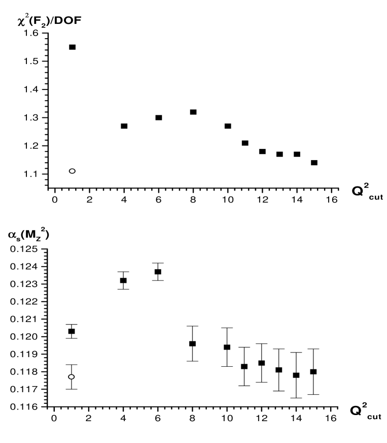
Figure 9: The values of $\alpha_{s}(M^{2}_{Z})$ and $\chi^{2}$ at different $Q^{2}$-values of data cutes in the fits based on combine singlet and nonsinglet evolution. The black points show the analyses of data without twist-four contributions. The white point corresponds to the case where twist-four contributions were added. Only statistical errors are shown.

Table 14. The values of $\alpha_{s}(M^{2}_{Z})$ and $\chi^{2}$ at different regimes of fits.

$N$ of	$Q^{2}$	$N$ of	HTC	$\chi^{2}(F_{2})$/DOF	$\alpha_{s}(20~{}\mbox{GeV}^{2})$	$\Lambda_{\overline{MS}}^{(4)}$	$\alpha_{s}(M^{2}_{Z})$
fits	cut	points			$\pm$ stat	(MeV)	$\pm$ stat
1	1.0	1309	No	1.55	0.2258 $\pm$ 0.0011	333	0.1203 $\pm$ 0.0004
2	4.0	1051	No	1.27	0.2364 $\pm$ 0.0017	380	0.1232 $\pm$ 0.0005
3	6.0	942	No	1.30	0.2385 $\pm$ 0.0022	390	0.1237 $\pm$ 0.0005
4	8.0	870	No	1.32	0.2232 $\pm$ 0.0035	321	0.1196 $\pm$ 0.0010
5	10.0	817	No	1.27	0.2226 $\pm$ 0.0035	318	0.1194 $\pm$ 0.0011
6	11.0	793	No	1.21	0.2187 $\pm$ 0.0038	301	0.1183 $\pm$ 0.0011
7	12.0	758	No	1.18	0.2192 $\pm$ 0.0039	304	0.1185 $\pm$ 0.0011
8	13.0	754	No	1.17	0.2180 $\pm$ 0.0039	297	0.1181 $\pm$ 0.0012
9	14.0	740	No	1.17	0.2169 $\pm$ 0.0041	294	0.1178 $\pm$ 0.0013
10	15.0	714	No	1.14	0.2177 $\pm$ 0.0042	297	0.1180 $\pm$ 0.0013
11	1.0	1309	Yes	1.11	0.2167 $\pm$ 0.0024	293	0.1177 $\pm$ 0.0007

Figure 10: The values of the slope $d(\ln{F_{2}})/d(\ln{Q^{2}})$ at $Q^{2}=20$ GeV². The white points correspond to the theoretical predictions based on perturbative QCD (with target mass corrections taken into account) and combine singlet and nonsinglet evolution. The black points show SLAC, BCDMS, NMC and BFP experimental data without a $Q^{2}$ cut.

Figure 11: Notation as in Fig. 10 with one exception: the cut $Q^{2}\geq 15$ GeV² is taken into account for experimental data.

Figure 12: Notation as in Fig. 10 with one exception: the twist-four corrections are taken into account for theoretical predictions.

We obtain the following results:

• When twist-four corrections are not included and the cut of $Q^{2}$ is 15 GeV²

  $$\chi^{2}\mbox{/DOF}~{}=~{}1.14~{}~{}~{}\mbox{ and }~{}~{}~{}\alpha_{s}(20~{}\mbox{GeV}^{2}) = 0.2177\pm 0.0042~{}\mbox{(stat)},$$

  $$\alpha_{s}(M_{Z}^{2}) = 0.1180\pm 0.0013~{}\mbox{(stat)}$$ (65)

• When twist-four corrections are included and the cut of $Q^{2}$ is 1 GeV²

  $$\chi^{2}\mbox{/DOF}~{}=~{}1.11~{}~{}~{}\mbox{ and }~{}~{}~{}\alpha_{s}(20~{}\mbox{GeV}^{2}) = 0.2167\pm 0.0024~{}\mbox{(stat)},$$

  $$\alpha_{s}(M_{Z}^{2}) = 0.1177\pm 0.0007~{}\mbox{(stat)}$$ (66)

For additional illustration of importance of $1/Q^{2}$ corrections at nonlarge $Q^{2}$ values we study the slope $d(\ln{F_{2}})/d(\ln{Q^{2}})$ as it has been done in the previous subsection 5.2 . First of all, we analyze the data applying only perturbative QCD approximation of SF $F_{2}$ (with target mass corrections taken into account), i.e. $F_{2}^{pQCD}$. Later, we add the cut $Q^{2}\geq 15$ GeV². As it is possible to see in the Figs. 10 and 11, we have the bad fit ($\chi^{2}$(slope)$/DOF\approx 7.78$) in the case without a $Q^{2}$ cut. The agreement with the data is strongly better when this $Q^{2}$ cut has been added: $\chi^{2}$(slope)$/DOF\approx 1.26$ in the case.

As in the previous subsection the incorporation of twist-four corrections leads also to very good fit of the data (without a $Q^{2}$ cut): $\chi^{2}$(slope)$/DOF\approx 1.09$ (see the Fig. 12) . These results demonstrate the importance of twist-four corrections at nonlarge $Q^{2}$ values.

Thus, as it follows from the fits of experimental data based on combine singlet and nonsinglet evolution, perturbative QCD works well at $Q^{2}\geq 15$ GeV².

5.3.2. The study of threshold effects.

Here we continue our study of threshold effects in $Q^{2}$-evolution of SF $F_{2}$. Note that at LO level and NLO one in the singlet case of evolution the coefficient functions of $F_{2}$ and anomalous dimensions depend on the number $n_{f}$ of active quarks.

By analogy with the NS case of evolution (see subsection 4.3.2), to study the threshold effects we consider two types of possible thresholds of heavy quarks: $Q^{2}_{f}=4m^{2}_{f}$ and $Q^{2}_{f}=m^{2}_{f}$. First type of thresholds has appeared when a heavy quark with the mass $m_{f}$ takes a possibility to be born (in the framework of photon-gluon fusion process, for example). The second one lies close to the position of “Euclidean-reflected” threshold of heavy quarks. It should play a significant role (see [55]) in the $\alpha_{s}(Q^{2})$-evolution.

A.   Let thresholds appear at $Q^{2}_{f}=4m_{f}^{2}$. Then we split the range of the data to three separate ones (see page 20).

Table 15. The values of $\alpha_{s}(M^{2}_{Z})$ and $\chi^{2}$ at different regimes of fits.

$N$ of	$Q^{2}$	$n_{f}$	$Q^{2}_{0}$	$N$ of	$\chi^{2}$	$\Lambda_{\overline{MS}}^{(3)}$	$\Lambda_{\overline{MS}}^{(4)}$	$\Lambda_{\overline{MS}}^{(5)}$	$\alpha_{s}(M^{2}_{Z})$
fit	range			points		$\pm$ stat	$\pm$ stat	$\pm$ stat	$\pm$ stat
						(MeV)	(MeV)	(MeV)
1	1-10	3	3.0	467	290	331 $\pm$ 24	250 $\pm$ 20	176 $\pm$ 16	0.1148 $\pm$ 0.0015
2	10-80	4	20	627	595		274 $\pm$ 21	194 $\pm$ 17	0.1165 $\pm$ 0.0014
3	80-300	5	90	190	156			220 $\pm$ 70	0.1187 $\pm$ 0.0050

The results are shown in Table 15. The average $\alpha_{s}(M^{2}_{Z})$ value can be calculated and it has the following value:

$$\alpha_{s}(M_{Z}^{2}) = 0.1158\pm 0.0010~{}\mbox{(stat)}$$ (67)

B.   Let thresholds appear at $Q^{2}_{f}=m_{f}^{2}$. Then we split the range of the data to two separate ones (see page 20).

Table 16. The values of $\alpha_{s}(M^{2}_{Z})$ and $\chi^{2}$ at different regimes of fits.

$N$ of	$Q^{2}$	$n_{f}$	$Q^{2}_{0}$	$N$ of	$\chi^{2}$	$\Lambda_{\overline{MS}}^{(4)}$	$\Lambda_{\overline{MS}}^{(5)}$	$\alpha_{s}(M^{2}_{Z})$
fit	range			points		$\pm$ stat	$\pm$ stat	$\pm$ stat
						(MeV)	(MeV)
1	2.5-20.5	4	10	519	396	230 $\pm$ 21	160 $\pm$ 16	0.1132 $\pm$ 0.0016
2	20.5-300	5	90	631	670		205 $\pm$ 15	0.1174 $\pm$ 0.0013

The results are shown in Table 16. The average $\alpha_{s}(M^{2}_{Z})$ value can be calculated and it has the following value:

$$\alpha_{s}(M_{Z}^{2}) = 0.1157\pm 0.0020~{}\mbox{(stat)}$$ (68)

The results are very surprising. From one side, all variables: the coefficient functions of $F_{2}$ and anomalous dimensions, depend on the number $n_{f}$ of active quarks. However, we do not find a strong dependence on exact value of thresholds of heavy quarks. From another side, the central values of the average $\alpha_{s}(M^{2}_{Z})$ obtained here are essentially lower than in other our analyses.

Thus, the theoretical uncertainties due to threshold effects can be estimated in the case of combine singlet and nonsinglet evolution for $\alpha_{s}(M_{Z}^{2})$ as $0.0001$.

5.3.3. The values of fitted parameters.

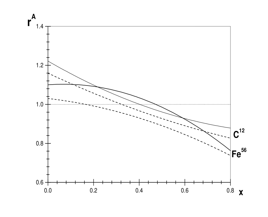
Figure 13: The values of the nuclear-effect ratio: $r^{A}$, for $A=C^{12}$ and $Fe^{56}$. The solid and dashen curvess correspond to the small-$x$ asymptotics $\sim x^{-\omega}$ of sea quark and gluon distributions with $\omega=0$ and $\omega=0.18$, respectively.

We have got the following values for parameters in parameterizations of parton distributions (at $Q^{2}_{0}=20$ GeV²) :

$$a_{u}(20) = 0.72,~{}~{}~{}~{}~{}~{}b_{u}(20)~{}=~{}3.72,$$

$$a_{d}(20) = 0.69,~{}~{}~{}~{}~{}~{}b_{d}(20)~{}=~{}5.81,$$

$$C_{S}(20) = 0.375,~{}~{}~{}~{}\,b_{S}(20)~{}=~{}13.8,$$

$$P_{G}(20) = 0.519,~{}~{}~{}~{}\,b_{G}(20)~{}=~{}11.4,$$

$$K_{1}^{C}(20) = 1.222,~{}~{}~{}K_{2}^{C}(20)~{}=~{}0.554,~{}~{}~{}~{}\,K_{3}^{C}(20)~{}=~{}0.253,$$

$$K_{1}^{F}(20) = 1.10,~{}~{}~{}~{}\,K_{2}^{F}(20)~{}=-0.081,~{}~{}\,K_{3}^{F}(20)~{}=-0.58$$ (69)

For the coefficients $a_{u}(20)$ and $a_{d}(20)$ we find good agreement between their values and the double-logarithmic estimations in Refs.[75, 76], based on [77]. We would like to note that the estimations in Ref. [75] have been given in other set of parameters that changes effectively only the value of normalization point $Q^{2}_{0}$. As it has been shown in Refs. [78, 42], the value of $a_{u}(20)$ and $a_{d}(20)$ should be nearly $Q^{2}$-independent (if the values are not too close to $1$) . This $Q^{2}$-independence of values of $a_{u}(20)$ and $a_{d}(20)$ explains our good agreement with the results of [75]. The values of $a_{u}(20)$ and $a_{d}(20)$ are supported also by recent fits (see discussions in Ref. [27]).

The value $b_{u}(20)$ is in agreement with Eqs.(48) and (52) and with other fits [12, 13, 26, 27], that supports its slow $Q^{2}$-dependence (see [73, 42]). The value of $b_{d}(20)$ is higher than $b_{u}(20)$ that is supported by other fits (see, for example, [12, 13]) and references therein) and by quark-counting rules [72]. The values of $b_{G}(20)$ and $b_{S}(20)$ are very high, that is in agreement with BCDMS analyses [7, 8, 9] and demonstrates difficulties to study the large-$x$ asymptotics of sea quark and gluon distributions in analyses of inclusive deep-inelastic data .

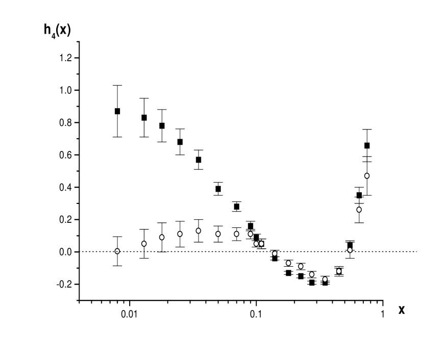
Figure 14: The values of the twist-four terms. The black and white points correspond to the small-$x$ asymptotics $\sim x^{-\omega}$ of sea quark and gluon distributions with $\omega=0$ and $\omega=0.18$, respectively. The statistical errors are displayed only.

The value of $P_{G}(20)$ shows that at $Q^{2}_{0}=20$ GeV² gluons contain about half of nucleon momentum.

The coefficients $K^{C}_{i}(20)$ and $K^{F}_{i}(20)$ ($i=1,2,3$) demonstrate non-zero values of nuclear effects for bound nucleons in $C^{12}$ and $Fe$ nuclei. The Eqs. (39) with the values of coefficients $K^{C}_{i}(20)$ and $K^{F}_{i}(20)$ given in Eqs. (69) demonstrate the shapes of nuclear effects which are represented in Fig 3, where we see a resonable agreement of our curves with the experimental data from Refs [57, 60].

The values of twist-four terms are given in the Table 17. To obtain the values we used the approximate equality of twist-four terms for $H_{2}$ and $D_{2}$ targets that has been obtained in our studies in the previous Section (see the Tables 5 and 7). This is also in agreement with the Ref. [14]. The values of twist-four terms are represented also in Fig. 14.

We would like to note (see the Table 17 and Fig. 14) about a quite strong rise of twist-four terms at lower $x$-bins. The necessity of large magnitude of twist-four corrections at the low $x$ values it is possible to observe also in the Figs. 6, 7 and 10, where there is a quite strong difference between experimental data and theoretical predictions (based on perturbative QCD) for the slope $d(\ln{F_{2}})/d(\ln{Q^{2}})$. The rise is in good agreement with theoretical predictions [84] and with the recent analyses of H1 and ZEUS data at low values of $x$ and $Q^{2}$ (see [33]).

Table 17. The values of the twist-four terms.

$x_{i}$	$\tilde{h}_{4}(x_{i})$	$x_{i}$	$\tilde{h}_{4}(x_{i})$	$x_{i}$	$\tilde{h}_{4}(x_{i})$
	$\pm$ stat		$\pm$ stat		$\pm$ stat
0.008	0.87 $\pm$ 0.16	0.090	0.16 $\pm$ 0.03	0.275	-0.19 $\pm$ 0.01
0.013	0.83 $\pm$ 0.12	0.100	0.09 $\pm$ 0.02	0.350	-0.19 $\pm$ 0.01
0.018	0.78 $\pm$ 0.10	0.110	0.05 $\pm$ 0.03	0.450	-0.12 $\pm$ 0.02
0.025	0.68 $\pm$ 0.08	0.140	-0.04 $\pm$ 0.01	0.500	0.45 $\pm$ 0.23
0.035	0.57 $\pm$ 0.06	0.150	0.43 $\pm$ 0.11	0.550	0.04 $\pm$ 0.03
0.050	0.39 $\pm$ 0.04	0.180	-0.13 $\pm$ 0.01	0.650	0.35 $\pm$ 0.05
0.070	0.28 $\pm$ 0.03	0.225	-0.15 $\pm$ 0.01	0.750	0.66 $\pm$ 0.10
0.080	0.30 $\pm$ 0.15	0.250	-0.27 $\pm$ 0.13

5.3.4. BFKL-like parameterizations of gluon and sea quark distributions.

As we have already discussed in Section 2, we would like to try to study the parameters of the sea quark and gluon distributions when the terms $\sim x^{a_{S}(Q^{2}_{0})}$ and $\sim x^{a_{G}(Q^{2}_{0})}$ were incorporated. These terms take into account a possible rise of the sea quark and gluon distributions at low $x$ values. As it has been already noted in Section 2, from DGLAP-like analyses [80, 47, 48], the parameters $a_{S}$ and $a_{G}$ should be the same, because they are mixed together into the “$+$”-component of the $Q^{2}$-evolution (see [47]). Moreover, the parameter $\omega=-a_{S}=-a_{G}$ should be $Q^{2}$-independent (see, for example, [80, 48]), if it is not small, i.e. $x^{-\omega}>>Const$ at small $x$.

In the fit with free nonzero $\omega$ value we have got the following values for parameters in parameterizations of parton distributions (at $Q^{2}_{0}=20$ GeV²) :

$$a_{u}(20) = 0.72,~{}~{}~{}~{}~{}~{}~{}b_{u}(20)~{}=~{}3.69,$$

$$a_{d}(20) = 0.68,~{}~{}~{}~{}~{}~{}~{}b_{d}(20)~{}=~{}5.44,$$

$$a_{S}(20) = -0.18,~{}~{}~{}~{}a_{G}(20)~{}=~{}-0.18,$$

$$C_{S}(20) = 0.185,~{}~{}~{}~{}~{}\,b_{S}(20)~{}=~{}10.4,$$

$$P_{G}(20) = 0.524,~{}~{}~{}~{}~{}b_{G}(20)~{}=~{}7.31,$$

$$K_{1}^{C}(20) = 1.160,~{}~{}~{}\,K_{2}^{C}(20)~{}=~{}0.472,~{}~{}\,K_{3}^{C}(20)~{}=~{}0.141,$$

$$K_{1}^{F}(20) = 1.03,~{}~{}~{}~{}~{}K_{2}^{F}(20)~{}=~{}0.131,~{}~{}\,K_{3}^{F}(20)~{}=~{}-0.28$$ (70)

We would like to note that the values of parameters of valent quark distributions are not changed really. The values of $b_{G}(20)$ and $b_{S}(20)$ are yet high but they are closer to predictions of quark-counting rules [72] than the corresponding values obtained in the previous subsection.

The values of the parameters of the nuclei effect ratio are not changed within considered errors. The similarity of the results for the nuclei effect ratio is shown in the Fig. 13.

The value of $\omega$ is equal to $0.18$, that is in perfect agreement with the recent studies based on BFKL dynamics [85] when NLO corrections [86, 87] were taken into account (see, for example, studies [88], a review [89] and references therein). Moreover, this value is in good agreement also with recent phenomenological studies (see a recent review in [90]) of Pomeron intercept values and also with recent H1 and L3 data [43, 91].

As it is possible to see in the Tables 17 and 18 and also in Fig. 14, the effect of strong rise of twist-four magnitude at small $x$ values observed in previous subsection is completely absent here . So, the rise is replaced by the small $x$ rise of twist-two gluon and sea quark distributions. This replacement seems due to a small number of experimental points at low $x$ range and narrow range of $Q^{2}$ values there. The cancellation of twist-four corrections at low $x$ is in good agreement with the recent studies [32, 92]. This demonstrates the fact that a strong rise of twist-four corrections coming from BFKL-like approaches [84] has negligible magnitude (see [92, 33]).

Table 18. The values of the twist-four terms.

$x_{i}$	$\tilde{h}_{4}(x_{i})$	$x_{i}$	$\tilde{h}_{4}(x_{i})$	$x_{i}$	$\tilde{h}_{4}(x_{i})$
		$\pm$ stat	$\pm$ stat		$\pm$ stat
0.008	0.004 $\pm$ 0.090	0.090	0.11 $\pm$ 0.03	0.275	-0.14 $\pm$ 0.02
0.013	0.05 $\pm$ 0.09	0.100	0.05 $\pm$ 0.02	0.350	-0.17 $\pm$ 0.02
0.018	0.09 $\pm$ 0.09	0.110	0.05 $\pm$ 0.03	0.450	-0.12 $\pm$ 0.03
0.025	0.11 $\pm$ 0.08	0.140	-0.01 $\pm$ 0.02	0.500	0.43 $\pm$ 0.23
0.035	0.13 $\pm$ 0.07	0.150	0.62 $\pm$ 0.12	0.550	0.01 $\pm$ 0.05
0.050	0.11 $\pm$ 0.05	0.180	-0.07 $\pm$ 0.02	0.650	0.26 $\pm$ 0.08
0.070	0.11 $\pm$ 0.04	0.225	-0.09 $\pm$ 0.02	0.750	0.47 $\pm$ 0.12
0.080	0.31 $\pm$ 0.16	0.250	-0.16 $\pm$ 0.14

The value of $\alpha_{s}(M_{Z}^{2})$ in the fit (with the number of points $N=1309$ and $\chi^{2}/DOF=1.1$) is as follows:

$$\alpha_{s}(M_{Z}^{2})~{}=~{}0.1187\pm 0.0015~{}\mbox{(stat)},$$ (71)

i.e. it is in good agreement within statistical errors with fits performed earlier but the middle value is slightly higher.

5.4 The results of analyses with combine singlet and nonsinglet evolution

Thus, using singlet analyses of the SLAC, NMC, BCDMS and BFP experimental data for SF $F_{2}$ we obtain for $\alpha_{s}(M^{2}_{Z})$ the following expression:

$$\alpha_{s}(20~{}\mbox{GeV}^{2}) = 0.2167\pm 0.0024~{}\mbox{(stat)}\pm 0.0080~{}\mbox{(syst)}\pm 0.0012~{}\mbox{(norm)}$$

$$\alpha_{s}(M_{Z}^{2}) = 0.1177\pm 0.0007~{}\mbox{(stat)}\pm 0.0021~{}\mbox{(syst)}\pm 0.0005~{}\mbox{(norm)}$$

Looking at the results obtained in the Sections we see very good agreement between the value of coupling constant $\alpha_{s}(M_{Z}^{2})$ obtained in the fits of combine SLAC, BCDMS, NMC and BFP data and the values of $\alpha_{s}(M_{Z}^{2})$ obtained separately in the fits of BCDMS data and in ones of SLAC, BCDMS, NMC and BFP data.

6 The dependence on factorization and renormalization scales

In the section we study the dependence of our results on the different choice of the factorization scale $\mu_{F}$ and the renormalization one $\mu_{R}$. Following the studies [14, 36] we choose three following values ($1/2,~{}1,~{}2$) for the coefficients $k_{F}$ and $k_{R}$.

6.1 Nonsinglet evolution case

The results are given in the Table 19. We do fits here without higher-twist corrections (no HTC), with the number of points $596$, at $Q^{2}>10.5$ GeV² and for free normalization of different sets of data. The change of the value of coupling constant $\alpha_{s}(M^{2}_{Z})$ at some $k_{F}$ and $k_{R}$ values is denoted by the difference:

$$\Delta\alpha_{s}(M_{Z}^{2})~{}=~{}\alpha_{s}(M_{Z}^{2})-\alpha_{s}(M_{Z}^{2})|_{k_{F}=k_{R}=1}$$ (73)

Table 19. The values of $\alpha_{s}(M^{2}_{Z})$ at different values of $k_{F}$ and $k_{R}$. The values in brackets correspond to the case when the Eq.(22) replaces the Eq.(20) into the NLO corrections to coefficient functions.

$k_{R}$	$k_{F}$.	$\chi^{2}(F_{2})$	$\alpha_{s}(90~{}\mbox{GeV}^{2})$ $\pm$ stat	$\alpha_{s}(M^{2}_{Z})$	$\Delta\alpha_{s}(M_{Z}^{2})$
1	1	556	0.1789 $\pm$ 0.0023	0.1175	0
1/2	1	558	0.1769 $\pm$ 0.0022	0.1167	$-$0.0008
			(0.1745)	(0.1155)	($-$0.0020)
1	1/2	545	0.1730 $\pm$ 0.0021	0.1150	$-$0.0025
1	2	568	0.1876 $\pm$ 0.0025	0.1211	+0.0036
2	1	555	0.1826 $\pm$ 0.0025	0.1191	+0.0016
			(0.1858)	(0.1203)	(+0.0028)
1/2	2	570	0.1856 $\pm$ 0.0026	0.1203	+0.0028
			(0.1817)	(0.1186)	(+0.0011)
2	1/2	554	0.1770 $\pm$ 0.0022	0.1167	$-$0.0008
			(0.1784)	(0.1173)	($-$0.0002)
1/2	1/2	556	0.1789 $\pm$ 0.0023	0.1175	$-$0.0034
			(0.1694)	(0.1134)	($-$0.0041)
2	2	567	0.1912 $\pm$ 0.0028	0.1225	+0.0050
			(0.1965)	(0.1245)	(+0.0070)

We find similar variation of $\alpha_{s}(M^{2}_{Z})$ with the variations of $k_{F}$ and $k_{R}$: $\alpha_{s}(M^{2}_{Z})$ increases (falls) with increasing (decreasing) of values of $k_{F}$ and/or $k_{R}$. So, the dependence is quite similar to one which has been obtained in [39, 26, 27] by the variation of $k$-scale from $1/4$ to $4$ ($k\equiv k_{F}=k_{R}$ in [39, 26, 27]).

Taking maximal and minimal values (that corresponds to $k_{R}=k_{F}=1/2$ and $2$, respectively) of coupling constant we obtain the theoretical uncertainties $+0.0050$ and $-0.0034$ for $\alpha_{s}(M^{2}_{Z})$. In the case when the replacement (22) has been used also in NLO corrections to the coefficient functions (i.e. when the Eq.(22) replaces the Eq.(20) there), the theoretical uncertainties for $\alpha_{s}(M^{2}_{Z})$ are little higher: $+0.0070$ and $-0.0041$.

Thus, using the analyses with NS evolution of the SLAC, NMC, BCDMS and BFP experimental data for SF $F_{2}$ we obtain for $\alpha_{s}(M^{2}_{Z})$ the following expressions (when no HTC, $Q^{2}>10$ GeV² and $\chi^{2}=0.98$):

$$\alpha_{s}(M_{Z}^{2})~{}=~{}0.1170\pm 0.0009~{}\mbox{(stat)}\pm 0.0019~{}\mbox{(syst)}\pm 0.0010~{}\mbox{(norm)}+~{}\biggl{\{}\begin{array}[]{l}+0.0050\\ -0.0034\end{array}~{}\mbox{(theor)},$$ (76)

or

$$\alpha_{s}(M_{Z}^{2})~{}=~{}0.1170\pm 0.0023~{}\mbox{(total experimental error)}+~{}\biggl{\{}\begin{array}[]{l}+0.0050\\ -0.0034\end{array}~{}\mbox{(theor)},$$ (79)

where the symbol theor marks the theoretical uncertainties which contain the sum of the scale uncertainties, threshold error ($\pm 0.0002$) and the method error ($\pm 0.0002$) in quadratures.

6.2 Combine singlet and nonsinglet evolution

The results are given in the Table 20. We do fits with higher-twist corrections, with the number of points $1309$, at $Q^{2}>1$ GeV² and for free normalization of different sets of data.

Table 20.  The values of $\alpha_{s}(M^{2}_{Z})$ at different values of $k_{F}$ and $k_{R}$. The values in brackets correspond to the case when the Eq.(22) replaces the Eq.(20) into the NLO corrections to coefficient functions.

$k_{R}$	$k_{F}$.	$\chi^{2}(F_{2})$	$\alpha_{s}(20~{}\mbox{GeV}^{2})$ $\pm$ stat	$\Lambda^{(4)}_{\overline{\rm MS}}$	$\Lambda^{(5)}_{\overline{\rm MS}}$	$\alpha_{s}(M^{2}_{Z})$	$\Delta\alpha_{s}(M^{2}_{Z})$
				MeV	MeV
1	1	1410	0.2167 $\pm$ 0.0024	293	209	0.1178	0
1/2	1	1410	0.2112 $\pm$ 0.0019	270	191	0.1162	$-$0.0016
		(1443)	(0.2104 $\pm$ 0.0029)	(267)	(189)	(0.1160)	($-$0.0018)
1	1/2	1423	0.2040 $\pm$ 0.0020	241	168	0.1140	$-$0.0038
1	2	1447	0.2300 $\pm$ 0.0031	351	256	0.1215	+0.0037
2	1	1413	0.2204 $\pm$ 0.0024	309	222	0.1189	+0.0011
		(1500)	(0.2263 $\pm$ 0.0030)	(334)	(242)	(0.1204)	(+0.0026)
1/2	2	1422	0.2190 $\pm$ 0.0029	303	217	0.1185	$+$0.0007
		(1500)	(0.2132 $\pm$ 0.0031)	(278)	(197)	(0.1167)	($-$0.0011)
2	1/2	1460	0.2021 $\pm$ 0.0022	233	162	0.1134	$-$0.0044
		(1496)	(0.2323 $\pm$ 0.0030)	(361)	(264)	(0.1220)	(+0.0042)
1/2	1/2	1436	0.1975 $\pm$ 0.0012	216	149	0.1120	$-$0.0058
		(1450)	(0.1970 $\pm$ 0.0018)	(214)	(148)	(0.1120)	($-$0.0058)
2	2	1447	0.2340 $\pm$ 0.0033	369	271	0.1225	+0.0047
		(1460)	(0.2343 $\pm$ 0.0032)	(370)	(271)	(0.1226)	(+0.0048)

We find that variations of $\alpha_{s}(M^{2}_{Z})$ with the variations of $k_{F}$ and $k_{R}$ are very similar to ones which have been obtained in previous subsection. However, there is a quite big difference in the cases $k_{R}=2$, $k_{F}=1/2$ and $k_{R}=1/2$, $k_{F}=2$ between results in the Table 20 in brackets and without ones. The difference seems to come from the correlations between the values of higher-order contributions (that is mimicked by scale dependences) and twist-four corrections, i.e. so-called duality effect (see [27] and references therein).

As in the case of nonsinglet evolution, the dependence of $\alpha_{s}(M^{2}_{Z})$ with the variations of $k_{F}$ and $k_{R}$ is quite similar to one which have been obtained in [39] by the variation of $k_{R}$-scale from $1/4$ to $4$.

Taking maximal and minimal values (that corresponds to $k_{R}=k_{F}=1/2$ and $2$, respectively) of coupling constant we obtain the theoretical errors $+0.0050$ and $-0.0057$ for $\alpha_{s}(M^{2}_{Z})$. In the case when the replacement (22) has been used also in NLO corrections to the coefficient functions (i.e. when the Eq.(22) replaces the Eq.(20) there) the theoretical uncertainties for $\alpha_{s}(M^{2}_{Z})$ are changed very little but $\chi^{2}(F_{2})$ is higher.

Thus, using these analyses of the SLAC, NMC, BCDMS and BFP experimental data for SF $F_{2}$ we obtain for

$$\alpha_{s}(M_{Z}^{2})=0.1177\pm 0.0007~{}\mbox{(stat)}\pm 0.0021~{}\mbox{(syst)}\pm 0.0005~{}\mbox{(norm)}+~{}\biggl{\{}\begin{array}[]{l}+0.0047\\ -0.0057\end{array}~{}\mbox{(theor)},$$ (82)

where the theoretical uncertainties contain the scale ones (see above), the ones due to threshold effects ($\pm 0.0001$) and the method error ($\pm 0.0002$) in quadratures.

In conclusion of the Section we would like to note that the theoretical uncertainties in both types of analyses (based on nonsinglet evolution and on combined singlet and nonsinglet one) are essentially larger than the corresponding total experimental errors.

Indeed, the total experimental errors are as follows:
in the analyses with the nonsinglet evolution:

$$\mbox{(total experimental error)}~{}=~{}$$

$$\biggl{\{}\begin{array}[]{ll}~{}\mbox{(stat)}+\mbox{(syst)}+\mbox{(norm)}~{}=~{}0.0038&\mbox{(total linear experimental error)}\\ \sqrt{~{}\mbox{(stat)}^{2}+\mbox{(syst)}^{2}+\mbox{(norm)}^{2}}~{}=~{}0.0023&\mbox{(total quadratic experimental error)}\end{array}$$ (85)

in the analyses with the combined singlet and nonsinglet evolution:

$$\mbox{(total experimental error)}~{}=~{}\biggl{\{}\begin{array}[]{ll}0.0033&\mbox{(total linear experimental error)}\\ 0.0023&\mbox{(total quadratic experimental error)},\end{array}$$ (88)

i.e. they are less by factor $1.5\div 2$ to compare with corresponding theoretical uncertainties.

As it has been shown in [39, 40, 26, 27], the theoretical uncertainties decrease essentially (by a factor around $2.5$), when NNLO corrections have been taken into account. So, the fits of combined data show real necessity in analyses of DIS data at NNLO approximation.

7 Summary

As a conclusion, we would like to stress again, that using the Jacobi polynomial expansion method, developed in [17, 18, 19], we have studied the $Q^{2}$-evolution of DIS structure function $F_{2}$ fitting all modern experimental data existing at values of Bjorken variable $x$: $x\geq 10^{-2}$.

1. From the fits we have obtained the value of the normalization $\alpha_{s}(M^{2}_{Z})$ of QCD coupling constant. First of all, we have reanalyzed the BCDMS data cutting the range with large systematic errors. As it is possible to see in subsections 4.1 and 5.1 (and also the Figs. 1 and 3), the values of $\alpha_{s}(M^{2}_{Z})$ rise strongly when the cuts of systematics were incorporated. In another side, the values of $\alpha_{s}(M^{2}_{Z})$ does not dependent on the concrete type of the cut within modern statistical errors.

The values $\alpha_{s}(M^{2}_{Z})$ obtained in various fits are in good agreement with one other. Indeed, we have very similar results for $\alpha_{s}(M^{2}_{Z})$ in separate analyses of BCDMS data (with the cuts of systematics) and other ones. This gives us the possibility to fit all data together.

We have found that at $Q^{2}\geq 10\div 15$ GeV² the formulae of pure perturbative QCD (i.e. twist-two approximation together with target mass corrections) are in good agreement with all data. The results for $\alpha_{s}(M^{2}_{Z})$ are very similar for the both types of analyses: ones, based on nonsinglet evolution, and ones, based on combined singlet and nonsinglet evolution. They have the following form:

from fits, based on nonsinglet evolution:

$$\alpha_{s}(M_{Z}^{2}) = 0.1170\pm 0.0009~{}\mbox{(stat)}\pm 0.0019~{}\mbox{(syst)}\pm 0.0010~{}\mbox{(norm)},$$

from fits, based on combined singlet and nonsinglet evolution:

$$\alpha_{s}(M_{Z}^{2}) = 0.1180\pm 0.0013~{}\mbox{(stat)}\pm 0.0021~{}\mbox{(syst)}\pm 0.0009~{}\mbox{(norm)},$$ (90)

When we have added twist-four corrections, we have very good agreement between QCD (i.e. first two coefficients of Wilson expansion) and data starting already with $Q^{2}=1$ GeV², where the Wilson expansion should begin to be applicable. The results for $\alpha_{s}(M^{2}_{Z})$ coincide for the both types of analyses: ones, based on nonsinglet evolution, and ones, based on combined singlet and nonsinglet evolution. They have the following form:

from fits, based on nonsinglet evolution:

$$\alpha_{s}(M_{Z}^{2}) = 0.1174\pm 0.0007~{}\mbox{(stat)}\pm 0.0019~{}\mbox{(syst)}\pm 0.0010~{}\mbox{(norm)},$$

from fits, based on combined singlet and nonsinglet evolution:

$$\alpha_{s}(M_{Z}^{2}) = 0.1177\pm 0.0007~{}\mbox{(stat)}\pm 0.0021~{}\mbox{(syst)}\pm 0.0009~{}\mbox{(norm)},$$ (92)

Thus, there is very good agreement (see Eqs. (7), (90), (7) and (7)) between results based on pure perturbative QCD at quite large $Q^{2}$ values (i.e. at $Q^{2}\geq 10\div 15$ GeV²) and the results based on first two twist terms of Wilson expansion (at $Q^{2}\geq 1$ GeV², where the Wilson expansion should be applicable).

We would like to note that we have good agreement also with the analysis [69] of combined H1 and BCDMS data, which has been given by H1 Collaboration very recently. The shapes of twist-four corrections are very similar to ones from [14, 93]. Our results for $\alpha_{s}(M_{Z}^{2})$ are in good agreement also with the average value for coupling constant, presented in the recent studies (see [26, 39, 40, 65, 74, 94, 95] and references therein) and in famous Bethke review [96].

2. As the second item of our summary we would like to note about the real importance of NNLO corrections in analyses of DIS experimental data. The incorporation of the NNLO corrections have been started already several years ago in various ways (see Introduction for discussions).

The results are based on the studies of the effect of high order corrections, which can be estimated from the dependence of our results on factorization scale $\mu_{F}$ and renormalization one $\mu_{R}$. As it has been point out already in the previous Section the value of the theoretical uncertainties , coming from this dependence of the results for $\alpha_{s}(M_{Z}^{2})$ (given by Eqs.(76) and (82) for two types of $Q^{2}$-evolution), are equal to

$$\Delta\alpha_{s}(M_{Z}^{2})|_{\mbox{theo}}~{}=~{}\biggl{\{}\begin{array}[]{l}+0.0047\\ -0.0057\end{array}$$ (95)

Thus, the theoretical uncertainties are higher essentially than the total experimental error (88). Similar values of the theoretical error can be found in recent analyses of DIS process (see [39, 40, 26]) and of $e^{+}e^{-}$-process in [94, 95]. As it has been studied recently by van Neerven and Vogt [39, 40], the value of theoretical error decreases strongly (by a factor around 2.5) when the NNLO corrections have been taken into account. Thus, our fits of combined data performed here and also other analyses [94, 95] show real necessity to include the NNLO corrections to the study of DIS experimental data.

As it has been noted in Introduction, using partial information about NNLO QCD corrections several fits of experimental data have been performed (see [22]-[27], [39, 40, 65, 97] and references therein). In order to do the analyses of experimental data in full range of $x$ values, it is necessary to know exactly all NNLO QCD corrections. At present three-loop corrections to anomalous dimensions of Wilson operators are still unknown. These calculations, which are known only for several finite number of fixed Mellin moments [98], will be performed [99] in nearest future by using modern approaches (see [37, 100, 99]) to evaluate complicated Feynman diagrams.

3. At the end of our paper we would like to discuss the contributions of higher twist corrections.

In our study here we have reproduced well-known $x$-shape of the twist-four corrections at the large and intermediate values of Bjorken variable $x$ (see, for example, the Tables 5, 7 and 17 and also, for example, the results of very popular article [14]).

We would like to note about a small-$x$ rise of the magnitude of twist-four corrections, when we use flat parton distributions at $x\to 0$. The rise is in full agreement with the theoretical predictions [84]. As we have discussed already in the Section 5, there is a strong correlation between the small-$x$ behavior of twist-four corrections and the type of the corresponding asymptotics of the leading-twist parton distributions. The possibility to have a singular type of the asymptotics leads (in our fits) to the appearance of the rise of sea quark and gluon distributions as $\sim x^{-0.18}$ at low $x$ values. At this case the rise of the magnitude of twist-four corrections is completely canceled. This cancellation is in full agreement with theoretical and phenomenological studies and low $x$ experimental data of H1 and L3 Collaborations (see discussions in subsection 5.3.4).

We would like also to give a few words concerning the IRR-model predictions for the twist-four and twist-six corrections.

In our previous study [21] based on the IRR-model predictions for higher twist corrections, we have found a strong correlations between these corrections and the value of coupling constant. The $\alpha_{s}(M_{Z}^{2})$ value tends to be very small: $\alpha_{s}(M_{Z}^{2})=0.103\pm 0.002~{}\mbox{(stat)}$. This study has been supported by fits of DELPHI Collaboration (see [101]) and by some other analyses [95]. There is, however, a disagreement with the results of the paper [102], where the twist-four corrections in the framework of the IRR-model do not lead to decrease the $\alpha_{s}(M_{Z}^{2})$ value. In our opinion, the situation is not so clear here and it needs more investigations. We hope to return to this problem in our future studies.

References

-
[1]
M. Maul, E. Stein, L. Mankiewicz, M. Meyer-Hermann,
and A. Schaffer,
Phys.Lett. B401 (1997) 100; hep-ph/9710392;
V.M. Braun, Preprint NORDITA 97/53-P (hep-ph/9708386);
B.R. Webber, Nucl.Phys.Proc.Suppl. B71 (1999) 66. -
[2]
M. Beneke, Phys.Report. 317 (1999) 1;
M. Beneke and V.M. Braun, Preprint PITHA-00-25, TPR-00-19 (hep-ph/0010208). - [3] W.J. Stirling, Summary of Structure Function section on DIS2001.
- [4] SLAC Collab., L.W. Whitlow et al., Phys. Lett. B282 (1992) 475.
- [5] SLAC Collab., L.W. Whitlow, Ph.D. Thesis Standford University, SLAC report 357 (1990).
- [6] NM Collab., M. Arneodo et al., Nucl. Phys. B483 (1997) 3.
- [7] BCDMS Collab., A.C. Benevenuti et al., Phys. Lett. B223 (1989) 485; Preprint CERN-EP/89-06.
- [8] BCDMS Collab., A.C. Benevenuti et al., Phys. Lett. B237 (1990) 592; Preprint CERN-EP/89-170.
- [9] BCDMS Collab., A.C. Benevenuti et al., Phys. Lett. B195 (1987) 91; Preprint CERN-EP/87-100.
- [10] BFP Collab.: P.D. Mayers et al., Phys. Rev. D34 (1986) 1265.
- [11] A.B. Bukhvostov, E.A. Kuraev, and L.N. Lipatov, Sov. J. Nucl. Phys. 38 (1983) 439; A.B. Bukhvostov, V.S. Fadin, E.A. Kuraev, and L.N. Lipatov, Nucl. Phys. B258 (1985) 601.
- [12] S. I. Alekhin, Eur. Phys. J. C10 (1999) 395.
- [13] S. I. Alekhin, Phys. Rev. D63 (2001) 094022.
- [14] M. Virchaux and A. Milsztajn, Phys. Lett. B274 (1992) 221.
-
[15]
A.D. Martin, R.G. Roberts, W.J. Stirling and R.S. Thorne,
Eur. Phys. J. C14 (2000) 155;
M. Glueck, E. Reya and A. Vogt, Eur. Phys. J. C5 (1998) 4611;
STEQ Collab., H.Lai et al., Eur. Phys. J. C12 (2000) 375. -
[16]
V.N. Gribov and L.N. Lipatov, Sov. J. Nucl. Phys.
15 (1972) 438;
L.N. Lipatov, Sov. J. Nucl. Phys. 20 (1975) 94;
G. Altarelli and G. Parisi, Nucl. Phys. B126 (1977) 298;
Yu.L. Dokshitzer, JETP 46 (1977) 641. -
[17]
G. Parisi and N. Sourlas, Nucl. Phys. B151 (1979) 421
I.S. Barker, C.B. Langensiepen and G. Shaw, Nucl. Phys. B186 (1981) 61
I.S. Barker, B.R. Martin, and G. Shaw, Z. Phys. C19 (1983) 147
I.S. Barker and B.R. Martin, Z. Phys. C24 (1984) 255. - [18] V.G. Krivokhizhin, S.P. Kurlovich, V.V. Sanadze, I.A. Savin, A.V. Sidorov and N.B. Skachkov, Z. Phys. C36 (1987) 51.
- [19] V.G. Krivokhizhin, S.P. Kurlovich, R. Lednicky, S. Nemechek, V.V. Sanadze, I.A. Savin, A.V. Sidorov and N.B. Skachkov, Z. Phys. C48 (1990) 347.
-
[20]
V.I. Vovk, Z. Phys. C47 (1990) 57;
A.V. Kotikov, G. Parente and J. Sanchez Guillen, Z. Phys. C58 (1993) 465. - [21] A.V. Kotikov and V.G. Krivokhijine, in Proceedings of International Workshop on Deep Inelastic Scattering and Related Phenomena (1998), Brussels (hep-ph/9805353).
- [22] G. Parente, A.V. Kotikov and V.G. Krivokhizhin, Phys. Lett. B333 (1994) 190.
-
[23]
A.L. Kataev, A.V. Kotikov, G. Parente and A.V. Sidorov,
Phys. Lett. B388 (1996) 179;
A.V. Sidorov, Phys. Lett. B389 (1996) 379. -
[24]
A.V. Sidorov and M.V. Tokarev,
Phys. Lett. B358 (1995) 353;
Nuovo Cim. A109 (1996) 1591; A110 (1997) 1401;
S.A.Kulagin and A.V. Sidorov, Eur. Phys. J. A9 (2000) 261. - [25] A.L. Kataev, A.V. Kotikov, G. Parente and A.V. Sidorov, Phys. Lett. B417 (1998) 374; Nucl. Phys. Proc. Suppl. B64 (1998) 138.
- [26] A.L. Kataev, G. Parente and A.V. Sidorov, Nucl. Phys. B573 (2000) 405.
- [27] A.L. Kataev, G. Parente and A.V. Sidorov, Preprint CERN-TH/2001-58 (hep-ph/0106221)
- [28] A. Buras, Rev. Mod. Phys. 52 (1980) 199.
- [29] K.G. Chetyrkin, B.A. Kniehl and M. Steinhauser, Phys. Rev. Lett. 79 (1997) 2184.
- [30] F.J. Yndurain, Quantum Chromodynamics (An Introduaction to the Theory of Quarks and Gluons).-Berlin, Springer-Verlag (1983).
- [31] A.V. Kotikov, Phys. Atom. Nucl. 56 (1993) 1276.
- [32] A.V. Kotikov and G. Parente, Nucl. Phys. B549 (1999) 242; Nucl. Phys. (Proc. Suppl.) 99 (2001) 196; in Proc. of the Int. Conference PQFT98 (1998), Dubna (hep-ph/9810223); in Proc. of the 8th Int. Workshop on Deep Inelastic Scattering, DIS 2000 (2000), Liverpool, p. 198 (hep-ph/0006197).
- [33] A.V. Kotikov and G. Parente, in Proc. Int. Seminar Relativistic Nuclear Physics and Quantum Chromodynamics (2000), Dubna (hep-ph/0012299); in Proc. of the 9th Int. Workshop on Deep Inelastic Scattering, DIS 2001 (2001), Bologna (hep-ph/0106175).
- [34] M. Gluck and E. Reya, Phys. Rev. D19 (1979) 1382.
- [35] E.G. Floratos, C. Kounnas, and R. Lacage, Nucl. Phys. B192 (1981) 417.
-
[36]
R.M. Barnett et al., Phys. Rev. D 54 (1996) 1;
A.D. Martin, W.J. Stirling and R.G. Roberts, Phys. Lett. B266 (1991) 173. - [37] D.I. Kazakov and A.V. Kotikov, Nucl.Phys. B307 (1988) 791; (E: 345, 299 (1990)).
- [38] J. Blumlein and W.L. van Neerven, Phys. Lett. B450 (1999) 417.
- [39] W.L. van Neerven and A. Vogt, Nucl. Phys. B568 (2000) 263; B603 (2001) 42.
- [40] W.L. van Neerven and A. Vogt, Nucl. Phys. B588 (2000) 345.
- [41] A.M. Cooper-Sarkar, R.G.E. Devenish, and A. de Roeck, Int. J. Mod. Phys. A13 (1998) 3385.
- [42] V.I. Vovk, A.V. Kotikov, and S.I. Maximov, Theor. Math. Phys. 84 (1990) 744.
- [43] H1 Collab., S. Aid et al., Nucl. Phys. B470 (1996) 3.
- [44] ZEUS Collab., M. Derrick et al., Zeit. Phys. C72 (1996) 399.
- [45] V.G. Krivokhijine and A.V. Kotikov, work in progress
-
[46]
H. Abramowitz, E.M. Levin, A. Levy, and U. Maor,
Phys. Lett. B269 (1991) 465;
A. Levy, DESY preprint 95-003 (1995) (hep-ph/9501346). - [47] A.V. Kotikov, Mod. Phys. Lett. A11 (1996) 103; Phys. Atom. Nucl. 59 (1996) 2137.
- [48] L. L. Jenkovszky, A. V. Kotikov and F. Paccanoni, Sov. J. Nucl. Phys. 55 (1992) 1224;. JETP Lett. 58 (1993) 163; Phys. Lett. B 314(1993) 421.
-
[49]
H. Georgi and H.D. Politzer,
Phys. Rev. D14 (1976) 1829;
R. Barbieri, J. Ellis, M.K. Gaillard, and G.G. Ross, Phys. Lett. B64 (1990) 171, Nucl. Phys. B117 (1976) 50;
O. Nachtmann, Nucl. Phys. B 63 (1973) 237;
S. Wandzura, Nucl. Phys. B 122 (1977) 412. - [50] A.V. Kotikov, Sov. J. Nucl. Phys. 49 (1989) 1068.
-
[51]
Yu.L. Dokshitzer and D.V.Shirkov, Z.Phys.C 67 (1995) 449;
D.V. Shirkov and S.V. Mikhailov, Z.Phys.C 63 (1994) 463. -
[52]
B.J. Edwards and T.D. Gottschalk,
Nucl. Phys. B196 (1982) 328;
D.V. Shirkov, Theor. Math. Phys. 49 (1981) 1039; Nucl. Phys. B371 (1992) 267. -
[53]
W.Bernreuther and W.Wetzel,
Nucl. Phys. B197 (1982) 228;
W.Wetzel, Nucl. Phys. B196 (1982) 259;
W.Bernreuther, Ann. Phys. B151 (1983) 127. - [54] W. Marciano, Phys. Rev. D29 (1984) 580.
- [55] D.V. Shirkov, A.V. Sidorov, and S.V. Mikhailov, JINR Preprint E2-96-285, Dubna (hep-ph/9607472); hep-ph/9707514.
- [56] G. Rodrigo and A. Santamaria, Phys. Lett. B313 (1993) 441.
- [57] EM Collab., J.J. Aubert et al., Phys. Lett. B123 (1983) 275.
-
[58]
F.E. Close, R.G. Roberts, and G.G. Ross,
Phys. Lett. B129 (1983) 346;
R.L. Jaffe, F.E. Close, R.G. Roberts, and G.G. Ross, Phys. Lett. B134 (1984) 449;
F.E. Close, R.L. Jaffe, R.G. Roberts, and G.G. Ross, Phys. Rev. D31 (1984) 1004. - [59] A.V. Kotikov, Sov. J. Nucl. Phys. 50 (1989) 127.
- [60] BCDMS Collab., A.C. Benevenuti et al., Phys. Lett. B189 (1987) 483.
- [61] M. Dasgupta and B.R. Webber, Phys. Lett. B382 (1996) 273.
- [62] E. Stein, M. Maul, L. Mankiewicz, and A. Schäfer, Nucl.Phys. B536 (1998) 318.
- [63] F.J. Yndurain, Phys. Lett. B74 (1978) 68.
-
[64]
B. Escobles, M.J. Herrero, C. Lopez, and
F.J. Yndurain, Nucl. Phys. B242 (1984) 329;
D.I. Kazakov and A.V. Kotikov, Sov. J. Nucl. Phys. 46 (1987) 1057. - [65] J. Santiago and F.J. Yndurain, Nucl. Phys. B563 (1999) 45.
- [66] D.W. Duke and R.G. Roberts, Nucl. Phys. B166 (1980) 243.
- [67] O. Benhar, S. Fantoni and G.I. Lykasov, Phys. Lett. B502 (2001) 69.
- [68] F. James and M.Ross, “MINUIT”, CERN Computer Center Library, D 505, Geneve, 1987.
- [69] H1 Collab.: C. Adloff et al., Preprint DESY-00-181 (hep-ex/0012053).
- [70] V. Genchev et al., in Proc. Int. Conference of Problems of High Energy Physics (1988), Dubna, V.2., p.6.
- [71] A. Milsztaijan et al., Z. Phys. C49 (1991) 527.
-
[72]
V.A. Matveev, R.M. Muradian and A.N. Tavkhelidze,
Lett. Nuovo Cim. 7 (1973) 719;
S.J. Brodsky and G.R. Farrar, Phys. Rev. Lett. 31 (1973) 1153;
S.J. Brodsky, J. Ellis, E. Cardi, M. Karliner and M.A. Samuel, Phys. Rev. D56 (1997) 6980. -
[73]
D.I. Gross, Phys. Rev. Lett. 32 (1974) 1071;
D.I. Gross and S.B. Treiman, Phys. Rev. Lett. 32 (1974) 1145. - [74] S. Schaefer, A Schafer, and M. Stratmann, hep-ph/0105174
- [75] B.I. Ermolaev, M. Greco and S.I. Troyan, Nucl. Phys. B594 (2001) 71; B571 (2001) 137; hep-ph/0104082; in Proc. of the 9th Int. Workshop on Deep Inelastic Scattering, DIS 2001 (2001), Bologna (hep-ph/0106317).
-
[76]
J. Bartels, B.I. Ermolaev and M.G. Ryskin,
Z. Phys. C72 (1996) 627; C70 (1996) 273;
B.I. Ermolaev, S.I. Manaenkov and M.G. Ryskin, Z. Phys. C69 (1996) 259. - [77] R. Kirschner and L.N. Lipatov, Nucl. Phys. B213 (1983) 122.
-
[78]
F. Martin, Phys. Rev. D19 (1979) 1382;
C. Lopez and F.I. Yndurain, Nucl. Phys. B171 (1980) 231. - [79] C. Lopez and F.I. Yndurain, Nucl. Phys. B183 (1981) 157.
- [80] A.V. Kotikov, S.I. Maximov, and I.S. Parobij, Theor. Math. Phys. 111 (1997) 442.
- [81] A.V. Kotikov, Phys. Atom. Nucl. 57 (1994) 133; Phys. Rev. D49 (1994) 5746.
-
[82]
A.V. Kotikov, JETP Lett. 59 (1994) 667;
JETP 80 (1995) 979;
A.V. Kotikov and G. Parente, Phys.Lett. B379 (1996) 195, Mod. Phys. Lett. A12 (1997) 963; JETP 85 (1997) 17; hep-ph/9609439; in Proc. of the Int. Workshop on Deep Inelastic Scattering, DIS96 (1996), Rome, p. 237 (hep-ph/9608409). - [83] A.V. Kotikov, A.V. Lipatov, G. Parente and N.P.Zotov, Preprint US-FT/7-01 (hep-ph/0107135).
-
[84]
J. Bartels, DESY-91 074;
Phys.Lett. B298 (1993) 204; Z.Phys. C60 (1993) 471;
E.M. Levin, M.G. Ryskin and A.G. Shuvaev, Nucl.Phys. B387 (1992) 589;
J. Bartels and C. Bontus, Phys. Rev. D61 (2000) 034009;
J. Bartels, C. Bontus and H. Spiesberger, Preprint DESY-99-118, MZ-TH/99-33 (hep-ph/9908411);
A.D. Martin and M.G. Ryskin, Phys.Lett. B431 (1998) 395. -
[85]
L.N. Lipatov, Sov. J. Nucl. Phys.
23 (1976) 642;
E.A. Kuraev, L.N. Lipatov and V.S. Fadin, Sov. Phys. JETP 44 (1976) 45, 45 (1977) 199;
Ya.Ya. Balitzki and L.N. Lipatov, Sov. J. Nucl. Phys. 28 (1978) 822;
L.N. Lipatov, Sov. Phys. JETP 63 (1986) 904. -
[86]
V.N. Fadin and L.N. Lipatov, Phys. Lett. B429 (1998) 127;
M. Ciafaloni and G. Camici, Phys. Lett. B430 (1998) 349. - [87] A.V. Kotikov and L.N. Lipatov, Nucl.Phys. B582 (2000) 19.
-
[88]
S.J. Brodsky, V.S. Fadin, V.T. Kim, L.N. Lipatov, and
G.B. Pivovarov, JETP Lett. 70 (1999) 155;
G. Salam, JHEP 9807 (1998) 019; Acta Phys.Polon. B30 (1999) 3679;
M. Ciafaloni, D Colferai and G. Salam, Phys. Rev. D56 (1997) 6980. - [89] C.R. Schmidt, Preprint MSUHEP-10615 (hep-ph/0106181).
- [90] A.B. Kaidalov, hep-ph/0103011.
-
[91]
L3 Collaboration, M. Acciarri et al., Phys. Lett. B453 (1999) 333;
M. Kienzle, talk given at the International Symposium on Evolution Equations and Large Order Estimates in QCD, Gatchina, Russia, May,2000. - [92] J. Bartels, K. Golec-Biernat, K. Peters, Eur. Phys. J. C17 (2000) 121.
- [93] S. Liuti, Nucl.Phys.Proc.Suppl. 74 (1999) 380.
-
[94]
G. Dissertori, hep-ex/0105070;
T. Affolder et al., hep-ex/0108034. - [95] P.A. Movilla Fernandez, S. Bethke, O.Biebel and S. Kluth, Preprint MPI-Ph/2001-005 (hep-ex/0105059).
- [96] S. Bethke, J. Phys. C26 (2000) R27.
- [97] S. I. Alekhin, Preprint IHEP 01-30, Protvino, 2000 (hep-ph/0107197).
-
[98]
S.A. Larin, T. van Ritbergen and J.A.M. Vermaseren,
Nucl. Phys. B427 (1994) 41;
S.A. Larin, P. Nogueira, T. van Ritbergen and J.A.M. Vermaseren, Nucl. Phys. B492 (1997) 338;
A. Retey and J.A.M. Vermaseren, Nucl. Phys. B604 (2001) 281. -
[99]
J.A.M. Vermaseren, Int. J. Mod. Phys. A14 (1999) 2037;
Acta Phys. Polon. B29 (1998) 2599;
S. Moch and J.A.M. Vermaseren, Nucl. Phys. B573 (2000) 853; Nucl. Phys. Proc. Suppl. 86 (2000) 78; 89 (2000) 131, 137; Preprint NIKHEF-2001-008, TTP-01-18 (hep-ph/0108033). -
[100]
D.I. Kazakov and A.V. Kotikov,
Theor.Math.Phys. 73 (1987) 1264;
A.V. Kotikov, Theor.Math.Phys. 78 (1989) 134; Phys. Lett. B375 (1996) 240; in Proceeding of the XVth International Workshop ”High Energy Physics and Quantum Field Theory”, Tver, September 2000 (hep-ph/0102177). - [101] DELPHI Collab., P. Abreu et al., Eur. Phys. J. C6 (1999) 19.
- [102] S. I. Alekhin, Phys. Rev. D59 (1999) 114016.