The orientation of resonances in Phase Space

phasespacetopl1 (100,80)thin 0,0origo w,0m23axis 0,hm12axis 0.1w,0.1hpso 0.12w,0.07hpso1 0.03w,0.92hpsu1 0.05w,0.95hpsu 0.94w,0.08hpsd1 0.95w,0.05hpsd 0.9w,0.03hpsd2 0.01w,0.6hresl 0.9w,0.6hresr plainm12axis,origo,m23axis dots,left=0.1pso1,pso,psu1,psu,psd1,psd,psd2 dots,left=0.05psd2,pso1 label=$m_{ab}^{2}$,label.dist=3, decor.shape=triangle,decor.size=0.05wm12axis label=$m_{bc}^{2}$,label.dist=2, decor.shape=triangle,decor.size=0.05w,decor.angle=-90m23axis dbl_dashesresl,resr label=$m_{ab}^{2}=M_{0}^{2}$,label.angle=135resr

phasespacetopl2 (100,80)thin 0,0origo w,0m23axis 0,hm12axis 0.1w,0.1hpso 0.12w,0.07hpso1 0.03w,0.92hpsu1 0.05w,0.95hpsu 0.94w,0.08hpsd1 0.95w,0.05hpsd 0.9w,0.03hpsd2 0.01w,0.79hresu 0.8w,0.0hresl plainm12axis,origo,m23axis dots,left=0.1pso1,pso,psu1,psu,psd1,psd,psd2 dots,left=0.05psd2,pso1 label=$m_{ab}^{2}$,label.dist=3, decor.shape=triangle,decor.size=0.05wm12axis label=$m_{bc}^{2}$,label.dist=2, decor.shape=triangle,decor.size=0.05w,decor.angle=-90m23axis dbl_dashes,label=$m_{ac}^{2}=M_{0}^{2}$,label.side=right, label.dist=2resu,resl

20a) & 20b) 20c) Figure 9: Various three-body phase space topologies. The dotted lines denote the kinematical limits for the integration, and the dashed lines show the placement of the resonances (it is here assumed that the resonances lie inside the integration region). The numerical integration over $m_{bc}^{2}$ can be performed trivially in the first case only. In the second, one of the integration variables must be rotated to $m_{ac}^{2}$.

The standard expression for the width of an unpolarized three-body decay expressed in Dalitz variables is [europhys]:

$$\Gamma(0\to 1,2,3)=\frac{1}{32M_{0}^{3}}\int_{m_{12,\mbox{\scriptsize min}}^{2}}^{m_{12,\mbox{\scriptsize max}}^{2}}\mbox{d}m_{12}^{2}\int_{m_{23,\mbox{\scriptsize min}}^{2}}^{m_{23,\mbox{\scriptsize max}}^{2}}\mbox{d}m_{23}^{2}|\overline{M}|^{2}$$ (20)

with the kinematical limits

$$\begin{array}[]{lcl}m_{12,\mbox{\scriptsize min}}^{2}=(m_{1}+m_{2})^{2}&&m_{23,\mbox{\scriptsize min}}=(E_{2}^{*}+E_{3}^{*})^{2}-\left(\sqrt{E_{2}^{*2}-m_{2}^{2}}+\sqrt{E_{3}^{*2}-m_{3}^{2}}\right)^{2}\\ m_{12,\mbox{\scriptsize max}}^{2}=(M_{0}-m_{3})^{2}&&m_{23,\mbox{\scriptsize min}}=(E_{2}^{*}+E_{3}^{*})^{2}-\left(\sqrt{E_{2}^{*2}-m_{2}^{2}}-\sqrt{E_{3}^{*2}-m_{3}^{2}}\right)^{2}\end{array}$$ (21)

This expression has the drawback that the variables to be integrated over and their order is already specified. We must be more general if we are to navigate through phase space safely and with a minimum of effort. Therefore, a brief derivation of all expressions for phase space integrations in any combination and order of Dalitz variables is given in Appendix LABEL:app:phasespace, along with details on the numerical integrations performed in PYTHIA.

As we are now fully equipped to select the most advantageous path through phase space, the discussion of the decay matrix elements can proceed.

3.3.3 Neutralino Decays

In models where supersymmetry is broken by supergravity, the Lightest Supersymmetric Particle (LSP) is most often the lightest neutralino. It goes without saying then that a major impact of $R$-violating SUSY is that this particle can now decay into Standard Model particles. Neutralino decays are highly relevant to accelerator searches for $R$-parity violation, and they form the most important part of the analysis presented in section 5.

Considering the couplings in the Lagrangian, there is only one type of purely leptonic decay mode possible: $\tilde{\chi}^{0}_{m}\to\bar{\nu}_{i}\ell^{+}_{j}\ell^{-}_{k}$. Due to the Majorana nature of the neutralinos (the neutralinos are their own antiparticles), the charge conjugate channels are equally possible, i.e. $\tilde{\chi}^{0}_{m}\to\nu_{i}\ell^{-}_{j}\ell^{+}_{k}$. Since there are five contributing diagrams (see fig. LABEL:fig:chidecay), the amplitude can symbolically be written in the form:

$$A(\tilde{\chi}^{0}_{m}\to\bar{\nu}_{i}\ell^{+}_{j}\ell^{-}_{k})\propto\lambda_{ijk}\left(\mathcal{A}(\tilde{\nu}_{i})+\sum_{\alpha=1}^{2}\mathcal{A}(\tilde{\ell}_{j\alpha})+\sum_{\alpha=1}^{2}\mathcal{A}(\tilde{\ell}_{k\alpha}^{*})\right)$$ (22)

$$\implies|A(\tilde{\chi}^{0}_{m}\to\bar{\nu}_{i}\ell^{+}_{j}\ell^{-}_{k})|^{2} \propto |\lambda_{ijk}|^{2}\left(|\mathcal{A}(\tilde{\nu}_{i})|^{2}+\sum_{\alpha=1}^{2}|\mathcal{A}(\tilde{\ell}_{j\alpha})|^{2}+\sum_{\alpha=1}^{2}|\mathcal{A}(\tilde{\ell}_{k\alpha}^{*})|^{2}+\right.$$ (23)

$$\left.+2\mbox{Re}\left\{\sum_{\alpha=1}^{2}\mathcal{A}(\tilde{\nu}_{i})\mathcal{A}^{*}(\tilde{\ell}_{j\alpha})+\sum_{\alpha=1}^{2}\mathcal{A}(\tilde{\nu}_{i})\mathcal{A}^{*}(\tilde{\ell}_{k\alpha}^{*})+\sum_{\alpha=1}^{2}\sum_{\beta=1}^{2}\mathcal{A}^{*}x(\tilde{\ell}_{j\alpha})\mathcal{A}(\tilde{\ell}_{k\beta}^{*})\right\}\right)$$

The first line of eq. (23) contains the pure resonance terms whereas the second line contains interference terms which are expected to be numerically small relative to the terms in the first line.

The matrix elements for the decays considered in this work, including $L-R$ sfermion mixing, have been presented in [dreiner00], and there is little point in presenting explicit formulae here, except to note that they all follow the general layout of eq. (23).

3.3.4 Chargino Decays

The chargino decays are comparatively simpler, due to a generally smaller amount of contributing diagrams, but on the other hand, there are more possible channels. For the purely leptonic modes, there are three types of processes, all of which have been implemented in PYTHIA:

1. $\tilde{\chi}^{+}_{m}\to\bar{\nu}_{i}\ell^{+}_{j}\nu_{k}$

2. $\tilde{\chi}^{+}_{m}\to\nu_{i}\nu_{j}\ell^{+}_{k}$

3. $\tilde{\chi}^{+}_{m}\to\ell^{+}_{i}\ell^{+}_{j}\ell^{-}_{k}$

See Appendix [dreiner00] for detailed formulae. In all cases, the type of decay is the same as for the neutralinos: an $L$-conserving vertex where the chargino splits into a lepton-slepton pair (the slepton can be off mass shell) and an $L$-violating vertex where the slepton decays to two leptons.

3.4 $L$/  Decays Involving (s)quarks.

Several additional channels arise from the terms involving the $\lambda^{\prime}$ coupling in eq. (LABEL:eq:LVLagrangian), but besides involving different (s)particles, the matrix elements are similar to the ones previously discussed. The relevant mixing factors, colour factors, and complete formulae are given in [dreiner00]. These channels are:

1. $\tilde{\nu}_{i}\to\bar{d}_{j}d_{k}$

2. $\tilde{u}_{j\alpha}\to e^{+}_{i}d_{k}$

3. $\tilde{e}^{-}_{i\alpha}\to\bar{u}_{j}d_{k}$

4. $\tilde{d}_{k\alpha}\to\nu_{i}d_{j}$

5. $\tilde{d}_{j\alpha}\to\bar{\nu}_{i}d_{k}$

6. $\tilde{d}_{k\alpha}\to e_{i}^{-}u_{j}$

where the indices have been chosen so that the coupling in all cases is $\lambda^{\prime}_{ijk}$. Roman indices are generation indices and $\alpha$ runs over mass states.

For the neutralinos and charginos, there are 108 decay modes involving the $\lambda^{\prime}$ coupling for each neutralino/chargino, including the conjugate modes in the neutralino case. These decays are:

1. $\tilde{\chi}^{0}_{m}\to\bar{\nu}_{i}\bar{d}_{j}d_{k}$

2. $\tilde{\chi}^{0}_{m}\to\ell^{+}_{i}\bar{u}_{j}d_{k}$

3. $\tilde{\chi}^{+}_{m}\to\bar{\nu}_{i}\bar{d}_{j}u_{k}$

4. $\tilde{\chi}^{+}_{m}\to\ell^{+}_{i}\bar{u}_{j}u_{k}$

5. $\tilde{\chi}^{+}_{m}\to\ell^{+}_{i}\bar{d}_{j}d_{k}$

6. $\tilde{\chi}^{+}_{m}\to\nu_{i}u_{j}\bar{d}_{k}$

where $m$ is the neutralino/chargino number and $i,j,k$ are generation indices. Again, the contributing diagrams are of the same type as before, and the matrix elements [dreiner00] are almost identical.

3.4.1 Gluino Decays

Since gluinos tend to be heavy in most supersymmetric scenarios, there is almost no chance that the LSP is a gluino. $R$/  decays of gluinos are therefore not at present implemented in PYTHIA. I estimate that this does not severely affect the analysis of the ATLAS $L$/ -SUSY discovery potential presented in section 5. The gluino, being heavy, has a large number of other, unsuppressed, decay channels. On this ground, the total branching into $L$/  modes can be expected to be small. The impact on the present analysis is therefore also likely to be small, at least in the part of SUSY parameter space where the gluino is so heavy that it has a number of unsuppressed $R$-conserving decay channels at its disposal.

3.5 The Monte Carlo method and PYTHIA

The necessity to make compromises has one major implication: to write a good event generator is an art, not an exact science.                        T. Sjöstrand [pythia5.7].

The original work performed in this thesis has noot been to present an introduction to supersymmetry or to review the motiviations (or lack of same) for the discrete symmetries thought to protect the proton. Nor has it been to calculate Feynman diagrams to obtain the decay matrix elements. When these calculations and arguments for and against have now been presented, it has been with one specific goal in mind – to argue for what I believe is the necessity of studying $L$/ -SUSY scenarios, and to present enough phenomenological as well as computational background to facilitate this study. The original work, then, that has so far been contained within these pages is the F77 source code for the subroutines which have been added to PYTHIA in the course of this work. Since this material is intended for general use, a few comments are necessary regarding the parameters that an eventual user would have to be familiar with. These comments can be found in Appendix LABEL:sec:pythia. Here, I constrain my attention to a brief introduction to MC generators in general.

The name “Monte Carlo” is associated with a particular statistical method which, due to its inherent win-or-loose technique, in turn received its name from the famous Monegasque gambling house on the French Riviera (for a review of the MC technique, see [james80]). Turning immediately to the practical implementation of the technique in particle physics applications, it is worth to note that most generators on the market today include the following (here listed in the order they occur in an experiment):

1. Pre-Interaction Era. The colliding particles (i.e. the incoming protons for the LHC) are described by parton distribution functions, $f_{i/h}(x,\mu_{F}^{2})$, giving the probability of finding, inside hadron $h$, a parton of type $i$ carrying momentum fraction $x$ of the hadron momentum. The dependence on $\mu_{F}$ is slightly trickier to explain. When thinking of parton distributions, it is important to bear in mind that a hadron is not a static thing. Rather, it is a continually evolving dynamical system with interaction time scales between its consituents of order the inverse of the hadronic size (1 fm). As seen by a high-momentum probe, this time scale is very long, and so the hadron will effectively seem static during a hard interaction. This is what allows us to describe it in terms of parton distributions, i.e. as an essentially frozen object consisting of free, individual quarks and gluons. Recalling, however, that each of these is subject to quantum fluctuations, and that as we increase the wavelength (or, equivalently, the energy) with which we probe the hadron, we resolve more and more of these fluctuations, we begin to run into trouble. What, exactly, should we think of as being part of the hadronic structure, and what should we think of as short-distance phenomena associated with the hard interaction? This is exactly what the factorization scale, $\mu_{F}$, defines. Partons which are softer (= less energetic) than $\mu_{F}$ are defined (by us) to be part of the hadron structure and should be part of the parton distributions while partons with higher energies belong in the hard interaction cross section. The reason $\mu_{F}$ is called the factorization scale is now easy to see. We have effectively factorized the total cross section for whatever process we are considering into a soft part and a hard part:

   $$\begin{array}[]{lllllll}\sigma&=&\sum_{i,j}&\int\mbox{d}x_{1}\mbox{d}x_{2}&f_{i/1}(x_{1},\mu_{F}^{2})f_{j/2}(x_{2},\mu_{F}^{2})&\times&\sigma_{\mbox{\tiny hard}}^{ij}(x_{1}p_{1},x_{2}p_{2},Q^{2}/\mu_{F}^{2})\\ &&\mbox{\tiny sum over}&\mbox{\tiny integration over}&\mbox{\tiny probability of finding partons $i$ and $j$}&&\mbox{\tiny cross section for hard}\vspace*{-3mm}\\ &&\mbox{\tiny possible}&\mbox{\tiny momentum fractions}&\mbox{\tiny inside hadrons 1 and 2, respectively}&&\mbox{\tiny interaction, including}\vspace*{-3mm}\\ &&\mbox{\tiny partons}&\mbox{\tiny of the partons}&\mbox{\tiny with momentum fractions $x_{1}$ and $x_{2}$,}&&\mbox{\tiny anything going on}\vspace*{-3mm}\\ &&&&\mbox{\tiny respectively, at scale $\mu_{F}$}&&\mbox{\tiny above $\mu_{F}$}\end{array}$$ (24)

   Note that the factorization scale is not really a physical parameter. In a perfect world, the cross section would be independent of it. Usually, it is set equal to $Q^{2}$, and the same is true for the renormalization scale used for $\alpha_{s}$ in the calcuation. One therefore most often sees parton distributions expressed as $f(x,Q^{2})$.

   Also note that parton distributions are inherently non-perturbative quantities which cannot be calculated from first principles in QCD. Rather, some plausible functional forms are assumed for them with the exact parameters (coefficients and exponents) being fitted to data.

   What is left to describe is now the hard scattering cross section, $\sigma_{\mbox{\tiny hard}}^{ij}$. This can easily involve multiple emissions of gluons and/or photons from the incoming partons, collectively referred to as Initial State Radiation (ISR). Since matrix elements are usually only available for small numbers of in- and outgoing particles with complexity rapidly increasing as a function of the number of particles involved, this radiation is described in MC generators by a succession of $1\to 2$ splittings, thus not taking interference effects between successive emissions into account (including higher order splittings is a tricky issue and still lacks a satisfying solution). An extremely useful technical trick which is used in all MC generators today is to evolve this shower backwards in time, starting from the hard interaction and ending with the proton constituents.

2. Hard Interaction Era. This is in some sense the simplest step in the MC generation, described by (typically lowest order) matrix elements giving the differential cros sections for the interaction of two partons to produce a given final state. As an example, PYTHIA sports all kinds of conceivable processes with 1 or 2 in- and outgoing partons. At more than 2, only select processes are implemented, and it is a rare occurence indeed to see a hard matrix element with 5 or more in- or outgoing particles in an MC generator.

3. Post-Interaction Perturbative Era / Parton Shower Era. In analogy with Initial State Radiation, the partons coming out from the hard interaction radiate off gluons and photons through bremsstrahlung. In the case of gluons being radiated, they themselves will also radiate. This process, in MC language, is known as the parton shower. These radiations decrease the average parton energy while increasing multiplicity until the parton virtualities reach a cutoff value of $Q_{0}=1-2\mbox{\!\ GeV}$. Idealistically, perturbation theory applies until the energies become comparable to the hadronic scale given by $\Lambda_{QCD}\approx 200\mbox{\!\ GeV}$, equivalent to the length scale being about the hadronic size (confinement scale) of 1​ fm. However, it would clearly be nonsense to trust first order calculations all the way to this scale. A reasonable choice, then, is to stop the perturbative phase when the strong coupling becomes larger than approximately 0.5, exactly at around 1 ​ GeV.

4. Post-Interaction Non-Perturbative Era / Hadronization Era. When the partons have become sufficietly soft, hadronization (or fragmentation) takes place. From the border of the perturbative region and down, we enter the never-land of not analytically solvable QCD. In one end, we have the perturbative QCD of quark states that are treated as more or less free, and in the other confined quarks inside bound hadronic states. Several phenomenologically inspired models have been proposed to bridge this gap, in turn giving us an understanding of the physics that takes place, one of the more successful being the Lund “string fragmentation” model used in PYTHIA. In the string picture, coloured objects (basically quarks and gluons) are colour-connected by strings to each other, the strings being inspired by narrow flux tubes behaving somewhat like a spring or a rubber band. As such, a string carries a potential energy of its own, and this energy can be used e.g. to create new quark pairs from the vacuum. In graphical language, when the string is stretched too hard, it breaks. It is, of course, the colour connection which breaks, since the newly created quarks are also coloured. What ultimately happens is that more or less collinear partons with similar momenta join to form colour singlets, and the non-perturbative strong coupling at this soft scale ensures that we can now only talk about bound systems of quarks and gluons inside colourless hadrons.

5. Hadronic Era. Having now fully crossed the quark-hadron duality boundary, the description changes from the partonic one to one involving only hadronic states, in addition of course to any charged leptons, neutrinos, and photons that may have been produced. Unstable particles (mostly hadrons and tauons) decay to lighter particles, decreasing the average particle mass while increasing multiplicity.

6. Visible Era. Long-lived hadrons (pions and kaons), electrons, muons, neutrinos, and photons traverse the detector (possibly also the SUSY LSP) and are recorded by the detector apparatus to the best of its ability, this ability depending on where the particles hit, how energetic they are, and how strongly they interact. This step takes place outside the event generator itself, in the detector simulation.

In this work, the five first points are handled by a slightly modified version of PYTHIA6.1 combined with the more precise supergravity evolution of ISASUSY (in ISAJET-7.51). This includes full simulation of the standard ($R$-conserving SUSY + SM) production cross sections (SPYTHIA) as well as shower descriptions, fragmentation etc. The novelty is that all SUSY particles (excepting the gluino) can now decay to SM particles via Lepton number violating couplings. Without $R$-Violating production cross sections, the amount of $R$-Violation going on is necessarily underestimated. Since the major difference is that single sparticle production could now take place, it is reasonable to suppose that this underestimation is significant only in the very heavy parts of parameter space.

4 The ATLAS Detector and ATLFAST

Among the most important factors shaping the general design of ATLAS are the beam particles (protons), the energy (14​ TeV), the luminosity ($10^{34}\mbox{\!\ cm${}^{-2}$s${}^{-1}$}$), and the cost (2.2 billion DKR). The composite nature of the proton makes it impossible to predict what the CM energy of any given hard interaction will be. Even though the proton-proton CM energy is known, the parton-parton CM energy can be anything below that number, and so one must reconstruct it on an event-by-event basis. If many particles escape detection, the CM energy will be poorly determined, and so a significant effort goes into making ATLAS as hermetically sealed as possible. The high energies of the collisions determine to some extent the physical dimensions of the detector, the other limiting factors being cost and material resistance to the radiation damage caused by the high luminosity. Another technical factor is the astounding amount of data which will be produced by the detector. With approximately 100 million interactions per second, the amount of data generated corresponds to having to handle each and every person on earth talking in a dozen telephones simultaneously. The so-called “triggers” play an essential role in bringing this data stream down to a manageable level. The triggers are cuts which are applied (in several stages, depending on complexity) before events are written to disk, i.e. non-triggered events are irrevocably lost. Thus, the triggers must stay well below the physics cuts so that potentially interesting events are kept.

The main features of the design and the physics goals of the detector are clearly established. ATLAS is first and foremost a Higgs-machine. Second, it is a ​ TeV-scale explorer with the emphasis on Supersymmetry. For a general overwiev of the detector and its design, see the ATLAS Physics TDR [atlastdr]. I shall here be mainly concerned with the coarse, overall features of the design such as play a role in the AtlFast detector simulation: angular coverage, resolution and electron/muon/jet identification. Where comments are not explicitly made to the contrary, it is the AtlFast v.2.53 default parameters which have been used in this work.

4.1 The Beam

The LHC operates with two proton beams accelerated to 7 ​ TeV each. At these energies, beam energy loss from synchrotron radiation is completely inhibitive for building circular $e^{+}e^{-}$ colliders, at least in as “small” a ring as the LEP/LHC tunnel, and so the choice of protons is unavoidable for this machine. The design luminosity of the machine is $10^{34}\mbox{\!\ cm${}^{-2}$s${}^{-1}$}$. With a total cross section of about $100\mathrm{mb}$, this corresponds to an event rate of 1GHz, i.e. a billion interactions per second. This “design” luminosity was initially foreseen to be reached after three years of low-luminosity running, starting at $10^{33}\mbox{\!\ cm${}^{-2}$s${}^{-1}$}$. Due to postponements of the scheduled startup, however, the low-luminosity period has now been replaced by a shorter period of “mid-luminosity” running, starting at $3\times 10^{33}\mathrm{cm}^{-2}\mathrm{s}^{-1}$, i.e. with approximately 300 million interactions per second. Presumably, ATLAS will still have collected a total of about 30$\mbox{\!\ fb}^{-1}$ of integrated luminosity after that period. Following this, the machine will run at full luminosity, collecting a planned total of 300$\mbox{\!\ fb}^{-1}$ by 2010/2011. These numbers, of course, play a crucial role in what kind of physics (how low cross sections) the detector will be sensitive to. Their implications are discussed more closely in section 5.2 on cross sections and trigger selections.

4.2 Inner Detector

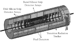
Figure 10: Schematic drawing showing the placements of the Inner Detector Components. A female physicist is shown for size comparison.

The primary functions of the 7.8 metres long and 1.1 metres radius Inner Detector are track reconstruction for charged particles and precise reconstructions of both the interaction vertex (where the hard interaction ocurred) and secondary vertices (where a particle has decayed) in the event. Three distinct subsystems make up the design, all of them with a high tolerance against the tough radiation levels [atlas_inner]: Silicon pixel detectors, Silicon strip detectors (called the SCT: Semi-Conductor Tracking), and Transition Radiation Trackers (TRT). The total cost for these components lies around 400 million DKR, to be compared with the total cost for ATLAS of 2.2 billion DKR.

Particle tracks down to $\approx 9.4^{\circ}$ from the beam pipe can be measured by the Inner Detector system. Often, one sees pseudorapidity used rather than the angle itself:

$$\eta\equiv-\ln\tan(\theta/2)$$ (25)

where $\theta$ is the angle from the beam axis to the radius vector of the point considered. For massless particles, this quantity is equal to the rapidity and transforms additively under Lorentz boosts along the beam direction (by convention, the $z$ direction):

$$\mathcal{L}_{z}(\Delta\eta)\eta=\eta+\Delta\eta$$ (26)

where $\mathcal{L}_{z}$ symbolically expresses a Lorentz boost in the $z$ direction. For hadron colliders, where the CM of the interacting partons is related to the CM of the incoming hadrons by exactly a $z$-boost (neglecting the small transverse momenta of the partons), a quantity with such simple transformation properties is more convenient to work with. In this unit, the beam directions are given by $\eta=\pm\infty$ and the direction transverse to the beam by $\eta=0$. The above statement that particle tracks down to $9.4^{\circ}$ are measured translates to $|\eta|<2.5$. In reality, only particles with transverse momenta, $p_{T}^{2}=p_{x}^{2}+p_{y}^{2}$, above a given threshold can be reconstructed (AtlFast default: $p_{T}>0.5\mbox{\!\ GeV}$). Momenta are measured (SCT and TRT) with an accuracy of approximately $\sigma(p)/p\approx 6\times 10^{-4}p[\mbox{\!\ GeV}]$, and vertex positions (pixels) with radial resolution $\approx 14\mu\mbox{m}$ and longitudinal resolution $\approx 87\mu\mbox{m}$ [atlas_inner].

4.3 Calorimeters

Weighing around 4000 tons, there is ample material in the ATLAS calorimeter system to accomplish its purpose: to completely stop particles and measure the energy they give off as they are decelerated. This is done using arbsorbing materials in which the particles loose energy through collisions interlaced with scintillating media or other signal devices where the particles give off a signal proportional to their energy, enabling energy loss (d$E$/d$x$) and shower profile measurements, highly discriminating variables in particle identification.

4.3.1 EM Calorimeters

Electrons and photons are stopped rather more easily than hadrons, and so the innermost calorimeter in any detector is the Electromagnetic Calorimer. In cylindrical detectors like ATLAS, this is divided into a barrel part and an end-cap part. In ATLAS, the barrel calorimeter, being 6.8​ m long and 4.5​ m in outer diameter, covers $|\eta|<1.475$ i.e. angles larger than $26^{\circ}$ from the beam-pipe while the end-cap region covers $1.375<|\eta|<3.2$ ($\implies 4.5^{\circ}<\theta<28^{\circ}$) [atlas_calo]. Lead and liquid Argon are used as absorber and scintillator, respectively. The individual cells (numbering in the hundred thousands) are constructed in varying sizes (as measured in cartesian coordinates) and are mounted facing the center of the detector such that their $\eta\times\phi$ areas remain constant throughout the subdivisions of the detector with the best resolution ($\Delta\eta\times\Delta\phi=0.025\times 0.025$ corresponding to about 4 by 4 centimetres at $\eta=0$) in the $|\eta|<2.5$ region where also the Inner Detector is active. This high-precision part of the calorimeter can be used to separate e.g. pions, electrons, and photons while the coarser granularity outside means that only measurements of $E_{T}$ and reconstruction of jets is undertaken in that region. The rather crude parametrization of this structure included in AtlFast will be described below.

4.3.2 Hadronic Calorimeters:

The ATLAS hadronic calorimetry consists of three subdetectors: the Hadronic Tile Calorimeter in the central region (barrel and extended barrel, $|\eta|<1.7$), the End-Cap (Liquid Argon) Calorimter in the intermediate region ($1.5<|\eta|<3.2$), and the Forward (Liquid Argon) Calorimeter covering pseudorapidity down to $|\eta|<4.9$ [atlas_calo].

Figure 11: Scematic of a module of the Hadronic Tile Calorimer. The center of the detector lies towards upper right.

The Tile Calorimeter has an outer diameter of 8.5​ m and is about 13​ m long. A division into a barrel ($|\eta|<1$) and two extended barrel parts ($0.8<|\eta|<1.7$) [atlas_tile] with a small gap between is necessary simply because the electronics of the inner parts of ATLAS have to feed out somewhere. Both use steel as the absorbing material, interspersed with scintillating plates. The granularity lies at a planned $\Delta\eta\times\Delta\phi=0.1\times 0.1$, the default for the toy calorimeter used in AtlFast for the central regions of the detector.

Each of the LAr end-caps consists of two copper wheels (2.5 cm and 5cm thickness, respectively) about 2 metres in radius. Up to $|\eta|=2.5$, the granularity is $0.1\times 0.1$ whereafter it becomes $0.2\times 0.2$ up to $|\eta|=3.1$ [atlas_lar]. Lastly, the most challenging of the calorimeters are the Forward Calorimeters. Situated a mere 4.7 metres from the interaction point at high pseudorapidities, the radiation levels here are considerable. The advantages are equally considerable, however, in terms of providing uniform coverage up to $|\eta|=4.9$. For technical reasons, the calorimeter cannot be very long and so must be very dense instead. Three sections, one of copper and two of tungsten, are included in the design [atlas_lar]. As a side remark, Liquid Argon detectors aren’t cheap. All in all, the cost of the Liquid Argon Calorimeters is estimated at slightly less than 600 million DKR, roughly a fourth of the total cost for ATLAS, 2.2 billion DKR [atlas_tp].

4.4 Calorimetry in ATLFAST:

The complex structure described above would be much too cumbersome to fully model in a fast simulation. Instead, AtlFast uses a toy calorimeter where the size of the simulated calorimeter cells in $\eta\times\phi$ coordinates is $0.1\times 0.1$ in the central region ($|\eta|<3$ [atlfast2.0]) and $0.2\times 0.2$ outside (down to $|\eta|=5$). Based on the energy contents of these cells, so-called clusters are searched for – groups of cells close together having larger than nominal energy, i.e. suspected remnants of jets, electrons, or photons. Technically, this is done using the “Snowmass Accord” [stirling96]: Begin by defining a cone of a certain radius in $\eta-\phi$ space, $\Delta R=\sqrt{\Delta^{2}\eta+\Delta^{2}\phi}$ (AtlFast default: $\Delta R=0.4$), sum up the $p_{T}$ inside it, and calculate the position of the $E_{T}$-weighted cluster axis by:

$$E_{T}^{cluster} = \sum_{i\in cone}E_{T}^{i}$$ (27)

$$\phi^{cluster} = \frac{1}{E_{T}^{cluster}}\sum_{i\in cone}E_{T}^{i}\phi^{i}$$ (28)

$$\eta^{cluster} = \frac{2}{E_{T}^{cluster}}\sum_{i\in cone}E_{T}^{i}\eta^{i}$$ (29)

and shift the cone position around until the cone and cluster axes line up. Here, $\phi^{i},\eta^{i}$ is the position of the $i$’th calorimeter cell and we now use $E_{T}$ instead of $p_{T}$ since the calorimeters mesaure energies rather than momenta. This is a slightly pedantic custom since these two quantities are equal for masses that are small compared to the energy, as is the case for hard leptons and jets. The Snowmass definition, however, does not specify how to deal with overlapping clusters, and so a more refined procedure is applied in practice. If two clusters overlap, then merge them into one if there is a lot of $E_{T}$ in the overlap region, else split the energy between if there is only little $E_{T}$.

In AtlFast, only clusters with $E_{T}^{cluster}>10\mbox{\!\ GeV}$ are included in the jet/electron/photon reconstruction. This reconstruction is fairly accurate with errors around 0.04rad [atlfast2.0] for the difference between the initiating parton direction and the center of the reconstructed cluster. The reconstruction of $E_{T}$ is not quite as good, due to energy depositions outside the defined cluster cone. Denoting the difference between the estimated and original parton transverse energies by $\Delta E_{T}=E_{T}^{est.}-E_{T}^{par.}$, a large tail towards negative $\Delta E_{T}/E_{T}^{par.}$ appears with an rms deviation of around 0.2 for the $WH,\ H\to u\bar{u}$ sample process ($m_{H}=100\mbox{\!\ GeV}$) studied in [atlfast2.0]. Since these jets can be loosely categorized as “quark jets from a heavy object”, it is not expected that this error will change greatly for the case of hadronic decays of SUSY particles. It is, however, believed that this error can be corrected for on averrage when the jet energies are recalibrated. In such procedures, one estimates the true parton energy from that estimated by the cone algorithm by [abott01]:

$$E^{par.}=\frac{E^{est.}_{jet}-E_{O}}{R_{jet}S}$$ (30)

where $E_{O}$ is an offset correcting for noise in the detector and energy depositions not associated with the parton jet itself (i.e. the underlying event and pile-up), $R_{jet}$ is a correction for the calorimeter jet energy response and energy lost in cracks, and $S$ is the fraction of energy associated with the jet but not contained within the reconstruction cone. See [abott01] for an excellent and more detailed review of the techniques used in jet energy determinations.

Finally, electrons, photons, and jets are reconstructed from the identified clusters (muons generally leave so little energy in the calorimeters that the cluster criteria are impossible to meet). Electrons, muons, and photons which sit relatively alone in the detector are exceedingly important to measure since they will often be the direct decay products of the hard interaction products. A particle produced in the decay of a fast-moving low-mass particle will generally tend to follow its mother, whereas a particle produced by a high-mass particle which is more or less at rest, will generally sit without much surrounding activity in the detector. Such particles are given the name isolated, and since we shall require all leptons in the analysis to be isolated, we now present the isolation criteria used in AtlFast for electrons and muons.

Electron candidates from the Inner Detector (i.e. with $|\eta|<2.5$) with $P_{T}>5\mbox{\!\ GeV}$ are connected to clusters in the calorimers with a maximum distance between the cluster and the electron of $\Delta R=0.1$. The isolation criteria used as defaults in AtlFast are a separation from any other clusters by at least $\Delta R=0.4$ and an energy deposition of maximally $E_{T}=10\mbox{\!\ GeV}$ in a cone of $\Delta R=0.2$ around the electron. For the sample process $H\to e^{+}e^{-}e^{+}e^{-}$ studied in [atlfast2.0], the efficiency of these criteria was 95.3%, in good agreement with results from full simulation.

For muons, the inner detector is used in combination with the muon system by default. A muon with $|\eta|<2.5$ and $p_{T}>6\mbox{\!\ GeV}$ is a candidate for isolation. By default, the same isolation criteria in terms of energy depositions and cone sizes as for electrons are applied. For the sample process $H\to\mu^{+}\mu^{-}\mu^{+}\mu^{-}$ studied in [atlfast2.0] the efficiency was 97.8% for AtlFast, significantly better than what was obtained by full simulation [atlastdr, table 8-1]: approximately 85% (yielding an efficiency for each muon of roughly $(0.85)^{1/4}=0.96$). In this work, an attempt at obtaining more believable numbers has been made by including by hand estimated electron and muon reconstruction efficiencies. Using the same electron reconstruction efficiency for all energy ranges would be much too crude. Instead, two numbers, depending on the electron $p_{T}$, are used. The assumed electron and muon reconstruction efficiencies, representing educated guesses based on the ATLAS Physics TDR [atlastdr, table 7-1 and table 8-1], are given in table 3.

Particle	Eff($p_{T}<50\mbox{\!\ GeV}$)	Eff($p_{T}>50\mbox{\!\ GeV}$)
Electron	70 %	80 %
Muon	95 %	95 %

Table 3: Assumed reconstruction efficiencies for muons and electrons.

In the end, any clusters which have not been associated with electrons, muons, or photons, are labelled as reconstructed jets if their $E_{T}$ is larger than 15​ GeV. Furthermore, when the detector is running at high luminosity, some pile-up is expected in the calorimeters, i.e. events begin to overlap, worsening the energy resolution. For precision physics, i.e. measurement of the Higgs mass and any exclusive measurements, the degraded resolution can be a serious problem. For the study at hand, note that we wish only to determine if there is and, if so, what type of supersymmetry there is using strictly inclusive quantities, and so a larger smearing of the energy should not significantly affect the result (yet this remains to be verified).

4.5 Muon System

The ATLAS muon spectrometer is composed of three layers of Cathode Strip Chambers (CSC) close to the interaction point and close to the beam axis and Monitored Drift Tube (MDT) chambers over the rest of the coverage (up to $|\eta|=2.7$). The chambers are arranged symmetrically around the beam axis in the barrel region and vertically in the end-cap region. Schematic drawings of the arrangement of the chambers on the sides and on the ends of the detector are shown in figure 12.

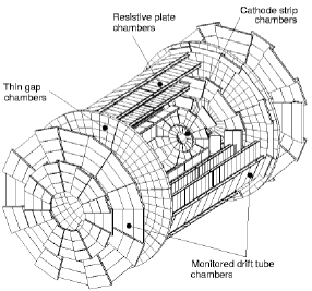
Figure 12: End view and perspective view of the ATLAS muon chambers.

The system is immersed in a magnetic field provided by superconducting air-core toroid magnets with the resulting bending of the muon tracks yielding more precise momentum determinations than could be obtained using the Inner Detector alone. Since one of the main purposes of the muon spectrometer is to enable a mass measurement for very narrow Higgs signals, it is quite important that a mass resolution of about 1% can be obtained this way. The foreseen resolution, as given in the Technical Design Report for the Muon Spectrometer lies at $\Delta p_{T}/p_{T}\approx 2\%$ for muons of $p_{T}$ between 20 and 100​ GeV. For 1000 ​ GeVmuons, this resolution worsens by a factor of roughly 5 [atlas_muon].

In addition to the performance at high $p_{T}$, low-$p_{T}$ muons from $B$ decays require a system containing as little “dead” material as possible. This is among the main reasons that an air core design for the magnets was chosen, resulting in muons down to 3​ GeVsurviving to be measured by the muon system, the hadron calorimeter being the largest absorber on the way.

Also included in the muon spectrometer is a muon trigger system, extending to $|\eta|<2.4$, increasing the precision of the muon trigger and the identification of which of the pulsed beam segments, or “bunches”, of the LHC (spaced by 25ns [atlastdr]) the event belonged to. In addition, the trigger information, though less precise, can be used to supplement the measurements made in the precision chambers with an extra coordinate.

5 Analysis of ATLAS $L$/ -SUSY Discovery Potential

There is at present no experimental evidence either for or against supersymmetry in nature, although some significant exclusion limits have been acheived at LEP. This picture is expected to change drastically over the next few decades, hopefully already within the next ten years. It has been argued above that supersymmetry can only solve the hierarchy problem if the sparticle masses are not significantly larger than the ​ TeV scale. This range is within reach of second generation hadron machines such as the LHC, and so we expect to see direct production and decay of supersymmetric particles relatively soon if supersymmetry exists. On the other hand, the non-observation of supersymmetric processes will disfavour low-energy supersymmetry almost to the point of exclusion, giving us a powerful clue that we must look to some alternate mechanism for solving the hierarchy problem. Whatever the case, it is not unreasonable to suppose that the resolution of the hierarchy problem will give some observable effects at the ​ TeV scale, and so we find ourselves almost guaranteed that interesting experimental results will be obtained in the not too distant future. This section deals with the possible observable consequences of lepton number violating supersymmetry at the ATLAS detector, one of four detectors being built for the LHC and scheduled to go online in 2006.

The organization of the section is as follows: In 5.1, we define the points in mSUGRA space and the scenarios for the $L$-violating couplings we will be using in the analysis. Next, in 5.2 we propose trigger menus dedicated to searches for $L$/ -SUSY at mid-luminosity running of the LHC ($L=3\times 10\times 10^{33}\mbox{\!\ cm${}^{-2}$s${}^{-1}$}$). At this luminosity, pile-up is expected, meaning that several events are recorded simultaneously by the detector, degrading the energy resolution. Since there are no tools presently available to parametrize this for mid-luminosity running, we account for this effect in a very crude manner by simply scaling the simulated event rates by a common factor.

In 5.3 and 5.4, the main part of the analysis is presented, concentrating on what can be achieved with an amount of data corresponding to an integrated luminosity of 30​ fb^-1. It is divided into two parts, one based on cuts and one based on neural networks. The purpose of the first part is to choose cuts on several kinematical and inclusive variables which isolate a fairly broad event sample enriched in supersymmetric events with no emphasis on any particular scenario, except of course that lepton number is assumed violated. The purpose of the second part is to process this event sample with neural networks trained to recognize particular scenarios. Due to the large luminosity at the LHC, it has not been possible to generate an event sample of comparable magnitude to 30​ fb^-1 of data taking for the highest cross section backgrounds. For $Z/W$ production and moderate $p_{T}$ QCD processes, each generated event thus corresponds to hundreds of events expected in data. For these event samples, the large rejection factors reached will eventually cause only a very few or zero events to remain after cuts. At this point, we estimate the event numbers by 95% confidence upper limits, fitting to the event distribution below the cut or by using Poisson statistics on the number remaining after the cut (see [europhys, feldman98]). Rejection factors for these events are in principle unknown but can be pessimistically estimated using the rejection factors for the high $p_{T}$ QCD sample and the double gauge events. Lastly, in 5.5 the results of the cut-based analysis combined with the nerual network classification are presented.

5.1 Points of Analysis

	$\mathbf{P_{2}}$	$\mathbf{P_{7}}$	$\mathbf{P_{9}}$	$\mathbf{P_{12}}$	$\mathbf{F_{2}}$
GUT Parameters
$\tan\beta$	5	10	20	35	10
$m_{0}$	170	335	100	1000	2100
$m_{\frac{1}{2}}$	780	1300	300	700	600
sign$(\mu)$	+	+	+	$-$	+
$A_{0}$	0	0	0	0	0
Mass Spectrum
$h^{0}$	118	123	115	120	119
$A^{0},H^{\pm},H^{0}$	110	1663	416	944	2125
$\tilde{\chi}^{0}_{1}$	325	554	118	293	239
$\tilde{\chi}^{0}_{2},\tilde{\chi}^{+}_{1}$	604	1025	217	543	331
$\tilde{\chi}^{0}_{3}$	947	1416	399	754	348
$\tilde{\chi}^{0}_{4},\tilde{\chi}^{+}_{2}$	960	1425	416	767	502
$\tilde{g}$	1706	2752	707	1592	1442
$\tilde{e}_{R},\tilde{\mu}_{R}$	336	584	156	1031	2108
$\tilde{\tau}_{1}$	334	574	126	916	2090
$\tilde{e}_{L},\tilde{\mu}_{L}$	546	917	231	1098	2126
$\tilde{\tau}_{2}$	546	915	240	1051	2118
$\tilde{\nu}$	541	913	217	1095	2125
$\tilde{q}_{R}$	1453	2333	612	1612	2328
$\tilde{b}_{1}$	1403	2262	566	1412	2010
$\tilde{t}_{1}$	1189	1948	471	1241	1592
$\tilde{q}_{L}$	1514	2425	633	1663	2343
$\tilde{b}_{2}$	1445	2312	615	1482	2310
$\tilde{t}_{2}$	1443	2286	648	1451	2018

Table 4: Selected points of analysis in the mSUGRA parameter space.

	$a$	$b$	$n$
LLE : Purely Leptonic Lepton Number Violation
$\begin{array}[]{c}\lambda_{ijk}\\ \lambda^{\prime}_{ijk}\end{array}$	$\begin{array}[]{c}10^{-2}\\ 0\end{array}$	$\begin{array}[]{c}10^{-4}\\ 0\end{array}$	$\begin{array}[]{c}\sqrt{\hat{m}_{e_{i}}\hat{m}_{e_{j}}\hat{m}_{e_{k}}}\\ 0\end{array}$
LQD : Minimally Leptonic Lepton Number Violation
$\begin{array}[]{c}\lambda_{ijk}\\ \lambda^{\prime}_{ijk}\end{array}$	$\begin{array}[]{c}0\\ 10^{-2}\end{array}$	$\begin{array}[]{c}0\\ 10^{-4}\end{array}$	$\begin{array}[]{c}0\\ \sqrt{\hat{m}_{e_{i}}\hat{m}_{q_{j}}\hat{m}_{d_{k}}}\end{array}$
LLE + LQD : Mixed Lepton Number Violation
$\begin{array}[]{c}\lambda_{ijk}\\ \lambda^{\prime}_{ijk}\end{array}$	$\begin{array}[]{c}10^{-2}\\ 10^{-2}\end{array}$	$\begin{array}[]{c}10^{-4}\\ 10^{-4}\end{array}$	$\begin{array}[]{c}\sqrt{\hat{m}_{e_{i}}\hat{m}_{e_{j}}\hat{m}_{e_{k}}}\\ \sqrt{\hat{m}_{e_{i}}\hat{m}_{q_{j}}\hat{m}_{d_{k}}}\end{array}$

Table 5: Selected points of analysis in the $\lambda-\lambda^{\prime}$ parameter space. The models with natural couplings (coloumn $n$) will be referred to as “nLLE”, “nLQD”, and “nLLE + nLQD” in following sections. If the couplings get significantly smaller than $10^{-4}$, the LSP lifetime can become so large that it decays outside the detector, mimicking the $R$-conserving scenarios. For example, for the mSUGRA point $F_{2}$, setting all $\lambda$ couplings to $10^{-6}$ and all $\lambda^{\prime}$ couplings to zero results in a decay length for the LSP of $\tau c=40\mbox{m}$. In the intermediate range, one may see the effects of neutralino decay either as a secondary vertex or as a decay inside the fiducial volume of the detector. Naturally, such spectacular signatures would greatly lessen the effort required to discover SUSY, yet we abstain from studying such scenarios here so as not to be overly optimistic in our results.

For reasons of simplicity, we concentrate on a few points in the mSUGRA parameter space. These points have not been chosen among the ones initially suggested in the ATLAS Physics TDR. This is partly due to the exclusion of all these points by LEP (essentially from bounds on the Higgs mass), and partly since it is interesting to enable a direct comparison between the capabilities of the LHC and other, future experiments such as CLIC (Compact LInear Collider), a 3​ TeV electron-positron collider currently under study at CERN. On these grounds, the analysis is performed on a selection of points defined by the CLIC physics study group. A general drawback to any selection of points defined within the MSSM framework is of course that they are constructed to make the lightest neutralino the LSP. In an $R$-Violating scenario, this condition does not apply, and so one should bear in mind that the full parameter space can never be analyzed using just MSSM points, though an attempt at defining new points for $R$-Violating scenarios would go beyond the scope of this work. The 5 mSUGRA points shown in table 4 have been selected among 14 points defined by the CLIC physics study group on the basis that they represent the broadest possible range within those points. Let it be emphasized that I am not aiming to do precision physics in this work, but rather to estimate the sensitivity for $L$/ -SUSY for various mass hierarchies. It is therefore not interesting whether we are sensitive to one or another particle or which exact numerical values the masses have. What is interesting is how sensitive we are for light/medium/heavy masses for the lightest neutralino in particular and for various possibilities for the other masses. In this light, there is a great redundancy in the 14 CLIC points, and thus the 5 points given in table 4 have been chosen for their mutual differences.

In addition, values for the $R$-Violating couplings must be specified. The experimental upper bounds lie around $10^{-1}-10^{-2}$ for most couplings [rvbounds], depending on the masses of the squarks and sleptons, with heavier masses allowing larger couplings. For the cases of purely leptonic (LLE), mixed (LLE+LQD), and minimally leptonic (LQD) Lepton number violation, three models are investigated beyond the MSSM without modification. Firstly, two points with common values for all couplings, and secondly a model with generation-hierarchical couplings defined by [hinchliffe93]:

$$\begin{array}[]{rcl}|\lambda_{ijk}|^{2}&=&\hat{m}_{e_{i}}\hat{m}_{e_{j}}\hat{m}_{e_{k}}\\ |\lambda^{\prime}_{ijk}|^{2}&=&\hat{m}_{e_{i}}\hat{m}_{q_{j}}\hat{m}_{d_{k}}\end{array}\hskip 28.45274pt;\hskip 19.91684pt\hat{m}\equiv\frac{m}{v}=\frac{m}{126\mbox{\!\ GeV}}$$ (31)

where $m_{q_{j}}$ represents the mass of “a quark of generation $j$”. Due to the mass splittings of the quarks, this definition is inherently ambiguous. A way to resolve the ambiguity suggested by [hinchliffe_private] is to set $m_{j}$ equal to the arithmetic mean of $m_{u_{j}}$ and $m_{d_{j}}$ where $u$ and $d$ stand for up-type and down-type respectively:

$$m_{q_{j}}={\textstyle\frac{1}{2}}(m_{u_{j}}+m_{d_{j}})$$ (32)

This procedure is the one implemented in PYTHIA. The resulting coupling scenarios are given in table 5.

An additional noteworthy remark is that while small $R$/  couplings have little or no impact on the masses and couplings at the electroweak scale, large $R$/  couplings (as compared to the other couplings in the theory) can have significant effects through loops when evolving the Renormalization Group Equations (RGE’s) from the input scale to the ​ TeV scale. This is currently not included in PYTHIA. The $R$/  couplings are simply switched on at the low scale and the interplay between the $R$/  couplings and other physics is neglected. Order-of-magnitude-wise, this assumption breaks down for $\lambda^{(^{\prime})}>10^{-2}$, and so some effort should be devoted to including the full RGE’s in simulations of $R$/ -SUSY. Also, the CLIC points assume a vanisgin trilinear coupling at the GUT scale, i.e. $A_{0}=0$. In connection with this work, a small study of the direct consequences of that assumption upon the results presented here was performed (see section LABEL:sec:assumptions) with the conclusion that the semi-inclusive branching ratios (e.g. $BR(\tilde{\chi}^{0}_{1}\to qq\nu)$) depend only very weakly on this parameter ($\mathcal{O}(5\%)$), and so the main signatures (number of leptons, number of jets, etc.) should be only mildly affected by changes to this parameter.

5.2 Trigger Selection

The cross sections for SUSY production at the LHC for the points studied in this work range from $10^{-8}$–$10^{-12}$mb. For comparison, the cross section for e.g. $Z/W$ production is $10^{-3}$mb, and the total interaction cross section (excepting elastic and diffractive processes which do not give rise to hard jets, leptons, or neutrinos) is around 70mb, mostly consisting of small-angle QCD interactions. Background rejection is thus extremely essential. In an ideal world, all data recorded by the experiment would be written to disk for later scrutiny. With the extreme event rates and sizes (approximately 1 billion events per second and approximately 1MB per event[atlastdr]) at the LHC, such a strategy is entirely out of the question, moreover it is completely uncalled for. The extreme rates are only necessary to enable us to reach the very small Higgs and New Physics production cross sections. As already mentioned, the vast majority of events are QCD processes with small momentum transfers. Relative to how much statistics we need to study those processes, we get a huge over-abundance. We can then accept to limit the data flow by cutting away a significant fraction of those events and writing only a very small subset of them to disk, along with events which contain possible traces of low cross section physics. To accomplish this reduction, an extensive trigger system is being developed for ATLAS which will identify the (possibly) interesting events and reject uninteresting ones. For SUSY, typical signatures that can be triggered on include a lot of missing transverse energy ($E_{T}/\hskip 6.49994pt$) and large (hard) jet and lepton multiplicities. The usefulness of the “classical” SUSY $E_{T}/\hskip 6.49994pt$ signature will in general be decreased in $R$/  scenarios due to LSP decay, but it remains of some discriminating power. On the other hand, the LSP decays to jets, leptons, and/or neutrinos, and so the signature is merely transformed, not lost. We can use this to define a set of triggers that will reject the QCD background (which typically has small $E_{T}/\hskip 6.49994pt$ and jet/lepton multiplicities) but keep the majority of those events that might have been caused by the production and decay of supersymmetric particles.

5.2.1 $L$/ -SUSY Triggers at Mid-Luminosity

The acceptable rate of events that can be written to disk is about 100Hz. The sum rate of all the triggers which will be implemented in ATLAS must therefore stay below this number. This includes triggers for Higgs physics, $B$ physics, $Z/W$ physics, and all kinds of New Physics triggers, of which $R$/ -SUSY is only one. A reasonable aim for the trigger rate for the $R$/ -SUSY triggers is therefore about 1Hz. Since no detailed trigger rate studies for mid-luminosity running are yet available, I here present some crude estimates for the trigger rates for various trigger possibilities. It should be understood that there are quite significant uncertainties associated with these, as one might well imagine when already uncertain quantities are extrapolated over orders of magnitudes in their domain. The jet rates, especially, are not well under control, although interesting work is in progress [webber00, forshaw99, seymour00]. It has not been possible here to perform a systematic study of the effects of varying QCD parameters on the trigger rates, yet it is useful in the following to keep in mind that the multi-jet rates can be uncertain by factors of 2 or more [atlfast2.0].

The only processes which have rates above the 1Hz domain are QCD $2\to 2$ processes and $Z/W$ production, the former with a cross section around 70mb (but strongly peaked distributions), the latter with a cross section around $10^{-3}$mb with more broad distributions and so more likely to be triggered on (By “$Z/W$” production is meant the sum of $Z$, including photon interference, and $W$ production). In this crude study, we shall not focus on where in the trigger system which triggers are placed (i.e. LVL1, LVL2, or LVL3). This is a technical issue which requires more detailed knowledge of the detector performance at mid-luminosity than is currently available in AtlFast. Specifically, running at mid- and high luminosity means that there can be several interactions recorded simultaneously by the detector (pile-up), leading to some smearing of event distributions. Since the whole point is that most events should lie outside the trigger domain than inside it, more events will be smeared into the trigger domain than out of it, increasing the trigger rates when pile-up is at play. This is currently only parametrized in AtlFast for high luminosity. We here adopt a crude buest-guess approach, performing the simulation for low luminosity, i.e. without pile-up, and multiplying the resulting trigger rates by 5 instead of 3 to get from $L=10^{33}\mbox{\!\ cm${}^{-2}$s${}^{-1}$}$ to $L=3\times 10^{33}\mbox{\!\ cm${}^{-2}$s${}^{-1}$}$. This number is based on the scaling exhibited by the trigger rates presented in [atlastdr, chp.11] from $L=10^{33}\mbox{\!\ cm${}^{-2}$s${}^{-1}$}$ to $L=10^{34}\mbox{\!\ cm${}^{-2}$s${}^{-1}$}$ where factors between 1 and 5 are found between triggers at equal thresholds after dividing out the factor 10 caused by the luminosity difference. The triggers for which this direct comparison was possible were the inclusive electron, electron/photon, and $E_{T}/\hskip 6.49994pt$+2jets triggers. Since we are here interested in going from $L=10^{33}\mbox{\!\ cm${}^{-2}$s${}^{-1}$}$ to $L=3\times 10^{33}\mbox{\!\ cm${}^{-2}$s${}^{-1}$}$, a factor of 5/3 was deemed suitable. These rates should then to be understood as corresponding to LVL3 trigger rates. Suitable intermediate trigger levels will presumably be studied in more detail and with full detector simulation by the ATLAS trigger/DAQ community in the near future.

Returning to the issue at hand, we now propose 11 trigger menus for SUSY searches in $L$/  scenarios (bearing in mind the many possible signatures in these scenarios). Granting that the LSP might be the neutralino even in $L$/  scenarios, it is tempting to define triggers based on the neutralino decay channels, $qq\nu$, $qq\ell$, and $\ell\ell\nu$. This would work well at all of the SUSY points analyzed here since all of them have a neutralino LSP, but one should keep in mind that the lightest neutralino need not be the LSP when $R$ is violated. Let us therefore go back to the terms in the superpotential that we are after: $LLE$ and $LQD$, i.e. a coupling between three (s)leptons and a coupling between two (s)quarks and one (s)lepton, where only one of the particles coupling in each case will be a sparticle. From this very general standpoint, obvious trigger strategies suggest themselves.

In the case of the first coupling (LLE), we are searching for a number of leptons (depending on whether one or two supersymmetric particles were produced and whether they decayed into two- or three-body channels), possibly accompanied by $E_{T}/\hskip 6.49994pt$. We do not here consider an all-neutrino signature since this would be equivalent to the $R$-conserving SUSY $E_{T}/\hskip 6.49994pt$ signature. We require: at least two isolated electrons and/or muons or one isolated $e$ or $\mu$ accompanied by $E_{T}/\hskip 6.49994pt$.

For the $LQD$ term, we expect jets accompanied by leptons or $E_{T}/\hskip 6.49994pt$. The triggers proposed are: at least 3 jets accompanied by either $E_{T}/\hskip 6.49994pt$ or at least one isolated $\mu$ or $e$, or at least 1 jet, accompanied by the same with higher thresholds. Each trigger was studied for several possibilities and combinations of trigger thresholds. The complete scans around the selected threshold values are shown and commented in Appendix LABEL:app:trigger.

Trigger	Background Rate	MSSM Efficiency	LLE Efficiency	LQD Efficiency
mu45I + mu45I	0.2 Hz	1 — 5 %	10 — 40 %	1 — 10 %
e45I + e45I	0.1 Hz	1 — 5 %	1 — 35 %	1 — 10 %
mu15I + e15I	0.1 Hz	2 — 5 %	20 — 60 %	2 — 15 %
mu40I + me75	0.3 Hz	10 — 25 %	40 — 75 %	10 — 35 %
e40I + me75	0.2 Hz	10 — 20 %	15 — 70 %	10 — 35 %
j100 + mu40I	0.5 Hz	10 — 20 %	45 — 70 %	10 — 40 %
j100 + e40I	0.5 Hz	5 — 15 %	15 — 65 %	10 — 35 %
j100 + me175	0.3 Hz	50 — 80 %	35 — 80 %	25 — 80 %
3j50 + mu20I	0.1 Hz	5 — 15 %	45 — 60 %	12 — 40 %
3j50 + e30I	0.1 Hz	5 — 10 %	15 — 55 %	10 — 35 %
3j75 + me125	0.1 Hz	30 — 65 %	30 — 70 %	40 — 90 %
Total Rate /Combined Efficiency	2.1 Hz	60 — 90 %	90 — 99.9 %	60 — 96 %

Table 6: Estimated trigger rates for background processes and trigger efficiency ranges for the various MSSM points and $L$/ -SUSY scenarios studied for $L=3\times 10^{33}\mathrm{cm}^{-2}\mathrm{s}^{-1}$ (summary of plots in appendix LABEL:app:trigger). The trigger symbols are described in the text. The total trigger rate is slightly smaller than the sum of the individual rates, since one event can fulfil several trigger criteria. One sees how much cleaner the signatures of the purely leptonic (LLE) coupling are compared to the signatures involving quarks (LQD) where higher thresholds, due to the hadronic environment, mean smaller efficiencies.

Here, event rates for the selected values of the trigger cuts are given in table 6 where also the efficiencies with which these triggers allow signal events to pass are listed. The nomenclature for each trigger item is such that e.g. ‘mu20I’ and ‘e40I’ mean ‘a muon with $p_{T}>20\mbox{\!\ GeV}$ which is isolated’, and ‘an isolated electron with $p_{T}>40\mbox{\!\ GeV}$’, respectively. ‘3j100’ and ‘me80’ mean three reconstructed jets of (each) more than 100​ GeV $p_{T}$ and more than 80​ GeVmissing transverse energy, respectively. To save space, the signal trigger efficiencies are given as ranges (min—max), obtained by dividing the scenarios studied into three categories and scanning for the minimum and maximum efficiencies within each category. These categories are: the MSSM (for reference), purely leptonic $L$/  (i.e. decays proceeding via the $\lambda$ couplings (LLE)), and mixed quark-lepton $L$-violation (the $\lambda^{\prime}$ couplings (LQD)). Scenarios where both types of couplings are non-zero generally lie inbetween the two extremes, depending on the relative coupling strengths. The efficiency ranges reached by combining all the triggers are shown in the bottom of the table.

5.2.2 Final Remarks

Though these trigger proposals are designed explicitly with $R$/ -SUSY in mind, they show a certain overlap with triggers proposed for more conventional physics. The di-muon and 3 jets + lepton triggers, for example, have also been proposed for various Higgs searches. The di-electron trigger as well as 3 jets + electron are proposed to catch $t\bar{t}$ decays. Finally, the conventional SUSY searches also make use of multi-lepton, jets + $E_{T}/\hskip 6.49994pt$, and multi-jet signatures [bystricky96]. It is therefore not unthinkable that the triggers here proposed can be incorporated to some extent into the conventional trigger programme, possibly enabling a relaxation of the trigger thresholds for the remaining objects.

Finally, though no study of the mutual redundancy among these trigger objects has been performed, one sees from table 6 that e.g. the di-electron trigger and the 3-jet + electron trigger have low efficiencies, this mainly due to the low electron reconstruction efficiency which is required to be sure one is not mistakenly believing a jet to be an electron (see [atlastdr, table 7-1] for estimated jet rejection factor as function of electron reconstruction efficiency). As a suggestion for future analyses, it might be worthwile to investigate what happens if one dispenses with these two triggers, replacing them with e.g. two-jet + leptons or two-jet + $E_{T}/\hskip 6.49994pt$ triggers instead, yet caution in such undertakings is advisable. The presence of electron triggers is, for example, essential in catching scenarios where the first generation $L$/  couplings are dominant. This is the reason why as little dependence on lepton flavour as possible has been strived for in the menus here proposed.

5.3 Discriminating Variables

We now come to the cut-based analysis. The purpose here is to define a set of discriminating variables, i.e. variables capable of distinguishing in a statistical sense between the SM and the various SUSY scenarios. Once defined, the idea is to use these variables and our knowledge of their distributions in SM and non-SM scenarios to isolate a sample of events with maximal possible enrichment of SUSY events and minimally contaminated by SM events. At this point, we do not seek to distinguish between or aim the analysis towards any particular SUSY scenarios, except that we assume the LSP to decay through violation of lepton number.

In the following pages, a number of kinematical and inclusive variables are presented. The distributions of each variable in the SM and in the mSUGRA models determine at which values of the variables cuts should be placed. In a conventional analysis of this type, one would seek to maximize the statistical significance with which a signal can be extracted by adapting the analysis to maximize quantities like $S/B$, $S/(S+B)$, or $S/\sqrt{S+B}$, where $S$ and $B$ are the number of signal events and the number of background events, respectively, remaining after the analysis. Obviously, this requires knowledge about the shapes of both signal and background distributions in each of the discriminating variables. In the present case, we wish to study a class of models rather than individual models, and so no unique shape can be assigned to the signal we are looking for, other than general qualities such as, for example, an excess of leptons in the purely leptonic $L$/ -SUSY scenarios. We are therefore not in a position to optimize the analysis with respect to exactly quantifiable estimators. Of course, an analysis could be performed and optimized point by point, yet such a strategy would have to be carried out on a more general set of mSUGRA points, so as not to over-tune the analysis to exactly the points considered, risking to loose sensitivity to points not studied. Moreover, more is perhaps learned by generalizing and looking for common discriminators than spending a large effort studying closely hundreds of scenarios which may have nothing to do with what the experiment finds. This is the real motivation why the last part of the analysis is done using neural networks. They serve to approximate dedicated search strategies for specific scenarios.

Let us begin by considering which backgrounds are most important. Firstly, QCD $2\to 2$ processes and $Z/W$ production have the highest cross sections. As before, we mean by $Z/W$ the sum of $Z$ and $W$ production. Secondly, one must expect that the more mass there is in an SM event, the more dangerous it is when trying to look for heavy physics. $t\bar{t}$ production, $ZZ/ZW/WW$ production, and Higgs production are examples of heavy SM backgrounds. Again, by $ZZ/ZW/WW$ production is meant the sum of $ZZ$, $ZW$, and $WW$ production. The Higgs is not expected to be extremely dangerous, since its mass will presumably be known before LHC SUSY searches begin, and since the cross sections are low (e.g. $\sigma(Z/W+h^{0})=2.5\times 10^{-9}\mbox{\!\ mb}$ for $m_{H}=115\mbox{\!\ GeV}$). With respect to the large lepton and jet multiplicity as well as large $E_{T}/\hskip 6.49994pt$, one could well ask how significant triple gauge production could be as background. Unfortunately, these production cross sections are not yet implemented in PYTHIA, and so we are forced to give a rough estimate based on the $\alpha_{EW}^{2}$ suppression, i.e. a factor $10^{-4}$ relative to $ZZ/ZW/WW$ production. This brings the cross section down to about $10^{-11}$mb. Special cuts designed to catch pairs of jets or leptons with $Z$ or $W$ invariant masses and requiring that the $p_{T}$ of a jet or a lepton be larger than $\approx$50 ​ GeV (see below) would most likely bring this contamination down by at least a factor ten more. Furthermore, we shall see that even the double gauge events give a neglegible contribution to the background at the end of the analysis, and so I conclude it safe to disregard this background when the SUSY cross section is larger than $10^{-12}\mbox{\!\ mb}$. For lower cross sections than this, it would be advisable to conduct a dedicated study of how the triple gauge background can be dealt with, but in such regions, the total number of SUSY processes recorded by the ATLAS detector will also be so small that the LHC is at the limit of its capabilities (see point 7 in the table below), and so for such studies to be meaningful, full detector simulation as well as much more dedicated (i.e. specialized) search strategies are necessary.

SM Process	$\sigma$ [mb]	$N_{\mathrm{gen}}$	$N_{\mathrm{trig}}$	$N(30\mbox{\!\ fb}^{-1})$	$N_{\mathrm{trig}}(30\mbox{\!\ fb}^{-1})$
QCD $2\to 2$
$p_{T}<100\mbox{\!\ GeV}$	70	—	—	2$\times 10^{15}$	$<10^{5}$
$p_{T}=100-150\mbox{\!\ GeV}$	1.42$\times 10^{-3}$	1.0$\times 10^{8}$	320	4.26$\times 10^{10}$	$(1.4\pm 0.1)$$\times 10^{5}$
$p_{T}>150\mbox{\!\ GeV}$	2.88$\times 10^{-4}$	3.1$\times 10^{7}$	5.6$\times 10^{3}$	8.64$\times 10^{9}$	1.7$\times 10^{6}$
$Z/W$	1.19$\times 10^{-3}$	1.8$\times 10^{8}$	4.1$\times 10^{4}$	3.57$\times 10^{10}$	8.1$\times 10^{6}$
$t\bar{t}$	6.08$\times 10^{-7}$	5.9$\times 10^{6}$	8.1$\times 10^{5}$	1.82$\times 10^{7}$	2.6$\times 10^{6}$
$ZZ/ZW/WW$	1.16$\times 10^{-7}$	5.9$\times 10^{6}$	1.5$\times 10^{5}$	3.48$\times 10^{6}$	8.9$\times 10^{4}$

Table 7: Cross sections and event numbers for SM processes. $N_{\mathrm{gen}}$ is the total number of generated events, and $N_{\mathrm{trig}}$ is the number passing trigger thresholds. The fourth column simply contains the cross section multiplied by $30\mbox{\!\ fb}^{-1}$ and the last is the number of generated events passing trigger thresholds scaled to 30$\mbox{\!\ fb}^{-1}$ of data taking: $N_{\mathrm{trig}}(30\mbox{\!\ fb}^{-1})=N_{\mathrm{trig}}\times N(30\mbox{\!\ fb}^{-1})/N_{\mathrm{gen}}$. For the lowest $p_{T}$ QCD sample, none of the generated events passed triggers. The estimate of less than $10^{5}$ events is discussed in the text. For the intermediate $p_{T}$ QCD sample, the number of generated events passing triggers was so low that the associated statistical uncertainty is shown with the scaled number. No correction for pile-up is included in these numbers.

mSUGRA Point	$\sigma$ [mb]	$N_{\mathrm{gen}}$	$N_{\mathrm{trig}}$	$N(30\mbox{\!\ fb}^{-1})$	$N_{\mathrm{trig}}(30\mbox{\!\ fb}^{-1})$
$P_{2}$	1.3$\times 10^{-10}$			3900
MSSM		$10^{5}$	8.9$\times 10^{4}$		3500
LLE		$10^{5}$	9.9$\times 10^{4}$		3900
nLLE		$10^{5}$	9.8$\times 10^{4}$		3800
LQD		$10^{5}$	9.4$\times 10^{4}$		3700
nLQD		$10^{5}$	9.4$\times 10^{4}$		3700
$P_{7}$	3.9$\times 10^{-12}$			114
MSSM		$10^{5}$	8.2$\times 10^{4}$		94
LLE		$10^{5}$	9.9$\times 10^{4}$		113
nLLE		$10^{5}$	9.9$\times 10^{4}$		113
LQD		$10^{5}$	9.8$\times 10^{4}$		111
nLQD		$10^{5}$	9.7$\times 10^{4}$		111
$P_{9}$	2.4$\times 10^{-8}$			720000
MSSM		8.2$\times 10^{5}$	6.7$\times 10^{5}$		590000
LLE		8.4$\times 10^{5}$	8.0$\times 10^{5}$		690000
nLLE		8.2$\times 10^{5}$	7.3$\times 10^{5}$		640000
LQD		8.4$\times 10^{5}$	5.9$\times 10^{5}$		510000
nLQD		8.4$\times 10^{5}$	5.7$\times 10^{5}$		490000
$P_{12}$	1.1$\times 10^{-10}$			3300
MSSM		$10^{5}$	8.8$\times 10^{4}$		2900
LLE		$10^{5}$	9.9$\times 10^{4}$		3300
nLLE		$10^{5}$	9.7$\times 10^{4}$		3200
LQD		$10^{5}$	8.8$\times 10^{4}$		2900
nLQD		$10^{5}$	8.6$\times 10^{4}$		2800
$F_{2}$	1.1$\times 10^{-10}$			3300
MSSM		$10^{5}$	6.1$\times 10^{4}$		2000
LLE		$10^{5}$	9.7$\times 10^{4}$		3200
nLLE		$10^{5}$	8.8$\times 10^{4}$		2900
LQD		$10^{5}$	7.1$\times 10^{4}$		2300
nLQD		$10^{5}$	6.0$\times 10^{4}$		2000

Table 8: Cross sections and event numbers for mSUGRA. Since single sparticle production is not included, the choice of a scenario with or without $L$/  does not affect the production cross sections. The LLE/LQD models correspond to the models in column $a$ of table 5 and the nLLE/nLQD to column $c$. The models in column $b$ are generally so similar to the ones in column $a$ that they have been left out of this table. The same goes for the LLE+LQD models which simply interpolate between the LLE and LQD scenarios. No correction for pile-up is included in these numbers.

The numbers of events used in the analysis are shown in tables 7 and 8 together with cross sections, the number of generated events passing trigger thresholds, and the number of events expected after an integrated luminosity of 30​ fb^-1 has been collected. As can be seen, the number of events expected for $P_{7}$ is only around 100. This is most likely too low for ATLAS to see anything, yet the mass hierarchy in the model is interesting, and so we include it in the analysis to give an exampel of the performance of this type of model under the tested cuts.

QCD processes with the $p_{T}$ of the hard interaction in its rest frame below 100​ GeV were not possible to include in the analysis, since none of the events generated for the trigger studies passed the selected trigger thresholds. Though the statistical uncertainty on 0 events clearly does not make sense to define, a conservative estimate on the maximal number of events passing triggers can be obtained by noting that a Poisson distribution with mean $\mu=2.99$ has less than 5% probability of resulting in 0 events, and so we estimate the event numbers by scaling 3 events out of each of the generated $p_{T}<100\mbox{\!\ GeV}$ samples to $30\mbox{\!\ fb}^{-1}$ of data taking. This brings us to conclude that at most 1.9$\times 10^{7}$ events in the region $1\mbox{\!\ GeV}<p_{T}<10\mbox{\!\ GeV}$, 5.0$\times 10^{6}$ events in the region $10\mbox{\!\ GeV}<p_{T}<75\mbox{\!\ GeV}$, and at most 4.9$\times 10^{4}$ events in the region $75\mbox{\!\ GeV}<p_{T}<100\mbox{\!\ GeV}$ could pass trigger thresholds with a 5% chance that we would not have seen them in the trigger analysis. Though these numbers are statistically sound, the estimates for the two lowest $p_{T}$ samples are likely to be gross overestimates. That particles from the first class of events should be able to gain enough $p_{T}$ through parton showering, hadronization, and detector resolution alone to pass any of the triggers here used borders on the impossible. With respect to events from the second class ($10-75\mbox{\!\ GeV}$), we note that the $E_{T}/\hskip 6.49994pt$ triggers used begin at 75​ GeV with the further requirement of hard, isolated leptons and that the jet triggers require either 3 jets of each 50​ GeV $p_{T}$ or 1 jet with $p_{T}=100\mbox{\!\ GeV}$, and so it is also here excessively unlikely to see events passing into the active trigger range. Towards the high end of the $p_{T}$ region, though, and for the third class of events, there are clearly some events in the far extremes of the distributions which will pass trigger thresholds. Estimating the upper bound on this number to be ten times that estimated for the third class of events alone seems the best guess possible at the moment, and so we arrive at an estimated maximum of $10^{6}$ $p_{T}<100\mbox{\!\ GeV}$ QCD events which are not included in the analysis. Assuming, pessimistically, that these events will have the same rejection factors under the cuts applied below as the $p_{T}=100-150\mbox{\!\ GeV}$ QCD sample, we will see that an additional $10^{6}$ low-$p_{T}$ QCD events will not significantly affect the conclusions of the analysis.

No attempt at including the effects of pile-up has been implemented in the analysis. Generally speaking, pile-up results in smearing of the measured calorimeter energies. Acknowledging that this would shift more events into the active trigger range than out of it, we made a guess at an overall factor of 5/3 for the trigger study, i.e. the rates obtained for $L=3\times 10^{33}\mbox{\!\ cm${}^{-2}$s${}^{-1}$}$ without smearing were multiplied by this number to obtain a more realistic estimate. This was done noting that:

$$R(thres)\propto\int_{thres}^{\infty}\!\!\mbox{d}p_{T}\!\ \phi_{smeared}(p_{T})=C(thres)\int_{thres}^{\infty}\!\!\mbox{d}p_{T}\!\ \phi(p_{T})$$ (33)

i.e. the rate passing a certain threshold is proportional to the integral from that threshold to infinity of the smeared distribution of events, which can be written as a (threshold-dependent) constant times the integral of the unsmeared distribution, or in simpler words: a number can always be written as a constant times another number. In the last section, we assumed $C(thres)=5/3$. In the analysis, however, we are looking at the distributions themselves rather than their integrals. Simply pre-weighting each background event by 5/3 rather than 1, independent of $p_{T}$, does not give a reliable estimate, since most of the events smeared into the trigger range will lie just above the $p_{T}$ thresholds. Also, smearing will cause some signal events to look like they have lower $p_{T}$ and some to look like they have higher $p_{T}$. The net effect of smearing on the signal ditributions is currently not clear. Therefore, rather than attempting some best-guess strategy which would in any case end up rather poor, we do not attempt to include smearing at all in the present analysis. This will cause the number of background events to be underestimated, most notably at low $p_{T}$. This is not deemed a serious effect since the rejection factors from the cuts placed are close to 100% for low $p_{T}$ events. The cause for worry lies at higher $p_{T}$ where smearing will cause background and signal events to look more alike, making the purities of the signals extracted in the analysis too optimistic. As we shall see, however, we will not be close to the $5\sigma$ discovery border in any of the scenarios, meaning that the effects of pile-up will not significantly alter the conclusions reached.

One further note: Due to limited space, it is of course impossible to show detailed plots and results for every variant of the $\lambda$ couplings for every point in mSUGRA space here, but it helps to notice that we are trying to discriminate between particles maximally as heavy as the top and particles which are typically heavier. The greatest degree of confusion therefore must arise when the sparticles are relatively light, and so we show detailed results only for $P_{9}$ in the following subsections. Since the $P_{9}$ production cross section is relatively higher than the cross sections for the other points, this means that the absolute number of events passing cuts is something of a maximum, yet keep in mind that $P_{9}$ is typically the point where any cut takes away the largest fraction of SUSY events. In order to still give an impression of the spread between the various other SUSY scenarios, less detailed plots are shown with the full range of models included.

5.3.1 Missing Transverse Energy

In $R$-conserving scenarios, LSP’s escaping detection give rise to a powerful signature in $E_{T}/\hskip 6.49994pt$. Even when $R$ is violated, escaping neutrinos can give an enhancement relative to the SM processes. The total background distribution after 30​ fb^-1 and its composition is illustrated for $E_{T}/\hskip 6.49994pt<400$ in figure 5.3.1a. Note that the double gauge events are so few in number that they are not even visible in the plot. This is a feature which carries through to the end of the analysis. The mSUGRA $P_{9}$ $E_{T}/\hskip 6.49994pt$-distributions for MSSM, LLE, and LQD scenarios are shown in 5.3.1b. As can clearly be seen, the background with the highest cross sections, single gauge production, has an $E_{T}/\hskip 6.49994pt$ distribution which is sharply peaked at 0 while the $t\bar{t}$ and high $p_{T}$ QCD proceses have more broad distributions. The sharp rises at $E_{T}/\hskip 6.49994pt=75\mbox{\!\ GeV}$ and $E_{T}/\hskip 6.49994pt=175$ are due to the me75 and me175 triggers becoming active.

In figure 5.3.1c, the full range of supersymmetric models investigated are plotted for LLE, LQD, and the MSSM, respectively. As mentioned above, these plots are not intended to give detailed information, only to illustrate the spread between the various scenarios. Smoothed curves have been used rather than histograms since it would otherwise be impossible to disentangle the various models. In the LLE and LQD scenarios, three curves are drawn for each mSUGRA scenario corresponding to the three different $L$/  coupling strength scenarios. Due to the very different cross sections of the mSUGRA points, the plots have been normalized to equal areas so that it is the fractions of events per 10​ GeV which are plotted. In the LLE scenarios, the sharp rises at 75 and 175 GeV just mentioned are absent, since these scenarios do not rely as heavily on the $E_{T}/\hskip 6.49994pt$ triggers as the two others.

Cuts on $E_{T}/\hskip 6.49994pt>50\mbox{\!\ GeV}$, $E_{T}/\hskip 6.49994pt>100\mbox{\!\ GeV}$, $E_{T}/\hskip 6.49994pt>150$, and $E_{T}/\hskip 6.49994pt>200\mbox{\!\ GeV}$ were investigated with results shown in table 5.3.1. The models are: MSSM, LLE (all $\lambda$ couplings at $10^{-2}$), LQD (all $\lambda^{\prime}$ couplings at $10^{-2}$), nLLE (natural $\lambda$ couplings, defined by eq. (31)), and nLQD (natural $\lambda^{\prime}$ couplings). Note that the number of trigged SM events given in table 5.3.1, 13 million, is not equal to $10^{7}\mbox{s}\times 2.1\mbox{Hz}$ since we are not including the factor of 5/3 from pile-up here. Note also that the estimated number of SM events do not include $p_{T}<100\mbox{\!\ GeV}$ events. As an explicatory note to what one sees in this table, it is not surprising that the MSSM does best under these cuts since escaping neutralinos give extra $E_{T}/\hskip 6.49994pt$.

Figure 13: a) and b): $E_{T}/\hskip 6.49994pt$ signatures for SM and SUSY processes normalized to 30fb^-1 of data taking. “QCD LOW $p_{T}$” means events from the $100\mbox{\!\ GeV}<p_{T}<150\mbox{\!\ GeV}$ sample and “QCD HIGH $p_{T}$” events from the $p_{T}>150\mbox{\!\ GeV}$ sample. Note the large difference in vertical scale between the two SM plots. c): Event distributions normalized to unit area for LLE, LQD, and the MSSM for all mSUGRA and $L$/  coupling points studied (commented further in the text).

c) What really is noteworthy is that the $R$-Violating models, in spite of neutralino decays, do so well. With regard to what happens in the other mSUGRA models, only $F_{2}$ has lower efficiencies. $F_{2}$ is a special case in the sense that it represents a class of models where one really has only a very few species of particle with low mass available, the rest having very high masses so that the $E_{T}/\hskip 6.49994pt$ spectrum becomes peaked at low values despite the large GUT parameters.

	SM	$P_{9}$ MSSM	$P_{9}$ LLE	$P_{9}$ nLLE	$P_{9}$ LQD	$P_{9}$ nLQD
$N_{trig}(30\mbox{\!\ fb}^{-1})$	$(13\pm 0.1)$ M	590 k	685 k	640 k	500 k	490 k
$E_{T}/\hskip 5.19995pt>50\mbox{\!\ GeV}$	$(7.3\pm 0.1)$ M	580 k	450 k	620 k	600 k	465 k
$E_{T}/\hskip 5.19995pt>100\mbox{\!\ GeV}$	$(3.4\pm 0.1)$ M	560 k	350 k	480 k	510 k	380 k
$E_{T}/\hskip 5.19995pt>150\mbox{\!\ GeV}$	$(1.9\pm 0.05)$ M	520 k	240 k	340 k	390 k	270 k
$E_{T}/\hskip 5.19995pt>200\mbox{\!\ GeV}$	$(910\pm 30)$ k	450 k	280 k	220 k	280 k	175 k
$\frac{N_{\mbox{\tiny post}}}{N_{\mbox{\tiny pre}}}$	0.26	0.95	0.70	0.70	0.80	0.79

Table 9: Event numbers passing cuts on $E_{T}/\hskip 6.49994pt$ for several cut values with associated statistical errors, normalized to 30$\mbox{\!\ fb}^{-1}$ of data taking. “M” and “k” are the standard abbreviations for $\times 10^{6}$ and $\times 10^{3}$, respectively. Due to the comparatively large event samples generated for SUSY, the statistical uncertainties on the SUSY numbers are below the percent level, and so no uncertainties are shown. The selected cut of 100​ GeV is marked in bold, and the ratio of events surviving after this cut to events generated is shown for each model.

Taking a look at the first row of table 5.3.1, one notices that a 5$\sigma$ discovery is immediately possible for all the $P_{9}$ points using just the event numbers passing triggers, before any attempt at purifying the sample is made. By “a 5$\sigma$ discovery”, we mean exactly the following:

$$\frac{S}{\sqrt{S+B}}>5$$ (34)

where $S$ and $B$ are the number of signal and background events expected, respectively. In section 5.5 we discuss this estimate more closely and how the uncertainties from the limited numbers of generated events can be taken into account using 95% confidence limits. Furthermore, we will seek to include, albeit in a very crude manner, the effects of QCD uncertainties and pile-up on the discovery potential as well. Setting this aside for the moment and doing the arithmetic yields that with 500.000 signal events, we could get a $5\sigma$ discovery even with background levels a few hundred times higher. However, since we are not guaranteed to be in quite this fortuitous situation in the real world, it is worthwhile to pursue the analysis further.

After the cut on $E_{T}/\hskip 6.49994pt$, no events remained in the intermediate-$p_{T}$ QCD sample ($100\mbox{\!\ GeV}<p_{T}<150\mbox{\!\ GeV})$. To estimate the number of events in the tail beyond $E_{T}/\hskip 6.49994pt$=100​ GeV, the last 6 bins which contained events were fitted to a falling exponential, fig. 14.

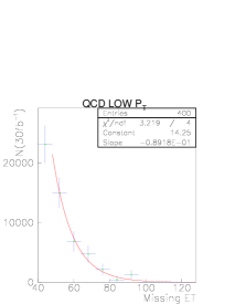
Figure 14: Exponential fit to the $E_{T}/\hskip 6.49994pt$ tail of the low $p_{T}$ QCD event sample.

Assuming uncorrelated gaussian errors on the fit and dividing the integral by the bin width gives an estimated $290\pm 450$ in the tail above 100​ GeV, meaning that less than $10^{3}$ events pass the cut at 95% confidence level, yielding a rejection factor for these events of at least 130 by the $E_{T}/\hskip 6.49994pt$ cut. Applying this rejection factor to the estimated $10^{6}$ events in the $p_{T}<100\mbox{\!\ GeV}$ QCD sample and adding up yields a maximum of $(1+7.5)\times 10^{3}<10^{4}$ QCD events with $p_{T}<150\mbox{\!\ GeV}$ remaining after the cut. Henceforth we refer to these $10^{4}$ events, combined, as the low-$p_{T}$ (QCD) sample.

5.3.2 Hard Leptons and Jets

As mentioned, a typical signature for SUSY is the large number of jets obtained. This, when combined with (possible) violation of Lepton Number, may well be accompanied by a large lepton multiplicity, and so it makes good sense to combine the analysis here. The lepton multiplicities (iso. muons + iso. electrons) in events with $E_{T}/\hskip 6.49994pt>100\mbox{\!\ GeV}$ are shown in figures 5.3.2a (SM) and 5.3.2b (mSUGRA $P_{9}$ MSSM, LLE, and LQD), and an overwiev of the distributions in the other scenarios investigated are shown in 5.3.2c. Jet multiplicities are shown in figure 5.3.2. One sees the larger relative lepton multiplicity in LLE scenarios and the larger relative jet multiplicity in LQD scenarios. Finally, the “box” plots in figure 5.3.2 show the correlations between the number of leptons and the number of jets with large boxes meaning that a large fraction of events have the corresponding combination of $N_{lep}$ and $N_{jets}$ and small boxes meaning that a small fraction of events have the corresponding combination.

Figure 15: a) and b): Lepton multiplicities in the SM and $P_{9}$ of events surviving the cut on $E_{T}/\hskip 6.49994pt$. The numbering of the bins is such that the events with 0 leptons are in the bin to the right of the number 0. c): Fractional distributions of events in all scenarios investigated.

Figure 16: a) and b): Jet multiplicities in the SM and $P_{9}$ of events surviving the cut on $E_{T}/\hskip 6.49994pt$. c): Fractional distributions of events in all scenarios investigated.

c)

a)	b)

c)

Figure 17: Lepton versus jet multiplicity (see text) in the SM and mSUGRA $P_{9}$ of events surviving the cut on $E_{T}/\hskip 6.49994pt$. The numbering of the bins is such that the events with 0 leptons are in the bin to the right of the number 0. The cuts investigated correspond to cutting out the lower left corner of each plot.

Based on these distributions, it seems reasonable to require at least $N_{J}$ jets, at least $(N_{J}-1)$ jets and at least 1 lepton, at least $(N_{J}-2)$ jets and at least 2 leptons, or at least 3 leptons. Values for $N_{J}=8-11$ have been investigated. Results are presented in table 5.3.2. For the $p_{T}<100\mbox{\!\ GeV}$ QCD sample, applying the rejection factor of 8.5 found for the high $p_{T}$ sample gives an estimated $900$ events at most remaining after the cut.

EVENTS PASSING CUTS ON N${}_{\mbox{\scriptsize jets}}$ AND N${}_{\mbox{\scriptsize leptons}}$.

Table 10: Events passing cuts on $N_{\mbox{\scriptsize jets}}$ and $N_{\mbox{\scriptsize leptons}}$ for several choices of jet cutoff, $N_{J}$ (see text). In addition, the requirement that each event pass the $E_{T}/\hskip 6.49994pt$ cut was imposed. The selected cut is marked in bold, and the ratio of events surviving after this cut to events surviving before this cut is shown for each model. A very good rejection factor for SM events is obtained. The reason for this is plain to see in figure 5.3.2. Cutting out the lower left corner in those plots takes away the majority of $Z/W$ events, and also a significant reduction in QCD and $t\bar{t}$ events is obtained. For the SM, the (gaussian) uncertainty due to the limited event sample is also shown.

As for the $E_{T}/\hskip 6.49994pt$ cuts, it is not at all surprising that the MSSM is here the model which does the worst. After all, the MSSM has a lot of $E_{T}/\hskip 6.49994pt$ exactly because the LSP escapes and does not give rise to extra jets and/or leptons. Note also that we have power to discriminate between MSSM, $R$/  with dominant LQD terms, or $R$/  with dominant LLE terms in these variables. This, however, is saved for the neural network analysis below.

Additional variables which are obvious as discriminators when studying the decays of heavy particles are (transverse) momenta of the hardest jets and leptons in the event. The transverse momenta of the four hardest jets and the two hardest leptons are therefore also used as inputs in the neural net analysis. For events with less than 4 jets and/or less than 2 leptons, the value 0 is assigned to the “missing” jet and lepton $p_{T}$’s. In the cut-based analysis, we simply use the $p_{T}$ of the hardest object in the event, $p_{T}^{hard}$. The SM and $P_{9}$ distributions for this variable are shown in figure 5.3.2. Cuts at $p_{T}^{hard}=100,150,200$, and $250$ were investigated with results as shown in table 11.

Figure 18: $p_{T}$ distribution for hardest object in SM and SUSY, normalized to 30​ fb^-1 of data taking. Events shown are the ones surviving previous cuts.

c)

EVENTS PASSING CUTS ON $p_{T}^{\mbox{\scriptsize hard}}$. SM $P_{9}$ MSSM $P_{9}$ LLE $P_{9}$ nLLE $P_{9}$ LQD $P_{9}$ nLQD $p_{T}^{hard}=100$ $(180\pm 10)$ k 220 k 410 k 380 k 270 k 290 k $p_{T}^{hard}=150$ $(140\pm 10)$ k 200 k 390 k 370 k 270 k 280 k $p_{T}^{hard}=200$ $(110\pm 5)$ k 180 k 360 k 330 k 250 k 260 k $p_{T}^{hard}=250$ $(85\pm 4)$ k 140 k 300 k 270 k 210 k 220 k $\frac{N_{\mbox{\tiny post}}}{N_{\mbox{\tiny pre}}}$ 0.57 0.80 0.86 0.85 0.90 0.90

Table 11: Events passing cuts on $p_{T}^{\mbox{\scriptsize hard}}$ for several choices of cut value. The selected cut is marked in bold, and the ratio of events surviving after this cut to events surviving before this cut is shown for each model.

Due to the higher resonance masses, the $P_{9}$ scenarios escape these cuts almost with impunity. The ratio of events surviving before and after the cut is even better for the rest of the mSUGRA points.

After the cut on hardest object, only 1 $Z/W$ event remained in the sample (out of $5\times 10^{7}$ generated). As is apparent from figure 5.3.2a, it would clearly be nonsense to fit the $P^{hard}_{T}$ distribution of $Z/W$ events to thereby obtain an estimate. Rather, we use the procedure recommended by [europhys] that a conservative upper bound on the number, $N$, passing the cut is given by the mean of that Poisson distribution which yields a 5% chance of giving only one event or less surviving the cut. This gives an estimate for $N<4.75$ at 95% confidence level, translating to $3400$ events after 30​ fb^-1 of data taking. With respect to the rejection factor expected for these events under subsequent cuts, we adopt a slightly pessimistic assumption, reducing the number of events by the same factor as the double gauge events ($ZZ/ZW/WW$). Before leaving the $Z/W$ events, we take one more look at figure 5.3.2a. It is here evident that there are 3 events just below the cut, and one might argue that our estimate of 3400 events is therefore likely to be too optimistic. This argument is incorrect since by using that knowledge we would invalidate the statistical approach just used. As long as the cut was not tuned to lie exactly above these events (and 200 was chosen only for its being a nice round number), the Poisson approach is statistically sound.

For the low-$p_{T}$ QCD events, the low rejection factor, 1.07, found for the high $p_{T}$ sample gives an estimated negligible reduction of event numbers by the $p_{T}^{hard}$ cut. One must recall, however, that the high $p_{T}$ QCD sample consists entirely of events where the hard scattering gave rise to $p_{T}>150\mbox{\!\ GeV}$ in the CM of the scattering. It is therefore quite natural that almost no reduction is accomplished for these events by demanding that the $p_{T}$ of the hardest object in the event be larger than 200​ GeV. For the low-$p_{T}$ QCD sample, we expect the reduction from this cut to be significantly greater, yet to be conservative, we use the same rejection as for the high $p_{T}$ sample, yielding maximally 420 events remaining.

5.3.3 LSP Decay Signature

The $R$/  scenarios give us one extra possible signature for SUSY events which is not present in the $R$-conserving cases, LSP decay. Out of necessity, we shall here focus on the case of a neutralino LSP. This means that we are looking for 3-body decays, a more difficult situation than for 2-body decays. It is, of course, impossible to say whether the lightest neutralino decays into $qq\nu$, $qq\ell$, or $\ell\ell\nu$ without making assumptions about the relative coupling strengths, something which is obviously not acceptable when one is interested in defining as general a search strategy as possible. Whatever coupling is dominant, there are maximally two neutrinos in an event with double neutralino decay (see section LABEL:sec:lspdecays). One would therefore expect to see at least 4 hard jets/leptons with energies not greatly differing from each other. We therefore introduce the following measure for this “4-object energy correlation”:

$$E_{4C}\equiv\frac{1}{3}(\frac{E_{4}}{E_{3}}+\frac{E_{3}}{E_{2}}+\frac{E_{2}}{E_{1}})$$ (35)

where $E_{1-4}$ are the energies of the 4 hardest objects (leptons or jets) in the event ordered in energy, the hardest being $E_{1}$. Events with $N_{lep}+N_{jet}<4$ are assigned the value zero. Following the above line of reasoning we would expect the SUSY events to have 4-object correlations close to 1. In contrast, there is no reason to expect this kind of correlation in e.g. $Z/W$ or QCD events. Also, a large number of double gauge events will have low or zero values since two gauge bosons decaying leptonically at most produce 4 hard objects in the detector. The $t\bar{t}$ events, however, are quite indistinguishable from many of the SUSY scenarios in this variable. Noting that the more massive a particle is, the larger the momentum kicks given to its decay products will be, one would expect that particles coming from the decays of objects heavier than the top would, on average, have larger $p_{T}$ than particles coming from top decays. We can use this to give the variable just defined some extra discriminating power against $t\bar{t}$ events. However, it comes at a cost. A look in table 4 reveals that $P_{9}$, for instance, has the LSP and several other SUSY particles lighter than the top. By giving the 4-object energy correlation some $p_{T}$ dependence, we will not only get rid of top events, we will also be throwing away signal events for SUSY scenarios with low-mass particles. This is not a serious drawback, since we can afford to loose a certain amount of signal in the low-mass scenarios due to the relatively high production cross sections. In return, we get a more pure signal for the heavier scenarios where we don’t have so many signal events and so require a better background rejection.

This is the basis for using the 4-object energy correlation multiplied by the average $p_{T}$ of the four hardest objects rather than the 4-object energy correlation alone, and so we introduce the $p_{T}$-weighted 4-object energy correlation:

$$P_{4C}\equiv\frac{1}{12}\left(\frac{E_{4}}{E_{3}}+\frac{E_{3}}{E_{2}}+\frac{E_{2}}{E_{1}}\right)(p_{T1}+p_{T2}+p_{T3}+p_{T4})$$ (36)

The suspicion that the low-mass scenarios will not do well in this variable is quickly verified by taking a look at figure 5.3.3c where peaks around 100​ GeV are seen for both $P_{9}$ and $F_{2}$ whereas the heavier scenarios show more flat distributions.

Figure 19: Distributions of $P_{4C}$ in the SM (a and b) and for mSUGRA $P_{9}$. All events used survive previous cuts.

c)

EVENTS PASSING CUTS ON P_4C. SM $P_{9}$ MSSM $P_{9}$ LLE $P_{9}$ nLLE $P_{9}$ LQD $P_{9}$ nLQD $P_{4C}>50$ $(108\pm 5)$ k 170 k 350 k 330 k 250 k 260 k $P_{4C}>75$ $(97\pm 5)$ k 160 k 330 k 310 k 240 k 250 k $P_{4C}>100$ $(79\pm 4)$ k 110 k 270 k 240 k 210 k 220 k $P_{4C}>125$ $(57\pm 4)$ k 72 k 190 k 170 k 160 k 160 k $\frac{N_{\mbox{\tiny post}}}{N_{\mbox{\tiny pre}}}$ 0.72 0.65 0.77 0.84 0.75 0.83

Table 12: Events passing cuts on $P_{4C}$ for SM and $P_{9}$ events surviving previous cuts, scaled to correspond to 30​ fb^-1 of data taking. The selected cut is marked in bold, and the ratio of events surviving after this cut to events surviving before this cut is shown for each model. One sees that the MSSM for does even worse than the SM for $P_{9}$, due to the absence of LSP decay. The rest of the mSUGRA points generally have acceptances close to 100% even for the MSSM. The only exception is $F_{2}$ which nonetheless lies above 80% in all cases.

For SUSY events where double LSP decay does not occur, note that there must be either one or more heavier particles decaying directly to SM particles or $R$-parity is conserved. In the first case, the $E_{i}/E_{j}$ will generally be lower, since jet/lepton energies are presumably not equal to so great an extent, but since heavier particles are decaying, the average $p_{T}$ will be larger, evening out the score. The $R$-conserving scenarios will look more like the SM in this variable, since no LSP decay occurs.

For the high-$p_{T}$ QCD and the double gauge events, rejection factors of 1.2 and 2.7, respectively, were found, yielding an estimated maximum of 350 low-$p_{T}$ QCD events and 1300 $Z/W$ remaining.

5.3.4 Thrust

One may intuitively understand that pair production involving less massive particles is liable to produce decay products which lie more “on a line” than processes involving more massive particles (where the decay products get larger momentum kicks). It is based on this that thrust is expected to be of use as a discriminating variable. Its value is defined as:

$$T=\mathrm{max}\left\{\frac{\sum_{i}|p_{i}\cdot\vec{n}|}{\sum_{i}|p_{i}|}\right\}$$ (37)

where $i$ runs over all particles in the event and $\vec{n}$ is a unit vector along an arbitrary axis. The axis which maximizes the expression is defined as the thrust axis. For a completely pencil-shaped event, the thrust value is 1, going down to 0.5 for an event where the momenta are evenly distributed throughout the detector. The thrust distributions for events satisfying the previous cuts are shown in figure 5.3.4.

Figure 20: Thrust distributions for SM processes and mSUGRA $P_{9}$. Observe that the QCD processes peak around 0.9 whereas $P_{9}$ peaks around 0.8. All events used survive previous cuts.

c) Cuts on $T<0.75$, $T<0.8$, $T<0.85$, and $T<0.90$ were investigated. Results are shown in table 13. The selected cut, $T<0.85$, is marked in bold.

EVENTS PASSING CUTS ON THRUST. SM $P_{9}$ MSSM $P_{9}$ LLE $P_{9}$ nLLE $P_{9}$ LQD $P_{9}$ nLQD $T<0.75$ $(10\pm 2)$ k 35 k 75 k 77 k 76 k 80 k $T<0.8$ $(24\pm 2)$ k 59 k 130 k 130 k 120 k 130 k $T<0.85$ $(40\pm 3)$ k 83 k 190 k 180 k 160 k 170 k $T<0.90$ $(62\pm 4)$ k 100 k 240 k 220 k 190 k 200 k $\frac{N_{\mbox{\tiny post}}}{N_{\mbox{\tiny pre}}}$ 0.51 0.73 0.69 0.74

Table 13: Events passing cuts on thrust for three values of thrust cutoff. The selected cut is marked in bold, and the ratio of events surviving after this cut to events surviving before this cut is shown for each model.

Rejection factors of 2.0 and 2.1 were obtained for the high $p_{T}$ QCD events and the double gauge sample, respectively, yielding 180 low-$p_{T}$ and 620 $Z/W$ events maximally remaining. Note that the $Z/W$ events would most likely have higher rejections under this cut than their double gauge counterparts, yet finding it difficult to quantify it, we do not include any additional suppression in the estimated number.

5.3.5 Oblateness and Circularity

Having defined the thrust axis for each event, one can take one step further and define Major and Minor axes in the plane perpendicular to the thrust axis in exactly the same way as thrust was defined:

$$\mbox{Major}=\mbox{max}\left\{\frac{\sum_{i}|p_{i}\cdot\vec{n}|}{\sum_{i}|p_{i}|}\right\}$$ (38)

where the maximum is now to be found perpendicular to the thrust axis. The Minor axis is then fixed as the axis perpendicular to both the thrust and Major axes, yet its value is computed exactly like thrust and Major values. These definitions of the Major and Minor axes, used at $e^{+}e^{-}$ colliders, get into trouble at a $pp$ machine like the LHC where variables sensitive to boosts along the $z$-axis are of very limited use. At $pp$ machines, one therefore defines the Major and Minor axes to lie orthogonal to the $z$-direction. This means that the Major axis will most often just be the projection of the thrust axis onto the $(x,y)$ plane. A measure for how “spread out” the event is in the $(x,y)$ plane is then given by subtracting the Minor from the Major, yielding the oblateness, $O$.

Essentially, the oblateness compares the fraction of $p_{T}$ in the direction where most $p_{T}$ is going and the fraction in the direction where least $p_{T}$ is going. An event with low oblateness is an event in which the $p_{T}$ is evenly distributed in the $(x,y)$ plane, and an event with high oblateness has its $p_{T}$ concentrated around the direction of the Major axis. Based on the same arguments that led us to introduce a $p_{T}$ dependence on the 4-object energy correlation, we expect SUSY events to have lower oblateness values than SM events, again with a tradeoff involved between signal loss at low SUSY masses and background rejection for higher SUSY masses. Distributions are shown in figure 5.3.5.

Figure 21: Oblateness distributions for SM processes and mSUGRA $P_{9}$. Observe that the QCD processes peak around 0.3 whereas $P_{9}$ peaks around 0.2. All events used survive previous cuts.

c) The effect of requiring the oblateness to be lower than 0.25, 0.3, 0.4, and 0.5 were investigated with results as given in table 14.

EVENTS PASSING CUTS ON OBLATENESS. SM $P_{9}$ MSSM $P_{9}$ LLE $P_{9}$ nLLE $P_{9}$ LQD $P_{9}$ nLQD $O<0.25$ $(17\pm 2)$ k 49 k 100 k 100 k 110 k 110 k $O<0.3$ $(24\pm 2)$ k 61 k 130 k 130 k 130 k 140 k $O<0.4$ $(34\pm 3)$ k 77 k 170 k 160 k 160 k 160 k $O<0.5$ $(40\pm 3)$ k 83 k 180 k 180 k 160 k 170 k $\frac{N_{\mbox{\tiny post}}}{N_{\mbox{\tiny pre}}}$ 0.84 0.92 0.88 0.95 0.91 0.95

Table 14: Events passing cuts on oblateness, normalized to 30​ fb^-1 of data taking. The selected cut is marked in bold, and the ratio of events surviving after this cut to events surviving before this cut is shown for each model.

A remarkable feature of the plots in figure 5.3.5c is that $P_{7}$, by far the heaviest mSUGRA point, has oblateness distributions which are broader than the lower-mass points. To understand the reason for this, a closer look was taken at the event histories for high-oblateness events in an nLLE $P_{7}$ scenario. A plausible explanation is that the extremely massive resonances in $P_{7}$ are produced more often than not with $p_{T}$ less than their masses. When we argued above that we would expect low oblateness for events containing more massive resonances, we implicitly assumed that the original direction of flight of the resonances would define the Major axis around which a non-zero Minor value would be generated by the decay of the resonances in proportion to their masses. But for resonances with masses as heavy as those found in $P_{7}$ (around 2​ TeV) this argument is turned upside down. At $P_{7}$, the (two-body) decays of the resonances produce momentum kicks of such large magnitudes that the original direction of flight can be completely erased, resulting in events looking roughly as depicted in figure 22 in the $(x,y)$ plane.

p7dec (160,60) arrow_len2.5mm 0.w,0.horigo 18.,0.xax 0.,18.yax 0.5w,0.5hc 0.1w,0.9hl1 0.3w,0.1hl3 0.9w,0.9hr1 0.7w,0.1hr3 plainorigo,xax plainorigo,yax fermionv1,l1 fermionv2,l3 fermionv1,r1 fermionv2,r3 fermionc,v1 fermionc,v2 label=$x$,label.dist=3,label.ang=-90,d.sh=tri,d.siz=5.,d.ang=-90xax label=$y$,label.dist=3,label.ang=180,d.sh=tri,d.siz=5.yax d.sh=hexagram,d.f=empty,d.siz=10.c d.sh=hexagram,d.f=empty,d.siz=6.v1 d.sh=hexagram,d.f=empty,d.siz=6.v2

Figure 22: Decay of a pair of extremely massive resonances, projected onto the $(x,y)$ momentum plane. Here, the decay products of the upper resonance have their momenta oriented predominantly along the $x$ axis, whereas the lower have larger fractions in the $z$ direction. In cases like this, the $x$ axis is close to being the Major with only little $p_{y}$ to generate a sizeable Minor.

The last event shape variable used in this work is the circularity, again a transverse version of a variable commonly used in $e^{+}e^{-}$ colliders, the sphericity [stirling96]. It is similar, but not identical, to 1 minus oblateness, in that events which have their $p_{T}$ evenly distributed in the transverse plane have high circularities and events with more uneven distributions low circularities. Having cut away the highest oblateness events, we try to catch a few more fish (background events) by cutting away the lowest circularity events as well. It is defined through the eigenvalues of the circularity matrix:

$$C=\frac{1}{\sum_{i}(p_{T}^{i})^{2}}\left[\begin{array}[]{cc}\displaystyle\sum_{i}(p_{x}^{i})^{2}&\displaystyle\sum_{i}p_{x}^{i}p_{y}^{i}\vspace*{2mm}\\ \displaystyle\sum_{i}p_{y}^{i}p_{x}^{i}&\displaystyle\sum_{i}(p_{y}^{i})^{2}\end{array}\right]$$ (39)

where $i$ runs over the reconstructed particles/jets in the event. The Circularity value is defined as twice the smallest eigenvalue of this matrix, making it a measure of the momentum fraction along the smaller of the principal axes. The distributions of events in the SM and SUSY surviving all previous cuts can be seen in figure 5.3.5. Taking a look at the very first few bins of the plots, one sees that circularity does indeed have some discriminating power beyond what was contained in the oblateness though it has not been possible to identify the cause. Cuts requiring a circularity greater than 0.05, 0.1, 0.15, and 0.20 were investigated with results shown in table 15.

Figure 23: Circularity distributions for SM and mSUGRA scenarios. Observe that the number of QCD events rises almost linearly with $C$ as one goes to smaller $C$ wheras the mSUGRA distributions peak around $0.1-0.2$. All events used survive previous cuts.

c)

EVENTS PASSING CUTS ON CIRCULARITY. SM $P_{9}$ MSSM $P_{9}$ LLE $P_{9}$ nLLE $P_{9}$ LQD $P_{9}$ nLQD $C>0.05$ $(29\pm 3)$ k 72 k 160 k 160 k 150 k 150 k $C>0.10$ $(24\pm 2)$ k 63 k 140 k 140 k 140 k 140 k $C>0.15$ $(20\pm 2)$ k 54 k 130 k 120 k 120 k 120 k $C>0.20$ $(16\pm 2)$ k 46 k 110 k 110 k 110 k 110 k $\frac{N_{\mbox{\tiny post}}}{N_{\mbox{\tiny pre}}}$ 0.68 0.81 0.86 0.84 0.87 0.86

Table 15: Events passing cuts on circularity, normalized to 30​ fb^-1 of data taking. The selected cut is marked in bold, and the ratio of events surviving after this cut to events surviving before the cut is shown for each model. Note that only 70 high-$p_{T}$ QCD events remain after the cut, and so the gaussian errors used here will be replaced by Poisson statistics in what follows.

A last thing worth noticing about the circularity is that whereas the thrust and the oblateness are linear in the momenta, circularity is quadratic. This means that two events which are identical in every respect except that one parton in the first event is replaced by two collinear partons with some sharing of the momentum in the other will not have the same circularities, since $(p_{a}+p_{b})^{2}\neq p_{a}^{2}+p_{b}^{2}$. This, in turn, means that the circularity is sensitive to uncertainties in the fragmentation model (where such splittings occur), in contrast to thrust and oblateness.

The combined rejection factors under the oblateness and circularity cuts were 1.7 and 1.6 for the high-$p_{T}$ QCD and double gauge events respectively. We thus estimate a maximum of 110 and 400 low-$p_{T}$ and single gauge events remaining, respectively. These numbers should be compared to 4000 $t\bar{t}$ and 20000 high-$p_{T}$ QCD events. Based on the 22 generated double gauge events remaining, an upper limit of 31.4 events can be set using the conservative Poisson estimate discussed in section 5.3.2, translating to a maximum of 20 events after $30\mbox{\!\ fb}^{-1}$ of data taking. One thus sees that the double gauge events are completely negligible as background, giving some justification of the earlier made statement that triple gauge events should also be negligible.

5.4 Pattern Recognition with Neural Networks

We now turn to the more specialized part of the analysis where we shall seek to extract signals for LLE, LQD, and MSSM SUSY scenarios separately using three neural networks trained to regocnize the specific event shapes associated with each scenario. The results of the analysis are presented in section 5.5. Here, we concentrate on the structure and function of neural networks and their application to the present problem, essentially one of pattern classification. Does this event “look” like a Standard Model event, or does it look like a SUSY event?

5.4.1 What Neural Networks Do

The first step in any analysis based on cuts is to find as optimal variables as possible to place cuts on, the second step to find the optimal placements of the cuts. What neural networks do is to learn which variables to use and where to place the cuts, based on a teaching sample of background and signal events. The simplest type of network consists of a single neuron which computes a linear combination of the input variables in the problem, in our case the discriminating variables just discussed. It then places a cut on this “activation level” and returns 1 if the activation was above the cut value and 0 otherwise. In our case, these two outputs would correspond to the event having been classified as either a signal or a background event. The learning algorithm then serves to adjust the coefficients in the linear combination and the placement of the cut according to the average error the network makes over the learning sample such that next time it goes over the sample it will classify more events correctly. The way this works is by a procedure called “gradient descent” where the network calculates the gradient of the error squared, or some other function that one wishes to minimize, with respect to each network parameter. It then adjusts each parameter, taking a small step in parameter space in the minimizing direction each time it has processed an event or, to decrease the effect of insignificant fluctuations, it sums up the required changes over a number of processed events before it applies them. This latter approach smoothes out the otherwise jittering movement of the network across parameter space, often allowing faster progress towards the minimum.

For gradient descent to work, note that the neuron cannot be allowed to compute a sharp cut on it its activation level, since the step function is discontinuous and hence not differentiable. Instead, one uses so-called sigmoidal functions which look like smoothed out versions of the step function. We consider these functions and the gradient descent algorithm in more detail below, yet let us first extend our network beyond just a single neuron.

In problems where the classification is not quite so easy that it can be performed using a cut on just one linear combination of the inputs, more neurons are needed, each one computing a sigmoidal function of its activation level, resulting in an output from each of these “cut neurons” between zero and one. These outputs then serve as inputs to the output neuron who sums them up in a new linear combination, the output neuron activation. In the present case, this activation is used directly as the network output, alternatively one may let the output neuron compute a function of its input. It remains that the computing power of the network lies in the cut neurons. A function may or may not be handy to apply to the output, but it will not increase the amount of information there is in the output value. It now also becomes apparent why the cut neurons are customarily referred to as hidden neurons. The world outside the network interacts with it by giving it input on the input neurons and by reading the output from the output neuron. The cut neurons communicate only with other neurons. Henceforth, we refer to these internal neurons as hidden neurons.

The function of a neural network is thus nothing but a number of smoothed cuts on the same number of linear combinations of the inputs, with the results of the cuts being used as variables in a last linear combination defining the output of the network – similar to what is being done in an ordinary cut-based analysis. The benefit is that neural networks automatically pick up correlations and anti-correlations between arbitrarily many of the input variables. A hypothetical example of high-dimensional correlations would be if we imagine that many signal events have high jet multiplicities when there is little $E_{T}/\hskip 6.49994pt$ in the event, but that they have very few jets when $E_{T}/\hskip 6.49994pt$ is high. Furthermore, let us suppose that, at high $E_{T}/\hskip 6.49994pt$  a certain fraction of signal events with few jets have high lepton multiplicities, but that at low $E_{T}/\hskip 6.49994pt$ high lepton multiplicities would be a characteristic of background events, unless there was also a high thrust in the event, or failing that at least a high oblateness. These correlations would of course follow from physical arguments related to the processes involved in shaping the hypothetical background and signal processes in this example, and linear combinations of the variables designed to make use of the correlations could be constructed and optimized manually, yet this would be an extremely time-consuming task considering the more than 50 different scenarios investigated in this work. Moreover, it is a task which neural networks are ideally suited for by construction.

5.4.2 Network Layout and Network Learning:

For each event to be processed, each of the discriminating variables defined above are presented as inputs to the network. Since the network is initizalized with random weights between 0 and 1, it is sensible to scale these inputs to typically lie in the range $[0,1]$ as well for faster learning. Otherwise, the input-to-hidden weights (the coefficients in the linear combination mentioned above) have to be corrected, possibly for a long time, until the right ball-park is found. The input normalizations used here are listed in table 16.

$i$	1	2	3	4	5	6	7
$\mathrm{In}_{i}$	$\displaystyle\frac{E_{T}/\hskip 6.49994pt}{200}$	$\displaystyle\frac{N_{\mathrm{jets}}}{15}$	$\displaystyle\frac{N_{\mu}^{\mathrm{iso}}}{5}$	$\displaystyle\frac{N_{e}^{\mathrm{iso}}}{5}$	$\displaystyle\frac{P_{4C}}{500}$	Thrust	Circularity
$i$	8	9	10	11	12	13	14
$\mathrm{In}_{i}$	Oblateness	$\displaystyle\frac{p_{T,\mathrm{jet}}^{1}}{100}$	$\displaystyle\frac{p_{,T\mathrm{jet}}^{2}}{100}$	$\displaystyle\frac{p_{T,\mathrm{jet}}^{3}}{100}$	$\displaystyle\frac{p_{T,\mathrm{jet}}^{4}}{100}$	$\displaystyle\frac{p_{T,\ell}^{1}}{100}$	$\displaystyle\frac{p_{T,\ell}^{2}}{100}$

Table 16: Inputs to the neural network and their normalizations. In the text, $i$ is used as an index denoting input neurons and $\mathrm{In}_{i}$ the value of the input variable as given in this table. Note that $\mathrm{In}_{i}$ is not necessarily identical to the output of the input neuron which we denote by $I_{i}$. $P_{4C}$ is defined in section 5.3.3, $p_{T\mathrm{jet}}^{1-4}$ are the transverse momenta of the four hardest jets, and $p_{T,\ell}^{1-2}$ of the two hardest leptons.

The hidden layer in most applied networks normally has fewer neurons than the input layer, representing that some generalization can already be made at this stage: it is not always necessary to form $N$ linear combinations of $N$ variables since some mutual interdependence can usually be eliminated. In the present analysis with 14 inputs, it is found that a network with 10 hidden neurons performs with negligible loss of discriminating power compared to networks with more hidden neurons. As described above, each hidden neuron computes a sigmoidal of its activation level, the name sigmoidal coming from the tilted $S$ shape of these functions. The particular sigmoidal used in this work is the logistic function (the most commonly used). This function assigns an output value for the $j$’th neuron in the hidden layer of:

$$\vspace*{2mm}H_{j}=\frac{1}{1+e^{-\sum_{i=1}^{N_{\mathrm{in}}}(I_{i}w_{ij})-\delta^{H}_{j}}}\vspace*{1mm}$$ (40)

where $I_{i}$ is the output of the $i$’th input neuron, $w_{ij}$ is the weight of the synapse connecting input $i$ to hidden neuron $j$, $\delta^{H}_{j}$ is a bias term for the hidden neuron, and $N_{\mathrm{in}}$ is the number of neurons in the input layer. Henceforth, we follow the convention that subscript $i$ refers to the input layer whereas subscript $j$ refers to the hidden layer. The slope of the sigmoid is sometimes also adjusted by introducing a “temperature”, $T$:

$$\vspace*{2mm}H_{j}=\frac{1}{1+e^{-\left(\sum_{i=1}^{N_{\mathrm{in}}}(I_{i}w_{ij})-\delta^{H}_{j}\right)/T_{j}}}\vspace*{1mm}$$ (41)

The effect of this modification is shown in figure 24.

Figure 24: The logistic (sigmoid) function for $T=2$ (dashed), $T=1$ (solid), and $T=0.5$ (dot-dashed).

However, since introducing a temperature different from unity simply corresponds to rescaling all the weights connecting to $H_{j}$ and the bias by a common factor $1/T_{j}$, there is nothing gained by introducing such a parameter. Moreover, the network becomes slower and there is the risk that it begins to oscillate between changing $T_{j}$ and rescaling the weights in the learning procedure, and so we stick with eq. (40). For the input neurons, only a bias is added to the value of the input variables:

$$I_{i}=\mathrm{In}_{i}-\delta^{I}_{i}$$ (42)

Taking one more look at figure 24 one also sees the reality of the earlier made comment that these functions look like smoothed out step functions and so can be regarded as smooth versions of cuts. The complete network layout looks as depicted in figure 25.

neural (320,150) arrow_len2mm i1,i2,i3,i4,i5,i6,i7 o 0.1w,0.43hv1 0.25w,0.43hv2 0.41w,0.43hv3 0.5w,0.43hv4 0.61w,0.43hv5 0.8w,0.43hv6 0.95w,0.7hwij 0.93w,0.43htm 0.95w,0.1hoj 0.93w,0htl 0.95w,1htr label=$I_{1}$,d.sh=circ,d.siz=0.08w,d.fill=empty,foreground=(0.7,,0,,0),label.dist=0i1 label=$I_{2}$,d.sh=circ,d.siz=0.08w,d.fill=empty,foreground=(0.8,,0.4,,0),label.dist=0i2 label=$...$i3 label=$I_{i}$,d.sh=circ,d.siz=0.08w,d.fill=empty,foreground=(0.7,,0.7,,0),label.dist=0i4 label=$...$i5 label=$I_{N_{\mathrm{in}}}$,d.sh=circ,d.siz=0.08w,d.fill=empty,foreground=(0.5,,0.7,,0),label.dist=0i6 label=$H_{1}$,d.sh=square,d.siz=0.075w,d.fill=empty,foreground=(0,,0.75,,0),label.dist=0v1 label=$H_{2}$,d.sh=square,d.siz=0.075w,d.fill=empty,foreground=(0,,0.7,,0.5),label.dist=0v2 label=$...$v3 label=$H_{j}$,d.sh=square,d.siz=0.075w,label.ang=-30,d.fill=empty,foreground=(0,,0.5,,0.8),label.dist=0v4 label=$...$v5 label=$H_{\!N_{\mathrm{hid}}}$,d.sh=square,d.siz=0.075w,d.fill=empty,foreground=(0,,0,,0.9),label.dist=0v6 label=$\mathcal{O}$,d.sh=circ,d.siz=0.08w,d.fill=empty,foreground=black,label.dist=0o fermion,right=0.3,foreground=(0.7,,0,,0)i1,v1 fermion,right=0.1,foreground=(0.7,,0,,0)i1,v2 fermion,foreground=(0.7,,0,,0)i1,v4 fermion,left=0.08,foreground=(0.7,,0,,0)i1,v6 fermion,right=0.3,foreground=(0.8,,0.4,,0)i2,v1 fermion,right=0.3,foreground=(0.8,,0.4,,0)i2,v2 fermion,left=0.05,foreground=(0.8,,0.4,,0)i2,v4 fermion,left=0.15,foreground=(0.8,,0.4,,0)i2,v6 fermion,right=0.3,foreground=(0.7,,0.7,,0)i4,v1 fermion,right=0.3,foreground=(0.7,,0.7,,0)i4,v2 fermion,foreground=(0.7,,0.7,,0)i4,v4 fermion,left=0.2,foreground=(0.7,,0.7,,0)i4,v6 fermion,right=0.2,foreground=(0.5,,0.7,,0)i6,v1 fermion,right=0.1,foreground=(0.5,,0.7,,0)i6,v2 fermion,left=0.05,foreground=(0.5,,0.7,,0)i6,v4 fermion,left=0.2,foreground=(0.5,,0.7,,0),label=$w_{ij}$,label.side=lefti6,v6 fermion,right=0.25,foreground=(0,,0.75,,0)v1,o fermion,right=0.1,foreground=(0,,0.7,,0.5)v2,o fermion,foreground=(0,,0.5,,0.8)v4,o fermion,left=0.15,foreground=(0,,0,,0.9),label=$o_{j}$,label.side=leftv6,o label=$I_{i}=\mathrm{In}_{i}-\delta^{I}_{i}$tr label=$H_{j}=\frac{1}{1+\exp(\sum_{i}I_{i}w_{ij}-\delta^{H}_{j})}$tm label=$\mathcal{O}=\frac{1}{N_{\mathrm{hid}}}\left(\sum_{j}H_{j}o_{j}-\delta^{O}\right)$tl

Figure 25: Layout of the neural networks used in the final part of the analysis (before brain-damage – see below).

5.4.3 Network Training

The neural networks used in this work all learn by adjusting their synaptic weights and biases in the direction which minimizes the error squared of the network, the error being defined on an event-by-event basis by:

$$e=t-\mathcal{O}$$ (43)

where $t$ is the target output (0 for background, 1 for signal), and $\mathcal{O}$ is the output that was actually obtained for the event.

As the name implies, the gradient descent learning algorithm [mcclelland89] consists of a learning rule defined by taking a step in weight space in the direction of the gradient of the (squared) error:

$$p\to p+\Delta p=p-\alpha\frac{\partial e^{2}}{\partial p}=p+2\alpha e\frac{\partial\mathcal{O}}{\partial p}$$ (44)

where $p$ represents any of the adjustable parameters in the network, $e$ is the error on the output, and $\alpha$ is a learning rate parameter specifying how large steps the network takes. This rule does not necessarily have to be applied immediately after each event in the learning sample has been processed. In order to wash out sharp, irregular changes called for from extreme events in the distributions, possibly pulling in opposite directions, we do better in accumulating the parameter changes over some processing period before invoking them. After the period, the accumulated change to each parameter is invoked, and the accumulated error is reset. In order to get as little statistical noise in the parameter changes as possible, the period was here set to be the number of events in the learning sample. Denoting event number by $n$, the learning rule above becomes:

$$p\to p+\Delta p=p+2\alpha\sum_{n}e(n)\frac{\partial\mathcal{O}(n)}{\partial p}$$ (45)

One further improvement can be made on the learning rule. Seeing as two successive changes to the parameters of the network often go in roughly the same direction in parameter space, we add a mixture of the last parameter change to the current change, something which often increases the learning speed of the network:

$$p\to p+\Delta p=p+2\alpha\sum_{n}e(n)\frac{\partial\mathcal{O}(n)}{\partial p}+\beta\Delta p^{\mathrm{last}}$$ (46)

where $\Delta p^{\mathrm{last}}$ is the change which was made after the previous period, and $\beta<1$ specifies the “inertia” of the system. We are now ready to specify the learning rules for each of the parameters of the network in fig. 25. These can be easily derived (using the chain rule).

$$\begin{array}[]{rclcrcl}\displaystyle\frac{\partial\mathcal{O}}{\partial\delta^{O}}&=&\displaystyle-1/N_{\mathrm{hid}}&&\displaystyle\frac{\partial\mathcal{O}}{\partial o_{j}}&=&\displaystyle\frac{H_{j}}{N_{\mathrm{hid}}}\vspace*{3mm}\\ \displaystyle\frac{\partial\mathcal{O}}{\partial\delta^{H}_{j}}&=&\displaystyle o_{j}H_{j}(H_{j}-1)&&\displaystyle\frac{\partial\mathcal{O}}{\partial w_{ij}}&=&\displaystyle\frac{o_{j}}{N_{\mathrm{hid}}}H_{j}(1-H_{j})I_{i}\vspace*{3mm}\\ \displaystyle\frac{\partial\mathcal{O}}{\partial\delta_{i}^{I}}&=&\displaystyle I_{i}(1-I_{i})\sum_{j}o_{j}H_{j}(H_{j}-1)w_{ij}&&\\ \end{array}$$ (47)

Replacing these quantities back into eq. (46) directly yields the required learning rules.

5.4.4 Optimal Brain Damage

As described above, the first derivates of the squared error with respect to the network parameters are used in training by gradient descent. It was shown by LeCun, Solla, and Denker [lecun90] that the second derivatives can be used to trim the network by getting rid of the most redundant parameters. This is desireable since redundant parameters are the ones that will eventually cause the network to overfit the sample space. This can have a severe effect on the generalizational ability of the network, i.e. its performance on data samples it has not been in contact with during the learning process. The idea of Optimal Brain Damage is to introduce a measure for how much the squared error will change as a result of deleting each network parameter. The parameters whose deletion will have the least effect can then be discarded if over-fitting is a problem. The measure proposed in [lecun90] is the saliency, defined for the network parameter $p$ as:

$$s_{p}=\frac{p^{2}}{2}\frac{\partial^{2}e^{2}}{\partial p^{2}}$$ (48)

This definition is appropriate when the learning process is near its end and the network is almost in the minimum (otherwise a more general formula would apply. See [lecun90]). The procedure is quite simple. One begins with a network that contains many parameters. One then trains it and deletes the parameters with lowest saliency. The resulting, “brain-damaged”, network is then retrained until it converges. This procedure is repeated until a satisfactory compromise between the mean squared error and the generalizational ability of the network is found. As a side benefit, the finished network contains fewer parameters and is therefore faster to run. What happens is typically that the smallest coefficients in the linear combinations forming the hidden neuron activations get thrown away while the larger coefficients are kept. The diagonal second derivates of the parameters for the present network are:

$$\frac{\partial^{2}e^{2}}{\partial(\delta^{I}_{i})^{2}} = \frac{2}{N_{\mathrm{hid}}}\left[\left(\sum_{j=1}^{N_{\mathrm{hid}}}\!w_{ij}H_{j}o_{j}(1\!-\!H_{j})\right)^{2}\!\!-e\left(\sum_{j=1}^{N_{\mathrm{hid}}}\!w_{ij}^{2}o_{j}H_{j}(1\!-\!H_{j}(3\!-\!2H_{j}))\right)\right]$$ (49)

$$\frac{\partial^{2}e^{2}}{\partial w_{ij}^{2}} = \frac{2}{N_{\mathrm{hid}}}I_{i}^{2}H_{j}o_{j}\left(o_{j}H_{j}(1-H_{j})^{2}+e(1-H_{j}(3-2H_{j}))\right)$$ (50)

$$\frac{\partial^{2}e^{2}}{\partial(\delta^{H}_{j})^{2}} = \frac{2}{N_{\mathrm{hid}}}H_{j}o_{j}\left(o_{j}H_{j}(1-H_{j})^{2}+e(1-H_{j}(3-2H_{j})))\right)$$ (51)

$$\frac{\partial^{2}e^{2}}{\partial o_{j}^{2}} = \frac{2H_{j}^{2}}{N_{\mathrm{hid}}}$$ (52)

$$\frac{\partial^{2}e^{2}}{\partial(\delta^{O})^{2}} = \frac{2}{N_{\mathrm{hid}}}$$ (53)

Each of the networks used thus started out with 14 inputs (= 14 biases), 10 hidden units (= 10 biases), 140 input-to-hidden synapses, 10 hidden-to-output synapses, and a bias on the output for a total of 175 parameters. Approximately a quarter of the parameters can be deleted with very little effect on the mean squared error of the networks over the learning samples, but with an increase in convergence rate and processing speed. An example of a finished, brain-damaged network, the one used for MSSM recognition, is illustrated in figure 26.

brain (400,100) thin in1,in2,in3,in4,in5,in6,in7,in8,in9,in10,in11,in12,in13,in14 arrow_len2.5mm 0.05w,0.3hh1 0.15w,0.3hh2 0.25w,0.3hh3 0.35w,0.3hh4 0.45w,0.3hh5 0.55w,0.3hh6 0.65w,0.3hh7 0.75w,0.3hh8 0.85w,0.3hh9 0.95w,0.3hh10 out label=$\delta$,label.dist=2in1 label=$\delta$,label.dist=2in2 label=$\delta$,label.dist=2in6 label=$\delta$,label.dist=2in8 label=$\delta$,label.dist=2in9 label=$\delta$,label.dist=2in10 label=$\delta$,label.dist=2in12 label=$\delta$,label.dist=2in14 label=$\delta$,label.dist=3h1 label=$\delta$,label.dist=3h2 label=$\delta$,label.dist=3h3 label=$\delta$,label.dist=5h4 label=$\delta$,label.dist=3h8 label=$\delta$,label.dist=2out plainin1,h1 plainin1,h2 plainin1,h3 plainin1,h4 plainin1,h6 plainin1,h8 plainin1,h9 plainin2,h2 plainin2,h3 plainin2,h4 plainin2,h6 plainin2,h9 plainin3,h1 plainin3,h2 plainin3,h4 plainin4,h1 plainin4,h3 plainin4,h6 plainin4,h8 plainin5,h1 plainin5,h3 plainin5,h4 plainin5,h8 plainin6,h1 plainin6,h2 plainin6,h3 plainin6,h4 plainin6,h5 plainin6,h6 plainin6,h7 plainin6,h8 plainin6,h9 plainin6,h10 plainin7,h2 plainin7,h4 plainin7,h6 plainin7,h7 plainin7,h8 plainin7,h9 plainin8,h1 plainin8,h2 plainin8,h3 plainin8,h4 plainin8,h6 plainin8,h7 plainin8,h8 plainin9,h3 plainin9,h4 plainin9,h5 plainin9,h6 plainin9,h7 plainin9,h8 plainin9,h9 plainin9,h10 plainin10,h2 plainin10,h3 plainin10,h4 plainin10,h5 plainin10,h6 plainin10,h7 plainin10,h8 plainin10,h9 plainin10,h10 plainin11,h1 plainin11,h2 plainin11,h3 plainin11,h4 plainin11,h5 plainin11,h6 plainin11,h7 plainin11,h8 plainin11,h10 plainin12,h1 plainin12,h2 plainin12,h3 plainin12,h4 plainin12,h6 plainin12,h7 plainin12,h8 plainin12,h9 plainin13,h1 plainin13,h2 plainin13,h3 plainin13,h5 plainin13,h6 plainin13,h7 plainin13,h8 plainin13,h9 plainin13,h10 plainin14,h1 plainin14,h2 plainin14,h3 plainin14,h4 plainin14,h6 plainin14,h8 plainin14,h9 plainin14,h10 plainh1,out plainh2,out plainh3,out plainh4,out plainh5,out plainh6,out plainh7,out plainh8,out plainh9,out plainh10,out

Figure 26: Sketch of the MSSM network after brain damage. Neurons with biases still on are shown with the symbol $\delta$. The numbering of the inputs goes from left to right.

To improve the convergence rate, two further improvements were made in the design. Firstly, a fixed learning rate is not optimal since there may be regions in “error space” which look like endless plateaus to one whose legs are not long enough. The network was therefore equipped with the ability to increase its learning rate if the relative change in the squared error (averaged over the learning sample) after a learning cycle is small. A little experimenting showed an error change of less than 5% from cycle to cycle to be a good indicator of when a larger learning rate was needed. Secondly, unlimited growth is not desireable. At the other side of a plateau, a mountaneous region may yet exist, and so a mechanism to decrease the rate is also included. If the error change is greater than zero, meaning that the error increases, the network “concludes” that it has taken too big a step, unlearns the direct effects of the last learning step (“direct” here meaning that the effects of the momentum term are not unlearned) and goes forward again with a smaller learning rate. After some more experimenting to reach a good balance between increase and decrease, this technique proved highly efficient, typically improving the convergence rate by factors of ten.

5.5 Results

As the last item on the agenda, results for signal extraction in all $L$/ -SUSY scenarios studied are now presented. For this purpose, three networks were constructed and trained to recognize MSSM, LLE, and LQD signals respectively. Approximately 8000 background events, scaled to represent approximately $10^{7}$ events in the learning algorithm, and 6000 signal events were used in each training process, all events required only to have passed the triggers. The relative numbers of signal and background events, as seen by the learning algorithm, are thus fairly similar to the post-trigger event numbers expected for SUSY cross sections around $10^{-10}$​ mb. For the LQD network, the background numbers were scaled by twice as much to obtain a better rejection factor in view of the less clean signatures of the LQD couplings. For each sample, half of the events were set aside as an independent sample on which the performance of the network was tested for over-fitting cycle by cycle. A typical learning curve is shown in figure 27, together with the gradually improving separation of the two distributions early on in the learning process (only discernible in colour).

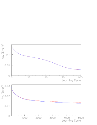
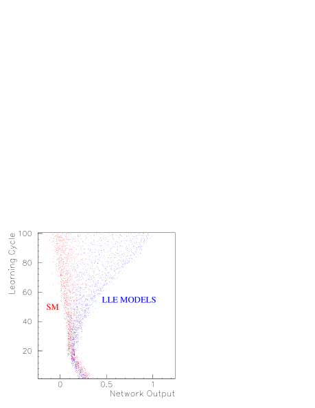
a)	b)

Figure 27: a) Learning Curves for the LLE network, average squared error versus learning cycle. The blue curve represents the average squared error on the learning sample and the red (dashed) the performance on the independent sample. b) learning cycle versus network output. Each red point represents an SM event and each blue point a SUSY event. In the beginning, the network is not capable of distinguishing between them, yet it quickly learns to separate the two distributions.

Selecting for each network events with network outputs above 0.9, we obtain a number of signal and background events for which we define the statistical significance of the signal (which we shall call the discovery potential) by:

$$P=\frac{S}{\sqrt{S+B}}$$ (54)

where $B$ should be understood as the number of background events, $N$, coming out of the analysis plus 1.64 standard deviations to account for the statistical uncertainty related to the limited number of generated events, 1.64 being chosen since 95% of a gaussian distributed event sample will lie below the mean plus 1.64$\sigma$. For low numbers of generated events, we use the conservative Poisson estimate discussed in section 5.3.2 to reach the same 95% confidence on $B$. If $P$ is above 5 for any of the networks, we draw the preliminary conclusion that a 5$\sigma$ discovery is possible.

In reality, $P$ should be corrected for QCD uncertainties and the effects of pile-up, and so we can only be confident that a $5\sigma$ discovery is possible if $P$ is somewhat larger than 5. Therefore, aside from working with the definition, eq. (54), we attempt to obtain a more believable estimate by including the effects of pile-up and QCD uncertainties in a very crude, ad hoc manner. To accomplish this, we now take a look at why eq. (54) is a reasonable quantity to use for the statistical significance. When we ask for a 5$\sigma$ discovery, we are really asking that the background hypothesis be more than 5 standard deviations away from the number of observed events. Assuming the event numbers to be gaussian distributed, we arrive at the requirement:

$$\begin{array}[]{lrcl}&N_{obs}-5\sigma_{N_{obs}}&>&B\\ \implies&S+B-5\sqrt{S+B}&>&B\\ \implies&P=\displaystyle\frac{S}{\sqrt{S+B}}&>&5\end{array}$$ (55)

Note that other definitions are also possible. One could equally well ask that the background plus 5$\sqrt{B}$ should be less than the observed number, resulting in more optimistic $P$ values for larger numbers of signal events.

The problem with pile-up lies in that the ratio of signal to background events passing the analysis is too optimistic. To include an estimate of the reduction of this ratio, we rewrite eq. (55) to:

$$P=\frac{\sqrt{S}}{\sqrt{1+B/S}}>5$$ (56)

where we include the effects of pile-up by multiplying $B/S$ by some factor. That twice as many background events per signal event could be passing the analysis if pile-up was included seems a reasonably pessimistic guess. Furthermore, assuming that the intrinsic uncertainty on both $S$ and $B$ coming from uncertainties on QCD parameters will, to a first approximation, work in the same direction and with a comparable magnitude for both $B$ and $S$, we expect that the denominator in the above formula is not affected by this uncertainty, and so we include the QCD-related uncertainties by reducing the number of signal events in the numerator by a factor of 1.5. This yields the following form for the “corrected discovery potential”:

$$P_{corr}=\frac{S}{\sqrt{1.5S+3B}}$$ (57)

Both $P$ and $P_{corr}$ will be listed in the results below.

As was indeed the purpose, the network classifications gave very few background events with outputs above 0.9. The response to background events surviving the cut-based analysis over the entire output range is shown in figure 28.

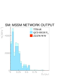
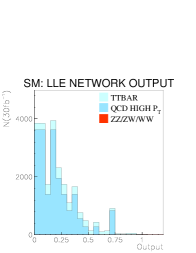
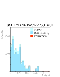
Figure 28: Network outputs for background events. As for the previous plots, the numbers of double gauge events are too small to be visible. We include them in the legend merely to signify that they have been taken into account.

For all three networks, no QCD events survived the cut at 0.9. Knowing that the network is a highly non-trivial function, especially near 0 and 1, we do not attempt to fit the distribution. Rather, we note that zero events has less than 5% probability of coming from a distribution with mean larger than 2.99. Adopting and scaling this estimate yields the numbers given in table 17.

Process	$B_{MSSM-net}$	$B_{LLE-net}$	$B_{LQD-net}$
Low-$p_{T}$ QCD	5	5	5
High-$p_{T}$ QCD	840	840	840
Z/W	150	150	150
$t\bar{t}$	210	140	100
ZZ/ZW/WW	5	5	5
Total SM	1210	1140	1100

Table 17: Estimated maximal event numbers remaining after network cuts. Maximal here means that the Poisson estimate discussed in section 5.3.2 has been used to estimate $B$ as the mean of the distribution that would result in 5% probability of getting the number of generated events or less which remained in the event samples actually used. Since any distribution with a higher mean would have less than 5% probability of resulting in the generated numbers, this is equivalent to saying that we have 95% confidence in the numbers here being maximal.

The same kind of Poisson estimate was used for the double gauge events, mainly to estimate the rejection factor which should be applied to the remaining single gauge events. Also for the $t\bar{t}$ event sample, the Poisson estimate was used where the number of generated events remaining was less than 100, else the gaussian 95% confidence estimate, $B<N+1.64\sqrt{N}$.

The total number of background events passing each network, as listed in table 17, can now be used as upper limits on the quantity $B$ entering eqs. (54) and (57) by which we have defined the discovery potential and the corrected discovery potential, respectively. Typically, around $500-1000$ signal events remain after cuts for $P_{2}$, $P_{12}$, and $F_{2}$. More remain for $P_{9}$ because of the larger cross section, but not nearly as large a fraction as for the other scenarios. $P_{7}$, of course, was impossible from the start, with only 114 events expected after $30\mbox{\!\ fb}^{-1}$, yet one should keep in mind that large values of the $R$/  couplings can lead to a significant increase in the production cross section for the heavy-mass points, $P_{7}$ and $F_{2}$, due to single sparticle production not included in the present analysis. For a hadron machine like the LHC, this effect will be largest in the LQD scenarios since single squark production will then be possible.

The discovery potentials, corrected and uncrrected, for all scenarios are given in table LABEL:tab:discoverypotential. The labelling of the models in the table should be self-explanatory to a large extent. The subscripts $a$, $b$, and $n$ refer to the column labels in table 5 where the $L$/  scenarios were defined, so that $a$ and $b$ are the constant coupling scenarios, and $n$ is the scenario with natural (hierarchical) couplings. This distinction, of course, does not exist for the MSSM where no lepton number violating couplings exist. The individual numbers in the table are not extremely interesting, except for the quite significant fact that, except for $P_{7}$, they are all above 5 for at least one of the network types. It is also of some interest to note that signals can be extracted reliably for the mixed (LLE+LQD) scenarios which neither entered in the cut optimization nor in the network training. Our estimate of the LHC discovery potential in the case of Lepton Number Violating SuperGravity scenarios is thus that a $5\sigma$ discovery is possible for cross sections down to at least $10^{-10}\!\ \mathrm{mb}$ with 95% certainty when the effects of pile-up and uncertainties on QCD parameters are neglected. Depending on whether our reduced estimate of the discovery potential does a reasonable job, these uncertainties should not be able to affect this general conclusion, yet one sees that there could be cause for concern for models with non-zero LQD couplings in SUSY scenarios of the $F_{2}$ type. As mentioned above, however, one would expect single sparticle production to be enhancing the cross section for this model for large values of the $\lambda^{\prime}$ couplings whereas low values would mean longer LSP lifetimes and hence either secondary vertices or an MSSM-like signature if the LSP escapes detection altogether. In the first case, we would have an extra discriminating variable, and in the second we note that even in the present analysis (in which the cuts were not optimized with the MSSM in mind) we have a reduced discovery potential of up to $6.5\sigma$ for the $F_{2}$ MSSM model.

NETWORK SUSY MSSM LLE LQD Point $P/P_{corr}$ $P/P_{corr}$ $P/P_{corr}$ $P_{2a}^{\mbox{\tiny LLE }}$ $24.3/16.2$ $25.5/17.1$ $25.4/17.1$ $P_{2b}^{\mbox{\tiny LLE }}$ $24.5/16.3$ $25.8/17.3$ $25.7/17.3$ $P_{2n}^{\mbox{\tiny LLE }}$ $23.2/15.4$ $24.7/16.5$ $24.3/16.3$ $P_{7a}^{\mbox{\tiny LLE }}$ $0.7\color[rgb]{0,0,0}/\color[rgb]{1,0,0}0.4$ $0.7\color[rgb]{0,0,0}/\color[rgb]{1,0,0}0.4$ $0.8\color[rgb]{0,0,0}/\color[rgb]{1,0,0}0.5$ $P_{7b}^{\mbox{\tiny LLE }}$ $0.8\color[rgb]{0,0,0}/\color[rgb]{1,0,0}0.4$ $0.8\color[rgb]{0,0,0}/\color[rgb]{1,0,0}0.4$ $0.8\color[rgb]{0,0,0}/\color[rgb]{1,0,0}0.5$ $P_{7n}^{\mbox{\tiny LLE }}$ $0.7\color[rgb]{0,0,0}/\color[rgb]{1,0,0}0.4$ $0.7\color[rgb]{0,0,0}/\color[rgb]{1,0,0}0.4$ $0.8\color[rgb]{0,0,0}/\color[rgb]{1,0,0}0.5$ $P_{9a}^{\mbox{\tiny LLE }}$ $191/153$ $315/256$ $218/176$ $P_{9b}^{\mbox{\tiny LLE }}$ $190/153$ $316/256$ $218/176$ $P_{9n}^{\mbox{\tiny LLE }}$ $166/133$ $257/208$ $169/135$ $P_{12a}^{\mbox{\tiny LLE }}$ $23.4/15.5$ $25.6/17.2$ $25.5/17.2$ $P_{12b}^{\mbox{\tiny LLE }}$ $23.4/15.5$ $25.5/17.2$ $25.5/17.2$ $P_{12n}^{\mbox{\tiny LLE }}$ $21.8/14.4$ $24.2/16.2$ $24.3/16.3$ $F_{2a}^{\mbox{\tiny LLE }}$ $11.3/7.0$ $14.0/8.8$ $13.3/8.4$ $F_{2b}^{\mbox{\tiny LLE }}$ $11.2/6.9$ $13.7/8.7$ $13.1/8.2$ $F_{2n}^{\mbox{\tiny LLE }}$ $9.9/6.1$ $12.4/7.8$ $12.3/7.7$
$P_{2a}^{\mbox{\tiny LQD }}$	$20.9/13.7$	$24.3/16.2$	$24.8/16.6$
$P_{2b}^{\mbox{\tiny LQD }}$	$21.4/14.1$	$24.7/16.5$	$25.3/17.0$
$P_{2n}^{\mbox{\tiny LQD }}$	$21.5/14.1$	$23.3/15.5$	$24.2/16.2$
$P_{7a}^{\mbox{\tiny LQD }}$	$1.0\color[rgb]{0,0,0}/\color[rgb]{1,0,0}0.6$	$1.0\color[rgb]{0,0,0}/\color[rgb]{1,0,0}0.6$	$1.1\color[rgb]{0,0,0}/\color[rgb]{1,0,0}0.6$
$P_{7b}^{\mbox{\tiny LQD }}$	$1.0\color[rgb]{0,0,0}/\color[rgb]{1,0,0}0.6$	$1.0\color[rgb]{0,0,0}/\color[rgb]{1,0,0}0.6$	$1.1\color[rgb]{0,0,0}/\color[rgb]{1,0,0}0.7$
$P_{7n}^{\mbox{\tiny LQD }}$	$1.0\color[rgb]{0,0,0}/\color[rgb]{1,0,0}0.6$	$1.0\color[rgb]{0,0,0}/\color[rgb]{1,0,0}0.6$	$1.1\color[rgb]{0,0,0}/\color[rgb]{1,0,0}0.6$
$P_{9a}^{\mbox{\tiny LQD }}$	$116/91.6$	$153/122$	$125/99.0$
$P_{9b}^{\mbox{\tiny LQD }}$	$113/88.7$	$151/121$	$123/97.6$
$P_{9n}^{\mbox{\tiny LQD }}$	$113/88.5$	$131/104$	$110/86.6$
$P_{12a}^{\mbox{\tiny LQD }}$	$15.7/10.0$	$19.2/12.5$	$20.9/13.7$
$P_{12b}^{\mbox{\tiny LQD }}$	$15.8/10.1$	$19.4/12.6$	$21.1/13.9$
$P_{12n}^{\mbox{\tiny LQD }}$	$16.6/10.6$	$18.6/12.1$	$20.9/13.8$
$F_{2a}^{\mbox{\tiny LQD }}$	$7.0/\color[rgb]{1,0,0}4.2$	$9.5/\color[rgb]{0.6,0.05,0.05}5.9$	$10.5/6.5$
$F_{2b}^{\mbox{\tiny LQD }}$	$7.0/\color[rgb]{1,0,0}4.2$	$9.4/\color[rgb]{0.6,0.05,0.05}5.8$	$10.5/6.5$
$F_{2n}^{\mbox{\tiny LQD }}$	$6.9/\color[rgb]{1,0,0}4.2$	$8.8/\color[rgb]{0.6,0.05,0.05}5.4$	$10.3/6.4$

& NETWORK SUSY MSSM LLE LQD Point $P/P_{corr}$ $P/P_{corr}$ $P/P_{corr}$ $P_{2}^{\mbox{\tiny MSSM }}$ $10.4/6.4$ $10.2/6.3$ $10.2/6.3$ $P_{7}^{\mbox{\tiny MSSM }}$ $0.2\color[rgb]{0,0,0}/\color[rgb]{1,0,0}0.1$ $0.2\color[rgb]{0,0,0}/\color[rgb]{1,0,0}0.1$ $0.2\color[rgb]{0,0,0}/\color[rgb]{1,0,0}0.1$ $P_{9}^{\mbox{\tiny MSSM }}$ $136/108$ $121/95.9$ $93.5/72.8$ $P_{12}^{\mbox{\tiny MSSM }}$ $16.1/10.3$ $15.5/9.9$ $16.1/10.3$ $F_{2}^{\mbox{\tiny MSSM }}$ $9.4/\color[rgb]{0.6,0.05,0.05}5.8$ $9.7/\color[rgb]{0.6,0.05,0.05}6.0$ $10.5/6.5$