Chapter 1 The Standard Model in 2001

Jonathan L. Rosner
Enrico Fermi Institute and Department of Physics

University of Chicago

5640 South Ellis Avenue, Chicago IL 60637, USA

1 Introduction

The “Standard Model” of elementary particle physics encompasses the progress that has been made in the past half-century in understanding the weak, electromagnetic, and strong interactions. The name was apparently bestowed by my Ph. D. thesis advisor, Sam B. Treiman, whose dedication to particle physics kindled the light for so many of his students during those times of experimental and theoretical discoveries. These lectures are dedicated to his memory.

As graduate students at Princeton in the 1960s, my colleagues and I had no idea of the tremendous strides that would be made in bringing quantum field theory to bear upon such a wide variety of phenomena. At the time, its only domain of useful application seemed to be in the quantum electrodynamics (QED) of photons, electrons, and muons.

Our arsenal of techniques for understanding the strong interactions included analyticity, unitarity, and crossing symmetry (principles still of great use), and the emerging SU(3) and SU(6) symmetries. The quark model (Gell-Mann 1964, Zweig 1964) was just beginning to emerge, and its successes at times seemed mysterious. The ensuing decade gave us a theory of the strong interactions, quantum chromodynamics (QCD), based on the exchange of self-interacting vector quanta. QCD has permitted quantitative calculations of a wide range of hitherto intractable properties of the hadrons (Lev Okun’s name for the strongly interacting particles), and has been validated by the discovery of its force-carrier, the gluon.

In the 1960s the weak interactions were represented by a phenomenological (and unrenormalizable) four-fermion theory which was of no use for higher-order calculations. Attempts to describe weak interactions in terms of heavy boson exchange eventually bore fruit when they were unified with electromagnetism and a suitable mechanism for generation of heavy boson mass was found. This electroweak theory has been spectacularly successful, leading to the prediction and observation of the $W$ and $Z$ bosons and to precision tests which have confirmed the applicability of the theory to higher-order calculations.

In this introductory section we shall assemble the ingredients of the standard model — the quarks and leptons and their interactions. We shall discuss both the theory of the strong interactions, quantum chromodynamics (QCD), and the unified theory of weak and electromagnetic interactions based on the gauge group SU(2) $\otimes$ U(1). Since QCD is an unbroken gauge theory, we shall discuss it first, in the general context of gauge theories in Section 2. We then discuss the theory of charge-changing weak interactions (Section 3) and its unification with electromagnetism (Section 4). The unsolved part of the puzzle, the Higgs boson, is treated in Section 5, while Section 6 concludes.

These lectures are based in part on courses that I have taught at the University of Minnesota and the University of Chicago, as well as at summer schools (e.g., Rosner 1988, 1997). They owe a significant debt to the fine book by Quigg (1983).

1.1 Quarks and leptons

The fundamental building blocks of strongly interacting particles, the quarks, and the fundamental fermions lacking strong interactions, the leptons, are summarized in Table 1. Masses are as quoted by the Particle Data Group (2000). These are illustrated, along with their interactions, in Figure 1. The relative strengths of the charge-current weak transitions between the quarks are summarized in Table 2.

Figure 1: Patterns of charge-changing weak transitions among quarks and leptons. The strongest inter-quark transitions correspond to the solid lines, with dashed, dot-dashed, and dotted lines corresponding to successively weaker transitions.

Table 1: The known quarks and leptons. Masses in GeV except where indicated otherwise. Here and elsewhere we take $c=1$.

Quarks				Leptons
Charge $2/3$		Charge $-1/3$		Charge $-1$		Charge 0
	Mass		Mass		Mass		Mass
$u$	0.001–0.005	$d$	0.003–0.009	$e$	0.000511	$\nu_{e}$	$<3$ eV
$c$	1.15–1.35	$s$	0.075–0.175	$\mu$	0.106	$\nu_{\mu}$	$<190$ keV
$t$	$174.3\pm 5.1$	$b$	4.0–4.4	$\tau$	1.777	$\nu_{\tau}$	$<18.2$ MeV

Table 2: Relative strengths of charge-changing weak transitions.

Relative	Transition	Source of information
amplitude		(example)
$\sim$ 1	$u\leftrightarrow d$	Nuclear $\beta$-decay
$\sim$ 1	$c\leftrightarrow s$	Charmed particle decays
$\sim 0.22$	$u\leftrightarrow s$	Strange particle decays
$\sim 0.22$	$c\leftrightarrow d$	Neutrino prod. of charm
$\sim 0.04$	$c\leftrightarrow b$	$b$ decays
$\sim 0.003$–0.004	$u\leftrightarrow b$	Charmless $b$ decays
$\sim$ 1	$t\leftrightarrow b$	Dominance of $t\to Wb$
$\sim 0.04$	$t\leftrightarrow s$	Only indirect evidence
$\sim 0.01$	$t\leftrightarrow d$	Only indirect evidence

The quark masses quoted in Table 1 are those which emerge when quarks are probed at distances short compared with 1 fm, the characteristic size of strongly interacting particles and the scale at which QCD becomes too strong to utilize perturbation theory. When regarded as constituents of strongly interacting particles, however, the $u$ and $d$ quarks act as quasi-particles with masses of about 0.3 GeV. The corresponding “constituent-quark” masses of $s$, $c$, and $b$ are about 0.5, 1.5, and 4.9 GeV, respectively.

1.2 Color and quantum chromodynamics

The quarks are distinguished from the leptons by possessing a three-fold charge known as “color” which enables them to interact strongly with one another. (A gauged color symmetry was first proposed by Nambu 1966.) We shall also speak of quark and lepton “flavor” when distinguishing the particles in Table 1 from one another. The experimental evidence for color comes from several quarters.

1. Quark statistics. One of the lowest-lying hadrons is a particle known as the $\Delta^{++}$, an excited state of the nucleon first produced in $\pi^{+}p$ collisions in the mid-1950s at the University of Chicago cyclotron. It can be represented in the quark model as $uuu$, so it is totally symmetric in flavor. It has spin $J=3/2$, which is a totally symmetric combination of the three quark spins (each taken to be 1/2). Moreover, as a ground state, it is expected to contain no relative orbital angular momenta among the quarks.

This leads to a paradox if there are no additional degrees of freedom. A state composed of fermions should be totally antisymmetric under the interchange of any two fermions, but what we have described so far is totally symmetric under flavor, spin, and space interchanges, hence totally symmetric under their product. Color introduces an additional degree of freedom under which the interchange of two quarks can produce a minus sign, through the representation $\Delta^{++}\sim\epsilon_{abc}u^{a}u^{b}u^{c}$. The totally antisymmetric product of three color triplets is a color singlet.

2. Electron-positron annihilation to hadrons. The charges of all quarks which can be produced in pairs below a given center-of-mass energy is measured by the ratio

$$R\equiv\frac{\sigma(e^{+}e^{-}\to{\rm hadrons})}{\sigma(e^{+}e^{-}\to\mu^{+}\mu^{-})}=\sum_{i}Q_{i}^{2}~{}~{}~{}.$$ (1)

For energies at which only $u\bar{u}$, $d\bar{d}$, and $s\bar{s}$ can be produced, i.e., below the charmed-pair threshold of about 3.7 GeV, one expects

$$R=N_{c}\left[\left(\frac{2}{3}\right)^{2}+\left(\frac{-1}{3}\right)^{2}+\left(\frac{-1}{3}\right)^{2}\right]=\frac{2}{3}N_{c}$$ (2)

for $N_{c}$ “colors” of quarks. Measurements first performed at the Frascati laboratory in Italy and most recently at the Beijing Electron-Positron Collider (Bai et al. 2001; see Fig. 2) indicate $R=2$ in this energy range (with a small positive correction associated with the strong interactions of the quarks), indicating $N_{c}=3$.

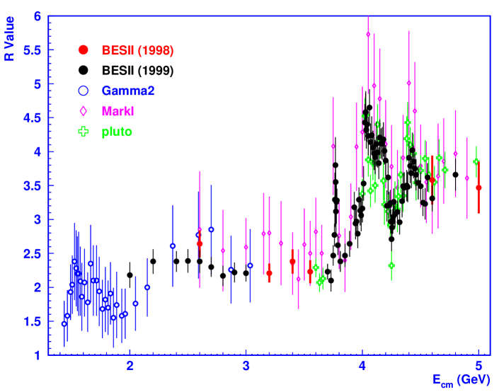
Figure 2: Values of $R$ measured by the BES Collaboration.

3. Neutral pion decay. The $\pi^{0}$ decay rate is governed by a quark loop diagram in which two photons are radiated by the quarks in $\pi^{0}=(u\bar{u}-d\bar{d})/\sqrt{2}$. The predicted rate is

$$\Gamma(\pi^{0}\to\gamma\gamma)=\frac{S^{2}m_{\pi}^{3}}{8\pi f_{\pi}^{2}}\left(\frac{\alpha}{2\pi}\right)^{2}~{}~{}~{},$$ (3)

where $f_{\pi}=131$ MeV and $S=N_{c}(Q_{u}^{2}-Q_{d}^{2})=N_{c}/3$. The experimental rate is $7.8\pm 0.6$ eV, while Eq. (3) gives $7.6S^{2}$ eV, in accord with experiment if $S=1$ and $N_{c}=3$.

4. Triality. Quark composites appear only in multiples of three. Baryons are composed of $qqq$, while mesons are $q\bar{q}$ (with total quark number zero). This is compatible with our current understanding of QCD, in which only color-singlet states can appear in the spectrum. Thus, mesons $M$ and baryons $B$ are represented by

$$M=\frac{1}{\sqrt{3}}(q^{a}\bar{q}^{\prime}_{a})~{}~{},~{}~{}~{}B=\frac{1}{\sqrt{6}}(\epsilon_{abc}q^{a}{q^{\prime}}^{b}{q^{\prime\prime}}^{c})~{}~{}~{}.$$ (4)

Direct evidence for the quanta of QCD, the gluons, was first presented in 1979 on the basis of extra “jets” of particles produced in electron-positron annihilations to hadrons. Normally one sees two clusters of energy associated with the fragmentation of each quark in $e^{+}e^{-}\to q\bar{q}$ into hadrons. However, in some fraction of events an extra jet was seen, corresponding to the radiation of a gluon by one of the quarks.

The transformations which take one color of quark into another are those of the group SU(3). We shall often refer to this group as SU(3)_color to distinguish it from the SU(3)_flavor associated with the quarks $u$, $d$, and $s$.

1.3 Electroweak unification

The electromagnetic interaction is described in terms of photon exchange, for which the Born approximation leads to a matrix element behaving as $1/q^{2}$. Here $q$ is the four-momentum transfer, and $q^{2}$ is its invariant square. The quantum electrodynamics of photons and charged pointlike particles (such as electrons) initially encountered calculational problems in the form of divergent quantities, but these had been tamed by the late 1940s through the procedure known as renormalization, leading to successful estimates of such quantities as the anomalous magnetic moment of the electron and the Lamb shift in hydrogen.

By contrast, the weak interactions as formulated up to the mid-1960s involved the pointlike interactions of two currents, with an interaction Hamiltonian ${\cal H}_{W}=G_{F}J_{\mu}J^{\mu{\dagger}}/\sqrt{2}$, with $G_{F}=1.16637(1)\times 10^{-5}$ GeV^-2 the current value for the Fermi coupling constant. This interaction is very singular and cannot be renormalized. The weak currents $J_{\mu}$ in this theory were purely charge-changing. As a result of work by Lee and Yang, Feynman and Gell-Mann, and Marshak and Sudarshan in 1956–7 they were identified as having (vector)–(axial) or “$V-A$” form.

Hideki Yukawa (1935) and Oskar Klein (1938) proposed a boson-exchange model for the charge-changing weak interactions. Klein’s model attempted a unification with electromagnetism and was based on a local isotopic gauge symmetry, thus anticipating the theory of Yang and Mills (1954). Julian Schwinger and others studied such models in the 1950s, but Glashow (1961) was the first to realize that a new neutral heavy boson had to be introduced as well in order to successfully unify the weak and electromagnetic interactions. The breaking of the electroweak symmetry (Weinberg 1967, Salam 1968) via the Higgs (1964) mechanism converted this phenomenological theory into one which could be used for higher-order calculations, as was shown by ’t Hooft and Veltman in the early 1970s.

The boson-exchange model for charge-changing interactions replaces the Fermi interaction constant with a coupling constant $g$ at each vertex and the low-$q^{2}$ limit of a propagator, $1/(M_{W}^{2}-q^{2})\to 1/M_{W}^{2}$, with factors of 2 chosen so that $G_{F}/\sqrt{2}=g^{2}/8M_{W}^{2}$. The $q^{2}$ term in the propagator helps the theory to be more convergent, but it is not the only ingredient needed, as we shall see.

The normalization of the charge-changing weak currents $J_{\mu}$ suggested well in advance of electroweak unification that one regard the corresponding integrals of their time components (the so-called weak charges) as members of an SU(2) algebra (Gell-Mann and Lévy 1960, Cabibbo 1963). However, the identification of the neutral member of this multiplet as the electric charge was problematic. In the $V-A$ theory the $W$’s couple only to left-handed fermions $\psi_{L}\equiv(1-\gamma_{5})\psi/2$, while the photon couples to $\psi_{L}+\psi_{R}$, where $\psi_{R}\equiv(1+\gamma_{5})\psi/2$. Furthermore, the high-energy behavior of the $\nu\bar{\nu}\to W^{+}W^{-}$ scattering amplitude based on charged lepton exchange leads to unacceptable divergences if we incorporate it into the one-loop contribution to $\nu\bar{\nu}\to\nu\bar{\nu}$ (Quigg 1983).

A simple solution was to add a neutral boson $Z$ coupling to $W^{+}W^{-}$ and $\nu\bar{\nu}$ in such a way as to cancel the leading high-energy behavior of the charged-lepton-exchange diagram. This relation between couplings occurs naturally in a theory based on the gauge group SU(2) $\otimes$ U(1). The $Z$ leads to neutral current interactions, in which (for example) an incident neutrino scatters inelastically on a hadronic target without changing its charge. The discovery of neutral-current interactions of neutrinos and many other manifestations of the $Z$ proved to be striking confirmations of the new theory.

If one identifies the $W^{+}$ and $W^{-}$ with raising and lowering operations in an SU(2), so that $W^{\pm}=(W^{1}\mp iW^{2})\sqrt{2}$, then left-handed fermions may be assigned to doublets of this “weak isospin,” with $I_{3L}(u,c,t)=I_{3L}(\nu_{e},\nu_{\mu},\nu_{\tau})=+1/2$, $I_{3L}(d,s,b)=I_{3L}(e^{-},\mu^{-},\tau^{-})=-1/2$. All the right-handed fermions have $I_{L}=I_{3L}=0$. As mentioned, one cannot simply identify the photon with $W^{3}$, which also couples only to left-handed fermions. Instead, one must introduce another boson $B$ associated with a U(1) gauge group. It will mix with the $W^{3}$ to form physical states consisting of the massless photon $A$ and the massive neutral boson $Z$:

$$A=B\cos\theta+W^{3}\sin\theta~{}~{},~{}~{}~{}Z=-B\sin\theta+W^{3}\cos\theta~{}~{}~{}.$$ (5)

The mixing angle $\theta$ appears in many electroweak processes. It has been measured to sufficiently great precision that one must specify the renormalization scheme in which it is quoted. For present purposes we shall merely note that $\sin^{2}\theta\simeq 0.23$. The corresponding SU(2) and U(1) coupling constants $g$ and $g^{\prime}$ are related to the electric charge $e$ by $e=g\sin\theta=g^{\prime}\cos\theta$, so that

$$\frac{1}{e^{2}}=\frac{1}{g^{2}}+\frac{1}{{g^{\prime}}^{2}}~{}~{}~{}.$$ (6)

The electroweak theory successfully predicted the masses of the $W^{\pm}$ and $Z$:

$$M_{W}\simeq 38.6{\rm~{}GeV}/\sin\theta\simeq 80.5{\rm~{}GeV}~{}~{},~{}~{}~{}M_{Z}\simeq M_{W}/\cos\theta\simeq 91.2{\rm~{}GeV}~{}~{}~{},$$ (7)

where we show the approximate experimental values. The detailed check of these predictions has reached the precision that one can begin to look into the deeper structure of the theory. A key ingredient in this structure is the Higgs boson, the price that had to be paid for the breaking of the electroweak symmetry.

1.4 Higgs boson

An unbroken SU(2) $\otimes$ U(1) theory involving the photon would require all fields to have zero mass, whereas the $W^{\pm}$ and $Z$ are massive. The symmetry-breaking which generates $W$ and $Z$ masses must not destroy the renormalizability of the theory. However, a massive vector boson propagator is of the form

$$D_{\mu\nu}(q)=\frac{-g_{\mu\nu}+q_{\mu}q_{\nu}/M^{2}}{q^{2}-M^{2}}$$ (8)

where $M$ is the boson mass. The terms $q_{\mu}q_{\nu}$, when appearing in loop diagrams, will destroy the renormalizability of the theory. They are associated with longitudinal vector boson polarizations, which are only present for massive bosons. For massless bosons like the photon, there are only transverse polarization states $J_{z}=\pm J$.

The Higgs mechanism, to be discussed in detail later in these lectures, provides the degrees of freedom needed to add a longitudinal polarization state for each of $W^{+}$, $W^{-}$, and $W^{0}$. In the simplest model, this is achieved by introducing a doublet of complex Higgs fields:

$$\phi=\left[\begin{array}[]{c}\phi^{+}\\ \phi^{0}\end{array}\right]~{}~{},~{}~{}~{}\phi^{*}=\left[\begin{array}[]{c}\bar{\phi}^{0}\\ \phi^{-}\end{array}\right]~{}~{}~{}.$$ (9)

Here the charged Higgs fields $\phi^{\pm}$ provide the longitudinal component of $W^{\pm}$ and the linear combination $(\phi^{0}-\bar{\phi}^{0})/i\sqrt{2}$ provides the longitudinal component of the $Z$. The additional degree of freedom $(\phi^{0}+\bar{\phi}^{0})/\sqrt{2}$ corresponds to a physical particle, the Higgs particle, which is the subject of intense searches.

Discovering the nature of the Higgs boson is a key to further progress in understanding what may lie beyond the Standard Model. There may exist one Higgs boson or more than one. There may exist other particles in the spectrum related to it. The Higgs boson may be elementary or composite. If composite, it points to a new level of substructure of the elementary particles. Much of our discussion will lead up to strategies for the next few years designed to address these questions. First, we introduce the necessary topic of gauge theories, which have been the platform for all the developments of the past thirty years.

2 Gauge theories

2.1 Abelian gauge theories

The Lagrangian describing a free fermion of mass $m$ is ${\cal L}_{\rm free}=\overline{\psi}(i\not\!\partial-m)\psi$. It is invariant under the global phase change $\psi\to\exp(i\alpha)\psi$. (We shall always consider the fermion fields to depend on $x$.) Now consider independent phase changes at each point:

$$\psi\to\psi^{\prime}\equiv\exp[i\alpha(x)]\psi.$$ (10)

Because of the derivative, the Lagrangian then acquires an additional phase change at each point: $\delta{\cal L}_{\rm free}=\overline{\psi}i\gamma^{\mu}[i\partial_{\mu}\alpha(x)]\psi$. The free Lagrangian is not invariant under such changes of phase, known as local gauge transformations.

Local gauge invariance can be restored if we make the replacement $\partial_{\mu}\to D_{\mu}\equiv\partial_{\mu}+ieA_{\mu}$ in the free-fermion Lagrangian, which now is

$${\cal L}=\overline{\psi}(i\not\!\!D-m)\psi=\overline{\psi}(i\not\!\partial-m)\psi-e\overline{\psi}\not\!\!A(x)\psi~{}~{}~{}.$$ (11)

The effect of a local phase in $\psi$ can be compensated if we allow the vector potential $A_{\mu}$ to change by a total divergence, which does not change the electromagnetic field strength (defined as in Peskin and Schroeder 1995; Quigg 1983 uses the opposite sign)

$$F_{\mu\nu}\equiv\partial_{\mu}A_{\nu}-\partial_{\nu}A_{\nu}~{}~{}~{}.$$ (12)

Indeed, under the transformation $\psi\to\psi^{\prime}$ and with $A\to A^{\prime}$ with $A^{\prime}$ yet to be determined, we have

$${\cal L}^{\prime}=\overline{\psi}^{\prime}(i\not\!\partial-m)\psi^{\prime}-e\overline{\psi}^{\prime}{\not\!\!A}^{\prime}\psi^{\prime}=\overline{\psi}(i\not\!\partial-m)\psi-\overline{\psi}[\not\!\partial\alpha(x)]\psi-e\overline{\psi}{\not\!\!A}^{\prime}\psi~{}~{}~{}.$$ (13)

This will be the same as ${\cal L}$ if

$$A^{\prime}_{\mu}(x)=A_{\mu}(x)-\frac{1}{e}\partial_{\mu}\alpha(x)~{}~{}~{}.$$ (14)

The derivative $D_{\mu}$ is known as the covariant derivative. One can check that under a local gauge transformation, $D_{\mu}\psi\to e^{i\alpha(x)}D_{\mu}\psi$.

Another way to see the consequences of local gauge invariance suggested by Yang (1974) and discussed by Peskin and Schroeder (1995, pp 482–486) is to define $-eA_{\mu}(x)$ as the local change in phase undergone by a particle of charge $e$ as it passes along an infinitesimal space-time increment between $x^{\mu}$ and $x^{\mu}+dx^{\mu}$. For a space-time trip from point $A$ to point $B$, the phase change is then

$$\Phi_{AB}=\exp\left(-ie\int_{A}^{B}A_{\mu}(x)dx^{\mu}\right)~{}~{}~{}.$$ (15)

The phase in general will depend on the path in space-time taken from point $A$ to point $B$. As a consequence, the phase $\Phi_{AB}$ is not uniquely defined. However, one can compare the result of a space-time trip along one path, leading to a phase $\Phi_{AB}^{(1)}$, with that along another, leading to a phase $\Phi_{AB}^{(2)}$. The two-slit experiment in quantum mechanics involves such a comparison; so does the Bohm-Aharonov effect in which a particle beam traveling past a solenoid on one side interferes with a beam traveling on the other side. Thus, phase differences

$$\Phi_{AB}^{(1)}\Phi_{AB}^{(2)*}=\Phi_{C}=\exp\left(-ie\oint A_{\mu}(x)dx^{\mu}\right)~{}~{}~{},$$ (16)

associated with closed paths in space-time (represented by the circle around the integral sign), are the ones which correspond to physical experiments. The phase $\Phi_{C}$ for a closed path $C$ is independent of the phase convention for a charged particle at any space-time point $x_{0}$, since any change in the contribution to $\Phi_{C}$ from the integral up to $x_{0}$ will be compensated by an equal and opposite contribution from the integral departing from $x_{0}$.

The closed path integral (16) can be expressed as a surface integral using Stokes’ theorem:

$$\oint A_{\mu}(x)dx^{\mu}=\int F_{\mu\nu}(x)d\sigma^{\mu\nu}~{}~{}~{},$$ (17)

where the electromagnetic field strength $F_{\mu\nu}$ was defined previously and $d\sigma^{\mu\nu}$ is an element of surface area. It is also clear that the closed path integral is invariant under changes (14) of $A_{\mu}(x)$ by a total divergence. Thus $F_{\mu\nu}$ suffices to describe all physical experiments as long as one integrates over a suitable domain. In the Bohm-Aharonov effect, in which a charged particle passes on either side of a solenoid, the surface integral will include the solenoid (in which the magnetic field is non-zero).

If one wishes to describe the energy and momentum of free electromagnetic fields, one must include a kinetic term ${{\cal L}}_{K}=-(1/4)F_{\mu\nu}F^{\mu\nu}$ in the Lagrangian, which now reads

$${\cal L}=-\frac{1}{4}F_{\mu\nu}F^{\mu\nu}+\overline{\psi}(i\not\!\partial-m)\psi-e\overline{\psi}\not\!\!A\psi~{}~{}~{}.$$ (18)

If the electromagnetic current is defined as $J^{\rm em}_{\mu}\equiv\overline{\psi}\gamma_{\mu}\psi$, this Lagrangian leads to Maxwell’s equations.

The local phase changes (10) form a U(1) group of transformations. Since such transformations commute with one another, the group is said to be Abelian. Electrodynamics, just constructed here, is an example of an Abelian gauge theory.

2.2 Non-Abelian gauge theories

One can imagine that a particle traveling in space-time undergoes not only phase changes, but also changes of identity. Such transformations were first considered by Yang and Mills (1954). For example, a quark can change in color (red to blue) or flavor ($u$ to $d$). In that case we replace the coefficient $eA_{\mu}$ of the infinitesimal displacement $dx_{\mu}$ by an $n\times n$ matrix $-g{\bf A}_{\mu}(x)\equiv-gA^{i}_{\mu}(x){\bf T}_{i}$ acting in the $n$-dimensional space of the particle’s degrees of freedom. (The sign change follows the convention of Peskin and Schroeder 1995.) For colors, $n=3$. The ${\bf T}_{i}$ form a linearly independent basis set of matrices for such transformations, while the $A^{i}_{\mu}$ are their coefficients. The phase transformation then must take account of the fact that the matrices ${\bf A}_{\mu}(x)$ in general do not commute with one another for different space-time points, so that a path-ordering is needed:

$$\Phi_{AB}={\cal P}\left[\exp\left(ig\int_{A}^{B}{\bf A}_{\mu}(x)dx^{\mu}\right)\right]~{}~{}~{}.$$ (19)

When the basis matrices ${\bf T}_{i}$ do not commute with one another, the theory is non-Abelian.

We demand that changes in phase or identity conserve probability, i.e., that $\Phi_{AB}$ be unitary: $\Phi^{\dagger}_{AB}\Phi_{AB}=1$. When $\Phi_{AB}$ is a matrix, the corresponding matrices ${\bf A}_{\mu}(x)$ in (19) must be Hermitian. If we wish to separate out pure phase changes, in which ${\bf A}_{\mu}(x)$ is a multiple of the unit matrix, from the remaining transformations, one may consider only transformations such that det$(\Phi_{AB})=1$, corresponding to traceless ${\bf A}_{\mu}(x)$.

The $n\times n$ basis matrices ${\bf T}_{i}$ must then be Hermitian and traceless. There will be $n^{2}-1$ of them, corresponding to the number of independent SU(N) generators. (One can generalize this approach to other invariance groups.) The matrices will satisfy the commutation relations

$$[{\bf T}_{i},{\bf T}_{j}]=ic_{ijk}{\bf T}_{k}~{}~{}~{},$$ (20)

where the $c_{ijk}$ are structure constants characterizing the group. For SU(2), $c_{ijk}=\epsilon_{ijk}$ (the Kronecker symbol), while for SU(3), $c_{ijk}=f_{ijk}$, where the $f_{ijk}$ are defined in Gell-Mann and Ne’eman (1964). A $3\times 3$ representation in SU(3) is ${\bf T}_{i}=\lambda_{i}/2$, where $\lambda_{i}/2$ are the Gell-Mann matrices normalized such that Tr $\lambda_{i}\lambda_{j}=2\delta_{ij}$. For this representation, then, Tr ${\bf T}_{i}{\bf T}_{j}=\delta_{ij}/2$.

In order to define the field-strength tensor ${\bf F}_{\mu\nu}=F^{i}_{\mu\nu}{\bf T}_{i}$ for a non-Abelian transformation, we may consider an infinitesimal closed-path transformation analogous to Eq. (16) for the case in which the matrices ${\bf A}_{\mu}(x)$ do not commute with one another. The result (see, e.g., Peskin and Schroeder 1995, pp 486–491) is

$${\bf F}_{\mu\nu}=\partial_{\mu}{\bf A}_{\nu}-\partial_{\nu}{\bf A}_{\nu}-ig[{\bf A}_{\mu},{\bf A}_{\nu}]~{}~{},~{}~{}~{}F^{i}_{\mu\nu}=\partial_{\mu}A^{i}_{\nu}-\partial_{\nu}A^{i}_{\mu}+gc_{ijk}A^{j}_{\mu}A^{k}_{\nu}~{}~{}~{}.$$ (21)

An alternative way to introduce non-Abelian gauge fields is to demand that, by analogy with Eq. (10), a theory involving fermions $\psi$ be invariant under local transformations

$$\psi(x)\to\psi^{\prime}(x)=U(x)\psi(x)~{}~{},~{}~{}~{}U^{\dagger}U=1~{}~{}~{},$$ (22)

where for simplicity we consider unitary transformations. Under this replacement, ${\cal L}\to{\cal L}^{\prime}$, where

$${\cal L}^{\prime}\equiv\overline{\psi}^{\prime}(i\not\!\partial-m)\psi^{\prime}=\overline{\psi}U^{-1}(i\not\!\partial-m)U\psi$$

$$=\overline{\psi}(i\not\!\partial-m)\psi+i\psi U^{-1}\gamma^{\mu}(\partial_{\mu}U)\psi~{}~{}~{}.$$ (23)

As in the Abelian case, an extra term is generated by the local transformation. It can be compensated by replacing $\partial_{\mu}$ by

$$\partial_{\mu}\to{\bf D}_{\mu}\equiv\partial_{\mu}-ig{\bf A}_{\mu}(x)~{}~{}~{}.$$ (24)

In this case ${\cal L}=\overline{\psi}(i\not\!\!{\bf D}-m)\psi$ and under the change (22) we find

$${\cal L}^{\prime}\equiv\overline{\psi}^{\prime}(i\not\!\!{\bf D}^{\prime}-m)\psi^{\prime}=\overline{\psi}U^{-1}(i\not\!\partial+g\not\!\!{\bf A}^{\prime}-m)U\psi$$

$$={\cal L}+\overline{\psi}[g(U^{-1}\not\!\!{\bf A}^{\prime}U-\not\!\!{\bf A})+iU^{-1}(\not\!\partial U)]\psi~{}~{}~{}.$$ (25)

This is equal to ${\cal L}$ if we take

$${\bf A}_{\mu}^{\prime}=U{\bf A}_{\mu}U^{-1}-\frac{i}{g}(\partial_{\mu}U)U^{-1}~{}~{}~{}.$$ (26)

This reduces to our previous expressions if $g=-e$ and $U=e^{i\alpha(x)}$.

The covariant derivative acting on $\psi$ transforms in the same way as $\psi$ itself under a gauge transformation: ${\bf D}_{\mu}\psi\to{\bf D}_{\mu}^{\prime}\psi^{\prime}=U{\bf D}_{\mu}\psi$. The field strength ${\bf F}_{\mu\nu}$ transforms as ${\bf F}_{\mu\nu}\to{\bf F}_{\mu\nu}^{\prime}=U{\bf F}_{\mu\nu}U^{-1}$. It may be computed via $[{\bf D}_{\mu},{\bf D}_{\nu}]=-ig{\bf F}_{\mu\nu}$; both sides transform as $U(~{}~{})U^{-1}$ under a local gauge transformation.

In order to obtain propagating gauge fields, as in electrodynamics, one must add a kinetic term ${{\cal L}}_{K}=-(1/4)F^{i}_{\mu\nu}F^{i\mu\nu}$ to the Lagrangian. Recalling the representation ${\bf F}_{\mu\nu}=F^{i}_{\mu\nu}$ in terms of gauge group generators normalized such that Tr$({\bf T}_{i}{\bf T}_{j})=\delta_{ij}/2$, we can write the full Yang-Mills Lagrangian for gauge fields interacting with matter fields as

$${\cal L}=-\frac{1}{2}{\rm Tr}({\bf F}_{\mu\nu}{\bf F}^{\mu\nu})+\overline{\psi}(i\not\!\!{\bf D}-m)\psi~{}~{}~{}.$$ (27)

We shall use Lagrangians of this type to derive the strong, weak, and electromagnetic interactions of the “Standard Model.”

The interaction of a gauge field with fermions then corresponds to a term in the interaction Lagrangian $\Delta{\cal L}=g\overline{\psi}(x)\gamma^{\mu}{\bf A}_{\mu}(x)\psi(x)$. The $[{\bf A}_{\mu},{\bf A}_{\nu}]$ term in ${\bf F}_{\mu\nu}$ leads to self-interactions of non-Abelian gauge fields, arising solely from the kinetic term. Thus, one has three- and four-field vertices arising from

$$\Delta{{\cal L}}_{K}^{(3)}=(\partial_{\mu}A^{i}_{\nu})gc_{ijk}A^{\mu j}A^{\nu k}~{}~{},~{}~{}~{}\Delta{{\cal L}}_{K}^{(4)}=-\frac{g^{2}}{4}c_{ijk}c_{imn}A^{\mu j}A^{\nu k}A^{m}_{\mu}A^{n}_{\nu}~{}~{}~{}.$$ (28)

These self-interactions are an important aspect of non-Abelian gauge theories and are responsible in particular for the remarkable asymptotic freedom of QCD which leads to its becoming weaker at short distances, permitting the application of perturbation theory.

2.3 Elementary divergent quantities

In most quantum field theories, including quantum electrodynamics, divergences occurring in higher orders of perturbation theory must be removed using charge, mass, and wave function renormalization. This is conventionally done at intermediate calculational stages by introducing a cutoff momentum scale $\Lambda$ or analytically continuing the number of space-time dimensions away from four. Thus, a vacuum polarization graph in QED associated with external photon momentum $k$ and a fermion loop will involve an integral

$$\Pi_{\mu\nu}(k)\sim\int\frac{d^{4}p}{(2\pi)^{4}}{\rm Tr}\left(\frac{1}{\not\!p-m}\gamma_{\mu}\frac{1}{\not\!p+\not\!k-m}\gamma_{\nu}\right)~{}~{}~{};$$ (29)

a self-energy of a fermion with external momentum $p$ will involve

$$\Sigma(p)\sim\int\frac{d^{4}q}{(2\pi)^{4}}\frac{1}{q^{2}}\gamma_{\mu}\frac{1}{\not\!p+\not\!q-m}\gamma^{\mu}~{}~{}~{},$$ (30)

and a fermion-photon vertex function with external fermion momenta $p,p^{\prime}$ will involve

$$\Lambda_{\mu}(p^{\prime},p)\sim\int\frac{d^{4}k}{(2\pi)^{4}}\frac{1}{k^{2}}\gamma_{\nu}\frac{1}{\not\!p^{\prime}+\not\!k-m}\gamma_{\mu}\frac{1}{\not\!p+\not\!k-m}\gamma^{\nu}~{}~{}~{}.$$ (31)

The integral (29) appears to be quadratically divergent. However, the gauge invariance of the theory translates into the requirement $k^{\mu}\Pi_{\mu\nu}=0$, which requires $\Pi_{\mu\nu}$ to have the form

$$\Pi_{\mu\nu}(k)=(k^{2}g_{\mu\nu}-k_{\mu}k_{\nu})\Pi(k^{2})~{}~{}~{}.$$ (32)

The corresponding integral for $\Pi(k^{2})$ then will be only logarithmically divergent. The integral in (30) is superficially linearly divergent but in fact its divergence is only logarithmic, as is the integral in (31).

Unrenormalized functions describing vertices and self-energies involving $n_{B}$ external boson lines and $n_{F}$ external fermion lines may be defined in terms of a momentum cutoff $\Lambda$ and a bare coupling constant $g_{0}$ (Coleman 1971, Ellis 1977, Ross 1978):

$$\Gamma^{U}_{n_{B},n_{F}}\equiv\Gamma^{U}_{n_{B},n_{F}}(p_{i},g_{0},\Lambda)~{}~{},$$ (33)

where $p_{i}$ denote external momenta. Renormalized functions $\Gamma^{R}$ may be defined in terms of a scale parameter $\mu$, a renormalized coupling constant $g=g(g_{0},\Lambda/\mu)$, and renormalization constants $Z_{B}(\Lambda)$ and $Z_{F}(\Lambda)$ for the external boson and fermion wave functions:

$$\Gamma^{R}(p_{i},g,\mu)\equiv\lim_{\Lambda\to\infty}[Z_{B}(\Lambda)]^{n_{B}}[Z_{F}(\Lambda)]^{n_{F}}\Gamma^{U}_{n_{B},n_{F}}(p_{i},g_{0},\Lambda)~{}~{}~{}.$$ (34)

The scale $\mu$ is typically utilized by demanding that $\Gamma^{R}$ be equal to some predetermined function at a Euclidean momentum $p^{2}=-\mu^{2}$. Thus, for the one-boson, two-fermion vertex, we take

$$\Gamma^{R}_{1,2}(0,p,-p)|_{p^{2}=-\mu^{2}}=\lim_{\Lambda\to\infty}Z_{F}^{2}Z_{B}\Gamma^{U}_{1,2}(0,p,-p)|_{p^{2}=-\mu^{2}}\equiv g~{}~{}~{}.$$ (35)

The unrenormalized function $\Gamma^{U}$ is independent of $\mu$, while $\Gamma^{R}$ and the renormalization constants $Z_{B}(\Lambda),~{}Z_{F}(\Lambda)$ will depend on $\mu$. For example, in QED, the photon wave function renormalization constant (known as $Z_{3}$) behaves as

$$Z_{3}=1-\frac{\alpha_{0}}{3\pi}\ln\frac{\Lambda^{2}}{\mu^{2}}~{}~{}~{}.$$ (36)

The bare charge $e_{0}$ and renormalized charge $e$ are related by $e=e_{0}Z_{3}^{1/2}$. To lowest order in perturbation theory, $e<e_{0}$. The vacuum behaves as a normal dielectric; charge is screened. It is the exception rather than the rule that in QED one can define the renormalized charge for $q^{2}=0$; in QCD we shall see that this is not possible.

2.4 Scale changes and the beta function

We differentiate both sides of (34) with respect to $\mu$ and multiply by $\mu$. Since the functions $\Gamma^{U}$ are independent of $\mu$, we find

$$\left(\mu\frac{\partial}{\partial\mu}+\mu\frac{\partial g}{\partial\mu}\frac{\partial}{\partial g}\right)\Gamma^{R}(p_{i},g,\mu)$$

$$=\lim_{\Lambda\to\infty}\left(\frac{n_{B}}{Z_{B}}\mu\frac{\partial Z_{B}}{\partial\mu}+\frac{n_{F}}{Z_{F}}\mu\frac{\partial Z_{F}}{\partial\mu}\right)Z_{B}^{n_{B}}Z_{F}^{n_{F}}\Gamma^{U}~{}~{}~{},$$ (37)

or

$$\left[\mu\frac{\partial}{\partial\mu}+\beta(g)\frac{\partial}{\partial g}+n_{B}\gamma_{B}(g)+n_{F}\gamma_{F}(g)\right]\Gamma^{R}(p_{i},g,\mu)=0~{}~{}~{},$$ (38)

where

$$\beta(g)\equiv\mu\frac{\partial g}{\partial\mu}~{}~{},~{}~{}~{}\gamma_{B}(g)\equiv-\frac{\mu}{Z_{B}}\frac{\partial Z_{B}}{\partial\mu}~{}~{},~{}~{}~{}\gamma_{F}(g)\equiv-\frac{\mu}{Z_{F}}\frac{\partial Z_{F}}{\partial\mu}~{}~{}~{}.$$ (39)

The behavior of any generalized vertex function $\Gamma^{R}$ under a change of scale $\mu$ is then governed by the universal functions (39).

Here we shall be particularly concerned with the function $\beta(g)$. Let us imagine $\mu\to\lambda\mu$ and introduce the variables $t\equiv\ln\lambda$, $\bar{g}(g,t)\equiv g(g_{0},\Lambda/\lambda\mu)$, Then the relation for the beta-function may be written

$$\frac{d\bar{g}(g,t)}{dt}=\beta(\bar{g})~{}~{},~{}~{}~{}\bar{g}(g,0)=g(g_{0},\Lambda/\mu)=g~{}~{}~{}.$$ (40)

Let us compare the behavior of $\bar{g}$ with increasing $t$ (larger momentum scales or shorter distance scales) depending on the sign of $\beta(\bar{g})$. In general we will find $\beta(0)=0$. We take $\beta(\bar{g})$ to have zeroes at $\bar{g}=0,~{}g_{1},~{}g_{2},~{}\ldots$. Then:

1. Suppose $\beta(\bar{g})>0$. Then $\bar{g}$ increases from its $t=0$ value $\bar{g}=g$ until a zero $g_{i}$ of $\beta(\bar{g})$ is encountered. Then $\bar{g}\to g_{i}$ as $t\to\infty$.

2. Suppose $\beta(\bar{g})<0$. Then $\bar{g}$ decreases from its $t=0$ value $\bar{g}=g$ until a zero $g_{i}$ of $\beta(\bar{g})$ is encountered.

In either case $\bar{g}$ approaches a point at which $\beta(\bar{g})=0$, $\beta^{\prime}(\bar{g})<0$ as $t\to\infty$. Such points are called ultraviolet fixed points. Similarly, points for which $\beta(\bar{g})=0$, $\beta^{\prime}(\bar{g})>0$ are infrared fixed points, and $\bar{g}$ will tend to them for $t\to-\infty$ (small momenta or large distances). The point $e=0$ is an infrared fixed point for quantum electrodynamics, since $\beta^{\prime}(e)>0$ at $e=0$.

It may happen that $\beta^{\prime}(0)<0$ for specific theories. In that case $\bar{g}=0$ is an ultraviolet fixed point, and the theory is said to be asymptotically free. We shall see that this property is particular to non-Abelian gauge theories (Gross and Wilczek 1973, Politzer 1974).

2.5 Beta function calculation

In quantum electrodynamics a loop diagram involving a fermion of unit charge contributes the following expression to the relation between the bare charge $e_{0}$ and the renormalized charge $e$:

$$e=e_{0}\left(1-\frac{\alpha_{0}}{3\pi}\ln\frac{\Lambda}{\mu}\right)~{}~{}~{},$$ (41)

as implied by (35) and (36), where $\alpha_{0}\equiv e_{0}^{2}/4\pi$. We find

$$\beta(e)=\frac{e_{0}^{3}}{12\pi^{2}}\simeq\frac{e^{3}}{12\pi^{2}}~{}~{}~{},$$ (42)

where differences between $e_{0}$ and $e$ correspond to higher-order terms in $e$. (Here $\alpha\equiv e^{2}/4\pi$.) Thus $\beta(e)>0$ for small $e$ and the coupling constant becomes stronger at larger momentum scales (shorter distances).

We shall show an extremely simple way to calculate (42) and the corresponding result for a charged scalar particle in a loop. From this we shall be able to first calculate the effect of a charged vector particle in a loop (a calculation first performed by Khriplovich 1969) and then generalize the result to Yang-Mills fields. The method follows that of Hughes (1980).

When one takes account of vacuum polarization, the electromagnetic interaction in momentum space may be written

$$\frac{e^{2}}{q^{2}}\to\frac{e^{2}}{q^{2}[1+\Pi(q^{2})]}~{}~{}~{}$$ (43)

Here the long-distance ($q^{2}\to 0$) behavior has been defined such that $e$ is the charge measured at macroscopic distances, so $\Pi(0)=0$. Following Sakurai (1967), we shall reconstruct $\Pi_{i}(q^{2})$ for a loop involving the fermion species $i$ from its imaginary part, which is measurable through the cross section for $e^{+}e^{-}\to i\bar{i}$:

$${\rm Im}~{}\Pi_{i}(s)=\frac{s}{4\pi\alpha}\sigma(e^{+}e^{-}\to i\bar{i})~{}~{}~{},$$ (44)

where $s$ is the square of the center-of-mass energy. For fermions $f$ of charge $e_{f}$ and mass $m_{f}$,

$${\rm Im}~{}\Pi_{f}(s)=\frac{\alpha e_{f}^{2}}{3}\left(1+\frac{2m_{f}^{2}}{s}\right)\left(1-\frac{4m_{f}^{2}}{s}\right)^{1/2}\theta(s-4m_{f}^{2})~{}~{}~{},$$ (45)

while for scalar particles of charge $e_{s}$ and mass $m_{s}$,

$${\rm Im}~{}\Pi_{s}(s)=\frac{\alpha e_{s}^{2}}{12}\left(1-\frac{4m_{s}^{2}}{s}\right)^{3/2}\theta(s-4m_{s}^{2})~{}~{}~{}.$$ (46)

The corresponding cross section for $e^{+}e^{-}\to\mu^{+}\mu^{-}$, neglecting the muon mass, is $\sigma(e^{+}e^{-}\to\mu^{+}\mu^{-})=4\pi\alpha^{2}/3s$, so one can define

$$R_{i}\equiv\sigma(e^{+}e^{-}\to i\bar{i})/\sigma(e^{+}e^{-}\to\mu^{+}\mu^{-})~{}~{}~{},$$ (47)

in terms of which Im $\Pi_{i}(s)=\alpha R_{i}(s)/3$. For $s\to\infty$ one has $R_{f}(s)\to e_{f}^{2}$ for a fermion and $R_{s}(s)\to e_{s}^{2}/4$ for a scalar.

The full vacuum polarization function $\Pi_{i}(s)$ cannot directly be reconstructed in terms of its imaginary part via the dispersion relation

$$\Pi_{i}(s)=\frac{1}{\pi}\int_{4m^{2}}^{\infty}\frac{ds^{\prime}}{s^{\prime}-s}{\rm Im}~{}\Pi_{i}(s^{\prime})~{}~{}~{},$$ (48)

since the integral is logarithmically divergent. This divergence is exactly that encountered earlier in the discussion of renormalization. For quantum electrodynamics we could deal with it by defining the charge at $q^{2}=0$ and hence taking $\Pi_{i}(0)=0$. The once-subtracted dispersion relation for $\Pi_{i}(s)-\Pi_{i}(0)$ would then converge:

$$\Pi_{i}(s)=\frac{1}{\pi}\int_{4m^{2}}^{\infty}\frac{ds^{\prime}}{s^{\prime}(s^{\prime}-s)}{\rm Im}~{}\Pi_{i}(s^{\prime})~{}~{}~{}.$$ (49)

However, in order to be able to consider cases such as Yang-Mills fields in which the theory is not well-behaved at $q^{2}=0$, let us instead define $\Pi_{i}(-\mu^{2})=0$ at some spacelike scale $q^{2}=-\mu^{2}$. The dispersion relation is then

$$\Pi_{i}(s)=\frac{1}{\pi}\int_{4m^{2}}^{\infty}ds^{\prime}\left[\frac{1}{s^{\prime}-s}-\frac{1}{s^{\prime}+\mu^{2}}\right]{\rm Im}~{}\Pi_{i}(s^{\prime})~{}~{}~{}.$$ (50)

For $|q^{2}|\gg\mu^{2}\gg m^{2}$, we find

$$\Pi_{i}(q^{2})\to-\frac{\alpha}{3\pi}R_{i}(\infty)\left[\ln\frac{-q^{2}}{\mu^{2}}+{\rm const.}\right]~{}~{}~{},$$ (51)

and so, from (43), the “charge at scale $q$” may be written as

$$e_{q}^{2}\equiv\frac{e^{2}}{1+\Pi_{i}(q^{2})}\simeq e^{2}\left[1+\frac{\alpha}{3\pi}R_{i}(\infty)\ln\frac{-q^{2}}{\mu^{2}}\right]~{}~{}~{}.$$ (52)

The beta-function here is defined by $\beta(e)=\mu(\partial e/\partial\mu)|_{{\rm fixed}~{}e_{q}}$. Thus, expressing $\beta(e)=-\beta_{0}e^{3}/(16\pi^{2})+{\cal O}(e^{5})$, one finds $\beta_{0}=-(4/3)e_{f}^{2}$ for spin-1/2 fermions and $\beta_{0}=-(1/3)e_{s}^{2}$ for scalars.

These results will now be used to find the value of $\beta_{0}$ for a single charged massless vector field. We generalize the results for spin 0 and 1/2 to higher spins by splitting contributions to vacuum polarization into “convective” and “magnetic” ones. Furthermore, we take into account the fact that a closed fermion loop corresponds to an extra minus sign in $\Pi_{f}(s)$ (which is already included in our result for spin 1/2). The “magnetic” contribution of a particle with spin projection $S_{z}$ must be proportional to $S_{z}^{2}$. For a massless spin-$S$ particle, $S_{z}^{2}=S^{2}$. We may then write

$$\beta_{0}=\left\{\begin{array}[]{c}(-1)^{n_{F}}(aS^{2}+b)(S=0)~{}~{}~{},\\ (-1)^{n_{F}}(aS^{2}+2b)(S\neq 0)~{}~{}~{},\end{array}\right.$$ (53)

where $n_{F}=1$ for a fermion, 0 for a boson. The factor of $2b$ for $S\neq 0$ comes from the contribution of each polarization state $(S_{z}=\pm S)$ to the convective term. Matching the results for spins 0 and 1/2,

$$-\frac{1}{3}=b~{}~{}~{},~{}~{}-\frac{4}{3}=-\left(\frac{a}{4}+2b\right)~{}~{}~{},$$ (54)

we find $a=8$ and hence for $S=1$

$$\beta_{0}=8-\frac{2}{3}=\frac{22}{3}~{}~{}~{}.$$ (55)

The magnetic contribution is by far the dominant one (by a factor of 12), and is of opposite sign to the convective one. A similar separation of contributions, though with different interpretations, was obtained in the original calculation of Khriplovich (1969). The reversal of sign with respect to the scalar and spin-1/2 results is notable.

2.6 Group-theoretic techniques

The result (55) for a charged, massless vector field interacting with the photon is also the value of $\beta_{0}$ for the Yang-Mills group SO(3) $\sim$ SU(2) if we identify the photon with $A^{3}_{\mu}$ and the charged vector particles with $A^{\pm}_{\mu}\equiv(A^{1}_{\mu}\mp iA^{2}_{\mu})/\sqrt{2}$. We now generalize it to the contribution of gauge fields in an arbitrary group $G$.

The value of $\beta_{0~{}{\rm gauge~{}fields}}$ depends on a sum over all possible self-interacting gauge fields that can contribute to the loop with external gauge field labels $i$ and $m$:

$$\frac{\beta_{0}[G]}{\beta_{0}[SU(2)]}=\frac{c^{G}_{ijk}c^{G}_{mjk}}{c^{\rm SU(2)}_{ijk}c^{\rm SU(2)}_{mjk}}~{}~{}~{},$$ (56)

where $c^{G}_{ijk}$ is the structure constant for $G$, introduced in Eq. (20). The sums in (56) are proportional to $\delta_{im}$:

$$c_{ijk}c_{mjk}=\delta_{im}C_{2}(A)~{}~{}~{}.$$ (57)

The quantity $C_{2}(A)$ is the quadratic Casimir operator for the adjoint representation of the group $G$.

Since the structure constants for SO(3) $\sim$ SU(2) are just $c^{\rm SU(2)}_{ijk}=\epsilon_{ijk}$, one finds $C_{2}(A)=2$ for SU(2), so the generalization of (55) is that $\beta_{0~{}{\rm gauge~{}fields}}=(11/3)C_{2}(A)$.

The contributions of arbitrary scalars and spin-1/2 fermions in representations $R$ are proportional to $T(R)$, where

$${\rm Tr}~{}(T_{i}T_{j})\equiv\delta_{ij}T(R)$$ (58)

for matrices $T_{i}$ in the representation $R$. For a single charged scalar particle (e.g., a pion) or fermion (e.g., an electron), $T(R)=1$. Thus $\beta_{0~{}{\rm spin~{}0}}=-(1/3)T_{0}(R)$, while $\beta_{0~{}{\rm spin~{}1/2}}=-(4/3)T_{1/2}(R)$, where the subscript on $T(R)$ denotes the spin. Summarizing the contributions of gauge bosons, spin 1/2 fermions, and scalars, we find

$$\beta_{0}=\frac{11}{3}C_{2}(A)-\frac{4}{3}\sum_{f}T_{1/2}(R_{f})-\sum_{s}\frac{1}{3}T_{0}(R_{s})~{}~{}~{}.$$ (59)

One often needs the beta-function to higher orders, notably in QCD where the perturbative expansion coefficient is not particularly small. It is

$$\beta(\bar{g})=-\beta_{0}\frac{\bar{g}^{3}}{16\pi^{2}}-\beta_{1}\frac{\bar{g}^{5}}{(16\pi^{2})^{2}}+\ldots~{}~{}~{},$$ (60)

where the result for gauge bosons and spin 1/2 fermions (Caswell 1974) is

$$\beta_{1}=\frac{2}{3}\left\{17[C_{2}(A)]^{2}-10T(R)C_{2}(A)-6T(R)C_{2}(R)\right\}~{}~{}~{}.$$ (61)

The first term involves loops exclusively of gauge bosons. The second involves single-gauge-boson loops with a fermion loop on one of the gauge boson lines. The third involves fermion loops with a fermion self-energy due to a gauge boson. The quantity $C_{2}(R)$ is defined such that

$$[T^{i}(R)T^{i}(R)]_{\alpha\beta}=C_{2}(R)\delta_{\alpha\beta}~{}~{}~{},$$ (62)

where $\alpha$ and $\beta$ are indices in the fermion representation.

We now illustrate the calculation of $C_{2}(A)$, $T(R)$, and $C_{2}(R)$ for SU(N). More general techniques are given by Slansky (1981).

Any SU(N) group contains an SU(2) subgroup, which we may take to be generated by $T_{1}$, $T_{2}$, and $T_{3}$. The isospin projection $I_{3}$ may be identified with $T_{3}$. Then the $I_{3}$ value carried by each generator $T_{i}$ (written for convenience in the fundamental N-dimensional representation) may be identified as shown below:

$\leftarrow 2\rightarrow$		$\leftarrow N-2\rightarrow$
0	1	1/2	$\cdots$	1/2
$-1$	0	$-1/2$	$\cdots$	$-1/2$
$-1/2$	1/2	0	$\cdots$	0
$\cdots$	$\cdots$	$\cdots$	$\cdots$	$\cdots$
$-1/2$	1/2	0	$\cdots$	0

Since $C_{2}(A)$ may be calculated for any convenient value of the index $i=m$ in (57), we chose $i=m=3$. Then

$$C_{2}(A)=\sum_{\rm adjoint}(I_{3})^{2}=1+1+4(N-2)\left(\frac{1}{2}\right)^{2}=N~{}~{}~{}.$$ (63)

As an example, the octet (adjoint) representation of SU(3) has two members with $|I_{3}|=1$ (e.g., the charged pions) and four with $|I_{3}|=1/2$ (e.g., the kaons).

For members of the fundamental representation of SU(N), there will be one member with $I_{3}=+1/2$, another with $I_{3}=-1/2$, and all the rest with $I_{3}=0$. Then again choosing $i=m=3$ in Eq. (58), we find $T(R)|_{\rm fundamental}=1/2$. The SU(N) result for $\beta_{0}$ in the presence of $n_{f}$ spin 1/2 fermions and $n_{s}$ scalars in the fundamental representation then may be written

$$\beta_{0}=\frac{11}{3}N-\frac{2}{3}n_{f}-\frac{1}{6}n_{s}~{}~{}~{}.$$ (64)

The quantity $C_{2}(A)$ in (63) is most easily calculated by averaging over all indices $\alpha=\beta$. If all generators $T^{i}$ are normalized in the same way, one may calculate the result for an individual generator (say, $T_{3}$) and then multiply by the number of generators [$N^{2}-1$ for SU(N)]. For the fundamental representation one then finds

$$C_{2}(R)=\frac{1}{N}(N^{2}-1)\left[\left(\frac{1}{2}\right)^{2}+\left(-\frac{1}{2}\right)^{2}\right]=\frac{N^{2}-1}{2N}~{}~{}~{}.$$ (65)

2.7 The running coupling constant

One may integrate Eq. (60) to obtain the coupling constant as a function of momentum scale $M$ and a scale-setting parameter $\Lambda$. In terms of $\bar{\alpha}\equiv\bar{g}^{2}/4\pi$, one has

$$\frac{d\bar{\alpha}}{dt^{\prime}}=-\beta_{0}\frac{\bar{\alpha}^{2}}{4\pi}-\beta_{1}\frac{\bar{\alpha}^{3}}{(4\pi)^{2}}~{}~{}~{},~{}~{}t^{\prime}\equiv 2t=\ln\left(\frac{M^{2}}{\Lambda^{2}}\right)~{}~{}~{}.$$ (66)

For large $t^{\prime}$ the result can be written as

$$\bar{\alpha}(M^{2})=\frac{4\pi}{\beta_{0}t^{\prime}}\left[1-\frac{\beta_{1}}{\beta_{0}^{2}}\frac{\ln t^{\prime}}{t^{\prime}}\right]+{\cal O}(t^{\prime-2})~{}~{}~{}.$$ (67)

Suppose a process involves $p$ powers of $\bar{\alpha}$ to leading order and a correction of order $\bar{\alpha}^{p+1}$:

$$\Gamma=A\bar{\alpha}^{p}[1+B\bar{\alpha}+{\cal O}(\bar{\alpha}^{2})]~{}~{}~{}.$$ (68)

If $\Lambda$ is rescaled to $\lambda\Lambda$, then $t^{\prime}\to t^{\prime}-2\ln\lambda=t^{\prime}(1-2\ln\lambda/t^{\prime})$, so

$$\bar{\alpha}^{p}\to\bar{\alpha}^{p}\left(1+\frac{p\beta_{0}}{2\pi}\bar{\alpha}\ln\lambda\right)~{}~{}~{}.$$ (69)

The coefficient $B$ thus depends on the scale parameter used to define $\bar{\alpha}$.

Many prescriptions have been adopted for defining $\Lambda$. In one (’t Hooft 1973), the “minimal subtraction” or MS scheme, ultraviolet logarithmic divergences are parametrized by continuing the space-time dimension $d=4$ to $d=4-\epsilon$ and subtracting pole terms $\int d^{4-\epsilon}/p^{4}\sim 1/\epsilon$. In another (Bardeen et al. 1978) (the “modified minimal subtraction or $\overline{\rm MS}$ scheme) a term

$$\frac{1}{\hat{\epsilon}}=\frac{1}{\epsilon}+\frac{\ln 4\pi-\gamma_{E}}{2}$$ (70)

containing additional finite pieces is subtracted. Here $\gamma_{E}=0.5772$ is Euler’s constant, and one can show that $\Lambda_{\overline{\rm MS}}=\Lambda_{{\rm MS}}\exp[(\ln 4\pi-\gamma_{E})/2]$. Many ${\cal O}(\bar{\alpha})$ corrections are quoted in the $\overline{\rm MS}$ scheme. Specification of $\Lambda$ in any scheme is equivalent to specification of $\bar{\alpha}(M^{2})$.

2.8 Applications to quantum chromodynamics

A “golden application” of the running coupling constant to QCD is the effect of gluon radiation on the value of $R$ in $e^{+}e^{-}$ annihilations. Since $R$ is related to the imaginary part of the photon vacuum polarization function $\Pi(s)$ which we have calculated for fermions and scalar particles, one calculates the effects of gluon radiation by calculating the correction to $\Pi(s)$ due to internal gluon lines. The leading-order result for color-triplet quarks is $R(s)\to R(s)[1+\bar{\alpha}(s)/\pi]$. There are many values of $s$ at which one can measure such effects. For example, at the mass of the $Z$, the partial decay rate of the $Z$ to hadrons involves the same correction, and leads to the estimate $\bar{\alpha}_{S}(M_{Z}^{2})=0.118\pm 0.002$. The dependence of $\bar{\alpha}_{S}(M^{2})$ satisfying this constraint on $M^{2}$ is shown in Figure 3. As we shall see in Section 5.1, the electromagnetic coupling constant also runs, but much more slowly, with $\alpha^{-1}$ changing from 137.036 at $q^{2}=0$ to about 129 at $q^{2}=M_{Z}^{2}$.

Figure 3: Scale-dependence of the strong-coupling constant $\bar{\alpha}_{S}(M^{2})$ subject to the constraint $\bar{\alpha}_{S}(M_{Z}^{2})=0.118\pm 0.002$. The solid line shows the central value; dashed lines indicate $\pm 1\sigma$ limits.

A system which illustrates both perturbative and non-perturbative aspects of QCD is the bound state of a heavy quark and a heavy antiquark, known as quarkonium (in analogy with positronium, the bound state of a positron and an electron). We show in Figures 4 and 5 the spectrum of the $c\bar{c}$ and $b\bar{b}$ bound states (Rosner 1997). The charmonium ($c\bar{c}$) system was an early laboratory of QCD (Appelquist and Politzer 1975).

Figure 4: Charmonium ($c\bar{c}$) spectrum. Observed and predicted levels are denoted by solid and dashed horizontal lines, respectively. Arrows denote electromagnetic transitions (labeled by $\gamma$) and hadronic transitions (labeled by emitted hadrons).

Figure 5: Spectrum of $b\bar{b}$ states. Observed and predicted levels are denoted by solid and dashed horizontal lines, respectively. In addition to the transitions labeled by arrows, numerous electric dipole transitions and decays of states below $B\bar{B}$ threshold to hadrons containing light quarks have been seen.

The S-wave ($L=0$) levels have total angular momentum $J$, parity $P$, and charge-conjugation eigenvalue $C$ equal to $J^{PC}=0^{+-}$ and $1^{--}$ as one would expect for ${}^{1}S_{0}$ and ${}^{3}S_{1}$ states, respectively, of a quark and antiquark. The P-wave ($L=1$) levels have $J^{PC}=1^{+-}$ for the ${}^{1}P_{1}$, $0^{++}$ for the ${}^{3}P_{0}$, $1^{++}$ for the ${}^{3}P_{1}$, and $2^{++}$ for the ${}^{3}P_{2}$. The $J^{PC}=1^{--}$ levels are identified as such by their copious production through single virtual photons in $e^{+}e^{-}$ annihilations. The $0^{-+}$ level $\eta_{c}$ is produced via single-photon emission from the $J/\psi$ (so its $C$ is positive) and has been directly measured to have $J^{P}$ compatible with $0^{-}$. Numerous studies have been made of the electromagnetic (electric dipole) transitions between the S-wave and $P$-wave levels and they, too, support the assignments shown.

The $b\bar{b}$ and $c\bar{c}$ levels have a very similar structure, aside from an overall shift. The similarity of the $c\bar{c}$ and $b\bar{b}$ spectra is in fact an accident of the fact that for the interquark distances in question (roughly 0.2 to 1 fm), the interquark potential interpolates between short-distance Coulomb-like and long-distance linear behavior. The Coulomb-like behavior is what one would expect from single-gluon exchange, while the linear behavior is a particular feature of non-perturbative QCD which follows from Gauss’ law if chromoelectric flux lines are confined to a fixed area between two widely separated sources (Nambu 1974). It has been explicitly demonstrated by putting QCD on a space-time lattice, which permits it to be solved numerically in the non-perturbative regime.

States consisting of a single charmed quark and light ($u,~{}d$, or $s$) quarks or antiquarks are shown in Figure 6. Finally, the pattern of states containing a single $b$ quark (Figure 7) is very similar to that for singly-charmed states, though not as well fleshed-out. In many cases the splittings between states containing a single $b$ quark is less than that between the corresponding charmed states by roughly a factor of $m_{c}/m_{b}\simeq 1/3$ as a result of the smaller chromomagnetic moment of the $b$ quark. Pioneering work in understanding the spectra of such states using QCD was done by De Rújula et al. (1975), building on earlier observations on light-quark systems by Zel’dovich and Sakharov (1966), Dalitz (1967), and Lipkin (1973).

3 $W$ bosons

3.1 Fermi theory of weak interactions

The effective four-fermion Hamiltonian for the $V-A$ theory of the weak interactions is

$${\cal H}_{W}=\frac{G_{F}}{\sqrt{2}}[\overline{\psi}_{1}\gamma_{\mu}(1-\gamma_{5})\psi_{2}][\overline{\psi}_{3}\gamma^{\mu}(1-\gamma_{5})\psi_{4}]=4\frac{G_{F}}{\sqrt{2}}(\overline{\psi}_{1L}\gamma_{\mu}\psi_{2L})(\overline{\psi}_{3L}\gamma^{\mu}\psi_{4L})~{}~{}~{},$$ (71)

where $G_{F}$ and $\psi_{L}$ were defined in Section 1.3. We wish to write instead a Lagrangian for interaction of particles with charged $W$ bosons which reproduces (71) when taken to second order at low momentum transfer. We shall anticipate a result of Section 4 by introducing the $W$ through an SU(2) symmetry, in the form of a gauge coupling.

In the kinetic term in the Lagrangian for fermions,

$${\cal L}_{Kf}=\overline{\psi}(i\not\!\partial-m)\psi=\overline{\psi}_{L}(i\not\!\partial)\psi_{L}+\overline{\psi}_{R}(i\not\!\partial)\psi_{R}-m\overline{\psi}\psi~{}~{}~{},$$ (72)

the $\not\!\partial$ term does not mix $\psi_{L}$ and $\psi_{R}$, so in the absence of the $\overline{\psi}\psi$ term one would have the freedom to introduce different covariant derivatives $\not\!\!{\bf D}$ acting on left-handed and right-handed fermions. We shall find that the same mechanism which allows us to give masses to the $W$ and $Z$ while keeping the photon massless will permit the generation of fermion masses even though $\psi_{L}$ and $\psi_{R}$ will transform differently under our gauge group. We follow the conventions of Peskin and Schroeder (1995, p 700 ff).

Figure 6: Spectrum of lowest-lying states containing one charmed and one light quark. Observed and predicted levels are denoted by solid and broken horizontal lines, respectively.

Figure 7: Spectrum of lowest-lying states containing one bottom and one light quark. Observed and predicted levels are denoted by solid and broken horizontal lines, respectively.

We now let the left-handed spinors be doublets of an SU(2), such as

$$\left[\begin{array}[]{c}\nu_{e}\\ e^{-}\end{array}\right]_{L}~{}~{},~{}~{}~{}\left[\begin{array}[]{c}\nu_{\mu}\\ \mu^{-}\end{array}\right]_{L}~{}~{},~{}~{}~{}\left[\begin{array}[]{c}\nu_{\tau}\\ \tau^{-}\end{array}\right]_{L}~{}~{}~{}.$$ (73)

(We will postpone the question of neutrino mixing until the last Section.) The $W$ is introduced via the replacement

$$\partial_{\mu}\to{\bf D}_{\mu}\equiv\partial_{\mu}-ig{\bf T}^{i}W^{i}_{\mu}~{}~{},~{}~{}{\bf T}^{i}\equiv\tau^{i}/2~{}~{}~{},$$ (74)

where $\tau^{i}$ are the Pauli matrices and $W^{i}_{\mu}$ are a triplet of massive vector mesons. Here we will be concerned only with the $W^{\pm}$, defined by $W_{\mu}^{\pm}\equiv(W^{1}_{\mu}\mp iW^{2}_{\mu})/\sqrt{2}$. The field $W^{+}_{\mu}$ annihilates a $W^{+}$ and creates a $W^{-}$, while $W^{-}_{\mu}$ annihilates a $W^{-}$ and creates a $W^{+}$. Then $W^{1}_{\mu}=(W^{+}_{\mu}+W^{-}_{\mu})/\sqrt{2}$ and $W^{2}_{\mu}=i(W^{+}_{\mu}-W^{-}_{\mu})/\sqrt{2}$, so

$${\bf T}^{i}W^{i}_{\mu}=\frac{1}{2}\left[\begin{array}[]{c c}W^{3}_{\mu}&\sqrt{2}W^{+}_{\mu}\\ \sqrt{2}W^{-}_{\mu}&-W^{3}_{\mu}\end{array}\right]~{}~{}~{}.$$ (75)

The interaction arising from (72) for a lepton $l=e,\mu,\tau$ is then

$${{\cal L}}^{(W^{\pm})}_{{\rm int},~{}l}=\frac{g}{\sqrt{2}}\left[\bar{\nu}_{lL}\gamma^{\mu}W^{+}_{\mu}l_{L}+\bar{l}_{L}\gamma^{\mu}W^{-}_{\mu}\nu_{lL}\right]~{}~{}~{},$$ (76)

where we temporarily neglect the $W^{3}_{\mu}$ terms. Taking this interaction to second order and replacing the $W$ propagator $(M_{W}^{2}-q^{2})^{-1}$ by its $q^{2}=0$ value, we find an effective interaction of the form (71), with

$$\frac{G_{F}}{\sqrt{2}}=\frac{g^{2}}{8M_{W}^{2}}~{}~{}~{}.$$ (77)

3.2 Charged-current quark interactions

The left-handed quark doublets may be written

$$\left[\begin{array}[]{c}u\\ d^{\prime}\end{array}\right]_{L}~{}~{},~{}~{}~{}\left[\begin{array}[]{c}c\\ s^{\prime}\end{array}\right]_{L}~{}~{},~{}~{}~{}\left[\begin{array}[]{c}t\\ b^{\prime}\end{array}\right]_{L}~{}~{}~{},$$ (78)

where $d^{\prime}$, $s^{\prime}$, and $b^{\prime}$ are related to the mass eigenstates $d$, $s$, $b$ by a unitary transformation

$$\left[\begin{array}[]{c}d^{\prime}\\ s^{\prime}\\ b^{\prime}\end{array}\right]=V\left[\begin{array}[]{c}d\\ s\\ b\end{array}\right]~{}~{},~{}~{}~{}V^{\dagger}V=1~{}~{}~{}.$$ (79)

The rationale for the unitary matrix $V$ of Kobayashi and Maskawa (1973) will be reviewed in the next Section when we discuss the origin of fermion masses in the electroweak theory. The interaction Lagrangian for $W$’s with quarks then is

$${{\cal L}}^{(W^{\pm})}_{\rm int,~{}quarks}=\frac{g}{\sqrt{2}}(\bar{U}_{L}\gamma^{\mu}W^{+}_{\mu}VD_{L})+{\rm h.c.}~{}~{},~{}~{}~{}U\equiv\left[\begin{array}[]{c}u\\ c\\ t\end{array}\right]~{}~{},~{}~{}~{}D\equiv\left[\begin{array}[]{c}d\\ s\\ b\end{array}\right]~{}~{}~{}.$$ (80)

A convenient parametrization of $V$ (conventionally known as the Cabibbo-Kobayashi-Maskawa matrix, or CKM matrix) suggested by Wolfenstein (1983) is

$$V\equiv\left[\begin{array}[]{c c c}V_{ud}&V_{us}&V_{ub}\\ V_{cd}&V_{cs}&V_{cb}\\ V_{td}&V_{ts}&V_{tb}\end{array}\right]=\left[\begin{array}[]{c c c}1-\frac{\lambda^{2}}{2}&\lambda&A\lambda^{3}(\rho-i\eta)\\ -\lambda&1-\frac{\lambda^{2}}{2}&A\lambda^{2}\\ A\lambda^{3}(1-\rho-i\eta)&-A\lambda^{2}&1\end{array}\right]~{}~{}~{}.$$ (81)

Experimentally $\lambda\simeq 0.22$ and $A\simeq 0.85$. Present constraints on the parameters $\rho$ and $\eta$ are shown in Figure 8. The solid circles denote limits on $|V_{ub}/|V_{cb}|=0.090\pm 0.025$ from charmless $b$ decays. The dashed arcs are associated with limits on $V_{td}$ from $B^{0}$–$\overline{B}^{0}$ mixing. The present lower limit on $B_{s}$–$\bar{B}_{s}$ mixing leads to a lower bound on $|V_{ts}/V_{td}|$ and the dot-dashed arc. The dotted hyperbolae arise from limits on CP-violating $K^{0}$–$\overline{K}^{0}$ mixing. The phases in the CKM matrix associated with $\eta\neq 0$ lead to CP violation in neutral kaon decays (Christenson et al. 1964) and, as recently discovered, in neutral $B$ meson decays (Aubert et al. 2001a, Abe et al. 2001). These last results lead to a result shown by the two rays, $\sin(2\beta)=0.79\pm 0.10$, where $\beta={\rm Arg}(-V_{cd}V^{*}_{cb}/V_{td}V^{*}_{tb})$. The small dashed lines represent $1\sigma$ limits derived by Gronau and Rosner (2002) (see also Luo and Rosner 2001) on the basis of CP asymmetry data of Aubert et al. (2001b) for $B^{0}\to\pi^{+}\pi^{-}$. Our range of parameters (confined by $1\sigma$ limits) is $0.10\leq\rho\leq 0.32$, $0.33\leq\eta\leq 0.43$. Similar plots are presented in several other lectures at this Summer School (see, e.g., Buchalla 2001, Nir 2001, Schubert 2001, Stone 2001), which may be consulted for further details, and an ongoing analysis of CKM parameters by Höcker et al. (2001) is now incorporating several other pieces of data.

Figure 8: Constraints on parameters of the Cabibbo-Kobayashi-Maskawa (CKM) matrix. The plotted point at $\rho=0.21,\eta=0.38$ lies in the middle of the allowed region. (See text.)

3.3 Decays of the $\tau$ lepton

The $\tau$ lepton (Perl et al. 1975) provides a good example of “standard model” charged-current physics. The $\tau^{-}$ decays to a $\nu_{\tau}$ and a virtual $W^{-}$ which can then materialize into any kinematically allowed final state: $e^{-}\bar{\nu}_{e}$, $\mu^{-}\bar{\nu}_{\mu}$, or three colors of $\bar{u}d^{\prime}$, where, in accord with (81), $d^{\prime}\simeq 0.975d+0.22s$.

Neglecting strong interaction corrections and final fermion masses, the rate for $\tau$ decay is expected to be

$$\Gamma(\tau^{-}\to{\rm all})=5G_{F}^{2}\frac{m_{\tau}^{5}}{192\pi^{3}}\simeq 2\times 10^{-3}~{}{\rm eV}~{}~{}~{},$$ (82)

corresponding to a lifetime of $\tau_{\tau}\simeq 3\times 10^{-13}$ s as observed. The factor of $5=1+1+3$ corresponds to equal rates into $e^{-}\bar{\nu}_{e}$, $\mu^{-}\bar{\nu}_{\mu}$, and each of the three colors of $\bar{u}d^{\prime}$. The branching ratios are predicted to be

$${\cal B}(\tau^{-}\to\nu_{\tau}e^{-}\bar{\nu}_{e})={\cal B}(\tau^{-}\to\nu_{\tau}\mu^{-}\bar{\nu}_{\mu})=\frac{1}{3}{\cal B}(\tau^{-}\to\nu_{\tau}\bar{u}d^{\prime})=20\%~{}~{}~{}.$$ (83)

Measured values for the purely leptonic branching ratios are slightly under 18%, as a result of the enhancement of the hadronic channels by a QCD correction whose leading-order behavior is $1+\alpha_{S}/\pi$, the same as for $R$ in $e^{+}e^{-}$ annihilation. The $\tau$ decay is thus further evidence for the existence of three colors of quarks.

3.4 $W$ decays

We shall calculate the rate for the process $W\to f\bar{f}^{\prime}$ and then generalize the result to obtain the total $W$ decay rate. The interaction Lagrangian (76) implies that the covariant matrix element for the process $W(k)\to f(p)\bar{f}^{\prime}(p^{\prime})$ is

$${\cal M}^{(\lambda)}=\frac{g}{2\sqrt{2}}\bar{u}_{f}(p)\gamma^{\mu}(1-\gamma_{5})v_{f^{\prime}}(p^{\prime})\epsilon^{(\lambda)}_{\mu}(k)~{}~{}~{}.$$ (84)

Here $\lambda$ describes the polarization state of the $W$. The partial width is

$$\Gamma(W^{-}\to f\bar{f}^{\prime})=\frac{1}{2M_{W}}\frac{1}{3}\sum_{\rm pols}|{\cal M}^{(\lambda)}|^{2}\frac{p^{*}}{4\pi M_{W}}~{}~{}~{},$$ (85)

where $(2M_{W})^{-1}$ is the initial-state normalization, 1/3 corresponds to an average of $W$ polarizations, the sum is over both $W$ and lepton polarizations, and $p^{*}$ is the final center-of-mass (c.m.) 3-momentum. We use the identity

$$\sum_{\lambda}\epsilon^{(\lambda)}_{\mu}(k)\epsilon^{(\lambda)*}_{\nu}(k)=-g_{\mu\nu}+\frac{k_{\mu}k_{\nu}}{M_{W}^{2}}$$ (86)

for sums over $W$ polarization states. The result is that

$$\sum_{\rm pols}|{\cal M}^{(\lambda)}|^{2}=g^{2}\left[M_{W}^{2}-\frac{1}{2}(m^{2}+{m^{\prime}}^{2})-\frac{(m^{2}-{m^{\prime}}^{2})^{2}}{2M_{W}^{2}}\right]$$ (87)

for any process $W\to f\bar{f}^{\prime}$, where $m$ is the mass of $f$ and $m^{\prime}$ is the mass of $f^{\prime}$. Recalling the relation between $G_{F}$ and $g^{2}$, this may be written in the simpler form

$$\Gamma(W\to f\bar{f}^{\prime})=\frac{G_{F}}{\sqrt{2}}\frac{M_{W}^{3}}{6\pi}\Phi_{ff^{\prime}}~{}~{},~{}~{}~{}\Phi_{ff^{\prime}}\equiv\frac{2p^{*}}{M_{W}}\frac{p^{*2}+3EE^{\prime}}{M_{W}^{2}}~{}~{}~{}.$$ (88)

Here $E=(p^{*2}+m^{2})^{1/2}$ and $E^{\prime}=(p^{*2}+{m^{\prime}}^{2})^{1/2}$ are the c.m. energies of $f$ and $f^{\prime}$. The factor $\Phi_{ff^{\prime}}$ reduces to 1 as $m,m^{\prime}\to 0$.

The present experimental average for the $W$ mass (Kim 2001) is $M_{W}=80.451\pm 0.033$ GeV. Using this value, we predict $\Gamma(W\to e^{-}\bar{\nu}_{e})=227.8\pm 2.3$ MeV. The widths to various channels are expected to be in the ratios

$$e^{-}\bar{\nu}_{e}:~{}\mu^{-}\bar{\nu}_{\mu}:~{}\tau^{-}\bar{\nu}_{\tau}:~{}\bar{u}d^{\prime}:~{}\bar{c}s^{\prime}=1:~{}1:~{}1:~{}3\left[1+\frac{\alpha_{S}(M_{W}^{2})}{\pi}\right]:~{}3\left[1+\frac{\alpha_{S}(M_{W}^{2})}{\pi}\right]~{}~{}~{},$$ (89)

so $\alpha_{S}(M_{W}^{2})=0.120\pm 0.002$ leads to the prediction $\Gamma_{\rm tot}(W)=2.10\pm 0.02$ GeV. This is to be compared with a value (Drees 2001) obtained at LEP II by direct reconstruction of $W$’s: $\Gamma_{\rm tot}(W)=2.150\pm 0.091$ GeV. Higher-order electroweak corrections, to be discussed in Section 5, are not expected to play a major role here. This agreement means, among other things, that we are not missing a significant channel to which the charged weak current can couple below the mass of the $W$.

3.5 $W$ pair production

We shall outline a calculation (Quigg 1983) which indicates that the weak interactions cannot possibly be complete if described only by charged-current interactions. We consider the process $\nu_{e}(q)+\bar{\nu}_{e}(q^{\prime})\to W^{+}(k)+W^{-}(k^{\prime})$ due to exchange of an electron $e^{-}$ with momentum $p$. The matrix element is

$${\cal M}^{(\lambda,\lambda^{\prime})}=\frac{G_{F}M_{W}^{2}}{\sqrt{2}}\bar{v}(q^{\prime})\not\!\epsilon^{(\lambda^{\prime})}(k^{\prime})(1-\gamma_{5})\frac{\not\!p}{p^{2}}\not\!\epsilon^{(\lambda)}(k)u(q)~{}~{}~{}.$$ (90)

For a longitudinally polarized $W^{+}$, this matrix element grows in an unacceptable fashion for high energy. In fact, an inelastic amplitude for any given partial wave has to be bounded, whereas ${\cal M}^{(\lambda,\lambda^{\prime})}$ will not be.

The polarization vector for a longitudinal $W^{+}$ traveling along the $z$ axis is

$$\epsilon^{(\lambda)}_{\nu}(k)=(|\vec{k}|,0,0,M_{W})\simeq k_{\nu}/M_{W}~{}~{}~{},$$ (91)

with a correction which vanishes as $|\vec{k}|\to\infty$. Replacing $\epsilon^{(\lambda)}_{\nu}(k)$ by $k_{\nu}/M_{W}$, using $\not\!k=\not\!q-\not\!p$ and $\not\!qu(q)=0$, we find

$${\cal M}^{(\lambda,\lambda^{\prime})}\simeq-\sqrt{2}G_{F}M_{W}\bar{v}(q^{\prime})\not\!\epsilon^{(\lambda^{\prime})}(k^{\prime})u(q)~{}~{}~{},$$ (92)

$$\sum_{\rm lepton~{}pol.}|{\cal M}^{(\lambda,\lambda^{\prime})}|^{2}=2G_{F}^{2}M_{W}^{2}[8q^{\prime}\cdot\epsilon^{(\lambda^{\prime})}q\cdot\epsilon^{(\lambda^{\prime})}-4q\cdot q^{\prime}\epsilon^{(\lambda^{\prime})}\cdot\epsilon^{(\lambda^{\prime})}]~{}~{}~{}.$$ (93)

This quantity contributes only to the lowest two partial waves, and grows without bound as the energy increases. Such behavior is not only unacceptable on general grounds because of the boundedness of inelastic amplitudes, but it leads to divergences in higher-order perturbation contributions, e.g., to elastic $\bar{\nu}\nu$ scattering.

Two possible contenders for a solution of the problem in the early 1970s were (1) a neutral gauge boson $Z^{0}$ coupling to $\nu\bar{\nu}$ and $W^{+}W^{-}$ (Glashow 1961, Weinberg 1967, Salam 1968), or (2) a left-handed heavy lepton $E^{+}$ (Georgi and Glashow 1972a) coupling to $\nu_{e}W^{+}$. Either can reduce the unacceptable high-energy behavior to a constant. The $Z^{0}$ alternative seems to be the one selected in nature. In what follows we will retrace the steps of the standard electroweak theory, which led to the prediction of the $W$ and $Z$ and all the phenomena associated with them.

4 Electroweak unification

4.1 Guidelines for symmetry

We now return to the question of what to do with the “neutral $W$” (the particle we called $W^{3}$ in the previous Section), a puzzle since the time of Oskar Klein in the 1930s. The time component of the charged weak current

$$J^{(+)}_{\mu}=\bar{N}_{L}\gamma_{\mu}L_{L}+\bar{U}_{L}\gamma_{\mu}VD_{L}~{}~{}~{},$$ (94)

where $N_{L}$ and $L_{L}$ are neutral and charged lepton column vectors defined in analogy with $U_{L}$ and $D_{L}$, may be used to define operators

$$Q^{(+)}\equiv\int d^{3}xJ_{0}^{(+)}~{}~{},~{}~{}~{}Q^{(-)}\equiv Q^{(+){\dagger}}~{}~{}~{}$$ (95)

which are charge-raising and -lowering members of an SU(2) triplet. If we define $Q_{3}\equiv(1/2)[Q^{(+)},Q^{(-)}]$, the algebra closes: $[Q_{3},Q^{(\pm)}]=\pm Q^{(\pm)}$. This serves to normalize the weak currents, as mentioned in the Introduction.

The form (94) (with unitary $V$) guarantees that the corresponding neutral current will be

$$J_{\mu}^{(3)}=\frac{1}{2}\left[\bar{N}_{L}\gamma_{\mu}N_{L}-\bar{L}_{L}\gamma_{\mu}L_{L}+\bar{U}_{L}\gamma_{\mu}U_{L}-\bar{D}_{L}\gamma_{\mu}D_{L}\right]~{}~{}~{},$$ (96)

which is diagonal in neutral currents. This can only succeed, of course, if there are equal numbers of charged and neutral leptons, and equal numbers of charge 2/3 and charge $-1/3$ quarks.

It would have been possible to define an SU(2) algebra making use only of a doublet (Gell-Mann and Lévy 1960)

$$\left[\begin{array}[]{c}u\\ d^{\prime}\end{array}\right]_{L}=\left[\begin{array}[]{c}u\\ V_{ud}d+V_{us}s\end{array}\right]_{L}$$ (97)

which was the basis of the Cabibbo (1963) theory of the charge-changing weak interactions of strange and nonstrange particles. If one takes $V_{ud}=\cos\theta_{C}$, $V_{us}=\sin\theta_{C}$, as is assumed in the Cabibbo theory, the $u,~{}d,~{}s$ contribution to the neutral current $J^{(3)}_{\mu}$ is

$$J^{(3)}_{\mu}|_{u,d,s}=\frac{1}{2}[\bar{u}_{L}\gamma_{\mu}u_{L}-\cos^{2}\theta_{C}\bar{d}_{L}\gamma_{\mu}d_{L}$$

$$-\sin^{2}\theta_{C}\bar{s}_{L}\gamma_{\mu}s_{L}-\sin\theta_{C}\cos\theta_{C}(\bar{d}_{L}\gamma_{\mu}s_{L}+\bar{s}_{L}\gamma_{\mu}d_{L})]~{}~{}~{}.$$ (98)

This expression contains strangeness-changing neutral currents, leading to the expectation of many processes like $K^{+}\to\pi^{+}\nu\bar{\nu}$, $K^{0}_{L}\to\mu^{+}\mu^{-}$, $\ldots$, at levels far above those observed. It was the desire to banish strangeness-changing neutral currents that led Glashow et al. (1970) to introduce the charmed quark $c$ (proposed earlier by several authors on the basis of a quark-lepton analogy) and the doublet

$$\left[\begin{array}[]{c}c\\ s^{\prime}\end{array}\right]_{L}=\left[\begin{array}[]{c}c\\ V_{cd}d+V_{cs}s\end{array}\right]_{L}~{}~{}~{}.$$ (99)

In this four-quark theory, one assumes the corresponding matrix $V$ is unitary. By suitable phase changes of the quarks, all elements can be made real, making $V$ an orthogonal matrix with $V_{ud}=V_{cs}=\cos\theta_{C}$, $V_{us}=-V_{cd}=\sin\theta_{C}$. Instead of (98) one then has

$$J^{(3)}_{\mu}|_{u,d,s,c}=\frac{1}{2}[\bar{u}_{L}\gamma_{\mu}u_{L}+\bar{c}_{L}\gamma_{\mu}c_{L}-\bar{d}_{L}\gamma_{\mu}d_{L}-\bar{s}_{L}\gamma_{\mu}s_{L}]~{}~{}~{},$$ (100)

which contains no flavor-changing neutral currents.

The charmed quark also plays a key role in higher-order charged-current interactions. Let us consider $K^{0}$–$\overline{K}^{0}$ mixing. The CP-conserving limit in which the eigenstates are $K_{1}$ (even CP) and $K_{2}$ (odd CP) can be illustrated using a degenerate two-state system such as the first excitations of a drum head. There is no way to distinguish between the basis states illustrated in Fig. 9(a), in which the nodal lines are at angles of $\pm 45^{\circ}$ with respect to the horizontal, and those in Fig. 9(b), in which they are horizontal and vertical.

Figure 9: Basis states for first excitations of a drum head. (a) Nodal lines at $\pm 45^{\circ}$ with respect to horizontal; (b) horizontal and vertical nodal lines.

If a fly lands on the drum-head at the point marked “$\times$”, the basis (b) corresponds to eigenstates. One of the modes couples to the fly; the other doesn’t. The basis in (a) is like that of $(K^{0},\overline{K}^{0})$, while that in (b) is like that of $(K_{1},K_{2})$. Neutral kaons are produced as in (a), while they decay as in (b), with the fly analogous to the $\pi\pi$ state. The short-lived state ($K_{1}$, in this CP-conserving approximation) has a lifetime of 0.089 ns, while the long-lived state ($\simeq K_{2}$) lives $\sim 600$ times as long, for 52 ns. Classical illustration of CP-violating mixing is more subtle but can be achieved as well, for instance in a rotating reference frame (Rosner and Slezak 2001, Kostelecký and Roberts 2001).

The shared $\pi\pi$ intermediate state and other low-energy states like $\pi^{0}$, $\eta$, and $\eta^{\prime}$ are chiefly responsible for CP-conserving $K^{0}$–$\overline{K}^{0}$ mixing. However, one must ensure that large short-distance contributions do not arise from diagrams such as those illustrated in Figure 10.

Figure 10: Higher-order weak contributions to $K^{0}$–$\overline{K}^{0}$ mixing due to loops with internal $u,c,t$ quarks.

If the only charge 2/3 quark contributing to this process were the $u$ quark, one would expect a contribution to $\Delta m_{K}$ of order

$$\Delta m_{K}|_{u}\sim g^{4}f_{K}^{2}m_{K}\sin^{2}\theta_{C}\cos^{2}\theta_{C}/16\pi^{2}M^{2}_{W}\sim G_{F}f_{K}^{2}m_{K}(g^{2}/16\pi^{2})~{}~{}~{},$$ (101)

where $f_{K}$ is the amplitude for $d\bar{s}$ to be found in a $K^{0}$, and the factor of $16\pi^{2}$ is characteristic of loop diagrams. This is far too large, since $\Delta m_{K}\sim\Gamma_{K_{S}}\sim G_{F}^{2}f_{K}^{2}m_{K}^{3}$. However, the introduction of the charmed quark, coupling to $-d\sin\theta_{C}+s\cos\theta_{C}$, cancels the leading contribution, leading to an additional factor of $[(m_{c}^{2}-m_{u}^{2})/M_{W}^{2}]\ln(M_{W}^{2}/m_{c}^{2})$ in the above expression. Using such arguments Glashow et al. (1970) and Gaillard and Lee (1974) estimated the mass of the charmed quark to be less than several GeV. (Indeed, early candidates for charmed particles had been seen by Niu, Mikumo, and Maeda 1971.) The discovery of the $J/\psi$ (Aubert et al. 1974, Augustin et al. 1974) confirmed this prediction; charmed hadrons produced in neutrino interactions (Cazzoli et al. 1975) and in $e^{+}e^{-}$ annihilations (Goldhaber et al. 1976, Peruzzi et al. 1976) followed soon after.

An early motivation for charm relied on an analogy between quarks and leptons. Hara (1964), Maki and Ohnuki (1964), and Bjorken and Glashow (1964) inferred the existence of a charmed quark coupling mainly to the strange quark from the existence of the $\mu-\nu_{\mu}$ doublet:

$$\left(\begin{array}[]{c}\nu_{\mu}\\ \mu^{-}\end{array}\right):{\rm leptons}\Rightarrow\left(\begin{array}[]{c}c\\ s\end{array}\right):{\rm quarks}~{}~{}~{}.$$ (102)

Further motivation for the quark-lepton analogy was noted by Bouchiat et al. (1972), Georgi and Glashow (1972b), and Gross and Jackiw (1972). In a gauge theory of the electroweak interactions, triangle anomalies associated with graphs of the type shown in Figure 11 have to be avoided. This cancellation requires the fermions $f$ in the theory to contribute a total of zero to the sum over $f$ of $Q_{f}^{2}I^{f}_{3L}$. Such a cancellation can be achieved by requiring quarks and leptons to occur in complete families so that the terms

$${\rm Leptons}:~{}~{}(0)^{2}\left(\frac{1}{2}\right)+(-1)^{2}\left(-\frac{1}{2}\right)=-\frac{1}{2}$$ (103)

$${\rm Quarks}:~{}~{}3\left[\left(\frac{2}{3}\right)^{2}\left(\frac{1}{2}\right)+\left(-\frac{1}{3}\right)^{2}\left(-\frac{1}{2}\right)\right]=\frac{1}{2}$$ (104)

sum to zero for each family.

Figure 11: Example of triangle diagram for which leading behavior must cancel in a renormalizable electroweak theory.

We are then left with a flavor-preserving neutral current $J^{(3)}_{\mu}$, given by (100), whose interpretation must still be given. It cannot correspond to the photon, since the photon couples to both left-handed and right-handed fermions. At the same time, the photon is somehow involved in the weak interactions associated with $W$ exchange. In particular, the $W^{\pm}$ themselves are charged, so any theory in which electromagnetic current is conserved must involve a $\gamma W^{+}W^{-}$ coupling. Moreover, the charge is sensitive to the third component of the SU(2) algebra we have just introduced. We shall refer to this as SU(2)_L, recognizing that only left-handed fermions $\psi_{L}$ transform non-trivially under it. Then we can define a weak hypercharge $Y$ in terms of the difference between the electric charge $Q$ and the third component $I_{3L}$ of SU(2)_L (weak isospin):

$$Q=I_{3L}+\frac{Y}{2}~{}~{}~{}.$$ (105)

Values of $Y$ for quarks and leptons are summarized in Table 3.

Table 3: Values of charge, $I_{3L}$, and weak hypercharge $Y$ for quarks and leptons.

Particle(s)	$Q$	$I_{3L}$	Y
$\nu_{eL}$	0	1/2	$-1$
$e^{-}_{L}$	$-1$	$-1/2$	$-1$
$u_{L}$	2/3	$1/2$	1/3
$d_{L}$	$-1/3$	$-1/2$	1/3
$e^{-}_{R}$	$-1$	0	$-2$
$u_{R}$	2/3	0	4/3
$d_{R}$	$-1/3$	0	$-2/3$

If you find these weak hypercharge assignments mysterious, you are not alone. They follow naturally in unified theories (grand unified theories) of the electroweak and strong interactions. A “secret formula” for $Y$, which may have deeper significance (Pati and Salam 1973), is $Y=2I_{3R}+(B-L)$, where $I_{3R}$ is the third component of “right-handed” isospin, $B$ is baryon number (1/3 for quarks), and $L$ is lepton number (1 for leptons such as $e^{-}$ and $\nu_{e}$). The orthogonal component of $I_{3R}$ and $B-L$ may correspond to a higher-mass, as-yet-unseen vector boson, an example of what is called a $Z^{\prime}$. The search for $Z^{\prime}$ bosons with various properties is an ongoing topic of interest; current limits are quoted by the Particle Data Group (2000).

The gauge theory of charged and neutral $W$’s thus must involve the photon in some way. It will then be necessary, in order to respect the formula (105), to introduce an additional U(1) symmetry associated with weak hypercharge. The combined electroweak gauge group will have the form SU(2)_L $\otimes$ U(1)_Y.

4.2 Symmetry breaking

Any unified theory of the weak and electromagnetic interactions must be broken, since the photon is massless while the $W$ bosons (at least) are not. An explicit mass term in a gauge theory of the form $m^{2}A^{i}_{\mu}A^{\mu i}$ violates gauge invariance. It is not invariant under the replacement (26). Another means must be found to introduce a mass. The symmetry must be broken in such a way as to preserve gauge invariance.

A further manifestation of symmetry breaking is the presence of fermion mass terms. Any product $\overline{\psi}\psi$ may be written as

$$\overline{\psi}\psi=(\overline{\psi}_{L}+\overline{\psi}_{R})(\psi_{L}+\psi_{R})=\overline{\psi}_{L}\psi_{R}+\overline{\psi}_{R}\psi_{L}~{}~{}~{},$$ (106)

using the fact that $\overline{\psi}_{L}=\overline{\psi}(1+\gamma_{5})/2$, $\overline{\psi}_{R}=\overline{\psi}(1-\gamma_{5})/2$. Since $\psi_{L}$ transforms as an SU(2)_L doublet but $\psi_{R}$ as an SU(2)_L  singlet, a mass term proportional to $\overline{\psi}\psi$ transforms as an overall SU(2)_L doublet. Moreover, the weak hypercharges of left-handed fermions and their right-handed counterparts are different. Hence one cannot even have explicit fermion mass terms in the Lagrangian and hope to preserve local gauge invariance.

One way to generate a fermion mass without explicitly violating gauge invariance is to assume the existence of a complex scalar SU(2)_L doublet $\phi$ coupled to fermions via a Yukawa interaction:

$${\cal L}_{Y}=-g_{Y}(\overline{\psi}_{L}\phi\psi_{R}+{\rm h.c.})~{}~{},~{}~{}~{}\phi\equiv\left[\begin{array}[]{c}\phi^{+}\\ \phi^{0}\end{array}\right]~{}~{}~{}.$$ (107)

Thus, for example, with $\overline{\psi}_{L}=(\bar{\nu}_{e},e)_{L}$ and $\psi_{R}=e_{R}$, we have

$${\cal L}_{Y,e}=-g_{Ye}(\bar{\nu}_{eL}\phi^{+}e_{R}+\bar{e}_{L}\phi^{0}e_{R}+{\rm h.c.})~{}~{}~{}.$$ (108)

If $\phi^{0}$ acquires a vacuum expectation value, $\langle\phi^{0}\rangle\neq 0$, this quantity will automatically break SU(2)_L and U(1)_Y, and will give rise to a non-zero electron mass. A neutrino mass is not generated, simply because no right-handed neutrino has been assumed to exist. (We shall see in the last Section how to generate the tiny neutrino masses that appear to be present in nature.) The gauge symmetry is not broken in the Lagrangian, but only in the solution. This is similar to the way in which rotational invariance is broken in a ferromagnet, where the fundamental interactions are rotationally invariant but the ground-state solution has a preferred direction along which the spins are aligned.

The $d$ quark masses are generated by similar couplings involving $\overline{\psi}_{L}=(\bar{u},\bar{d})_{L}$, $\psi_{R}=d_{R}$, so that

$${\cal L}_{Y,d}=-g_{Yd}(\bar{u}_{L}\phi^{+}d_{R}+\bar{d}_{L}\phi^{0}d_{R}+{\rm h.c.})~{}~{}~{}.$$ (109)

To generate $u$ quark masses one must either use the multiplet

$$\tilde{\phi}\equiv\left[\begin{array}[]{c}\bar{\phi}^{0}\\ -\phi^{-}\end{array}\right]=i\tau^{2}\phi^{*}~{}~{}~{},$$ (110)

which also transforms as an SU(2) doublet, or a separate doublet of scalar fields

$$\phi^{\prime}=\left[\begin{array}[]{c}{\phi^{\prime}}^{0}\\ {\phi^{\prime}}^{-}\end{array}\right]~{}~{}~{}.$$ (111)

With $\overline{\psi}_{L}=(\bar{u},\bar{d})_{L}$ and $\psi_{R}=u_{R}$, we then find

$${\cal L}_{Y,u}=-g_{Yu}(\bar{u}_{L}\bar{\phi}^{0}u_{L}-\bar{d}_{L}\phi^{-}u_{L}+{\rm h.c.})$$ (112)

if we make use of $\tilde{\phi}$, or

$${\cal L}_{Y,u}=-g_{Yu}(\bar{u}_{L}{\phi^{\prime}}^{0}u_{L}+\bar{d}_{L}{\phi^{\prime}}^{-}u_{L}+{\rm h.c.})$$ (113)

if we use $\phi^{\prime}$. For present purposes we shall assume the existence of a single complex doublet, though many theories (notably, some grand unified theories or supersymmetry) require more than one.

4.3 Scalar fields and the Higgs mechanism

Suppose a complex scalar field of the form (107) is described by a Lagrangian

$${\cal L}_{\phi}=(\partial_{\mu}\phi)^{\dagger}(\partial^{\mu}\phi)-\frac{\lambda}{4}(\phi^{\dagger}\phi)^{2}+\frac{\mu^{2}}{2}\phi^{\dagger}\phi~{}~{}~{}.$$ (114)

Note the “wrong” sign of the mass term. This Lagrangian is invariant under SU(2)_L $\otimes$ U(1)_Y. The field $\phi$ will acquire a constant vacuum expectation value which we calculate by asking for the stationary value of ${\cal L}_{\phi}$:

$$\frac{\partial{\cal L}_{\phi}}{\partial(\phi^{\dagger}\phi)}=0\Rightarrow\langle\phi^{\dagger}\phi\rangle=\frac{\mu^{2}}{\lambda}~{}~{}~{}.$$ (115)

We still have not specified which component of $\phi$ acquires the vacuum expectation value. At this point only $\phi^{\dagger}\phi=|\phi^{+}|^{2}+|\phi^{0}|^{2}$ is fixed, and $({\rm Re}~{}\phi^{+},~{}{\rm Im}~{}\phi^{+},~{}{\rm Re}~{}\phi^{0},~{}{\rm Im}~{}\phi^{0})$ can range over the surface of a four-dimensional sphere. The Lagrangian (114) is, in fact, invariant under rotations of this four-dimensional sphere, a group SO(4) isomorphic to SU(2) $\otimes$ U(1). A lower-dimensional analogue of this surface would be the bottom of a wine bottle along which a marble rolls freely in an orbit a fixed distance from the center.

Let us define the vacuum expectation value of $\phi$ to be a real parameter in the $\phi^{0}$ direction:

$$\langle\phi\rangle=\left[\begin{array}[]{c}0\\ v/\sqrt{2}\end{array}\right]~{}~{}~{}.$$ (116)

The factor of $1/\sqrt{2}$ is introduced for later convenience. We then find, from the discussion in the previous section, that Yukawa couplings of $\phi$ to fermions $\psi_{i}$ generate mass terms $m_{i}=g_{Yi}v/\sqrt{2}$. We must now see what such vacuum expectation values do to gauge boson masses. (For numerous illustrations of this phenomenon in simple field-theoretical models see Abers and Lee 1973, Quigg 1983, and Peskin and Schroeder 1995.)

In order to introduce gauge interactions with the scalar field $\phi$, one must replace $\partial_{\mu}$ by ${\bf D}_{\mu}$ in the kinetic term of the Lagrangian (114). Here

$${\bf D}_{\mu}=\partial_{\mu}-ig\frac{\tau^{i}W^{i}_{\mu}}{2}-ig^{\prime}\frac{Y}{2}B_{\mu}~{}~{}~{},$$ (117)

where the U(1)_Y interaction is characterized by a coupling constant $g^{\prime}$ and a gauge field $B_{\mu}$, and we have written $g$ for the $SU(2)$ coupling discussed earlier. It will be convenient to write $\phi$ in terms of four independent real fields $(\xi^{i},~{}\eta)$ in a slightly different form:

$$\phi=\exp\left(\frac{i\xi^{i}\tau^{i}}{2v}\right)\left[\begin{array}[]{c}0\\ \frac{v+\eta}{\sqrt{2}}\end{array}\right]~{}~{}~{}.$$ (118)

We then perform an SU(2)_L gauge transformation to remove the $\xi$ dependence of $\phi$, and rewrite it as

$$\phi=\left[\begin{array}[]{c}0\\ \frac{v+\eta}{\sqrt{2}}\end{array}\right]~{}~{}~{}.$$ (119)

The fermion and gauge fields are transformed accordingly; we rewrite the Lagrangian for them in the new gauge. The resulting kinetic term for the scalar fields, taking account that $Y=1$ for the Higgs field (107), is

$${\cal L}_{K,\phi}=({\bf D}_{\mu}\phi)^{\dagger}({\bf D}^{\mu}\phi)$$

$$=\left|\left\{\partial_{\mu}-\frac{ig}{2}\left[\begin{array}[]{c c}W^{3}_{\mu}&W^{1}_{\mu}-iW^{2}_{\mu}\\ W^{1}_{\mu}+iW^{2}_{\mu}&-W^{3}_{\mu}\end{array}\right]-\frac{ig^{\prime}}{2}B_{\mu}\right\}\left[\begin{array}[]{c}0\\ \frac{v+\eta}{\sqrt{2}}\end{array}\right]\right|^{2}~{}~{}~{}.$$ (120)

This term contains several contributions.

1. There is a kinetic term $\frac{1}{2}(\partial_{\mu}\eta)(\partial^{\mu}\eta)$ for the scalar field $\eta$.

2. A term $v\partial_{\mu}\eta$ is a total divergence and can be neglected.

3. There are $WW\eta$, $BB\eta$, $WW\eta^{2}$, and $BB\eta^{2}$ interactions.

4. The $v^{2}$ term leads to a mass term for the Yang-Mills fields:

$${\cal L}_{m,YM}=\frac{v^{2}}{8}\left\{g^{2}[(W^{1})^{2}+(W^{2})^{2}]+(gW^{3}-g^{\prime}B)^{2}\right\}~{}~{}~{}.$$ (121)

The spontaneous breaking of the SU(2) $\otimes$ U(1) symmetry thus has led to the appearance of a mass term for the gauge fields. This is an example of the Higgs mechanism (Higgs 1964). An unavoidable consequence is the appearance of the scalar field $\eta$, the Higgs field. We shall discuss it further in Section 5.

The masses of the charged $W$ bosons may be identified by comparing Eqs. (121) and (75):

$$(gv)^{2}/8=M^{2}_{W}/2~{}~{},~{}~{}~{}{\rm or}~{}M_{W}=gv/2~{}~{}~{}.$$ (122)

Since the Fermi constant is related to $g/M_{W}$, one finds

$$\frac{G_{F}}{\sqrt{2}}=\frac{g^{2}}{8M_{W}^{2}}=\frac{1}{2v^{2}}~{}~{},~{}~{}~{}{\rm or}~{}~{}v=2^{-1/4}G_{F}^{-1/2}=246~{}{\rm GeV}~{}~{}~{}.$$ (123)

The combination $gW^{3}_{\mu}-g^{\prime}B_{\mu}$ also acquires a mass. We must normalize this combination suitably so that it contributes properly in the kinetic term for the Yang-Mills fields:

$${\cal L}_{K,YM}=-\frac{1}{4}W^{i}_{\mu\nu}W^{\mu\nu i}-\frac{1}{4}B_{\mu\nu}B^{\mu\nu}~{}~{}~{},$$ (124)

where

$$W^{i}_{\mu\nu}\equiv\partial_{\mu}W^{i}_{\nu}-\partial_{\nu}W^{i}_{\mu}+g\epsilon_{ijk}W^{j}_{\mu}W^{k}_{\nu}~{}~{},~{}~{}~{}B_{\mu\nu}\equiv\partial_{\mu}B_{\nu}-\partial_{\nu}B_{\mu}~{}~{}~{}.$$ (125)

Defining

$$\cos\theta\equiv\frac{g}{(g^{2}+{g^{\prime}}^{2})^{1/2}}~{}~{}\left[{\rm so~{}that~{}}~{}~{}\sin\theta=\frac{g^{\prime}}{(g^{2}+{g^{\prime}}^{2})^{1/2}}\right]~{}~{}~{},$$ (126)

we may write the normalized combination $\sim gW^{3}_{\mu}-g^{\prime}B_{\mu}$ which acquires a mass as

$$Z_{\mu}\equiv W^{3}_{\mu}\cos\theta-B_{\mu}\sin\theta~{}~{}~{}.$$ (127)

The orthogonal combination does not acquire a mass. It may then be identified as the photon:

$$A_{\mu}=B_{\mu}\cos\theta+W^{3}_{\mu}\sin\theta~{}~{}~{}.$$ (128)

The mass of the $Z$ is given by

$$\frac{(g^{2}+{g^{\prime}}^{2})v^{2}}{8}=\frac{M_{Z}^{2}}{2}~{}~{},~{}~{}~{}{\rm or}~{}~{}M_{Z}=M_{W}(g^{2}+{g^{\prime}}^{2})^{1/2}/g=M_{W}/\cos\theta~{}~{}~{},$$ (129)

using (126) in the last relation. The $W$’s and $Z$’s have acquired masses, but they are not equal unless $g^{\prime}$ were to vanish. We shall see in the next subsection that both $g$ and $g^{\prime}$ are nonzero, so one expects the $Z$ to be heavier than the $W$.

It is interesting to stop for a moment to consider what has taken place. We started with four scalar fields $\phi^{+}$, $\phi^{-}$, $\phi^{0}$, and $\bar{\phi}^{0}$. Three of them [$\phi^{+}$, $\phi^{-}$, and the combination $(\phi^{0}-\bar{\phi}^{0})/i\sqrt{2}$] could be absorbed in the gauge transformation in passing from (118) to (119), which made sense only as long as $(\phi^{0}+\bar{\phi})/\sqrt{2}$ had a vacuum expectation value $v$. The net result was the generation of mass for three gauge bosons $W^{+}$, $W^{-}$, and $Z$.

If we had not transformed away the three components $\xi^{i}$ of $\phi$ in (118), the term ${\cal L}_{K,\phi}$ in the presence of gauge fields would have contained contributions $W_{\mu}\partial^{\mu}\phi$ which mixed gauge fields and derivatives of $\phi$. These can be expressed as

$$W_{\mu}\partial^{\mu}\phi=\partial^{\mu}(W_{\mu}\phi)-(\partial^{\mu}W_{\mu})\phi$$ (130)

and the total divergence (the first term) discarded. One thus sees that such terms mix longitudinal components of gauge fields (proportional to $\partial^{\mu}W_{\mu}$) with scalar fields. It is necessary to redefine the gauge fields by means of a gauge transformation to get rid of such mixing terms. It is just this transformation that was anticipated in passing from (118) to (119).

The three “unphysical” scalar fields provide the necessary longitudinal degrees of freedom in order to convert the massless $W^{\pm}$ and $Z$ to massive fields. Each massless field possesses only two polarization states ($J_{z}=\pm J$), while a massive vector field has three ($J_{z}=0$ as well). Such counting rules are extremely useful when more than one Higgs field is present, to keep track of how many scalar fields survive being “eaten” by gauge fields.

4.4 Interactions in the SU(2) $\otimes$ U(1) theory

By introducing gauge boson masses via the Higgs mechanism, and letting the simplest non-trivial representation of scalar fields acquire a vacuum expectation value $v$, we have related the Fermi coupling constant to $v$, and the gauge boson masses to $gv$ or $(g^{2}+{g^{\prime}}^{2})^{1/2}v$. We still have two arbitrary couplings $g$ and $g^{\prime}$ in the theory, however. We shall show how to relate the electromagnetic coupling to them, and how to measure them separately.

The interaction of fermions with gauge fields is described by the kinetic term ${\cal L}_{K,\psi}=\overline{\psi}\not\!\!{\bf D}\psi$. Here, as usual,

$$\not\!\!{\bf D}=\not\!\partial-ig\frac{\tau^{i}\not\!W^{i}}{2}-ig^{\prime}\frac{Y}{2}\not\!B~{}~{}~{}.$$ (131)

The charged-$W$ interactions have already been discussed. They are described by the terms (76) for leptons and (80) for quarks. The interactions of $W^{3}$ and $B$ may be re-expressed in terms of $A$ and $Z$ via the inverse of (127) and (128):

$$W^{3}_{\mu}=Z_{\mu}\cos\theta+A_{\mu}\sin\theta~{}~{},~{}~{}~{}B_{\mu}=-Z_{\mu}\sin\theta+A_{\mu}\cos\theta~{}~{}~{}.$$ (132)

Then the covariant derivative for neutral gauge bosons is

$$\not\!\!{\bf D}|_{\rm neutral}=\not\!\partial-igI_{3L}(\not\!Z\cos\theta+\not\!\!A\sin\theta)-ig^{\prime}(Q-I_{3L})(-\not\!Z\sin\theta+\not\!\!A\cos\theta)~{}~{}~{}.$$ (133)

Here we have substituted $Y/2=(Q-I_{3L})$. We identify the electromagnetic contribution to the right-hand side of (133) with the familiar one $-ieQ\not\!\!A$, so that

$$e=g^{\prime}\cos\theta=g\sin\theta~{}~{}~{}.$$ (134)

The second equality, stemming from the demand that $I_{3L}\not\!\!A$ terms cancel one another in (133), is automatically satisfied as a result of the definition (126). Combining (126) and (134), we find

$$e=\frac{gg^{\prime}}{\sqrt{g^{2}+{g^{\prime}}^{2}}}~{}~{}~{}{\rm or}~{}~{}~{}\frac{1}{e^{2}}=\frac{1}{g^{2}}+\frac{1}{{g^{\prime}}^{2}}~{}~{}~{},$$ (135)

the result advertised in the Introduction.

The interaction of the $Z$ with fermions may be determined from Eq. (133) with the help of (126), noting that $g\cos\theta+g^{\prime}\sin\theta=(g^{2}+{g^{\prime}}^{2})^{1/2}$ and $g^{\prime}\sin\theta=(g^{2}+{g^{\prime}}^{2})^{1/2}\sin^{2}\theta$. We find

$$\not\!\!{\bf D}|_{\rm neutral}=\not\!\partial-ieQ\not\!\!A-i(g^{2}+{g^{\prime}}^{2})^{1/2}(I_{3L}-Q\sin^{2}\theta)\not\!Z~{}~{}~{}.$$ (136)

Knowledge of the weak mixing angle $\theta$ will allow us to predict the $W$ and $Z$ masses. Using $G_{F}/\sqrt{2}=g^{2}/8M_{W}^{2}$ and $g\sin\theta=e$, we can write

$$M_{W}=\left[\frac{\pi\alpha}{\sqrt{2}G_{F}}\right]^{1/2}\frac{1}{\sin\theta}=\frac{37.3~{}{\rm~{}GeV}}{\sin\theta}$$ (137)

if we were to use $\alpha^{-1}=137.036$. However, we shall see in the next Section that it is more appropriate to use a value of $\alpha^{-1}\simeq 129$ at momentum transfers characteristic of the $W$ mass. With this and other electroweak radiative corrections, the correct estimate is raised to $M_{W}\simeq 38.6{\rm~{}GeV}/\sin\theta$, leading to the successful predictions (7). The $Z$ mass is expressed in terms of the $W$ mass by $M_{Z}=M_{W}/\cos\theta$.

4.5 Neutral current processes

The interactions of $Z$’s with matter,

$${\cal L}_{{\rm int},Z}=(g^{2}+{g^{\prime}}^{2})^{1/2}\overline{\psi}(I_{3L}-Q\sin^{2}\theta)\not\!Z\psi~{}~{}~{},$$ (138)

may be taken to second order in perturbation theory, leading to an effective four-fermion theory for momentum transfers much smaller than the $Z$ mass. In analogy with the relation between the $W$ boson interaction terms (76) and (80) and the four-fermion charged-current interaction (71), we may write

$${\cal H}_{W}^{NC}=4G_{F}\sqrt{2}[\overline{\psi}_{1}(I_{3L}-Q\sin^{2}\theta)\gamma^{\mu}\psi_{2}][\overline{\psi}_{3}(I_{3L}-Q\sin^{2}\theta)\gamma_{\mu}\psi_{4}]~{}~{}~{},$$ (139)

where we have used the identity $(g^{2}+{g^{\prime}}^{2})/8M_{Z}^{2}=G_{F}/\sqrt{2}$ following from relations in the previous subsection.

Many processes are sensitive to the neutral-current interaction (139), but no evidence for this interaction had been demonstrated until the discovery in 1973 of neutral-current interactions on hadronic targets of deeply inelastically scattered neutrinos (Hasert et al. 1973; Benvenuti et al. 1974). For many years these processes provided the most sensitive measurement of neutral-current parameters. Other crucial experiments (see, e.g., reviews by Amaldi et al. 1987 and Langacker et al. 1992) included polarized electron or muon scattering on nucleons, asymmetries and total cross sections in $e^{+}e^{-}\to\mu^{+}\mu^{-}$ or $\tau^{+}\tau^{-}$, parity violation in atomic transitions, neutrino-electron scattering, coherent $\pi^{0}$ production on nuclei by neutrinos, and detailed measurements of $W$ and $Z$ properties. Let us take as an example the scattering of leptons on quarks to see how they provide a value of $\sin^{2}\theta$. In the next subsection we shall turn to the properties of the $Z$ bosons, which are now the source of the most precise information.

One measures quantities

$$R_{\nu}\equiv\frac{\sigma(\nu A\to\nu+\ldots)}{\sigma(\nu A\to\mu^{-}+\ldots)}~{}~{}~{},~{}~{}R_{\bar{\nu}}\equiv\frac{\sigma(\bar{\nu}A\to\bar{\nu}+\ldots)}{\sigma(\bar{\nu}A\to\mu^{+}+\ldots)}~{}~{}~{}.$$ (140)

These ratios may be calculated in terms of the weak Hamiltonians (71) and (139). It is helpful to note that for states of the same helicity ($L$ or $R$, standing for left-handed or right-handed) scattering on one another, the differential cross section is a constant:

$$\frac{d\sigma}{d\Omega}(RR\to RR)=\frac{d\sigma}{d\Omega}(LL\to LL)=\frac{\sigma_{0}}{4\pi}~{}~{}~{},$$ (141)

where $\sigma_{0}$ is some reference cross section, while for states of opposite helicity,

$$\frac{d\sigma}{d\Omega}(RL\to RL)=\frac{d\sigma}{d\Omega}(LR\to LR)=\frac{\sigma_{0}}{4\pi}\left(\frac{1+\cos\theta_{\rm c.m.}}{2}\right)^{2}~{}~{}~{}.$$ (142)

Thus

$$\sigma(RR\to RR)=\sigma(LL\to LL)=3\sigma(RL\to RL)=3\sigma(LR\to LR)~{}~{}~{}.$$ (143)

We first simplify the calculation by assuming the numbers of protons and neutrons are equal in the target nucleus, and neglecting the effect of antiquarks in the nucleon. (We shall use the shorthand $\nu=\nu_{\mu}$ and $\bar{\nu}=\bar{\nu}_{\mu}$.) Then

$$R_{\nu}=\frac{\sigma(\nu u\to\nu u)+\sigma(\nu d\to\nu d)}{\sigma(\nu d\to\mu^{-}u)}~{}~{},~{}~{}~{}R_{\bar{\nu}}=\frac{\sigma(\bar{\nu}u\to\bar{\nu}u)+\sigma(\bar{\nu}d\to\bar{\nu}d)}{\sigma(\bar{\nu}u\to\mu^{+}d)}~{}~{}~{}.$$ (144)

One can write the effective Hamiltonian (139) in the form

$${\cal H}^{NC}_{\nu q}=\frac{G_{F}}{\sqrt{2}}[\bar{\nu}\gamma_{\mu}(1-\gamma_{5})\nu][\bar{u}\gamma^{\mu}(1-\gamma_{5})u\epsilon_{L}(u)$$

$$+\bar{u}\gamma^{\mu}(1+\gamma_{5})u\epsilon_{R}(u)+\bar{d}\gamma^{\mu}(1-\gamma_{5})d\epsilon_{L}(d)+\bar{d}\gamma^{\mu}(1+\gamma_{5})d\epsilon_{R}(d)]~{}~{}~{},$$ (145)

where

$$\epsilon_{L}(u)=\frac{1}{2}-\frac{2}{3}\sin^{2}\theta~{}~{},~{}~{}~{}\epsilon_{R}(u)=-\frac{2}{3}\sin^{2}\theta~{}~{}~{},$$ (146)

$$\epsilon_{L}(d)=-\frac{1}{2}+\frac{1}{3}\sin^{2}\theta~{}~{},~{}~{}~{}\epsilon_{R}(d)=\frac{1}{3}\sin^{2}\theta~{}~{}~{}.$$ (147)

Taking account of the relations (143), one finds

$$R_{\nu}=[\epsilon_{L}(u)]^{2}+\frac{1}{3}[\epsilon_{R}(u)]^{2}+[\epsilon_{L}(d)]^{2}+\frac{1}{3}[\epsilon_{R}(d)]^{2}~{}~{}~{},$$ (148)

$$R_{\bar{\nu}}=[\epsilon_{L}(u)]^{2}+3[\epsilon_{R}(u)]^{2}+[\epsilon_{L}(d)]^{2}+3[\epsilon_{R}(d)]^{2}~{}~{}~{},$$ (149)

where we have used the fact that $\sigma(\nu d\to\mu^{-}d)=3\sigma(\bar{\nu}u\to\mu^{+}d)$. The results are

$$R_{\nu}=\frac{1}{2}-\sin^{2}\theta+\frac{20}{27}\sin^{4}\theta~{}~{},~{}~{}~{}R_{\bar{\nu}}=\frac{1}{2}-\sin^{2}\theta+\frac{20}{9}\sin^{4}\theta~{}~{}~{}.$$ (150)

If we consider also the antiquark content of nucleons, this result may be generalized (Llewellyn Smith 1983) by defining

$$r\equiv\frac{\sigma(\bar{\nu}N\to\mu^{+}X)}{\sigma(\nu N\to\mu^{-}X)}~{}~{}~{}.$$ (151)

Instead of (150) one then finds

$$R_{\nu}=\frac{1}{2}-\sin^{2}\theta+\frac{5}{9}(1+r)\sin^{4}\theta~{}~{},~{}~{}~{}R_{\bar{\nu}}=\frac{1}{2}-\sin^{2}\theta+\frac{5}{9}(1+\frac{1}{r})\sin^{4}\theta~{}~{}~{}.$$ (152)

Some experimental values of $R_{\nu}$, $R_{\bar{\nu}}$, and $r$ are shown in Table 4 (Conrad et al. 1998). The relation between $R_{\nu}$ and $R_{\bar{\nu}}$ as a function of $\sin^{2}\theta$ is plotted in Figure 12. This result has a couple of interesting features.

Table 4: Neutrino neutral-current parameters.

Experiment	$R_{\nu}$	$R_{\bar{\nu}}$	$r$
CHARM	$0.3091\pm 0.0031$	$0.390\pm 0.014$	$0.456\pm 0.011$
CDHS	$0.3135\pm 0.0033$	$0.376\pm 0.016$	$0.409\pm 0.014$
Average	$0.3113\pm 0.0023$	$0.384\pm 0.011$	$0.429\pm 0.011$

The observed $R_{\bar{\nu}}$ is very close to its minimum possible value of less than 0.4. Initially this made the observation of neutral currents quite challenging. Note that $R_{\nu}$ is even smaller. Its value provides the greatest sensitivity to $\sin^{2}\theta$. It is also more precisely measured than $R_{\bar{\nu}}$ (in part, because neutrino beams are easier to achieve than antineutrino beams). The effect of $r$ on the determination of $\sin^{2}\theta$ is relatively mild.

A recent determination of $\sin^{2}\theta$ (Zeller et al. 1999), based on a method proposed by Paschos and Wolfenstein (1973), makes use of the ratio

Figure 12: The Weinberg-Salam “nose” depicting the relation between $R_{\nu}$ and $R_{\bar{\nu}}$. The solid line corresponds to $r=0.429$, close to the actual situation; the dashed line corresponds to the idealized case $r=1/3$ in which antiquarks in the nucleon are neglected. The plotted point with error bars corresponds to the average of measured values.

$$R^{-}\equiv\frac{\sigma(\nu N\to\nu X)-\sigma(\bar{\nu}N\to\bar{\nu}X)}{\sigma(\nu N\to\mu^{-}X)-\sigma(\bar{\nu}N\to\mu^{+}X)}=\frac{R_{\nu}-rR_{\bar{\nu}}}{1-r}=\frac{1}{2}-\sin^{2}\theta~{}~{}~{}.$$ (153)

In these differences of neutrino and antineutrino cross sections, effects of virtual quark-antiquark pairs in the nucleon (“sea quarks,” as opposed to “valence quarks”) cancel one another, and an important systematic error associated with heavy quark production (as in $\nu s\to\mu^{-}c$) is greatly reduced. The result is

$$\sin^{2}\theta^{~{}(\rm on-shell)}=0.2253\pm 0.0019({\rm stat.})\pm 0.0010({\rm syst.})~{}~{}~{},$$ (154)

which implies a $W$ mass

$$M_{W}\equiv M_{Z}\cos\theta^{~{}(\rm on-shell)}=80.21\pm 0.11~{}{\rm~{}GeV}~{}~{}~{}.$$ (155)

The “on-shell” designation for $\sin^{2}\theta$ is necessary when discussing higher-order electroweak radiative corrections, which we shall do in the next Section.

[Note added: a more recent analysis by Zeller et al. (2001) finds

$$\sin^{2}\theta^{~{}(\rm on-shell)}=0.2277\pm 0.0014({\rm stat.})\pm 0.0008({\rm syst.})~{}~{}~{},$$ (156)

equivalent to $M_{W}=80.136\pm 0.084$ GeV. Incorporation of this result into the electroweak fits described in the next Section is likely to somewhat relax constraints on the Higgs boson mass: See Rosner (2001).]

4.6 $Z$ and top quark properties

We have already noted the prediction and measurement of the $W$ mass and width. The $Z$ mass and width are very precisely determined by studying the shape of the cross section for electron-positron annihilation as one varies the energy across the $Z$ pole. The results (LEP Electroweak Working Group [LEP EWWG] 2001) are

$$M_{Z}=91.1875\pm 0.0021~{}{\rm~{}GeV}~{}~{},~{}~{}~{}\Gamma_{Z}=2.4952\pm 0.0023~{}{\rm~{}GeV}~{}~{}~{}.$$ (157)

In much of the subsequent discussion we shall make use of the very precise value of $M_{Z}$ as one of our inputs to the electroweak theory; the two others, which will suffice to specify all parameters at lowest order of perturbation theory, will be the Fermi coupling constant $G_{F}=1.16637(1)\times 10^{-5}~{}{\rm~{}GeV}^{-2}$ and the electromagnetic fine-structure constant, evolved to a scale $M_{Z}^{2}$: $\alpha^{-1~{}(\overline{\rm MS})}(M_{Z}^{2})=128.933\pm 0.021$ (Davier and Höcker 1998). This last quantity depends for its determination upon a precise evaluation of hadronic contributions to vacuum polarization, and is very much the subject of current discussion.

The relative branching fractions of the $Z$ to various final states may be calculated on the basis of Eq. (138). One may write this expression as

$${\cal L}_{Zf\bar{f}}=(g^{2}+{g^{\prime}}^{2})^{1/2}\bar{f}\not\!Z[(1-\gamma_{5})a_{L}+(1+\gamma_{5})a_{R}]f~{}~{}~{}.$$ (158)

The values of $a_{L}$ and $a_{R}$ for each fermion are shown in Table 5.

The partial width of $Z$ into $f\bar{f}$ is

$$\Gamma(Z\to f\bar{f})=\frac{4G_{F}}{3\pi\sqrt{2}}M_{Z}^{3}(a_{L}^{2}+a_{R}^{2})n_{c}~{}~{}~{},$$ (159)

where $n_{c}$ is the number of colors of fermions $f$: 1 for leptons, 3 for quarks.

The predicted partial width for each $Z\to\nu\bar{\nu}$ channel is independent of $\sin^{2}\theta$:

$$\Gamma(Z\to\nu\bar{\nu})=\frac{G_{F}}{\sqrt{2}}\frac{M_{Z}^{3}}{12\pi}=165.9~{}{\rm MeV}$$ (160)

using the observed value of $M_{Z}$. The partial decay rates to other channels are expected to be in the ratios

$$\nu\bar{\nu}:~{}e^{+}e^{-}:~{}u\bar{u}:~{}d\bar{d}=$$

$$1:1-4\sin^{2}\theta+8\sin^{4}\theta~{}:~{}3-8\sin^{2}\theta+\frac{32}{3}\sin^{4}\theta~{}:~{}3-4\sin^{2}\theta+\frac{8}{3}\sin^{4}\theta~{}~{}~{},$$ (161)

or 1: 0.503: 1.721: 2.218 for $\sin^{2}\theta=0.231$. A small kinematic correction for the non-zero $b$ quark mass leads to a suppression factor

$$\Phi_{b\bar{b}}=\left(1-\frac{4m_{b}^{2}}{M_{Z}^{2}}\right)^{1/2}\left[f_{V}\left(1+\frac{2m_{b}^{2}}{M_{Z}^{2}}\right)+f_{A}\left(1-\frac{4m_{b}^{2}}{M_{Z}^{2}}\right)\right]~{}~{}~{},$$ (162)

where $f_{V}$ and $f_{A}=1-f_{V}$ are the relative fractions of the partial decay width proceeding via the vector ($\sim a_{L}+a_{R}$) and axial-vector ($\sim a_{L}-a_{R}$) couplings. For $\sin^{2}\theta=0.23$, $f_{V}\simeq 1/3$, $f_{A}\simeq 2/3$, and $\Phi_{b\bar{b}}\simeq 0.988$. A further correction to $\Gamma(Z\to b\bar{b})$, important for the precise determinations in the next Section, is associated with loop graphs associated with top quark exchange (see the review by Chivukula 1995), and is of the same size, about 0.988. Taking a correction factor $(1+\alpha_{S}/\pi)$ with $\alpha_{S}(M_{Z}^{2})=0.12$ for the hadronic partial widths of the $Z$, we then predict the contributions to $\Gamma_{Z}$ listed in Table 5. (The $t\bar{t}$ channel is, of course, kinematically forbidden.)

Table 5: Contributions to $\Gamma_{Z}$ predicted in lowest-order electroweak theory (including leading-order QCD corrections to hadronic channels). Here we have taken $\sin^{2}\theta=0.231$ and $\alpha_{S}(M_{Z}^{2})=0.12$.

Channel	$a_{L}$	$a_{R}$	Partial	Number of	Subtotal
			width (MeV)	channels	(MeV)
$\nu\bar{\nu}$	$\frac{1}{4}$	0	165.9	3	498
$l\bar{l}$	$\frac{1}{2}\left(-\frac{1}{2}+\sin^{2}\theta\right)$	$\frac{1}{2}\sin^{2}\theta$	83.4	3	250
$u\bar{u},~{}c\bar{c}$	$\frac{1}{2}\left(\frac{1}{2}-\frac{2}{3}\sin^{2}\theta\right)$	$\frac{1}{2}\left(-\frac{2}{3}\sin^{2}\theta\right)$	296.5	2	593
$d\bar{d},~{}s\bar{s}$	$\frac{1}{2}\left(-\frac{1}{2}+\frac{1}{3}\sin^{2}\theta\right)$	$\frac{1}{2}\left(\frac{1}{3}\sin^{2}\theta\right)$	382.1	2	764
$b\bar{b}$	$\frac{1}{2}\left(-\frac{1}{2}+\frac{1}{3}\sin^{2}\theta\right)$	$\frac{1}{2}\left(\frac{1}{3}\sin^{2}\theta\right)$	372.8	1	373
Total					2478

The measured $Z$ width (157) is in qualitative agreement with the prediction, but above it by about 0.7%. This effect is a signal of higher-order electroweak radiative corrections such as loop diagrams involving the top quark and the Higgs boson. Similarly, the observed value of $\Gamma(Z\to e^{+}e^{-})$, assuming lepton universality, is $83.984\pm 0.086$ MeV, again higher by 0.7% than the predicted value of 83.4 MeV. We shall return to these effects in the next Section.

The width of the $Z$ is sensitive to additional $\nu\bar{\nu}$ pairs. Clearly there is no room for an additional light pair coupling with full strength. Taking account of all precision data and electroweak corrections, the latest determination of the “invisible” width of the $Z$ (see the compilations by the LEP EWWG 2001 and by Langacker 2001) fixes the number of “light” neutrino species as $N_{\nu}=2.984\pm 0.008$.

The $Z$ is produced copiously in $e^{+}e^{-}$ annihilations when the center-of-mass energy $\sqrt{s}$ is tuned to $M_{Z}$. The Stanford Linear Collider (SLC) and the Large Electron-Positron Collider at CERN (LEP) exploited this feature. The cross section of production of a final state $f$ near the resonance, ignoring the effect of the virtual photon in the direct channel, should be

$$\sigma(e^{+}e^{-}\to Z^{0}\to f)=12\pi\frac{\Gamma(Z\to e^{+}e^{-})\Gamma(Z\to f)}{(s-M_{Z}^{2})^{2}+M_{Z}^{2}\Gamma_{Z}^{2}}~{}~{}~{}.$$ (163)

At resonance, the peak total cross section should be $\sigma_{\rm peak}=12\pi{\cal B}_{e^{+}e^{-}}/M_{Z}^{2}\simeq 59.4$ nb, corresponding to

$$R_{\rm pk}\equiv\frac{\sigma(e^{+}e^{-}\to Z^{0}\to{\rm all})}{\sigma(e^{+}e^{-}\to\mu^{+}\mu^{-})}=\frac{9{\cal B}_{e^{+}e^{-}}}{\alpha^{2}}\simeq 5000~{}~{}~{}.$$ (164)

Here ${\cal B}_{e^{+}e^{-}}\equiv\Gamma(Z^{0}\to e^{+}e^{-})/\Gamma_{Z}\simeq 3.37\%$. This is a spectacular value of $R$, which is only a few units in the range of lower-energy $e^{+}e^{-}$ colliders. Of course, not all of the cross section at the $Z$ peak is visible: Nearly 12 nb goes into neutrinos! Another 6 nb goes into charged lepton pairs, leaving $\sigma_{\rm peak,~{}hadrons}=41.541\pm 0.037$ nb.

We close this subsection with a brief discussion of spin-dependent asymmetries at the $Z$. These are some of the most powerful sources of information on $\sin^{2}\theta$. They have been measured both at LEP (through forward-backward asymmetries) and at SLC (through the use of polarized electron beams).

The discussion makes use of an elementary feature of vector- and axial-vector couplings. Processes involving such couplings to a real or virtual particle (such as the $Z$) always conserve chirality. In the direct-channel reactions $e^{-}e^{+}\to Z\to f\bar{f}$ this means that a left- (right-)handed electron only interacts with a right- (left-) handed positron, and if the final fermion $f$ is left- (right-)handed then the final antifermion $\bar{f}$ will be right- (left-) handed. Moreover, such reactions have characteristic angular distributions, with

$$\frac{d\sigma(e^{-}_{L}\to f_{L})}{d\Omega}=\sigma_{0}(a_{L}^{e})^{2}(a_{L}^{f})^{2}\left(\frac{1+\cos\theta_{\rm c.m.}}{2}\right)^{2}~{}~{}~{};$$ (165)

$$\frac{d\sigma(e^{-}_{R}\to f_{R})}{d\Omega}=\sigma_{0}(a_{R}^{e})^{2}(a_{R}^{f})^{2}\left(\frac{1+\cos\theta_{\rm c.m.}}{2}\right)^{2}~{}~{}~{};$$ (166)

$$\frac{d\sigma(e^{-}_{L}\to f_{R})}{d\Omega}=\sigma_{0}(a_{L}^{e})^{2}(a_{R}^{f})^{2}\left(\frac{1-\cos\theta_{\rm c.m.}}{2}\right)^{2}~{}~{}~{};$$ (167)

$$\frac{d\sigma(e^{-}_{R}\to f_{L})}{d\Omega}=\sigma_{0}(a_{R}^{e})^{2}(a_{L}^{f})^{2}\left(\frac{1-\cos\theta_{\rm c.m.}}{2}\right)^{2}~{}~{}~{};$$ (168)

where $\sigma_{0}$ is some common factor, and the $a_{L,R}$ are given in Table 5. Several asymmetries can be formed using these results.

The polarized electron left-right asymmetry compares the cross sections for producing fermions using right-handed and left-handed polarized electrons, as can be produced and monitored at the SLC. The cross section asymmetry is given by

$$A^{e}_{LR}({\rm hadrons})\equiv\frac{\sigma(e^{-}_{L}e^{+}\to{\rm hadrons})-\sigma(e^{-}_{R}e^{+}\to{\rm hadrons})}{\sigma(e^{-}_{L}e^{+}\to{\rm hadrons})+\sigma(e^{-}_{R}e^{+}\to{\rm hadrons})}$$

$$=\frac{(a_{L}^{e})^{2}-(a_{R}^{e})^{2}}{(a_{L}^{e})^{2}+(a_{R}^{e})^{2}}=\frac{1-4\sin^{2}\theta}{1-4\sin^{2}\theta+8\sin^{4}\theta}~{}~{}~{}.$$ (169)

The measured value (LEP EWWG 2001) $A^{e}_{LR}({\rm hadrons})=0.1514\pm 0.0022$ corresponds to $\sin^{2}\theta=0.23105\pm 0.00028$ using this formula. (We shall discuss small corrections in the next Section.)

The forward-backward asymmetry in $e^{+}e^{-}\to f\bar{f}$ uses the fact that

$$\left(\int_{0}^{1}-\int_{-1}^{0}\right)d\cos\theta(1\pm\cos\theta)^{2}=\pm 2~{}~{},~{}~{}~{}\left(\int_{0}^{1}+\int_{-1}^{0}\right)d\cos\theta(1\pm\cos\theta)^{2}=\frac{8}{3}~{}~{}~{},$$ (170)

so that

$$A_{FB}^{f}\equiv\frac{\sigma(e^{-}e^{+}\to f\bar{f})_{\rm fwd}-\sigma(e^{-}e^{+}\to f\bar{f})_{\rm back}}{\sigma(e^{-}e^{+}\to f\bar{f})_{\rm fwd}+\sigma(e^{-}e^{+}\to f\bar{f})_{\rm back}}$$

$$=\frac{3}{4}\frac{(a_{L}^{e})^{2}-(a_{R}^{e})^{2}}{(a_{L}^{e})^{2}+(a_{R}^{e})^{2}}\frac{(a_{L}^{f})^{2}-(a_{R}^{f})^{2}}{(a_{L}^{f})^{2}+(a_{R}^{f})^{2}}=\frac{3}{4}A^{e}_{LR}A^{f}_{LR}~{}~{}~{}$$ (171)

These quantities can be measured not only for charged leptons, but also for quarks such as the $b$, whose decays allow for a distinction to be made (at least on a statistical basis) between $b$ and $\bar{b}$.

The discovery of the top quark by the CDF (1994) and D0 (1995) Collaborations culminated nearly two decades of detector and machine work at the Fermilab Tevatron. A ring of superconducting magnets was added to the 400 GeV Fermilab accelerator, more than doubling its energy. Low-energy rings were added to accumulate and store antiprotons, which were then injected into the superconducting ring and made to collide with oppositely-directed protons at a center-of-mass energy of 1.8 TeV. The top quarks were produced in the reaction $p\bar{p}\to t\bar{t}+\ldots.$

The top quark’s mass is currently measured to be $m_{t}=174.3\pm 5.1~{}{\rm~{}GeV}$. It couples mainly to $b$, as expected in the pattern of couplings discussed in Section 3. One determination (see Gilman, Kleinknecht, and Renk 2000 for details) is that

$$\frac{|V_{tb}|^{2}}{|V_{td}|^{2}+|V_{ts}|^{2}+|V_{tb}|^{2}}=0.99\pm 0.29~{}~{}~{}.$$ (172)

This result makes use of the measured fraction of the decays $t\to be^{+}\nu_{e}$ in top semileptonic decays.

The top quark is the only quark heavy enough to decay directly to another quark (mainly $b$) and a real $W$. Its decay width is

$$\Gamma(t\to W^{+}b)=\frac{G_{F}m_{t}^{3}}{8\pi\sqrt{2}}\left[\left(1-\frac{M_{W}^{2}}{m_{t}^{2}}\right)^{2}\left(1+2\frac{M_{W}^{2}}{m_{t}^{2}}\right)\right]\simeq 1.53~{}{\rm~{}GeV}~{}~{}~{}.$$ (173)

This is larger than the typical spacing between quarkonium levels (see Figures 4 and 5), and so there is not expected to be a rich spectroscopy of $t\bar{t}$ levels, but only a mild enhancement near threshold of the reaction $e^{+}e^{-}\to t\bar{t}$, associated with the production of the 1S level (Kwong 1991, Strassler and Peskin 1991). A good review of present and anticipated top quark physics is given by Willenbrock (2000).

5 Higgs boson and beyond

5.1 Searches for a standard Higgs boson

Let us assume that all quark and lepton masses and all $W$ and $Z$ masses arise from the vacuum expectation value of a single Higgs boson: $\langle\phi^{0}\rangle=v/\sqrt{2}$, where the strength of the Fermi coupling requires $v=246$ GeV. The Yukawa coupling $g_{Yf}$ (107) for a fermion $f$ is related to the fermion’s mass: $g_{Yf}=\sqrt{2}m_{f}/v$. (It is a curious feature of the top quark’s mass that, within present errors, $g_{Yt}=1$. Since fermion masses “run” with scale $\mu$, it is not clear how fundamental this relation is.) Those quarks with the greatest mass then are expected to have the greatest coupling to the physical Higgs boson $H=\sqrt{2}\phi^{0}-v$. (Here we use $H$ to denote the field represented by $\eta$ in the previous Section.)

The Higgs boson has a well-defined coupling to $W$’s and $Z$’s as a result of the discussion in the previous Section. The term $({\bf D}_{\mu}\phi)^{\dagger}({\bf D}^{\mu}\phi)$ in the Lagrangian leads to

$${\cal L}_{HWW}=gHM_{W}(W_{\mu}^{-}W^{\mu+})~{}~{},~{}~{}~{}{\cal L}_{HZZ}=\frac{(g^{2}+{g^{\prime}}^{2})^{1/2}HM_{Z}}{2}(Z_{\mu}Z^{\mu})~{}~{}~{}.$$ (174)

To lowest order, one find ${\cal L}_{HZ\gamma}={\cal L}_{H\gamma\gamma}=0$.

Processes involving the couplings (174) include $q\bar{q}\to W_{\rm virtual}\to W+H$ and especially

$$e^{+}e^{-}\to Z_{\rm real~{}or~{}virtual}\to Z_{\rm virtual~{}or~{}real}+H~{}~{}~{},$$ (175)

where the final $Z^{0}$ can be detected (for example) via its decay to $e^{+}e^{-}$, $\mu^{+}\mu^{-}$, or even its existence inferred from its $\nu\bar{\nu}$ decay. For a virtual intermediate and real final $Z$, the cross section (Quigg 1983) is

$$\sigma(e^{+}e^{-}\to ZH)=\frac{\pi\alpha^{2}(p^{*2}+3M_{Z}^{2})}{24\sin^{4}\theta\cos^{4}\theta(M_{Z}^{2}-s)^{2}}\left(1-4\sin^{2}\theta+8\sin^{4}\theta\right)\frac{2p^{*}}{\sqrt{s}}~{}~{}~{},$$ (176)

where $p^{*}$ is the final c.m. 3-momentum. This cross section behaves as $1/s$ for large $s$ (as does any cross section for production of $q\bar{q}$, $\mu^{+}\mu^{-},\ldots$), so that as $s\to\infty$,

$$\frac{\sigma(e^{+}e^{-}\to ZH)}{\sigma(e^{+}e^{-}\to\mu^{+}\mu^{-})}\to\frac{1-4\sin^{2}\theta+8\sin^{4}\theta}{128\sin^{4}\theta\cos^{4}\theta}\simeq\frac{1}{8}~{}~{}~{}.$$ (177)

At very high energies, the Higgs boson can be produced by means of $W^{+}W^{-}$ and $ZZ$ fusion; the (virtual) $W$’s and $Z$’s can be produced in either hadron-hadron or lepton-lepton collisions. A further proposal for producing Higgs bosons is by means of muon-muon collisions.

For Higgs bosons far above $WW$ and $ZZ$ threshold, one expects (Eichten et al. 1984)

$$\Gamma_{H}=\Gamma(H\to W^{+}W^{-})+\Gamma(H\to ZZ)=\frac{3G_{F}}{16\pi\sqrt{2}}M_{H}^{3}\simeq 60~{}{\rm~{}GeV}~{}\left(\frac{M_{H}}{500~{}{\rm~{}GeV}}\right)^{3}~{}~{}~{},$$ (178)

as one can show with the help of (174). The longitudinal degrees of freedom of the $W$ and $Z$ provide the dominant contribution to the decay width in this limit. For $M_{H}=1$ TeV, this relation implies that the Higgs boson’s width will be nearly 500 GeV. Such a broad object will be difficult to separate from background. However, mixed signals for a a much lighter Higgs boson have already been received at LEP.

At the very highest LEP energies attained, $\sqrt{s}\leq 209~{}{\rm~{}GeV}$, the four LEP collaborations ALEPH, DELPHI, L3, and OPAL have presented combined results (LEP Higgs Working Group 2001) which may be interpreted either as a lower limit on the Higgs boson mass of $114.1$ GeV, or as a weak signal for a Higgs boson of mass $M_{H}\simeq 115.6$ GeV produced by the above process. This latter interpretation is driven in large part by the ALEPH data sample (Barate et al. 2001). The main decay mode of a Higgs boson in this mass range is expected to be $b\bar{b}$, with $\tau^{+}\tau^{-}$ taking second place.

LEP now has ceased operation in order to make way for the Large Hadron Collider (LHC), which will collide 7 TeV protons with 7 TeV protons and should have no problem producing such a boson. The LHC is scheduled to begin operation in 2006. In the meantime, the Fermilab Tevatron has resumed $p\bar{p}$ collider operation after a hiatus of 5 years. Its scheduled “Run II” is initially envisioned to provide an integrated luminosity of 2 fb^-1, which is thought to be sufficient to rival the sensitivity of the LEP search (Carena et al. 2000), making use of the subprocess $q\bar{q}\to W_{\rm virtual}\to W+H$. With 10 fb^-1 per detector, a benchmark goal for several years of running with luminosity improvements, it should be possible to exclude a Higgs boson with standard couplings nearly up to the $ZZ$ threshold of 182 GeV, and to see a $3\sigma$ signal if $M_{H}\leq 125$ GeV. Other scenarios, including the potential for discovering the Higgs boson(s) of the Minimal Supersymmetric Standard Model (MSSM) are given by Carena et al. (2000). Meanwhile, we shall turn to the wealth of precise measurements of electroweak properties of the $Z$, $W$, top quark, and lighter fermions as indirect sources of information about the Higgs boson and other new physics.

5.2 Precision electroweak tests

We have calculated processes to lowest electroweak order in the previous Section, with the exception that we took account of vacuum polarization in the photon propagator, which leads to a value of $\alpha^{-1}$ closer to 129 than to 137.037 at the mass scale of the $Z$. The lowest-order description was found to be adequate at the percent level, but many electroweak measurements are now an order of magnitude more precise. As one example, we found that the predicted total and leptonic $Z$ widths both fell short of the corresponding experimental values by about 0.7%. Higher-order electroweak corrections are needed to match the precision of the new data. These corrections can shed fascinating light on new physics, as well as validating the original motivation for the electroweak theory (which was to be able to perform higher-order calculations).

We shall describe a language introduced by Peskin and Takeuchi (1990) for precise electroweak tests which allows the constraints associated with nearly every observable to be displayed on a two-dimensional plot. The Standard Model implies a particular locus on this plot for every value of $m_{t}$ and $M_{H}$, so one can see how observables can vary with $m_{t}$ (not much, now that $m_{t}$ is so well measured) and $M_{H}$. Moreover, one can spot at a glance if a particular measurement is at variance with others; this can either signify physics outside the purview of the two-dimensional plot, or systematic experimental error.

The corrections which fall naturally into the two-dimensional description are those known as oblique corrections. The name stems from the fact that they do not directly affect the fermions participating in the processes of interest, but appear as vacuum polarization corrections in gauge boson propagators. In that sense processes which are sensitive to oblique corrections have a broad reach for discovering new physics, since they do not rely on a new particle’s having to couple directly to the external fermion in question.

The oblique correction first identified by Veltman (1977), still the most important, is that due to top quarks in $W$ and $Z$ boson propagators. The large splitting between the top and bottom quarks’ masses violates a custodial SU(2) symmetry (Sikivie et al. 1980) responsible for preserving the tree-level relation $M_{W}=M_{Z}\cos\theta$ mentioned in the previous Section. As a result, an effect is generated which is equivalent to having a Higgs triplet vacuum expectation value.

For the photon, gauge invariance prohibits contributions quadratic in fermion masses, but for the $W$ and $Z$, no such prohibition applies. The vacuum polarization diagrams with $W^{+}\to t\bar{b}\to W^{+}$ and $Z\to(t\bar{t},b\bar{b})\to Z$ lead to a modification of the relation between $G_{F}$, coupling constants, and $M_{Z}$ for neutral-current exchanges:

$$\frac{G_{F}}{\sqrt{2}}=\frac{g^{2}+{g^{\prime}}^{2}}{8M_{Z}^{2}}~{}~{}~{}\to~{}~{}~{}\frac{G_{F}}{\sqrt{2}}\rho=\frac{g^{2}+{g^{\prime}}^{2}}{8M_{Z}^{2}}~{}~{}~{},~{}~{}\rho\simeq 1+\frac{3G_{F}m_{t}^{2}}{8\pi^{2}\sqrt{2}}~{}~{}~{}.$$ (179)

The $Z$ mass is now related to the weak mixing angle by

$$M_{Z}^{2}=\frac{\pi\alpha}{\sqrt{2}G_{F}\rho\sin^{2}\theta\cos^{2}\theta}~{}~{}~{},$$ (180)

where we have omitted some small terms logarithmic in $m_{t}$. A precise measurement of $M_{Z}$ now specifies $\theta$ only if $m_{t}$ is known, so $\theta=\theta(m_{t})$ and hence $M_{W}^{2}=\pi\alpha/(\sqrt{2}G_{F}\sin^{2}\theta)$ is also a function of $m_{t}$.

The factor of $\rho$ in (179) will multiply every neutral-current four-fermion interaction in the electroweak theory. Thus, for, example, cross sections for charge-preserving interactions of neutrinos with matter will be proportional to $\rho^{2}$, while parity-violating neutral-current amplitudes (to be discussed below) will be proportional to $\rho$. Partial decay widths of the $Z$, since they involve the combination $g^{2}+{g^{\prime}}^{2}$, will be proportional to $\rho$. A large part of the 0.7% correction mentioned previously is due to $\rho>1$. The observed values of $M_{W}/M_{Z}=\rho\cos\theta$ and $\sin^{2}\theta$ also are much more compatible with each other for a value of $\rho$ exceeding 1 by about a percent.

The $W$ and $Z$ propagators are also affected by virtual Higgs-boson states due to the couplings (174). Small corrections, logarithmic in $M_{H}$, affect all the observables, but notably $\rho$.

In order to display dependence of electroweak observables on such quantities as the top quark and Higgs boson masses $m_{t}$ and $M_{H}$, we choose to expand the observables about “nominal” values calculated by Marciano (2000) for specific $m_{t}$ and $M_{H}$. We thereby bypass a discussion of “direct” radiative corrections which are independent of $m_{t},~{}M_{H}$, and new particles. We isolate the dependence on $m_{t},~{}M_{H}$, and new physics arising from “oblique” corrections associated with loops in the $W$ and $Z$ propagators.

For $m_{t}=174.3$ GeV, $M_{H}=100$ GeV, the measured value of $M_{Z}$ leads to a nominal expected value of $\sin^{2}\theta_{\rm eff}=0.2314$. In what follows we shall interpret the effective value of $\sin^{2}\theta$ as that measured via leptonic vector and axial-vector couplings: $\sin^{2}\theta_{\rm eff}\equiv(1/4)(1-[g_{V}^{\ell}/g_{A}^{\ell}])$.

Defining the parameter $T$ by $\Delta\rho\equiv\alpha T$, we find

$$T\simeq\frac{3}{16\pi\sin^{2}\theta}\left[\frac{m_{t}^{2}-(174.3~{}{\rm GeV})^{2}}{M_{W}^{2}}\right]-\frac{3}{8\pi\cos^{2}\theta}\ln\frac{M_{H}}{100~{}{\rm GeV}}~{}~{}~{}.$$ (181)

The weak mixing angle $\theta$, the $W$ mass, and other electroweak observables now depend on $m_{t}$ and $M_{H}$.

The weak charge-changing and neutral-current interactions are probed under a number of different conditions, corresponding to different values of momentum transfer. For example, muon decay occurs at momentum transfers small with respect to $M_{W}$, while the decay of a $Z$ into fermion-antifermion pairs imparts a momentum of nearly $M_{Z}/2$ to each member of the pair. Small “oblique” corrections, logarithmic in $m_{t}$ and $M_{H}$, arise from contributions of new particles to the photon, $W$, and $Z$ propagators. Other (smaller) “direct” radiative corrections are important in calcuating actual values of observables.

We may then replace the lowest-order relations between $G_{F}$, couplings, and masses by

$$\frac{G_{F}}{\sqrt{2}}=\frac{g^{2}}{8M_{W}^{2}}\left(1+\frac{\alpha S_{W}}{4\sin^{2}\theta}\right)~{}~{}~{},~{}~{}~{}\frac{G_{F}\rho}{\sqrt{2}}=\frac{g^{2}+{g^{\prime}}^{2}}{8M_{Z}^{2}}\left(1+\frac{\alpha S_{Z}}{4\sin^{2}\theta\cos^{2}\theta}\right)~{}~{}~{},$$ (182)

where $S_{W}$ and $S_{Z}$ are coefficients representing variation with momentum transfer. Together with $T$, they express a wide variety of electroweak observables in terms of quantities sensitive to new physics. (The presence of such corrections was noted quite early by Veltman 1977.) The Peskin and Takeuchi (1990) variable $U$ is equal to $S_{W}-S_{Z}$, while $S\equiv S_{Z}$.

Expressing the “new physics” effects in terms of deviations from nominal values of top quark and Higgs boson masses, we have the expression (181) for $T$, while contributions of Higgs bosons and of possible new fermions $U$ and $D$ with electromagnetic charges $Q_{U}$ and $Q_{D}$ to $S_{W}$ and $S_{Z}$, in a leading-logarithm approximation, are (Kennedy and Langacker 1990)

$$S_{Z}=\frac{1}{6\pi}\left[\ln\frac{M_{H}}{100~{}{\rm~{}GeV}/c^{2}}+\sum N_{C}\left(1-4\overline{Q}\ln\frac{m_{U}}{m_{D}}\right)\right]~{}~{}~{},$$ (183)

$$S_{W}=\frac{1}{6\pi}\left[\ln\frac{M_{H}}{100~{}{\rm~{}GeV}/c^{2}}+\sum N_{C}\left(1-4Q_{D}\ln\frac{m_{U}}{m_{D}}\right)\right]~{}~{}.$$ (184)

The expressions for $S_{W}$ and $S_{Z}$ are written for doublets of fermions with $N_{C}$ colors and $m_{U}\geq m_{D}\gg m_{Z}$, while $\overline{Q}\equiv(Q_{U}+Q_{D})/2$. The sums are taken over all doublets of new fermions. In the limit $m_{U}=m_{D}$, one has equal contributions to $S_{W}$ and $S_{Z}$. For a single Higgs boson and a single heavy top quark, Eqs. (183) and (184) become

$$S_{Z}=\frac{1}{6\pi}\left[\ln\frac{M_{H}}{100~{}{\rm~{}GeV}/c^{2}}-2\ln\frac{m_{t}}{174.3~{}{\rm~{}GeV}/c^{2}}\right]~{},~{}~{}$$

$$S_{W}=\frac{1}{6\pi}\left[\ln\frac{M_{H}}{100~{}{\rm~{}GeV}/c^{2}}+4\ln\frac{m_{t}}{174.3~{}{\rm~{}GeV}/c^{2}}\right]~{},$$ (185)

where the leading-logarithm expressions are of limited validity for $M_{H}$ and $m_{t}$ far from their nominal values. (We shall plot contours of $S$ and $T$ for fixed $m_{t}$ and $M_{H}$ values without making these approximations.) A degenerate heavy fermion doublet with $N_{c}$ colors thus contributes $\Delta S_{Z}=\Delta S_{W}=N_{c}/6\pi$. For example, in a minimal dynamical symmetry-breaking (“technicolor”) scheme, with a single doublet of $N_{c}=4$ fermions, one will have $\Delta S=2/3\pi\simeq 0.2$. This will turn out to be marginally acceptable, while many non-minimal schemes, with large numbers of doublets, will be seen to be ruled out.

Many analyses of present electroweak data within the $S$, $T$ rubric are available (e.g., Swartz 2001). We shall present a “cartoon” version after discussing possible extensions of the Higgs system. Meanwhile we note briefly a topic which will not enter that discussion.

The anomalous magnetic moment of the electron and muon have been measured ever more precisely. The latest measurement of the $\mu^{+}$ (Brown et al. 2001), performed in a special storage ring at Brookhaven National Laboratory, gives

$$a_{\mu^{+},{\rm exp}}\equiv\left(\frac{g-2}{2}\right)_{\mu^{+}}=11~{}659~{}202(14)(6)\times 10^{-10}~{}~{}(1.3~{}{\rm ppm})~{}~{}~{}.$$ (186)

The theoretical value (CPT invariance implies $a_{\mu^{+}}=a_{\mu^{-}}$) is

$$a_{\mu,{\rm th}}\simeq 11~{}659~{}177(7)\times 10^{-10}~{}~{}(0.6~{}{\rm ppm})~{}~{}~{},$$ (187)

the sum of $a_{\mu,{\rm QED}}=11~{}658~{}470.56(0.29)\times 10^{-10}$ (0.025 ppm), $a_{\mu,{\rm weak}}=15.1(0.4)\times 10^{-10}$ (0.03 ppm), and $a_{\mu,{\rm had}}\simeq 691(7)\times 10^{-10}$ (0.6 ppm), where we have incorporated a recently-discovered sign change in the hadronic light-by-light scattering contribution (Knecht and Nyffeler 2001; Hayakawa and Kinoshita 2001). The difference,

$$a_{\mu^{+},{\rm exp}}-a_{\mu^{+},{\rm th}}=25(17)\times 10^{-10}~{}~{}~{},$$ (188)

is not yet known precisely enough to test the expected weak contribution. Results of analyzing a larger data sample are expected shortly.

5.3 Multiple Higgs doublets and Higgs triplets

There are several reasons for introducing a more complicated Higgs boson spectrum. Reasons for introducing separate Higgs doublets for $u$-type and $d$-type quarks include higher symmetries following from attempts to unify the strong and electroweak interactions, and supersymmetry. We examine the simplest model with more than one Higgs doublet, in which a single doublet couples to $d$-type quarks and charged leptons, and a different doublet couples to $u$-type quarks. This model turns out to naturally avoid flavor-changing neutral currents associated with Higgs exchange (Glashow and Weinberg 1977).

Let us denote by $\phi_{u}$ the Higgs boson coupling to $u$-type quarks and by $\phi_{d}$ the boson coupling to $d$-type quarks and charged leptons. We let

$$\langle\phi_{u}\rangle=v_{u}/\sqrt{2}~{}~{},~{}~{}~{}\langle\phi_{d}\rangle=v_{d}/\sqrt{2}~{}~{}~{}.$$ (189)

The contribution of $\phi_{u}$ and $\phi_{d}$ to $W$ and $Z$ masses comes from

$${\cal L}_{K}+({\bf D}_{\mu}\phi_{u})^{\dagger}({\bf D}^{\mu}\phi_{u})+({\bf D}_{\mu}\phi_{d})^{\dagger}({\bf D}^{\mu}\phi_{d})~{}~{}~{}.$$ (190)

We find the same $W_{\mu}^{3}-B_{\mu}$ mixing pattern as before, and in fact this pattern would remain the same no matter how many Higgs doublets were introduced. The parameters $v_{u}$ and $v_{d}$ may be related to the quantity $v=246$ GeV introduced earlier by $v_{u}^{2}+v_{d}^{2}=v^{2}$, whereupon all previous expressions for $M_{W}$ and $M_{Z}$ remain valid. One would have $v^{2}=\sum_{i}v_{i}^{2}$ for any number of doublets.

The quark and lepton couplings to Higgs doublets are enhanced if there are multiple doublets. Since $m_{q}=g_{Y}v_{q}/\sqrt{2}$ ($q=u$ or $d$) and $v_{q}<v$, one has larger Yukawa couplings than in the standard single-Higgs model. A more radical consequence, however, of multiple doublets in the SU(2)_L gauge theory is that there are not enough gauge bosons to “eat” all the scalar fields. In a two-doublet model, five “uneaten” scalars remain: two charged and three neutral. The phenomenology of these is well-described by Gunion et al. (1990).

The prediction $M_{Z}=M_{W}/\cos\theta$ is specific to the assumption that only Higgs doublets of SU(2)_L  exist. [SU(2)_L singlets which are neutral also have $Y=0$, and do not affect $W$ and $Z$ masses.] If triplets or higher representations of SU(2) exist, the situation is changed. We shall examine two cases of triplets: a complex triplet with charges (++,+,0) and one with charges (+,0,–).

Consider first a complex triplet of the form

$$\Phi\equiv\left[\begin{array}[]{c}\Phi^{++}\\ \Phi^{+}\\ \Phi^{0}\end{array}\right]~{}~{},~{}~{}~{}I_{3L}=\left\{\begin{array}[]{c}+1\\ 0\\ -1\end{array}\right.~{}~{}~{}.$$ (191)

Since $Q=I_{3l}+\frac{Y}{2}$, one must have $Y=2$ for this triplet. In calculating $|{\bf D}_{\mu}\Phi|^{2}$ we will need the triplet representation for weak isospin:

$$I_{3}=\left[\begin{array}[]{c c c}1&&\\ &0&\\ &&-1\end{array}\right]~{}~{},~{}~{}~{}I_{1}=\frac{1}{\sqrt{2}}\left[\begin{array}[]{c c c}0&1&0\\ 1&0&1\\ 0&1&0\end{array}\right]~{}~{},~{}~{}~{}I_{2}=\frac{i}{\sqrt{2}}\left[\begin{array}[]{c c c}0&-1&0\\ 1&0&-1\\ o&1&0\end{array}\right]~{}~{}~{}.$$ (192)

The result, if $\langle\Phi^{0}\rangle=V_{1,-1}/\sqrt{2}$, is that

$$\langle|{\bf D}_{\mu}\Phi|^{2}\rangle=\frac{V^{2}_{1,-1}}{2}\left\{\frac{g^{2}}{2}[(W^{1})^{2}+(W^{2})^{2}]+(-gW^{3}+g^{\prime}B)^{2}\right\}~{}~{}~{}.$$ (193)

The same combination of $W^{3}$ and $B$ gets a mass as in the case of one or more Higgs doublets, simply because we assumed that it was a neutral Higgs field which acquired a vacuum expectation value. Electromagnetic gauge invariance remains valid; the photon does not acquire a mass. However, the ratio of $W$ and $Z$ masses is altered. In the presence of doublets and this type of triplet, we find

$$M_{W}^{2}=\frac{g^{2}}{4}(v^{2}+2V^{2}_{1,-1})~{}~{},~{}~{}~{}M_{Z}^{2}=\left(\frac{g^{2}+{g^{\prime}}^{2}}{4}\right)(v^{2}+4V^{2}_{1,-1})~{}~{}~{},$$ (194)

so the ratio $\rho=(M_{W}/M_{Z}\cos\theta)^{2}$ is no longer 1, but becomes

$$\rho=\frac{v^{2}+2V^{2}_{1,-1}}{v^{2}+4V^{2}_{1,-1}}~{}~{}~{}.$$ (195)

This type of Higgs boson thus leads to $\rho<1$.

A complex triplet

$$\Phi\equiv\left[\begin{array}[]{c}\Phi^{+}\\ \Phi^{0}\\ \Phi^{-}\end{array}\right]$$ (196)

is characterized by $Y=0$. If we let $\langle\Phi^{0}\rangle=V_{1,0}/\sqrt{2}$, we find by an entirely similar calculation, that

$$M_{W}^{2}=\frac{g^{2}}{4}(v^{2}+4V^{2}_{1,0})~{}~{},~{}~{}~{}M_{Z}^{2}=\left(\frac{g^{2}+{g^{\prime}}^{2}}{4}\right)v^{2}~{}~{}~{}.$$ (197)

Here we predict

$$\rho=1+\frac{4V_{1,0}^{2}}{v^{2}}~{}~{}~{},$$ (198)

so this type of Higgs boson leads to $\rho>1$.

We now examine a simple set of electroweak data (Rosner 2001), updating an earlier analysis (Rosner 1999) which may be consulted for further references. (See also Peskin and Wells 2001.) We omit some data which provide similar information but are less constraining. Thus, we take only the observed values of $M_{W}$ as measured at the Fermilab Tevatron and LEP-II, the leptonic width of the $Z$, and the value of $\sin^{2}\theta_{\rm eff}$ as measured in various asymmetry experiments at the $Z$ pole in $e^{+}e^{-}$ collisions. We also include parity violation in atoms, stemming from the interference of $Z$ and photon exchanges between the electrons and the nucleus. The most precise constraint at present arises from the measurement of the weak charge (the coherent vector coupling of the $Z$ to the nucleus), $Q_{W}=\rho(Z-N-4Z\sin^{2}\theta)$, in atomic cesium. The prediction $Q_{W}({\rm Cs})=-73.19\pm 0.13$ is insensitive to standard-model parameters once $M_{Z}$ is specified; discrepancies are good indications of new physics.

The inputs, their nominal values for $m_{t}=174.3$ GeV and $M_{H}=100$ GeV, and their dependences on $S$ and $T$ are shown in Table 6. We do not constrain the top quark mass; we display its effect on $S$ and $T$ explicitly. Each observable specifies a pair of parallel lines in the $S-T$ plane. The leptonic width mainly constrains $T$; $\sin^{2}\theta^{\rm eff}$ provides a good constraint on $S$ with some $T$-dependence; and $M_{W}$ lies in between. Atomic parity violation experiments constrain $S$ with almost no $T$ dependence. Although the errors on $S$ they entail are too large to have much impact, we include them for illustrative purposes. Since the slopes associated with constraints are very different, the resulting allowed region is an ellipse, shown in Figure 13. [Note added: Milstein and Sushkov (2001) have noted that a correction due to the strong nuclear field changes the central value of $Q_{W}({\rm Cs})$ in Table 6 to $\simeq-72.2$, while Dzuba et al. (2001) include this and further corrections to obtain $Q_{W}=-72.39\pm 0.58$.]

Table 6: Electroweak observables described in fit. References for atomic physics experiment and theory are given by Rosner (2001).

Quantity	Experimental	Theoretical
	value	value
$M_{W}~{}({\rm~{}GeV}/c^{2})$	$80.451\pm 0.033^{~{}a)}$	$80.385^{~{}b)}-0.29S+0.45T$
$\Gamma_{\ell\ell}(Z)$ (MeV)	$83.984\pm 0.086^{~{}c)}$	$84.011^{~{}b)}-0.18S+0.78T$
$\sin^{2}\theta^{\rm eff}$	$0.23152\pm 0.00017^{~{}c)}$	$0.23140^{~{}b)}+0.00362S-0.00258T$
$Q_{W}({\rm Cs})$	$-72.5\pm 0.8$	$-73.19-0.800S-0.007T$
$Q_{W}({\rm Tl})$	$-115.0\pm 4.5$	$-116.8-1.17S-0.06T$

  ^a) Charlton (2001). ^b) Marciano (2000). ^c) LEP EWWG (2001).

Figure 13: Regions of 68% (inner ellipse) and 90% (outer ellipse) confidence level values of $S$ and $T$ based on the comparison of the theoretical and experimental electroweak observables shown in Table 6. Details are given in the text.

Figure 13 also shows predictions by Peskin and Wells (2001) of the standard electroweak theory. Nearly vertical lines correspond, from left to right, to Higgs boson masses $M_{H}=100,$ 200, 300, 500, 1000 GeV; drooping curves correspond, from top to bottom, to $+1\sigma$, central, and $-1\sigma$ values of $m_{t}=174.3\pm 5.1$ GeV.

In the standard model, the combined constraints of electroweak observables such as those in Table 6 and the top quark mass favor a very light Higgs boson, with most analyses favoring a value of $M_{H}$ so low that the Higgs boson should already have been discovered. The efficacy of a small amount of triplet symmetry breaking has recently been stressed in a nice paper by Forshaw et al. (2001). It is also implied in the discussions of Dobrescu and Hill (1998), Collins et al. (2000), He et al. (2001), and Peskin (2001).

The standard model prediction for $S$ and $T$ curves down quite sharply in $T$ as $M_{H}$ is increased, quickly departing from the region allowed by the fit to electroweak data. (Useful analytic expressions for the contribution of a Higgs boson to $S$ and $T$ are given by Forshaw et al. 2001.) However, if a small amount of triplet symmetry breaking is permitted, the agreement with the electroweak fit can be restored. As an example, a value of $V_{1,0}/v=0.03$ permits satisfactory agreement even for $M_{H}=1$ TeV, as shown by the vertical line in the Figure.

5.4 Supersymmetry, technicolor, and alternatives

What could lie beyond the standard model? The odds-on favorite among most theorists is supersymmetry, an extremely beautiful idea which may or may not be realized at the electroweak scale, but which almost certainly plays a role at the Planck scale at which space and time first acquire their meaning.

The simplest illustration of supersymmetry (in one time and no space dimensions!) does back to Darboux in 1882, who factored second-order differential operators into the product of two first-order operators. Dirac’s famous treatment of the harmonic oscillator, writing its Hamiltonian as $H=\mbox{$h$\raisebox{-0.04303pt}{${}^{-}$}}\omega(a^{\dagger}a+\frac{1}{2})$, is an example of this procedure, which was generalized by Schrödinger in 1941 and Infeld and Hull in 1951. Some of this literature is reviewed by Kwong and Rosner (1986). The Hamiltonian is the generator of time translations, so this form of supersymmetry essentially amounts to saying that a time translation can be expressed as a composite of more fundamental operations.

Modern supersymmetry envisions both spatial and time translations as belonging to a super-algebra. The Lorentz group is isomorphic to SU(2) $\otimes$ SU(2) (with factors of $i$ thrown in to account for the Minkowski metric); under this group space and time translations transform as (1/2,1/2). The supercharges transform as (1/2,0) and (0,1/2), clearly more fundamental objects.

Electroweak-scale supersymmetry is motivated by several main points. You will hear further details in this lecture series from Abel (2001).

1. In any gauge theory beyond the standard SU(3)${}_{\rm color}\otimes$ SU(2)_L, if the scale $\Lambda$ of new physics is very high, this scale tends to make its way into the Higgs sector through loop diagrams, leading to quadratic contributions $\sim g^{2}\Lambda^{2}$ to the Higgs boson mass. Unless something cancels these contributions, one has to fine-tune counterterms in the Lagrangian to exquisite accuracy, at each order of perturbation theory. This is known as the “hierarchy problem.”

2. The very nature of a $\lambda(\phi^{\dagger}\phi)^{2}$ term in the Lagrangian is problematic when considered from the standpoint of scale changes. This is known as the “triviality problem.”

3. In the simplest theory by Georgi and Glashow (1974) unifying SU(3)${}_{\rm color}\otimes$ SU(2)_L, based on the gauge group SU(5), the coupling constants approach one another at high scale, but there is some “astigmatism.” In a non-supersymmetric model, they do not all come together at the same scale. This is known as the “unification problem.” It is cured in the simplest supersymmetric model, as a result of the different particle content in loop diagrams contributing to the running of the coupling constants. The model has a problem, however, in predicting too large a rate for $p\to K^{+}\bar{\nu}$ (Murayama and Pierce 2001, Peskin 2001).

An alternative scheme for solving these problems, which has had a much poorer time constructing any sort of self-consistent theory, is technicolor, the notion that the Higgs boson is a bound state of more fundamental constituents in the same way that the pion is really a bound state of quarks. This mechanism works beautifully when applied to the generation of gauge boson masses, but fails spectacularly (and requires epicyclic patches!) when one attempts to describe fermion masses. The basic idea of technicolor is that there is no hierarchy problem because there is no hierarchy; a wealth of TeV-scale new physics awaits to be discovered in the simplest version (applied to gauge bosons) of the theory.

A further, even more radical notion, is that both Higgs bosons and fermions are composite. This scheme so far has run aground on the difficulty of constructing quarks and leptons, keeping their masses light by nearly preserving a chiral symmetry (’t Hooft 1980). One can make guesses as to quantum numbers of constituents (Rosner and Soper 1992), but a sensible dynamics remains completely elusive.

5.5 Fermion masses

We finessed the question of the origin of the Cabibbo-Kobayashi-Maskawa (CKM) matrix. It comes about in the following way.

The electroweak Lagrangian, before electroweak symmetry breaking, may be written in flavor-diagonal form as

$${\cal L}_{\rm int}=-\frac{g}{\sqrt{2}}[\overline{U^{\prime}}_{L}\gamma^{\mu}W_{\mu}^{(+)}{D^{\prime}}_{L}+{\rm h.c.}]~{}~{}~{},$$ (199)

where $U^{\prime}\equiv(u^{\prime},c^{\prime},t^{\prime})$ and $D^{\prime}\equiv(d^{\prime},s^{\prime},b^{\prime})$ are column vectors decribing weak eigenstates. Here $g$ is the weak $SU(2)_{L}$ coupling constant, and $\psi_{L}\equiv(1-\gamma_{5})\psi/2$ is the left-handed projection of the fermion field $\psi=U$ or $D$.

Quark mixings arise because mass terms in the Lagrangian are permitted to connect weak eigenstates with one another. Thus, the matrices ${\cal M}_{U,~{}D}$ in

$${\cal L}_{m}=-[\overline{U^{\prime}}_{R}{\cal M}_{U}{U^{\prime}}_{L}+\overline{D^{\prime}}_{R}{\cal M}_{D}{D^{\prime}}_{L}+{\rm h.c.}]$$ (200)

may contain off-diagonal terms. One may diagonalize these matrices by separate unitary transformations on left-handed and right-handed quark fields:

$$R_{Q}^{+}{\cal M}_{Q}L_{Q}=L_{Q}^{+}{\cal M}_{Q}^{+}R_{Q}=\Lambda_{Q}~{}~{}~{}.$$ (201)

where

$${Q^{\prime}}_{L}=L_{Q}Q_{L};~{}~{}{Q^{\prime}}_{R}=R_{Q}Q_{R}~{}~{}~{}(Q=U,D)~{}~{}~{}.$$ (202)

Using the relation between weak eigenstates and mass eigenstates: ${U^{\prime}}_{L}=L_{U}U_{L},~{}{D^{\prime}}_{L}=L_{D}D_{L}$, we find

$${\cal L}_{\rm int}=-\frac{g}{\sqrt{2}}[\overline{U}_{L}\gamma^{\mu}W_{\mu}VD_{L}+{\rm h.c.}]~{}~{}~{},$$ (203)

where $U\equiv(u,c,t)$ and $D\equiv(d,s,b)$ are the mass eigenstates, and $V\equiv L_{U}^{+}L_{D}$. The matrix $V$ is just the Cabibbo-Kobayashi-Maskawa matrix. By construction, it is unitary: $V^{+}V=VV^{+}=1$. It carries no information about $R_{U}$ or $R_{D}$. More information would be forthcoming from interactions sensitive to right-handed quarks or from a genuine theory of quark masses.

Quark mass matrices can yield the observed hierarchy in CKM matrix elements. As an example (Rosenfeld and Rosner 2001), the regularities of quark masses evolved to a common high mass scale can be reproduced by the choice

$${\cal M}_{Q}\;=\;m_{3}\left(\matrix{0&\epsilon^{3}e^{i\phi}&0\cr\epsilon^{3}e^{-i\phi}&\epsilon^{2}&\epsilon^{2}\cr 0&\epsilon^{2}&1}\right)\;,$$ (204)

where $m_{3}$ denotes the mass eigenvalue of the third-family quark ($t$ or $b$), and $\epsilon\simeq 0.07$ for $u$ quarks, $\simeq 0.21$ for $d$ quarks. Hierarchical descriptions of this type were first introduced by Froggatt and Nielsen (1979). The present ansatz is closely related to one described by Fritzsch and Xing (1995). This type of mass matrix leads to acceptable values and phases of CKM elements.

The question of neutrino masses and mixings has entered a whole new phase with spectacular results from neutrino observatories such as super-Kamiokande (“Super-K”) in Japan and the Sudbury Neutrino Observatory (SNO) in Canada. These indicate that:

1. Atmospheric muon neutrinos oscillate in vacuum, probably to $\tau$ neutrinos, with near-maximal mixing and a difference in squared mass $\Delta m^{2}\simeq 3\times 10^{-3}$ eV².

2. Solar electron neutrinos oscillate, most likely in matter, to some combination of muon and $\tau$ neutrinos. All possible $\Delta m^{2}$ values are at most about $10^{-4}$ eV²; several ranges of parameters are permitted, with large mixing favored by some analyses.

In addition one experiment, the Liquid Scintillator Neutrino Detector (LSND) at Los Alamos National Laboratory, suggests $\bar{\nu}_{\mu}\to\bar{\nu}_{e}$ oscillations with $\Delta m^{2}\simeq 0.1$ to 1 eV, with small mixing. This possibility is difficult to reconcile with the previous two, and a forthcoming experiment at Fermilab (Mini-BooNE) is scheduled to check the result. For late news on neutrinos see the Web page maintained by Goodman (2001).

A possible explanation of small neutrino masses (Gell-Mann, Ramond, and Slansky 1979, Yanagida 1979) is that they are Majorana masses of order $m_{M}=m_{D}^{2}/M_{M}$, where $m_{D}$ is a typical Dirac mass and $M_{M}$ is a large Majorana mass acquired by right-handed neutrinos. Such a mass term is invariant under SU(2)_L, and hence is completely acceptable in the electroweak theory. The pattern of neutrino Majorana and Dirac masses, and the mixing pattern, is likely to provide us with fascinating clues over the coming years as to the fundamental origin and nature of mass.

6 Summary

The Standard Model of electroweak and strong interactions has been in place for nearly thirty years, but precise tests have entered a phase that permits glimpses of physics beyond this impressive structure, most likely associated with the yet-to-be discovered Higgs boson. Studies of mixing between neutral kaons or neutral $B$ mesons, covered by Stone (2001) in these lectures, are attaining impressive accuracy as well, and could yield cracks in the Standard Model at any time. It is time to ask what lies behind the pattern of fermion masses and mixings. This is an input to the Standard Model, characterized by many free parameters all of which await explanation.

Acknowledgments

I wish to thank Fred Harris for an up-to-date copy of Figure 2, and Christine Davies, Zumin Luo, and Denis Suprun for careful reading of the manuscript. This work was supported in part by the United States Department of Energy through Grant No. DE FG02 90ER40560.

References

Abachi S et al. (D0 Collaboration), 1995, Physical Review Letters 74 2632.

Abe F (CDF Collaboration), 1994, Physical Review Letters 73 225; 1995, Physical Review D 50 2966.

Abe K et al. (Belle Collaboration), 2001, Physical Review Letters 87 091802.

Abel S, 2001, lectures at Scottish Universities’ Summer School in Physics (these Proceedings).

Abers E S and Lee B W, 1973, Physics Reports 9C 1.

Amaldi U et al., 1987, Physical Review D 36 1385.

Appelquist T and Politzer H D, 1975, Physical Review Letters 34 43.

Aubert B et al. (BaBar Collaboration), 2001a, Physical Review Letters 87 091801; SLAC Report No. SLAC-PUB-9060, hep-ex/0201020, submitted to Phys. Rev. D.

Aubert B et al. (BaBar Collaboration), 2001b, SLAC Report No. SLAC-PUB-9012, hep-ex/0110062, submitted to Phys. Rev. D.

Aubert J J et al., 1974, Physical Review Letters 33 1404.

Augustin J J et al., 1974, Physical Review Letters 33 1406.

Bai J Z et al. (BES Collaboration), preprint hep-ex/0102003 v2, 31 May 2001.

Barate R et al. (ALEPH Collaboration), 2001, Physics Letters B 495 1.

Bardeen W A, Buras A J, Duke D W, and Muta, T, 1978, Physical Review D 18 3998.

Benvenuti A et al., 1974, Physical Review Letters 32 800.

Bjorken J D and Glashow S L, 1964, Physics Letters 11 255.

Bouchiat C, Iliopoulos, J, and Meyer Ph, 1972, Physics Letters 38B 519.

Brown H B et al. (Brookhaven E821 Collaboration), 2001, Physical Review Letters 86 2227.

Buchalla G, 2001, lectures at Scottish Universities’ Summer School in Physics (these Proceedings).

Cabibbo N, 1963, Physical Review Letters 10 531.

Carena M, Conway J S, Haber H E, Hobbs J D et al., 2000, “Report of the Higgs Working Group of the Tevatron Run 2 SUSY/Higgs Workshop,” hep-ph/0010338.

Caswell W E, 1974, Physical Review Letters 33 244.

Cazzoli E G et al., 1975, Physical Review Letters 34 1125.

Charlton D, 2001, plenary talk at International Europhysics Conference on High Energy Physics, Budapest, Hungary, July 12–18, Univ. of Birmingham report BHAM-HEP/01-02,
hep-ex/0110086, to be published by JHEP.

Chivukula S in The Albuquerque Meeting (Proceedings of the 8th Meeting, Division of Particles and Fields, American Physical Society, Albuquerque, NM, August 2–6, 1994) editor Seidel S, 1995 (World Scientific), p 273.

Christenson J H, Cronin J W, Fitch V L, and Turlay R E, 1964, Physical Review Letters 13 138.

Coleman S, 1971, in Properties of the Fundamental Interactions (1971 Erice Lectures), editor Zichichi, A (Editrice Compositori, Bologna), p 358.

Collins H, Grant A K, and Georgi H, 2000, Physical Review D 61 055002.

Conrad J C, Shaevitz M H, and Bolton T, 1998 Reviews of Modern Physics 70 1341.

Dalitz R H, 1967, Proceedings of the XIII International Conference on High Energy Physics (Berkeley, CA: Univ. of Calif. Press), p 215.

Davier M and Höcker A, 1998, Physics Letters B 419 419; Physics Letters B 435 427.

De Rújula A, Georgi H, and Glashow S L, 1975, Physical Review D 12 147.

Dobrescu B and Hill C T, 1998, Physical Review Letters 81 2634.

Drees J, XX International Symposium on Lepton and Photon Interactions at High Energies, Rome, Italy, July 23–27, 2001, hep-ex/0110077.

Dzuba V A, Flambaum V V, and Ginges J S M, hep-ph/0111019, submitted to Phys. Rev. A.

Eichten E et al., 1984, Reviews of Modern Physics 56 579; 1986, Reviews of Modern Physics 58 1065(E).

Ellis J, 1977, in Weak and Electromagnetic Interactions at High Energies (1976 Les Houches Lectures), editors Balian R and Llewellyn Smith C H (North-Holland), p 1.

Forshaw J R, Ross D A, and White B E, University of Manchester report MC-TH-01/07, hep-ph/0107232.

Fritzsch H and Xing Z Z, 1995, Physics Letters B 353 114; Xing Z Z, 1997, Journal of Physics G 23, 1563.

Froggatt C D and Nielsen H B, 1979, Nuclear Physics B147 277.

Gaillard M and Lee B W, 1974, Physical Review D 10 894.

Gell-Mann M, 1964, Physics Letters 8 214.

Gell-Mann M and Lévy M, 1960, Nuovo Cimento 19 705.

Gell-Mann M and Ne’eman Y, 1964, The Eightfold Way (Benjamin).

Gell-Mann M, Ramond P, and Slansky R, in Supergravity, editors van Nieuwenhuizen P and Freedman D Z, 1979 (North-Holland), p. 315. See also Gell-Mann M, Slansky R, and Stephenson G, 1979 (unpublished).

Georgi H and Glashow S L, 1972a, Physical Review Letters 28 1494.

Georgi H and Glashow S L, 1972b, Physical Review D 6 429.

Georgi H and Glashow S L, 1974, Physical Review Letters 32 438.

Gilman F, Kleinknecht K, and Renk Z, 2000, in Particle Data Group (Groom D E et al.), 2000, European Journal of Physics C 15, 1, pp 110-114.

Glashow S, 1961, Nuclear Physics 22 579.

Glashow S L, Ilipoulos J, and Maiani L, 1970, Physical Review D 2 1285.

Glashow S L and Weinberg S, 1977, Physical Review D 15 1958.

Goldhaber G et al., 1976, Physical Review Letters 37 255.

Goodman M, 2001, http://www.hep.anl.gov/ndk/hypertext/nu_industry.html.

Gronau M and Rosner J L, 2002, Physical Review D 65 013004.

Gross D J and Jackiw R, 1972, Physical Review D 6 477.

Gross D J and Wilczek F, 1973, Physical Review D 8 3633; 1974 Physical Review D 9 980.

Gunion J, Haber H E, Kane G, and Dawson S, 1990, The Higgs Hunter’s Guide (Addison-Wesley).

Hara Y, 1964, Physical Review 134 B701.

Hasert F J et al., 1973, Physics Letters 46B 121,138; 1974, Nuclear Physics B73 1.

Hayashi M and Kinoshita M, KEK Report No. KEK-TH-793, hep-ph/0112102.

He H J, Polonsky N, and Su S, Physical Review D 64 053004 2001; He H-J, Hill C T, and Tait T M P, Univ. of Texas Report No. UTEXAS-HEP-01-013, hep-ph/0108041 (unpublished).

Higgs P W, 1964, Physics Letters 12 132; Physics Letters 13 508; see also Englert F and Brout R, 1964, Physical Review Letters 13 321; Guralnik G S, Hagen C R, and Kibble T W B, 1964, Physical Review Letters 13 585.

Höcker A, Lacker H, Laplace S, and Le Diberder F, 2001, European Journal of Physics C 21, 225; see http://www.slac.stanford.edu/ laplace/ckmfitter.html for periodic updates.

’t Hooft G, 1973, Nuclear Physics B61 455.

’t Hooft G, 1980, in Recent Developments in Gauge Theories (Cargèse Summer Institute, Aug. 26 - Sept. 8, 1979) ’t Hooft G et al. editors (Plenum, New York), p 135.

Hughes R J, 1980, Physics Letters 97B 246: 1981, Nuclear Physics B186 376.

Kennedy D C and Langacker P G, 1990, Physical Review Letters 65 2967; 1991, Physical Review Letters 66 395(E).

Khriplovich I B, 1969, Yadernaya Fizika 10 409 [Soviet Journal of Nuclear Physics 10 235].

Kim Y K, 2001, XX International Symposium on Lepton and Photon Interactions at High Energies, Rome, Italy, July 23–27, 2001.

Klein O, 1938, in Les Nouvelles Théories de la Physique, Paris, Inst. de Coöperation Intellectuelle (1939), p 81, reprinted in Oskar Klein Memorial Lectures vol 1, editor Ekspong G, 1991 (World Scientific, Singapore).

Knecht M and Nyffeler A, 2001, Centre de Physique Théorique (Marseille) Report No. CPT-2001/P.4253, hep-ph/0111058.

Kobayashi M and Maskawa T, 1973, Progress of Theoretical Physics (Kyoto) 49 652.

Kostelecký V A and Roberts A, 2001, Physical Review D 63 096002.

Kwong W, 1991, Physical Review D 43 1488.

Kwong W and Rosner J L, 1986, Progress of Theoretical Physics (Suppl.) 86 366.

Langacker P, “Precision Electroweak Data: Phenomenological Analysis,” talk at Snowmass 2001 Workshop, Univ. of Pennsylvania report UPR-0959T, hep-ph/0110129.

Langacker P, Luo M, and Mann A K, 1992, Reviews of Modern Physics 64 87.

LEP Electroweak Working Group, 2001: see http://lepewwg.web.cern.ch/LEPEWWG for periodic updates.

LEP Higgs Working Group, LHWG Note/2001-03, hep-ex/0107029, paper contributed to EPS ’01 Conference, Budapest, and XX International Symposium on Lepton and Photon Interactions at High Energies, Rome, Italy, July 23–27, 2001.

Lipkin H J, 1973, Physics Reports 8 173, and references therein.

Llewellyn Smith C H, 1983, Nuclear Physics B228 205.

Luo Z and Rosner J L, 2001, Enrico Fermi Institute Report No. 01-28, hep-ph/0108024, to be published in Physical Review D.

Maki Z and Ohnuki Y, 1964, Progress of Theoretical Physics (Kyoto) 32 144.

Marciano W, Brookhaven National Laboratory report BNL-HET-00/04, hep-ph/0003181, published in Proceedings of MuMu 99 (5th International Conference on Physics Potential and Development of $\mu^{+}\mu^{-}$ Colliders, San Francisco, CA, December 1999), editor Cline D, AIP Conference Proceedings v 542 (American Institute of Physics).

Milstein A I and Sushkov A P, 2001, Novosibirsk and Univ. of New South Wales preprint, hep-ph/0109257.

Murayama H and Pierce A, 2001, University of California at Berkeley preprint, hep-ph/0108104.

Nambu Y, 1966, in De-Shalit A, Feshbach H and Van Hove L eds Preludes in Theoretical Physics in Honor of V. F. Weisskopf (Amsterdam: North-Holland and New York: Wiley) pp 133-42.

Nambu Y, 1974, Physical Review D 10 4262.

Nir Y, 2001, lectures at Scottish Universities’ Summer School in Physics (these Proceedings).

Niu K, Mikumo E, and Maeda Y, 1971, Progress of Theoretical Physics (Kyoto) 46 1644.

Paschos E A and Wolfenstein L, 1973, Physical Review D 7 91.

Particle Data Group (Groom D E et al.), 2000, European Journal of Physics C 15, 1. All experimental values are quoted from this source unless otherwise noted.

Pati J C and Salam A, 1973, Physical Review Letters 31 661; 1974, Physical Review D 10 275; see also Mohapatra R N and Pati J C, 1975, Physical Review D 11 566, 2558.

Perl M L et al. (SLAC-LBL Collaboration), 1975, Physical Review Letters 35 1489; 1976, Physics Letters 63B 466.

Peruzzi I et al., 1976, Physical Review Letters 37 569.

Peskin M E, 2001, “Interpretation of Precision Electroweak Data, or Should We Really Believe There is a Light Higgs Boson?”, seminar at Snowmass 2001 Workshop, July, 2001.

Peskin M E and Schroeder D V, 1995, An Introduction to Quantum Field Theory (Addison-Wesley).

Peskin M E and Takeuchi T, 1990, Physical Review Letters 65 964; 1992, Physical Review D 46 381.

Peskin M E and Wells J, 2001, Physical Review D 64 093003.

Politzer H D, 1974, Physics Reports 14C 129.

Quigg C, 1983, Gauge Theories of the Strong, Weak, and Electromagnetic Interactions (Benjamin–Cummings).

Rosenfeld R and Rosner J L, 2001, Physics Letters B 516 408.

Rosner J, 1988, An Introduction to Standard Model Physics, in The Santa Fe TASI-87 (Proceedings of the 1987 Theoretical Advanced Study Institute, St. John’s College, Santa Fe, NM, July 6–10, 1987), editors Slansky R and West G (World Scientific), p 3.

Rosner J, 1997, Top Quark Mass, in Masses of Fundamental Particles – Cargése 1996, editors Lévy M et al. (Plenum), p 43.

Rosner J L, 1999, Physical Review D 61 016006.

Rosner J L, 2001, Enrico Fermi Institute Report No. 01-43, hep-ph/0109239, to be published in Physical Review D.

Rosner J L and Slezak S, 2001, American Journal of Physics 69 44.

Rosner J and Soper D E, 1992, Physical Review D 45 3206.

Ross D A, 1978, Acta Physica Polonica B10 189.

Sakurai J J, 1967, Advanced Quantum Mechanics (Addison-Wesley), pp 282 ff.

Salam A, 1968, Proceedings of the Eighth Nobel Symposium, editor Svartholm N (Almqvist and Wiksell, Stockholm; Wiley, New York, 1978), p 367.

Schubert K, 2001, lectures at Scottish Universities’ Summer School in Physics (these Proceedings).

Sikivie P, Susskind L, Voloshin M B, and Zakharov V, 1980, Nuclear Physics B173 189.

Slansky R, 1981, Physics Reports 79 1.

Stone S, 2001, lectures at Scottish Universities’ Summer School in Physics (these Proceedings).

Strassler M J and Peskin M E, 1991, Physical Review D 43 1500.

Swartz M, lecture at Snowmass 2001 Workshop, see http://pha.jhu.edu/~morris/higgs.pdf for transparencies.

Veltman M, 1977, Nuclear Physics B123 89; Acta Physica Polonica B8 475.

Weinberg S, 1967, Physical Review Letters 19 1264.

Willenbrock S, 2000, Reviews of Modern Physics 72 1141.

Wolfenstein L, 1983, Physical Review Letters 51 1945.

Yanagida T, 1979, in Proceedings of the Workshop on Unified Theory and Baryon Number in the Universe, editors Sawada O and Sugamoto A, 1979, (Tsukuba, Japan, National Laboratory for High Energy Physics), p 95.

Yang C N, 1974, Physical Review Letters 33 445.

Yang C N and Mills R L, 1954, Physical Review 96 191.

Yukawa H, 1935, Proceedings of the Physical and Mathematical Society of Japan 17:48.

Zel’dovich Ya B and Sakharov A D, 1966, Yadernaya Fizika 4 395 [1967 Soviet Journal of Nuclear Physics 4 283].

Zeller G P et al. (NuTeV Collaboration), presented at 1999 Division of Particles and Fields Meeting, UCLA, 5–9 January 1999, hep-ex/9906024.

Zweig G, 1964, CERN Reports 8182/TH 401 and 8419/TH 412 (unpublished), second paper reprinted in Developments in the Quark Theory of Hadrons, 1980, editors Lichtenberg D B and Rosen S P (Hadronic Press), v 1, pp 22–101.