Quark-gluonium content of the scalar-isoscalar states $f_{0}(980)$, $f_{0}(1300)$, $f_{0}(1500)$, $f_{0}(1750)$, $f_{0}(1420\;^{+150}_{-\;70})$ from hadronic decays

Abstract

On the basis of the decay couplings $f_{0}\to\pi\pi$, $K\bar{K}$, $\eta\eta$, $\eta\eta^{\prime}$, which had been found before, in the study of analytical $(IJ^{PC}=00^{++})$-amplitude in the mass range 450-1900 MeV, we analyse the quark-gluonium content of resonances $f_{0}(980)$, $f_{0}(1300)$, $f_{0}(1500)$, $f_{0}(1750)$ and the broad state $f_{0}(1420\;^{+\;150}_{-70})$. The $K$-matrix technique used in the analysis makes it possible to evaluate the quark-gluonium content both for the states with switched-off decay channels (bare states, $f^{bare}_{0}$) and the real resonances. We observe significant change of the quark-gluonium composition in the evolution from bare states to real resonances, that is due to the mixing of states in the transitions $f_{0}(m_{1})\to real\;mesons\to f_{0}(m_{2})$ responsible for the decay processes as well. For the $f_{0}(980)$, the analysis confirmed the dominance of $q\bar{q}$ component thus proving the $n\bar{n}/s\bar{s}$ composition found in the study of the radiative decays. For the mesons $f_{0}(1300)$, $f_{0}(1500)$ and $f_{0}(1750)$, the hadronic decays do not allow one to determine uniquely the $n\bar{n}$, $s\bar{s}$ and gluonium components providing relative pecentage only. The analysis shows that the broad state $f_{0}(1420\;^{+\;150}_{-70})$ can mix with the flavour singlet $q\bar{q}$ component only, that is consistent with gluonium origin of the broad resonance.

1 Introduction

The present paper continues the investigation of $(IJ^{PC}=00^{++})$ resonances started in [1, 2]: we analyse the $K$-matrix solution in which scalar glueball located near 1600 MeV appears, before mixing with neighbouring $q\bar{q}$ states due to decay prosesses.

In [1], on the basis of experimental data of GAMS group [3], Crystal Barrel Collaboration [4] and BNL group [5], the $K$-matrix solution has been found for the waves $00^{++},10^{++},02^{++},12^{++}$ covering the mass range 450–1900 MeV. Also masses and total widths of resonances have been determined for these waves. The following states have been seen in the scalar-isoscalar sector,

$$00^{++}:\qquad f_{0}(980),\;f_{0}(1300),\;f_{0}(1500),\;f_{0}(1420^{+150}_{-\;70}),\;f_{0}(1750)\ .$$ (1)

In [6], the resonances $f_{0}(1300)$ and $f_{0}(1750)$ are referred to as $f_{0}(1370)$ and $f_{0}(1710)$. The broad state $f_{0}(1420^{+150}_{-\;70})$ is not included into the compilation [6]; the broad state is denoted in [1] as $f_{0}(1530^{+\;90}_{-250})$ that represent the mean value for three solutions found in the K-matrix analysis; here we discuss the solution only where primary glueball is located near 1600 MeV; in this way, we use the mass of broad state found in this solution.

For the scalar-isovector sector, the analysis [1] points to the presence of the following resonances in the spectra:

$$10^{++}:\qquad a_{0}(980),\;a_{0}(1520)\ .$$ (2)

In the compilation [6] the state $a_{0}(1520)$ is denoted as $a_{0}(1450)$.

As to tensor mesons, the following states are seen:

$$12^{++}:\qquad a_{2}(1320),\;a_{2}(1660),$$

$$02^{++}:\qquad f_{2}(1270),\;f_{2}(1525)\ .$$ (3)

Although in the analysis [1] the CERN-Münich group data [7] were not included into fiting procedure directy, these data had been fitted in previous papers [8, 9], and it was specially controlled that solutions found in [1] and [8, 9] for the $\pi\pi$ channel are in a good agreement with each other.

For the states shown in (1), (2) and (3), the $K$-matrix poles and $K$-matrix couplings to channels $\pi\pi,K\bar{K},\eta\eta,\eta\eta^{\prime},\pi\pi\pi\pi$ have been found in [1]. The $K$-matrix poles are not the amplitude poles, these latter corresponding to physical resonances, but when the decays are switched off, the resonance poles turn into the $K$-matrix ones. In the states related to the $K$-matrix poles there is no cloud of real mesons which are due to the decay processes, that was the reason to name them ”bare states”. The $K$-matrix couplings for transitions $bare\;state\to\pi\pi,K\bar{K},\eta\eta,\eta\eta^{\prime}$ found in [1] confirm the $q\bar{q}$ nonet classification of bare states suggested in [10, 11].

Still, the $K$-matrix analysis [1] does not supply us with partial widths of the resonances directly. To determine couplings for the transitions $resonance\to mesons$, auxillary calculations should be performed to find out residues of the amplitude poles. Calculations of the residues have been carried out in [2] for scalar-isoscalar sector, that gave us the values of partial widths for the resonances $f_{0}(980)$, $f_{0}(1300)$, $f_{0}(1500)$, $f_{0}(1750)$ and broad state $f_{0}(1420\;^{+\;150}_{-70})$ decaying into the channels $\pi\pi,\pi\pi\pi\pi,K\bar{K},\eta\eta,\eta\eta^{\prime}$.

In this paper we use the decay couplings for the reactions $f_{0}\to\pi\pi,K\bar{K},\eta\eta,\eta\eta^{\prime}$ as a basis for the analysis of quark-gluonium content of scalar-isoscalar resonances $f_{0}(980)$, $f_{0}(1300)$, $f_{0}(1500)$, $f_{0}(1750)$, $f_{0}(1420\;^{+\;150}_{-70})$, supposing for these states a three-component structure: $n\bar{n}=(u\bar{u}+d\bar{d})/\sqrt{2},\;s\bar{s},\;gluonium$. We demonstrate that hadronic decays do not determine the weight of all components providing the correlation between them only.

The knowledge of coupling constants of bare states $f_{0}^{bare}\to\pi\pi,K\bar{K},\eta\eta,\eta\eta^{\prime}$ makes it possible to trace the evolution of the $q\bar{q}$ and gluonium components in $f_{0}$-mesons by switching on/off the decay channels, thus establishing constraints for these components in a studied resonance.

The paper is organized as follows.

Section 2, being introductive, gives general picture of resonances in the scalar-isoscalar sector in the mass range up to 2300 MeV and presents $q\bar{q}$ classification of the $00^{++}$ states. On the basis of this classification we analyse the K-matrix solution with a primary glueball located near 1600 MeV. Correspondingly, we explore parameters found for the broad state in this solution, $f_{0}(1420^{+150}_{-\;70})$.

In Section 3 we analyse quark-gluonium content of the resonances $f_{0}(980)$, $f_{0}(1300)$, $f_{0}(1500)$, $f_{0}(1750)$ and broad state $f_{0}(1420\;^{+150}_{-\;70})$ basing on the rules of quark combinatorics for the $f_{0}$ states [12].

In Section 4, using the $K$-matrix representation for the $00^{++}$ amplitude, we study the evolution of the quark-gluonium content of resonances $f_{0}(980)$, $f_{0}(1300)$, $f_{0}(1500)$, $f_{0}(1750)$, $f_{0}(1420\;^{+150}_{-\;70})$ by varying gradually the strength of the decay channels.

Concluding, we state that our analysis based on the study of the hadronic decays only is not able to fix the $q\bar{q}$/gluonium content of $f_{0}$ mesons unambiguously. For qualitative estimate of $q\bar{q}$ and gluonium components, one needs to incorporate additional information into analysis, such as partial widths of the $f_{0}$-meson produced in $\gamma\gamma$ collisions, rates of radiative decays with the $f_{0}$-meson production, or the $f_{0}$ production ratios in the decays of heavy mesons.

2 Resonances in scalar-isoscalar sector

The $K$-matrix analysis [1] performed for the scalar-isoscalar sector at 450–1900 MeV allows us to reconstruct analytical form of the amplitude in the region shown in Fig. 1 by dashed line, since the threshold singularities of the $00^{++}$ amplitude related to channels $\pi\pi$, $\pi\pi\pi\pi$, $K\bar{K}$, $\eta\eta$, $\eta\eta^{\prime}$ are correctly taken into account. The amplitude poles which correspond to the resonances (1), broad state $f_{0}(1420\;^{+150}_{-\;70})$ included, are located just in the area where analytical structure of the amplitude $00^{++}$ is restored.

Below mass scale of the $K$-matrix analysis [1] there is a pole related to the light $\sigma$-meson: in Fig. 1 its position, $M=(430-i320)$ MeV, is shown in accordance with the results of the dispersion relation $N/D$-analysis [13] (the mass region allowed by this analysis is also shown in Fig. 1).

The pole related to the light $\sigma$-meson, with the mass $M\simeq 450$ MeV, has been obtained in a number of papers, see [6] for details. In the decay $D^{+}\to\pi^{+}\pi^{+}\pi^{-}$ the $\sigma$-meson mass was found to be $M=480\pm 40$ MeV [19]; corresponding pole location is also shown in Fig. 1 by crossed bars.

Above the mass region of the $K$-matrix analysis, there are resonances $f_{0}(2030)$, $f_{0}(2100)$, $f_{0}(2340)$ [20, 21].

2.1 Classification of scalar bare states

In [10, 11], in terms of bare states, the quark-gluonium classification of scalar particles has been suggested. The results of the K-matrix analysis [1] support this classification.

The bare state being a member of a $q\bar{q}$ nonet imposes rigid restrictions on the $K$-matrix parameters. The $q\bar{q}$ nonet of scalars consists of two scalar-isoscalar states, $f_{0}^{bare}(1)$ and $f_{0}^{bare}(2)$, scalar-isovector meson $a_{0}^{bare}$ and scalar kaon $K^{bare}_{0}$. In the leading terms of the $1/N$-expansion [22], the decays of these four states into two pseudoscalar mesons are determined by three parameters only, which are the common coupling constant $g$, suppression parameter $\lambda$ for strange quark production (in the limit of precise $SU(3)_{flavour}$ symmetry $\lambda=1$) and mixing angle $\varphi$ for $n\bar{n}=(u\bar{u}+d\bar{d})/\sqrt{2}$ and $s\bar{s}$ components in $f_{0}^{bare}$:

$$n\bar{n}\cos\varphi+s\bar{s}\sin\varphi\ .$$ (4)

The mixing angle defines the scalar-isoscalar nonet partners $f_{0}^{bare}(1)$ and $f_{0}^{bare}(2)$:

$$\varphi(1)-\varphi(2)=90^{\circ}\ .$$ (5)

The restrictions imposed on coupling constants allow one to fix unambigously the basic scalar nonet:

$$1^{3}P_{0}q\bar{q}:f_{0}^{bare}(720\pm 100),\;a_{0}^{bare}(960\pm 30),\;K_{0}^{bare}(1220^{+\;50}_{-150}),\;f_{0}^{bare}(1260\pm 30)\ ,$$ (6)

as well as mixing angle for $f_{0}^{bare}(720)$ and $f_{0}^{bare}(1260)$:

$$\varphi[f_{0}^{bare}(720)]=-70^{\circ}\;{}^{+\;5^{\circ}}_{-10^{\circ}}\ .$$ (7)

The nonet $1^{3}P_{0}q\bar{q}$ in the form of (6) has been suggested in [10], where the $K$-matrix re-analysis of the $K\pi$ data [23] has been carried out (bare states and their couplings for the $00^{++}$ and $10^{++}$ waves have been found before, in [8, 9]).

To establish the nonet of the first radial excitations, $2^{3}P_{0}q\bar{q}$, appeared to be more difficult problem. The $K$-matrix analysis [1] gives two scalar-isoscalar states in the region 1200–1650 MeV, their decay couplings satisfying the requirements imosed for glueball; these states are as follows: $f_{0}^{bare}(1230^{+150}_{-\;30})$ and $f_{0}^{bare}(1600\pm 50)$. To resolve this dilemma one needs the systematization of $q\bar{q}$ states on the $(n,M^{2})$ plot ($n$ being radial quantum number of the meson and $M$ its mass): the systematization suggested in [21] definitely proves $f_{0}^{bare}(1600\pm 50)$ to be superfluous state on the $q\bar{q}$ trajectory. Correspondingly, $f_{0}^{bare}(1230^{+150}_{-\;30})$ and $f_{0}^{bare}(1810\pm 30)$ should be the $q\bar{q}$ states.

Below we present arguments based on the detailed consideration of the $(n,M^{2})$ plot, while now let us discuss the variant which satisfies the constraints given by the $q\bar{q}$ trajectories.

The nonet $2^{3}P_{0}q\bar{q}$ looks as follows:

$$\begin{array}[]{cl}2^{3}P_{0}q\bar{q}:&f_{0}^{bare}(1230^{+150}_{-\;30}),\;f_{0}^{bare}(1810\pm 30),\;a_{0}^{bare}(1650\pm 50),\;K_{0}^{bare}(1885^{+\;50}_{-100}),\\ &\phi[f_{0}^{bare}(1230)]=40^{\circ}\pm 8^{\circ}\ .\end{array}$$ (8)

The $K$-matrix analysis [1], together with previous ones [8, 9], enable to reveal in the scalar-isoscalar sector the bare state $f_{0}^{bare}(1600)$ which is an extra one for the nonet classification $1^{3}P_{0}q\bar{q}$ and $2^{3}P_{0}q\bar{q}$. At the same time the couplings of $f_{0}^{bare}(1600)$ to the decay channels $\pi\pi,K\bar{K},\eta\eta,\eta\eta^{\prime}$ obey the requirements imposed on the glueball decay. This gives the reason to consider this state as the lightest scalar glueball,

$$0^{++}\;glueball:\qquad f_{0}^{bare}(1600\pm 50)\ .$$ (9)

The lattice calculations are in an reasonable agreement with such value of the lightest glueball mass [24].

After the onset of the decay channels the bare states are transformed into real resonances. For the scalar–isoscalar sector we observe the following transitions by switching on the decay channels:

$$\begin{array}[]{cl}f_{0}^{bare}(720)\pm 100)&\to\;f_{0}(980)\ ,\\ f_{0}^{bare}(1230^{+150}_{-\;30})&\to\;f_{0}(1300)\ ,\\ f_{0}^{bare}(1260\pm 30)&\to\;f_{0}(1500)\ ,\\ f_{0}^{bare}(1600\pm 50)&\to\;f_{0}(1420^{+150}_{-\;70})\ ,\\ f_{0}^{bare}(1810\pm 30)&\to\;f_{0}(1750)\ .\end{array}$$ (10)

The evolution of bare states into real resonances is illustrated by Fig. 2: the shifts of amplitude poles in the complex-$M$ plane correspond to gradual onset of the decay channels. Technically it is done by replacing the phase spaces $\rho_{a}$ for $a=\pi\pi,\pi\pi\pi\pi,K\bar{K},\eta\eta,\eta\eta^{\prime}$ in the $K$-matrix amplitude as follows: $\rho_{a}\to\xi\rho_{a}$, where the parameter $\xi$ runs in the interval $0\leq\xi\leq 1$. At $\xi\to 0$ one has bare states while the limit $\xi\to 1$ gives us the positions of real resonances.

2.2 Overlapping of $f_{0}$-resonances in the mass region 1200–1700 MeV: accumulation of widths of the $q\bar{q}$ states by the glueball

The occurrence of the broad resonance is not at all an accidental phenomenon. It originated due to a mixing of states in the decay processes, namely, transitions $f_{0}(m_{1})\to real\;mesons\;\to f_{0}(m_{2})$. These transitions result in a specific phenomenon, that is, when several resonances overlap one of them accumulates the widths of neighbouring resonances and transforms into the broad state.

This phenomenon had been observed in [8, 9] for scalar-isoscalar states, and the following scheme has been suggested in [25, 26]: the broad state $f_{0}(1420^{+150}_{-\;70})$ is the descendant of the pure glueball which being in the neighbourhood of $q\bar{q}$ states accumulated their widths and transformed into the mixture of gluonium and $q\bar{q}$ states. In [26] this idea had been modelled for four resonances $f_{0}(1300)$, $f_{0}(1500)$, $f_{0}(1420^{+150}_{-\;70})$ and $f_{0}(1750)$, by using the language of the quark-antiquark and two-gluon states, $q\bar{q}$ and $gg$: the decay processes were considered to be transitions $f_{0}\to q\bar{q},gg$, correspondingly, the same processes realized the mixing of the resonances. In this model, the gluonium component was dispersed mainly over three resonances, $f_{0}(1300)$, $f_{0}(1500)$, $f_{0}(1420^{+150}_{-\;70})$, so every state is a mixture of $q\bar{q}$ and $gg$ components, with roughly equal percentage of gluonium (about 30-40%).

Accumulation of widths of overlapping resonances by one of them is a well-known effect in nuclear physics [27, 28, 29]. In meson physics this phenomenon can play rather important role, in particular, for exotic states which are beyond the $q\bar{q}$ systematics. Indeed, being among $q\bar{q}$ resonances, the exotic state creates a group of overlapping resonances. The exotic state, which is not orthogonal to its neighbours, after accumulating the ”excess” of widths, turns into the broad one. This broad resonance should be accompanied by narrow states which are the descendants of states from which the widths have been taken off. In this way, the existence of a broad resonance accompanied by narrow ones may be a signature of the exotics. This possibility, in context of searching for exotic states, was discussed in [30, 31].

The broad state may be one of the components which forms the confinement barrier: the broad states after accumulating the widths of neighbouring resonances play for these latter the role of locking states. Evaluation of the mean radii squared of the broad state $f_{0}(1420^{+150}_{-\;70})$ and its neighbouring resonances argues in favour of this idea, for the radius of $f_{0}(1420^{+150}_{-\;70})$ is significantly larger than that for $f_{0}(980)$ and $f_{0}(1300)$ [31, 32] thus making it possible for $f_{0}(1420^{+150}_{-\;70})$ to be locking state.

2.3 Systematics of the scalar-isoscalar $q\bar{q}$ states on the $(n,M^{2})$ plot

As is stressed above, the systematics of $q\bar{q}$ states on the $(n,M^{2})$ plot argues that the broad state $f_{0}(1420^{+150}_{-70})$ and its predecessor, $f_{0}^{bare}(1600\pm 50)$, are the states beyond $q\bar{q}$ classification. Following [21], we plot in Fig. 3a the $(n,M^{2})$-trajectories for $f_{0}$, $a_{0}$ and $K_{0}$ states (the doubling of $f_{0}$ trajectories is due to two flavour components, $n\bar{n}$ and $s\bar{s}$). All trajectories are roughly linear, and they clearly represent the states with dominant $q\bar{q}$ component. It is seen that one of the states, either $f_{0}(1420^{+150}_{-70})$ or $f_{0}(1500)$, is superfluous for $q\bar{q}$ systematics. Looking at the $(n,M^{2})$-trajectories for bare states (Fig. 3b), one can see that just $f_{0}^{bare}(1600)$ does not fall on any linear $q\bar{q}$ trajectory. So it would be natural to conclude that $f_{0}^{bare}(1600)$ is an exotic state, i.e. the glueball.

Relying on the arguments given by the systematics of $q\bar{q}$ states on the $(n,M^{2})$ plot, we can state that classification represented by (8) and (9) as a basis for further analysis. Lattice calculations support the solution (8)–(9): calculations give values for the mass of the lightest glueball in the interval 1550–1750 MeV [24].

3 Hadronic decays, rules of quark combinatorics for couplings and estimation of the quark-gluonium content of resonances

In this Section, on the basis of the quark combinatorics for the decay coupling constants, we analyse quark-gluonium content of resonances $f_{0}(980),f_{0}(1300),f_{0}(1500),f_{0}(1750)$ and $f_{0}(1420^{+150}_{-70})$. We would like to bring attention of the reader to ambiguities which are inherent in analyses studying hadronic decays of resonances only.

3.1 Quark combinatorial relations for the decay couplings

Within $1/N$ leading-order terms [22], hadronic decays of meson resonances are determined by planar diagrams. An example of the process is shown in Fig. 4a: the quarks flying away from the initial $q\bar{q}$ state produce in a soft way (i.e. at relatively large distances, $r\sim R_{confinement}$) the new pair of light quarks ($u\bar{u}$, $d\bar{d}$, or $s\bar{s}$) and turn into white hadrons, thus making it possible for initial quarks to leave the confinement domain. In the limit of flavour SU(3) symmetry, the production of all quarks is equivalent; still, heavier weight of strange quark results in a suppression of the production probability of $s\bar{s}$ pair. So the following ratio of production probabilities takes place:

$$u\bar{u}:d\bar{d}:s\bar{s}=1:1:\lambda\ ,$$ (11)

with $\lambda=$0.4—0.8 for meson decays [12, 33]. For similar decays, the coupling constants (see Fig. 4) differ by the coefficient which depends on the mixing angle of the $n\bar{n}$ and $s\bar{s}$ components of the initial meson and parameter $\lambda$ [12]. These coefficients are shown in Table 1 for the decays $f_{0}\to\pi\pi,K\bar{K},\eta\eta,\eta\eta^{\prime},\eta^{\prime}\eta^{\prime}$.

Table 1:

Coupling constants given by quark combinatorics for $f_{0}$-meson and glueball decaying into two pseudoscalar mesons in the leading terms of $1/N$ expansion; $\varphi$ is the mixing angle for $n\bar{n}$ and $s\bar{s}$ states, $f_{0}=n\bar{n}\cos\varphi+s\bar{s}\sin\varphi$, and $\Theta$ is the mixing angle for $\eta-\eta^{\prime}$ mesons: $\eta=n\bar{n}\cos\Theta-s\bar{s}\sin\Theta$ and $\eta^{\prime}=n\bar{n}\sin\Theta+s\bar{s}\cos\Theta$, where $\cos\Theta\simeq 0.8$ and $\sin\Theta\simeq 0.6$. The $q\bar{q}$-meson decay The glueball decay Identity couplings in the couplings factor Channel leading terms of $1/N$ in the leading terms in phase expansion of $1/N$ expansion space $\pi^{0}\pi^{0}$ $g\;\cos\varphi\;/\sqrt{2}$ $G\;/\sqrt{2+\lambda}$ 1/2 $\pi^{+}\pi^{-}$ $g\;\cos\varphi\;/\sqrt{2}$ $G\;/\sqrt{2+\lambda}$ 1 $K^{+}K^{-}$ $g(\sqrt{2}\sin\varphi+\sqrt{\lambda}\cos\varphi)/\sqrt{8}$ $G\;\sqrt{\lambda/(2+\lambda)}$ 1 $K^{0}\bar{K}^{0}$ $g(\sqrt{2}\sin\varphi+\sqrt{\lambda}\cos\varphi)/\sqrt{8}$ $G\;\sqrt{\lambda/(2+\lambda)}$ 1 $\eta\eta$ $g\left(\cos^{2}\Theta\;\cos\varphi/\sqrt{2}+\right.$ $G\;(\cos^{2}\Theta+\lambda\sin^{2}\Theta)\;/\sqrt{2+\lambda}$ 1/2 $\left.\sqrt{\lambda}\;\sin\varphi\;\sin^{2}\Theta\right)$ $\eta\eta^{\prime}$ $g\sin\Theta\;\cos\Theta\left(\cos\varphi\;/\sqrt{2}-\right.$ $G\;\cos\Theta\;\sin\Theta\;(1-\lambda)\;/\sqrt{2+\lambda}$ 1 $\left.\sqrt{\lambda}\;\sin\varphi\right)$ $\eta^{\prime}\eta^{\prime}$ $g\left(\sin^{2}\Theta\;\cos\varphi/\sqrt{2}+\right.$ $G\;(\sin^{2}\Theta+\lambda\cos^{2}\Theta)\;/\sqrt{2+\lambda}$ 1/2 $\left.\sqrt{\lambda}\;\sin\varphi\;\cos^{2}\Theta\right)$

The planar diagram for the transition $glueball\to two\,mesons$ is shown in Fig. 4b. Below, to illustrate the estimations, we consider gluonium as the two-gluon composite system: the large value of the soft-gluon mass, $m_{gluon}\sim 700-1000$ MeV [34], supports the model, though, we should stress, the results are of more general meaning.

The planar diagram of Fig. 4b represents a two-stage transition $gluonium\;\to q\bar{q}\to two\;mesons$, and the second stage is similar to the decay of $q\bar{q}$ meson. Because of that the relations between couplings in the transition $gluonium\to two\;pseudoscalars$ are governed by the magnitudes given in Table 1, with fixed values of mixing angle for the $n\bar{n}$ and $s\bar{s}$ components, $q\bar{q}=n\bar{n}\cos\varphi_{G}+s\bar{s}\sin\varphi_{G}$, which have been formed in the process $gluonium\to q\bar{q}$. The angle $\varphi_{G}$ is determined by the parameter $\lambda_{G}$ entering the first stage of the process $gluonium\to q\bar{q}$ with relative probability $u\bar{u}:d\bar{d}:s\bar{s}=1:1:\lambda_{G}$. Then

$$\cos\varphi_{G}=\sqrt{\frac{2}{2+\lambda_{G}}}\ .$$ (12)

The relations between coupling constants for the decays $gluonium\to\pi\pi,K\bar{K},\eta\eta,\eta\eta^{\prime},\eta^{\prime}\eta^{\prime}$ are given in Table 1 as well. In principle, $\lambda_{G}$ may differ from the suppression parameter inherent to transitions $q\bar{q}\to two\;mesons$. However, it looks reasonable to use, as the first approximation, the same value of $\lambda$ for both stages of the gluonium decay, because the coefficients for the transitions $q\bar{q}\to two\;mesons$ change rather weakly with $\lambda$ belonging to the interval 0.4–0.8.

The sums of couplings squared for the decay transitions of the $q\bar{q}$ meson and gluonium are of the same order, as it follows from the rules of the $1/N$-expansion [22] ($N=N_{c}=N_{f}$ where $N_{c}$ and $N_{f}$ are numbers of colours and flavours). Let us denote the sum of couplings squared for transitions of Fig. 4a-type, $q\bar{q}-state\to\sum mesons$, as $g_{q\bar{q}}^{2}$ and the corresponding value for the gluonium decay, $gluonium\to\sum mesons$, as $g^{2}_{gluonium}$. The values $g_{q\bar{q}}^{2}$ and $g^{2}_{gluonium}$ can be represented as discontinuities of the self-energy diagrams Figs. 4c,d, with cuttings shown by dashed lines: the cut block stand for the couplings shown in Figs. 4a,b. In terms of the $1/N$-expansion, the diagram Fig. 4c (and $g_{q\bar{q}}^{2}$) is of the order of

$$g_{q\bar{q}}^{2}\sim G^{2}_{q\bar{q}-meson\to q\bar{q}}N_{f}\sim\frac{N_{f}}{N_{c}}\ ,$$ (13)

because $G^{2}_{q\bar{q}-meson\to q\bar{q}}\sim 1/N_{c}$. Likewise, for $g^{2}_{gluonium}$ determined by diagrams of Fig. 4d-type, one has:

$$g_{gluonium}^{2}\sim G^{2}_{gluonium\to gg}N^{2}_{f}\sim\frac{N_{f}^{2}}{N_{c}^{2}}\;.$$ (14)

The coupling for the transition $gluonium\to two-gluon\,state$, $G_{gluonium\to gg}$, is of the order of $G_{gluonium\to gg}\sim 1/N_{c}$. The estimates of couplings $G_{q\bar{q}-meson\to q\bar{q}}$ and $G_{gluonium\to gg}$ are done by using basic self-energy diagrams for composite systems, which are of the order of unity: in cases under consideration such are the diagrams of Figs. 4e,f.

The two-stage nature of the decay $gluonium\to two\;pseudoscalars$ is a source of ambiguities in the determination of the quark-gluon content of mesons, if we restrain ourselves by hadronic decays only. The matter is that the $q\bar{q}$ meson with the quark content $n\bar{n}\cos\varphi+s\bar{s}\sin\varphi$ at $\varphi\simeq\varphi_{G}$ has the same correlations between coupling constants for the transitions $f_{0}\to\pi\pi,K\bar{K},\eta\eta,\eta\eta^{\prime}$ as those for the glueball. At $0.4\leq\lambda_{G}\mathrel{\mathchoice{\lower 3.6pt\vbox{\halign{$\mathsurround=0pt\displaystyle\hfil#\hfil$\cr<\crcr\sim\crcr}}}{\lower 3.6pt\vbox{\halign{$\mathsurround=0pt\textstyle\hfil#\hfil$\cr<\crcr\sim\crcr}}}{\lower 3.6pt\vbox{\halign{$\mathsurround=0pt\scriptstyle\hfil#\hfil$\cr<\crcr\sim\crcr}}}{\lower 3.6pt\vbox{\halign{$\mathsurround=0pt\scriptscriptstyle\hfil#\hfil$\cr<\crcr\sim\crcr}}}}0.8$ we have $24^{\circ}\mathrel{\mathchoice{\lower 3.6pt\vbox{\halign{$\mathsurround=0pt\displaystyle\hfil#\hfil$\cr<\crcr\sim\crcr}}}{\lower 3.6pt\vbox{\halign{$\mathsurround=0pt\textstyle\hfil#\hfil$\cr<\crcr\sim\crcr}}}{\lower 3.6pt\vbox{\halign{$\mathsurround=0pt\scriptstyle\hfil#\hfil$\cr<\crcr\sim\crcr}}}{\lower 3.6pt\vbox{\halign{$\mathsurround=0pt\scriptscriptstyle\hfil#\hfil$\cr<\crcr\sim\crcr}}}}\varphi_{G}\mathrel{\mathchoice{\lower 3.6pt\vbox{\halign{$\mathsurround=0pt\displaystyle\hfil#\hfil$\cr<\crcr\sim\crcr}}}{\lower 3.6pt\vbox{\halign{$\mathsurround=0pt\textstyle\hfil#\hfil$\cr<\crcr\sim\crcr}}}{\lower 3.6pt\vbox{\halign{$\mathsurround=0pt\scriptstyle\hfil#\hfil$\cr<\crcr\sim\crcr}}}{\lower 3.6pt\vbox{\halign{$\mathsurround=0pt\scriptscriptstyle\hfil#\hfil$\cr<\crcr\sim\crcr}}}}32^{\circ}$: it means that the analysis of hadronic decays cannot distinguish between $q\bar{q}$ state with $\varphi\simeq\varphi_{G}$ and true gluonium.

3.2 Decay couplings for the resonances $f_{0}(980)$, $f_{0}(1300)$, $f_{0}(1500)$, $f_{0}(1750)$, $f_{0}(1420^{+150}_{-70})$ into channels $\pi\pi,K\bar{K},\eta\eta,\eta\eta^{\prime},\pi\pi\pi\pi$

The $K$-matrix fit to the data gives us directly the characteristics of the bare states only. To extract resonance parameters one needs additional calculations to be carried out with the obtained amplitude. The couplings for resonance decay are extracted by calculating residues of the amplitude poles related to the resonances [2]. In a more detail, the amplitude $A_{a\to b}$, where $a$, $b$ mark the channels $\pi\pi,K\bar{K},\eta\eta,\eta\eta^{\prime},\pi\pi\pi\pi$, can be written near the pole as:

$$A_{ab}\simeq\frac{g_{a}^{(n)}g_{b}^{(n)}}{\mu_{n}^{2}-s}e^{i(\theta_{a}^{(n)}+\theta_{b}^{(n)})}+B_{ab}\ .$$ (15)

The first term in (15) represents the pole singularity and the second one, $B_{ab}$, is a smooth background. The pole position $s=\mu_{n}^{2}$ determines the mass of the resonance, with total width $\mu_{n}=M_{n}-i\Gamma_{n}/2$, and the real factors $g_{a}^{(n)}$ and $g_{b}^{(n)}$ are the decay coupling constants of the resonance to channels $a$ and $b$. The couplings $g_{a}^{(n)}$ given in Table 2 stand for the solution with glueball in the vicinity of 1600 MeV; also are shown the couplings for the predecessor bare states.

The couplings of Table 2 demonstrate a strong change of couplings during the evolution from bare states to real resonances. Note that the change occurs not only in absolute values of couplings but in relative magnitudes as well. The resonances $f_{0}(1300)$, $f_{0}(1500)$, and $f_{0}(1750)$ demonstrate a reduction of relative weight of the coupling constant squared, $g_{K\bar{K}}^{2}$, while the same coupling in the broad state $f_{0}(1420^{+150}_{-70})$ increases.

Table 2:

Couplings squared, $g^{2}_{a}$, (in GeV² units) for bare states and their resonance-descendants State $g^{2}_{\pi\pi}$ $g^{2}_{K\bar{K}}$ $g^{2}_{\eta\eta}$ $g^{2}_{\eta\eta^{\prime}}$ $g^{2}_{\pi\pi\pi\pi}$ $\sum g^{2}_{a}$ $f_{0}^{bare}(650^{+12}_{-30})$ 0.167 0.528 0.06 - 0 0.755 $f_{0}(980)$ 0.076 0.186 0.072 - 0.004 0.338 $f_{0}^{bare}(1220^{+15}_{-30})$ 0.083 0.099 0.025 - 0.517 0.724 $f_{0}(1300)$ 0.026 0.002 0.003 - 0.132 0.163 $f_{0}^{bare}(1265^{+15}_{-45})$ 0.553 0.271 0.045 0.032 0 0.881 $f_{0}(1500)$ 0.038 0.009 0.007 0.006 0.074 0.134 $f_{0}^{bare}(1820\pm 40)$ 0.059 0.019 0.001 0.043 0.262 0.384 $f_{0}(1750)$ 0.086 0.003 0.009 0.028 0.117 0.243 $f_{0}^{bare}(1585^{+10}_{-45})$ 0.124 0.062 0.025 0.008 0.924 0.513 $f_{0}(1420^{+150}_{-70})$ 0.304 0.271 0.062 0.016 0.382 1.035

The growth of relative weight of $g_{K\bar{K}}^{2}$ in $f_{0}(1420^{+150}_{-70})$, that is the glueball descendant, can be unambigously interpreted: by accumulating the widths of neighbouring resonances this one acquires a noticeable $q\bar{q}$ component, with a large amount of $s\bar{s}$ state.

Let us look at what the quark combinatorics rules given in Table 1 tell us about the proportion of $s\bar{s}$, $n\bar{n}$ and gluonium components in the studied resonances. The coupling constants squared for $f_{0}\to\pi\pi,K\bar{K},\eta\eta,\eta\eta^{\prime}$ can be written as follows:

$$g^{2}_{\pi\pi}=\frac{3}{2}\left(\frac{g}{\sqrt{2}}\cos\varphi+\frac{G}{\sqrt{2+\lambda}}\right)^{2},$$ (16)

$$g^{2}_{K\bar{K}}=2\left(\frac{g}{2}(\sin\varphi+\sqrt{\frac{\lambda}{2}}\cos\varphi)+G\sqrt{\frac{\lambda}{2+\lambda}}\;\right)^{2}$$

$$g^{2}_{\eta\eta}=\frac{1}{2}\left(g\;(\frac{\cos^{2}\Theta}{\sqrt{2}}\cos\varphi+\sqrt{\lambda}\;\sin\varphi\;\sin^{2}\Theta\;)+\frac{G}{\sqrt{2+\lambda}}\;(\cos^{2}\Theta+\lambda\sin^{2}\Theta\ )\right)^{2}$$

$$g^{2}_{\eta\eta^{\prime}}=\sin^{2}\Theta\;\cos^{2}\Theta\;\left(g\;(\frac{1}{\sqrt{2}}\cos\varphi-\sqrt{\lambda}\;\sin\varphi)+G\;\frac{1-\lambda}{\sqrt{2+\lambda}}\right)^{2}\ .$$

The term proportional to $g$ is responsible for the transition $q\bar{q}\to two\;mesons$, while that proportional to $G$ stands for the transition $gluonium\to two\;mesons$. Correspondingly, the magnitudes $g^{2}$ and $G^{2}$ are proportional to probabilities to find the $q\bar{q}$ and gluonium components in the considered meson.

First of all, let us determine the mean value of mixing angle for $n\bar{n}$/$s\bar{s}$ components in the intermediate state, $<\varphi>$:

$$f_{0}\to gluonium+q\bar{q}\to n\bar{n}\cos<\varphi>+s\bar{s}\sin<\varphi>\to two\;mesons.$$ (17)

We define $<\varphi>$ as the angle for the coupling constants squared (16) at $G=0$. Then we have for the studied resonances:

$$f_{0}(980):\quad <\varphi>\simeq-67^{\circ}\ ,$$

$$f_{0}(1300):\quad <\varphi>\simeq-5^{\circ}\ ,$$

$$f_{0}(1500):\quad <\varphi>\simeq 8^{\circ}\ ,$$

$$f_{0}(1420^{+150}_{-70}):\quad <\varphi>\simeq 37^{\circ}\ ,$$

$$f_{0}(1750):\quad <\varphi>\simeq-27^{\circ}\ .$$

The value $<\varphi[f_{0}(1420^{+150}_{-70})]>\simeq 37^{\circ}$ is very close to the mixing angle of the flavour singlet state, $\varphi_{singlet}=35.3^{\circ}$. We see that $f_{0}(1420^{+150}_{-70})$ is a mixture of the gluonium and $(q\bar{q})_{singlet}$.

Generally, by fitting formulae (16) to the coupling constants squared of Table 2, one can determine the mixing angle $\varphi$ as a function of $G/g$. The curves in Fig. 5 demonstrate the dynamics of $\varphi$ with respect to the ratio $G/g$ for the resonances $f_{0}(980)$, $f_{0}(1300)$, $f_{0}(1500)$, and $f_{0}(1750)$.

The magnitudes $g^{2}$ and $G^{2}$ are proportional, correspondingly, to the probabilities for quark/gluonium components, $W_{q\bar{q}}$ and $W_{gluonium}$, to be in the considered resonance:

$$g^{2}=g^{2}_{q\bar{q}}W_{q\bar{q}}\;,\qquad G^{2}=g^{2}_{gluonium}W_{gluonium}\ .$$ (19)

According to the rules of $1/N$ expansion [22], the coupling constants, $g^{2}_{q\bar{q}}$ and $g^{2}_{gluonium}$, are of the same order (see Section 3.1), therefore we accept as a rough estimation:

$$G^{2}/g^{2}=W_{gluonium}/W_{q\bar{q}}\ .$$ (20)

In Fig. 5 we vary $G/g$ in the interval $-0.8\leq G/g\leq 0.8$; that, in accordance with (20), is related, to a possible admixture of the gluonium component up to 40%: $W_{gluonium}\leq 0.40$.

The $q\bar{q}$ components in the resonances $f_{0}(1300)$, $f_{0}(1500)$ reveal rather moderate change of $\varphi$ versus a persentage of gluonium component:

$$W_{gluonium}[f_{0}(1300)]\leq 40\%\;:\qquad-25^{\circ}\leq\varphi[f_{0}(1300)]\leq 13^{\circ}\ ,$$ (21)

and

$$W_{gluonium}[f_{0}(1500)]\leq 40\%\;:\qquad-3^{\circ}\leq\varphi[f_{0}(1500)]\leq 17^{\circ}\ .$$ (22)

More sensitive to the glueball admixture is the $q\bar{q}$ components in $f_{0}(1750)$:

$$W_{gluonium}[f_{0}(1750)]\leq 40\%\;:\qquad-55^{\circ}\leq\varphi[f_{0}(1750)]\leq-2^{\circ}\;.$$ (23)

The $n\bar{n}/s\bar{s}$ ratio in $f_{0}(980)$ is also rather sensitive to the presence of gluonium component. However, for this case it is hardly possible to assume the glueball admixture to be more than 20% [18]. Correspondingly, we have

$$W_{gluonium}[f_{0}(980)]\leq 20\%\;:\qquad-95^{\circ}\leq\varphi[f_{0}(980)]\leq-40^{\circ}.$$ (24)

The performed analysis clearly demonstrates the impossibility to fix unambigously the $n\bar{n}$, $s\bar{s}$ and gluonium components in the resonances $f_{0}(980)$, $f_{0}(1300)$, $f_{0}(1500)$, $f_{0}(1750)$ by using their couplings to hadronic channels only. For more understanding of the structure of these mesons, one needs additional data.

Still, the $K$-matrix analysis [1] provides us with a bulk of information on meson states; that makes it possible to trace the evolution of coupling constants from bare state, $f_{0}^{bare}$, to real resonances.

4 Evolution of coupling constants for $f_{0}\to\pi\pi$, $K\bar{K}$, $\eta\eta$, $\eta\eta^{\prime}$ at the onset of the decay channels

In this section, basing on the $K$-matrix analysis results [1], we study the dynamics of parameters for the resonances $f_{0}(980)$, $f_{0}(1300)$, $f_{0}(1500)$, $f_{0}(1750)$, $f_{0}(1420^{+150}_{-70})$ by switching on/off gradually the decay channels.

4.1 The onset of decay channels in the $K$-matrix amplitude

When the decay channels are switched off, the coupling constants to two-meson channels are determined by the residues of the $K$-matrix poles, while, after switching them on, the coupling constants are determined by the residues of amplitude poles. Let us clarify this point in more detail.

Scattering amplitude of the two pseudoscalar mesons had been fitted in [1] in the form:

$$\hat{A}=\hat{K}\frac{I}{I-i\hat{\rho}\hat{K}}\ ,$$ (25)

where $\hat{K}$ is the $5\times 5$-matrix for five channels under investigation ($\pi\pi,K\bar{K},\eta\eta,\eta\eta^{\prime},\pi\pi\pi\pi$). The $\hat{K}$-matrix is real and symmetrical $K_{ab}(s)=K_{ba}(s)$, $I$ is the unit matrix, $I=diag(1,1,1,1)$, and $\hat{\rho}$ is the diagonal matrix for phase space, $\hat{\rho}=diag(\rho_{\pi\pi}$,$\rho_{K\bar{K}}$,$\rho_{\eta\eta}$,$\rho_{\eta\eta^{\prime}}$, $\rho_{\pi\pi\pi\pi})$.

The $K$-matrix element was represented in [1] as a sum of pole terms and smooth background $f_{ab}(s)$:

$$K_{ab}(s)=\sum_{n}\frac{g_{a}^{(n)}g_{b}^{(n)}}{\mu_{n}^{2}-s}+f_{ab}(s)\ ,$$ (26)

$\mu_{n}$ being the mass of bare state and $g_{a}^{(n)}$ the coupling of $f_{0}^{(bare)}(\mu_{n})$ to the channel $a$.

Fitting to data performed in [1] fixes the parameters of the $K$-matrix amplitude (coupling constants $g_{ab}(s)$, masses of the $K$-matrix poles $\mu_{n}$ and regular terms $f_{ab}$). With the completely determined parameters we can investigate the dynamics of the onset of decaying processes.

Such an investigation of the resonance evolution was suggested in [35], where rather simple variant had been considered: in the amplitude (25) the substitution $\hat{\rho}\to x\rho$ has been done, with $x$ varying in the interval $0\leq x\leq 1$. Thus constructed amplitude $\hat{A}(x)$ gives us the real amplitude at $x=1$, and at $x\to 0$ the amplitude $\hat{A}(x)$ turns into the K-matrix one, $\hat{A}(x\to 0)\to\hat{K}$, which is the amplitude for bare states. Generally, the onset of the decay channels in the $K$-matrix amplitude can be investigated by substituting parameters as follows:

$$g_{a}^{(n)}\Rightarrow\xi_{n}(x)g_{\alpha}^{(n)}\ ,\qquad f_{ab}\Rightarrow\xi_{f}(x)f_{ab}\ .$$ (27)

Here the parameter-functions $\xi_{n}(x)$, $\xi_{f}(x)$ obey the requirements $\xi_{n}(0)=\xi_{f}(0)=0$ and $\xi_{n}(1)=\xi_{f}(1)=1$. A simple variant studied in [35] corresponds to $\xi_{n}(x)=\sqrt{x}$ and $\xi_{f}(x)=x$.

The parameters $\xi_{n}(x)$ and $\xi_{f}(x)$ control the dynamics of the onset of the decay channels for resonances. This dynamics may be different for different states, say, $q\bar{q}$ state and gluonium. Below we use $\xi_{n}(x)=\sqrt{x}$ for the states connected with $f_{0}(980)$, $f_{0}(1300)$, $f_{0}(1500)$, $f_{0}(1750)$, while for the broad state the dependence $\xi_{n}(x)=x^{1/4}$ is accepted. For the background term we use $\xi_{n}(x)=x$.

4.2 Evolution of the decay couplings

Below the evolution of states related to the resonances $f_{0}(980)$, $f_{0}(1300)$, $f_{0}(1500)$, $f_{0}(1750)$, and $f_{0}(1420^{+150}_{-70})$ will be considered one by one. The procedure is as follows: the substitution (27) is done and $x$ takes the numbers $x=0.1,0.2,...,0.8,0.9$. The value $x=0$ corresponds to bare states, and the couplings and masses had been found as fitting parameters in [1]; for $x=1$ calculations were performed in [2] and the couplings are presented in Table 2. Furthermore, for different but fixed $x$ we find the position of pole and calculate the residues of the amplitudes thus determining $g_{a}^{(n)}(x)$.

4.2.1 Resonance $f_{0}(980)$

For the $f_{0}(980)$ the normalized couplings $\gamma_{a}=g_{a}/\sqrt{g^{2}_{\pi\pi}+g^{2}_{K\bar{K}}}$, where $a=\pi\pi,K\bar{K}$ are shown in Fig. 6a. Correspondent poles at different $x$ are placed on the trajectory $f_{0}^{bare}(720)-f_{0}(980)$ (see Fig. 2). Looking at Fig. 6a, one can see that at small $x$ $g^{2}_{\pi\pi}<g^{2}_{K\bar{K}}$, that is natural, for the state $f_{0}^{bare}(720)$ is close to the flavour octet. With the increase of $x$, the coupling constants become equal to each other, and in the interval $0.6\leq x\leq 0.8$ the coupling to pion channel is greater than to kaon channel, $g^{2}_{\pi\pi}(x\sim 0.7)>g^{2}_{K\bar{K}}(x\sim 0.7)$, thus revealing a relative reduction of $s\bar{s}$ component. However, at $x\sim 0.8$, when the amplitude pole approaches the $K\bar{K}$ threshold, see Fig. 2, the relative weight of the $K\bar{K}$ channel is strenthened to certain extent.

For every fixed $x$, the formula (16) has been fitted to the values of $g^{2}_{\pi\pi}(x)$ and $g^{2}_{K\bar{K}}(x)$ in order to find out $\varphi$ as a function of $G/g$: a set of obtained curves is shown in Fig. 6b. At $x=0$ the curve $\varphi(G/g)$ corresponds to maximal possible values of mixing angles; with the increase of $x$ these curves move smoothly to smaller $|\varphi|$, while at $x>0.8$ they turn backward rather sharply. The curve for to $x=1$ is also shown in Fig. 5, it coincides with a good accuracy with that at $x=0$.

In Fig. 6b there are also two curves for $\varphi$ with gradual accumulation of the gluonium component which results in $W_{gluonium}=20\%$ at $x=1$: recall, we suggest $W_{gluonium}\leq 20\%$. These are dotted curves which originate from the point $G/g=0$ at $x=0$ (in the K-matrix analysis [1] the bare state $f_{0}^{bare}(720)$ is the pure $q\bar{q}$) but furthermore they drift to $G/g>0$ and $G/g<0$ and end at $x=1$ with $G/g=0.45$ and $G/g=-0.45$, correspondingly. These final points stand for $W_{gluonium}=20\%$. Respectively, the variations of $\varphi$ are shown separately by Fig. 6c; the area inbetween the curves is just the region of reasonable values of $\varphi$ with the evolution of the decay widths. The lower curve tells us that the reduction of $g^{2}_{K\bar{K}}$ with the increase of $x$ to the region $x<0.8$ is plausible due to the growth of the gluonium component leaving the ratio $n\bar{n}/s\bar{s}$ approximately constant. The upper curve related to $G/g<0$ testifies the possible evolution when, in parallel with the increase of the gluonium component, the weight of the $s\bar{s}$ component becomes smaller. But at $x>0.8$, both curves demonstrate sharp increase of the $s\bar{s}$ component.

At $x=1$, when mixing angle $\varphi$ which defines the quark content of the $f_{0}(980)$, $(n\bar{n}\cos\phi+s\bar{s}\sin\phi)$, its value may vary in the intervals $-90^{\circ}\leq\varphi\leq-48^{\circ}$ and $85^{\circ}\leq\varphi\leq 90^{\circ}$ (Fig. 6c). It would be instructive to compare these values with mixing angles obtained for radiative decays $\phi(1020)\to\gamma f_{0}(980)$ and $f_{0}(980)\to\gamma\gamma$. The combined analysis [18] for these decays provided us with two possible solutions: $\varphi=-48^{\circ}\pm 6^{\circ}$ and $\varphi=86^{\circ}\pm 3^{\circ}$.

The areas for $\varphi[f_{0}(980)]$ allowed by radiative and hadronic decays are shown in Fig. 7. One can see that the constraints for mixing angle obtained from the study of hadronic decays of the $f_{0}(980)$ are in a nice agreement with the values obtained from the study of radiative decays. However, one should stress, that we cannot expect from hadronic processes more rigid limitations for mixing angle of the $f_{0}(980)$ than those known from radiative decays.

4.2.2 Resonances $f_{0}(1300)$, $f_{0}(1500)$ and $f_{0}(1750)$

For the resonances $f_{0}(1300)$, $f_{0}(1500)$ and $f_{0}(1750)$, the fraction of the $s\bar{s}$ component decreases. They flow away from these resonances and enter the broad state $f_{0}(1420^{+150}_{-70})$. Figure 8 demonstrates normalized coupling constants squared $\gamma_{a}=g_{a}/\sqrt{\sum_{b}g^{2}_{b}}$ as a function of $x$. One can see that for $f_{0}(1300)$, $f_{0}(1500)$ the values $\gamma_{K\bar{K}}$ are falling down while $\gamma_{\pi\pi}$ increase. At the same time, for the broad state the normalized coupling $\gamma_{K\bar{K}}$ is growing up.

The description of ratios $\gamma_{a}$ by Eq. (16) is shown in Fig. 8: one can see that quark combinatorial rules describe reasonably a number of data on the decay coupling constants. But, as was stressed above, Eq. (16) does not define the content of a resonance, providing a correlation only between mixing angle $\varphi$ and ratio $G/g$. These correlations are presented in Figs. 9a,b,c for the $f_{0}(1300)$, $f_{0}(1500)$, $f_{0}(1750)$ at various $x$. Implying the predecessors of these resonances to be pure $q\bar{q}$ states, we display the correlations $(\varphi,G/g)$ at $G^{2}/g^{2}\leq 0.4$ that corresponds to (21), (22) and (23). Dotted curves in Figs. 9a,b,c stand for $(\varphi,G/g)$ related to a maximal capture of the gluonium component by these resonances.

4.2.3 Broad state $f_{0}(1420^{+150}_{-70})$

The evolution from the $f_{0}^{(bare)}(1600)$ to $f_{0}(1420^{+150}_{-70})$ is accompanied by the accumulation of $q\bar{q}$ component and the growth of ratio $g/G$. In this way, Fig. 9c demonstrates the correlation $(\varphi,G/g)$: for small $x$, when parameters of the corresponding state are close to those of $f_{0}^{(bare)}(1600)$, the ratio $g/G$ is small. We see that for the broad state the mixing angle $\varphi$ does not depend practically on $g/G$ at $g^{2}/G^{2}\leq 0.50$.

The value of the mixing angle at $x=1$, $\varphi=37^{\circ}$, proves that the $f_{0}(1420^{+150}_{-70})$ can accumulate the flavour singlet component of $q\bar{q}$ only; that perfectly agrees with its gluonium origin.

Figure 10 demonstrates the change of $\varphi$ with increasing $x$: this curve does not depend on the rate of accumulation of the $(q\bar{q})_{singlet}$ component.

5 Conclusion

We have performed the analysis of coupling constants for the resonances $f_{0}(980)$, $f_{0}(1300)$, $f_{0}(1500)$, $f_{0}(1750)$, and the broad state $f_{0}(1420^{+150}_{-70})$ to channels $\pi\pi,K\bar{K},\eta\eta,\eta\eta^{\prime}$ as well as observed the evolution of bare states into these resonances by switching on/off the decay channels (see (10) and Fig. 2). Our analysis has been based on Solution II-2 of the paper [1]; in this solution, the bare state $f^{(bare)}_{0}(1600\pm 50)$ is the candidate for the glueball.

During the evolution of states, the coupling constants $f_{0}\to hadrons$ change considerably not only in magnitude but relative weight as well, that is due to a strong mixing of states, because of the decay processes $f_{0}(m_{1})\to real\,mesons\to f_{0}(m_{2})$. Using the language of bare states , $f^{(bare)}_{0}$, a rigid classification can be established for $q\bar{q}$ states; however, for real resonances the presence of the gluonium component results in certain uncertainties.

For the discussed resonances the results are as follows.

1. $f_{0}(980)$: This resonance is dominantly the $q\bar{q}$ state, the admixture of the glueball component is not more than 20%, $W_{gluonium}\leq 0.20$. Rather large $s\bar{s}$ component is also present. Taking account of the representation $q\bar{q}=n\bar{n}\cos\varphi+s\bar{s}\sin\varphi$, the hadronic decays give us the following constraints: $-90^{\circ}\leq\varphi\leq-40^{\circ}$ or $85^{\circ}\leq\varphi\leq 90^{\circ}$, which are in agreement with data on radiative decays $f_{0}(980)\to\gamma\gamma$ and $\phi(1020)\to\gamma f_{0}(980)$ [18] (see Fig. 7). Rather large uncertainties in the determination of mixing angle are due to the sensitivity of coupling constants to plausible small admixtures of the gluonium component. When the gluonium component is absent, hadronic decays provide $\varphi=<\varphi>=-67^{\circ}$.

2. $f_{0}(1300)$ and $f_{0}(1500)$: These resonances are the descendants of bare $q\bar{q}$ states $f^{(bare)}_{0}(1230^{+150}_{-30})$ and $f^{(bare)}_{0}(1260\pm 30)$ which both of them are flavour singlets. The resonances $f_{0}(1300)$ and $f_{0}(1500)$ are formed due to a strong mixing with gluonium state $f^{bare}_{0}(1600)$ as well as with one another. The $q\bar{q}$ content, $q\bar{q}=n\bar{n}\cos\varphi+s\bar{s}\sin\varphi$, in both resonances strongly depends on the admixture of the gluonium component. At $W_{gluonium}\leq 0.40$ the mixing angles change, depending on $W_{gluonium}$, in the intervals $-25^{\circ}\leq\varphi[f_{0}(1300)]\leq 13^{\circ}$ and $-3^{\circ}\leq\varphi[f_{0}(1500)]\leq 17^{\circ}$.

3. $f_{0}(1750)$: This resonance is the descendant of bare state $2^{3}P_{1}q\bar{q}$, $f^{(bare)}_{0}(1810\pm 30)$, and this bare state has the flavour wave function close to the octet one. During evolution and mixing (presumably with the gluonium) the quark component, $q\bar{q}=n\bar{n}\cos\varphi+s\bar{s}\sin\varphi$, can change significantly: with $W_{gluonium}\leq 0.2$, we have $-45^{\circ}\leq\varphi[f_{0}(1750)]\leq-10^{\circ}$. Therefore, $f_{0}(1750)$ keeps his large $s\bar{s}$ component, and rather small coupling constant $f_{0}(1750)\to K\bar{K}$ should not mislead us, for the production of $K\bar{K}$ is suppressed at $\varphi\sim-30^{\circ}$, see Table 1 and Eq. (16).

4. $f_{0}(1420^{+150}_{-70})$: This broad state is the descendant of the $f^{(bare)}_{0}(1600\pm 50)$ which we believe to be the glueball. The analysis of hadronic decays of this resonance confirms the glueball nature of this resonance: the $q\bar{q}$ component is allowed to be in the flavour singlet only, $\varphi[f_{0}(1420^{+150}_{-70})]\simeq 37^{\circ}$, though the value of the possible admixture of $(q\bar{q})_{singlet}$ cannot be fixed by hadronic decays. In this way, the $f_{0}(1420^{+150}_{-70})$ is a mixture $gluonium+(q\bar{q})_{singlet}$; the impossibility to find out the quark-antiquark component is due to the fact that correlations between the decay coupling constants are the same for the gluonium and $q\bar{q}$ singlet.

Figure 1:

Complex $M$-plane for the $(IJ^{PC}=00^{++})$ mesons. Dashed line encircles the part of the plane where the $K$-matrix analysis [1] reconstructs analytical $K$-matrix amplitude: in this area the poles corresponding to resonances $f_{0}(980)$, $f_{0}(1300)$, $f_{0}(1500)$, $f_{0}(1750)$ and the broad state $f_{0}(1420\;^{+\;150}_{-70})$ are located. Beyond this area, in the low-mass region, the pole of the light $\sigma$-meson is located (shown by the point the position of pole, $M=(430-i320)$ MeV, corresponds to the result of $N/D$ analysis [11]; the crossed bars stand for $\sigma$-meson pole found in [19]). In the high-mass region, one has resonances $f_{0}(2030),f_{0}(2100),f_{0}(2340)$ [17,18]. Solid lines statnd for the cuts related to the thresholds $\pi\pi,\pi\pi\pi\pi,K\bar{K},\eta\eta,\eta\eta^{\prime}$.

Figure 2:

Complex $M$-plane: trajectories of the poles for $f_{0}(980)$, $f_{0}(1300)$, $f_{0}(1500)$, $f_{0}(1750)$, $f_{0}(1420\;^{+\;150}_{-70})$ during gradual onset of the decay processes.

Figure 3:

Linear trajectories in $(n,M^{2})$-plane for scalar resonances (a) and scalar bare states (b). Open points stand for predicted states.

     

     

     

Figure 4:

(a,b) Diagrams responsible for the transition of scalar-isoscalar state into two pseudoscalar mesons, $f_{0}\to PP$, in the leading $1/N_{c}$-expansion terms. (c,d) Self-energy diagrams which determine $\sum g^{2}_{a}$ (for quarkonium) and $\sum G^{2}_{a}$ (for gluonium); the cutting is shown by dashed line. (e,f) Self-energy diagrams which determine the order of value of couplings for the transitions $quarkonium\to q\bar{q}$ and $gluonium\to gg$.

Figure 5:

$(G/g,\varphi)$-plot: the trajectories show correlations between $G/g$ and $\varphi$ for $f_{0}(980)$ (solid line), $f_{0}(1300)$ (long-dashed line), $f_{0}(1500)$ (dased line), $f_{0}(1750)$ (dotted line).

Figure 6:

The evolution of the $f_{0}(980)$ resonance parameters by switching on/off the decay channels ($x=0$ corresponds to the bare state while $x=1$ stands for the real meson). (a) Normalized coupling constants $g_{\pi\pi}/\sqrt{g^{2}_{\pi\pi}+g^{2}_{K\bar{K}}}$ and $g_{K\bar{K}}/\sqrt{g^{2}_{\pi\pi}+g^{2}_{K\bar{K}}}$ . (b) The correlation curves $(G/g,\varphi)$ at ten fixed values of $x$; dotted curves stand for maximal accumulation of the gluonium component, $W_{gluonium}=20\%$. (c) The evolution of $\varphi$ in the $q\bar{q}$ component $q\bar{q}=n\bar{n}\cos\varphi+s\bar{s}\sin\varphi$ at maximal accumulation of the gluonium component: solid curve stands for positive $G/g$ and dotted one to negative $G/g$.

Figure 7:

The $(\varphi,R^{2}_{f_{0}(980)})$-plot: the shaded areas are the allowed ones for the reactions $\phi(1020)\to\gamma f_{0}(980)$, $f_{0}(980)\to\gamma\gamma$ and $f_{0}(980)\to\pi\pi,K\bar{K}$.

Figure 8:

Evolution of the normalized couplings $\gamma_{a}g_{a}/\sqrt{\sum_{b}g^{2}_{b}}$ within onset of the decay channels for $f_{0}(1300)$, $f_{0}(1500)$, $f_{0}(1420\;^{+\;150}_{-70})$, $f_{0}(1750)$. Curves demonstrate the description of couplings by Eqs. (16).

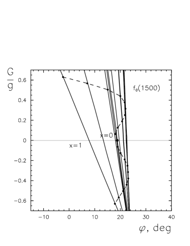
Figure 9:

Curves of correlations $(G/g,\varphi)$ for $f_{0}(1300)$, $f_{0}(1500)$, $f_{0}(1750)$ and $(g/G,\varphi)$ for $f_{0}(1420\;^{+\;150}_{-70})$. at ten fixed values of $x$; dotted curves stand for maximal accumulation of the gluonium component, $W_{gluonium}=40\%$.

Figure 10:

The evolution of $\varphi$ in the $q\bar{q}$ component $q\bar{q}=n\bar{n}\cos\varphi+s\bar{s}\sin\varphi$ at maximal accumulation of the gluonium component, $W_{gluonium}=40\%$; solid curves stand for positive $G/g$ and dotted ones to negative $G/g$. For $f_{0}(1420\;^{+\;150}_{-70})$, the $\varphi$ does not depend on the value of the adopted $q\bar{q}$ component.

References

- [1] V.V. Anisovich, A.A. Kondashov, Yu.D. Prokoshkin, S.A. Sadovsky, and A.V. Sarantsev, Yad. Fiz. 60, 1489 (2000) [Physics of Atomic Nuclei 60, 1410 (2000)].
- [2] V.V. Anisovich, V.A. Nikonov, and A.V. Sarantsev, ”Determination of hadronic partial widths for scalar-isoscalar resonances , , , and the broad state ”, hep-ph/0102338, Yad. Fiz., in press.
-
[3]
D. Alde et al., Zeit. Phys. C 66, 375 (1995);
Yu. D. Prokoshkin et al., Physics-Doklady 342, 473 (1995);
A. A. Kondashov et al., Preprint IHEP 95-137, Protvino, 1995;
F. Binon et al., Nuovo Cim. A 78, 313 (1983); 80, 363 (1984). -
[4]
V. V. Anisovich et al., Phys. Lett. B 323, 233 (1994);
C. Amsler et al., Phys. Lett. B 342, 433 (1995), 355, 425 (1995). -
[5]
S. J. Lindenbaum and R. S. Longacre, Phys. Lett. B 274, 492
(1992);
A. Etkin et al., Phys. Rev. D 25, 1786 (1982). - [6] D.E. Groom et al. (Particle Data Group), Eur. Phys. J. C15, 1 (2000).
-
[7]
G. Grayer et al., Nucl. Phys. B 75, 189 (1974);
W. Ochs, PhD Thesis, Münich University, (1974). - [8] V.V.Anisovich and A.V.Sarantsev, Phys. Lett. B 382 429 (1996).
- [9] V.V. Anisovich, Yu.D. Prokoshkin, and A.V. Sarantsev, Phys. Lett. B 389 388 (1996).
- [10] A.V. Anisovich and A.V. Sarantsev, Phys. Lett. B 413 137 (1997).
- [11] V.V. Anisovich, UFN 168, 481 (1998), [Physics-Uspekhi 41, 419 (1998)].
-
[12]
C. Amsler and F.E. Close, Phys. Rev. D 53, 295 (1996); Phys. Lett. B 353, 385 (1995);
V.V. Anisovich, Phys. Lett. B 364, 195 (1995); Physics-Uspekhi, 38, 1179 (1995). - [13] V.V. Anisovich and V. A. Nikonov, Eur. Phys. J. A 8, 401 (2000).
- [14] M.N. Kienzle-Focacci, ”Two-photon collisions at LEP”, in Proceedings of the VIIIth Blois Workshop, Protvino, Russia, 28 June-2 July 1999, eds. V.A. Petrov, A.V. Prokudin, World Scientific, 2000.
- [15] V.A. Schegelsky, ” physics at LEP”, Talk given in Open Session of HEP Division of PNPI: On the Eve of the XXI Century”, 25-29 December 2000.
- [16] A. V. Anisovich and V. V. Anisovich, Phys. Lett. B 467, 289 (1999).
-
[17]
CMD-2 Collaboration: R. R. Akhmetshin et al., Phys.
Lett. B 462, 371 (1999); 462, 380 (1999);
SND Collaboration: M. N. Achasov et al., Phys. Lett. B 485, 349 (2000). - [18] A.V. Anisovich, V.V. Anisovich, and V.A. Nikonov ”Quark structure of from the radiative decays , , , and ”, hep-ph/0011191 (2000).
- [19] E.M. Aitala et al. (E791 Collaboration), Experimental evidence for the light and broad scalar resonance in decay, hep-ex/0007028 (2000).
-
[20]
A.V. Anisovich, C.A. Baker, C.J. Batty et al., Phys.
Lett. B 468, 309 (1999);
Nucl. Phys. A 651:253 (1999);
D. Barberis, F.G. Binon, F.E. Close et al., Phys. Lett. B 467, 296 (1999). - [21] A.V. Anisovich, V.V.Anisovich, and A.V. Sarantsev, Phys. Rev. D 62:051502 (2000).
-
[22]
G. t’Hooft, Nucl. Phys. B 72, 161 (1974);
G. Veneziano, Nucl. Phys. B 117, 519 (1976). - [23] D. Aston et al. Nucl. Phys. B 296, 493 (1988).
-
[24]
G.S. Bali et al., Phys. Lett. B 309, 378
(1993);
J. Sexton, A. Vaccarino, and D. Weingarten, Phys. Rev. Lett. 75, 4563 (1995);
C.J. Morningstar and M. Peardon, Phys. Rev. D 56 , 4043 (1997). - [25] A.V.Anisovich, V.V.Anisovich, Yu.D.Prokoshkin, and A.V.Sarantsev, Zeit. Phys. A 357, 123 (1997).
- [26] A.V.Anisovich, V.V.Anisovich, and A.V.Sarantsev, Phys. Lett. B 395, 123 (1997); Zeit. Phys. A 359, 173 (1997).
- [27] I.S. Shapiro, Nucl. Phys. A 122, 645 (1968).
- [28] I.Yu. Kobzarev, N.N. Nikolaev, and L.B. Okun, Sov. J. Nucl. Phys. 10, 499 (1970).
- [29] L. Stodolsky, Phys. Rev. D 1, 2683 (1970).
- [30] V.V.Anisovich, D.V.Bugg, and A.V.Sarantsev, Phys. Rev. D58:111503 (1998).
- [31] V.V.Anisovich, D.V.Bugg, and A.V.Sarantsev, Sov. J. Nucl. Phys. 62, 1322 (1999) [Phys. Atom. Nuclei 62, 1247 (1999).
- [32] V.V.Anisovich, D.V.Bugg, and A.V.Sarantsev, Phys. Lett. B 437, 209 (1998).
- [33] K. Peters and E. Klempt, Phys. Lett. B @@@
-
[34]
G. Parisi and R. Petronzio,
Phys. Lett. B 94, 51 (1980);
J.M. Cornwell and J. Papavassiliou, Phys. Rev. D 40, 3474 (1989);
V.V. Anisovich, S.M. Gerasyuta, and A.V. Sarantsev, Int. J. Modern Phys. A 6, 625 (1991);
D.B. Leinweber et al., Phys. Rev. D58: 031501 (1998). - [35] V.V.Anisovich, A.A.Kondashov, Yu.D.Prokoshkin, S.A.Sadovsky, and A.V.Sarantsev, Phys. Lett. B 355, 363 (1995).