Global Analysis with SNO:
Toward the Solution of the Solar Neutrino Problem

P. I. Krastev¹ and A. Yu. Smirnov^2,3

(1) Philips Analytical, Natick, MA 01760, USA
(2) The Abdus Salam International Centre for Theoretical Physics, I-34100 Trieste, Italy
(3) Institute for Nuclear Research of Russian Academy of Sciences, Moscow 117312, Russia

We perform a global analysis of the latest solar neutrino data including the Solar Neutrino Observatory (SNO) result on the $CC-$event rate. This result further favors the LMA MSW solution of the solar neutrino problem. The best fit values of parameters we find are: $\Delta m^{2}=(4.8-5.0)\cdot 10^{-5}$ eV², $\tan^{2}\theta=0.35-0.38$, $f_{B}=1.08-1.12$, and $f_{hep}=1-4$, where $f_{B}$ and $f_{hep}$ are the boron and $hep-$ neutrino fluxes in units of the corresponding fluxes in the Standard Solar Model (SSM). With respect to this best fit point the LOW MSW solution is accepted at 90 % C.L.. The Vacuum oscillation solution (VAC) with $\Delta m^{2}=1.4\cdot 10^{-10}$ eV², gives good fit of the data provided that the boron neutrino flux is substantially smaller than the SSM flux ($f_{B}\sim 0.5$). The SMA solution is accepted at about $3\sigma$ level. We find that vacuum oscillations to sterile neutrino, VAC(sterile), with $f_{B}\sim 0.5$ also give rather good global fit of the data. All other sterile neutrino solutions are strongly disfavored. We check the quality of the fit by constructing the pull-off diagrams of observables for the global solutions. Maximal mixing is allowed at $3\sigma$ level in the LMA region and at 95 % C.L. in the LOW region. Predictions for the day-night asymmetry, spectrum distortion and ratio of the neutral to charged curent event rates, [NC]/[CC], at SNO are calculated. In the best fit points of the global solutions we find: $A_{DN}^{CC}\approx(7-8)\%$ for LMA, $\sim 3\%$ for LOW, and $(2-3)\%$ for SMA. In the LMA region the asymmetry can be as large as 15 - 20 %. Observation of $A_{DN}^{CC}>5\%$ will further favor the LMA solution. It will be difficult to see the distortion of the spectrum expected for LMA as well as LOW solutions. However, future SNO spectral data can significantly affect the VAC and SMA solutions. We present expected values of the BOREXINO event rate for global solutions.

Pacs numbers: 14.60.Lm 14.60.Pq 95.85.Ry 26.65.+t

1 Introduction

With the SNO result [1, 2] on the $CC-$rate, we now, for the first time ever, have more than $3\sigma$ evidence of flavor conversion of solar neutrinos. “Smoking guns” have indeed started to smoke. The statement, made first in the original publication by the SNO collaboration, is based on difference of the boron neutrino fluxes determined from the charged current ($CC-$) event rate in the SNO detector, and the $\nu e-$scattering event rate obtained by the SuperKamiokande (SK) [3] collaboration (and confirmed, albeit with smaller statistical significance, by SNO). Somewhat paradoxically, the absence of significant distortion of the boron neutrino spectrum at SuperKamiokande adds to the strength of this conclusion.

In general, the difference between the signals in the SNO and SK detectors can be due to:

1) appearance of the $\nu_{\mu},\nu_{\tau}-$ flux, or/and

2) distortion of the neutrino energy spectrum. If the suppression of the boron neutrino flux (due to some neutrino transformations) increases with neutrino energy, then the higher sensitivity to higher energies of the $CC-$reaction in SNO as compared with $\nu-e$ scattering in SK would explain the lower rate in SNO.

In fact, both reasons imply neutrino conversion. However, an absence of strong distortion of the boron neutrino spectrum, as found by SuperKamiokande and independently confirmed by SNO, leads to the conclusion that the main reason for the difference is the appearance of the $\nu_{\mu},\nu_{\tau}-$ flux.

From the SNO result and its comparison with the SK data one can immediately draw several conclusions:

• Strong deficit of the $\nu_{e}-$ flux with respect to the Standard Solar Model (SSM) predictions is found.

• There is a strong evidence that $\nu_{e}$ from the sun are converted to $\nu_{\mu},\nu_{\tau}$.

• There is no astrophysical solution of the solar neutrino problem. (For recent quantitative analysis see [4]).

• Solutions of the solar neutrino problem based on pure active - sterile conversion, $\nu_{e}\rightarrow\nu_{s}$, are strongly disfavored.

• More than half of the original $\nu_{e}-$flux is transformed to neutrinos of different type $\nu_{\mu}$, $\nu_{\tau}$, and possibly $\nu_{s}$, that is, the $\nu_{e}-$survival probability

  $$P<1/2.$$ (1)

  In fact, in assumption of pure active transition one gets $P=0.334\pm 0.22$ [2] which is just $\sim 1\sigma$ below 1/2. Clearly, if the sterile neutrino component is present in the flux, the survival probability is even smaller. The inequality (1), if confirmed, will have crucial implications for further experimental developments in the field, as well as for fundamental theory.

We know now with a high confidence that electron neutrinos produced in the center of the Sun undergo flavor conversion. However the specific mechanism of the conversion has not yet been identified. As we will see, only some extreme possibilities are excluded by adding the SNO result to the previously available solar neutrino data. A number of solutions still exist.

The SNO result changes the status of specific solutions to the solar neutrino problem. The changes can be immediately seen by comparing predictions for the $CC-$ event rate from global solutions found in the pre-SNO analysis [5, 6] with the SNO result. There are four solutions, three active and one sterile, which give predictions close to the SNO result:

$$R^{SNO}_{CC}\equiv\frac{SNO}{SSM}=0.347\pm 0.029.$$ (2)

1). The Large Mixing Angle MSW solution (LMA): the $3\sigma$ predictions interval, $R_{CC}=0.20-0.41$, covers the SNO result ($R_{CC}\equiv$ [CC] from [5]). The best fit point from the pre-SNO analysis, $R_{CC}=0.31$, is slightly ($\sim 1\sigma$) below the central value given by SNO. Therefore, SNO shifts the region of the LMA solution and the best fit point to larger values of mixing angles which correspond to larger survival probability.

2). The low $\Delta m^{2}$ (LOW) solution: the interval of predictions, $R_{CC}=0.36-0.42$, is above the SNO result. In the best fit point $R_{CC}$ is $2\sigma$ (experimental) higher the central SNO value. Therefore this solution is somewhat less favored, and SNO tends to shift the allowed region to smaller values of $\theta$ which correspond to smaller survival probability.

3). The vacuum oscillation solutions (VAC): the expected interval, $R_{CC}=0.33-0.42$, is also covering the SNO range, and the best fit value, $R_{CC}=0.38$, is just $1\sigma$ above the central SNO result. Therefore, SNO improves the status of this solution.

4). Vacuum oscillations to sterile neutrinos, VAC(sterile): the predicted interval, $R_{CC}=0.36-0.41$, with the best fit point 0.39, is only slightly higher than for the VAC(active) case. Here low rate predicted for SNO is due to difference of the thresholds in SNO and SK and to the steep increase of the suppression with neutrino energy. This solution survives the first SNO result.

Other solutions look less favorable in the light of the SNO result. In particular, the small mixing angle MSW (SMA) solution interval, $R_{CC}=0.37-0.50$, (especially its best fit point, 0.46, from the pre-SNO analysis) is substantially above the SNO rate. This solution is further disfavored by SNO. In fact, SMA predicts opposite energy dependence of the suppression on the neutrino energy to the one SNO prefers.

The Just-so²(active), SMA(sterile) and Just-so²(sterile) solutions predict practically the same rate for the SK and SNO and therefore are strongly disfavored.

The statements above are supported by detailed quantitative analysis of the solar neutrino data we have performed in this paper. The results of this analysis are described in the rest of this paper. Previously some of the same conclusions have been reported in [7, 8, 9, 10]; see also related studies [11, 12, 13, 14].

The paper is organized as follows: In Section 2 we present the results of the global analysis of the solar neutrino data. We construct the pull-off diagrams of available observables for the found global solutions. In Section 3 we consider specifics of global solutions and their implications. We evaluate the quality of the data fit in each of the global solutions. We calculate predictions for the day-night asymmetry and spectrum distortion in Section 4. Finally, prospects for identifying the solution to the solar neutrino problem are discussed in Section 5.

2 Global analysis and pull-off diagrams

We describe here the results of the global analysis of the solar neutrino data. We find global solutions (sets of oscillation parameters and solar neutrino fluxes which explain the solar neutrino data) and determine the goodness of fit (g.o.f.) in the best fit points. We perform diagnostics of the global solutions by checking their stability with respect to variations in the analysis and to uncertainties in the original solar neutrino fluxes. To check the quality of the fit we construct the pull-off diagrams for the observables.

2.1 Features of the analysis

We follow the procedure of the analysis developed in our previous publications [15, 16, 17, 5] in collaboration with John Bahcall. We also describe some additional features, which should be taken into account when comparing our results with those obtained by other groups.

In our global analysis we use: (i) the $Ar-$production rate from the Homestake experiment [18], (ii) the $Ge-$production rate from SAGE [19], (iii) the combined $Ge-$production rate from GALLEX and GNO [20, 21], (iv) the $CC-$event rate measured by SNO [1], (v) the Day and Night energy spectra measured by SuperKamiokande [3].

Following the procedure outlined in [5] we do not include the total rate of events in the SK detector, which is not independent from the spectral data. In our standard global analysis, we use 4 rates and 38 spectral data, a total of 42 data points. The number of free parameters and the number of d.o.f. are different in different analyses and we will specify them later.

The solar neutrino fluxes are taken according to SSM BP2000 [22] with the corrected (due to improved measurement of the solar luminosity) boron neutrino flux $F^{SSM}_{B}=5.05\cdot 10^{6}$ cm^-2 c^-1. We denote by $f_{B}$ and $f_{hep}$ the fluxes of the boron and $hep-$neutrinos measured in units of the BP2000 fluxes.

The analysis of the data is performed in terms of two neutrino mixing characterized by the mass squared difference $\Delta m^{2}$ and the mixing parameter $\tan^{2}\theta$. We consider conversion into pure active or pure sterile neutrinos.

We perform the $\chi^{2}$ test of various oscillation solutions by calculating

$$\chi^{2}_{global}=\chi^{2}_{rate}+\chi^{2}_{spectrum},$$ (3)

where $\chi^{2}_{rate}$ and $\chi^{2}_{spectrum}$ are the contributions from the total rates and from the SuperKamiokande day and night spectra correspondingly. Each of the entries in Eq.(3) is a function of the four parameters ($\Delta m^{2}$, $\tan^{2}\theta$, $f_{B}$ and $f_{hep}$). It is an important feature of our approach [5] that at each step of the minimization process these parameters are kept the same in each of the two entries on the right hand side of Eq. (3).

2.2 Free flux fit

We perform the fit to the experimental data treating the boron neutrino flux, $f_{B}$, and the $hep-$neutrino flux, $f_{hep}$, as free parameters. There are several reasons to consider $f_{B}$ and $f_{hep}$ as free parameters (for earlier work in this context see [23]):

1. These fluxes have the largest uncertainties in the SSM (see however, [24]).

2. The goal of the solar neutrino studies is to find directly from the solar neutrino data both the oscillation parameters and the neutrino fluxes. The free flux analysis is the way to achieve this goal.

3. Comparing the fluxes $f_{hep}$ and $f_{B}$ found from the free flux analysis with the SSM fluxes we can estimate the plausibility of the fit and the reliability of the solutions. Clearly, strong deviation of the fluxes for a given solution from the SSM values will indicate certain problems with either the solution or the SSM predictions.

4. Last, but not least, this fit is the most conservative one regarding the exclusion of certain scenarios.

Table 1: Best-fit values of the parameters $\Delta m^{2}$, $\tan^{2}\theta$, $f_{B}$ and $f_{hep}$ from the free flux analysis. The minimum $\chi^{2}$ and the corresponding g.o.f. are given in the last two columns. The number of degrees of freedom is 38: 4 rates (Homestake, SAGE, Gallex/GNO, SNO) + 38 SK spectra points - 4 parameters.

Solution	$\Delta m^{2}$/$\rm eV^{2}$	$\tan^{2}\theta$	$f_{B}$	$f_{hep}$	$\chi^{2}_{min}$	g.o.f.
LMA	$4.8\times 10^{-5}$	0.35	1.12	4	29.2	0.85
VAC	$1.4\times 10^{-10}$	0.40 (2.5)	0.53	6	32	0.74
LOW	$1.1\times 10^{-7}$	0.66	0.88	2	34.3	0.64
SMA	$6.0\times 10^{-6}$	$1.9\times 10^{-3}$	1.12	4	40.9	0.34
Just So2	$5.5\times 10^{-12}$	1.0	0.44	0	45.8	0.18
VAC(sterile)	$1.4\times 10^{-10}$	0.38 (2.6)	0.54	9	35.1	0.60
Just So2(sterile)	$5.5\times 10^{-12}$	1.0	0.44	0	46.2	0.17
SMA(sterile)	$3.8\times 10^{-6}$	$4.2\times 10^{-4}$	0.52	0.2	48.2	0.12
LMA(sterile)	$1.0\times 10^{-4}$	0.33	1.14	0	49.0	0.11
LOW(sterile)	$2.0\times 10^{-8}$	1.05	0.83	0	49.2	0.11

Thus, together with $\Delta m^{2}$ and $\tan^{2}\theta$, there are 4 free parameters and therefore 42 - 4 = 38 d.o.f. in the $\chi^{2}$-fit. In Table 1 we show the best fit values of the parameters $\Delta m^{2}$, $\tan^{2}\theta$, $f_{B}$, $f_{hep}$ for different solutions of the solar neutrino problem. We also give the corresponding values of $\chi^{2}_{min}$ and the goodness of the fit. Several remarks are in order.

The absolute $\chi^{2}$ minimum: $\chi^{2}=29.2$ is in the LMA region. Such a low $\chi^{2}$ for 38 d.o.f. is mainly due to the small spread of the experimental points in both the day and the night SK spectra. Similar situation is realized for the LOW solution. The SuperKamiokande day and night spectra can be especially well described by solutions which predict a bump in the survival probability at $E=6-8$ MeV and a dip at $E=10-11$ MeV. This is the case of VAC solutions (both active and sterile) with large $hep-$flux. It is for this reason VAC solutions have high goodness of the global fit. According to the Table 1 the VAC(sterile) solution is in the third position after LMA and VAC(active) and its fit is even better than the one of LOW solution. The VAC(sterile) solution has, however, a number of problems which we will discuss in the next section.

For LMA, LOW and SMA solutions values of $f_{B}$, agree with the SSM predictions within $1\sigma$ theoretical uncertainty ($\sim 18$ %). All VAC solutions and SMA(sterile), as well as Just-so² solutions, appear with a boron flux which is $3\sigma$ below the SSM boron neutrino flux. For the $hep-$neutrino flux the VAC and SMA solutions imply significant (factors 4 - 6) deviation from the central SSM value. The VAC(sterile) requires as large as 9 SSM $hep-$neutrino flux.

For VAC solutions the matter effect is negligible and in the Table 1, two “symmetric” values of $\tan^{2}\theta$: $\tan^{2}\theta_{1}=1/\tan^{2}\theta_{2}$ correspond to mixing in normal and dark (in brackets) sides of the parameter space.

Even within this conservative analysis the LMA(sterile) and LOW(sterile) solutions give a very bad fit and in what follows we will not discuss them.

Just-so²(active) and Just-so²(sterile) give very similar description of the data. So, we will present results for one of them.

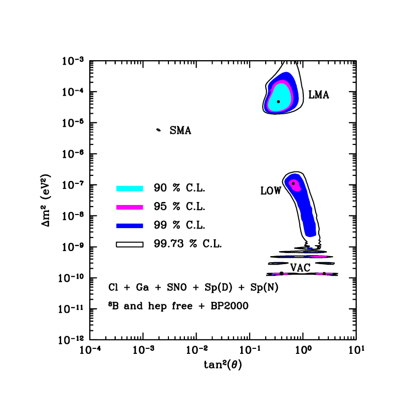
Figure 1: Global solutions from free flux analysis. The boron and $hep-$ neutrino fluxes are considered as free parameters. The best fit points are marked by dark circles. The absolute minimum of the $\chi^{2}$ is in the LMA region. The allowed regions are shown at 90%, 95%, 99% and 99.73% C.L. with respect to the global minimum in the LMA region.

In Fig. 1 we show contours of constant (90, 95, 99, 99.73 %) confidence level with respect of the absolute minimum in the LMA region. Following the same procedure as in [5] the contours have been constructed in the following way. For each point in the $\Delta m^{2}$, $\tan^{2}\theta$ plane we find minimal value $\chi^{2}_{min}(\Delta m^{2},\tan^{2}\theta)$ varying $f_{B}$ and $f_{hep}$. We define the contours of constant confidence level by the condition

$$\chi^{2}_{min}(\Delta m^{2},\tan^{2}\theta)=\chi^{2}_{min}(LMA)+\Delta\chi^{2}~{},$$ (4)

where $\chi^{2}_{min}(LMA)=29.3$ is the absolute minimum in the LMA region and $\Delta\chi^{2}$ is taken for two degrees of freedom.

To clarify the role of the $hep-$neutrino flux we present in Table 2 the result of the $\chi^{2}$ analysis when $f_{hep}=1$ and treat only $f_{B}$ as a free parameter. As follows from the Table 2, fixing the flux $f_{hep}$ leads to rather small change of the oscillation parameters. At the same time, the constraint $f_{hep}=1$ lowers a goodness of the fit of solutions which imply large value of $f_{hep}$ in the free flux analysis. We get $\Delta\chi^{2}=1.8$ for VAC(sterile), $\Delta\chi^{2}=1.4$ for SMA and $\Delta\chi^{2}=1.4$ for VAC(active). Notice that now VAC(sterile) is shifted to the fourth position.

According to Ref. LABEL:hepfl the calculated $hep-$ neutrino flux has about 20% uncertainty. Therefore solutions which require large $f_{hep}$ (2 - 9) are disfavored and the results of the fit with $f_{hep}=1$ look more relevant.

Table 2: Best-fit values of the parameters $\Delta m^{2}$, $\tan^{2}\theta$ and $f_{B}$ from the global analysis with $f_{hep}=1$. The minimum $\chi^{2}$ and the corresponding g.o.f. are given in the last two columns. The number of degrees of freedom is 39: 4 rates (Homestake, SAGE, Gallex/GNO, SNO) + 38 SK spectral points - 3 parameters.

Solution	$\Delta m^{2}$/$\rm eV^{2}$	$\tan^{2}\theta$	$f_{B}$	$\chi^{2}_{min}$	g.o.f.
LMA	$5.0\times 10^{-5}$	0.36	1.1	30.1	0.85
VAC	$1.4\times 10^{-10}$	0.363 (2.7)	0.54	33.4	0.72
LOW	$1.1\times 10^{-7}$	0.69	0.86	34.5	0.67
SMA	$5.5\times 10^{-6}$	$1.9\times 10^{-3}$	1.04	42.2	0.33
Just So2	$5.5\times 10^{-12}$	1.0	0.44	46.4	0.19
VAC(sterile)	$1.4\times 10^{-10}$	0.35 (2.9)	0.55	36.9	0.57
SMA(sterile)	$3.8\times 10^{-6}$	$4.2\times 10^{-4}$	0.52	48.6	0.14

2.3 SSM restricted global fit

In order to check the significance of the SSM restriction on the boron neutrino flux we have performed the fit to the data adding to the $\chi^{2}$ sum in Eq. (3) the term

$$\left(\frac{f_{B}-1}{\sigma_{B}}\right)^{2}~{},$$ (5)

where $\sigma_{B}=0.18$ is the average (of the upper and lower) $1\sigma$ theoretical error of the flux in BP2000 model [22]. With the term (5) included in our global $\chi^{2}$ we, in a way, treat the SSM prediction for the boron neutrino flux as independent “measurement” and consider it as an additional degree of freedom. This procedure makes sense because a significant contribution to the error in SSM determination of the boron neutrino flux comes from the measurements of the $p-Be$ cross-section.

One “technical” remark is in order. Our approach differs from analyses where the boron neutrino flux is taken as a theoretical prediction from the SSM [8, 9]. In the latter case the term (5) is absent, the central SSM value is used in the predictions of observables and the theoretical errors on the boron neutrino flux are added to the experimental errors.

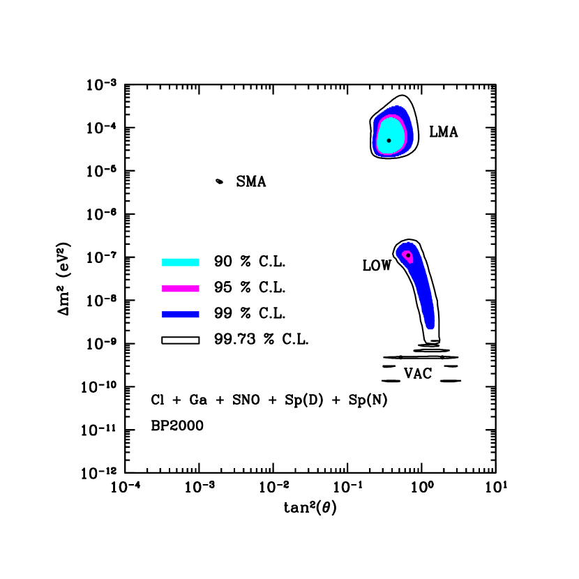
Figure 2: Global solutions for the SSM restricted boron neutrino flux. $hep-$ neutrino flux is free. The best fit points are marked by dark circles. The absolute minimum of the $\chi^{2}$ is in the LMA region. The allowed regions are shown at 90%, 95 %, 99% and 99.73% with respect to the global minimum in the LMA region.

In Table 3 and Fig. 2 we present the results of the fit with SSM constrained boron neutrino flux. As expected, the most significant changes in comparison with the free flux analysis (Table 1) appear in those solutions and regions of the oscillation parameters which imply strong deviation of $f_{B}$ from 1. Our results show that mostly the best fit points, as well as the $\chi^{2}_{min}$ and goodness of the VAC(active), Just-so², VAC(sterile) and SMA(sterile) solutions are affected. Thus, for the VAC(active) solution $\Delta\chi^{2}_{min}=3.4$, for VAC(sterile): $\Delta\chi^{2}_{min}=6.2$. Moreover, the best fit VAC solution shifts to another point of oscillation parameters in agreement with results of other groups. There is no significant change of the LMA, LOW and SMA best fit points and goodness of the fit.

Table 3: Best-fit values of the parameters $\Delta m^{2}$, $\tan^{2}\theta$, $f_{B}$ and $f_{hep}$ from the SSM restricted global analysis. $f_{hep}$ is considered as a free parameter. The minimum $\chi^{2}$ and the corresponding g.o.f. are given in the last two columns. The number of degrees of freedom is 40: 4 rates (Homestake, SAGE, Gallex/GNO, SNO) + 38 SK spectral points + 1 ($f_{B}$) - 3 parameters.

Solution	$\Delta m^{2}$/$\rm eV^{2}$	$\tan^{2}\theta$	$f_{B}$	$f_{hep}$	$\chi^{2}_{min}$	g.o.f.
LMA	$5.0\times 10^{-5}$	0.36	1.10	4.0	29.5	0.84
SMA	$5.5\times 10^{-6}$	$1.9\times 10^{-3}$	1.10	4.0	41.2	0.33
LOW	$1.1\times 10^{-7}$	0.66	0.88	2.0	34.7	0.62
VAC	$4.8\times 10^{-10}$	1.9	0.72	0.0	35.4	0.59
Just So2	$5.5\times 10^{-12}$	1.4	0.44	1.0	55.4	0.03
VAC(sterile)	$1.4\times 10^{-10}$	2.63	0.55	8.0	41.3	0.33
SMA(sterile)	$4.0\times 10^{-6}$	$4.8\times 10^{-4}$	0.54	2.0	54.5	0.04

In Fig. 2 we show the contours of constant (90, 95, 99, 99.73 %) confidence level for two degrees of freedom with respect to the absolute minimum in the LMA region.

2.4 Analysis of “Rates Only”

To clarify the relative significance of the total rates and the SK spectrum in the global analysis of the data we have performed a fit to the rates in the 4 experiments: Homestake, SAGE, GALLEX/GNO, SNO and SK. In this analysis we use the total rate of events in SK but do not use the SK energy spectrum of the recoil electrons. The results of the $\chi^{2}$ test are summarized in the Table 4.

Notice that with the SNO result the SMA solution does not give anymore the best fit to the “rates only”, in contrast with pre-SNO analyses. The best fit is obtained in the VAC solution region. However, parameters of this solution differ significantly from the parameters of the global solution when spectral data are included.

The “rates only” fit shifts the LMA region to smaller $\Delta m^{2}$. The LOW solution is practically unchanged. Now VAC(sterile) and LOW have low goodness of fit.

Notice that in the absence of the spectral data the value of $\chi^{2}_{min}$ is comparable or larger than the number of d.o.f. .

Table 4: Best-fit values of the parameters $\Delta m^{2}$ and $\tan^{2}\theta$ from the “Rates Only” analysis. The minimum $\chi^{2}$ and the corresponding g.o.f. are given in the last two columns. The number of degrees of freedom is 3: 5 rates (Homestake, SAGE, Gallex/GNO, SNO, SK) - 2 parameters.

Solution	$\Delta m^{2}$/$\rm eV^{2}$	$\tan^{2}\theta$	$\chi^{2}_{min}$	g.o.f.
LMA	$2.9\times 10^{-5}$	0.36	3.55	0.31
SMA	$7.9\times 10^{-6}$	$1.4\times 10^{-3}$	5.1	0.16
LOW	$1.0\times 10^{-7}$	0.66	7.9	0.05
VAC	$7.9\times 10^{-11}$	3.5	2.24	0.52
Just-so2	$5.5\times 10^{-12}$	2.0	16.4	0.0009
SMA(sterile)	$4.4\times 10^{-6}$	$1.0\times 10^{-3}$	17.4	0.0006
VAC(sterile)	$1.0\times 10^{-10}$	$0.35$	6.4	0.094

2.5 Pull-off diagrams

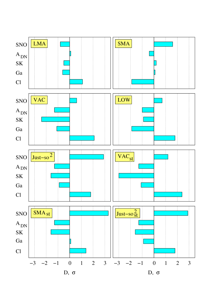
Figure 3: Pull-off diagrams for global solutions. Shown are deviations of predictions for the $Ar-$production rate $Ge-$production rate, SK rate, the day-night asymmetry at SK, and the SNO rate from experimentally measured values. The pull-offs are expressed in the units of 1 standard deviation, $1\sigma$.

In order to check the quality of the fits we have calculated predictions for the available observables in the best fit points of the global solutions found in the free flux analysis (see Table 5). Using these predictions we have constructed the “pull-off” diagrams (fig. 3) which show deviations, $D_{K}$, of the predicted values of observables $K$ from the central experimental values expressed in the $1\sigma$ unit:

$$D_{K}\equiv\frac{K_{bf}-K_{exp}}{\sigma_{K}},~{}~{}~{}~{}K\equiv Q_{Ar},~{}Q_{Ge},~{}R_{CC},~{}R_{\nu e},~{}A_{DN}^{SK}.$$ (6)

Here $\sigma_{K}$ is the one sigma standard deviation for a given observable $K$. We take the experimental errors only: $\sigma_{K}=\sigma_{K}^{exp}$. The theoretical errors are related mainly to the uncertainty in the boron neutrino flux. Since $f_{B}$ is treated as a free parameter we do not take into account its theoretical errors. The remaining theoretical errors are small and strongly correlated in $Q_{Ar}$, $R_{CC}$ and $R_{\nu e}$.

Table 5: Values of the total rates in $Cl-$ , $Ga-$, SK and SNO experiments in the best fit points of global solutions found in the free flux analysis. The rates in the radiochemical experiments are given in SNU. For SuperKamiokande and SNO the ratios of the best fit rates to the rates predicted in the SSM is given.

Solution	$Cl$	$Ga$	$SK$	$SNO$
LMA	2.89	71.3	0.452	0.323
SMA	2.26	74.4	0.463	0.396
LOW	3.12	68.5	0.446	0.368
VAC	3.13	70.2	0.423	0.364
Just So2	3.00	70.8	0.434	0.434
SMA(sterile)	2.93	75.5	0.435	0.445
VAC(sterile)	3.24	69.9	0.414	0.381
Just So2	3.01	70.9	0.434	0.435

The diagrams are good diagnostics of the fit. They allow one to pin down problems that some of the solutions have and to elaborate criteria for further checks.

According to Fig. 3 only the LMA solution does not have strong deviations of predictions from the experimental results. LOW, VAC and SMA solutions give somewhat worser fit to the data. The fit from other solutions is very bad.

The pull-off diagrams give some clarification to a common worry, namely that the high statistics SK experiment (in particular its spectral data) overwhelms the rates data in the global analysis. In particular, solutions, which are strongly disfavored by the rates, give a good fit when spectral data are included.

This problem can be approached in a different way: one can use just one parameter, e.g., the first moment, which describes possible distortions of the recoil electron energy spectrum [25].

3 Global solutions: properties and implications

Here we evaluate the status of global solutions using the following criteria:

1. Goodness of the global fit in the free flux analysis.

2. Deviation of the boron and $hep-$neutrino fluxes found in the free flux analysis from the SSM values fluxes, that is, the deviation of $f_{B}$ and $f_{hep}$ from 1.

3. Goodness of the fit in the SSM restricted analysis and in the “Rates only” analysis.

4. Stability of the solution with respect to variations of the analysis.

5. Quality of the fit of the individual observables; features of the pull-off diagram. A deviation by more than $3\sigma$ for some observables is a clear signal for trouble.

We identify solutions which pass all of these criteria.

3.1 The best fit solution: LMA

SNO further favors the LMA solution [26]. In all global analyses, in which the SK spectral data is included, LMA gives minimal $\chi^{2}$. The best fit point from the free flux analysis is:

$$\Delta m^{2}=4.8\cdot 10^{-5}~{}{\rm eV}^{2},~{}~{}~{}\tan^{2}\theta=0.35,~{}~{}~{}f_{B}=1.2,~{}~{}~{}f_{hep}=4.0~{}.$$ (7)

Large $f_{hep}$ is needed to account for some excess of the SK events in the high energy part of the spectrum. For $f_{hep}=1$, values of the oscillation parameters are practically the same as in the free flux analysis (see Table 2), and the goodness of the fit is even slightly higher. The boron neutrino flux is 10% higher than central value in the SSM: $F_{B}=f_{B}\cdot F_{B}^{SSM}=5.66\cdot 10^{6}$ cm^-2 c^-1 being however within $1\sigma$ deviation. This flux is rather close to the central value extracted from the SNO and SK data [1].

The fit of the data with the SSM restricted $f_{B}$ gives minimum of $\chi^{2}$ at practically the same values of parameters as in (7).

The values of the oscillation parameters (7) found here are very close to the values found by other groups [8, 9]. This shows that the solution is robust and doesn’t change with the type of analysis.

Notice that the SNO data lead to a shift of the best fit point (as well as the whole region) to larger values of $\tan^{2}\theta$ as was discussed in the introduction.

According to the pull-off diagram, the LMA solution reproduces observables at $\sim 1\sigma$ or better. The largest deviation is for the $Ar-$production rate: the solution predicts $1.1\sigma$ larger rate than the Homestake result.

The “Rates only” analysis shifts the best fit point to smaller $\Delta m^{2}$.

Considering the allowed regions at different confidence levels we find the following:

1). $\Delta m^{2}$ is rather sharply restricted from below by the day-night asymmetry of the SK event rate: $\Delta m^{2}>2\cdot 10^{-5}$ eV² at 99.73% C.L. .

2). The upper bound on $\Delta m^{2}$ is of great importance for future experiments, in particular for the neutrino factories [27]. We find from the free flux fit (CHOOZ bound is not included)

$$\Delta m^{2}\leq\left\{\begin{array}[]{ll}1.9\times 10^{-4}~{}{\rm eV}^{2},&~{}~{}90\%~{}{\rm C.L.}\\ 2.3\times 10^{-4}~{}{\rm eV}^{2},&~{}~{}95\%~{}{\rm C.L.}\\ 4.3\times 10^{-4}~{}{\rm eV}^{2},&~{}~{}99\%~{}{\rm C.L.}\\ \end{array}\right..$$ (8)

Similar results can be obtained from the analysis in Ref. [8] where also CHOOZ data [28] have been taken into account. The CHOOZ bound becomes important for larger than $\Delta m^{2}\sim 8\times 10^{-4}{\rm eV}^{2}$ where it modifies the $3\sigma$ contour.

The fit with SSM restricted $f_{B}$ gives stronger bound on $\Delta m^{2}$. Instead of the limits in Eq. (8) we get the upper bounds $1.7\cdot 10^{-4}$, $2.1\cdot 10^{-4}$, and $3.1\cdot 10^{-4}$ eV² for 90, 95 and 99 % C.L. correspondingly.

3). The SNO and SK results (evidence of $\nu_{\mu}$, $\nu_{\tau}$ appearance) give an important lower limit on mixing:

$$\tan^{2}\theta>0.2~{}~{}~{}~{}99\%~{}{\rm C.L.}.$$ (9)

4). Maximal mixing is allowed only at the $\sim 3\sigma$ level:

$$\tan^{2}\theta\geq 1~{}~{}~{}~{}{\rm for}~{}~{}\Delta m^{2}=(4-10)\cdot 10^{-5}~{}~{}{\rm eV}^{2},~{}~{}~{}~{}~{}~{}~{}99.73\%~{}~{}{\rm C.L.}.$$ (10)

In spite of the shift of the best fit point to larger values of $\Delta{m}^{2}$ the C.L. for acceptance of maximal mixing is not lower than it was before the SNO result. The reason is that the SNO rate corresponds to a survival probability smaller than 1/2, which disfavors maximal mixing.

Similar result follows from the analysis in Ref.[8] where it was found that maximal mixing (at $3\sigma$ level) is allowed for $\Delta{m}^{2}=(4-20)\cdot 10^{-5}$ eV².

In the fit with the SSM restricted $f_{B}$, maximal mixing is even more disfavored: $\tan^{2}\theta<0.9$ at 99.73 % C.L..

3.2 Large or Small? The fate of SMA

The fate of the SMA solution, the only solution which is based on small mixing, is of great importance for future developments in both theory and experiment.

We find that the SMA solution does not appear at $3\sigma$ level (with respect to the global minimum) in the free flux fit. The best fit point parameters are:

$$\Delta m^{2}=6.0\cdot 10^{-6}~{}{\rm eV}^{2},~{}~{}~{}\tan^{2}\theta=0.0019,~{}~{}~{}f_{B}=1.12,~{}~{}~{}f_{hep}=4.$$ (11)

SNO shifts the local minimum to substantially larger mixing angles in comparison with the pre-SNO result. This is a consequence of appearance of the $\nu_{\mu}/\nu_{\tau}-$ flux, which implies large transition probability and therefore large mixing angles. At such a large $\tan^{2}\theta$ one expects significant distortion of the boron neutrino spectrum (see sect. 4).

Important feature of the solution is large flux of the $hep-$neutrinos. It is this large flux which, together with correlated systematic error and $f_{B}>1$, makes possible to get a reasonable description of the SK energy spectrum. If the SSM value is taken for the $hep-$neutrino flux (see Table 2) the $\chi^{2}$ increases by $\Delta\chi^{2}=1.4$.

These results are in agreement with those obtained in [8]. In [9], the SMA is accepted at lower than 99% level. Surprizingly, in this analysis the SNO result shifts mixing to even smaller values: the best fit value from [9] is at $\tan^{2}\theta=4\cdot 10^{-4}$.

Before the SNO result, the SMA solution was always giving the best fit to the total rates. Inclusion of the $CC-$event rate measured by SNO moves the SMA solution to third position, after VAC and LMA. Furthermore, the fit is no longer good: $\chi^{2}_{min}=5.1$ for 3 d.o.f.. From the pull-off diagram we find that there is a tension between the SNO and Homestake rates: The SNO data ($CC-$rate) requires rather small survival probability for boron electron neutrinos. Furthermore Gallium experiments imply strong suppression of the Beryllium neutrino flux. This leads to low ($1.9\sigma$) $Ar-$ production rate. At the same time, according to fig. 3 the $CC-$event rate is $1.7\sigma$ higher than the SNO result.

For mixing angle corresponding to the best fit point (11) one expects significant regeneration effect in the core-night bin [29] due to parametric enhancement of oscillations for the core crossing trajectories [30]. However, the day and the night spectra we used in our analysis are not sensitive to this feature. The zenith angle distribution of events measured by SK does not show any core enhancement [3]. Inclusion of this information in the global analysis will further disfavor the SMA solution.

3.3 LOW: next best?

For the best fit point of the free flux analysis we get:

$$\Delta m^{2}=1.1\cdot 10^{-7}~{}{\rm eV}^{2},~{}~{}~{}\tan^{2}\theta=0.66,~{}~{}~{}f_{B}=0.88,~{}~{}~{}f_{hep}=2.0.$$ (12)

If the $hep-$neutrino flux is fixed at its SSM value, $f_{hep}=1$, the best fit point shifts to larger mixing: $\tan^{2}\theta=0.69$. Notice that the solution implies $\sim 1\sigma$ lower boron neutrino flux than in SSM.

In the analysis with SSM restricted $f_{B}$ the best fit point is the same as in (12)

The LOW solution gives rather poor fit of the total rates $\chi^{2}=7.9$ for 3 d.o.f. (see Table 4). In the best fit point we get $2\sigma$ larger $Ar-$production rate and $1.9\sigma$ lower $Ge-$production rate. It is this case when the overwhelming spectral information “hides” some problems with total rates in the global fit. The use of a single parameter for description of the spectrum distortion gives much lower goodness of the fit for the LOW solution as compared with the LMA solution [25].

3.4 VAC - oscillation solution is back ?

As anticipated from the comparison of the pre-SNO predictions with the SNO result the VAC solution improves its status. Indeed, in the best fit point of the free flux analysis:

$$\Delta m^{2}=1.4\cdot 10^{-10}{\rm eV}^{2},~{}~{}~{}\tan^{2}\theta=0.40~{}(2.5),~{}~{}~{}f_{B}=0.53,~{}~{}~{}f_{hep}=6.0.$$ (13)

$\chi^{2}$ is even lower than the LOW solution has. The solution with parameters (13) has been found in the pre-SNO analysis [5], but before the SNO result the goodness of the fit was substantially lower in comparison with other solutions.

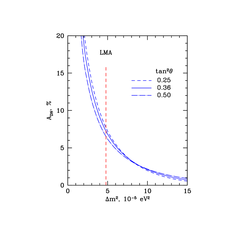
Figure 4: The dependence of the Day-Night asymmetry of the $CC-$event rate measured at SNO on the $\Delta m^{2}$ for different values of the mixing angle. The oscillation parameters are taken from the LMA allowed region. The best fit value of $\Delta m^{2}$ is marked by the vertical dotted line.

The solution gives very good description of the SK energy spectrum. The $\chi^{2}$ is substantially smaller than the number of degrees of freedom. The solution reproduces rather precisely the bump in both the night and the day spectra at (7 - 8) MeV and the dip at (11 - 12) MeV. (This features can be well seen in fig. 4e from the Ref. [31].) The bump in the spectrum originates from the first maximum of the oscillation probability which corresponds to the oscillation phase $2\pi$. Above the bump the probability decreases with energy and the increase of $R_{\nu e}$ at $E>12$ MeV is due to large flux of the $hep-$neutrinos.

Notice that an excellent description of the spectrum requires non-maximal mixing, otherwise the distortion is very strong. Value of $\sin^{2}2\theta$ which immediately determines the depth of oscillations should be about $0.8$. Then to compensate for rather large survival probability and to explain the SNO result one needs to assume a small ($f_{B}\sim 0.5$) original boron neutrino flux.

However, there are several problems with this solution. It requires substantially ($\sim 3\sigma$) lower original boron neutrino flux than in SSM and substantially higher original $hep-$neutrino flux: $f_{hep}=6$. In the fit with $f_{hep}=1$ the $\chi^{2}$ increases by $\Delta\chi^{2}=1.4$.

For this solution one predicts the seasonal asymmetry due to oscillations $A\approx-0.6A_{0}$, where $A_{0}\sim 7\%$ is the asymmetry due to the geometrical factor only ($1/R^{2}$ change of the flux). Thus one expects a suppressed seasonal asymmetry in contrast with observations.

The solution gives rather good fit to the rates. Although in the “Rates only” analysis the best fit point shifts to a different island in parameter space. According to the pull-off diagram, the solution predicts $2.1\sigma$ higher $Ar-$production rate and $2.6\sigma$ lower SK rate, and no day-night asymmetry.

The SSM restricted global fit shifts the best fit point to an “island” centered around

$$\Delta m^{2}=4.8\cdot 10^{-10}~{}{\rm eV}^{2},~{}~{}~{}~{}\tan^{2}\theta=1.9.$$ (14)

Now $f_{B}=0.72$. This solution was found by other groups too. The solution in the same “island” of the oscillation parameter space already appeared before (after 508 days of SK operation) when a significant excess of events at the high energy part of the spectrum was observed. The solution was later excluded by SK data on the spectrum. After the SNO result it re-appeared again. The solution can reproduce some bump at $E\sim 8$ MeV and increase of $R_{\nu e}$ at the high energies.

Thus, in the VAC region there are three local minima (two of them are degenerate) with rather close $\chi^{2}$. Small variations in the analysis shift the best fit VAC point from one minimum to another.

Although the VAC solution provides a very good fit to the data in the free flux global analysis, it does not pass additional criteria of quality. It requires very strong deviations of the boron and hep neutrino fluxes from the SSM values. The goodness of the fit becomes substantially worse when the SSM restrictions are imposed on these fluxes. There are significant deviations in the pull-off diagram.

The Just-so² solution looks extremely unlikely in the light of the SNO result. It gives a very poor fit to the rates. In fact, the fit is so bad that even the flat spectrum that it predicts, in agreement with the SK measurement, is not sufficient to make it plausible. Given the excellent fit of the LMA solution, the Just-so² solution is ruled out at 3$\sigma$ C.L.. This result is in agreement with Ref.[8]. Note that if SNO fails to observe a large day-night asymmetry, the situation might change and the Just-so² solution might reappear at about $\sim 3\sigma$ C.L..

3.5 How large is large mixing?

This question is crucial for theory. In a number of approaches to the bi-large mixing one gets mixing of the electron neutrino which is very close to maximal mixing (see [32] for a general discussion).

In the LMA region we find from the free flux analysis:

$$\tan^{2}\theta<\left\{\begin{array}[]{ll}0.68{}{}&95\%~{}~{}{\rm C.L.}\\ 0.82{}{}&99\%~{}~{}{\rm C.L.}\\ 1.05{}{}&99.73\%~{}~{}{\rm C.L.}\\ \end{array}\right.$$ (15)

and, as we discussed in sect. 3.1, maximal mixing is allowed at $\sim 3\sigma$ level for $\Delta m^{2}=(4-10)\cdot 10^{-5}$ eV². In the SSM restricted analysis the bounds become stronger.

In the LOW region we find $\tan^{2}\theta<0.9$ at 95% C.L.. Maximal mixing is accepted at slightly lower than 99% C.L. . in the range $(6\cdot 10^{-9}-3\cdot 10^{-7})$ eV² which covers LOW and the so called QVO (Quasi-Vacuum Oscillation) regions.

Maximal mixing is the best fit value of the Just-so² solution. Although this solution is ruled out at $3\sigma$ level in the global analysis. Notice, the fit of the data in the VAC region implies significant deviation from maximal mixing.

3.6 Do pure sterile solutions exist?

The best (and the only accepted at $3\sigma$ level) pure sterile solutions is the VAC(sterile), as could be expected from our pre-SNO analysis [5]. In the free flux analysis the solution appears at 90% C.L. already with the best fit point:

$$\Delta m^{2}=1.4\cdot 10^{-10}~{}{\rm eV}^{2},~{}~{}~{}\tan^{2}\theta=0.38~{}(2.6),~{}~{}~{}f_{B}=0.54,~{}~{}~{}f_{hep}=9.$$ (16)

Partially, the difference between the SK and SNO rates is explained by distortion of the spectrum: the suppression increases with energy and therefore the higher threshold at SNO leads to lower averaged survival probability. However, mainly the fit “shares” the deviations between SNO and SK: the solution requires $1.2\sigma$ higher SNO rate and significantly lower boron neutrino flux which gives a $\nu e-$ scattering rate $3.0\sigma$ below the SK result (see fig. 3). The free flux analysis without SK total rate does not locate this problem immediately. In principle, it should reappear in the fit of the spectrum with similar $\Delta\chi^{2}$ since the solution fits the shape of the spectrum rather well.

Notice that the parameters of this solution are very close to the parameters of VAC(active) apart from the two times larger $hep-$flux. So this solution leads to the same type of the spectrum distortion as the one described in sect. 3.4 with the bump at $E=7-8$ MeV and the dip at $E=11-12$ MeV.

In addition to a strong deviation of the $\nu e$ scattering event rate from the SK result, the solution predicts $2.1\sigma$ larger $Ar-$production rate. The fit worsens when SSM restrictions are imposed. For the SSM value of the $hep-$neutrino flux the best fit point shifts to a smaller mixing angle and the $\chi^{2}$ increases by $\Delta\chi^{2}=1.8$. In the analysis with SSM restricted $f_{B}$, the goodness of the fit drops further: $\Delta\chi^{2}=6.2$. In the fit of the rates the solution shifts to smaller $\Delta m^{2}$ where a description of the SK spectra becomes bad. Thus, the solution does not pass additional quality tests.

The SMA(sterile) solution gives a very bad fit since it leads (in contrast with the VAC solution) to a distortion of the boron neutrino spectrum with suppression which weakens with increase of energy. This solution contradicts the SNO result: $3.3\sigma$ higher rate is predicted.

Concerning sterile solutions one remark is in order. Better fit of the data can be obtained if more than 1 sterile neutrino participate in the conversion. Such a possibility is realized when solar neutrinos convert to the so called “bulk” neutrinos which propagate both in usual and in (large) extra space dimensions  [33]. From the four dimensions point of view the solar $\nu_{e}$ is transformed to several Kaluza-Klein mode of the bulk neutrino which show up as sterile neutrinos. In this case one can reproduce (with low $\chi^{2}$) the SK spectral data, and at the same time have better descriptions of the total rates (see [34] for recent analysis).

4 SNO: Predictions for the next step

Forthcoming results from SNO will include measurements of the day-night asymmetry and a more precise determination of the electron energy spectrum (higher statistics and lower energy threshold). Later results on the NC/CC ratio will be available. Predictions for these observables have extensively been discussed before [35, 36, 37, 38, 39, 40]. Here we sharpen the predictions using the latest solar neutrino data. We also calculate the expected values of the total event rate in the BOREXINO experiment which start to operate soon.

4.1 Day-Night asymmetry

We calculate the D-N asymmetry at SNO, $A_{DN}^{SNO}$, defined as

$$A_{DN}^{SNO}\equiv 2\frac{N-D}{N+D}$$ (17)

for the events above the threshold $E^{th}=6.75$ MeV.

We compare the asymmetry of the $CC-$ events at SNO with the asymmetry of the $\nu e-$events measured at SK: $A_{DN}^{SK}$. There are tree factors which can lead to substantially different SNO and SK asymmetries:

A “dumping” factor, $\eta_{dump}$, describes the suppression of the D-N asymmetry in the $\nu e-$ event rate due to the contribution of the $\nu_{\mu},\nu_{\tau}$ scattering to the signal. We get [16]

$$A_{DN}^{SNO}\propto\eta_{dump}A_{DN}^{SK},$$ (18)

where

$$\eta_{dump}=1+\frac{r}{(1-r)\bar{P}}~{}.$$ (19)

Here $r\equiv\sigma(\nu_{\mu})/\sigma(\nu_{e})$ is the ratio of cross-sections of the $\nu_{\mu}e-$ and $\nu_{e}e-$ scattering, and $\bar{P}$ is the averaged survival probability. Notice that with decrease of $\bar{P}$ the damping factor increases.

A second factor, $\eta_{thr}$, describes the effect of difference of the energy thresholds: 5 MeV for SK and 6.75 MeV for SNO. It also accounts for the larger minimum difference (the binding energy of the deutron, 1.44 MeV) between neutrino energy and electron energy in SNO.

A third factor, $\eta_{reg}$, is related to the difference of the geographical latitudes. Since the Sudbury mine is at higher latitude, the regeneration effect there is slightly weaker than at Kamioka.

The total difference between the SNO and SK asymmetries is the product of these three factors.

Let us consider now the predictions for the asymmetries for individual solutions.

1). LMA- solution. In Fig. 4 we show dependence of the asymmetry on $\Delta m^{2}$ for different values of $\tan^{2}\theta$ from the allowed region. The asymmetry decreases with increase of $\Delta m^{2}$ as $\sim 1/\Delta m^{2}$ for $\Delta m^{2}>4\cdot 10^{-5}$ eV² and at larger $\Delta m^{2}$ the decrease is faster due to effect of the adiabatic edge (see [17] for details). The dependence of asymmetry on $\tan^{2}\theta$ is rather weak. In the best fit point we get

$$A_{DN}^{SNO}=7.2\%~{}~{}~{}~{}(E^{th}=6.75~{}{\rm MeV}).$$ (20)

In the allowed region the asymmetry can take any value from practically zero to 15% at 90 % C.L.. At $3\sigma$ level it can reach 20 %. The asymmetry is maximal at the smallest possible values of $\Delta m^{2}$ and $\tan^{2}\theta$ within the allowed region. It increases with the energy threshold due to an increase of the regeneration factor: $f_{reg}\propto E/\Delta m^{2}$.

The expected asymmetry at SNO is substantially larger than at SK. In the best fit point we get $A_{DN}^{SK}=3.6\%$, thus $A_{DN}^{SNO}\approx 2\cdot A_{DN}^{SK}$. This difference can be easily understood considering the factors mentioned above. Indeed, for the best fit point the survival probability can be estimated as $\bar{P}\approx R_{SNO}/f_{B}$. Inserting numbers from the Table 5 we get from Eq. (19) $\eta_{dump}=1.6$. In the LMA region the asymmetry increases with $E_{th}$. The threshold factor equals $\eta_{thr}\sim 1.2$, and $\eta_{reg}$ is close to 1. As a result, the overall enhancement factor at SNO is about 2.

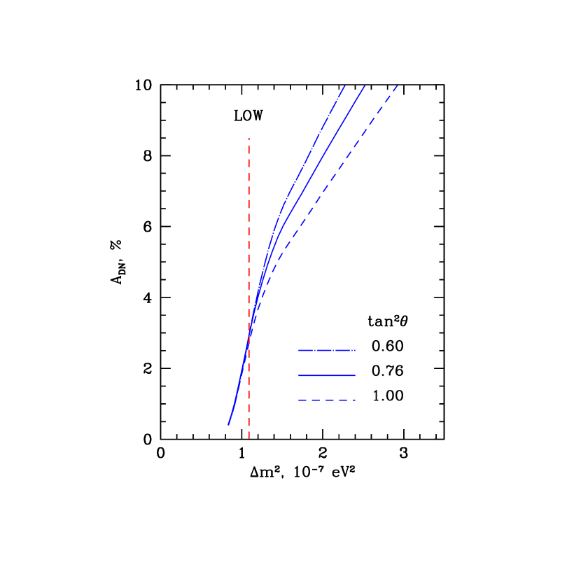
Figure 5: The same as in the Fig. 3a for the LOW solution. The dotted vertical lines mark the best fit values of $\Delta m^{2}$ from the free flux fit (left) and SSM restricted fit (right).

2). LOW solution. The dependence of the asymmetry on $\Delta m^{2}$ for different values of $\tan^{2}\theta$ from the allowed region is shown in Fig. 5. In the best fit point (of the free flux analysis)

$$A_{DN}^{SNO}=2.4\%~{}~{}~{}~{}(E^{th}=6.75~{}{\rm MeV}).$$ (21)

The asymmetry increases linearly with $\Delta m^{2}$ for $\Delta m^{2}>10^{-7}$ eV². It can reach 10 - 12 % at the upper border of the allowed ($3\sigma$) region. For $\Delta m^{2}<10^{-7}$ eV² the asymmetry decreases faster with $\Delta m^{2}$ due to effect of the non-adiabatic edge (see [17] for details). It depends weakly on the mixing angle.

Let us emphasize that the D-N asymmetry in the best fit point of the LOW solution is substantially smaller than the one in the LMA region. Thus, an observation of asymmetry $A_{DN}^{SNO}>5\%$ will strongly favor the LMA solution.

In the LOW region the D-N asymmetry at SNO is also larger than in the SK detector. However the difference here is not as large as in the LMA case. In the best fit point we get $A_{DN}^{SK}=2\%$, which results in $A_{DN}^{SNO}=1.2A_{DN}^{SK}$. There are two reasons for such a difference:

(i) The average survival probability is larger now (mixing angle is larger): $\bar{P}\approx R_{SNO}/f_{B}=0.42$ (see Table 5). As a consequence, the damping factor is smaller: $\eta_{damp}=1.45$.

(ii) The difference in the thresholds works in the opposite direction in comparison with the LMA case, thus suppressing the SNO asymmetry. Indeed, in the LOW region the regeneration factor decreases with $E/\Delta m^{2}$ and therefore the asymmetry decreases with increasing energy threshold. For $\eta_{thr}\sim 0.85$ we get a total enhancement factor in agreement with the exact calculation.

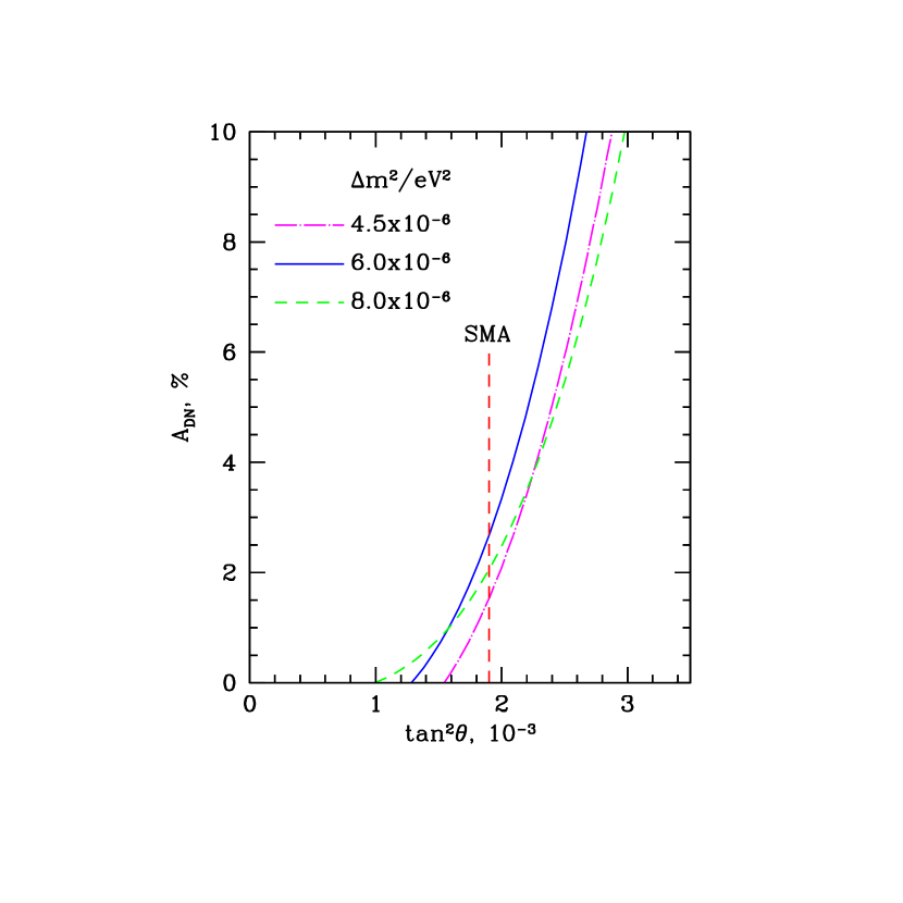
Figure 6: The dependence of the Day-Night asymmetry of the $CC-$event rate measured at SNO on $\tan^{2}\theta$ for different values of $\Delta m^{2}$. The oscillation parameters are taken from the SMA allowed region. The best fit value of $\tan^{2}\theta$ is marked by the vertical dotted line.

3). SMA solution. The dependence of the asymmetry on $\tan^{2}\theta$ for different values of $\Delta m^{2}$ is shown in Fig. 6. In the best fit point we get $A_{DN}^{SNO}=2.6\%$ and most of this asymmetry is collected from the “core” bin. The asymmetry increases fast with $\tan^{2}\theta$. In the $3\sigma$ allowed region it can be as large as 8%.

The SNO asymmetry is only slightly higher than the SK- asymmetry: $A_{DN}^{SK}=2.4\%$. In the SMA range due to strong dependence of the survival probability on energy the relation between the SNO and SK asymmetries is more complicated than in Eq. (19).

4.2 Spectrum distortion

As follows from previous studies [39, 40, 31], in general the sensitivity of the SNO measurements to the energy spectrum distortion is higher than the sensitivity of SuperKamiokande due to better correlation of the neutrino and the (produced) electron energies. However, the present statistics in SNO is much lower than in SK, and the statistical errors are more than 2 times larger (in the range 8 - 10 MeV we get 10 -12 % at SNO as compared with 4 - 5 % at SK).

In our analysis we do not use the spectral information from SNO. Instead, we present here a qualitative discussion comparing the present SNO data with predicted spectra from different solutions. This allows us to evaluate significance of the present and forthcoming SNO results.

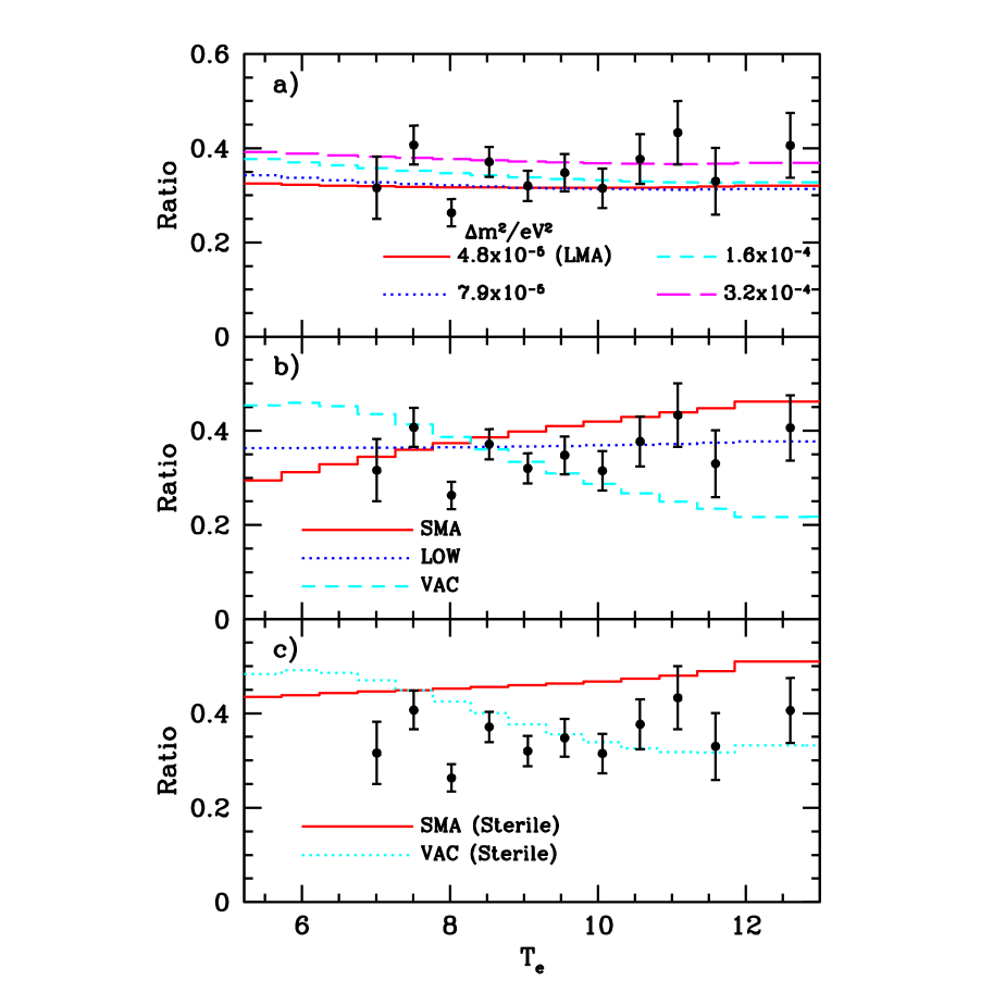
Figure 7: The recoil electron energy spectra of the $CC-$events in SNO for global solutions of the solar neutrino problem. Shown are the ratio of the number of events with and without conversion as a function of the electron kinetic energy. a). The spectra in the LMA solution region for different values of $\Delta m^{2}$ and $\tan^{2}\theta=0.35$. b). Spectra for the best fit points of the SMA, LOW and VAC (active) solutions. c). Spectra for the best fit points of the SMA(sterile) and VAC(sterile) solutions. Shown also in all panels is the SNO experimental data.

In Fig. 7 we show the expected spectra of events at SNO for several values of the oscillation parameters in the LMA region. In the high energy part of the spectrum the distortion is due to the earth regeneration effect as well as contribution of the $hep-$ neutrino flux. However, for $\Delta m^{2}\leq(4-5)\cdot 10^{-5}$ eV² the regeneration effect is small and the turn up at $E>11$ MeV is due to increased ($f_{hep}=5$) flux of the $hep-$neutrinos. The turn up of the spectrum at low energies is the effect of the adiabatic edge of the suppression pit. Recall that the ratio of the event rate with oscillations to the event rate with no oscillations is determined by the product of the survival probability times the factor $f_{B}$: $R_{CC}\propto f_{B}(\Delta m^{2})\bar{P}(\Delta m^{2})$. With increase of $\Delta m^{2}$ spectrum shifts to the adiabatic edge; for $\Delta m^{2}<10^{-5}$ eV² the probability can be written as

$$\bar{P}\approx(\sin^{2}\theta+f_{reg}+A),$$

where $A$ is the correction due to adiabatic edge and it is proportional to the first moment $\delta T$:

$$A\propto\delta T\propto\cos 2\theta\left(\frac{\Delta m^{2}}{E}\right)^{2}$$ (22)

(see Appendix of [17] for more details). The factor $\cos 2\theta$ accounts for the disappearance of the distortion when the mixing approaches maximal value. With increasing $\Delta m^{2}$ the size of the turn up and the distortion of the spectrum (first moment) increase as $(\Delta m^{2})^{2}$. Notice that at the same time $f_{B}$ decreases to compensate for a total increase of the survival probability. The distortion reaches a maximum at $\Delta m^{2}\sim 1.5\cdot 10^{-4}$ eV² when the boron neutrino spectrum is in the middle of the adiabatic edge. With further increase of $\Delta m^{2}$, the spectrum shifts out of the suppression pit and the distortion decreases. For $\Delta m^{2}>3\cdot 10^{-4}$ eV² the spectrum is in the range where the probability is determined basically by the averaged vacuum oscillations: $P=1-\sin^{2}2\theta/2$ and does not depend on the neutrino energy. Notice that the distortion of the spectrum weakens due to integration over neutrino energy and folding with the energy resolution function. Moreover, the SNO sensitivity to the distortion at low energies is weakened by the fast decrease of the cross-section with energy.

The curves shown in Fig. 7a illustrate this behavior of the spectrum. The short dashed line corresponds to near maximal distortion. As follows from the figure it will be very difficult to establish the distortion expected from the LMA solution with SNO. One needs to measure the spectrum down to $\sim 5$ MeV and to increase substantially the statistics. Thus, the prediction for SNO is that no significant distortion should be seen in forthcoming measurements.

In Fig. 7b we show the expected spectra of events at SNO in the best fit points of the LOW, SMA and VAC(active) solutions. The correlated systematic errors (mainly due to the error in the absolute energy scale calibration) are not shown here. These errors can affect the conclusions from the fit to the spectrum, making the spectrum appear flatter.

In the best fit point of the LOW solution the Earth regeneration effect on the shape of the spectrum is small. The weak positive slope (positive shift of the first moment) is due to the effect of the adiabaticity violation (non-adiabatic edge of the suppression pit). The slope increases with decreasing $\tan^{2}\theta$ as well as $\Delta m^{2}$ (for some analytical studies see [17]). It will be difficult to establish this distortion with SNO.

For the VAC (active) solution with low $\Delta m^{2}$, Eq. (13), one predicts maximum of the ratio $R_{CC}$ at $E\sim 6$ MeV. It corresponds to the first oscillation maximum of the survival probability. The ratio decreases with increase of energy and at $E>11$ MeV the distortion flattens due to contribution of the $hep-$neutrino flux. Thus, negative shift of the first moment (slope) is expected. As follows from the figure, the distortion is at the border of sensitivity of already present SNO data (correlated systematic errors can partly improve an agreement between the data and the predictions). Further increase of statistics and especially measurements of the spectrum at lower energies will be crucial for discrimination of the solution. Notice that the oscillation parameters are well fixed by the SK spectrum, and no freedom exists, e.g., to change the distortion by varying $\Delta m^{2}$. In particular, the position of the maximum at $E\sim 6$ MeV is immediately determined by the maximum in the SK spectrum at 8 MeV. The distortion can be identified by comparison of the averaged ratio $R_{CC}$ at low and high energies: $R_{CC}(<9~{}{\rm MeV})$ and $R_{CC}(>9~{}{\rm MeV})$.

Similar distortion is expected for the VAC(sterile) solution, see Fig.7c. For VAC (active) with high $\Delta m^{2}$ (see Eq. (14)) one expects flat distribution at low energies due to strong averaging effect and a bump at high energies $E>12$ MeV.

For the SMA (active) solution there is a strong positive shift of the first moment (slope). Correlated systematic errors improve the agreement with the experimental data. The present SNO data can already have some impact on this solution. The allowed region will drift to smaller mixing angles where the distortion is weaker. The best fit boron flux should decrease in order to compensate for the increase of the survival probability.

For SMA(sterile) the distortion is very weak, as a consequence of very small mixing angle. However for this solution the predicted spectrum is systematically above the experimental points which corresponds to $3.3\sigma$ higher total rate.

In conclusion, the present SNO spectral data further favor the LMA and LOW solutions. However, it will be difficult to establish with SNO the weak spectral distortions expected for these solutions. At the same time the SNO measurements can be sensitive to strong distortion of the spectrum predicted by already disfavored solutions such as VAC and SMA.

4.3 NC/CC ratio

The reduced neutral current event rate [NC] is defined as the ratio of the rates with and without oscillations: $[{\rm NC}]\equiv N_{NC}/N_{NC}^{SSM}$. Similarly, the reduced rate of the charged current event rate equals $[{\rm CC}]\equiv N_{CC}/N_{CC}^{SSM}$. We have calculated the ratio of the NC and CC reduced rates, [NC]/[CC], for global solutions found from the free flux fit.

For the active neutrino conversion the ratio equals

$$\frac{\rm NC}{\rm CC}=\frac{1}{\bar{P}}\approx\frac{f_{B}}{R_{SNO}},$$ (23)

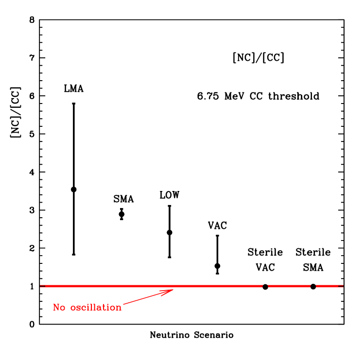
Figure 8: The ratio of the reduced NC - event rate to the reduced CC- event rate. The circles give values of [NC]/[CC] in the best fit points of the global solutions. The error bars show the prediction intervals of [NC]/[CC] which correspond to the $3\sigma$ allowed regions of global solutions.

where $\bar{P}$ is the effective (averaged) survival probability of the electron neutrinos. In the best fit points, using results for $f_{B}$ and $R_{SNO}$ from the Tables 1 and 5, we find [NC]/[CC] $=3.5$ (LMA), 2.4 (LOW), 2.8 (SMA), 1.5 (VAC), $\approx 1$ (Just-so²) in agreement with results of numerical calculations (see fig. 8).

For the sterile solutions we have:

$$\frac{\rm[NC]}{\rm[CC]}=\frac{\bar{P}_{NC}}{\bar{P}_{CC}},$$ (24)

where $\bar{P}_{NC}$ and $\bar{P}_{CC}$ are the effective survival probabilities for the NC and CC samples correspondingly. For the NC sample the energy threshold is about 2.2 MeV, so that ${P}_{NC}$ is averaged over larger interval than ${P}_{CC}$. As a consequence, the probabilities $\bar{P}_{CC}$ and $\bar{P}_{NC}$ are in general different.

Notice that the largest value of the ratio is expected for the LMA solution:

$$\frac{\rm[NC]}{\rm[CC]}=3.5^{+2.4}_{-1.7}~{}~{}~{}({\rm LMA})~{}.$$ (25)

Then rather close predictions follow from the SMA and LOW solutions. Smaller value is predicted for VAC. For sterile solutions the ratio is close to 1.

According to fig. 8, there is a significant overlap of the $3\sigma$ regions of predictions. However, measurements of the ratio with better than 20 % accuracy can significantly contribute to discrimination of the solutions.

4.4 BOREXINO rate

For global solutions we have calculated the reduced event rate in the BOREXINO experiment [42], $R_{borexino}\equiv N_{osc}/N_{SSM}$, where $N_{osc}$ and $N_{SSM}$ are the expected rates with and without neutrino conversion. We averaged the effect over the year.

The rate can be estimated as $R_{borexino}=\bar{P}_{Be}(1-r)+r$, where $\bar{P}_{Be}$ is the averaged survival probability for the ⁷Be- neutrino line. The probability $\bar{P}_{Be}$ has been calculated for the oscillation parameters from the $3\sigma$ allowed regions of solutions found from the free flux analysis. $r$ is the ratio of cross-sections of the $\nu_{\mu}e-$ and $\nu_{e}e-$ scattering at the the beryllium line. We have used the neutrino-electron scattering cross-sections from Ref. [43].

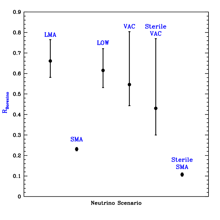
Figure 9: The reduced event rate in the BOREXINO experiment. The circles give values of $R_{borexino}$ in the best fit points of the global solutions. The error bars show the prediction intervals which correspond to the $3\sigma$ allowed regions of global solutions.

The results of calculations for six global solutions are shown in the Fig. 9. The rate is suppressed for the solutions. In particular, for the LMA solution we get

$$R_{borexino}=0.66^{+0.11}_{-0.08}~{}~{}~{}~{}({\rm LMA}).$$

Similar suppression is expected for the LOW. The VAC solutions predict stronger suppression, the lowest rate is expected for SMA. Notice that the range of predictions for SMA is very small due to smallness of the allowed region itself.

There is a significant overlap of the predicted intervars for LMA, LOW and VAC. Therefore, it will be difficult to discriminate among these solutions using just total rate measurements. However, Borexino has other capabilities, e.g. it can detect strong day-night effect in the case of the LOW solutions [44], whereas strong seasonal variations are expected if QVO or VAC solution is realized [45].

5 Conclusions

We have performed a global analysis of the solar neutrino data including the charged current event rate measured by SNO. We tested the robustness of the global solutions by modifying the analysis. The quality of the fit was checked by construction of the pull-off diagrams.

We find that the LMA solution with parameters in the range $\Delta m^{2}\sim(4-5)\cdot 10^{-5}$ eV² and $\tan^{2}\theta=0.35-0.40$ gives the best fit to the data. Moreover, the solution reproduces the flat spectrum of recoil electrons in SK and gives very good description of the rates and of the Day-Night asymmetry. It is in a very good agreement with SSM fluxes of the boron ($f_{B}=1.10-1.13$) and $hep-$neutrinos. The values of the oscillation parameters and the goodness of the fit are stable with respect to variations of the analysis.

The LOW solution appears at 90 % C.L. with respect to the best fit point in the LMA range. It gives good fit to the SK spectral data, but rather poor fit to the rates: it predicts larger than measured $Ar-$production rate and smaller than measured $Ge-$production rate.

The VAC solution has high goodness of the global fit due to a very good description of the day and the night spectra measured by SK. It has, however, problems with other criteria. The solution requires strong deviation of the boron and $hep-$fluxes from their SSM values. The fit becomes substantially worse when SSM restrictions are applied. The solution shows strong deviations in the pull-off diagram (especially for the SuperKamiokande rate and the $Ar-$production rate). The analysis of the rates only selects a different point in the oscillation parameter space.

The SMA appears at about $3\sigma$ C.L. level with respect to the best global solution in the LMA range. It gives bad fit of the recoil electron energy spectrum and also the fit of the rates is rather poor.

The best sterile solution is VAC(sterile) with $\Delta m^{2}=1.4\cdot 10^{-10}$ eV². It is the only sterile solution accepted at lower than $3\sigma$ C.L. in the free flux analysis. This solution, however, has serious problems with other tests. Similarly to VAC(active) the solution requires strong deviation of the boron and $hep-$ fluxes from their SSM values. The fit becomes substantially worse when SSM restrictions are applied. The solution shows strong deviations in the pull-off diagram: in particular, the $\nu e-$ event rate is about $3\sigma$ below the SK rate, the $Ar-$production rate is $2.4\sigma$ higher than the Homestake result. The analysis of the rate only selects a different point in the oscillation parameter space. Significant distortion of the energy spectrum is expected. Appearance of the VAC solutions (both active and sterile) in the global fit is related to a small spread of the experimental points in the SK spectrum. These solutions can describe rather precisely the bump at 7 - 8 MeV and the dip at 11 - 12 MeV.

Maximal mixing is allowed at $3\sigma$ level in the LMA region and at 99 % C.L. in the LOW and quasivacuum oscillation regions.

Measurements of the D-N asymmetry will provide strong discrimination among the solutions. In the best fit range of the LMA solution the asymmetry in SNO is $A_{DN}^{SNO}\simeq(7-8)\%$, and in the $3\sigma$ allowed region it can reach 15 - 20 %. In the LOW region one expects smaller asymmetry: in the best fit point $A_{DN}^{SNO}\simeq(2-3)\%$, although in the $3\sigma$ allowed region it can be as large as 10 - 12 %. For the SMA solution the asymmetry is $A_{DN}^{SNO}\leq 3\%$. The predicted SMA zenith angle distribution is not supported by SK data.

Clearly, observation of a large D-N asymmetry $A_{DN}^{SNO}>5\%$ will favor the LMA solution. It will strongly disfavor the SMA solution, and exclude solutions based on vacuum oscillations (VAC, QVO and and Just-so²). Furthermore, this result will strongly restrict LMA to lower $\Delta m^{2}$. Even with existing statistics (expected error is 3 - 4 %) any SNO result on the D-N asymmetry will be of physical importance excluding some solutions or further restricting the allowed regions.

Significant distortion of the boron neutrino spectrum is expected for SMA and VAC solutions and already the present data can affect them. The VAC solution predicts the bump at 6 MeV and the dip at 11 MeV in the dependence of the $R_{CC}$ on energy. In the case of LMA solution turn up of the spectrum at low energies is expected which will be rather difficult to observe with SNO. For LMA and LOW one expects practically no distortion in future SNO measurements.

Important discrimination among solutions can be done using precise determination of the [NC]/[CC] ratio.

With forthcoming SNO data, we have a chance to make further major step in identification of the solution of the solar neutrino problem.

References

- [1] Q. R. Ahmad et al., SNO collaboration, nucl-ex/0106015.
- [2] A. B. McDonald, Proc. of the 19th Int. Conf. on Neutrino Physics and Astrophysics, Neutrino 2000 , Sudbury, Canada 2000, Nucl. Phys. B (Proc. Suppl.) 91 (2001) 21.
- [3] S. Fukuda et al. (SuperKamiokande collaboration) hep-ex/0103032.
- [4] J. N. Bahcall, hep-ph/0108147, hep-ph/0108148; V. Berezinsky hep-ph/0108166.
- [5] J. N. Bahcall, P.I. Krastev, A. Yu. Smirnov, JHEP 5 (2001) 15.
- [6] See previous analysis of this type: Waikwok Kwong, S. P. Rosen, Phys. Rev. D 54 (1996) 2043; F.L. Villante, G. Fiorentini, E. Lisi, Phys. Rev. D59 (1999) 013006; J. N. Bahcall, P.I. Krastev, A. Yu. Smirnov, Phys. Lett. B 477 (2000) 401.
- [7] V. Barger, D. Marfatia and K. Whisnant, hep-ph/0106207.
- [8] G.L. Fogli, E. Lisi, D. Montanino and A. Palazzo, hep-ph/0106247.
- [9] J. N. Bahcall, M. C. Gonzalez-Garcia, Carlos Pena-Garay, hep-ph/0106258.
- [10] A. Bandyopadhyay, S Choubey, S. Goswami, K. Kar, hep-ph/0106264.
- [11] A. de Gouvea and C. Pena-Garay, hep-ph/0107186.
- [12] R. Barbieri, A. Strumia, hep-ph/0011307, v4 (July 2001).
- [13] C. Giunti, hep-ph/0107310.
- [14] V. Berezinsky M. Lissia, hep-ph/0108108.
- [15] J.N. Bahcall, P.I. Krastev and A.Yu. Smirnov, Phys. Rev. D58 096016 (1998).
- [16] J. N. Bahcall, P.I. Krastev, A. Yu. Smirnov, Phys. Rev. D 62 (2000) 093004.
- [17] J. N. Bahcall, P.I. Krastev, A. Yu. Smirnov, Phys. Rev. D 63 (2001) 053012.
- [18] B. T. Cleveland et al Astroph. J. 496 (1998) 505; K. Lande et al, in Neutrino 2000 [2], p.50.
- [19] V. Gavrin, (SAGE collaboration) Proc. of the 19th Int. Conference on Neutrino Physics and Astrophysics, Neutrino 2000 , Sudbury, Canada, June 2000, Nucl. Phys. B (Proc. Suppl.) 91 (2001) 36.
- [20] W. Hampel et al. (GALLEX Collaboration) Phys. Lett. B 447 (1999) 127.
- [21] M. Altmann et al. (GNO Collaboration) Phys. Lett. B 490 (2000) 16; E. Bellotti et al. Proc. of the XIX Int. Conference on Neutrino Physics and Astrophysics, Neutrino 2000, Sudbury, Canada 2000, Nucl. Phys. B (Proc. Suppl.) 91 (2001) 44.
- [22] J. N. Bahcall, M.H. Pinsonneault and S. Basu, Astrophys. J. 555 (2001)990.
- [23] P. I. Krastev and A. Yu. Smirnov, Phys. Lett. B338 (1994) 282.
- [24] L. E. Marcucci et al., Phys. Rev. C63 (2001) 015801; T.-S. Park, et al., hep-ph/0107012 and references therein.
- [25] P. Creminelli, G. Signorelli, A. Strumia, JHEP 0105 (2001) 052, hep-ph/0103179.
- [26] J. N. Bahcall, P.I. Krastev, A. Yu. Smirnov, Phys. Rev. D60 (1999) 093001.
- [27] S. Geer, Phys. Rev. D57 (1998) 6989.
- [28] CHOOZ Collaboration, M. Apollonio et al., Phys.Lett. B420, 397 (1998).
- [29] S. P. Mikheyev and A. Yu. Smirnov, ’86 Massive Neutrinos in Astrophysics and in Particle Physics Proc. of the 6th Moriond Workshop, edit by O. Fackler and J. Tran Thanh Van (Edition Frontiers Gif-sur-Yvette, 1986) p. 355; A. J. Baltz and J. Weneser, Phys. Rev. D50 5971 (1994), ibid D51 (1994) 3960; E. Lisi, D. Montanino, Phys. Rev. D56 (1997) 1792; J. M. Gelb, Wai-kwok Kwong, S. P. Rosen, Phys. Rev. Lett. 78 (1997) 2296.
- [30] S. T. Petcov, Phys. Lett. B434 (1998); E. Kh. Akhmedov, Nucl. Phys. B 538 (1999) 25; M. V. Chizhov and S. T. Petcov, Phys. Rev. Lett. 83 (1999) 1096.
- [31] K. S. Babu, Q. Y. Liu, A. Yu. Smirnov, Phys. Rev. D57 (1998) 5825.
- [32] M. C. Gonzalez-Garcia, C. Pena-Garay, Y. Nir, A. Yu. Smirnov, Phys. Rev. D63 (2001) 013007.
- [33] G. Dvali and A. Yu. Smirnov, Nucl. Phys. B563 (1999) 63.
- [34] A. Lukas, P. Ramond, A. Romanino, G. G. Ross, JHEP 0104:010, 2001; D.O. Caldwell, R.N. Mohapatra, S.J. Yellin, hep-ph/0102279.
- [35] J. N. Bahcall and P. I. Krastev, Phys. Rev. C56 (1997) 2839.
- [36] M. Maris and S. T. Petcov, Phys. Rev. D62 (2000) 093006.
- [37] G. L. Fogli, E. Lisi, D. Montanino, A. Palazzo, hep-ph/0008012.
- [38] M. C. Gonzalez-Garcia, C. Pena-Garay, A. Yu. Smirnov, Phys. Rev. D63 (2001) 113004.
- [39] J. N. Bahcall and E. Lisi, Phys. Rev. D54 (1996) 5417.
- [40] J. N. Bahcall, P. I. Krastev and E. Lisi, Phys. Rev. C55 (1997) 494.
- [41] G. L. Fogli, E. Lisi and D. Montanino, Astropart. Phys. 9 (1998) 119.
- [42] BOREXINO Collaboration, G. Ranucci et al., 19th International Conference on Neutrino Physics and Astrophysics - Neutrino 2000, Sudbury, Ontario, Canada, 16-21 June 2000, Nucl. Phys. Proc. Suppl. 91 (2001) 58.
- [43] J. N. Bahcall, M. Kamionkowski, A. Sirlin, Phys. Rev. D51 (1995) 6146.
- [44] A.J. Baltz, J. Weneser, Phys. Rev. D50 (1994) 5971, Addendum-ibid. D51 (1995) 3960; for recent analysis see A. de Gouvea, A. Friedland, H. Murayama, JHEP 0103 (2001) 009; G.L. Fogli, E. Lisi, D. Montanino, A. Palazzo, Phys. Rev. D61 (2000) 073009.
- [45] For recent analysis see B. Faid, G.L. Fogli, E. Lisi, D. Montanino, Astropart. Phys., 10 (1999) 93; A. de Gouvea, A. Friedland, H. Murayama, Phys. Rev. D60 (1999) 093011.