Collective modes of color-flavor locked phase of dense QCD at finite temperature

Abstract

A detailed analysis of collective modes that couple to either vector or axial color currents in color-flavor locked phase of color superconducting dense quark matter at finite temperature is presented. Among the realm of collective modes, including the plasmons and the Nambu-Goldstone bosons, we also reveal the gapless Carlson-Goldman modes, resembling the scalar Nambu-Golstone bosons. These latter exist only in a close vicinity of the critical line. Their presence does not eliminate the Meissner effect, proving that the system remains in the color broken phase. The finite temperature properties of the plasmons and the Nambu-Goldstone bosons are also studied. In addition to the ordinary plasmon, we also reveal a “light” plasmon which has a narrow width and whose mass is of the order of the superconducting gap.

I Introduction

In the last few years much progress has been achieved in understanding the possible phases of quantum chromodynamics (QCD) at low temperatures and high densities. In particular it is expected that QCD at a sufficiently large density of quark matter possesses color superconducting phases [1, 2]. It is widely believed that one of color superconducting phases may exist even at moderate densities that characterize the matter at the cores of compact stars (i.e., at densities just a few times larger than the density of the ordinary nuclear matter). The value of the superconducting order parameter is likely to be of order $10$ to $100$ MeV [3, 4] (see also Refs. [5, 6, 7, 8, 9, 10, 11, 12, 13, 14] for estimates using the microscopic approach). These estimates of the order parameter are encouraging to seek for observable signatures from a color superconducting state inside compact stars [15]. While there are no many detailed studies in this direction yet, a couple of issues have already been addressed in Refs. [16, 17, 18], and some of their conclusions seem to be very promising.

At (asymptotically) large densities, the microscopic QCD becomes a weakly interacting theory [19]. This allows one to use analytical (although, non-perturbative) methods of quantum field theory for studying dense quark matter. At finite chemical potential $\mu$, non-interacting quarks should occupy all the states with momenta $|\vec{p}|<\mu$, thus, forming the Fermi surface. In a more realistic (weakly) interacting model, the attraction between quarks in the color-antitriplet channel leads to the famous Cooper instability. The latter is removed by a rearrangement of the ground state. As a result, in the case of the model with three quark flavors, the original gauge symmetry $SU(3)_{c}$ and the global chiral symmetry $SU(3)_{L}\times SU(3)_{R}$ break down to the global diagonal $SU(3)_{c+L+R}$ subgroup [20]. The corresponding phase is called the color-flavor locked (CFL) phase. Out of total sixteen candidates for Nambu-Goldstone (NG) bosons, eight are removed from the physical spectrum by the Higgs mechanism, providing masses to eight gluons. The other eight NG bosons show up as an octet (under the unbroken $SU(3)_{c+L+R}$) of physical particles. In addition, the global baryon number symmetry as well as the approximate $U(1)_{A}$ symmetry also get broken. As a result, an extra NG boson and a pseudo-NG boson appear in the low energy spectrum. These latter particles are both singlets under $SU(3)_{c+L+R}$.

The low energy effective action of the CFL phase was derived in Refs. [21, 22, 23, 24, 25], based on arguments of symmetry. Moreover, all parameters of the action were calculated in the limit of the asymptotically large chemical potential. The method of Refs. [21, 22, 23, 24, 25] is based on matching vacuum properties (such as vacuum energy and gluon screening) in the effective and microscopic theories. While being very powerful for many purposes, such a method is limited when it comes to determining the spectrum of bound states other than NG bosons. The other approach used to study (diquark) bound states is based on the Bethe-Salpeter (BS) equation [26]. (A simplified study of the BS equation was also considered in Ref. [27] and, for the case of two flavor dense QCD, in Ref. [28].)

In this paper, we study the spectrum of collective excitations in the CFL phase at finite temperature. To be more specific, we study only those collective modes that couple to the (vector and axial) color currents. The NG bosons and the massive plasmons are the examples of such modes. As we shall see, however, the plasmons and NG bosons do not exhaust all of the collective modes. In addition, we also predict the existence of the so-called Carlson-Goldman (CG) modes in the CFL phase of dense QCD (a short outline of this prediction was given in Ref. [29]). In ordinary superconductors, the CG modes were experimentally discovered long time ago [30]. These modes appear only in a close vicinity of the critical line. Their quantum numbers are the same as those of the scalar NG bosons that are removed from the physical spectrum by the Higgs mechanism. Because of this, the appearance of the CG modes might look like a revival of the NG bosons [31].

This paper is organized as follows. In Sec. II, we describe our model and introduce basic notations. Then, we present the general form of the effective action of the gluon field and discuss its most important properties in Sec. III. In Sec. IV, we give the explicit form of the finite temperature improved hard-dense loop expression for the polarization tensor and reveal its internal structure. Then, by making use of the polarization tensor, we derive the general form of the current-current correlation function in Sec. V. In the same section, we derive the gluon and the (order parameter) phase field propagators and check that their poles appear at the same locations as in the current-current correlation function. In Sec. VI, we present a general formalism for studying collective modes, coupled to vector (as well as axial) color currents. In Sec. VII, VIII and IX, we analyze the properties of the plasmons, the NG bosons and the gapless Carlson-Goldman modes, respectively. Sec. X deals with the Meissner effect in the color superconducting phase. We derive the penetration depth of a constant magnetic field, and show that the superconducting quark matter corresponds to the so-called Pippard limit everywhere in the superconducting part of the phase diagram except for a very small region in the vicinity of the critical temperature. We summarize our results in Sec. XI. Some useful notations and formulas are collected in Appendices B and A. In Appendix C, we present the general one-loop expression and the hard dense loop approximation of polarization tensor. The key integrals, used in the definition of the polarization tensor, are defined and approximately calculated in Appendices D and E.

II Model and notation

As we mentioned in Introduction, the original $SU(3)_{c}\times SU(3)_{L}\times SU(3)_{R}$ symmetry of massless QCD breaks down to the global diagonal $SU(3)_{c+L+R}$ subgroup in the CFL ground state of dense quark matter. The color condensate in the CFL phase is given by the vacuum expectation value of the following diquark (antidiquark) field [20]:

$$\langle 0|\left(\bar{\Psi}_{D}\right)^{a}_{i}\gamma^{5}\left(\Psi_{D}^{C}\right)^{b}_{j}|0\rangle=\kappa_{1}\delta^{a}_{i}\delta^{b}_{j}+\kappa_{2}\delta^{a}_{j}\delta^{b}_{i},$$ (1)

where $\Psi_{D}$ and $\Psi_{D}^{C}=C\bar{\Psi}^{T}_{D}$ are the Dirac spinor and its charge conjugate spinor, and $C$ is a unitary matrix that satisfies $C^{-1}\gamma_{\mu}C=-\gamma^{T}_{\mu}$ and $C=-C^{T}$. In the last expression, we explicitly displayed the flavor ($i,j=1,2,3$) and color ($a,b=1,2,3$) indices of the spinor fields. The complex scalar quantities $\kappa_{1}$ and $\kappa_{2}$ are determined by dynamics. Throughout the paper, we follow the notation of Ref. [26] as close as possible.

It is convenient to introduce the color-flavor locked Weyl spinors ( octets and singlets under $SU(3)_{c+L}$ and $SU(3)_{c+R}$, respectively) to replace the ordinary Dirac spinors,

$$\psi^{A}=\frac{1}{\sqrt{2}}{\cal P}_{+}(\Psi_{D})^{~{}i}_{a}\left(\lambda^{A}\right)_{i}^{~{}a}, \psi=\frac{1}{\sqrt{3}}{\cal P}_{+}(\Psi_{D})^{~{}i}_{a}\delta_{i}^{~{}a},$$ (3)

$$\tilde{\psi}^{A}=\frac{1}{\sqrt{2}}{\cal P}_{-}(\Psi_{D}^{C})_{j}^{~{}b}\left(\lambda^{A}\right)_{b}^{~{}j}, \tilde{\psi}=\frac{1}{\sqrt{3}}{\cal P}_{-}(\Psi_{D}^{C})_{j}^{~{}b}\delta_{b}^{~{}j},$$ (4)

$$\phi^{A}=\frac{1}{\sqrt{2}}{\cal P}_{-}(\Psi_{D})^{~{}i}_{a}\left(\lambda^{A}\right)_{i}^{~{}a}, \phi=\frac{1}{\sqrt{3}}{\cal P}_{-}(\Psi_{D})^{~{}i}_{a}\delta_{i}^{~{}a},$$ (5)

$$\tilde{\phi}^{A}=\frac{1}{\sqrt{2}}{\cal P}_{+}(\Psi_{D}^{C})_{j}^{~{}b}\left(\lambda^{A}\right)_{b}^{~{}j}, \tilde{\phi}=\frac{1}{\sqrt{3}}{\cal P}_{+}(\Psi_{D}^{C})_{j}^{~{}b}\delta_{b}^{~{}j},$$ (6)

where $A=1,\ldots,8$, and the sum over repeated indices is understood. Tilde denotes the charge conjugate spinors. Also, we use the conventional definition of the left- and right-handed projectors, ${\cal P}_{\pm}=(1\pm\gamma^{5})/2$.

In the new notation, the non-zero order parameters $\kappa_{1}$ and $\kappa_{2}$, as defined in Eq. (1), are related to the following (singlet under the color-flavor locked residual symmetry) vacuum expectation values:

$$\langle 0|\bar{\psi}\tilde{\psi}|0\rangle=-\langle 0|\bar{\phi}\tilde{\phi}|0\rangle=-\frac{1}{2}\left(3\kappa_{1}+\kappa_{2}\right),$$ (8)

$$\langle 0|\bar{\psi}^{A}\tilde{\psi}^{B}|0\rangle=-\langle 0|\bar{\phi}^{A}\tilde{\phi}^{B}|0\rangle=-\frac{1}{2}\delta^{AB}\kappa_{2}.$$ (9)

In general, the order parameters $\kappa_{1}$ and $\kappa_{2}$ are not independent. The details of the pairing dynamics should define a specific relation between the values of $\kappa_{1}$ and $\kappa_{2}$. The value of their ratio, in its turn, defines a specific alignment of the order parameter. The analysis of the SD equation in phenomenological four-fermion models [20], as well as in the microscopic QCD theory [12, 13], shows that the order parameter is dominated by the antitriplet-antitriplet contribution ($\kappa_{1}=-\kappa_{2}$). While the sextet-sextet admixture ($\kappa_{1}=\kappa_{2}$) is small, it is never exactly zero. In fact, the latter does not break any additional symmetries [20], and, for that reason alone, it cannot be excluded. In our analysis, we restrict ourselves to the case of a pure antitriplet-antitriplet order parameter. We do this simply for the purpose of convenience of presentation. The modification of our analysis to the case with a nonzero sextet-sextet order parameter is straightforward. In particular, it would only require to slightly change the ratio of the gaps for the quasiparticle in the octet and singlet channels (see below).

The value of the order parameter in the CFL phase at zero temperature was estimated in Refs. [20, 12, 13], using phenomenological four-fermion as well as microscopic models [see Refs. [5, 6, 7, 8, 9, 10, 11], dealing with the two flavor case]. While the exact value remains uncertain, it can be as large as $100$ MeV. The temperature dependence of the diquark order parameter is essentially the same as that in the standard BCS theory of superconductivity [14]. Notice that the Meissner effect was neglected in the analysis of Ref. [14]. However, the recent result of Ref. [32] suggests that such an approximation is justified.

For completeness of presentation, we note that the inverse form of the relations in Eq. (II) reads

$$(\Psi_{D})_{a}^{~{}i}=\frac{1}{\sqrt{2}}\left(\psi^{A}+\phi^{A}\right)\left(\lambda^{A}\right)_{a}^{~{}i}+\frac{1}{\sqrt{3}}\left(\psi+\phi\right)\delta_{a}^{~{}i}$$ (11)

$$(\Psi_{D}^{C})_{j}^{~{}b}=\frac{1}{\sqrt{2}}\left(\tilde{\psi}^{A}+\tilde{\phi}^{A}\right)\left(\lambda^{A}\right)_{j}^{~{}b}+\frac{1}{\sqrt{3}}\left(\tilde{\psi}+\tilde{\phi}\right)\delta_{j}^{~{}b}.$$ (12)

Because the quarks in the color broken phase acquire a nonvanishing Majorana mass, it is also useful to introduce the left-handed and right-handed Majorana spinors,

$$\Psi=\psi+\tilde{\psi}, \Psi^{A}=\psi^{A}+\tilde{\psi}^{A},$$ (14)

$$\Phi=\phi+\tilde{\phi}, \Phi^{A}=\phi^{A}+\tilde{\phi}^{A},$$ (15)

respectively. Then, in the CFL phase, the dynamically generated Majorana mass contribution takes a simple diagonal form,

$${\cal L}_{\Delta} = \frac{1}{2}\bar{\Psi}\left(2\Delta{\cal P}_{-}+2\tilde{\Delta}{\cal P}_{+}\right)\Psi-\frac{1}{2}\bar{\Psi}^{A}\left(\Delta{\cal P}_{-}+\tilde{\Delta}{\cal P}_{+}\right)\Psi^{A}$$ (16)

$$+ \frac{1}{2}\bar{\Phi}\left(2\Delta{\cal P}_{+}+2\tilde{\Delta}{\cal P}_{-}\right)\Phi-\frac{1}{2}\bar{\Phi}^{A}\left(\Delta{\cal P}_{+}+\tilde{\Delta}{\cal P}_{-}\right)\Phi^{A}.$$ (17)

Here $\Delta=\Delta^{+}_{T}\Lambda^{+}_{p}+\Delta^{-}_{T}\Lambda^{-}_{p}$ and $\tilde{\Delta}=\gamma^{0}\Delta^{\dagger}\gamma^{0}$, and the quark “on-shell” projectors are

$$\Lambda_{p}^{\pm}=\frac{1}{2}\left(1\pm\frac{\vec{\alpha}\cdot\vec{p}}{|\vec{p}|}\right),\quad\vec{\alpha}=\gamma^{0}\vec{\gamma}.$$ (18)

Notice that the absolute value of the Majorana mass in Eq. (17) in the singlet channel is twice as large as the that in the octet channel. Also, the signs of those mass terms are opposite. Such a choice [see Eq. (II)] corresponds to the assumption of a pure antitriplet-antitriplet color-flavor locked order parameter ($\kappa_{1}=-\kappa_{2}$).

By making use of the Majorana spinors in Eq. (II), the QCD action reads

$${\cal L}_{QCD} = \frac{1}{2}\bar{\Psi}\left(\not{\!p}+\mu\gamma^{0}\gamma^{5}\right)\Psi+\frac{1}{2}\bar{\Psi}^{A}\left(\not{\!p}+\mu\gamma^{0}\gamma^{5}\right)\Psi^{A}+\frac{1}{2}\bar{\Phi}\left(\not{\!p}-\mu\gamma^{0}\gamma^{5}\right)\Phi+\frac{1}{2}\bar{\Phi}^{A}\left(\not{\!p}-\mu\gamma^{0}\gamma^{5}\right)\Phi^{A}$$ (21)

$$-\frac{1}{4}F_{\mu\nu}F^{\mu\nu}+\frac{g}{4}\bar{\Psi}^{B}A^{A}_{\mu}\gamma^{\mu}\left(d^{ABC}\gamma^{5}-if^{ABC}\right)\Psi^{C}+\frac{g}{2\sqrt{6}}A^{A}_{\mu}\left(\bar{\Psi}\gamma^{\mu}\gamma^{5}\Psi^{A}+\bar{\Psi}^{A}\gamma^{\mu}\gamma^{5}\Psi\right)$$

$$-\frac{g}{4}\bar{\Phi}^{B}A^{A}_{\mu}\gamma^{\mu}\left(d^{ABC}\gamma^{5}+if^{ABC}\right)\Phi^{C}-\frac{g}{2\sqrt{6}}A^{A}_{\mu}\left(\bar{\Phi}\gamma^{\mu}\gamma^{5}\Phi^{A}+\bar{\Phi}^{A}\gamma^{\mu}\gamma^{5}\Phi\right).$$

Here the structure constants $d^{ABC}$ and $f^{ABC}$ are defined by the anticommutation and commutation relations of the Gell-Mann matrices,

$$\left\{\lambda^{A},\lambda^{B}\right\} = \frac{4}{3}\delta^{AB}+2d^{ABC}\lambda^{C},$$ (22)

$$\left[\lambda^{A},\lambda^{B}\right] = 2if^{ABC}\lambda^{C}.$$ (23)

By making use of the microscopic action in Eq. (21), we could derive the well known Schwinger-Dyson equation for the quark propagator in the HDL improved, ladder approximation [12]. Its solution reveals a dynamical generation of the Majorana quark masses. Such masses could be incorporated in the low energy quark action by the contribution ${\cal L}_{\Delta}$, presented in Eq. (17).

In this paper, we are primarily interested in studying the properties of the collective modes at the non-perturbative vacuum in which the quarks have the Majorana masses. A specific mechanism of the mass generation is irrelevant for us here. Therefore, we could use the Hartree-Fock approach in our analysis. In particular, we add and subtract the mass term ${\cal L}_{\Delta}$ to the microscopic action in Eq. (21). Then, we treat one of such terms as a part of the free quark propagator, while the other one as an interaction term. In this approach, a special care should be taken to preserve the gauge invariance of the model. This is because the Majorana mass term in Eq. (17) acquires phase factors under a general gauge transformation, and thus, it is not gauge invariant. To avoid the difficulty, it is convenient to consider the phases of the order parameter $\Delta$ as quantum fields restoring the gauge invariance of the model.

By taking into account the structure of the dynamically generated mass terms in Eq. (17), we arrive at the following quark propagators in the CFL phase,

$$S_{1}(p) = i\frac{\gamma^{0}(p_{0}+\epsilon_{p}^{+})-2\Delta^{+}_{T}}{p_{0}^{2}-(\epsilon_{p}^{+})^{2}-4|\Delta^{+}_{T}|^{2}}\Lambda_{p}^{-}{\cal P}_{+}+i\frac{\gamma^{0}(p_{0}-\epsilon_{p}^{+})-2(\Delta^{+}_{T})^{*}}{p_{0}^{2}-(\epsilon_{p}^{+})^{2}-4|\Delta^{+}_{T}|^{2}}\Lambda_{p}^{+}{\cal P}_{-}$$ (24)

$$+ i\frac{\gamma^{0}(p_{0}-\epsilon_{p}^{-})-2\Delta^{-}_{T}}{p_{0}^{2}-(\epsilon_{p}^{-})^{2}-4|\Delta^{-}_{T}|^{2}}\Lambda_{p}^{+}{\cal P}_{+}+i\frac{\gamma^{0}(p_{0}+\epsilon_{p}^{-})-2(\Delta^{-}_{T})^{*}}{p_{0}^{2}-(\epsilon_{p}^{-})^{2}-4|\Delta^{-}_{T}|^{2}}\Lambda_{p}^{-}{\cal P}_{-},$$ (25)

$$S_{8}^{AB}(p)\equiv\delta^{AB}S_{8}(p) = i\delta^{AB}\left(\frac{\gamma^{0}(p_{0}+\epsilon_{p}^{+})+\Delta^{+}_{T}}{p_{0}^{2}-(\epsilon_{p}^{+})^{2}-|\Delta^{+}_{T}|^{2}}\Lambda_{p}^{-}{\cal P}_{+}+\frac{\gamma^{0}(p_{0}-\epsilon_{p}^{+})+(\Delta^{+}_{T})^{*}}{p_{0}^{2}-(\epsilon_{p}^{+})^{2}-|\Delta^{+}_{T}|^{2}}\Lambda_{p}^{+}{\cal P}_{-}\right.$$ (26)

$$+ \left.\frac{\gamma^{0}(p_{0}-\epsilon_{p}^{-})+\Delta^{-}_{T}}{p_{0}^{2}-(\epsilon_{p}^{-})^{2}-|\Delta^{-}_{T}|^{2}}\Lambda_{p}^{+}{\cal P}_{+}+\frac{\gamma^{0}(p_{0}+\epsilon_{p}^{-})+(\Delta^{-}_{T})^{*}}{p_{0}^{2}-(\epsilon_{p}^{-})^{2}-|\Delta^{-}_{T}|^{2}}\Lambda_{p}^{-}{\cal P}_{-}\right),$$ (27)

for the left-handed fields. Similar expressions could also be written for the right-handed fields (the latter are obtained from the above expressions by the formal exchange of ${\cal P}_{-}$ and ${\cal P}_{+}$). In the last two equations, we used the following notation: $\epsilon_{p}^{\pm}=|\vec{p}|\pm\mu$. As is clear from the structure of the quark propagators above, the value of the gap in the one-particle quark spectrum is determined by $|\Delta^{-}_{T}|$. The so called antigap $|\Delta^{+}_{T}|$, on the other hand, has an obscure physical meaning because it can only be detected in the high energy ($q_{0}\gtrsim 2\mu$) antiparticle excitations. In what follows we shall use the shorthand notation $|\Delta_{T}|\equiv|\Delta^{-}_{T}|$ that should not create any confusion.

III Effective action of gluons

In this paper, we are mostly interested in collective modes, coupled to the (vector and axial) color currents. In the pursuit of a model independent treatment, we find it advantageous to start our consideration with the effective action, obtained by integrating out the quark degrees of freedom. Such an action could be easily derived in a wide class of four-fermion models of dense quark matter (in the weakly coupled regime). As one could check, the effective Lagrangian density for the gluon field should have the following general structure:

$${\cal L}_{g,\phi} = -\frac{1}{2}A^{A,\mu}_{-q}i\left[{\cal D}^{(0)}(q)\right]^{-1}_{\mu\nu}A^{A,\nu}_{q}-\frac{1}{2}\left[A^{A,\mu}_{-q}-iq^{\mu}\phi^{A}_{-q}\right]\Pi_{\mu\nu}(q)\left[A^{A,\nu}_{q}+iq^{\nu}\phi^{A}_{q}\right]+\ldots,$$ (28)

with the ellipsis denoting the interactions terms. Note that the presence of the phase field octet $\phi^{A}_{q}$ in the last expression is very important for preserving the gauge invariance of the model. Under a gauge transformation, the phase $\phi^{A}_{q}$ in Eq. (28) shifts so that it exactly compensates the transformation of the gluon field. Here we consider only infinitesimally small gauge transformations. In general, the gauge transformation of $\phi^{A}_{q}$ field is not a simple shift. However, it is always true that its transformation exactly compensates the transformation of the gluon field.

The derivation of the effective Lagrangian density (28) in dense QCD is not an easy task. In principle, one should start by integrating out the high energy gluons which, as is known from Refs. [5, 6, 7, 8, 9, 10, 11, 12, 13, 14], play the dominant role in the dynamical generation of the gap. As a result of the integration, a new 4-fermion interaction term would be produced in the action. This latter could be treated by introducing the quantum Hubbard-Stratonovich composite field $\hat{\Delta}$ with the quantum numbers of the color superconducting condensate. The effective Lagrangian density in Eq. (28), then, is given by integrating out the quark degrees of freedom in the mean field approximation in which the vacuum expectation value of the composite field is fixed constant. This constant is identified with the value of the order parameter, $\langle\hat{\Delta}\rangle\equiv\Delta$. The fields $\phi^{A}$ are the phase fields of the composite field $\hat{\Delta}$ that correspond to the (would be) NG bosons.

While the microscopic theory of dense quark matter may truly be non-perturbative, the dynamics of gluon quasiparticles, given by the Lagrangian density in Eq. (28), could still be weakly interacting. This is known to be the case at least in the limit of asymptotically large quark densities. In this case, the explicit expression for the polarization tensor $\Pi_{\mu\nu}$ can be derived. Moreover, it is likely that the theory defined by Eq. (28) is applicable even at realistic densities existing at the cores of compact stars (despite the fact that the derivation of Eq. (28) fails at low density). This is because, in the case of weakly coupled gluons, the expression in Eq. (28) is the only possible quadratic expression consistent with the $SU(3)_{c}$ color gauge symmetry.

In what follows, we use the simplest approximation for the polarization tensor $\Pi_{\mu\nu}$ given by the improved hard dense loop (IHDL) approximation. Here “improved” indicates that the effect of the nonzero values of quark gaps are taken into account in the calculation of loop diagrams. The formal expression of such tensor was presented in Ref. [34]. The zero temperature limit was also considered in Ref. [24]. Below, we present some other limits which has not been analyzed previously. In our notation, the explicit form of the (left-handed contribution of) IHDL polarization tensor (in the Matsubara formalism) reads

$$\Pi_{L,\mu\nu}(i\Omega_{m},q) = -\frac{g^{2}T}{24}\sum_{n}\int\frac{d^{3}p}{(2\pi)^{3}}\mbox{tr}\left[5S_{8}(i\omega_{n},p)\gamma_{\mu}\gamma^{5}S_{8}(i\omega_{n}+i\Omega_{m},p+q)\gamma_{\nu}\gamma^{5}\right.$$ (31)

$$\left.+9S_{8}(i\omega_{n},p)\gamma_{\mu}S_{8}(i\omega_{n}+i\Omega_{m},p+q)\gamma_{\nu}+2S_{8}(i\omega_{n},p)\gamma_{\mu}\gamma^{5}S_{1}(i\omega_{n}+i\Omega_{m},p+q)\gamma_{\nu}\gamma^{5}\right.$$

$$\left.+2S_{1}(i\omega_{n},p)\gamma_{\mu}\gamma^{5}S_{8}(i\omega_{n}+i\Omega_{m},p+q)\gamma_{\nu}\gamma^{5}\right],$$

where $\omega_{n}=(2n+1)\pi T$ and $\Omega_{m}=2m\pi T$ are the fermion and boson Matsubara frequencies. In the derivation of Eq. (31), we used the identities (A1) and (A2) in Appendix A. The right-handed contribution $\Pi_{R,\mu\nu}$ is similar, and the full tensor is $\Pi_{\mu\nu}=\Pi_{L,\mu\nu}+\Pi_{R,\mu\nu}$ (one could check, in fact, that $\Pi_{R,\mu\nu}=\Pi_{L,\mu\nu}$).

Before going into further details, let us discuss the general properties of the polarization tensor in the IHDL approximation given in Eq. (31). We start by emphasizing that such a tensor, obtained by integrating out the quark degrees of freedom, is not transverse in general (neither is it directly related to the spectral density of gluons, as we shall see later). This property is not connected with the non-Abelian nature of the system at hand. Indeed, to the leading order, dense QCD is essentially an Abelian theory, and many of its properties are similar to those in QED [28]. Having said this, we should note right away that $\Pi_{\mu\nu}$ is transverse in the normal phase of the quark matter (above the critical temperature $T_{c}$). This is because the NG phase fields are absent in the normal (symmetric) phase, and the polarization tensor is directly related to the observable current-current correlation function.

In the broken phase (below $T_{c}$), on the other hand, a longitudinal part should necessarily appear. Of course, the existence of the longitudinal component in $\Pi_{\mu\nu}$ cannot spoil the gauge invariance of the model in Eq. (28). To clarify this point, we should emphasize that the one-loop quark contribution $\Pi_{\mu\nu}$ is only one of two contributions to the complete expression for the gluon polarization tensor. As we show in Sec. V [see, for example, Eq. (76)], the other term comes from integrating out the “would be NG bosons” $\phi^{A}_{q}$. A simple analysis shows that the final expression for the polarization tensor is in agreement with the Slavnov-Taylor identity required by gauge invariance. It is approapriate to mention that a similar observation at the level of the effective theory was also made in Ref. [33].

As we show in Sec. VIII [see also the arguments of Ref. [24]], the longitudinal part of $\Pi_{\mu\nu}$ determines the dispersion relation of the pseudoscalar NG bosons in the broken phase. Some explanation is in order here. Strictly speaking, the properties of the NG bosons are related to the “axial” polarization tensor. In QCD at large density of quarks, this latter is approximately equal to the polarization tensor in Eq. (31). Thus, by using the leading order approximation, we could safely interchange the “axial” and “vector” polarization tensors.

In passing, we note that the IHDL approximation, utilized in this paper, is selfconsistent. As one could check, the IHDL gluon propagator considerably deviates from the ordinary hard dense loop expression only in the infrared region $q_{0},|\vec{q}|\lesssim\Delta$. This is the region where the Meissner effect is seen and where low energy modes come into the game. It is well known, however, that the relevant region of momenta in the gap equation is $\Delta\ll q_{0}|,\vec{q}|\ll\mu$. Thus, using either the IHDL or ordinary hard dense loop approximation would not affect the leading order solution to the gap equation. At the same time, in order to preserve the gauge invariance of the model (e.g., in order to satisfy the Slavnov-Taylor identity) it is crucial to use the IHDL approximation which, by construction, insures that the gauge invariance is intact.

IV General structure of the one-loop polarization tensor

By substituting the explicit form of quark propagators, given in Eqs. (25) and (27), into the definition of the polarization tensor in Eq. (31), we derive the general result in Eq. (C7) in Appendix C. Then, by dropping all the terms suppressed by powers of the chemical potential, we arrive at the following expression (here both the left- and right-handed contributions are taken into account):

$$\Pi_{\mu\nu}(i\Omega_{m},q) = \frac{g^{2}\mu^{2}}{2\pi^{2}}\left(u_{\mu}u_{\nu}-g_{\mu\nu}\right)+\frac{g^{2}\mu^{2}}{12\pi^{2}}T\sum_{n}\int_{-1}^{1}d\xi\int d\epsilon$$ (32)

$$\times \Bigg{\{}\left(u_{\mu}u_{\nu}(1-\xi^{2})+\xi^{2}g_{\mu\nu}+\frac{1-3\xi^{2}}{2}O^{(1)}_{\mu\nu}(q)\right)\left[\frac{2|\Delta_{T}|^{2}}{(\omega_{n}^{2}+E_{-}^{2})[(\omega_{n}+\Omega_{m})^{2}+E_{+}^{2}]}\right.$$ (34)

$$\left.+\frac{2|\Delta_{T}|^{2}}{(\omega_{n}^{2}+E_{-}^{2})[(\omega_{n}+\Omega_{m})^{2}+\tilde{E}_{+}^{2}]}+\frac{2|\Delta_{T}|^{2}}{(\omega_{n}^{2}+\tilde{E}_{-}^{2})[(\omega_{n}+\Omega_{m})^{2}+E_{+}^{2}]}\right]$$

$$+ \left(u_{\mu}u_{\nu}(1+\xi^{2})-\xi^{2}g_{\mu\nu}-\frac{1-3\xi^{2}}{2}O^{(1)}_{\mu\nu}(q)\right)$$ (35)

$$\times \left[7\frac{\epsilon^{2}-\xi^{2}|\vec{q}|^{2}/4-\omega_{n}(\omega_{n}+\Omega_{m})}{(\omega_{n}^{2}+E_{-}^{2})[(\omega_{n}+\Omega_{m})^{2}+E_{+}^{2}]}+\frac{\epsilon^{2}-\xi^{2}|\vec{q}|^{2}/4-\omega_{n}(\omega_{n}+\Omega_{m})}{(\omega_{n}^{2}+E_{-}^{2})[(\omega_{n}+\Omega_{m})^{2}+\tilde{E}_{+}^{2}]}\right.$$ (37)

$$\left.+\frac{\epsilon^{2}-\xi^{2}|\vec{q}|^{2}/4-\omega_{n}(\omega_{n}+\Omega_{m})}{(\omega_{n}^{2}+\tilde{E}_{-}^{2})[(\omega_{n}+\Omega_{m})^{2}+E_{+}^{2}]}\right]$$

$$+ \xi\frac{u_{\nu}\vec{q}_{\mu}+u_{\mu}\vec{q}_{\nu}}{|\vec{q}|}\left[7\frac{2i\omega_{n}\epsilon+i\Omega_{m}(\epsilon-|\vec{q}|\xi/2)}{(\omega_{n}^{2}+E_{-}^{2})[(\omega_{n}+\Omega_{m})^{2}+E_{+}^{2}]}\right.$$ (39)

$$\left.+\frac{2i\omega_{n}\epsilon+i\Omega_{m}(\epsilon-|\vec{q}|\xi/2)}{(\omega_{n}^{2}+E_{-}^{2})[(\omega_{n}+\Omega_{m})^{2}+\tilde{E}_{+}^{2}]}+\frac{2i\omega_{n}\epsilon+i\Omega_{m}(\epsilon-|\vec{q}|\xi/2)}{(\omega_{n}^{2}+\tilde{E}_{-}^{2})[(\omega_{n}+\Omega_{m})^{2}+E_{+}^{2}]}\right]\Bigg{\}},$$

where we use the notation $u_{\mu}=(1,0,0,0)$ and $\vec{q}_{\mu}=q_{\mu}-(u\cdot q)u_{\mu}$. Besides that, $O^{(1)}_{\mu\nu}(q)$ is one of the operators defined in Appendix B, see Eq. (B1). This is the projector of the magnetic gluon modes. In Appendix B, we also introduce the projectors of the electric and unphysical (longitudinal in a 3+1 dimensional sense) modes, as well as intervening operator $O^{(4)}_{\mu\nu}(q)$, mixing the electric and unphysical modes. It is appropriate to note here that the first term in Eq. (39) is the only term which got a contribution from the antiquark quasiparticles. The other terms came from low energy quasiparticles around the Fermi surface. These latter are characterized by the gap $|\Delta_{T}|\equiv|\Delta^{-}_{T}|$ (see the discussion at the end of Sec. II). In Eq. (39), we also use the notation:

$$E_{\pm} = \sqrt{(\epsilon\pm\xi|\vec{q}|/2)^{2}+|\Delta_{T}|^{2}},$$ (40)

$$\tilde{E}_{\pm} = \sqrt{(\epsilon\pm\xi|\vec{q}|/2)^{2}+4|\Delta_{T}|^{2}},$$ (41)

which are the quasiparticle energies in the octet and singlet channels, respectively. In the calculation, we subtracted all divergencies independent of temperature and chemical potential. So, the result of Eq. (39) is already given in terms of renormalized quantities. Notice that the first term on the right hand side of Eq. (39) comes from divergent antiquark-quark loop contributions. In deriving the result in Eq. (39), we performed the integration over the azimuthal angle, using the following relations:

$$\frac{1}{2\pi}\int_{0}^{2\pi}d\varphi\frac{\vec{p}^{\nu}}{|\vec{p}|} = \xi\frac{\vec{q}^{\nu}}{|\vec{q}|},$$ (42)

$$\frac{1}{2\pi}\int_{0}^{2\pi}d\varphi\frac{\vec{p}^{\mu}\vec{p}^{\nu}}{|\vec{p}|^{2}} = -\frac{1-\xi^{2}}{2}(g^{\mu\nu}-u^{\mu}u^{\nu})-\frac{1-3\xi^{2}}{2}\frac{\vec{q}^{\mu}\vec{q}^{\nu}}{|\vec{q}|^{2}}.$$ (43)

As was already mentioned, in accordance with leading order approximation, we dropped all the terms suppressed by powers of the chemical potential in Eq. (39). For example, we used

$$\int\frac{d^{3}p}{(2\pi)^{3}}(\ldots) \approx \frac{\mu^{2}}{(2\pi)^{2}}\int_{-1}^{1}d\xi\int_{-\mu}^{\mu}d\epsilon(\ldots),$$ (44)

$$\epsilon^{-}_{p+q}\equiv|\vec{p}+\vec{q}|-\mu \approx \epsilon^{-}_{p}+|\vec{q}|\xi+O(|\vec{q}|^{2}/\mu),$$ (45)

where $\xi$ is the cosine of the angle between $\vec{p}$ and $\vec{q}$. Such an approximation is sufficient for studying the dynamics of the collective modes with $|\Omega|,|\vec{q}|\ll\mu$. Similarly, we approximated the results for the traces (with $|\vec{q}|\ll|\vec{p}|\simeq\mu$)

$$\mbox{tr}\left[\gamma^{\mu}\Lambda^{(\pm)}_{p}{\cal P}_{\pm}\gamma^{\nu}\Lambda^{(\pm)}_{p+q}{\cal P}_{\pm}\right] \simeq g^{\mu\nu}-u^{\mu}u^{\nu}+\frac{\vec{p}^{\mu}\vec{p}^{\nu}}{|\vec{p}|^{2}},$$ (46)

$$\mbox{tr}\left[\gamma^{\mu}\Lambda^{(\pm)}_{p}{\cal P}_{\pm}\gamma^{\nu}\Lambda^{(\mp)}_{p+q}{\cal P}_{\mp}\right] \simeq u^{\mu}u^{\nu}-\frac{\vec{p}^{\mu}\vec{p}^{\nu}}{|\vec{p}|^{2}},$$ (47)

$$\mbox{tr}\left[\gamma^{\mu}\gamma^{0}\Lambda^{(\pm)}_{p}{\cal P}_{\pm}\gamma^{\nu}\gamma^{0}\Lambda^{(\pm)}_{p+q}{\cal P}_{\pm}\right] \simeq \left(u^{\mu}\mp\frac{\vec{p}^{\mu}}{|\vec{p}|}\right)\left(u^{\nu}\mp\frac{\vec{p}^{\nu}}{|\vec{p}|}\right),$$ (48)

$$\mbox{tr}\left[\gamma^{\mu}\gamma^{0}\Lambda^{(\pm)}_{p}{\cal P}_{\pm}\gamma^{\nu}\gamma^{0}\Lambda^{(\mp)}_{p+q}{\cal P}_{\mp}\right] \simeq -g^{\mu\nu}+u^{\mu}u^{\nu}-\frac{\vec{p}^{\mu}\vec{p}^{\nu}}{|\vec{p}|^{2}}.$$ (49)

The sum over the Matsubara frequencies in Eq. (39) is straightforward. It reduces to three types of simple sums given in Eqs. (A7) – (A9) in Appendix A. By making use of the summation formulas also given in Appendix A, we derive another representation for the polarization tensor given in Eq. (C21). As is easy to check, then, the Lorentz structure of $\Pi_{\mu\nu}(q)$ allows a well defined decomposition of the result in terms of the $O^{(i)}$ operators, defined in Appendix B,

$$\Pi_{\mu\nu}(q)=\Pi_{1}(q)O^{(1)}_{\mu\nu}(q)+\Pi_{2}(q)O^{(2)}_{\mu\nu}(q)+\Pi_{3}(q)O^{(3)}_{\mu\nu}(q)+\Pi_{4}(q)O^{(4)}_{\mu\nu}(q).$$ (50)

After a tedious, but straightforward rearrangement of different terms in the polarization tensor, we arrive at the following explicit results for the component functions:

$$\Pi_{1}(q) = \omega_{p}^{2}H(q),$$ (52)

$$\Pi_{2}(q) = \frac{\omega_{p}^{2}}{q_{0}^{2}-|\vec{q}|^{2}}\left[-|\vec{q}|^{2}K(q)+q_{0}^{2}L(q)+2q_{0}|\vec{q}|M(q)\right],$$ (53)

$$\Pi_{3}(q) = \frac{\omega_{p}^{2}}{q_{0}^{2}-|\vec{q}|^{2}}\left[q_{0}^{2}K(q)-|\vec{q}|^{2}L(q)-2q_{0}|\vec{q}|M(q)\right],$$ (54)

$$\Pi_{4}(q) = \frac{\omega_{p}^{2}}{q_{0}^{2}-|\vec{q}|^{2}}\left[q_{0}|\vec{q}|K(q)-q_{0}|\vec{q}|L(q)-(q_{0}^{2}+|\vec{q}|^{2})M(q)\right],$$ (55)

where $\omega_{p}\equiv g\mu/\sqrt{2}\pi$ is the plasma frequency. The dimensionless scalar functions $H(q)$, $K(q)$, $L(q)$ and $M(q)$ on the right hand side have the following representation:

$$H(q) = -1+\frac{1}{12}\int_{-1}^{1}d\xi(1-\xi^{2})\int d\epsilon$$ (56)

$$\times \Bigg{[}\left(2|\Delta_{T}|^{2}+7E_{-}E_{+}-7\epsilon^{2}+7\frac{|\vec{q}|^{2}\xi^{2}}{4}\right)X(E_{-},E_{+})+\left(2|\Delta_{T}|^{2}-7E_{-}E_{+}-7\epsilon^{2}+7\frac{|\vec{q}|^{2}\xi^{2}}{4}\right)Y(E_{-},E_{+})$$ (59)

$$+\left(2|\Delta_{T}|^{2}+E_{-}\tilde{E}_{+}-\epsilon^{2}+\frac{|\vec{q}|^{2}\xi^{2}}{4}\right)X(E_{-},\tilde{E}_{+})+\left(2|\Delta_{T}|^{2}-E_{-}\tilde{E}_{+}-\epsilon^{2}+\frac{|\vec{q}|^{2}\xi^{2}}{4}\right)Y(E_{-},\tilde{E}_{+})$$

$$+\left(2|\Delta_{T}|^{2}+\tilde{E}_{-}E_{+}-\epsilon^{2}+\frac{|\vec{q}|^{2}\xi^{2}}{4}\right)X(\tilde{E}_{-},E_{+})+\left(2|\Delta_{T}|^{2}-\tilde{E}_{-}E_{+}-\epsilon^{2}+\frac{|\vec{q}|^{2}\xi^{2}}{4}\right)Y(\tilde{E}_{-},E_{+}),$$

$$K(q) = \frac{1}{6}\int_{-1}^{1}d\xi\int d\epsilon$$ (60)

$$\times \Bigg{[}\left(2|\Delta_{T}|^{2}-7E_{-}E_{+}+7\epsilon^{2}-7\frac{|\vec{q}|^{2}\xi^{2}}{4}\right)X(E_{-},E_{+})+\left(2|\Delta_{T}|^{2}+7E_{-}E_{+}+7\epsilon^{2}-7\frac{|\vec{q}|^{2}\xi^{2}}{4}\right)Y(E_{-},E_{+})$$ (63)

$$+\left(2|\Delta_{T}|^{2}-E_{-}\tilde{E}_{+}+\epsilon^{2}-\frac{|\vec{q}|^{2}\xi^{2}}{4}\right)X(E_{-},\tilde{E}_{+})+\left(2|\Delta_{T}|^{2}+E_{-}\tilde{E}_{+}+\epsilon^{2}-\frac{|\vec{q}|^{2}\xi^{2}}{4}\right)Y(E_{-},\tilde{E}_{+})$$

$$+\left(2|\Delta_{T}|^{2}-\tilde{E}_{-}E_{+}+\epsilon^{2}-\frac{|\vec{q}|^{2}\xi^{2}}{4}\right)X(\tilde{E}_{-},E_{+})+\left(2|\Delta_{T}|^{2}+\tilde{E}_{-}E_{+}+\epsilon^{2}-\frac{|\vec{q}|^{2}\xi^{2}}{4}\right)Y(\tilde{E}_{-},E_{+}),$$

$$L(q) = -1+\frac{1}{6}\int_{-1}^{1}\xi^{2}d\xi\int d\epsilon$$ (64)

$$\times \Bigg{[}\left(2|\Delta_{T}|^{2}+7E_{-}E_{+}-7\epsilon^{2}+7\frac{|\vec{q}|^{2}\xi^{2}}{4}\right)X(E_{-},E_{+})+\left(2|\Delta_{T}|^{2}-7E_{-}E_{+}-7\epsilon^{2}+7\frac{|\vec{q}|^{2}\xi^{2}}{4}\right)Y(E_{-},E_{+})$$ (67)

$$+\left(2|\Delta_{T}|^{2}+E_{-}\tilde{E}_{+}-\epsilon^{2}+\frac{|\vec{q}|^{2}\xi^{2}}{4}\right)X(E_{-},\tilde{E}_{+})+\left(2|\Delta_{T}|^{2}-E_{-}\tilde{E}_{+}-\epsilon^{2}+\frac{|\vec{q}|^{2}\xi^{2}}{4}\right)Y(E_{-},\tilde{E}_{+})$$

$$+\left(2|\Delta_{T}|^{2}+\tilde{E}_{-}E_{+}-\epsilon^{2}+\frac{|\vec{q}|^{2}\xi^{2}}{4}\right)X(\tilde{E}_{-},E_{+})+\left(2|\Delta_{T}|^{2}-\tilde{E}_{-}E_{+}-\epsilon^{2}+\frac{|\vec{q}|^{2}\xi^{2}}{4}\right)Y(\tilde{E}_{-},E_{+}),$$

$$M(q) = \frac{1}{6}\int_{-1}^{1}d\xi\int d\epsilon$$ (68)

$$\times \Bigg{[}7q_{0}\left(\epsilon\xi\frac{E_{+}-E_{-}}{E_{+}+E_{-}}-\frac{|\vec{q}|\xi^{2}}{2}\right)X(E_{-},E_{+})+7q_{0}\left(\epsilon\xi\frac{E_{+}+E_{-}}{E_{+}-E_{-}}-\frac{|\vec{q}|\xi^{2}}{2}\right)Y(E_{-},E_{+})$$ (71)

$$+q_{0}\left(\epsilon\xi\frac{\tilde{E}_{+}-E_{-}}{\tilde{E}_{+}+E_{-}}-\frac{|\vec{q}|\xi^{2}}{2}\right)X(E_{-},\tilde{E}_{+})+q_{0}\left(\epsilon\xi\frac{\tilde{E}_{+}+E_{-}}{\tilde{E}_{+}-E_{-}}-\frac{|\vec{q}|\xi^{2}}{2}\right)Y(E_{-},\tilde{E}_{+})$$

$$+q_{0}\left(\epsilon\xi\frac{E_{+}-\tilde{E}_{-}}{E_{+}+\tilde{E}_{-}}-\frac{|\vec{q}|\xi^{2}}{2}\right)X(\tilde{E}_{-},E_{+})+q_{0}\left(\epsilon\xi\frac{E_{+}+\tilde{E}_{-}}{E_{+}-\tilde{E}_{-}}-\frac{|\vec{q}|\xi^{2}}{2}\right)Y(\tilde{E}_{-},E_{+})\Bigg{]},$$

where we introduced the following two functions:

$$X(a,b)=\frac{(a+b)[1-n(a)-n(b)]}{2ab[(a+b)^{2}-q_{0}^{2}]}, Y(a,b)=\frac{(a-b)[n(a)-n(b)]}{2ab[(a-b)^{2}-q_{0}^{2}]},$$ (72)

and $n(a)$ and $n(b)$ are the Fermi distribution functions.

V Current-current correlation function and propagators

The representation of the polarization tensor in Eq. (50) in terms of three projectors and one intervening operator allows us to give a rather general treatment of the collective modes coupled to the vector and axial color currents. Before studying the properties of the collective modes in detail, it is instructive to consider the structure of the current-current correlation function in terms of the component functions of the polarization tensor $\Pi_{i}(q)$, see the definition in Eq. (50).

Let us start with the Lagrangian density for the gauge field in Eq. (28). In order to be able to generate the current-current correlation function, we introduce the classical source terms $A_{cl}^{A,\mu}(q)$ into the action,

$${\cal L}_{g,\phi} = -\frac{1}{2}A^{A,\mu}(-q)q^{2}\left[O^{(1)}_{\mu\nu}(q)+O^{(2)}_{\mu\nu}(q)+\lambda O^{(3)}_{\mu\nu}(q)\right]A^{A,\nu}(q)$$ (74)

$$-\frac{1}{2}\left[A_{cl}^{A,\mu}(-q)+A^{A,\mu}(-q)-iq^{\mu}\phi^{A}(-q)\right]\Pi_{\mu\nu}(q)\left[A_{cl}^{A,\nu}(q)+A^{A,\nu}(q)+iq^{\nu}\phi^{A}(q)\right]+\ldots,$$

where the ellipsis denote the interactions terms. Notice that the classical sources enter only through the second term of the Lagrangian density which is generated by integrating out the quarks. The gauge fixing parameter is denoted by $\lambda$. As usual, it comes along with the projector of the unphysical gluon modes. The phase fields $\phi^{A}$, required by gauge symmetry, enter the action in the same way as the longitudinal components of the gauge fields. Now, in order to derive the action for the transverse (physical) gluons which contain the information about the current-current correlation functions, we should integrate out the phase fields $\phi^{A}$. Thus, we obtain the following expression:

$${\cal L}_{g} = -\frac{1}{2}A^{A,\mu}(-q)q^{2}\left[O^{(1)}_{\mu\nu}(q)+O^{(2)}_{\mu\nu}(q)+\lambda O^{(3)}_{\mu\nu}(q)\right]A^{A,\nu}(q)$$ (76)

$$-\frac{1}{2}\left[A_{cl}^{A,\mu}(-q)+A^{A,\mu}(-q)\right]\left[\Pi_{\mu\nu}(q)-\frac{\Pi_{\mu\lambda}q^{\lambda}q^{\kappa}\Pi_{\kappa\nu}}{q_{\rho}\Pi^{\rho\sigma}q_{\sigma}}\right]\left[A_{cl}^{A,\nu}(q)+A^{A,\nu}(q)\right]+\ldots.$$

By substituting the decomposition of the polarization tensor $\Pi_{\mu\nu}$ in Eq. (50), we arrive at the action:

$${\cal L}_{g} = -\frac{1}{2}A^{A,\mu}(-q)q^{2}\left[O^{(1)}_{\mu\nu}(q)+O^{(2)}_{\mu\nu}(q)+\lambda O^{(3)}_{\mu\nu}(q)\right]A^{A,\nu}(q)$$ (78)

$$-\frac{1}{2}\left[A_{cl}^{A,\mu}(-q)+A^{A,\mu}(-q)\right]\left[\Pi_{1}(q)O^{(1)}_{\mu\nu}(q)+\left(\Pi_{2}(q)+\frac{[\Pi_{4}(q)]^{2}}{\Pi_{3}(q)}\right)O^{(2)}_{\mu\nu}(q)\right]\left[A_{cl}^{A,\nu}(q)+A^{A,\nu}(q)\right]+\ldots.$$

Finally, by integrating out the quantum gauge fields, we arrive at the following quadratic form:

$${\cal L}_{cl} = \frac{1}{2}A_{cl}^{A,\mu}(-q)\left[\frac{q^{2}\Pi_{1}}{q^{2}+\Pi_{1}}O^{(1)}_{\mu\nu}(q)+\frac{q^{2}\left[\Pi_{2}\Pi_{3}+(\Pi_{4})^{2}\right]}{(q^{2}+\Pi_{2})\Pi_{3}+(\Pi_{4})^{2}}O^{(2)}_{\mu\nu}(q)\right]A_{cl}^{A,\nu}(q).$$ (79)

As is clear, the tensor in the square brackets of this quadratic form defines the current-current correlation function, i.e.,

$$\langle j^{A}_{\mu}j^{B}_{\nu}\rangle_{q}=\delta^{AB}\left[\frac{q^{2}\Pi_{1}}{q^{2}+\Pi_{1}}O^{(1)}_{\mu\nu}(q)+\frac{q^{2}\left[\Pi_{2}\Pi_{3}+(\Pi_{4})^{2}\right]}{(q^{2}+\Pi_{2})\Pi_{3}+(\Pi_{4})^{2}}O^{(2)}_{\mu\nu}(q)\right].$$ (80)

The location of its poles,

$$q^{2}+\Pi_{1}(q) = 0,\quad\mbox{``magnetic"},$$ (81)

$$\left[q^{2}+\Pi_{2}(q)\right]\Pi_{3}(q)+[\Pi_{4}(q)]^{2} = 0,\quad\mbox{``electric"},$$ (82)

defines (in a gauge invariant way) the spectrum of collective excitations in the model at hand. It is interesting to point out that one could have extracted this spectrum of the collective modes already from the poles of the quantum gauge field propagator in Eq. (78):

$${\cal D}^{(g)}_{\mu\nu}(q)=-\frac{i}{q^{2}+\Pi_{1}}O^{(1)}_{\mu\nu}(q)-\frac{i\Pi_{3}}{(q^{2}+\Pi_{2})\Pi_{3}+(\Pi_{4})^{2}}O^{(2)}_{\mu\nu}(q)-\frac{i}{\lambda q^{2}}O^{(3)}_{\mu\nu}(q).$$ (83)

We performed the last integration just to show explicitly that the proper definition of the current-current correlation function indeed gives the anticipated result.

Before concluding this section, it is also instructive to perform the following exercise. Let us perform the integration in Eq. (74) over the quantum gauge field first. Then, the intermediate action for the “phase” field reads:

$${\cal L}_{\phi} = -\frac{1}{2}\left[A_{cl}^{A,\mu}(-q)-iq^{\mu}\pi^{A}(-q)\right]\left[\frac{q^{2}\Pi_{1}}{q^{2}+\Pi_{1}}O^{(1)}_{\mu\nu}(q)+\frac{q^{2}\left[(\lambda q^{2}+\Pi_{3})\Pi_{2}+(\Pi_{4})^{2}\right]}{\lambda q^{2}(q^{2}+\Pi_{2})+\left[(q^{2}+\Pi_{2})\Pi_{3}+(\Pi_{4})^{2}\right]}O^{(2)}_{\mu\nu}(q)\right.$$ (86)

$$\left.+\frac{\lambda q^{2}\left[(q^{2}+\Pi_{2})\Pi_{3}+(\Pi_{4})^{2}\right]}{\lambda q^{2}(q^{2}+\Pi_{2})+\left[(q^{2}+\Pi_{2})\Pi_{3}+(\Pi_{4})^{2}\right]}O^{(3)}_{\mu\nu}(q)\right.$$

$$\left.+\frac{\lambda(q^{2})^{2}\Pi_{4}}{\lambda q^{2}(q^{2}+\Pi_{2})+\left[(q^{2}+\Pi_{2})\Pi_{3}+(\Pi_{4})^{2}\right]}O^{(4)}_{\mu\nu}(q)\right]\left[A_{cl}^{A,\nu}(q)+iq^{\nu}\pi^{A}(q)\right]+\ldots.$$

At first glance, it does not make sense to put any physical relevance behind the propagator of the $\phi^{A}$ field, because the latter is a gauge dependent phase field. In condensed matter physics, however, this type of propagator is often used to extract the spectrum of the electric-type collective modes, such as the CG modes. The explicit form of the $\phi^{A}$ field propagator reads

$${\cal D}^{(\phi)}(q)=-i\frac{\lambda q^{2}(q^{2}+\Pi_{2})+[(q^{2}+\Pi_{2})\Pi_{3}+(\Pi_{4})^{2}]}{\lambda(q^{2})^{2}[(q^{2}+\Pi_{2})\Pi_{3}+(\Pi_{4})^{2}]}.$$ (87)

We see that the location of one of the poles gives exactly the same spectrum as that in Eq. (82). It is remarkable that the position of the corresponding pole and its residue are gauge invariant. However, there exists another pole in the propagator in Eq. (87) at $q^{2}=0$. This latter is unphysical in a sense that it does not appear in the current-current correlation function, given in Eq. (79). The appearance of the unphysical pole clearly shows that the use of the propagator (87) for extracting spectra of collecting modes is limited. For completeness, let us also mention that there is no trace of the magnetic collective modes in the propagator of the longitudinal $\phi^{A}$ field. The information about the magnetic modes, however, is not lost in Eq. (86). As is easy to check, after integrating out the $\phi^{A}$ field in Eq. (86), we arrive at the same result as in Eq. (79).

VI Collective modes: general formalism

In the preceding section, we derived the general expression for the current-current correlation function, see Eq. (80). The location of its poles gives the spectra of the electric and magnetic type collective modes (assuming that their width is not too large). The explicit form of such spectra is determined by Eqs. (81) and (82). By making use of the definition in Eq. (IV), the electric and magnetic dispersion relations take the following form:

$$q_{0}^{2}-|\vec{q}|^{2}+\omega_{p}^{2}H(q) = 0,\quad\mbox{``magnetic"},$$ (88)

$$q_{0}^{2}K(q)-|\vec{q}|^{2}L(q)-2q_{0}|\vec{q}|M(q)+\omega_{p}^{2}\left[K(q)L(q)+M^{2}(q)\right] = 0,\quad\mbox{``electric"}.$$ (89)

Here we used the following identity, relating different component functions:

$$\Pi_{2}\Pi_{3}+(\Pi_{4})^{2}=\omega_{p}^{4}\left[KL+M^{2}\right].$$ (90)

To the leading order in powers of $q_{0}$ and $|\vec{q}|$ (keeping the ratio $v=q_{0}/|\vec{q}|$ arbitrary and $|\Delta_{T}|$ finite), we obtain the following result for the component functions of the polarization tensor:

$$H(q) = -1+\frac{1}{9}\int d\epsilon\Bigg{\{}\frac{9|\Delta_{T}|^{2}\tanh(\beta E/2)}{4E^{3}}-\frac{(5|\Delta_{T}|^{2}+14\epsilon^{2})n^{\prime}(E)}{2E^{2}}\left[1-\frac{3E^{2}q_{0}^{2}}{2\epsilon^{2}|\vec{q}|^{2}}-\frac{3Eq_{0}}{4\epsilon|\vec{q}|}\left(1-\frac{E^{2}q_{0}^{2}}{\epsilon^{2}|\vec{q}|^{2}}\right)\ln\frac{Eq_{0}+\epsilon|\vec{q}|}{Eq_{0}-\epsilon|\vec{q}|}\right]$$ (92)

$$+\frac{(2|\Delta_{T}|^{2}-\epsilon^{2}+\tilde{E}E)(E+\tilde{E})[1-n(\tilde{E})-n(E)]}{\tilde{E}E(E+\tilde{E})^{2}}+\frac{(2|\Delta_{T}|^{2}-\epsilon^{2}-\tilde{E}E)(\tilde{E}-E)[n(\tilde{E})-n(E)]}{E\tilde{E}(\tilde{E}-E)^{2}}\Bigg{\}},$$

$$K(q) = \frac{1}{3}\int d\epsilon\Bigg{[}-\frac{5|\Delta_{T}|^{2}\tanh(\beta E/2)}{4E^{3}}+\frac{(9|\Delta_{T}|^{2}+14\epsilon^{2})n^{\prime}(E)}{2E^{2}}\left(1-\frac{Eq_{0}}{2\epsilon|\vec{q}|}\ln\frac{Eq_{0}+\epsilon|\vec{q}|}{Eq_{0}-\epsilon|\vec{q}|}\right)$$ (94)

$$+\frac{(2|\Delta_{T}|^{2}+\epsilon^{2}-\tilde{E}E)(E+\tilde{E})[1-n(\tilde{E})-n(E)]}{\tilde{E}E(E+\tilde{E})^{2}}+\frac{(2|\Delta_{T}|^{2}+\epsilon^{2}+\tilde{E}E)(\tilde{E}-E)[n(\tilde{E})-n(E)]}{E\tilde{E}(\tilde{E}-E)^{2}}\Bigg{]},$$

$$L(q) = -1+\frac{1}{9}\int d\epsilon\Bigg{[}\frac{9|\Delta_{T}|^{2}\tanh(\beta E/2)}{4E^{3}}-\frac{(5|\Delta_{T}|^{2}+14\epsilon^{2})n^{\prime}(E)}{2E^{2}}\left(1+\frac{3E^{2}q_{0}^{2}}{\epsilon^{2}|\vec{q}|^{2}}-\frac{3E^{3}q_{0}^{3}}{2\epsilon^{3}|\vec{q}|^{3}}\ln\frac{Eq_{0}+\epsilon|\vec{q}|}{Eq_{0}-\epsilon|\vec{q}|}\right)$$ (96)

$$+\frac{(2|\Delta_{T}|^{2}-\epsilon^{2}+\tilde{E}E)(E+\tilde{E})[1-n(\tilde{E})-n(E)]}{\tilde{E}E(E+\tilde{E})^{2}}+\frac{(2|\Delta_{T}|^{2}-\epsilon^{2}-\tilde{E}E)(\tilde{E}-E)[n(\tilde{E})-n(E)]}{E\tilde{E}(\tilde{E}-E)^{2}}\Bigg{]},$$

$$M(q) = \frac{7}{3}\frac{q_{0}}{|\vec{q}|}\int d\epsilon\left(1-\frac{Eq_{0}}{2\epsilon|\vec{q}|}\ln\frac{Eq_{0}+\epsilon|\vec{q}|}{Eq_{0}-\epsilon|\vec{q}|}\right)n^{\prime}(E),$$ (97)

where the quasiparticle energies in the octet and singlet channels are $E=\sqrt{\epsilon^{2}+|\Delta_{T}|^{2}}$ and $\tilde{E}=\sqrt{\epsilon^{2}+4|\Delta_{T}|^{2}}$, respectively, and $\beta\equiv 1/T$ is the inverse temperature.

For further convenience, we rewrite these representations in the following shorthand form:

$$H(v) = -1+\frac{1}{9}\left[9I_{1}+I_{3}+I_{5}-I_{9}(v)\right],$$ (99)

$$K(v) = \frac{1}{3}\left[-5I_{1}+I_{2}+I_{4}+I_{6}(v)\right],$$ (100)

$$L(v) = -1+\frac{1}{9}\left[9I_{1}+I_{3}+I_{5}-I_{7}(v)\right],$$ (101)

$$M(v) = \frac{7v}{3}I_{8}(v),$$ (102)

where the $I_{i}$ functions on the right hand side are defined in Appendix D. In the same Appendix, we also present their nearcritical asymptotes which include all corrections up to the second power in $|\Delta_{T}|/T$.

VII Plasmons

Dense quark matter is a non-Abelian plasma. Similarly to the ordinary plasma, it is characterized by the so-called plasma frequency $\omega_{p}$. By definition, the properties of the gluon field excitations change qualitatively when the frequency increases from the values less than $\omega_{p}$ to the values greater than $\omega_{p}$. For example, in ordinary plasma (in absence of magnetic fields), only the modes with frequencies greater than the plasma frequency could freely propagate in the bulk. Such modes are called plasmons.

To derive the spectrum of the plasmon excitations, it is sufficient to consider only the long wave length limit $|\vec{q}|\to 0$, keeping $q_{0}$ large. The only restriction is that $q_{0}\ll\mu$. As we shall see, such an assumption is justified in the weakly coupled limit.

Let us start our analysis by writing down the component functions, defined in Eqs. (59) – (71), in the long wave length limit. By substituting $|\vec{q}|=0$, we obtain

$$H(q_{0}) = L(q_{0})=-1+\frac{1}{9}\int d\epsilon\Bigg{[}\frac{9|\Delta_{T}|^{2}\tanh(\beta E/2)}{E(4E^{2}-q_{0}^{2})}+\frac{(2|\Delta_{T}|^{2}-\epsilon^{2}+\tilde{E}E)(E+\tilde{E})[1-n(\tilde{E})-n(E)]}{\tilde{E}E[(E+\tilde{E})^{2}-q_{0}^{2}]}$$ (103)

$$+ \frac{(2|\Delta_{T}|^{2}-\epsilon^{2}-\tilde{E}E)(\tilde{E}-E)[n(\tilde{E})-n(E)]}{\tilde{E}E[(\tilde{E}-E)^{2}-q_{0}^{2}]}\Bigg{]},$$ (104)

$$K(q_{0}) = \frac{1}{3}\int d\epsilon\Bigg{[}-\frac{5|\Delta_{T}|^{2}\tanh(\beta E/2)}{E(4E^{2}-q_{0}^{2})}+\frac{(2|\Delta_{T}|^{2}+\epsilon^{2}-\tilde{E}E)(E+\tilde{E})[1-n(\tilde{E})-n(E)]}{\tilde{E}E[(E+\tilde{E})^{2}-q_{0}^{2}]}$$ (105)

$$+ \frac{(2|\Delta_{T}|^{2}+\epsilon^{2}+\tilde{E}E)(\tilde{E}-E)[n(\tilde{E})-n(E)]}{\tilde{E}E[(\tilde{E}-E)^{2}-q_{0}^{2}]}\Bigg{]},$$ (106)

$$M(q_{0}) = 0.$$ (107)

It is straightforward to check that $H(q_{0})=L(q_{0})\simeq-1$ and $K(q_{0})\simeq 0$ at large $q_{0}\gg|\Delta_{T}|$ (here we dropped all real and imaginary contributions, suppressed by an inverse power of $q_{0}^{2}$). In fact, these asymptotes are independent of the specific values of the temperature and the color superconducting gap, provided that the inequality $T,|\Delta_{T}|\ll q_{0}$ is satisfied. In this limit, therefore, the dispersion relations for both the magnetic and electric collective modes, see Eq. (88) and (89), take the following form:

$$q_{0}^{2}=\omega_{p}^{2},\quad\mbox{for}\quad T,|\Delta_{T}|\ll q_{0}\ll\mu.$$ (108)

where $\omega_{p}\equiv g\mu/\sqrt{2}\pi$ plays the role of the plasma frequency. As we stated earlier, this result is in agreement with the assumptions used.

For completeness of presentation, let us also write down the expressions for the component functions of the polarization tensor in limit of large $q_{0}$ (and $|\vec{q}|=0$). By making use of the definitions in Eq. (IV), we derive

$$\Pi_{1}(q_{0}) = \Pi_{2}(q_{0})\simeq\omega_{p}^{2},$$ (109)

$$\Pi_{3}(q_{0}) = \Pi_{4}(q_{0})\simeq 0.$$ (110)

The existence of the plasmon collective modes with large frequency is hardly a surprise in the dense quark matter. As in the case of ordinary metals, the plasmons are present in the normal and the color superconducting phases, and their properties are weakly affected by a small (compared to the chemical potential) temperature of the system and by the presence of a gap. The “light” plasmons, that we reveal and study in this section too (see Subsec. VII B), are much more interesting collective modes of the color-flavor locked phase of dense quark matter. In contrast to the ordinary plasmons, there is no trace of such “light” plasmon modes in the normal phase. Before studying them in detail, it makes sense, therefore, to review the properties of all collective modes in the normal phase first.

A Normal phase, $T\ll\mu$

In the normal phase, the properties of the collective modes are well known. Here we just briefly review them.

By definition, the value of the gap in the quasiparticle spectrum around the Fermi surface is zero in the normal phase. Thus, we substitute $|\Delta_{T}|=0$ into our general expressions for the component functions in Eqs. (59) – (71). By further approximating the expressions in the limit of low temperatures ($T\ll\mu$) and small momenta ($|q_{0}|,|\vec{q}|\ll\mu$), we arrive at the following results:

$$H(q) = -\frac{3}{2}\left[1+\frac{q_{0}^{2}-|\vec{q}|^{2}}{|\vec{q}|^{2}}\left(1-\frac{q_{0}}{2|\vec{q}|}\ln\frac{q_{0}+|\vec{q}|}{q_{0}-|\vec{q}|}\right)\right],$$ (111)

$$K(q) = -3\left(1-\frac{q_{0}}{2|\vec{q}|}\ln\frac{q_{0}+|\vec{q}|}{q_{0}-|\vec{q}|}\right),$$ (112)

$$L(q) = \frac{3q_{0}^{2}}{|\vec{q}|^{2}}\left(1-\frac{q_{0}}{2|\vec{q}|}\ln\frac{q_{0}+|\vec{q}|}{q_{0}-|\vec{q}|}\right),$$ (113)

$$M(q) = -\frac{3q_{0}}{|\vec{q}|}\left(1-\frac{q_{0}}{2|\vec{q}|}\ln\frac{q_{0}+|\vec{q}|}{q_{0}-|\vec{q}|}\right).$$ (114)

In the derivation, the ratio $q_{0}/|\vec{q}|$ was kept arbitrary. Now, by making use of the definitions in Eq. (IV), we derive the well known hard-dense loop expression for the polarization tensor [35, 36, 37]:

$$\Pi_{1}(q) = -\Pi_{t}(q),$$ (115)

$$\Pi_{2}(q) = -\frac{q_{0}^{2}-|\vec{q}|^{2}}{|\vec{q}|^{2}}\Pi_{l}(q),$$ (116)

$$\Pi_{3}(q) = \Pi_{4}(q)=0,$$ (117)

given in the same representation as in Ref. [7], with

$$\Pi_{l}(q) = 3\omega_{p}^{2}\left(\frac{q_{0}}{2|\vec{q}|}\ln\left|\frac{q_{0}+|\vec{q}|}{q_{0}-|\vec{q}|}\right|-1-i\pi\frac{q_{0}}{2|\vec{q}|}\theta(|\vec{q}|^{2}-q_{0}^{2})\right),$$ (118)

$$\Pi_{t}(q) = \frac{3}{2}\omega_{p}^{2}-\frac{q_{0}^{2}-|\vec{q}|^{2}}{2|\vec{q}|^{2}}\Pi_{l}(q).$$ (119)

In accordance with the approximation ($T\ll\mu$), the finite temperature corrections were neglected here. Such corrections are suppressed by at least a factor of $(T/\mu)^{2}$. When the temperature is not small, one would need to correct the above result by also adding the contribution of the so-called hard thermal loops [38].

It is straightforward to check that, in the limit $|\vec{q}|\ll|q_{0}|$, this HDL polarization tensor indicates the existence of the plasmon collective modes with $q_{0}^{2}\simeq\omega_{p}^{2}$. In the opposite limit, we reveal Debye screening (with $m_{D}^{2}=3\omega_{p}^{2}$) for the low frequency electric gluon modes, and no static screening for the magnetic gluon modes (there is, however, dynamic screening due to Landau damping).

B “Light” plasmon mode

As we briefly mentioned earlier, the color flavor locked phase of dense quark matter reveals additional “light” plasmons that have no analogues in ordinary metals. In this subsection, we study these new modes at zero and finite temperature. We restrict ourselves to only the case of the long wave length limit.

At $T=0$, the expressions for the component functions in Eqs. (104) – (107) further simplify:

$$H(q_{0}) = L(q_{0})=-1+\frac{1}{9}\int d\epsilon\Bigg{[}\frac{9|\Delta_{0}|^{2}}{E(4E^{2}-q_{0}^{2})}+\frac{(2|\Delta_{0}|^{2}-\epsilon^{2}+\tilde{E}E)(E+\tilde{E})}{\tilde{E}E[(E+\tilde{E})^{2}-q_{0}^{2}]}\Bigg{]},$$ (120)

$$K(q_{0}) = \frac{1}{3}\int d\epsilon\Bigg{[}-\frac{5|\Delta_{0}|^{2}}{E(4E^{2}-q_{0}^{2})}+\frac{(2|\Delta_{0}|^{2}+\epsilon^{2}-\tilde{E}E)(E+\tilde{E})}{\tilde{E}E[(E+\tilde{E})^{2}-q_{0}^{2}]}\Bigg{]},$$ (121)

$$M(q_{0}) = 0,$$ (122)

where $|\Delta_{0}|$ is the value of the color superconducting gap at zero temperature.

The spectrum of massive (both electric and magnetic type) collective modes, then, is determined by the equation:

$$q_{0}^{2}+\omega_{p}^{2}H(q_{0})=q_{0}^{2}+\omega_{p}^{2}L(q_{0})=0.$$ (123)

As is clear, there is at least one solution to this equation which corresponds to the ordinary plasmon mode, found earlier. We remind that such a solution appears at $|q_{0}|\simeq\omega_{p}\gg|\Delta_{0}|$, where $H(q_{0})=L(q_{0})\simeq-1$. Since the imaginary part of $H(q_{0})=L(q_{0})$ is small at large $|q_{0}|$, this plasmon has a narrow width.

It is more interesting to notice, however, that there is another mode with the energy less than a threshold of producing a pair of quasiparticles, $|q_{0}|<2|\Delta_{0}|$. Since $|\Delta_{0}|\ll\omega_{p}$, the corresponding solution to Eq. (123) with a sufficient accuracy is given by a solution to the approximate equation, $L(q_{0})\simeq 0$. Using Mathematica, we get the solution, $q_{0}=m_{\Delta}\approx 1.362|\Delta_{0}|$. The approximate value of the mass of this mode could also be extracted from the derivative expansion of the effective action, obtained in Ref. [39]. Using our approach, the corresponding derivative expansion appears after expanding the component function in powers of $q_{0}$: $L(q_{0})\approx L(0)+(q_{0}/|\Delta_{0}|)^{2}L_{1}(0)+\ldots$. It is straightforward to check that

$$L(0) = -\frac{21-8\log 2}{54},$$ (124)

$$L_{1}(0) = \frac{21+16\log 2}{324},$$ (125)

so that

$$q_{0}\equiv m_{\Delta}\approx|\Delta_{0}|\sqrt{6\frac{21-8\log 2}{21+16\log 2}}\approx 1.70|\Delta_{0}|.$$ (126)

We see that the derivative expansion somewhat overestimates the value of the mass. Still the result is below the threshold. Notice that value of the mass obtained in Ref. [39] was claimed to be $q_{0}\approx 2.94|\Delta_{0}|$ which is larger than our result by a factor of $\sqrt{3}$. We believe the authors of Ref. [39] made a simple arithmetic mistake when substituting their expression (61) into Eq. (62).

By calculating the component functions in Eqs. (104) – (107) numerically, we also obtained the temperature dependence of the light massive gluon mode. The result is presented in Fig. 1.

 

FIG. 1.: Left: the temperature dependence of the mass of the “light” plasmon measured in units of $T_{c}$. Right: the temperature dependence of the ratio $m_{\Delta}/|\Delta_{T}|$.

VIII NG bosons

We recall that the original chiral symmetry is broken in the CFL phase of dense QCD. This means that an octet of pseudoscalar NG bosons should appear in the physical spectrum of our model. Following the approach used in Sec. V, we would like to study the axial current-current correlation function. To this end, we should introduce axial external sourses $A^{A,\mu}_{5,cl}$ into the microscopic action. Then, after integrating out the quark degrees of freedom, we would get an effective action similar to that in Eq. (74), except that the quantum part of the gauge field would be absent. The subsequent integration over the NG boson field would lead us to a quadratic form similar to that in Eq. (76), determining the axial current-current correlation function:

$$\langle j^{A}_{5,\mu}j^{B}_{5,\nu}\rangle_{q}=\delta^{AB}\left[\Pi_{1}O^{(1)}_{\mu\nu}(q)+\frac{\Pi_{2}\Pi_{3}+(\Pi_{4})^{2}}{\Pi_{3}}O^{(2)}_{\mu\nu}(q)\right].$$ (127)

The location of the pole in this correlation function defines the dispersion relation of the NG bosons (which coinsides with the dispersion relation $q^{\mu}\Pi_{\mu\nu}q^{\nu}=0$, derived in Ref. [24] at zero temperature),

$$q^{\mu}\Pi_{\mu\nu}q^{\nu}\equiv q^{2}\Pi_{3}\equiv\omega_{p}^{2}\left[q_{0}^{2}K(q)-|\vec{q}|^{2}L(q)-2q_{0}|\vec{q}|M(q)\right]=0.$$ (128)

Here we took into account the representation in Eq. (54). In the following two subsections, we analytically study this relation at zero temperature and in the nearcritical region. In the latter case, we also supplement our analysis by numerical calculations.

A Nambu-Goldstone modes, $T=0$

At first, let us consider the spectrum of the NG bosons at zero temperature. In this case, the component function $M(q)$, see Eq. (71) for the definition, is identically equal to zero. As is clear from Eq. (128), then, the inverse propagator of the NG bosons reads

$$i{\cal D}^{-1}_{NG}(q)=\frac{\omega_{p}^{2}}{g^{2}}\left[q_{0}^{2}K(q)-|\vec{q}|^{2}L(q)\right].$$ (129)

In the far infrared region ($|q_{0}|,|\vec{q}|\ll|\Delta_{0}|$), it is sufficient to use the zero momentum limit of the functions $K(q)$ and $L(q)$. From Eqs. (120) and (121), we easily derive these quantities,

$$H(0) = L(0)=-\frac{21-8\ln 2}{54},$$ (130)

$$K(0) = -\frac{21-8\ln 2}{18}.$$ (131)

Finally, by making use of them, we obtain the well known expression for the decay constant as well as the low-energy dispersion relation of the NG bosons [22, 24, 26]:

$$F_{NG}^{2}=\frac{\mu^{2}}{2\pi^{2}}\frac{21-8\ln 2}{18},\quad\mbox{and}\quad q_{0}^{2}\simeq\frac{1}{3}|\vec{q}|^{2}.$$ (132)

The above dispersion relation remains almost unchanged even at small non-zero temperatures. In particular, in Appendix E, we show that the NG boson excitations acquire only an exponentially small width, see Eq. (E15). With increasing the temperature, this width is expected to grow, reaching its maximum in the nearcritical region.

B NG bosons in the nearcritical region

The existence of the small parameter $|\Delta_{T}|/T$ in the nearcritical region is very helpful in applying analytical tools to studying the properties of collective modes. In the case of the NG bosons, whose spectrum is determined by Eq. (128), we need to calculate the component functions $K(q)$, $L(q)$ and $M(q)$ as powers expansions in $|\Delta_{T}|/T$. To this end, it is convenient to utilize the representation of the component functions in Eqs. (100) – Eqs. (101). The approximate expressions for $I_{i}$ integrals, with all the corrections up to second order in $|\Delta_{T}|/T$, are given in Appendix D. By making use of them, we derive the following relation:

$$\frac{v_{ng}^{2}}{3}\left\{-2-\frac{5\pi|\Delta_{T}|}{8T}+\frac{5\pi|\Delta_{T}|}{8T}\left[1-\frac{\sqrt{v_{ng}^{2}-1}}{2v_{ng}}-\frac{v_{ng}}{2}\arcsin\frac{1}{v_{ng}}\right]+\frac{49\zeta(3)|\Delta_{T}|^{2}}{4\pi^{2}T^{2}}\right\}+\frac{7\zeta(3)|\Delta_{T}|^{2}}{12\pi^{2}T^{2}} \simeq 0,$$ (133)

where $v_{ng}=q_{0}/|\vec{q}|$ and $\zeta(3)\approx 1.202$. The corrections to this equation are of third order in $|\Delta_{T}|/T$. Now, assuming that $v_{ng}$ vanishes as a power of $|\Delta_{T}|$ when $T\to T_{c}$, we arrive at a simple quadratic equation that determines the dispersion relation for the NG bosons,

$$v_{ng}^{2}+i\frac{5\pi|\Delta_{T}|}{32T}v_{ng}-\frac{7\zeta(3)|\Delta_{T}|^{2}}{2\pi^{2}T^{2}}=0.$$ (134)

The solution to this dispersion equation reads

$$q_{0}=\frac{|\Delta_{T}|}{T}(\pm x_{ng}^{*}-iy_{ng}^{*})|\vec{q}|,$$ (135)

where $x_{ng}^{*}\approx 0.215$ and $y_{ng}^{*}\approx 0.245$. Notice that this solution is consistent with the assumption used in derivation of Eq. (134).

 

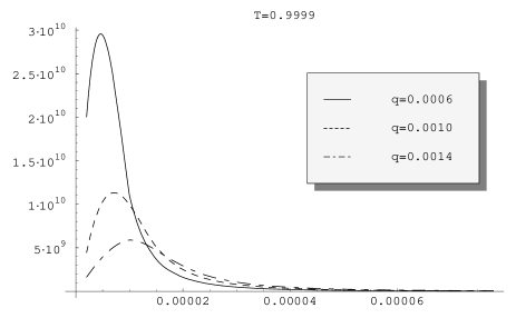
FIG. 2.: Spectral density of the NG boson at $T=0.9997$ (left) and at $T=0.9999$ (right) as a function of energy. Everything is measured in units of $T_{c}$.

In order to cross-check our analytical studies, we have also performed a numerical analysis of the NG boson spectral density. Such a density is defined by the imaginary part of the corresponding propagator. In the numerics, we have used the approximation of small energy and momenta, but we have not used any assumptions about the value of the superconducting gap. The results are plotted in Fig. 2 for two values of temperature, $T=0.9997T_{c}$ (corresponding to $|\Delta_{T}|=0.053T_{c}$) and $T=0.9999T_{c}$ (corresponding to $|\Delta_{T}|=0.031T_{c}$). As is easy to check, the energy location of the maxima scale with momenta in accordance with a linear dispersion law that is very similar to that in Eq. (135).

IX CG modes

Now, let us consider a special type of collective modes, the so-called Carlson-Goldman gapless modes. Such modes were experimentally discovered by Carlson and Goldman about a three decades ago [30] (see also, Ref. [31, 40, 41, 42, 43, 44, 45]). One of the most intriguing interpretation connects such modes with a revival of the Nambu-Goldstone (NG) bosons in the superconducting phase where the Anderson-Higgs mechanism should commonly take place. It was argued that an interplay of two effects, screening and Landau damping, is crucial for the existence of the CG modes [31]. These modes can only appear in the vicinity of the critical temperature (in the broken phase), where a large number of thermally excited quasiparticles leads to partial screening of the Coulomb interaction, and the Anderson-Higgs mechanism becomes inefficient. At the same time, the quasiparticles induce Landau damping which usually makes the CG modes overdamped in clean systems. To suppress such an effect and make the CG modes observable, one should consider dirty systems in which quasiparticle scatterings on impurities tend to reduce Landau damping.

In the two fluid description, the CG modes are related to oscillations of the superfluid and the normal component in opposite directions [40]. The local charge density remains zero in such oscillations, providing favorable conditions for gapless modes, in contrary to the widespread belief that the plasmons are the only collective modes in charged systems.

The CG modes exist only in the presence of a large number of thermally excited quasiparticles (normal component). This means, therefore, that such modes could live only in a finite (possibly very small) vicinity of the critical temperature.

In the nearcritical region, from Eq. (89) we derive the following approximate equation for the spectrum of the collective modes of electric type (assuming that $|\Delta_{T}|/T\ll 1$ and $v_{cg}\ll 1$ where $v_{cg}=|q_{0}|/|\vec{q}|$):

$$v_{cg}^{2}+i\frac{45\pi|\Delta_{T}|}{224T}v_{cg}-\frac{9\zeta(3)|\Delta_{T}|^{2}}{8\pi^{2}T^{2}}=0.$$ (136)

The derivation of this relation is similar to the derivation of Eq. (134) in the case of the NG bosons. It might look surprising, but Eq. (136) is qualitatively the same as Eq. (134). The solution to this dispersion equation reads

$$q_{0}=\frac{|\Delta_{T}|}{T}(\pm x_{cg}^{*}-iy_{cg}^{*})|\vec{q}|,$$ (137)

where $x_{cg}^{*}\approx 0.193$ and $y_{cg}^{*}\approx 0.316$. This solution corresponds to the gapless CG modes, and it closely resembles the dispersion relation of the NG bosons in Eq. (135). The width of these CG modes is quite large, but this should not be surprising because we consider the clean limit of the dense quark matter.

The numerical solution for $v_{cg}$ as a function of temperature in Fig. 3. To plot the figure, we used the standard Bardeen-Cooper-Schrieffer (BCS) dependence of the value of the gap on temperature, obtained from the following implicit expression:

$$\ln\frac{\pi T_{c}}{e^{\gamma}|\Delta_{T}|}=\int_{0}^{\infty}\frac{d\epsilon\left(1-\tanh\frac{1}{2T}\sqrt{\epsilon^{2}+|\Delta_{T}|^{2}}\right)}{\sqrt{\epsilon^{2}+|\Delta_{T}|^{2}}},$$ (138)

where $\gamma\approx 0.567$ is the Euler constant. As was shown in Ref. [14], such a dependence remains adequate in the case of a color superconductor.

 

FIG. 3.: Left: The real (solid line) and imaginary (dash line) parts of the numerical solution for $v=q_{0}/|\vec{q}|$. Right: Temperature dependence of the color superconducting gap.

It has to be emphasized that the result in Eq. (137) is obtained for a clean system where Landau damping effects have their full strength. Therefore, it should have been expected that the CG modes are overdamped. However, our analysis shows that the presence of two different types of quarks with nonequal gaps in the CFL phase plays the key role in a partial suppression of Landau damping. Indeed, as is straightforward to check, if the values of the gaps in both the octet and singlet channels were equal, the dispersion relation of the CG modes would be given by

$$v=-i\frac{14\zeta(3)|\Delta_{T}|}{3\pi^{3}T}+\ldots,$$ (139)

where the higher order terms in powers of $|\Delta_{T}|/T$ are denoted by the ellipsis. We see from this result that the ratio of the imaginary and real parts is much larger than 1 (in fact, it is infinite in this leading order approximation), meaning that the CG modes are unobservable in the case of equal gaps. In contrast to this, the CG modes with the dispersion relation in Eq. (137) could be observable (see our results for the electric gluon spectral density below).

From the numerical result, we clearly see that the ratio of the width, $\Gamma=-2Im(v_{cg})|\vec{q}|$, to the energy of the CG mode, $\varepsilon_{q}=Re(v_{cg})|\vec{q}|$, increases when the temperature of the system goes further away from the critical point. At temperature $T^{*}\approx 0.986T_{c}$, this ratio formally goes to infinity. This value of $T^{*}$ gives an estimate of temperature where the CG mode disappears. Of course, such an estimate is not very reliable since our approximations should break before the temperature $T^{*}$ is reached. In order to get a better estimate of temperature where the CG mode disappears, a more careful numerical calculation is required.

 

FIG. 4.: Spectral density of the electric gluon at $T=0.9997$ (left) and at $T=0.9999$ (right) as a function of energy. Everything is measured in units of $T_{c}$.

As in the case of the NG bosons, we have also performed a numerical analysis of the electric gluon spectral density in the region of small momenta where the trace of the CG modes is expected to appear. In our numerical calculation, we have used the approximation of small energy and momenta. The results are plotted in Fig. 4 for two values of temperature, $T=0.9997T_{c}$ (corresponding to $|\Delta_{T}|=0.053T_{c}$) and $T=0.9999T_{c}$ (corresponding to $|\Delta_{T}|=0.031T_{c}$). Although the maxima in the electron gluon spectral densities are not so well pronounced as in the case of the spectral densities of the NG bosons (see Fig. 2 in the preceding section), they are detectable when temperatures are sufficiently close to $T_{c}$. One could also check that the energy location of the maxima in Fig. 4 scale with momenta in accordance with a linear dispersion law similar to that in Eq. (137).

X Meissner effect

Now, let us discuss the Meissner effect at finite temperature. This can be done by examining the response of the quark system to an external static magnetic field. In order to derive the expression for the magnetic $\Pi_{1}(q)$ component of the polarization tensor in the limit $|q_{0}|\ll|\vec{q}|\to 0$, let us start with the calculation of the $H(q_{0}=0,|{\vec{q}}|)$ function,

$$H(|{\vec{q}}|) = -1+\frac{T}{12}\sum_{n}\int\limits_{-1}^{1}d\xi(1-\xi^{2})\int d\epsilon\left[\frac{2|\Delta_{T}|^{2}-7\epsilon^{2}+7\frac{q^{2}\xi^{2}}{4}+7\omega_{n}^{2}}{(\omega_{n}^{2}+E_{-}^{2})(\omega_{n}^{2}+E_{+}^{2})}\right.$$ (140)

$$+ \left.\frac{2|\Delta_{T}|^{2}-\epsilon^{2}+\frac{q^{2}\xi^{2}}{4}+\omega_{n}^{2}}{(\omega_{n}^{2}+E_{-}^{2})(\omega_{n}^{2}+\tilde{E}_{+}^{2})}+\frac{2|\Delta_{T}|^{2}-\epsilon^{2}+\frac{q^{2}\xi^{2}}{4}+\omega_{n}^{2}}{(\omega_{n}^{2}+\tilde{E}_{-}^{2})(\omega_{n}^{2}+E_{+}^{2})}\right],$$ (141)

where $E_{\pm}^{2}=(\epsilon\pm q\xi/2)^{2}+|\Delta_{T}|^{2}$ and $\tilde{E}_{\pm}^{2}=(\epsilon\pm q\xi/2)^{2}+4|\Delta_{T}|^{2}$. The proper calculation of this expression requires performing the Matsubara summation before integrating over $\epsilon$. This order could be interchanged if the normal phase contribution (with $\Delta_{T}=0$) is subtracted from the above expression, i.e.,

$$H(|{\vec{q}}|) = H_{0}(|{\vec{q}}|)+[H(|{\vec{q}}|)-H_{0}(|{\vec{q}}|)]=H_{0}(|{\vec{q}}|)+\frac{T}{12}\sum_{n}\int\limits_{-1}^{1}d\xi(1-\xi^{2})\int d\epsilon\left[\frac{2|\Delta_{T}|^{2}-7\epsilon^{2}+7\frac{q^{2}\xi^{2}}{4}+7\omega_{n}^{2}}{(\omega_{n}^{2}+E_{-}^{2})(\omega_{n}^{2}+E_{+}^{2})}\right.$$ (142)

$$+ \left.\frac{2|\Delta_{T}|^{2}-\epsilon^{2}+\frac{q^{2}\xi^{2}}{4}+\omega_{n}^{2}}{(\omega_{n}^{2}+E_{-}^{2})(\omega_{n}^{2}+\tilde{E}_{+}^{2})}+\frac{2|\Delta_{T}|^{2}-\epsilon^{2}+\frac{q^{2}\xi^{2}}{4}+\omega_{n}^{2}}{(\omega_{n}^{2}+\tilde{E}_{-}^{2})(\omega_{n}^{2}+E_{+}^{2})}-9\frac{-\epsilon^{2}+\frac{q^{2}\xi^{2}}{4}+\omega_{n}^{2}}{(\omega_{n}^{2}+(\epsilon-q\xi/2)^{2})(\omega_{n}^{2}+(\epsilon+q\xi/2)^{2})}\right].$$ (143)

It is easy to check that performing summation over Matsubara frequencies (and taking the limit $|{\vec{q}}|\to 0$) we come back to Eq. (92) (where we put first $q_{0}=0$ first and then $|{\vec{q}}|=0$). Notice that the last term in square brackets in Eq. (143) reproduces the first term on the right hand side in Eq. (92).

The nice feature about Eq. (143) is that it allows to interchange the order of summation and integration. This is because the integral and the sum converge rapidly. The initial expression for $H(q_{0},|\vec{q}|)$ did not have this property, and the order of operations was fixed (first summation, then integration). By evaluating the integral over $\epsilon$ in Eq. (143), we obtain

$$H(|{\vec{q}}|) = \frac{\pi T|\Delta_{T}|^{2}}{12}\sum_{n}\int\limits_{-1}^{1}d\xi(1-\xi^{2})\left\{-\frac{5/2}{\sqrt{\omega_{n}^{2}+|\Delta_{T}|^{2}}(\omega_{n}^{2}+|\Delta_{T}|^{2}+q^{2}\xi^{2}/4)}\right.$$ (144)

$$+ \left.\frac{6}{9|\Delta_{T}|^{4}+2q^{2}\xi^{2}(2\omega_{n}^{2}+5|\Delta_{T}|^{2}+q^{2}\xi^{2}/2)}\left[\frac{2\omega_{n}^{2}+3|\Delta_{T}|^{2}+q^{2}\xi^{2}/3}{\sqrt{\omega_{n}^{2}+|\Delta_{T}|^{2}}}-\frac{2(\omega_{n}^{2}+3|\Delta_{T}|^{2}+q^{2}\xi^{2}/3)}{\sqrt{\omega_{n}^{2}+4|\Delta_{T}|^{2}}}\right]\right\}.$$ (145)

From the structure of this expression, it is clear that $|{\vec{q}}|/T_{c}$ is an important dimensionless parameter at all temperatures. Indeed, for $T\ll T_{c}$, it is the gap $|\Delta_{0}|$ which of order $T_{c}$ that sets the scale in the $H(|{\vec{q}}|)$ function. Near $T_{c}$ (i.e., $|T_{c}-T|\ll T_{c}$), on the other hand, the gap is small but $\omega_{n\neq 0}=2n\pi T\simeq T_{c}$ gives the same characteristic scale.

Let us begin by examining the first limiting case, $|{\vec{q}}|\ll T_{c}$. In this limit, we keep only the leading order term on the right hand side of Eq. (145), and drop all terms suppressed by a power of $|{\vec{q}}|$. Thus, we arrive at

$$H(|{\vec{q}}|)\simeq\frac{\pi T|\Delta_{T}|^{2}}{9}\sum_{n}\left\{\frac{-5/2}{(\omega_{n}^{2}+|\Delta_{T}|^{2})^{3/2}}+\frac{4}{3|\Delta_{T}|^{4}}\left(\frac{\omega_{n}^{2}+3|\Delta_{T}|^{2}/2}{\sqrt{\omega_{n}^{2}+|\Delta_{T}|^{2}}}-\frac{\omega_{n}^{2}+3|\Delta_{T}|^{2}}{\sqrt{\omega_{n}^{2}+4|\Delta_{T}|^{2}}}\right)\right\}.$$ (146)

As a benchmark test, let us calculate this expression at $T=0$. The sum over frequencies in this case can be replaced by an integral, by setting $2\pi T\delta n=d\omega$. Thus, we arrive at the result

$$H(|\vec{q}|\to 0) = \frac{|\Delta_{T}|^{2}}{18}\int\limits_{-\infty}^{\infty}d\omega\left[\frac{-5/2}{(\omega^{2}+|\Delta_{T}|^{2})^{3/2}}+\frac{4}{3|\Delta_{T}|^{4}}\left(\frac{\omega^{2}+3|\Delta_{T}|^{2}/2}{\sqrt{\omega^{2}+|\Delta_{T}|^{2}}}-\frac{\omega^{2}+3|\Delta_{T}|^{2}}{\sqrt{\omega^{2}+4|\Delta_{T}|^{2}}}\right)\right]$$ (147)

$$= \frac{1}{9}\int\limits_{0}^{\infty}dx\left[\frac{-5/2}{(x^{2}+1)^{3/2}}+\frac{4}{3}\left(\frac{x^{2}+3/2}{\sqrt{x^{2}+1}}-\frac{x^{2}+3}{\sqrt{x^{2}+4}}\right)\right]=-\frac{21-8\log{2}}{54},$$ (148)

which coincides with the known expression at zero temperature [22, 24, 26, 34].

Near the critical temperature $T_{c}$, we expand Eq. (146) in powers of $|\Delta_{T}|$ to obtain

$$H(|\vec{q}|\to 0)=-\frac{2\pi T|\Delta_{T}|^{2}}{3}\sum_{n=0}^{\infty}\frac{1}{\omega_{n}^{3}}=-\frac{7\zeta(3)|\Delta_{T}|^{2}}{12\pi^{2}T^{2}}.$$ (149)

The nonzero value of $H(|\vec{q}|\to 0)$ function in the static limit indicates that a constant magnetic field is expelled from the bulk of a superconductor. So, the conventional Meissner effect takes places at all temperatures $T<T_{c}$ in the color superconducting phase.

For completeness of our presentation, let us also determine the penetration depth of the magnetic field. To this end, we also need to calculate the behavior of the $H(|\vec{q}|)$ function for large values of $|\vec{q}|$. Thus, let us consider the limit $|{\vec{q}}|\gg T_{c}$. In this case, the main contribution to the integral over $\xi$ in Eq. (145) comes from the region $\xi\lesssim T_{c}/|{\vec{q}}|\ll 1$. In view of this observation, it is justified to neglect $-\xi^{2}$ term in the overall factor $(1-\xi^{2})$. Then, by substituting $|{\vec{q}}|\xi=x$ and expanding the limits of integration to infinity, we obtain the following approximate result:

$$H(|{\vec{q}}|) = \frac{\pi^{2}T|\Delta_{T}|^{2}}{3|{\vec{q}}|}\sum_{n\geq 0}\left[-\frac{5/2}{\omega_{n}^{2}+|\Delta_{T}|^{2}}+\frac{1}{\sqrt{\omega_{n}^{2}+|\Delta_{T}|^{2}}\sqrt{\omega_{n}^{2}+4|\Delta_{T}|^{2}}}\right.$$ (151)

$$-\left.\frac{3}{\sqrt{\omega_{n}^{2}+4|\Delta_{T}|^{2}}\left(\sqrt{\omega_{n}^{2}+4|\Delta_{T}|^{2}}+\sqrt{\omega_{n}^{2}+|\Delta_{T}|^{2}}\right)}\right],$$

or, written in slightly different form,

$$H(|{\vec{q}}|) = \frac{\pi^{2}|\Delta_{T}|^{2}}{6|{\vec{q}}|}\left[-\frac{5}{4|\Delta_{T}|}\tanh\frac{|\Delta_{T}|}{2T}+T\sum_{n\geq 0}\frac{1}{\sqrt{\omega_{n}^{2}+|\Delta_{T}|^{2}}\sqrt{\omega_{n}^{2}+4|\Delta_{T}|^{2}}}\right.$$ (153)

$$\times\left.\left(-1+\frac{9|\Delta_{T}|^{2}}{\left(\sqrt{\omega_{n}^{2}+4|\Delta_{T}|^{2}}+\sqrt{\omega_{n}^{2}+|\Delta_{T}|^{2}}\right)^{2}}\right)\right].$$

Here we explicitly performed the summation in first term and slightly rearranged the second term. In calculation leading to Eq. (151), we used the following table integrals:

$$\int\limits_{-\infty}^{\infty}\frac{dx}{x^{4}+2\beta x^{2}+1}=\int\limits_{-\infty}^{\infty}\frac{dxx^{2}}{x^{4}+2\beta x^{2}+1}=\frac{\pi}{\sqrt{2}}\frac{1}{\sqrt{\beta+1}}.$$ (154)

At zero temperature the expression (153) reduces to

$$H(|{\vec{q}}|) = \frac{\pi|\Delta_{T}|}{6|{\vec{q}}|}\left[-\frac{5\pi}{4}+\int\limits_{0}^{\infty}\frac{dx(2+x^{2}-\sqrt{x^{2}+4}\sqrt{x^{2}+1})}{\sqrt{x^{2}+4}\sqrt{x^{2}+1}}\right]$$ (155)

$$= -\frac{\pi|\Delta_{T}|}{6|{\vec{q}}|}\left[\frac{5\pi}{4}+2E\left(\frac{\sqrt{3}}{2}\right)-K\left(\frac{\sqrt{3}}{2}\right)\right].$$ (156)

Near $T_{c}$, we expand the expression in Eq. (153) in powers of $|\Delta_{T}|$, and obtain

$$H(|{\vec{q}}|)=-\frac{\pi^{2}|\Delta_{T}|^{2}}{8|{\vec{q}}|T}.$$ (157)

Now, we consider the calculation of the magnetic penetration length. By making use of the standard definition (see, for example, Ref. [46]), we obtain the following estimate:

$$\delta=\frac{1}{\pi}\int\limits_{-\infty}^{\infty}\frac{dq}{q^{2}-\omega_{p}^{2}H(q)}=\frac{2}{\pi}\left[\int\limits_{0}^{1/\xi_{0}}\frac{dq}{q^{2}+m_{M}^{2}}+\int\limits_{1/\xi_{0}}^{\infty}\frac{dq}{q^{2}+M^{2}|\Delta_{T}|/q}\right],$$ (158)

where we split the range of integration into two qualitatively different regions with momenta smaller and larger than the coherence length $\xi_{0}\sim 1/T_{c}$, respectively. The parameters $m_{M}^{2}$ and $M^{2}$ are defined as follows:

$$m_{M}^{2} = \left\{\begin{array}[]{lcc}\omega_{p}^{2}\frac{21-8\log 2}{54},&\mbox{for}&T\ll T_{c},\\ \frac{7\zeta(3)|\Delta_{T}|^{2}}{12\pi^{2}T^{2}}\omega_{p}^{2},&\mbox{for}&T\sim T_{c},\end{array}\right.$$ (161)

$$M^{2} = \left\{\begin{array}[]{lcc}M_{0}^{2}\equiv\frac{\pi}{6}\left(\frac{5\pi}{4}+2E(\sqrt{3}/2)-K(\sqrt{3}/2)\right)\omega_{p}^{2},&\mbox{for}&T\ll T_{c},\\ \frac{\pi|\Delta_{T}|}{8T}\omega_{p}^{2},&\mbox{for}&T\sim T_{c}.\end{array}\right.$$ (164)

After performing the integration in Eq. (158), we derive

$$\delta = \left\{\begin{array}[]{lcc}m_{M}^{-1}+\frac{4}{3\sqrt{3}}(M^{2}|\Delta_{T}|)^{-1/3},&\mbox{for}&(M^{2}|\Delta_{T}|)^{1/3}\gg 1/\xi_{0},\\ m_{M}^{-1},&\mbox{for}&(M^{2}|\Delta_{T}|)^{1/3}\ll 1/\xi_{0}.\end{array}\right.$$ (167)

At low temperatures, $T\ll T_{c}$, we have $1/\xi_{0}\sim|\Delta_{T}|$ and $m_{M}^{-1}\sim M_{0}^{-1}=\delta_{L}$ where $\delta_{L}$ is the London penetration depth. By taking into account that $M_{0}\simeq\omega_{p}\gg|\Delta_{T}|$, we arrive at the following low temperature expression for the penetration depth of a magnetic field:

$$\delta \equiv \delta_{P}=\frac{4}{3\sqrt{3}}(M_{0}^{2}|\Delta_{T}|)^{-1/3},\quad T\ll T_{c}.$$ (168)

This is the so-called Pippard expression for the penetration depth (note that $\delta_{P}\ll\xi_{0}$). It is easy to check from the general expression in Eq. (167) that $\delta=\delta_{P}$ almost in the whole region of temperatures $T<T_{c}$. It is also straightforward to check that the London limit (by definition, $\delta=\delta_{L}\gg\xi_{0}$) is realized only in a very close vicinity of the critical line where $|T_{c}-T|\ll T_{c}$.

XI Conclusions

In this paper, we studied collective modes coupled to (vector and axial) color current in the color-flavor locked phase of cold dense QCD at zero and finite temperatures. In this class of collective modes, we revealed and studied the ordinary plasmons, the new type of “light” plasmons, the NG bosons and, finally, the gapless CG modes.

As we argued in the main text, the properties of the ordinary (high frequency) plasmon collective excitations are similar to those in ordinary metals. The plasma frequency $\omega_{p}$ is proportional to the value of the chemical potential, and it is essentially independent of the values of the temperature and/or the superconducting gap in the dense quark matter. The “light” plasmon, on the other hand, has very different properties. It is also a massive excitation (that is why we also call it a plasmon), but the value of its mass $m_{\Delta}$ is of the order of the superconducting gap (more precisely, $1.362|\Delta_{T}|<m_{\Delta}<2|\Delta_{T}|$) which is quite small compared to $\omega_{p}$. The appearance of such a mode seems to be directly related to the existence of two different gaps in the quasiparticle spectra (in the octet and singlet channels).

In the long wave length limit $|\vec{q}|\to 0$, the “light” plasmons are stable with respect to the decays into the quark type quasiparticles. It is only because of other possible decay channels (for example, involving NG bosons), that their width might be nonzero. Now, while we have not studied the detailed dispersion relation of the “light” plasmon modes in the short wave length limit $|\vec{q}|\gtrsim|\Delta_{T}|$, it is expected that their energy is a monotonically increasing function of momentum $|\vec{q}|$. If this is true, there should exist a critical value of the wave length of order $1/|\Delta_{T}|$ at which the energy of the “light” plasmon becomes equal to the threshold of the quasiparticle pair production. The excitations with the wave lengths shorter than the critical value (and the energy larger than $2|\Delta_{T}|$) could easily decay into quasiparticles and, therefore, should have a relatively large width. It means that these new type plasmon modes have two characteristic plasma frequencies, $m_{\Delta}$ and $2|\Delta_{T}|$. The stable (narrow width) modes live only in the following window of the energies, $m_{\Delta}<q_{0}<2|\Delta_{T}|$.

The properties of the NG bosons in the CFL phase at zero temperature are well studied in the literature. Here we generalized such studies to the case of finite temperatures. In particular, we showed that the NG boson properties at small temperatures remain almost the same as at zero temperature, having an exponentially small width. With increasing the temperature, the width also increases. We presented analytical study of the dispersion relation of NG bosons in the nearcritical region of temperatures. Our result confirms the general expectation of the slowdown of the NG bosons in this region, where their maximum velocity is proportional to the small value of the color superconducting gap.

By making use of an explicitly gauge covariant approach, we also studied the properties of the gapless CG modes in the CFL phase of cold dense quark matter in the nearcritical region (just below $T_{c}$) where a considerable density of thermally excited quasiparticles is present. It is important to mention that the presence of the CG modes coexists with the usual Meissner effect, i.e., an external static magnetic field is expelled from the bulk of a superconductor. The existence of the Meissner effect is a clear signature that the system remains in the symmetry broken (superconducting) phase.

In the case of the CFL phase, as we showed, the CG modes appear even in the clean limit. Despite the sizable width, their traces can be observed in the spectral density of the electric gluons. Taking the effect of impurities into account should, in general, make the CG modes more pronounced [44]. In realistic systems such as compact stars, natural impurities of different nature could further improve the quality of the gapless CG modes.

The existence of a gapless scalar CG modes (in addition to the pseudoscalar NG bosons) is a very important property of the color superconducting phase. They may affect thermodynamical as well as transport properties of the system in the nearcritical region. In its turn, this might have a profound effect on the evolution of forming compact stars. The CG modes might also have a consequence on a possible existence of the hypothetical quark-hadron continuity, suggested in Ref. [47]. Indeed, one should notice that, in the hadron phase, there does not seem to exist any low energy excitations with the quantum numbers matching those of the CG modes.

In the future, it would be interesting to generalize our analysis to the so-called $S2C$ phase of dense QCD. In absence of true NG bosons in the $S2C$ phase, the gapless CG modes might play a more important role. Our general observations suggest that Landau damping should have stronger influence in the case of two flavors. At the same time, the presence of massless quarks could lead to widening the range of temperatures where the CG modes exist. To make a more specific prediction, one should study the problem in detail.

A Identities, formulas, etc.

In the main text we use the following identities for the structure constants of $SU(3)$:

$$d^{ACD}d^{BCD}=\frac{5}{3}\delta^{AB},$$ (A1)

$$f^{ACD}f^{BCD}=3\delta^{AB}.$$ (A2)

For completeness, we also present the following more complicated identities:

$$d^{AA^{\prime}B^{\prime}}d^{BB^{\prime}C^{\prime}}d^{CC^{\prime}A^{\prime}} = -\frac{1}{2}d^{ABC},$$ (A3)

$$d^{AA^{\prime}B^{\prime}}d^{BB^{\prime}C^{\prime}}f^{CC^{\prime}A^{\prime}} = -\frac{5}{6}f^{ABC},$$ (A4)

$$d^{AA^{\prime}B^{\prime}}f^{BB^{\prime}C^{\prime}}f^{CC^{\prime}A^{\prime}} = -\frac{3}{2}d^{ABC},$$ (A5)

$$f^{AA^{\prime}B^{\prime}}f^{BB^{\prime}C^{\prime}}f^{CC^{\prime}A^{\prime}} = \frac{3}{2}f^{ABC}.$$ (A6)

In this Appendix, we also derive the three types of Matsubara summation formulas that appear in the main text. By convention, we use the notation $\omega_{n}=T\pi(2n+1)$, $\Omega_{m}=2T\pi m$ and $\beta=1/T$. The mentioned three types of sums are

$$F_{1}(i\Omega_{m};a,b) = T\sum_{n}\frac{1}{\left(\omega_{n}^{2}+a^{2}\right)\left[(\omega_{n}+\Omega_{m})^{2}+b^{2}\right]},$$ (A7)

$$F_{2}(i\Omega_{m};a,b) = T\sum_{n}\frac{i\omega_{n}}{\left(\omega_{n}^{2}+a^{2}\right)\left[(\omega_{n}+\Omega_{m})^{2}+b^{2}\right]},$$ (A8)

$$F_{3}(i\Omega_{m};a,b) = T\sum_{n}\frac{\omega_{n}(\omega_{n}+\Omega_{m})}{\left(\omega_{n}^{2}+a^{2}\right)\left[(\omega_{n}+\Omega_{m})^{2}+b^{2}\right]}.$$ (A9)

Let us start from the first one. The sum is performed by going to the complex plane and introducing the contour integral. The result is

$$F_{1}(i\Omega_{m};a,b) = \frac{b(\Omega_{m}^{2}-a^{2}+b^{2})\tanh(a\beta/2)+a(\Omega_{m}^{2}+a^{2}-b^{2})\tanh(b\beta/2)}{2ab\left[(a+b)^{2}+\Omega_{m}^{2}\right]\left[(a-b)^{2}+\Omega_{m}^{2}\right]}$$ (A10)

$$= \frac{(a+b)\left[1-n(a)-n(b)\right]}{2ab\left[(a+b)^{2}+\Omega_{m}^{2}\right]}+\frac{(a-b)\left[n(a)-n(b)\right]}{2ab\left[(a-b)^{2}+\Omega_{m}^{2}\right]},$$ (A11)

where

$$n(a)=\frac{1}{\exp(a\beta)+1}$$ (A12)

is the Fermi distribution function.

To perform the analytical continuation to the real frequencies, we substitute $i\Omega_{m}=\Omega+i\eta$ where $\eta$ is a vanishingly small positive constant. In this way, we arrive at

$$F_{1}(\Omega;a,b) = -{\cal P.V.}\frac{(a+b)\left[1-n(a)-n(b)\right]}{2ab\left[\Omega^{2}-(a+b)^{2}\right]}-{\cal P.V.}\frac{(a-b)\left[n(a)-n(b)\right]}{2ab\left[\Omega^{2}-(a-b)^{2}\right]}$$ (A15)

$$+i\frac{\pi(a+b)}{2ab}\mbox{sgn}(\Omega)\delta\left(\Omega^{2}-(a+b)^{2}\right)\left[1-n(a)-n(b)\right]$$

$$+i\frac{\pi(a-b)}{2ab}\mbox{sgn}(\Omega)\delta\left(\Omega^{2}-(a-b)^{2}\right)\left[n(a)-n(b)\right].$$

Similarly,

$$F_{2}(i\Omega_{m};a,b) = \frac{i\Omega_{m}\left[2ab\tanh(a\beta/2)-(a^{2}+b^{2}+\Omega_{m}^{2})\tanh(b\beta/2)\right]}{2b\left[(a+b)^{2}+\Omega_{m}^{2}\right]\left[(a-b)^{2}+\Omega_{m}^{2}\right]}$$ (A16)

$$= -\frac{i\Omega_{m}\left[1-n(a)-n(b)\right]}{2b\left[(a+b)^{2}+\Omega_{m}^{2}\right]}-\frac{i\Omega_{m}\left[n(a)-n(b)\right]}{2b\left[(a-b)^{2}+\Omega_{m}^{2}\right]},$$ (A17)

$$F_{3}(i\Omega_{m};a,b) = \frac{a(a^{2}-b^{2}+\Omega_{m}^{2})\tanh(a\beta/2)+b(b^{2}-a^{2}+\Omega_{m}^{2})\tanh(b\beta/2)}{2\left[(a+b)^{2}+\Omega_{m}^{2}\right]\left[(a-b)^{2}+\Omega_{m}^{2}\right]}$$ (A18)

$$= \frac{(a+b)\left[1-n(a)-n(b)\right]}{2\left[(a+b)^{2}+\Omega_{m}^{2}\right]}-\frac{(a-b)\left[n(a)-n(b)\right]}{2\left[(a-b)^{2}+\Omega_{m}^{2}\right]},$$ (A19)

and

$$F_{2}(\Omega;a,b) = {\cal P.V.}\frac{\Omega\left[1-n(a)-n(b)\right]}{2b\left[\Omega^{2}-(a+b)^{2}\right]}+{\cal P.V.}\frac{\Omega\left[n(a)-n(b)\right]}{2b\left[\Omega^{2}-(a-b)^{2}\right]}$$ (A22)

$$-i\frac{\pi|\Omega|}{2b}\delta\left(\Omega^{2}-(a+b)^{2}\right)\left[1-n(a)-n(b)\right]$$

$$-i\frac{\pi|\Omega|}{2b}\delta\left(\Omega^{2}-(a-b)^{2}\right)\left[n(a)-n(b)\right]$$

$$F_{3}(\Omega;a,b) = -{\cal P.V.}\frac{(a+b)\left[1-n(a)-n(b)\right]}{2\left[\Omega^{2}-(a+b)^{2}\right]}+{\cal P.V.}\frac{(a-b)\left[n(a)-n(b)\right]}{2\left[\Omega^{2}-(a-b)^{2}\right]}$$ (A25)

$$+i\frac{\pi(a+b)}{2}\mbox{sgn}(\Omega)\delta\left(\Omega^{2}-(a+b)^{2}\right)\left[1-n(a)-n(b)\right]$$

$$-i\frac{\pi(a-b)}{2}\mbox{sgn}(\Omega)\delta\left(\Omega^{2}-(a-b)^{2}\right)\left[n(a)-n(b)\right].$$

The typical expressions for $a$ and $b$ would be given by

$$a = \sqrt{\Delta_{1}^{2}+(\epsilon-\xi|\vec{q}|/2)^{2}},$$ (A26)

$$b = \sqrt{\Delta_{2}^{2}+(\epsilon+\xi|\vec{q}|/2)^{2}},$$ (A27)

where $\epsilon=|\vec{p}|-\mu$, $\xi=\cos\theta$ and $\theta$ is the angle between the spatial vectors $\vec{p}$ and $\vec{q}$.

The $\delta$-functions that appear in the imaginary terms of all three sums have the singularities at

$$\epsilon^{\pm}_{0} = \frac{|\vec{q}|\xi(\Delta_{2}^{2}-\Delta_{1}^{2})\pm\Omega\sqrt{[\Omega^{2}-|\vec{q}|^{2}\xi^{2}-(\Delta_{1}-\Delta_{2})^{2}][\Omega^{2}-|\vec{q}|^{2}\xi^{2}-(\Delta_{1}+\Delta_{2})^{2}]}}{2(\Omega^{2}-|\vec{q}|^{2}\xi^{2})},$$ (A28)

which is real only when $\Omega^{2}\leq(\Delta_{1}-\Delta_{2})^{2}+|\vec{q}|^{2}\xi^{2}$, or when $\Omega^{2}\geq(\Delta_{1}+\Delta_{2})^{2}+|\vec{q}|^{2}\xi^{2}$. The first region defines the window of energies in which the Landau damping operates, while the other region corresponds to energies for which the on-shell pair production of quasiparticles is allowed.

B Operators $O^{(i)}$

In the main text of the paper, we heavily use the following set of four tensors:

$$O^{(1)}_{\mu\nu}(q) = g_{\mu\nu}-u_{\mu}u_{\nu}+\frac{\vec{q}_{\mu}\vec{q}_{\nu}}{|\vec{q}|^{2}},$$ (B1)

$$O^{(2)}_{\mu\nu}(q) = u_{\mu}u_{\nu}-\frac{\vec{q}_{\mu}\vec{q}_{\nu}}{|\vec{q}|^{2}}-\frac{q_{\mu}q_{\nu}}{q^{2}},$$ (B2)

$$O^{(3)}_{\mu\nu}(q) = \frac{q_{\mu}q_{\nu}}{q^{2}},$$ (B3)

$$O^{(4)}_{\mu\nu}(q) = O^{(2)}_{\mu\lambda}u^{\lambda}\frac{q_{\nu}}{|\vec{q}|}+\frac{q_{\mu}}{|\vec{q}|}u^{\lambda}O^{(2)}_{\lambda\nu}.$$ (B4)

The first three of them are the same projectors of the magnetic, electric and unphysical (longitudinal in a 3+1 dimensional sense) modes of gluons which were used in Ref. [7]. In addition, here we also introduced the intervening operator $O^{(4)}_{\mu\nu}(q)$, mixing the electric and unphysical modes. In the above definitions of $O^{(i)}_{\mu\nu}(q)$, we use

$$u_{\mu} = (1,0,0,0),$$ (B5)

$$\vec{q}_{\mu} = q_{\mu}-(u\cdot q)u_{\mu}.$$ (B6)

By making use of the explicit form of the operators $O^{(i)}$, it is straightforward to derive the following relations:

$$u_{\mu}u_{\nu} = -\frac{|\vec{q}|^{2}}{q^{2}}O^{(2)}_{\mu\nu}(q)+\frac{q_{0}^{2}}{q^{2}}O^{(3)}_{\mu\nu}(q)+\frac{q_{0}|\vec{q}|}{q^{2}}O^{(4)}_{\mu\nu}(q),$$ (B7)

$$\frac{u_{\mu}\vec{q}_{\nu}+\vec{q}_{\mu}u_{\nu}}{|\vec{q}|} = \frac{2q_{0}|\vec{q}|}{q^{2}}\left[O^{(2)}_{\mu\nu}(q)-O^{(3)}_{\mu\nu}(q)\right]-\frac{q_{0}^{2}+|\vec{q}|^{2}}{q^{2}}O^{(4)}_{\mu\nu}(q),$$ (B8)

as well as the following multiplication rules:

$$O^{(1)}(q)O^{(1)}(q) = O^{(1)}(q),$$ (B9)

$$O^{(2)}(q)O^{(2)}(q) = O^{(2)}(q),$$ (B10)

$$O^{(3)}(q)O^{(3)}(q) = O^{(3)}(q),$$ (B11)

$$O^{(1)}(q)O^{(2)}(q) = O^{(2)}(q)O^{(1)}(q)=0,$$ (B12)

$$O^{(1)}(q)O^{(3)}(q) = O^{(3)}(q)O^{(1)}(q)=0,$$ (B13)

$$O^{(2)}(q)O^{(3)}(q) = O^{(3)}(q)O^{(2)}(q)=0,$$ (B14)

$$O^{(4)}(q)O^{(4)}(q) = -O^{(2)}(q)-O^{(3)}(q),$$ (B15)

$$O^{(4)}(q)O^{(1)}(q) = O^{(1)}(q)O^{(4)}(q)=0,$$ (B16)

$$O^{(4)}(q)O^{(2)}(q) = O^{(3)}(q)O^{(4)}(q),$$ (B17)

$$O^{(4)}(q)O^{(3)}(q) = O^{(2)}(q)O^{(4)}(q).$$ (B18)

In these last expressions, proper contractions of the Lorentz indices are tacitly assumed.

The structure of the polarization tensor as well as the structure of the gluon propagator in the main text are given in terms of the $O^{(i)}$ operators. It is very useful, therefore, to know how to invert the corresponding tensors. By making use of the definitions in Eqs. (B1) – (B4), we check that the following statement is true. If a general matrix (in Lorentz indices) allows the following decomposition in terms of the operators $O^{(i)}$

$$A=aO^{(1)}(q)+bO^{(2)}(q)+cO^{(3)}(q)+dO^{(4)}(q),$$ (B19)

its inverse matrix is given by

$$A^{-1}=\frac{1}{a}O^{(1)}(q)+\frac{c}{bc+d^{2}}O^{(2)}(q)+\frac{b}{bc+d^{2}}O^{(3)}(q)-\frac{d}{bc+d^{2}}O^{(4)}(q).$$ (B20)

C Calculation of $\Pi_{\mu\nu}$

In the Appendix, we calculate the expression of $\Pi_{\mu\nu}$ in different limits. The complete expression for the polarization tensor contains a sum of the left- and right-handed contributions [only one of them is given in Eq. (31) in the main text]:

$$\Pi_{\mu\nu}^{AB}(q)=\Pi_{L,\mu\nu}^{AB}(q)+\Pi_{R,\mu\nu}^{AB}(q)\equiv\delta^{AB}\Pi_{\mu\nu}(q).$$ (C1)

The complete one-loop result (in Minkowski space) is given by

$$\Pi_{\mu\nu}(\Omega,q) = \frac{g^{2}}{12}\sum_{e,e^{\prime}=\pm}\int\frac{d^{3}p}{(2\pi)^{3}}$$ (C2)

$$\times \Bigg{\{}ee^{\prime}\epsilon^{e}_{p-q/2}\epsilon^{e^{\prime}}_{p+q/2}T^{e,e^{\prime}}_{\mu\nu}\left[7F_{1}(\Omega;E^{e}_{p-q/2},E^{e^{\prime}}_{p+q/2})+F_{1}(\Omega;E^{e}_{p-q/2},\tilde{E}^{e^{\prime}}_{p+q/2})+F_{1}(\Omega;\tilde{E}^{e}_{p-q/2},E^{e^{\prime}}_{p+q/2})\right]$$ (C7)

$$-T^{e,e^{\prime}}_{\mu\nu}\left[7F_{3}(\Omega;E^{e}_{p-q/2},E^{e^{\prime}}_{p+q/2})+F_{3}(\Omega;E^{e}_{p-q/2},\tilde{E}^{e^{\prime}}_{p+q/2})+F_{3}(\Omega;\tilde{E}^{e}_{p-q/2},E^{e^{\prime}}_{p+q/2})\right]$$

$$+(e\epsilon^{e}_{p-q/2}+e^{\prime}\epsilon^{e^{\prime}}_{p+q/2})U^{e,e^{\prime}}_{\mu\nu}\left[7F_{2}(\Omega;E^{e}_{p-q/2},E^{e^{\prime}}_{p+q/2})+F_{2}(\Omega;E^{e}_{p-q/2},\tilde{E}^{e^{\prime}}_{p+q/2})+F_{2}(\Omega;\tilde{E}^{e}_{p-q/2},E^{e^{\prime}}_{p+q/2})\right]$$

$$+\Omega e\epsilon^{e}_{p-q/2}U^{e,e^{\prime}}_{\mu\nu}\left[7F_{1}(\Omega;E^{e}_{p-q/2},E^{e^{\prime}}_{p+q/2})+F_{1}(\Omega;E^{e}_{p-q/2},\tilde{E}^{e^{\prime}}_{p+q/2})+F_{1}(\Omega;\tilde{E}^{e}_{p-q/2},E^{e^{\prime}}_{p+q/2})\right]$$

$$+2|\Delta_{T}|^{2}V^{e,e^{\prime}}_{\mu\nu}\left[F_{1}(\Omega;E^{e}_{p-q/2},E^{e^{\prime}}_{p+q/2})+F_{1}(\Omega;E^{e}_{p-q/2},\tilde{E}^{e^{\prime}}_{p+q/2})+F_{1}(\Omega;\tilde{E}^{e}_{p-q/2},E^{e^{\prime}}_{p+q/2})\right]\Bigg{\}},$$

where the tensor structures are

$$T^{e,e^{\prime}}_{\mu\nu} = \mbox{tr}\left(\gamma_{\mu}\gamma_{0}\Lambda^{-e}_{p-q/2}\gamma_{\nu}\gamma_{0}\Lambda^{-e^{\prime}}_{p+q/2}\right)+\mbox{tr}\left(\gamma_{\mu}\gamma_{0}\Lambda^{e}_{p-q/2}\gamma_{\nu}\gamma_{0}\Lambda^{e^{\prime}}_{p+q/2}\right),$$ (C8)

$$U^{e,e^{\prime}}_{\mu\nu} = \mbox{tr}\left(\gamma_{\mu}\gamma_{0}\Lambda^{-e}_{p-q/2}\gamma_{\nu}\gamma_{0}\Lambda^{-e^{\prime}}_{p+q/2}\right)-\mbox{tr}\left(\gamma_{\mu}\gamma_{0}\Lambda^{e}_{p-q/2}\gamma_{\nu}\gamma_{0}\Lambda^{e^{\prime}}_{p+q/2}\right),$$ (C9)

$$V^{e,e^{\prime}}_{\mu\nu} = \mbox{tr}\left(\gamma_{\mu}\Lambda^{-e}_{p-q/2}\gamma_{\nu}\Lambda^{e^{\prime}}_{p+q/2}\right)+\mbox{tr}\left(\gamma_{\mu}\Lambda^{e}_{p-q/2}\gamma_{\nu}\Lambda^{-e^{\prime}}_{p+q/2}\right),$$ (C10)

and

$$E^{e}_{k} = \sqrt{(\epsilon^{e}_{k})^{2}+|\Delta_{T}|^{2}},$$ (C11)

$$\tilde{E}^{e}_{k} = \sqrt{(\epsilon^{e}_{k})^{2}+4|\Delta_{T}|^{2}},$$ (C12)

are the excitation energies in the octet and the singlet channels, respectively.

The general expression in Eq. (C7) can be approximated by dropping all the subleading terms. For large chemical potential, we derive the following approximate expression:

$$\Pi_{\mu\nu}(\Omega,q) = \frac{g^{2}\mu^{2}}{2\pi^{2}}\left(u_{\mu}u_{\nu}-g_{\mu\nu}\right)$$ (C14)

$$+\frac{g^{2}\mu^{2}}{12\pi^{2}}\int_{-1}^{1}d\xi\int d\epsilon\Bigg{\{}2|\Delta_{T}|^{2}\left(u_{\mu}u_{\nu}(1-\xi^{2})+\xi^{2}g_{\mu\nu}+\frac{1-3\xi^{2}}{2}O^{(1)}_{\mu\nu}(q)\right)$$

$$\times \left[F_{1}(\Omega;E_{-},E_{+})+F_{1}(\Omega;E_{-},\tilde{E}_{+})+F_{1}(\Omega;\tilde{E}_{-},E_{+})\right]$$ (C15)

$$+ \left(\epsilon^{2}-\xi^{2}|\vec{q}|^{2}/4\right)\left(u_{\mu}u_{\nu}(1+\xi^{2})-\xi^{2}g_{\mu\nu}-\frac{1-3\xi^{2}}{2}O^{(1)}_{\mu\nu}(q)\right)$$ (C16)

$$\times \left[7F_{1}(\Omega;E_{-},E_{+})+F_{1}(\Omega;E_{-},\tilde{E}_{+})+F_{1}(\Omega;\tilde{E}_{-},E_{+})\right]$$ (C17)

$$- \frac{1}{2}\xi^{2}\Omega(u_{\nu}\vec{q}_{\mu}+u_{\mu}\vec{q}_{\nu})\left[7F_{1}(\Omega;E_{-},E_{+})+F_{1}(\Omega;E_{-},\tilde{E}_{+})+F_{1}(\Omega;\tilde{E}_{-},E_{+})\right]$$ (C18)

$$- \left(u_{\mu}u_{\nu}(1+\xi^{2})-\xi^{2}g_{\mu\nu}-\frac{1-3\xi^{2}}{2}O^{(1)}_{\mu\nu}(q)\right)$$ (C19)

$$\times \left[7F_{3}(\Omega;E_{-},E_{+})+F_{3}(\Omega;E_{-},\tilde{E}_{+})+F_{3}(\Omega;\tilde{E}_{-},E_{+})\right]$$ (C20)

$$+ 2\epsilon\xi\frac{u_{\nu}\vec{q}_{\mu}+u_{\mu}\vec{q}_{\nu}}{|\vec{q}|}\left[7F_{2}(\Omega;E_{-},E_{+})+F_{2}(\Omega;E_{-},\tilde{E}_{+})+F_{2}(\Omega;\tilde{E}_{-},E_{+})\right]\Bigg{\}}.$$ (C21)

D Key integrals in the nearcritical region

In this Appendix, we consider the nearcritical asymptotics of all the integrals entering the definition of the component functions $H(q)$, $K(q)$, $L(q)$ and $M(q)$, see Eqs (99) – (102). It is sufficient for our purposes to consider only the limit of small momenta, $|q_{0}|,|\vec{q}|\ll|\Delta_{T}|$, keeping the ratio $v=|q_{0}|/|\vec{q}|$ arbitrary. By expanding the results in powers of the ratio $|\Delta_{T}|/T$ and keeping the leading order terms (up to the second power in $|\Delta_{T}|/T$), we arrive at the following expressions:

$$I_{1} = \int\limits_{-\infty}^{\infty}d\epsilon\frac{|\Delta_{T}|^{2}\tanh(E/{2T})}{4E^{3}}\simeq\frac{\pi|\Delta_{T}|}{8T}-\frac{7\zeta(3)|\Delta_{T}|^{2}}{8\pi^{2}T^{2}}+O\left(\frac{|\Delta_{T}|^{4}}{T^{4}}\right),$$ (D1)

$$I_{2} = \int\limits_{-\infty}^{\infty}d\epsilon\frac{2|\Delta_{T}|^{2}+\epsilon^{2}-E\tilde{E}}{E\tilde{E}(E+\tilde{E})}\left[1-n(E)-n(\tilde{E})\right]$$ (D2)

$$\simeq \frac{|\Delta_{T}|}{2T}\left[K\left(\frac{\sqrt{3}}{2}\right)-2E\left(\frac{\sqrt{3}}{2}\right)\right]+\frac{7\zeta(3)|\Delta_{T}|^{2}}{8\pi^{2}T^{2}}+O\left(\frac{|\Delta_{T}|^{3}}{T^{3}}\right),$$ (D3)

$$I_{3} = \int\limits_{-\infty}^{\infty}d\epsilon\frac{2|\Delta_{T}|^{2}-\epsilon^{2}+E\tilde{E}}{E\tilde{E}(E+\tilde{E})}\left[1-n(E)-n(\tilde{E})\right]$$ (D4)

$$\simeq \frac{|\Delta_{T}|}{2T}\left[K\left(\frac{\sqrt{3}}{2}\right)+2E\left(\frac{\sqrt{3}}{2}\right)\right]-\frac{63\zeta(3)|\Delta_{T}|^{2}}{8\pi^{2}T^{2}}+O\left(\frac{|\Delta_{T}|^{3}}{T^{3}}\right),$$ (D5)

$$I_{4} = \int\limits_{-\infty}^{\infty}d\epsilon\frac{2|\Delta_{T}|^{2}+\epsilon^{2}+E\tilde{E}}{E\tilde{E}(\tilde{E}-E)}\left[n(\tilde{E})-n(E)\right]$$ (D6)

$$\simeq -2-\frac{|\Delta_{T}|}{2T}\left[K\left(\frac{\sqrt{3}}{2}\right)-2E\left(\frac{\sqrt{3}}{2}\right)\right]+\frac{7\zeta(3)|\Delta_{T}|^{2}}{\pi^{2}T^{2}}+O\left(\frac{|\Delta_{T}|^{3}}{T^{3}}\right),$$ (D7)

$$I_{5} = \int\limits_{-\infty}^{\infty}d\epsilon\frac{2|\Delta_{T}|^{2}-\epsilon^{2}-E\tilde{E}}{E\tilde{E}(\tilde{E}-E)}\left[n(\tilde{E})-n(E)\right]$$ (D8)

$$\simeq 2-\frac{|\Delta_{T}|}{2T}\left[K\left(\frac{\sqrt{3}}{2}\right)+2E\left(\frac{\sqrt{3}}{2}\right)\right]+\frac{7\zeta(3)|\Delta_{T}|^{2}}{\pi^{2}T^{2}}+O\left(\frac{|\Delta_{T}|^{3}}{T^{3}}\right),$$ (D9)

$$I_{6}(v) = \int\limits_{-\infty}^{\infty}d\epsilon\frac{(9|\Delta_{T}|^{2}+14\epsilon^{2})n^{\prime}(E)}{2E^{2}}\left(1-\frac{Ev}{2\epsilon}\ln\frac{Ev+\epsilon}{Ev-\epsilon}\right)\simeq 7I_{8}(v)+\frac{5\pi|\Delta_{T}|}{8T}\left[1-F\left(\frac{1}{2},\frac{1}{2};\frac{3}{2};\frac{1}{v^{2}}\right)\right]$$ (D10)

$$- \frac{35\zeta(3)|\Delta_{T}|^{2}}{4\pi^{2}T^{2}}\left[1-F\left(\frac{1}{2},1;\frac{3}{2};\frac{1}{v^{2}}\right)\right]+O\left(\frac{|\Delta_{T}|^{3}}{T^{3}}\right),$$ (D11)

$$I_{7}(v) = \int\limits_{-\infty}^{\infty}d\epsilon\frac{(5|\Delta_{T}|^{2}+14\epsilon^{2})n^{\prime}(E)}{2E^{2}}\left(1+\frac{3E^{2}v^{2}}{\epsilon^{2}}-\frac{3E^{3}v^{3}}{2\epsilon^{3}}\ln\frac{Ev+\epsilon}{Ev-\epsilon}\right)\simeq-7+21v^{2}I_{8}(v)$$ (D12)

$$+ \frac{\pi|\Delta_{T}|}{8T}\left[9+5F\left(\frac{1}{2},\frac{3}{2};\frac{5}{2};\frac{1}{v^{2}}\right)\right]-\frac{7\zeta(3)|\Delta_{T}|^{2}}{4\pi^{2}T^{2}}\left[15v^{2}F\left(\frac{1}{2},1;\frac{3}{2};\frac{1}{v^{2}}\right)-15v^{2}+2\right]+O\left(\frac{|\Delta_{T}|^{3}}{T^{3}}\right),$$ (D13)

$$I_{8}(v) = \int\limits_{-\infty}^{\infty}d\epsilon\left(1-\frac{Ev}{2\epsilon}\ln\frac{Ev+\epsilon}{Ev-\epsilon}\right)n^{\prime}(E)\simeq-1+F\left(\frac{1}{2},1;\frac{3}{2};\frac{1}{v^{2}}\right)-\frac{\pi|\Delta_{T}|}{12Tv^{2}}F\left(\frac{3}{2},\frac{3}{2};\frac{5}{2};\frac{1}{v^{2}}\right)$$ (D14)

$$+ \frac{7\zeta(3)|\Delta_{T}|^{2}}{4\pi^{2}T^{2}}\left[\frac{1}{v^{2}-1}+2-2F\left(\frac{1}{2},1;\frac{3}{2};\frac{1}{v^{2}}\right)\right]+O\left(\frac{|\Delta_{T}|^{3}}{T^{3}}\right),$$ (D15)

$$I_{9}(v) = \int\limits_{-\infty}^{\infty}d\epsilon\frac{(5|\Delta_{T}|^{2}+14\epsilon^{2})n^{\prime}(E)}{2E^{2}}\left[1-\frac{3E^{2}v^{2}}{2\epsilon^{2}}-\frac{3Ev}{4\epsilon}\left(1-\frac{E^{2}v^{2}}{\epsilon^{2}}\right)\ln\frac{Ev+\epsilon}{Ev-\epsilon}\right]\simeq\frac{21}{2}I_{8}(v)-\frac{1}{2}I_{7}(v)$$ (D16)

$$+ \frac{27\pi|\Delta_{T}|}{16T}\left[1-F\left(\frac{1}{2},\frac{1}{2};\frac{3}{2};\frac{1}{v^{2}}\right)\right]-\frac{189\zeta(3)|\Delta_{T}|^{2}}{8\pi^{2}T^{2}}\left[1-F\left(\frac{1}{2},1;\frac{3}{2};\frac{1}{v^{2}}\right)\right]+O\left(\frac{|\Delta_{T}|^{3}}{T^{3}}\right)$$ (D17)

$$= \frac{27}{10}I_{6}(v)-\frac{1}{2}I_{7}(v)-\frac{42}{5}I_{8}(v),$$ (D18)

where $K(z)$ and $E(z)$ are the complete elliptic integrals of the first and second kind, $\zeta(z)$ is the Riemann zeta function, and $F(a,b;c;z)$ is the hypergeometric function. Notice that

$$K\left(\frac{\sqrt{3}}{2}\right)\approx 2.157,\quad E\left(\frac{\sqrt{3}}{2}\right)\approx 1.211,\quad\zeta(3)\approx 1.202,$$ (D19)

and

$$F\left(\frac{1}{2},1;\frac{3}{2};\frac{1}{v^{2}}\right) = \frac{v}{2}\ln\frac{v+1}{v-1},$$ (D20)

$$F\left(\frac{1}{2},\frac{1}{2};\frac{3}{2};\frac{1}{v^{2}}\right) = v\arcsin\left(\frac{1}{v}\right),$$ (D21)

$$F\left(\frac{3}{2},\frac{3}{2};\frac{5}{2};\frac{1}{v^{2}}\right) = 3v^{2}\left[\frac{v}{\sqrt{v^{2}-1}}-v\arcsin\left(\frac{1}{v}\right)\right],$$ (D22)

$$F\left(\frac{1}{2},\frac{3}{2};\frac{5}{2};\frac{1}{v^{2}}\right) = \frac{3}{2}\frac{v}{\sqrt{v^{2}-1}}-\frac{1}{2}F\left(\frac{3}{2},\frac{3}{2};\frac{5}{2};\frac{1}{v^{2}}\right)$$ (D23)

$$= \frac{3}{2}\left(v^{3}\arcsin\frac{1}{v}-v\sqrt{v^{2}-1}\right).$$ (D24)

E The results for $I_{1}$ through $I_{9}$ around $T=0$

In this Appendix, we consider the asymptotics of the $I_{i}$ integrals (see Appendix D for their definitions) at small temperatures. The approximate expressions for the first five integrals are straightforward to derive, provided $T\ll|\Delta_{T}|\approx|\Delta_{0}|$. The results read

$$I_{1} \simeq \frac{1}{2}-\frac{\sqrt{\pi}}{2}\left[\left(\frac{2T}{|\Delta_{0}|}\right)^{1/2}-\frac{3}{4}\left(\frac{2T}{|\Delta_{0}|}\right)^{3/2}\right]e^{-\frac{|\Delta_{0}|}{T}},$$ (E1)

$$I_{2} \simeq -1+\frac{4}{3}\log 2+\frac{\sqrt{\pi}}{24}\left(\frac{2T}{|\Delta_{0}|}\right)^{3/2}e^{-\frac{|\Delta_{0}|}{T}},$$ (E2)

$$I_{3} \simeq 1+\frac{4}{3}\log 2-\frac{\sqrt{\pi}}{3}\left[2\left(\frac{2T}{|\Delta_{0}|}\right)^{1/2}-\frac{13}{16}\left(\frac{2T}{|\Delta_{0}|}\right)^{3/2}\right]e^{-\frac{|\Delta_{0}|}{T}},$$ (E3)

$$I_{4} \simeq -\sqrt{\pi}\left[2\left(\frac{2T}{|\Delta_{0}|}\right)^{1/2}+\frac{3}{16}\left(\frac{2T}{|\Delta_{0}|}\right)^{3/2}\right]e^{-\frac{|\Delta_{0}|}{T}},$$ (E4)

$$I_{5} \simeq \frac{9\sqrt{\pi}}{16}\left(\frac{2T}{|\Delta_{0}|}\right)^{3/2}e^{-\frac{|\Delta_{0}|}{T}}.$$ (E5)

The calculation of the other four integrals is more complicated. For example, we obtain the following representation for the $I_{8}(v)$ function:

$$I_{8}(v) \simeq -\frac{2|\Delta_{0}|}{T}\int\limits_{0}^{\infty}dx\left[1-\frac{v\sqrt{x^{2}+1}}{2x}\ln\left|\frac{v\sqrt{x^{2}+1}+x}{v\sqrt{x^{2}+1}-x}\right|\right.$$ (E6)

$$+ \left.\frac{i\pi v\sqrt{x^{2}+1}}{2x}\theta\left(x-v\sqrt{x^{2}+1}\right)\right]e^{-\frac{|\Delta_{0}|}{T}\sqrt{x^{2}+1}}.$$ (E7)

Only the imaginary part of $I_{8}(v)$ can be calculated exactly

$$\mbox{Im}I_{8}(v)=-\pi v\left\{e^{-\frac{|\Delta_{0}|}{T\sqrt{1-v^{2}}}}-\frac{|\Delta_{0}|}{2T}\left[e^{-\frac{|\Delta_{0}|}{T}}Ei\left(-\frac{|\Delta_{0}|}{T}(\frac{1}{\sqrt{1-v^{2}}}-1)\right)\right.\right.$$ (E8)

$$-\left.\left.e^{\frac{|\Delta_{0}|}{T}}Ei\left(-\frac{|\Delta_{0}|}{T}(\frac{1}{\sqrt{1-v^{2}}}+1)\right)\right]\right\},$$ (E9)

where $Ei(-z)$ is the integral exponential function. Assuming that

$$\frac{|\Delta_{0}|}{T}\gg 1\quad\mbox{and}\quad\frac{|\Delta_{0}|}{T}\left(\frac{1}{\sqrt{1-v^{2}}}-1\right)\gg 1,$$ (E10)

we derive the following asymptotic behavior of the imaginary part:

$$\mbox{Im}I_{8}(v)\simeq-\frac{\pi}{v}e^{-\frac{|\Delta_{0}|}{T\sqrt{1-v^{2}}}}.$$ (E11)

Similarly, we calculate the asymptotics for the functions $\mbox{Im}I_{6}(v)$ and $\mbox{Im}I_{7}(v)$:

$$\mbox{Im}I_{6}(v) \simeq -\frac{\pi}{v}e^{-\frac{|\Delta_{0}|}{T\sqrt{1-v^{2}}}}\left[7-\frac{5}{4}(1-v^{2})(1+\sqrt{1-v^{2}})\right],$$ (E12)

$$\mbox{Im}I_{7}(v) \simeq -21\pi v\left[1+\frac{5}{28}\sqrt{1-v^{2}}(1+\sqrt{1-v^{2}})\right]e^{-\frac{|\Delta_{0}|}{T\sqrt{1-v^{2}}}}.$$ (E13)

Neglecting for a moment exponentially small temperature corrections to the real parts, we can write down the dispersion relation for the NG bosons,

$$\frac{21-8\log 2}{18}v^{2}-\frac{21-8\log 2}{54}+i\frac{5\pi}{12}v^{3}\sqrt{1-v^{2}}e^{-\frac{|\Delta_{0}|}{T\sqrt{1-v^{2}}}}=0.$$ (E14)

This gives the following solution:

$$q_{0}=\frac{|{\vec{q}}|}{\sqrt{3}}\left[1-i\frac{5\sqrt{2}\pi}{4(21-8\log 2)}e^{-\sqrt{\frac{3}{2}}\frac{|\Delta_{0}|}{T}}\right].$$ (E15)

Note that the dispersion relation of the NG bosons has an exponentially small imaginary part near $T=0$ (compare with the corresponding dispersion relation for the Anderson-Bogolyubov mode in ordinary superconductors [42]). Clearly, this qualitative feature of the result would not change even after (exponentially) small real contributions are added to $I_{6}(v)$, $I_{7}(v)$ and $I_{8}(v)$.

REFERENCES

- [1] B.C. Barrois, Nucl. Phys. B129, 390 (1977); S.C. Frautschi, in “Hadronic matter at extreme energy density”, edited by N. Cabibbo and L. Sertorio (Plenum Press, 1980).
- [2] D. Bailin and A. Love, Nucl. Phys. B190, 175 (1981); Nucl. Phys. B205, 119 (1982); Phys. Rep. 107, 325 (1984).
- [3] M. Alford, K. Rajagopal, and F. Wilczek, Phys. Lett. B422, 247 (1998).
- [4] R. Rapp, T. Schäfer, E.V. Shuryak, and M. Velkovsky, Phys. Rev. Lett.81, 53 (1998).
- [5] R.D. Pisarski and D.H. Rischke, Phys. Rev. Lett.83, 37 (1999).
- [6] D.T. Son, Phys. Rev. D59, 094019 (1999).
- [7] D.K. Hong, V.A. Miransky, I.A. Shovkovy, and L.C.R. Wijewardhana, Phys. Rev. D61, 056001 (2000).
- [8] T. Schäfer and F. Wilczek, Phys. Rev. D60, 114033 (1999).
- [9] R.D. Pisarski and D.H. Rischke, Phys. Rev. D61, 051501 (2000).
- [10] S.D.H. Hsu and M. Schwetz, Nucl. Phys. B572, 211 (2000).
- [11] W.E. Brown, J.T. Liu, and H.-C. Ren, Phys. Rev. D61, 114012 (2000); ibid. 62, 054016 (2000).
- [12] I.A. Shovkovy and L.C.R. Wijewardhana, Phys. Lett. B 470, 189 (1999).
- [13] T. Schäfer, Nucl. Phys. B575, 269 (2000).
- [14] R. D. Pisarski and D. H. Rischke, Phys. Rev. D 61, 074017 (2000).
- [15] M. Alford, J. A. Bowers and K. Rajagopal, J. Phys. G27, 541 (2001); K. Rajagopal, Acta Phys. Polon. B 31, 3021 (2000).
- [16] G. W. Carter and S. Reddy, Phys. Rev. D 62, 103002 (2000).
- [17] K. Rajagopal and F. Wilczek, Phys. Rev. Lett. 86, 3492 (2001).
- [18] M. Alford, K. Rajagopal, S. Reddy and F. Wilczek, Phys. Rev. D 64, 074017 (2001).
- [19] J.C. Collins and M.J. Perry, Phys. Rev. Lett.34, 1353 (1975).
- [20] M. Alford, K. Rajagopal, and F. Wilczek, Nucl. Phys. B537, 443 (1999); M. Alford, J. Berges, and K. Rajagopal, Nucl. Phys. B558, 219 (1999).
- [21] R. Casalbuoni and R. Gatto, Phys. Lett. B 464, 111 (1999); D.K. Hong, M. Rho, and I. Zahed, Phys. Lett. B 468, 261 (1999).
- [22] D.T. Son and M.A. Stephanov, Phys. Rev. D61, 074012 (2000); ibid. 62, 059902(E) (2000).
- [23] D.K. Hong, T. Lee, and D.-P. Min, Phys. Lett. B 477, 137 (2000); C. Manuel and M.G.H. Tytgat, ibid. 479, 190 (2000).
- [24] K. Zarembo, Phys. Rev. D62, 054003 (2000).
- [25] S.R. Beane, P.F. Bedaque, and M.J. Savage, Phys. Lett. B 483, 131 (2000).
- [26] V.A. Miransky, I.A. Shovkovy, and L.C.R. Wijewardhana, Phys. Rev. D63, 056005 (2001).
- [27] M. Rho, A. Wirzba, and I. Zahed, Phys. Lett. B 473, 126 (2000); M. Rho, E. Shuryak, A. Wirzba, and I. Zahed, Nucl. Phys. A676, 273 (2000).
- [28] V.A. Miransky, I.A. Shovkovy, and L.C.R. Wijewardhana, Nucl. Phys. Proc. Suppl. 102, 385 (2001); Phys. Rev. D62, 085025 (2000).
- [29] V. P. Gusynin and I. A. Shovkovy, hep-ph/0103269, to appear in Phys. Rev. D.
- [30] R.V. Carlson and A.M. Goldman, Phys. Rev. Lett.34, 11 (1975); J. Low Tem. Phys. 25, 67 (1976).
- [31] Y. Ohashi and S. Takada, J. Phys. Soc. Japan 66 2437 (1997); ibid. 67, 551 (1998).
- [32] D.H. Rischke, Phys. Rev. D 64, 094003 (2001).
- [33] G. W. Carter and D. Diakonov, Nucl. Phys. B 582, 571 (2000).
- [34] D.H. Rischke, Phys. Rev. D62, 054017 (2000).
- [35] U. Heinz, Annals Phys. 168, 148 (1986).
- [36] H. Vija and M.H. Thoma, Phys. Lett. B 342, 212 (1995).
- [37] C. Manuel, Phys. Rev. D 53, 5866 (1996); G. Alexanian and V. P. Nair, Phys. Lett. B 390, 370 (1997).
- [38] E. Braaten and R. D. Pisarski, Nucl. Phys. B 337, 569 (1990).
- [39] R. Casalbuoni, R. Gatto and G. Nardulli, Phys. Lett. B 498, 179 (2001).
- [40] A. Schmid and G. Schön, Phys. Rev. Lett.34, 941 (1975).
- [41] S.N. Artemenko and A.F. Volkov, Sov. Phys. JETP 42, 1130 (1975); Sov. Phys. Usp. 22, 295 (1979).
- [42] I.O. Kulik, O. Entin-Wohlman, R. Orbach, J. Low Tem. Phys. 43, 591 (1981).
- [43] K.Y.M.Wong and S. Takada, Phys. Rev. B37, 5644 (1988).
- [44] Y. Ohashi and S. Takada, Phys. Rev. B59, 4404 (1999); ibid. 62, 5971 (2000).
- [45] S.N. Artemenko and A.G. Kobelkov, JETP Lett. 58, 445 (1993); S.N. Artemenko and S.V. Remizov, Phys. Rev. Lett.86, 708 (2001).
- [46] L.D. Landau and E.M. Lifshitz, Statistical physics, Part 2 (Pergamon Press, 1980).
- [47] T. Schäfer and F. Wilczek, Phys. Rev. Lett. 82, 3956 (1999).