, , ,

$\pi N$ scattering and electromagnetic corrections
in the perturbative chiral quark model

Abstract

We apply the perturbative chiral quark model to give predictions for the electromagnetic $O(p^{2})$ low-energy couplings of the ChPT effective Lagrangian that define the electromagnetic mass shifts of nucleons and first-order $(e^{2})$ radiative corrections to the $\pi N$ scattering amplitude. We estimate the leading isospin-breaking correction to the strong energy shift of the $\pi^{-}p$ atom in the $1s$ state, which is relevant for the experiment ”Pionic Hydrogen” at PSI.

PACS: 11.10.Ef, 12.39.Fe, 12.39.Ki, 13.40.Dk, 13.40.Ks, 14.20.Dh

Keywords: Relativistic chiral quark model; Pion-nucleon amplitude; Radiative corrections; Hadronic atoms.

In [1, 2] Weinberg and Tomozawa derived a model-independent expression for the $S$ -wave $\pi N$ scattering lengths using the current algebra relations and the PCAC assumption. To reproduce the result for the $\pi N$ scattering lengths one can use the specific Lagrangian with the nucleon field $N$ refered to as the Weinberg-Tomozawa (WT) term [3]-[7] which is part of the effective Weinberg Lagrangian. The effective Weinberg Lagrangian can be derived from the original $\sigma$-model [8] by performing a chiral-field dependent rotation on the nucleon field [3]. On the quark level the same exercise was done in the framework of the cloudy bag model [9, 10]. The chiral transformation eliminates the nonderivative coupling of the chiral (pion) field with the nucleons/quarks and replaces it by a nonlinear derivative coupling (axial vector term + WT term + higher order terms in the chiral field). Note, that both realizations of chirally-symmetric Lagrangians (the original $\sigma$-model and the Weinberg type Lagrangian) should á priori give the same result for the $\pi N$ $S$-wave scattering lengths. In ref. [11] in the framework of perturbative chiral quark model (PCQM) [12, 13] we demonstrate that the equivalence between the two theories with nonderivative and derivative coupling of the chiral field to the quarks is also valid when including the photon field.

The purpose of this letter is to calculate first-order ($e^{2}$) radiative corrections to the nucleon mass and the pion-nucleon amplitude at threshold. We thereby predict the $O(p^{2})$ electromagnetic (e.m.) low-energy couplings (LECs) originally defined in the effective Lagrangian of Chiral Perturbation Theory (ChPT) [5, 6]. Quantitative information about these constants is important for the ongoing experimental and theoretical analysis of decay properties of the $\pi^{-}p$ atom (for a detailed discussion see Ref. [14]). In particular, we give a prediction for the leading isospin-breaking correction to the strong energy shift of the $\pi^{-}p$ atom in the $1s$ state.

Following considerations are based on the perturbative chiral quark model (PCQM), a relativistic quark model suggested in [12] and extended in [13] for the study of low-energy properties of baryons. The model includes relativistic quark wave functions and confinement as well as the chiral symmetry requirements. The quarks move in a self-consistent field, represented by scalar $S(r)$ and vector $V(r)$ components of a static potential with $r=|\vec{x}|$ providing confinement. The interaction of quarks with Goldstone bosons is introduced on the basis of the nonlinear $\sigma$-model [8]. The PCQM is based on the effective, chirally invariant Lagrangian ${\cal L}_{inv}$ [13]

$${\cal L}_{inv}(x) = \bar{\psi}(x)\biggl{\{}i\not\!\partial-\gamma^{0}V(r)-\,S(r)\,\biggl{[}\frac{U\,+U^{\dagger}}{2}\,+\,\gamma^{5}\,\frac{U\,-U^{\dagger}}{2}\biggr{]}\biggr{\}}\,\psi(x)$$

$$+ \frac{F^{2}}{4}\,{\rm Tr}[\,\partial_{\mu}U\,\partial^{\mu}U^{\dagger}\,]$$

where $\psi$ is the quark field, $U=\exp[i\hat{\Phi}/F]$ is the chiral field and $F=88$ MeV is the pion decay constant in the chiral limit [4, 13]. In the following we restrict to the $SU(2)$ flavor case, that is $\hat{\Phi}\to\hat{\pi}=\vec{\pi}\vec{\tau}$. For small fluctuations of the mesons fields one can use the perturbation expansion in powers of the parameter $1/F$. The PCQM was successfully applied to $\sigma$-term physics and extended to the study of electromagnetic properties of the nucleon [13]. Similar perturbative quark models have also been studied in Refs. [15].

The quark field $\psi$ we expand in the basis of potential eigenstates as

$$\psi(x) = \sum\limits_{\alpha}b_{\alpha}u_{\alpha}(\vec{x})\exp(-i{\cal E}_{\alpha}t)-\sum\limits_{\beta}d_{\beta}^{\dagger}v_{\beta}(\vec{x})\exp(i{\cal E}_{\beta}t)$$ (2)

where the sets of quark $\{u_{\alpha}\}$ and antiquark $\{v_{\beta}\}$ wave functions in orbits $\alpha$ and $\beta$ are solutions of the Dirac equation with the static potential. The expansion coefficients $b_{\alpha}$ and $d_{\beta}^{\dagger}$ are the corresponding single quark annihilation and antiquark creation operators.

The direct way to generate the WT term in the Lagrangian ($\pi N$ scattering and electromagnetic corrections in the perturbative chiral quark model) is through introduction of a unitary transformation on the quark field $\psi$. The technique was, for example, performed in the context of the cloudy bag model [9]. With the unitary chiral rotation $\psi\to\exp\{-i\gamma^{5}\hat{\Phi}/(2F)\}\psi$ the Lagrangian ($\pi N$ scattering and electromagnetic corrections in the perturbative chiral quark model) transforms into a Weinberg-type form ${\cal L}^{W}$ containing the axial-vector coupling and the WT term:

$${\cal L}^{W}(x) = {\cal L}_{0}(x)\,+\,{\cal L}^{W;str}_{I}(x)\,+\,o(\vec{\pi}^{2}),$$ (3)

$${\cal L}_{0}(x) = \bar{\psi}(x)\biggl{\{}i\not\!\partial-S(r)-\gamma^{0}V(r)\biggr{\}}\psi(x)-\frac{1}{2}\,\vec{\pi}(x)\,(\Box+M_{\pi}^{2})\,\vec{\pi}(x),$$

$${\cal L}^{W;str}_{I}(x) = \frac{1}{2F}\partial_{\mu}\vec{\pi}(x)\,\bar{\psi}(x)\,\gamma^{\mu}\,\gamma^{5}\,\vec{\tau}\,\psi(x)-\frac{\varepsilon_{ijk}}{4F^{2}}\,\pi_{i}(x)\,\partial_{\mu}\pi_{j}(x)\,\bar{\psi}(x)\,\gamma^{\mu}\,\tau_{k}\,\psi(x),$$

where ${\cal L}^{W;str}_{I}$ is the $O(\pi^{2})$ strong interaction Lagrangian, $\Box=\partial^{\mu}\partial_{\mu}$ and $M_{\pi}$ is the pion mass.

In ref. [11] we demonstrate explicitly for the $\pi N$ amplitude up to order $(1/F^{2})$ that the two effective theories, the original one involving the pseudoscalar coupling and the Weinberg type, are formally equivalent, both on the level of the Lagrangians and for the matrix elements. This equivalence is based on the unitary transformation of the quark fields, where, in addition, the quarks remain on their energy shell. The same relation also holds in a fully covariant formalism, when quarks/baryons are on their mass shell. Particularly, we show that the Weinberg-Tomozawa result can be reproduced with the use of the original Lagrangian ($\pi N$ scattering and electromagnetic corrections in the perturbative chiral quark model) if: i) we use the expansion of the chiral field up to quadratic terms and ii) we employ the full quark propagator including the antiquark components. The two forms of the Lagrangian also yield the same results when including the photon field. For the equivalence to hold it is essential that the photons are introduced consistently in both formalisms, that is by minimal substitution. One can prove that both Lagrangians yield the same results for radiative corrections to the $\pi N$ scattering amplitude at threshold.

In this letter we apply the developed formalism to study e.m. corrections of nucleon properties, such as the mass and the $\pi N$ scattering amplitude. We perform all calculations using the technically more convenient Lagrangian (3). Introduction of the e.m. field $A_{\mu}$ is accomplished by minimal substitution into Eq. (3):

$$\partial_{\mu}\psi\to D_{\mu}\psi=\partial_{\mu}\psi+ieQA_{\mu}\psi,\hskip 14.22636pt\partial_{\mu}\pi_{i}\to D_{\mu}\pi_{i}=\partial_{\mu}\pi_{i}+e\varepsilon_{3ij}A_{\mu}\pi_{j}$$ (4)

where $Q$ is the quark charge matrix.

Following the Gell-Mann and Low theorem [16] the e.m. mass shift $\Delta m_{N}^{em}$ of the nucleon with respect to the three-quark ground state $|\phi_{0}>^{N}$ is

$$\Delta m_{N}^{em}\doteq\,\,{{}^{N}\langle}\phi_{0}|\,-\frac{i}{2}\,\int\,\delta(x^{0})\,d^{4}x\,\int\,d^{4}y\,T[{\cal L}^{em}(x){\cal L}^{em}(y)]\,|\phi_{0}{\rangle^{N}_{c}}$$ (5)

to order $e^{2}$ in the e.m. interaction. Subscript ”$c$” in Eq. (5) refers to contributions from connected graphs only. Superscript ”$N$” indicates that the matrix elements have to be projected onto the respective nucleon states. These nucleon states are conventionally set up by the product of single quark $SU(6)$ spin-flavor and $SU(3)_{c}$ color w.f. (see details in [13]), where the nonrelativistic single quark spin wave function is replaced by the relativistic ground state solution. With the quark-photon interaction defined by the Lagrangian

$${\cal L}^{em}(x)=-eA_{\mu}\bar{\psi}(x)Q\gamma^{\mu}\psi(x),$$ (6)

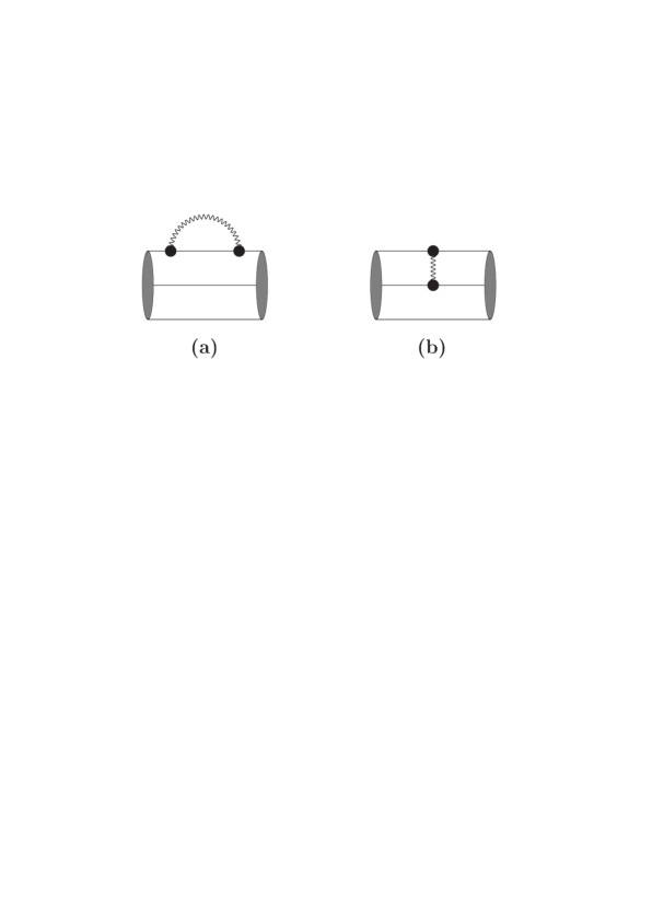
Figure 1: Electromagnetic mass shift of the nucleon.

the e.m. mass shift $\Delta m_{N}^{em}$ is generated by two diagrams: one-body (Fig.1a) and two-body diagram (Fig.1b).

The leading e.m. corrections (up to order $e^{2}/F^{2}$) to the $\pi N$ scattering amplitude at threshold are generated by the interaction Lagrangian

$${\cal L}_{I}^{W}(x)={\cal L}_{I}^{W;str}(x)+{\cal L}_{I}^{W;em}(x)$$ (7)

where ${\cal L}_{I}^{W;str}$ is given in Eq. (3) and the additional e.m. part ${\cal L}_{I}^{W;em}$ is given by

$${\cal L}_{I}^{W;em}(x) = {\cal L}^{em}(x)\,+\,\frac{e}{4F^{2}}A_{\mu}(x)\bar{\psi}(x)\gamma^{\mu}[\vec{\pi}^{\,2}(x)\tau_{3}-\vec{\pi}(x)\vec{\tau}\pi^{0}(x)]\psi(x)$$

$$- eA_{\mu}(x)\varepsilon_{3ij}\biggl{[}\pi_{i}(x)\partial^{\mu}\pi_{j}(x)\,-\,\frac{\pi_{j}(x)}{2F}\bar{\psi}(x)\gamma^{\mu}\gamma^{5}\tau_{i}\psi(x)\biggr{]}$$

The $\pi N$ amplitude in the presence of $O(e^{2})$ radiative corrections is given by

$${{}^{N}\langle}\phi_{0};\pi_{j}|\,\sum\limits_{n=1}^{4}\frac{i^{n}}{n!}\int\,d^{4}x_{1}\ldots\int d^{4}x_{n}\,\,T[{\cal L}_{I}^{W}(x_{1})\ldots{\cal L}_{I}^{W}(x_{n})\,]\,|\phi_{0};\pi_{i}{\rangle^{N}_{c}}.$$ (9)

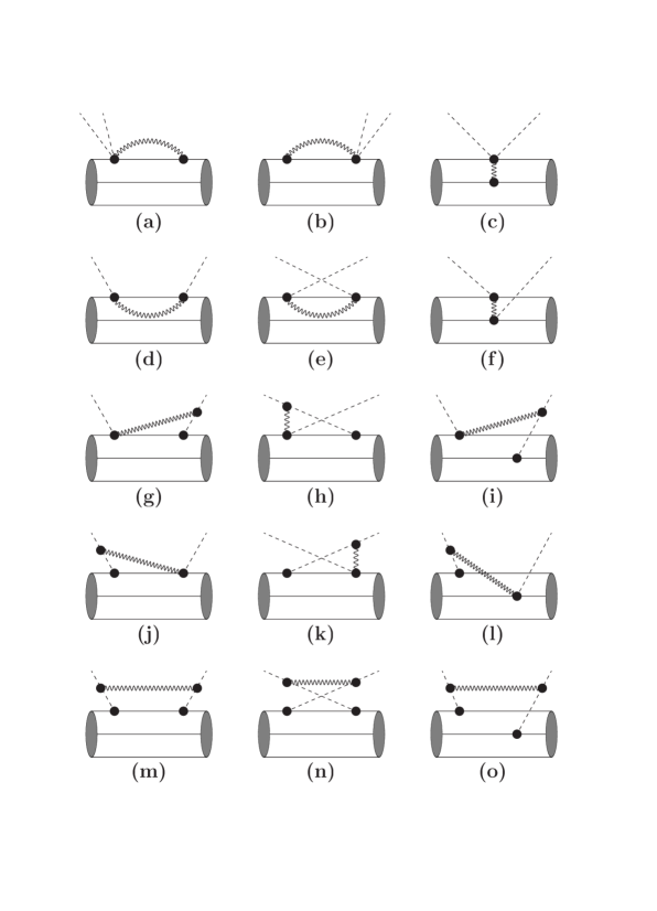
Figure 2: Leading $e^{2}/F^{2}$ radiative corrections to the $\pi N$ amplitude at threshold.

The diagrams for $O(e^{2}/F^{2})$ radiative corrections to the $\pi N$ amplitude at threshold are shown in Fig.2. To evaluate the diagrams in Figs.1 and 2 we use the photon propagator $D_{\mu\nu}$ in the Coulomb gauge to separate the contributions from Coulomb and transverse photons.

First, we analyze the e.m. mass shift of the nucleon. The contributions of diagrams Fig.1a and Fig.1b are given by

$$\Delta m^{em;a}_{N} = e^{2}\,\cdot\,{{}^{N}\langle}\phi_{0}|\int d^{4}x\int d^{4}y\,\delta(x^{0})\,D_{\mu\nu}(x-y)$$

$$\times \bar{\psi}_{0}(x)\,\gamma^{\mu}\,Q\,iG_{\psi}(x,y)\,\gamma^{\nu}\,Q\,\psi_{0}(y)\,|\phi_{0}{\rangle^{N}}$$

$$\Delta m^{em;b}_{N} = \frac{e^{2}}{2}\,\cdot\,{{}^{N}\langle}\phi_{0}|\int d^{4}x\int d^{4}y\,\delta(x^{0})\,D_{\mu\nu}(x-y)$$

$$\times \bar{\psi}_{0}(x)\,\gamma^{\mu}\,Q\,\psi_{0}(x)\,\bar{\psi}_{0}(y)\,\gamma^{\nu}\,Q\,\psi_{0}(y)\,|\phi_{0}{\rangle^{N}}.$$

where $iG_{\psi}(x,y)=<0|T\{\psi(x)\bar{\psi}(y)\}|0>$ is the quark propagator in a binding potential. In the following we truncate the expansion of the quark propagator to the ground state eigen mode:

$$iG_{\psi}(x,y)\to iG_{0}(x,y)\doteq u_{0}(\vec{x})\,\bar{u}_{0}(\vec{y})\,e^{-i{\cal E}_{\alpha}(x_{0}-y_{0})}\,\theta(x_{0}-y_{0}),$$ (11)

that is we restrict the intermediate baryon states to $N$ and $\Delta$ configurations. Inclusion of excited baryon states will be subject of future investigations. With the use of approximation (11) $\Delta m^{em;a}_{N}$ and $\Delta m^{em;b}_{N}$ reduce to

$$\Delta m^{em;a}_{N} = \frac{e^{2}}{16\pi^{3}}\langle N|\sum\limits_{i=1}^{3}(Q^{2})^{(i)}|N\rangle\int\frac{d^{3}q}{\vec{q}^{\,\,2}}\biggl{\{}[G_{E}^{p}(-\vec{q}^{\,2})]^{2}-\frac{\vec{q}^{\,\,2}}{2m_{N}^{2}}[G_{M}^{p}(-\vec{q}^{\,2})]^{2}\biggr{\}}$$

$$\Delta m^{em;b}_{N} = \frac{e^{2}}{16\pi^{3}}\int\frac{d^{3}q}{\vec{q}^{\,\,2}}\,\,\biggl{\{}\langle N|\sum\limits_{i\,\not\!=j}^{3}Q^{(i)}Q^{(j)}|N\rangle[G_{E}^{p}(-\vec{q}^{\,2})]^{2}$$

$$- \langle N|\sum\limits_{i\,\not\!=j}^{3}Q^{(i)}Q^{(j)}\vec{\sigma}^{(i)}\vec{\sigma}^{(j)}|N\rangle\,\frac{\vec{q}^{\,\,2}}{6m_{N}^{2}}[G_{M}^{p}(-\vec{q}^{\,2})]^{2}\biggr{\}},$$

where $|N\rangle$ is the SU(6) spin-flavor w.f. of the nucleon. Here we introduce the proton charge $(G_{E}^{p})$ and magnetic $(G_{M}^{p})$ form factors (f.f.) calculated at zeroth order [13] (meson cloud corrections are not taken into account) with

$$\chi^{\dagger}_{N_{s^{\prime}}}\chi_{N_{s}}G_{E}(-\vec{q}^{\,2})={{}^{N}\langle}\phi_{0}|\int d^{3}x\,\bar{\psi}_{0}(\vec{x})\,\gamma^{0}\,\psi_{0}(\vec{x})\,e^{i\vec{q}\,\vec{x}}|\phi_{0}{\rangle^{N}},$$ (13)

$$\chi^{\dagger}_{N_{s^{\prime}}}\frac{i\,[\vec{\sigma}_{N}\times\vec{q}\,]}{2m_{N}}\chi_{N_{s}}G_{M}(-\vec{q}^{\,2})={{}^{N}\langle}\phi_{0}|\int d^{3}x\,\bar{\psi}_{0}(\vec{x})\,\vec{\gamma}\,\psi_{0}(\vec{x})\,e^{i\vec{q}\,\vec{x}}|\phi_{0}{\rangle^{N}}$$

where $\chi_{N_{s}}$ is the nucleon spin w.f. and $\vec{\sigma}_{N}$ is the nucleon spin operator. Note that the contributions of Coulomb and transverse photons to the e.m. mass shifts (see Eqs. ($\pi N$ scattering and electromagnetic corrections in the perturbative chiral quark model)) are related to the nucleon charge and magnetic f.f., respectively. The sum

$$\langle N|\sum\limits_{i=1}^{3}(Q^{2})^{(i)}|N\rangle+\langle N|\sum\limits_{i\,\not\!=j}^{3}Q^{(i)}Q^{(j)}|N\rangle=\left\{\begin{array}[]{cc}1&\mbox{for}\,\,\,N=p\\ 0&\mbox{for}\,\,\,N=n\\ \end{array}\right.$$ (16)

is equivalent to the charge matrix of nucleons ($Q_{N}$ being the nucleon charge). In the limit $m_{N}\to\infty$ (when we neglect the contribution of $G_{M}^{p}$ in Eqs. ($\pi N$ scattering and electromagnetic corrections in the perturbative chiral quark model)) we obtain for the e.m. mass shifts

$$\Delta m^{em}_{N}=\Delta m_{N}^{em;a}+\Delta m_{N}^{em;b}=\frac{\alpha Q_{N}^{2}}{4\pi^{2}}\int\frac{d^{3}q}{\vec{q}^{\,\,2}}\,[G_{E}^{p}(-\vec{q}^{\,2})]^{2}$$ (17)

consistent with the result (Eq. (12.4)) of Ref. [17]. Hence, the e.m. mass shift of the neutron vanishes in the heavy nucleon limit.

In the numerical analysis we use the variational Gaussian ansatz [13] for the quark ground state wave function with the following analytical form:

$$u_{0}(\vec{x})\,=\,N\,\exp\biggl{[}-\frac{\vec{x}^{\,2}}{2R^{2}}\biggr{]}\,\left(\begin{array}[]{c}1\\ i\rho\,\vec{\sigma}\vec{x}/R\\ \end{array}\right)\,\chi_{s}\,\chi_{f}\,\chi_{c}$$ (20)

where $N=[\pi^{3/2}R^{3}(1+3\rho^{2}/2)]^{-1/2}$ is a constant fixed by the normalization condition $\int d^{3}x\,u^{\dagger}_{0}(x)\,u_{0}(x)\equiv 1$; $\chi_{s}$, $\chi_{f}$, $\chi_{c}$ are the spin, flavor and color quark wave functions, respectively. Our Gaussian ansatz contains two model parameters: the dimensional parameter $R$ and the dimensionless parameter $\rho$. The parameter $\rho$ can be related to the axial coupling constant $g_{A}$ calculated in zeroth-order (or the three quark-core) approximation:

$$g_{A}=\frac{5}{3}\biggl{(}1-\frac{2\rho^{2}}{1+\frac{3}{2}\rho^{2}}\biggr{)}.$$ (21)

Therefore, $\rho$ can be replaced by the axial charge $g_{A}$ by means of the matching condition (21). The parameter $R$ can be physically understood as the mean radius of the three-quark core and is related to the charge radius of the proton in the leading-order approximation as

$$\langle r^{2}_{E}\rangle^{P}_{LO}=\int d^{3}x\,u^{\dagger}_{0}(\vec{x})\,\vec{x}^{\,2}\,u_{0}(\vec{x})\,=\,\frac{3R^{2}}{2}\,\frac{1\,+\,\frac{5}{2}\,\rho^{2}}{1\,+\,\frac{3}{2}\,\rho^{2}}.$$ (22)

In our calculations we use the value $g_{A}$=1.25 obtained in ChPT [4]. Therefore, we have only one free parameter, that is $R$. In the numerical studies [13] R is varied in the region from 0.55 fm to 0.65 fm, which corresponds to a change of $\langle r^{2}_{E}\rangle^{P}_{LO}$ from 0.5 to 0.7 fm². The exact Gaussian ansatz (20) restricts the potentials $S(r)$ and $V(r)$ to a form proportional to $r^{2}$. They are expressed in terms of the parameters $R$ and $\rho$ (for details see Ref. [13]).

Using (20) the proton f.f. at zeroth order are determined as [13]:

$$G_{E}(-\vec{q}^{\,2}) = \exp\biggl{(}-\frac{\vec{q}^{\,2}R^{2}}{4}\biggr{)}\biggl{[}1-\frac{\vec{q}^{\,2}R^{2}}{4}\kappa\biggr{]}$$ (23)

$$G_{M}(-\vec{q}^{\,2}) = \exp\biggl{(}-\frac{\vec{q}^{\,2}R^{2}}{4}\biggr{)}2m_{N}R\,\sqrt{\kappa\biggl{(}1-\frac{3}{2}\kappa\biggr{)}},\hskip 22.76228pt\kappa=\frac{1}{2}-\frac{3}{10}g_{A}.$$

With Eq. (23) the e.m. mass shift is finally given as

$$\Delta m^{em}_{p} = \frac{\alpha}{R\sqrt{2\pi}}\biggl{[}1-\frac{\kappa}{2}+\frac{3}{16}\kappa^{2}-\frac{34}{9}\kappa\biggl{(}1-\frac{3}{2}\kappa\biggr{)}\biggr{]},$$ (24)

$$\Delta m^{em}_{n} = -\frac{\alpha}{R\sqrt{2\pi}}\frac{8}{3}\kappa\biggl{(}1-\frac{3}{2}\kappa\biggr{)},$$

where $\alpha=1/137$ is the fine structure coupling. For our set of parameters $g_{A}=1.25$ and $R=0.6\pm 0.05$ fm we get $\Delta m^{em}_{p}=0.54\pm 0.04$ MeV, $\Delta m^{em}_{n}=-0.26\pm 0.02$ MeV and $\Delta m^{em}_{n}-\Delta m^{em}_{p}=-0.8\pm 0.06$ MeV. These and the following uncertainties in our results correspond to the variation of the parameter $R$. Our predictions are in qualitative agreement with the results obtained by Gasser and Leutwyler using the Cottingham formula [17]: $\Delta m^{em}_{p}=0.63$ MeV, $\Delta m^{em}_{n}=-0.13$ MeV, $\Delta m^{em}_{n}-\Delta m^{em}_{p}=-0.76$ MeV. To compare our prediction for the e.m. mass shifts of the nucleons with the result of ChPT [6], we recall the part of the ChPT Lagrangian [6] which is responsible for radiative corrections

$${\cal L}_{ChPT}^{e^{2}}=e^{2}\bar{N}\biggl{\{}f_{1}\biggl{(}1-\frac{\vec{\pi}^{\,2}-(\pi^{0})^{\,2}}{F^{2}}\biggr{)}\,+\,\frac{f_{2}}{2}\biggl{(}\tau_{3}-\frac{\vec{\pi}^{\,2}\tau_{3}-\pi^{0}\vec{\pi}\vec{\tau}}{2F^{2}}\biggr{)}+f_{3}\biggr{\}}N.$$ (25)

The $O(p^{2})$ low-energy constants (LECs) $f_{1}$, $f_{2}$ and $f_{3}$ contain the effect of the direct quark-photon interaction. Matching our results for the nucleon mass shifts to the predictions of ChPT [6] with

$$\Delta m^{em}_{p}|_{ChPT}=-4\pi\alpha\biggl{(}f_{1}+f_{3}+\frac{f_{2}}{2}\biggr{)},\hskip 4.26773pt\Delta m^{em}_{n}|_{ChPT}=-4\pi\alpha\biggl{(}f_{1}+f_{3}-\frac{f_{2}}{2}\biggr{)}$$ (26)

we obtain following relations for the coupling constants $f_{1}$, $f_{2}$ and $f_{3}$:

$$f_{2} = -\frac{1}{2R(2\pi)^{3/2}}\biggl{[}1-\frac{29}{18}\kappa+\frac{89}{48}\kappa^{2}\biggr{]},$$ (27)

$$f_{1}+f_{3} = -\frac{1}{4R(2\pi)^{3/2}}\biggl{[}1-\frac{125}{18}\kappa+\frac{473}{48}\kappa^{2}\biggr{]}.$$

Our numerical result for $f_{2}=-8.7\pm 0.7$ MeV is in good agreement with the value of $f_{2}=-8.3\pm 3.3$ MeV [6, 14] extracted from the analysis of the elastic electron scattering cross section using the Cottingham formula [17]. For $f_{1}+f_{3}$ we get $-1.5\pm 0.1$ MeV.

We furthermore give a prediction for the separate values of $f_{1}$, $f_{3}$ and the ratio $f_{1}/f_{2}$ as deduced from our model analysis of $e^{2}$ corrections to the $\pi N$ amplitude. We denote the corresponding matrix element associated with the nucleon flavor transition $N_{1}\to N_{2}$ by $M_{N_{1}N_{2}}^{(e^{2});ij}$. In the Coulomb gauge only six diagrams (Fig.2a-2f) contribute to the radiative correction to the $\pi N$ amplitude at threshold. The contribution of the other diagrams (Fig.2g-2o) vanishes. The contributions of the different diagrams of Fig.2 are as follow:

$$M_{N_{1}N_{2}}^{(e^{2});ij}\bigg{|}_{a+b} = -\frac{e^{2}}{F^{2}}\,\cdot\,{{}^{N}\langle}\phi_{0}|\int d^{4}x\int d^{4}yD_{\mu\nu}(x-y)\bar{\psi}_{0}(x)\gamma^{\mu}$$

$$\times (T^{ij}G_{\psi}(x,y)Q+QG_{\psi}(x,y)T^{ij})\gamma^{\nu}\psi_{0}(y)|\phi_{0}{\rangle^{N}}$$

for Fig.2a and 2b where $T^{ij}=2\delta^{ij}\tau^{3}-\delta^{i3}\tau^{j}-\delta^{j3}\tau^{i}$,

$$M_{N_{1}N_{2}}^{(e^{2});ij}\bigg{|}_{c} = \frac{ie^{2}}{F^{2}}\,\cdot\,{{}^{N}\langle}\phi_{0}|\int d^{4}x\int d^{4}yD_{\mu\nu}(x-y)\bar{\psi}_{0}(x)\gamma^{\mu}$$

$$\times T^{ij}\psi_{0}(x)\bar{\psi}_{0}(y)\gamma^{\nu}Q\psi_{0}(y)|\phi_{0}{\rangle^{N}}$$

for Fig.2c,

$$M_{N_{1}N_{2}}^{(e^{2});ij}\bigg{|}_{d+e} = -\frac{e^{2}}{F^{2}}\,\cdot\,{{}^{N}\langle}\phi_{0}|\int d^{4}x\int d^{4}yD_{\mu\nu}(x-y)\bar{\psi}_{0}(x)\gamma^{\mu}\gamma^{5}$$

$$\times (\varepsilon^{3ik}\varepsilon^{3jm}+\varepsilon^{3jk}\varepsilon^{3im})\tau^{k}G_{\psi}(x,y)\gamma^{\nu}\gamma^{5}\tau^{m}\psi_{0}(y)|\phi_{0}{\rangle^{N}}$$

for Fig.2d and 2e,

$$M_{N_{1}N_{2}}^{(e^{2});ij}\bigg{|}_{f} = \frac{ie^{2}}{F^{2}}\,\cdot\,{{}^{N}\langle}\phi_{0}|\int d^{4}x\int d^{4}yD_{\mu\nu}(x-y)\bar{\psi}_{0}(x)\gamma^{\mu}\gamma^{5}$$

$$\times \varepsilon^{3ik}\varepsilon^{3jm}\tau^{k}\psi_{0}(x)\bar{\psi}_{0}(y)\gamma^{\nu}\gamma^{5}\tau^{m}\psi_{0}(y)|\phi_{0}{\rangle^{N}}$$

for Fig.2f.

Truncating the quark propagator to the ground state mode the $\pi N$ scattering amplitude at threshold including first-order radiative corrections is

$$M_{inv}^{e^{2}\pi N} = -\frac{1}{(4\pi)^{3}}\int\frac{d^{3}q}{\vec{q}^{\,\,2}}\bigg{\{}M_{f_{1}}^{\pi N}\biggl{[}[G_{E}^{p}(-\vec{q}^{\,2})]^{2}-\frac{19\vec{q}^{\,\,2}}{6m_{N}^{2}}[G_{M}^{p}(-\vec{q}^{\,2})]^{2}$$

$$+ \frac{114}{25}\frac{d^{2}_{+}(\vec{q}^{\,2})}{d^{2}_{-}(\vec{q}^{\,2})}G_{A}^{2}(-\vec{q}^{\,2})\biggr{]}+M_{f_{2}}^{\pi N}\biggl{[}[G_{E}^{p}(-\vec{q}^{\,2})]^{2}-\frac{5\vec{q}^{\,\,2}}{18m_{N}^{2}}[G_{M}^{p}(-\vec{q}^{\,2})]^{2}\biggr{]}\biggr{\}}$$

$$= -\frac{1}{8R}\frac{1}{(2\pi)^{3/2}}\biggl{\{}M_{f_{1}}^{\pi N}\biggl{[}\frac{41}{3}-\frac{115}{2}\kappa+\frac{953}{16}\kappa^{2}\biggr{]}+M_{f_{2}}^{\pi N}\,\biggl{[}1-\frac{29}{18}\kappa+\frac{89}{48}\kappa^{2}\biggr{]}\biggr{\}}.$$

where

$$M_{f_{1}}^{\pi N}=-\frac{4\pi\alpha}{F^{2}}\bar{N}\{\vec{\pi}^{\,2}-(\pi^{0})^{2}\}N\,\,\,\mbox{and}\,\,\,M_{f_{2}}^{\pi N}=-\frac{4\pi\alpha}{F^{2}}\bar{N}\{\vec{\pi}^{\,2}\tau_{3}-(\vec{\pi}\vec{\tau})\pi^{0}\}N$$

and

$$d_{\pm}(\vec{q}^{\,2})=1\pm\frac{\vec{q}^{\,2}R^{2}}{4}\frac{\kappa}{1-2\kappa}.$$

The contribution of the Coulomb photons to the amplitude $M_{inv}^{e^{2}\pi N}$ is parametrized by the proton charge form factor $(G_{E})$, transverse photons are related to the proton magnetic $(G_{M})$ and axial nucleon $(G_{A})$ f.f. where the latter is given by [13]

$$G_{A}(-\vec{q}^{\,2})=g_{A}\exp\biggl{(}-\frac{\vec{q}^{\,2}R^{2}}{4}\biggr{)}d_{-}(\vec{q}^{\,2}).$$ (33)

Again, as in the case of e.m. mass shifts, the amplitude $M_{inv}^{e^{2}\pi N}$ is gauge-independent. In ChPT the corresponding amplitude is given by [6]

$$M_{inv}^{e^{2}\pi N}|_{ChPT}=f_{1}M_{f_{1}}^{\pi N}+\frac{f_{2}}{4}M_{f_{2}}^{\pi N}.$$ (34)

Comparing of Eqs. ($\pi N$ scattering and electromagnetic corrections in the perturbative chiral quark model) and (34) we get the same expression for $f_{2}$ as already obtained from the e.m. mass shift (27). We also deduce the following relations:

$$f_{1} = -\frac{1}{8R(2\pi)^{3/2}}\biggl{[}\frac{41}{3}-\frac{115}{2}\kappa+\frac{953}{16}\kappa^{2}\biggr{]},$$

$$f_{3} = \frac{1}{8R(2\pi)^{3/2}}\biggl{[}\frac{35}{3}-\frac{785}{18}\kappa+\frac{1913}{48}\kappa^{2}\biggr{]}.$$

The predicted ratio for $f_{1}/f_{2}$ depends on only one model parameter $\rho$ (or $\kappa$) which is related to the axial nucleon charge $g_{A}$ calculated at zeroth order. In addition, the constants $f_{1}$, $f_{2}$ and $f_{3}$ depend on the size parameter $R$ of the bound quark. For our ”canonical” set of parameters, $g_{A}=1.25$ and $R=0.6\pm 0.05$ fm, used in the calculations of nucleon e.m. form factors and meson-baryon sigma terms [13] we obtain:

$$f_{1}=-19.5\pm 1.6\,\,\,\mbox{MeV},\hskip 28.45274ptf_{2}=-8.7\pm 0.7\,\,\,\mbox{MeV},$$ (35)

$$f_{3}=18\pm 1.5\,\,\,\mbox{MeV},\hskip 45.52458pt\frac{f_{1}}{f_{2}}=2.2.$$

Using these values of $f_{1}$ and $f_{2}$ we can estimate the isospin-breaking correction to the energy shift of the $\pi^{-}p$ atom in the $1s$ state. The strong energy-level shift $\epsilon_{1s}$ of the $\pi^{-}p$ atom is given by the model-independent formula [14]: $\epsilon_{1s}=\epsilon_{1s}^{LO}+\epsilon_{1s}^{NLO}=\epsilon_{1s}^{LO}(1+\delta_{\epsilon})$ where the leading order (LO) or isospin-symmetric contribution is $\epsilon_{1s}^{LO}$ and the next-to-leading order (NLO) or isospin-breaking contribution is $\epsilon_{1s}^{NLO}$. The quantity $\epsilon_{1s}^{LO}$ is expressed with the help of the well-known Deser formula [18] in terms of the $S$-wave $\pi N$ scattering lengths with $\epsilon_{1s}^{LO}=-2\alpha^{3}\mu_{c}^{2}{\cal A}_{str}$ and ${\cal A}_{str}=(2a_{\frac{1}{2}}+a_{\frac{3}{2}})/3$. The reduced mass of the $\pi^{-}p$ atom is denoted by $\mu_{c}=m_{p}M_{\pi^{+}}/(m_{p}+M_{\pi^{+}})$ and ${\cal A}_{str}=(88.4\pm 1.9)\times 10^{-3}M_{\pi^{+}}^{-1}$ is the strong (isospin-invariant) regular part of the $\pi^{-}p$ scattering amplitude at threshold [19] (for the definitions of these quantities see Ref. [14]). In ChPT the quantity $\delta_{\epsilon}$, the ratio of NLO to LO corrections, is expressed in terms of the LECs $c_{1}$, $f_{1}$ and $f_{2}$

$$\delta_{\epsilon} = \frac{\mu_{c}}{8\pi M_{\pi^{+}}F^{2}_{\pi}{\cal A}_{str}}[8c_{1}(M_{\pi^{+}}^{2}-M_{\pi^{0}}^{2})-e^{2}(4f_{1}+f_{2})]-2\alpha\mu_{c}({\rm ln}\alpha-1){\cal A}_{str}.$$ (36)

The quantity $c_{1}$ is the strong LEC from the ChPT Lagrangian [5, 7] and $F_{\pi}=92.4~{}{\rm MeV}$ is the physical value of the pion decay constant [14]. In Ref. [13] we obtained $c_{1}=-1.16\pm 0.1$ GeV^-1 using the PCQM approach. Our prediction for $c_{1}$ is close to the value $c_{1}=-0.9m_{N}^{-1}$ deduced from the $\pi N$ partial wave analysis KA84 using Baryon Chiral Perturbation Theory [7]. Substituting the central values for our couplings $f_{1}=-19.5$ MeV, $f_{2}=-8.7$ MeV and $c_{1}=-1.16$ GeV^-1 into Eq. (36), we get $\delta_{\epsilon}=-2.8\cdot 10^{-2}$. Our estimate is comparable to a prediction based on a potential model for the $\pi N$ scattering [19]:
$\delta_{\epsilon}=-2.1\cdot 10^{-2}$.

In conclusion, we give predictions for the $O(p^{2})$ electromagnetic (e.m.) low-energy couplings (LECs) $f_{1}$, $f_{2}$ and $f_{3}$ as originally set up in the ChPT effective Lagrangian. The magnitude of $f_{2}$ and its relation to $f_{1}$ and $f_{3}$ are obtained from an analysis of the nucleon e.m. mass shift and the leading radiative corrections to the $\pi N$ scattering amplitude at threshold. Using our values for $f_{1}$ and $f_{2}$ we also predict the isospin-breaking correction to the strong energy shift of the $\pi^{-}p$ atom in the $1s$ state. Latter prediction is extremely important for the ongoing experiment ”Pionic Hydrogen” at PSI, which intends to measure the ground-state shift and width of pionic hydrogen ($\pi^{-}p$-atom) at the $1\%$ level [20].

Acknowledgements. We thank A. Rusetsky for useful discussions. This work was supported by the DFG (grant FA67/25-1) and by the DAAD-PROCOPE project.

References

• [1] S. Weinberg, Phys. Rev. Lett. 17 (1966) 616.
• [2] Y. Tomozawa, Nuovo Cim. A 46 (1966) 707.
• [3] S. Weinberg, Phys. Rev. 166 (1968) 1568.
• [4] J. Gasser, M. E. Sainio, and A. B. Švarc, Nucl. Phys. B 307 (1988) 779.
• [5] N. Fettes, Ulf-G. Meissner, and S. Steininger, Nucl. Phys. A 640 (1998) 199.
• [6] G. Müller and Ulf-G. Meissner, Nucl. Phys. B 556 (1999) 265;
N. Fettes, Ulf-G. Meissner, and S. Steininger, Phys. Lett. B 451 (1999) 233.
• [7] T. Becher and H. Leutwyler, Eur. Phys. J. C 9 (1999) 643; JHEP 0106 (2001) 017.
• [8] M. Gell-Mann and M. Lévy, Nuovo Cim. 16 (1960) 1729.
• [9] A. W. Thomas, J. Phys. G 7 (1981) L283; M. A. Morgan, G. A. Miller, and A. W. Thomas, Phys. Rev. D 33 (1986) 817.
• [10] B. K. Jennings and O. V. Maxwell, Nucl. Phys. A 422 (1984) 589.
• [11] V. E. Lyubovitskij, T. Gutsche, A. Faessler, and R. Vinh Mau, in preparation.
• [12] T. Gutsche and D. Robson, Phys. Lett. B 229 (1989) 333; T. Gutsche, Ph. D. Thesis, Florida State University, 1987 (unpublished).
• [13] V. E. Lyubovitskij, T. Gutsche, A. Faessler, and E.G. Drukarev, Phys. Rev. D 63 (2001) 54026; V. E. Lyubovitskij, T. Gutsche, and A. Faessler, hep-ph/0105043.
• [14] V. E. Lyubovitskij and A. Rusetsky, Phys. Lett. B 494 (2000) 9.
• [15] A. W.  Thomas, Adv. Nucl. Phys. 13 (1984) 1; E. Oset, R. Tegen, and W. Weise; Nucl. Phys. A 426 (1984) 456; S. A. Chin, Nucl. Phys. A 382 (1982) 355.
• [16] M. Gell-Mann and F. Low, Phys. Rev. 84 (1951) 350.
• [17] J. Gasser and H. Leutwyler, Phys. Rep. 87 (1982) 77.
• [18] S. Deser, M.L. Goldberger, K. Baumann, and W. Thirring, Phys. Rev. 96 (1954) 774.
• [19] D. Sigg, A. Badertscher, P.F.A. Goudsmit, H.J. Leisi, and G.C. Oades, Nucl. Phys. A 609 (1996) 310.
• [20] D. Gotta, $\pi N$ Newslett. 15 (1999) 276.
Refer to caption