Possible $Z$-width probe of a “brane-world” scenario for neutrino masses

Abstract

The possibility that the accurately known value of the Z width might furnish information about the coupling of two neutrinos to the Majoron (Nambu-Goldstone boson of spontaneous lepton number violation) is proposed and investigated in detail. Both the “ordinary” case and the case in which one adopts a “brane” world picture with the Majoron free to travel in extra dimensions are studied. Bounds on the dimensionless coupling constants are obtained, allowing for any number of extra dimensions and any intrinsic mass scale. These bounds may be applied to a variety of different Majoron models. If a technically natural see-saw model is adopted, the predicted coupling constants are far below these upper bounds. In addition, for this natural model, the effect of extra dimensions is to decrease the predicted partial Z width, the increase due to many Kaluza-Klein excitations being compensated by the decrease of their common coupling constant.

I Introduction

At present, there are many hints that our working models of elementary particle interactions and gravity may be unified at a short distance scale by a string-type theory. The practical implementation of such ideas is conceivably “around the corner” but also probably very far off. In such a situation it makes sense to study simpler models which display some features of the string theory. Especially interesting is the (Kaluza-Klein) idea of extra dimensions and the possibility that we live on a “brane” immersed in these extra dimensions [1, 2]. It is also natural to expect that such models [3, 4, 5, 6, 7] could shed some light on the theory of massive neutrinos which seem to be reluctant participants in the so called “standard-model”. A popular assumption, which is reasonable to study in detail, is the requirement that particles carrying non-trivial $SU(3)_{c}\times SU(2)_{L}\times U(1)_{Y}$ quantum numbers and the associated gauge fields are confined to the brane while others (like the graviton) may propagate also in the extra dimensions. Many authors have thus investigated the possibility that right handed neutrinos might propagate in the extra dimensions and that their resultant suppressed couplings to the usual left handed neutrinos could account for the low scale of neutrino masses[3, 4]. A large number of authors [8, 9, 10, 11, 12] have studied the constraints on such models due to experiment and observation. An alternate approach[13], corresponding to the conventional see-saw mechanism, has also been investigated by some authors. In this approach a Higgs singlet, which carries no standard model gauge quantum numbers, is allowed to propagate in the extra dimensions and give mass to right handed neutrinos which, for simplicity, are assumed to live on the brane. This model does not automatically result in the correct neutrino mass scale, but may do so in more sophisticated versions. In any event it is interesting to study a version in which the lepton number is spontaneously broken so that a Goldstone boson called the “Majoron” is present. (See also [14])

In this paper we shall study a simple model of this type and calculate the decay rate for the intermediate vector boson $Z$ to go to two neutrinos and the Majoron (denoted by $J$) or one of its “Kaluza-Klein” excitations. Depending on the exact nature of the extra dimension scenario, there may be many such excitations so that the lepton number violating process $Z\rightarrow\nu\nu(J)$ might be expected to be large enough to, some day, be detected by a subtraction measurement. According to the latest “Review of Particle Physics”[15] the $Z$ width is:

$$\Gamma(Z)=2.4952\pm 0.0022~{}{\rm GeV}\ ,$$ (1)

and the “invisible” partial width is

$$\Gamma({\rm invisible})=499.4\pm 1.7~{}{\rm MeV}\ .$$ (2)

The uncertainties in these expressions give an idea of the partial width needed for possible detection. The related neutrinoless double beta decay process $n+n\rightarrow p+p+e^{-}+e^{-}+(J)$ has already been treated in a model of the present type [13]. A detailed discussion of supernova constraints in the 3 $+$ 1 dimensional theory has very recently been given in [16].

Section II contains a brief review of the Majoron model and also its extension to the extra dimensional brane-world picture. In section III the partial width for the lepton number violating process Z $\rightarrow$ two neutrinos plus a particular majoron excitation is expressed as an integral over phase space. The integrand is evaluated to leading order in the neutrino mass, $m_{\nu}$.In this simplifying limit, an overall factor $m_{\nu}^{2}$ carries its $m_{\nu}$ dependence. The integral itself is evaluated in section IV for this process in the usual 3 $+$ 1 dimensional theory with a single zero mass majoron. This is a little delicate since the main contribution arises from near the phase space boundary, just outside of which lurks a singularity. It proves instructive to evaluate the integral analytically. Section V contains the calculation for the partial width of Z decay to two neutrinos plus a particular majoron excitation in the extra dimensional theory. An analytic approximation of the numerically obtained rate integral, based on the approach of the previous section, permits convenient integration over the majoron tower in the general case. Finally, a brief summary is presented in section VI.

II Majoron model

First, we briefly review the original Majoron model of Chikashige, Mohapatra and Peccei [17]. It is a model for generating spontaneously the broken lepton number associated with massive Majorana neutrinos. Here, the notations of [18] will be followed. In addition to the usual Higgs doublet

$$\phi=\left(\begin{array}[]{c}\phi^{+}\\ \phi^{0}\end{array}\right)\qquad l=0$$ (3)

which has lepton number $l$ equal to zero, the model contains an electrically neutral complex singlet field

$$\Phi\qquad l=-2\ .$$ (4)

The kinetic terms of the Lagrangian are:

$$-\frac{1}{2}\partial_{\mu}\phi^{\dagger}\partial_{\mu}\phi-\frac{1}{2}\partial_{\mu}\Phi^{\ast}\partial_{\mu}\Phi\ .$$ (5)

(The factor $1/2$ is a convenient convention and we also use the Minkowski metric convention $(x_{0}=it,x_{1},x_{2},x_{3})$.) It is required that the Higgs potential constructed from $\Phi$ and $\phi$ conserves lepton number. The vacuum values are:

$$<\Phi> = <\Phi^{\ast}>=X\ ,$$ (6)

$$<\phi^{0}> = <{\phi^{0}}^{\dagger}>=\lambda\approx 2^{-\frac{1}{4}}G_{F}^{-\frac{1}{2}}\ ,$$ (7)

where $G_{F}$ is the Fermi constant and $X$ (whose non-zero value violates lepton number) sets a new scale in the theory. We assume the theory contains three two component neutrino spinors $\rho_{1},\rho_{2},\rho_{3}$ with $l=1$, belonging to $SU(2)_{L}$ doublets and three two component spinors $\rho_{4},\rho_{5},\rho_{6}$ with $l=-1$ which are singlets under $SU(2)_{L}\times U(1)_{Y}$. These are united as

$$\rho^{T}=\left(\rho_{1}^{T},\rho_{2}^{T},\rho_{3}^{T},\rho_{4}^{T},\rho_{5}^{T},\rho_{6}^{T}\right)\ ;$$ (8)

all the $\rho_{a}$ have the same Lorentz transformation property. Then the (lepton number conserving) Yukawa terms involving the neutrinos may be written as:

$${\cal L}_{yukawa}=-\frac{1}{2}\rho^{T}\sigma_{2}\left(\begin{array}[]{cc}0&\frac{\phi^{0}}{\lambda}{\cal D}\\ \frac{\phi^{0}}{\lambda}{\cal D}^{T}&\frac{\Phi^{\ast}}{X}{\cal M}_{H}\end{array}\right)\rho+{\rm h.c.}\ ,$$ (9)

where $\sigma_{2}$ is the Pauli matrix. The $3\times 3$ matrix $\frac{1}{\lambda}{\cal D}$ represents the “Dirac-type” coupling constants for the bare light neutrinos while the $3\times 3$ matrix $\frac{1}{X}{\cal M}_{H}$ represents the Majorana type coupling constants for the bare heavy (or “right handed”) neutrinos. As a whole Eq. (9) is just a generic “see-saw mechanism” [19]. It is necessary to diagonalize the matrix by a unitary transformation:

$$\rho=U\nu\ ,$$ (10)

to physical fields $\nu$. This can be carried out [18] approximately as a power series expansion in

$$\epsilon={\cal O}\left(\frac{\cal D}{{\cal M}_{H}}\right)\ .$$ (11)

We will focus attention on the three light physical neutrinos $\nu_{1},\nu_{2},\nu_{3}$. These will acquire Majorana masses $m_{1},m_{2},m_{3}$ which are of order $\epsilon^{2}{\cal M}_{H}$ (which is just the counting of the see-saw mechanism). For our present purpose we need the coupling of the Majoron $J$, identified as $J={\rm Im}\Phi$, to the physical neutrino fields $\nu_{1},\nu_{2},\nu_{3}$:

$${\cal L}_{J}=i\frac{J}{2}\sum_{a,b=1}^{3}\nu^{T}_{a}\sigma_{2}g_{ab}\nu_{b}+{\rm h.c.}\ .$$ (12)

It turns out [18] that the coupling constants have the expansion:

$$g_{ab}=-\frac{1}{X}m_{a}\delta_{ab}+{\cal O}\left(\epsilon^{4}{\cal M}_{H}\right)\ ,$$ (13)

where the leading term is seen to be diagonal in generation space. Rewriting, for convenience, this leading term using four component ordinary Dirac spinors

$$\psi_{a}=\left(\begin{array}[]{c}\nu_{a}\\ 0\end{array}\right)\ ,$$ (14)

in a $\gamma_{5}$ diagonal representation of the Dirac matrices, we get:

$${\cal L}_{J}=i\frac{J}{2X}\sum_{a=1}^{3}m_{a}\left(\psi^{T}_{a}C^{-1}\frac{1+\gamma_{5}}{2}\psi_{a}+\bar{\psi}_{a}\frac{1-\gamma_{5}}{2}C\bar{\psi}^{T}_{a}\right)\ .$$ (15)

Here $C$ is the charge conjugation matrix of the Dirac theory.

Now let us consider how this treatment gets modified when we allow the singlet field $\Phi$ to propagate in $\delta$ extra spatial dimensions. These extra dimensions, denoted as $y_{i}$ with $i=1,\ldots\delta$, will be assumed to be toroidally compactified via the identification $y_{i}=0$ and $y_{i}=2\pi R_{i}$. For simplicity all $R_{i}$ will be taken equal to the same value $R$. It is convenient to take $\Phi\left(x,y\right)$ to continue to carry the “engineering dimension” one as it would in $3+1$ dimensional space-time. Then the kinetic term of the dimensionless action in $(3+\delta)+1$ space-time

$$S=-\frac{1}{2}\int d^{4}xd^{\delta}y\,M^{\delta}_{S}\,\partial_{\mu}\Phi^{\ast}\partial_{\mu}\Phi\ ,$$ (16)

includes a rescaling mass $M_{S}$ which represents the intrinsic scale of the resulting theory. With a Fourier expansion with respect to the compactified coordinates

$$\Phi\left(x,y\right)={\rm Norm}\sum_{n_{1},n_{2},\ldots,n_{\delta}}\Phi_{n_{1},n_{2},\ldots,n_{\delta}}\left(x\right)\exp\left[\frac{i}{R}\left(n_{1}y_{1}+n_{2}y_{2}+\cdots\right)\right]\ ,$$ (17)

up to an additive constant where ${\rm Norm}=\left[2\pi M_{S}R\right]^{-\frac{\delta}{2}}$, the kinetic action reads

$$S=-\frac{1}{2}\int d^{4}x\,\left[\partial_{\mu}\Phi^{\ast}_{n_{1},n_{2},\ldots}(x)\partial_{\mu}\Phi_{n_{1},n_{2},\ldots}(x)+\frac{1}{R^{2}}\left(n_{1}^{2}+n_{2}^{2}+\cdots\right)\Phi_{n_{1},n_{2},\dots}^{\ast}(x)\Phi_{n_{1},n_{2},\ldots}\right]\ .$$ (18)

This expression with

$$\Phi_{n_{1},n_{2},\ldots}(x)={\rm Re}\Phi_{n_{1},n_{2},\ldots,}(x)+i\,J_{n_{1},n_{2},\ldots}(x)\ ,$$ (19)

shows that each Kaluza-Klein (i.e. Fourier component) field receives a mass squared increment

$$\Delta m^{2}_{n_{1},n_{2},\ldots}=\frac{1}{R^{2}}\left(n_{1}^{2}+n_{2}^{2}+\cdots n_{\delta}^{2}\right)\ .$$ (20)

The true, zero-mass, Majoron is $J_{0,0,\ldots,0}(x)$ and will receive no other mass squared increment. However the fields ${\rm Re}\Phi_{n_{1},n_{2},\ldots}(x)$ will receive a substantial increment from the pure Higgs sector of the theory.

Note that the normalization constant introduced in (17) involves the two quantities: intrinsic scale $M_{S}$ and compactification radius $R$. These are related to each other if it is assumed that the “brane” model allows the graviton to propagate in the full $(3+\delta)+1$ dimensional space-time. Then the ordinary form of Newtons’ gravitation law is only an approximation valid at distances much greater than $R$. The Newtonian gravitational constant (inverse square of the Planck mass $M_{P}$) is obtained [1] as a phenomenological parameter from

$$\left(\frac{M_{P}}{M_{S}}\right)^{2}=\left(2\pi M_{S}R\right)^{\delta}=\frac{1}{\left(\rm Norm\right)^{2}}\ .$$ (21)

Considering $M_{P}$ as an experimental input (and approximating $R_{1}=R_{2}=\cdots=R_{\delta}$), shows via (21) that $M_{S}$ is the only free parameter introduced to describe the extra dimensional aspect of the present simple theory when $\delta$ is fixed.

Next consider the Higgs “potential” for the extended theory. For simplicity we assume that the lepton conserving overlap term $\Phi^{\ast}\Phi\phi^{\dagger}\phi$ is negligible. Then the Higgs potential for the normal Higgs field $\phi$ is the same as in the standard model while the Higgs potential for $\Phi$ is described by the action

$$-\int d^{4}xd^{\delta}y\,\left[-c_{0}M_{S}^{\delta+2}\Phi^{\ast}\Phi+c_{1}M_{S}^{\delta}\left(\Phi^{\ast}\Phi\right)^{2}\right]\ ,$$ (22)

where $\Phi$, as before, has engineering dimension equal to one. The quantities $c_{0}$ and $c_{1}$ are positive (for spontaneous breakdown of lepton number) and dimensionless. One might expect $c_{0}$ and $c_{1}$ to be very roughly of order unity. The minimization of (22) leads to the vacuum value

$$X\equiv\langle\Phi\rangle=\sqrt{\frac{c_{0}}{2c_{1}}}M_{S}\ .$$ (23)

We also find from (22) the increment to be added to (20) for the ${\rm Re}\Phi_{n_{1},n_{2},\ldots}(x)$ fields:

$$\Delta m^{2}_{n_{1},n_{2},\ldots}\left({\rm Re}\Phi_{n_{1},n_{2},\ldots}\right)=2c_{0}M^{2}_{S}\ .$$ (24)

This result suggests that the ${\rm Re}\Phi_{n_{1},n_{2},\ldots}$ fields are too heavy to be produced by $Z$ decays. Finally, consider the neutrino Yukawa terms in the extended theory. The interactions of the usual Higgs field $\phi$ in (9) do not change in the present model. However the lower right sub-block of the matrix in (9) should now be gotten from the action piece:

$$-\frac{1}{2}\int d^{4}xd^{\delta}y\,\rho^{T}_{a}(x)\,\sigma_{2}\,\frac{{{\cal M}_{H}}_{ab}}{X}\,\rho_{b}(x)\Phi^{\ast}(x,y)\delta^{\delta}(y)+{\rm h.c.}\ ,$$ (25)

where ${{\cal M}_{H}}_{ab}/X$ is a matrix of Yukawa coupling constants and the indices ($a,b$) go over only those for the heavy singlet neutrinos ($4,5,6$). $\Phi(x,y)$ has the decomposition

$$\Phi(x,y)=X+\frac{M_{S}}{M_{P}}\sum_{n_{1},n_{2},\ldots}\Phi_{n_{1},n_{2},\ldots}(x)\exp\left[\frac{i}{R}\left(n_{1}y_{1}+n_{2}y_{2}+\cdots\right)\right]\ ,$$ (26)

where (21) was used. Substituting (26) into (25) shows, first, that the physical light neutrinos have masses of the order (via the see-saw mechanism)

$$\frac{{\cal D}^{2}}{M_{S}\sqrt{\frac{c_{0}}{2c_{1}}}\left(\frac{{\cal M}_{H}}{X}\right)}\ ,$$ (27)

where ${\cal M}_{H}/X$ is expected to be very roughly of the order unity. Secondly, the Yukawa interactions of the Majoron and its Kaluza-Klein excitations with the light neutrinos are described by (c.f. (15)):

$${\cal L}_{J}=\sum_{a=1}^{3}\sum_{n_{1},n_{2},\ldots}\frac{i}{2X}\frac{M_{S}}{M_{P}}J_{n_{1},n_{2},\ldots}m_{a}\left(\psi^{T}_{a}C^{-1}\frac{1+\gamma_{5}}{2}\psi_{a}+\bar{\psi}_{a}\frac{1-\gamma_{5}}{2}C\bar{\psi}^{T}_{a}\right)\ ,$$ (28)

to leading order in the neutrino masses, $m_{a}$.

III $Z\rightarrow\nu\nu(J)$ decay

This conceivable future test of a Majoron propagating in extra dimensions is the focus of our present interest. Now we calculate the amplitude for the $Z$ intermediate vector boson to decay into two particular neutrinos and a given member $J_{n_{1},...,n_{\delta}}$ of the Majoron Kaluza-Klein tower. The Feynman diagram is shown in Fig. 1.

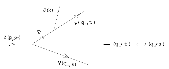
FIG. 1.: Feynman diagram for $Z\rightarrow\nu\nu J$

The crucial coupling constant for the lepton number violating $(J)\nu\nu$ vertex in the present model is read off from (28) and (23) as

$$g_{a,b;n_{1}...n_{\delta}}=-\sqrt{\frac{2c_{1}}{c_{0}}}\>\frac{m_{a}}{M_{p}}\delta_{ab},$$ (29)

correct to order $m_{a}$. Of course, our treatment could be applied to any other Majoron model if $g$ in (29) is appropriately modified. We also need the usual $Z\bar{\nu}\nu$ coupling term of the standard model:

$${\cal L}_{Z\bar{\nu}\nu}=\frac{-ie}{sin(2\theta_{W})}Z_{\mu}\sum_{a=1}^{3}\bar{\psi}_{a}\gamma_{\mu}(\frac{1+\gamma_{5}}{2})\psi_{a},$$ (30)

where e is the magnitude of the electron charge and $\theta_{W}$ is the weak mixing angle. Then the desired amplitude is

$$amp(Z\rightarrow\nu_{a}\nu_{a}J_{n_{1},...,n_{\delta}})=\frac{-e}{\sin(2\theta_{W})}g_{aa;n_{1},...,n_{\delta}}\>{\varepsilon}^{r}_{\mu}(\vec{p})\times$$ (31)

$$\bigg{[}\frac{1}{(q_{1}+k)^{2}}\bar{u}^{s}(\vec{q}_{2}){\gamma}_{\mu}(\frac{1+\gamma_{5}}{2}){\gamma}\cdot(q_{1}+k)C\bar{u}^{tT}(\vec{q}_{1})-(q_{1},t)\leftrightarrow(q_{2},s)\bigg{]},$$ (32)

(33)

correct to leading order in the neutrino mass $m_{a}$. Here $\varepsilon_{\mu}^{r}(\vec{p})$ is the Z polarization vector while the other notations are shown in Fig. 1. Note that all the neutrinos in (33) are being treated kinematically as two component massless ones even though they should describe massive Majorana fields. This is justified since the coupling $g_{a,b;n_{1}...n_{\delta}}$ already contains a factor $m_{a}$ and the corrections introduced by using the massive neutrino propagator and spinors would be higher order in $m_{a}$ and hence negligible.

We next take the squared magnitude of the amplitude (33) averaged over Z polarizations. To leading order in $m_{a}$, only one polarization state for each neutrino is needed in the calculation. After some calculation, we find the following result, expressed in the Z rest frame:

$$\frac{1}{3}\sum_{Zpol.}\mid amp(Z\rightarrow\nu_{a}\nu_{a}J_{n_{1},...,n_{\delta}})\mid^{2}=\frac{e^{2}g_{aa;n_{1},...n_{\delta}}^{2}}{12sin^{2}(2\theta_{W})}{\cal F}(E_{1},E_{2}),$$ (34)

where

$${\cal F}(E_{1},E_{2}) = \frac{E_{1}E_{2}}{m_{Z}^{2}}\Bigg{[}\frac{1}{(m_{Z}-2E_{2})^{2}}\bigg{(}8E_{2}(1-c)(E_{2}-m_{Z})+2m_{Z}^{2}(3+c)\bigg{)}$$ (35)

$$+ \frac{1}{(m_{Z}-2E_{1})^{2}}\bigg{(}8E_{1}(1-c)(E_{1}-m_{Z})+2m_{Z}^{2}(3+c)\bigg{)}$$ (36)

$$- \frac{2}{(m_{Z}-2E_{1})(m_{Z}-2E_{2})}\bigg{(}8E_{1}E_{2}c(c-1)+4m_{Z}(E_{1}+E_{2})(c-1)$$ (37)

$$+ 2m_{Z}^{2}(3+c)\bigg{)}\Bigg{]}.$$ (38)

In this formula, $E_{1}$ and $E_{2}$ are the energies of neutrino $1$ and neutrino $2$, while $c$ is the cosine of the angle between their momenta. One has

$$c=\frac{1}{2E_{1}E_{2}}[m_{Z}^{2}-m_{J}^{2}+2E_{1}E_{2}-2m_{Z}(E_{1}+E_{2})],$$ (39)

where of course the neutrino masses have been taken to be zero. ${\cal F}(E_{1},E_{2})$ is seen to be invariant under the interchange of $E_{1}$ and $E_{2}$. Finally the decay width, to particular neutrinos and excited Majoron is given by:

$$\Gamma(Z\rightarrow\nu_{a}\nu_{a}J_{n_{1}...n_{\delta}})=\frac{e^{2}g_{aa}^{2}}{48(2\pi)^{3}sin^{2}(2\theta_{W})}\frac{1}{m_{Z}}\int dE_{1}dE_{2}{\cal F}(E_{1},E_{2}).$$ (40)

To get the total contribution to the Z width we must sum over all three neutrinos and over all kinematically allowed Majoron excitations. In addition we should double the result for the inclusion of $Z\rightarrow\bar{\nu}\bar{\nu}J.$

IV $Z\rightarrow\nu\nu J$ decay in $3+1$ Majoron models

The partial width for $Z\rightarrow\nu\nu J$ in “usual” 3+1 dimensional Majoron models is expected to be small and, probably for this reason, does not seem to have been previously treated. Thus it is of some interest to present this case first. We will also see that it provides a useful “warm up” for the higher dimensional situation.

In the present case we can use the formulas of the last section and just disregard the excited Majoron states. There is only a zero mass Majoron. Our job is to numerically integrate (40) with integrand (38). In addition we should set $m_{J}$ to zero in (39). Incidentally, the phase space boundary for integration is gotten by setting $\mid c\mid=1$. The resulting boundary is shown in Fig. 2.

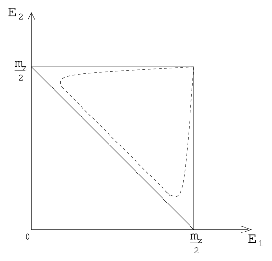
FIG. 2.: Phase space boundary for $m_{J}=0$. The solid triangular region shows the $m_{\nu}=0$ boundary, while the dashed curve is a rough sketch of the $m_{\nu}\neq 0$ case

The simple triangular region corresponds to the plausible kinematic approximation of zero neutrino masses. Now we can see that there is a problem with this approximation; the denominators in (38) vanish on the boundary lines $E_{1}=m_{Z}/2$, $E_{2}=m_{Z}/2$. To handle this we solve for the phase space boundary including the effect of non-zero neutrino mass. Generalizing (39) and setting the new $\mid c\mid$ equal to unity yields, to leading order in $m_{\nu}$, the three components of the boundary curve:

$$E_{2} = \frac{m_{Z}}{2}-m_{\nu}^{2}\bigg{(}\frac{m_{Z}-2E_{1}}{4E_{1}m_{Z}}\bigg{)}+\cdots,$$ (41)

$$E_{1}+E_{2} = \frac{m_{Z}}{2}+m_{\nu}^{2}\bigg{(}\frac{m_{Z}}{4E_{1}(m_{Z}-2E_{1})}\bigg{)}+{\cdots},$$ (42)

$$E_{1} = \frac{m_{Z}}{2}-m_{\nu}^{2}\bigg{(}\frac{m_{Z}-2E_{2}}{4E_{2}m_{Z}}\bigg{)}+{\cdots}.$$ (43)

This boundary, which is symmetric about the line $E_{1}=E_{2}$, is sketched in Fig.2, wherein the deviation from the triangular boundary is greatly exaggerated for clarity. Only at the single point $E_{1}=E_{2}=m_{Z}/2$ does the true boundary coincide with the triangular boundary. Except for this point there is no possibility of a divergence. Physically, this point corresponds to the Majoron carrying vanishing energy and the two neutrinos coming off back to back.

To go further, we simplify the expression obtained by substituting (39) into (38) with $m_{J}=0$, to find:

$${\cal F}(E_{1},E_{2})\arrowvert_{m_{J}=0}=2\bigg{(}\frac{E_{1}-m_{Z}/2}{E_{2}-m_{Z}/2}+\frac{E_{2}-m_{Z}/2}{E_{1}-m_{Z}/2}\bigg{)}+8\bigg{(}\frac{E_{1}}{m_{Z}}+\frac{E_{2}}{m_{Z}}-1\bigg{)}.$$ (44)

From this expression we see that ${\cal F}$ can be consistently defined to be finite at $E_{1}=E_{2}=m_{Z}/2$ so there is really no divergence anywhere in the physical region. Because of its simple form it is straightforward to analytically integrate (44) within the approximate boundary (43) to obtain the partial $Z$ width for a particular$J\nu_{a}\nu_{a}$ final state:

$$\Gamma(Z\rightarrow\nu_{a}\nu_{a}J)\approx\frac{e^{2}g_{aa}^{2}m_{Z}}{48(2\pi)^{3}sin^{2}(2\theta_{W})}\left[\ln\left(\frac{m_{Z}}{m_{a}}\right)-\frac{4}{3}\right].$$ (45)

For sensible values of the neutrino masses $m_{a}\leq 1\>eV$, the $\ln$ term is the dominant one. We see that the rate vanishes as $m_{a}\rightarrow 0$ since (13) shows that $g_{aa}^{2}=m_{a}^{2}/X^{2}$ and this factor overcomes the potentially troublesome $\ln(m_{a})$. In the Majoron model discussed in section 2, $m_{a}=0$ corresponds to a phase of the theory in which lepton number in not spontanously broken and the field $J=\textrm{I}m\Phi$ is not massless.

Using the well known experimental numbers for $e^{2}$, $m_{Z}$ and $\theta_{W}$ in (45) together with a choice $m_{a}\approx 1eV$ for all three $\nu_{a}$’s and all three $\bar{\nu_{a}}$’s gives the following estimate for the partial width associated with $Z\rightarrow J+2\>\textrm{neutrinos}$:

$$\Gamma(Z\rightarrow J+2\>\textrm{neutrino}s)\approx 0.14\>g_{aa}^{2}\quad GeV.$$ (46)

Comparing this with the uncertainty in the invisible width of the $Z$ quoted in (2) gives a rough bound on the coupling constant for the Majoron with two neutrinos:

$$\mid g_{aa}\mid\leq 0.11.$$ (47)

Here, of course, the assumption has been made that known decays can accurately account for the central value. This assumption, as well as the uncertainty itself, should improve in the future. As expressed in (47), the experimental bound on $\mid g_{aa}\mid$ can be applied to a more general Majoron theory (e.g., one with an arbitrarily more complicated Higgs sector) than the one given in section 2). In the present case, the bound (47) is very weak since $g_{aa}=\frac{m_{a}}{X}\approx 10^{-13}$, if X is generously chosen to be only as large as $10^{4}\,GeV$. In the extra dimensional version of the Majoron theory the invisible width is expected to be greatly increased due to the large number of extra channels with excited Majorons $J_{n_{1},n_{2},...,n_{\delta}}$. This might be expected to greatly strengthen the bound in certain scenarios.

V $Z\rightarrow\nu\nu(J)$ decay in $(3+\delta)+1$ Majoron models

Now it is necessary to consider the decay to each $J_{n_{1},...,n_{\delta}}$ and then sum them all up. The rate for each separate mode is given by (40) wherein the $m_{J}^{2}$ term in (39) is no longer neglected. The phase space boundary curve which replaces (43) now has the components:

$$E_{2}=\frac{m_{Z}}{2}-\frac{m_{J}^{2}}{2m_{Z}-4E_{1}}\ ,\qquad E_{1}+E_{2}=\frac{m_{Z}^{2}-m_{J}^{2}}{2m_{Z}}\ .$$ (48)

Here the neutrino masses have been neglected. It is easy to see that the lines $E_{1}=m_{Z}/2$ and $E_{2}=m_{Z}/2$, where the expression (38) blows up, lie outside the present phase space boundary so there is no question of a divergence. The situation is formally similar to the massive photon method of regulating the infra red divergent diagrams in QED. However the non-zero mass for $J$ is not an artifice here. For the case of the ground state $J_{0,...,0}$ of zero mass, the neutrino mass must strictly speaking be restored as in the last section.

We have carried out a numerical integration of the factor $\int dE_{1}dE_{2}{\cal F}(E_{1},E_{2})$ in (40) for relevant values of $m_{J}$ with the phase space boundary of (48) above. The results are graphed in Fig. 3. It is seen that for smaller values of $m_{J}$ (less than about $10$ GeV) the integral is a straight line function of $\ln(m_{J})$, while for large $m_{J}$ it is very small, quickly vanishing as $m_{J}\rightarrow m_{Z}$.

FIG. 3.: Plot of the integral in (40) vs $Log_{10}(m_{J}\textrm{in GeV})$

The small $(m_{J}/m_{Z})$ dependence of the integral may be understood in the following way. On substituting (39) into (38) we find that the effect of $m_{J}\neq 0$ is simply to add to the $m_{J}=0$ expression (44), pieces which vanish at least as fast as $m_{J}^{2}$. Thus for small $m_{J}$ it should be a good approximation to still use (44) for the integrand. Then, analogously to the previous section, it is straightforward to analytically integrate (44) over the phase space boundary (48) (with lower limits of the integration energies around $m_{\nu}\approx 1eV$). This yields for small $m_{J}/m_{Z}$;

$$\int dE_{1}dE_{2}{\cal F}(E_{1},E_{2})\approx m_{Z}^{2}\left[\ln\left(\frac{m_{Z}}{m_{J}}\right)-{\cal O}(1)\right]$$ (49)

where the ln term is dominant. Comparison with (45), obtained with the same integral but with the different boundary (43), is instructive. Most of the contribution to the integral comes from $E_{1}$ and $E_{2}$ close to the singularities $E_{1}=m_{Z}/2$ and $E_{2}=m_{Z}/2$ lying just outside the physical phase space boundary. In the case of (45), $m_{\nu}$ specifies the closeness of the unphysical singularity while $m_{J}$ takes over this role in the case of (49).

To go further it is convenient to make a fairly realistic analytic approximation to the “exact” numerical result illustrated in Fig. 3. Since the rate integral is very small beyond $m_{J}\approx 10$ GeV the simplest procedure is to just set it to zero beyond a certain point and use the form (49) for the main region:

$$\int dE_{1}dE_{2}{\cal F}(E_{1},E_{2})\approx\left\{\begin{array}[]{ll}m_{Z}^{2}[\ln(\frac{m_{Z}}{m_{J}})-A]&\textrm{if $\ln(\frac{m_{Z}}{m_{J}})>A$}\\ 0&\textrm{if $\ln(\frac{m_{Z}}{m_{J}})<A$}\end{array}\right.$$ (50)

The parameter choice $A\approx 1.75$, which corresponds to a cut off of $m_{J}\approx 15.8$ GeV, gives a good fit to the main low $m_{J}$ region.

We next must sum over the rates for each $m_{J}$. The members of the Majoron tower are labeled by integers $n_{1},...,n_{\delta}$ and have squared masses given by (20). In the interesting case of relatively low intrinsic scale, $M_{S}$ there are a huge number of them. For example, using (21) to relate $R$ to $M_{S}$, shows that with $M_{S}=10^{4}$ GeV and $\delta=1$, the first Majoron excitation will have a mass of order $10^{-26}$ GeV. Thus we can safely replace summation by integration. Denoting $\Gamma_{Z}(m_{J})$ as the $Z$ width to two neutrinos plus a Majoron excitation, the width for decay to the whole Majoron tower is then

$$\Gamma(Z\rightarrow\nu\nu(J)+\bar{\nu}\bar{\nu}(J))=\frac{2\pi^{\delta/2}}{\Gamma(\delta/2)}R^{\delta}\int_{0}^{m_{Z}}m_{J}^{\delta-1}\Gamma_{Z}(m_{J})dm_{J},$$ (51)

where the prefactor is associated with the “area” of a unit hypersphere in the $\delta$ dimensional space needed to count the degenerate modes in (20). $\Gamma(\delta/2)$ is the gamma function. With the approximation (50) it is simple to do the integration in (51) analytically and get the final result:

$$\Gamma(Z\rightarrow\nu\nu(J)+\bar{\nu}\bar{\nu}(J)) \approx \frac{e^{2}g_{aa}^{2}m_{Z}}{64\pi^{3}\sin^{2}(2\theta_{W})}\left[\frac{2\pi^{\delta/2}}{\Gamma(\delta/2)(2\pi)^{\delta}}\right]\left[\frac{M_{P}}{M_{S}}\right]^{2}\,\frac{1}{\delta^{2}}\left(\frac{m_{Z}}{M_{S}}e^{-a}\right)^{\delta}.$$ (52)

In obtaining this form we used (40) and also (21) (for eliminating $R$ in favor of $M_{S}$ and $\delta$). Eq. (52) can quickly give an idea of how the rate depends on the choice of $\delta$, the number of extra dimensions, and $M_{S}$, the intrinsic mass scale. Note that $A\approx 1.75$ is not an arbitrary parameter but is associated with the approximation to the exact numerical integration given in (50). $g_{aa}$, the coupling constant of each member of the Majoron tower to two neutrinos, will at first be regarded as a quantity to be bounded by comparison with experiment.

Comparing (52) with the result (45) for the Majoron model in $3+1$ dimensional space-time shows that, for the same coupling constant $g_{aa}$, there may be a big amplification factor $(\frac{M_{P}}{M_{S}})^{2}$. If $M_{S}$ is chosen to be $10^{4}GeV$, corresponding to the range which should be probed in the next generation of accelerators, this amplification factor is about $10^{30}$. It is due to the large value of the compactification radius which results in a very large number of closely spaced states in the Kaluza Klein tower. For example with $M_{S}=10^{4}GeV$ and $\delta=1,2,3,4$ we have respectively $R=2.37\times 10^{25}GeV^{-1}(4.58\times 10^{9}m),1.94\times 10^{10}GeV^{-1}(3.82\times 10^{-6}m),1.3\times 10^{5}GeV^{-1}(3.57^{-11}m),5.57\times 10^{2}GeV^{-1}(1.10\times 10^{-13}m)$. The first excited Majoron has a mass, from (20), $R^{-1}$. It is well known that $\delta\approx 1$ is ruled out for a model of this type since $R$ is evidently large enough to contradict Newton’s gravtational force law. Eq(52) shows that, when $M_{S}$ is fixed, the main dependence on $\delta$ is due to the factor $(m_{Z}/M_{S})^{\delta}$.

Substituting numbers into (52) gives for $\delta=1,2,3,4$ the respective predicted widths (in $GeV$) $4.53\times 10^{24}g_{aa}^{2}$, $8.97\times 10^{20}g_{aa}^{2}$, $2.01\times 10^{17}g_{aa}^{2}$, $4.48\times 10^{13}g_{aa}^{2}$. If the uncertainty of the $Z$’s invisible width $1.7\times 10^{-3}GeV$ is roughly taken as an indication of the maximum allowed value for the total width into a Majoron and two neutrinos these numbers can be interpreted as the following bounds on $\mid g_{aa}\mid$: $\mid g_{aa}\mid<1.9\times 10^{-14}$, $1.4\times 10^{-12}$, $9.2\times 10^{-11}$, $6.2\times 10^{-9}$ for $\delta=1,2,3,4$ respectively. These are much stronger bounds than the one obtained in (47) for the model in $3+1$ space-time dimensions.

We still must ask what is the natural value of $g_{aa}$ in the simple model presented in section II. According to (29) and the discussion of section II we would expect the very small value $\mid g_{aa}\mid\sim m_{\nu}/M_{P}\approx 10^{-28}$. Then the predicted width would be (for $\delta=2$) of the order $10^{-36}GeV$. This is even smaller than the order $10^{-27}GeV$ expected from (46) in the $3+1$ dimensional case. What is happening is that the $(\frac{M_{P}}{M_{S}})^{2}$ enhancement in (52) is being cancelled by a suppression factor$(\frac{M_{S}}{M_{P}})^{2}$ in $g_{aa}^{2}$. Also the last factor in (52) provides additional suppression. Of course these results can be modified if we are willing to accept (technically unnatural) fine tuning of the parameters. In (29) we would need to fine tune $c_{1}/c_{0}$ to be extremely large; this corresponds to an exceptionally small wrong sign mass squared term in the Higgs potential (22). In addition the Yukawa coupling (${\cal M}_{H}/X$) which appears in (22) would have to be fine tuned very large in order to keep the neutrino masses of correct order. It is possible that this fine tuning could be made natural in a supersymmetric version of the Majoron theory or with a special dynamical mechanism. Furthermore the singlet Majoron model in section 2 is the simplest one. Enlarging it by including more Higgs fields should also modify the coupling constants. Thus it is conceivable that extra dimensional theories could lead to enhancement of the $Z$’s partial width for decay to a Majoron tower and two neutrinos.

VI Summary

We investigated the possibility that the accurately known value of the Z width might be used to get information about the process Z $\rightarrow$ J $+$ two neutrinos. Here J is a Majoron– the Goldstone boson associated with a proposed mechanism for generation of neutrino mass by spontaneous breakdown of lepton number. It was noted that the main contribution to the process comes from the kinematical region near the phase space boundary, outside of which the matrix element is singular. This led to a simple analytic form for the partial width. A bound on the dimensionless lepton number violating coupling constant $g_{aa}$ of the Majoron to two neutrinos was estimated to be $\mid g_{aa}\mid\leq 0.11$. However in the simple singlet Majoron theory discussed in section II, the expected magnitude is more like $\mid g_{aa}\mid={\cal O}(10^{-13})$. Thus the bound is not very restrictive although it is possible that more complicated Majoron models might predict larger values for $\mid g_{aa}\mid$ .

The treatment above was generalized to the case where Physics is described by a ”brane” embedded in a space of $\delta$ extra dimensions, all toroidally compactified to radius R. In this case there are typically a very large number of excited Majorons. A simple approximate formula was derived for the width to all of the J’s plus two neutrinos for any value of $\delta$ and the intrinsic scale $M_{S}$. In the case $\delta=2$ and $M_{S}=10^{4}$ GeV the bound is estimated as $\mid g_{aa}\mid\leq 1.4\times 10^{-12}$, which appears considerably stronger than the ordinary one. However the coupling of “brane” particles to ones like the J, which can propagate in the extra dimensions, is greatly suppressed. Thus in an extra dimensional Majoron theory without special fine tuning of the parameters, the expected value of $\mid g_{aa}\mid$ is only about $10^{-28}$. The net effect of introducing extra dimensions is a suppression, rather than an enhancement, of the decay rate into two neutrinos plus a Majoron tower. If one relaxes the prescription of “no fine tuning” it is possible to obtain an enhancement. The same may be conjectured for possible alternative Majoron schemes in extra dimensions.

- [1] N. Arkani-Hamed, S. Dimopoulos and G. Dvali, Phys. Lett. B429,263(1998); Phys. Rev. D59,086004(1999).
- [2] L. Randall and R. Sundrum, Phys. Rev. Lett. 83, 3370(1999).
- [3] K. R. Dienes, E. Dudas and T. Gherghetta, Nucl. Phys.B557,25(1999).
- [4] N. Arkani-Hamed, S. Dimopoulos, G. Dvali and J. March-Russell, hep-ph/9811448.
- [5] G. Dvali and A. Y. Smirnov, Nucl. Phys. B563,63(1999).
- [6] R. Barbieri, P. Geminelli and A. Strumia, Nucl. Phys. B585,28(2000).
- [7] A. Ionnissian and J. W. F. Valle, Phys. Rev. D63,073002(2001).
- [8] A. E. Faraggi and M. Pospelov, Phys. Lett. B458,237(1999).
- [9] G. C. McLaughlin and J. N. Ng, Phys. Lett. B470,157(1999).
- [10] A. Das and O. Kong, Phys. Lett. B470,149(1999).
- [11] C. D. Carone, Phys. Rev. D61,015008(2000).
- [12] T. Banks, M. Dine and A. E. Nelson, JHEP 9906: 014(1999).
- [13] R. N. Mohapatra, A. Perez-Lorenzano and C. A. de S. Pires, Phys. Lett. B491,143(2000).
- [14] E. Ma, M. Raidal and U. Sarkar, Phys. Rev. Lett. 85,3769(2000).
- [15] Review of Particle Physics. D.E. Groom et al. Eur. Phys. J. C15,1(2000).
- [16] R. Tomas, H. Pas and J. W. F. Valle, hep-ph/0103017.
- [17] Y. Chikashige, R. N. Mohapatra and R. D. Peccei, Phys. Lett. B98,265(1981).
- [18] J. Schechter and J.W.F. Valle, Phys. Rev. D25, 774 (1982).
- [19] T. Yanagida, Proc. of the Workshop on Unified Theory and Baryon Number in the Universe, ed. by O. Sawada and A. Sugamato (KEK Report 79-18,1979), p 95; M. Gell-Mann, P. Ramond and R. Slansky in Supergravity, eds P. van Niewenhuizen and D. Z. Freedman (North Holland, 1979); R. N. Mohapatra and G. Senjanovic, Phys. Rev. Lett. 44, 912 (1980).