HD-THEP-01-33
hep-ph/0108125
August 2001

Spectral function at high temperature in the classical approximation

Abstract

At high temperature the infrared modes of a weakly coupled quantum field theory can be treated nonperturbatively in real time using the classical field approximation. We use this to introduce a nonperturbative approach to the calculation of finite-temperature spectral functions, employing the classical KMS condition in real time. The method is illustrated for the one-particle spectral function in a scalar field theory in $2+1$ dimensions. The result is compared with resummed two-loop perturbation theory and both the plasmon mass and width are found to agree with the analytical prediction.

PACS numbers: 11.10.Wx, 11.15.Kc

1 Introduction

Finite-temperature field theory has received considerable attention during recent years (see [1] for a comprehensive textbook). An important motivation is the physics of the quark-gluon plasma, currently under investigation at RHIC, as are baryogenesis and reheating after inflation in the early universe. Thermal field theory also provides a necessary reference point for the more complicated case of nonequilibrium quantum fields.

In thermal equilibrium a prominent role is played by spectral functions since other correlators can be recovered from it via the Kubo-Martin-Schwinger (KMS) periodicity condition [2]. Thermal field theory problems can therefore be reduced to a calculation of the appropriate spectral function. In particular the one-particle spectral function contains information on the quasiparticle structure of the theory, needed to describe transport properties of hot matter in the quark-gluon plasma with the help of a Boltzmann equation [3]. For the calculation of transport coefficients, such as the shear viscosity, the presence of a medium-dependent finite width in the one-particle spectral function is crucial [4]. Resummed perturbative descriptions of the equation of state of the hot QCD plasma may require a consistent inclusion of nontrivial quasiparticle spectral functions [5].

In spite of the apparent importance of spectral functions, nonperturbative computational schemes are rather scarce. A first-principle approach is offered by lattice field theory. However, the necessity to use a euclidean formulation hinders access to dynamical quantities such as spectral functions and other real-time correlators. Experience in the recovery of mesonic spectral functions in QCD from euclidean-time correlators has been gained in the last few years using the Maximum Entropy Method (MEM) [6]. At high temperature this approach becomes especially difficult due to the compactness of the euclidean-time direction. A formulation directly in real time avoids these problems. Unfortunately a fully nonperturbative approach to real-time quantum field correlators is still lacking.

At high temperature and weak coupling a nonperturbative approach to real-time quantities is provided by the classical approximation, originally proposed in the context of high-temperature sphaleron transitions and electroweak baryogenesis [8]. Indeed, at high enough temperature the infrared sector of a thermal field theory behaves classically as can be guessed from the Bose-Einstein distribution function at low spatial momenta:

$$n(\omega_{\mathbf{p}})=\frac{1}{\exp(\hbar\omega_{\mathbf{p}}/T)-1}\to\frac{T}{\hbar\omega_{\mathbf{p}}}=n_{\rm cl}(\omega_{\mathbf{p}}),\;\;\;\;\;\;\hbar\omega_{\mathbf{p}}\ll T,$$ (1)

with $\omega_{\mathbf{p}}=\sqrt{{\mathbf{p}}^{2}+m^{2}}$ and $T$ the temperature (we take $\hbar=1$ from now on). As is well known, a proper definition of classical thermal field theory requires an inherent ultraviolet cutoff, provided for instance by a spatial lattice, to regulate the Rayleigh-Jeans divergence. The importance of the interplay between the ultraviolet lattice modes and the physical infrared modes has been realized first in Ref. [9]. Much progress in the understanding of the classical approximation and quantum and classical thermal field theory has been made subsequently, both numerically [10] and analytically [11, 12, 13], culminating in Bödeker’s effective theory for hot infrared nonabelian field dynamics [14]. A recent review discussing various aspects of the classical approximation can be found in Ref. [15].

In this paper we introduce a nonperturbative approach to the calculation of spectral functions using the classical field approximation (Sec. 2). We demonstrate the method with a calculation of the one-particle spectral function in a scalar field theory in $2+1$ dimensions in Sec. 3. In Sec. 4 we calculate the resummed perturbative spectral function and contrast it with the nonperturbative numerical result. Our findings are summarized in Sec. 5. For a discussion of the classical analogue of thermal field theory for a weakly coupled scalar field we refer to Ref. [13].

2 Classical approximation

We consider an arbitrary bosonic operator $O$ and define the spectral function as $i$ times the expectation value of the commutator

$$\rho(x-y)=i\langle[O(x),O^{\dagger}(y)]_{-}\rangle.$$ (2)

The brackets denote expectation values at finite temperature $T$,

$$\langle O\rangle=\frac{1}{Z}\mbox{Tr}\,e^{-H/T}O,\;\;\;\;\;\;Z=\mbox{Tr}\,e^{-H/T},$$ (3)

where the trace is taken over the Hilbert space. Operators $O(x)=O(t,{\mathbf{x}})$ are time dependent with the time evolution determined by the hamiltonian $H$,

$$O(t,{\mathbf{x}})=e^{iHt}O(0,{\mathbf{x}})e^{-iHt}.$$ (4)

The spectral function obeys $\rho^{\dagger}(x)=-\rho(-x)$ and is, in our convention, real for an hermitian operator:

$$O^{\dagger}=O\;\;\;\;\rightarrow\;\;\;\;\rho^{\dagger}(x)=\rho(x).$$ (5)

In equilibrium two-point functions depend on the relative coordinates only and it is convenient to go to momentum space,

$$\rho(p)=\int{\rm d}^{4}x\,e^{-ip\cdot x}\rho(x),$$ (6)

where $p\cdot x=-p^{0}x^{0}+{\mathbf{p}}\cdot{\mathbf{x}}$, $p^{0}=\omega=E$ and $x^{0}=t$. We find that in momentum space $\rho(p)\equiv i\rho_{\rm im}(p)$ is purely imaginary. The imaginary part obeys $p^{0}\rho_{\rm im}(p^{0},{\mathbf{p}})>0$ and $\rho_{\rm im}(-p)=-\rho_{\rm im}(p)$.

For a straightforward discussion of the classical approximation it is convenient [13] to introduce also the Keldysh or statistical two-point function [16],

$$F(x-y)=\frac{1}{2}\langle[O(x),O^{\dagger}(y)]_{+}\rangle,$$ (7)

obeying $F^{\dagger}(x)=F(-x)$, $F^{\dagger}(p)=F(p)$. In terms of the usual Wightman functions [1],

$$G^{>}(x-y)=\langle O(x)O^{\dagger}(y)\rangle,\;\;\;\;\;\;G^{<}(x-y)=\langle O^{\dagger}(y)O(x)\rangle,$$ (8)

the spectral and statistical two-point functions read

$$\rho(x)=i\left[G^{>}(x)-G^{<}(x)\right],\;\;\;\;\;\;F(x)=\frac{1}{2}[G^{>}(x)+G^{<}(x)].$$ (9)

In equilibrium the importance of the spectral function is manifest since all two-point functions introduced above can be expressed in it, due to the KMS condition. We find in particular [13]

$$F(p)=-i\left[n(p^{0})+\frac{1}{2}\right]\rho(p),\;\;\;\;\;\;n(p^{0})=\frac{1}{\exp(p^{0}/T)-1},$$ (10)

where $n(p^{0})$ is the Bose-Einstein distribution function. This relation is exact. The question is whether the spectral function can be computed nonperturbatively.

The classical approximation allows access to nonperturbative correlation functions in real time, both in and out of thermal equilibrium. In a classical theory operators commute and the basic classical equilibrium correlation function in a bosonic (scalar) theory is given by

$$S(x-y)=\langle O(x)O^{\dagger}(y)\rangle_{\rm cl}\equiv\frac{1}{Z_{\rm cl}}\int D\pi D\phi\,e^{-H/T}O(x)O^{\dagger}(y),$$ (11)

with the classical partition function $Z_{\rm cl}=\int D\pi D\phi\,\exp(-H/T)$ and $O(x)=O[\phi(x),\pi(x)]$. This correlator is the classical equivalent of the Keldysh two-point function (7). The functional integral is over classical phase-space at some (arbitrary) initial time,

$$\int D\pi D\phi=\int\prod_{\mathbf{x}}{\rm d}\pi({\mathbf{x}}){\rm d}\phi({\mathbf{x}}),$$ (12)

weighted with the Boltzmann weight, providing initial conditions $\phi(0,{\mathbf{x}})=\phi({\mathbf{x}})$ and $\pi(0,{\mathbf{x}})=\pi({\mathbf{x}})$. The subsequent time evolution is determined from Hamilton’s equations of motion for $\phi(x)$ and $\pi(x)$. The definitions are given for a scalar field theory, but they can easily be carried over to (non)abelian gauge theories [10]. The most convenient formulation employs the temporal gauge, with the Gauss constraint imposed on the initial conditions. It is subsequently preserved by the classical equations of motion.

The classical spectral function is obtained by replacing $-i$ times the commutator in Eq. (2) with the classical Poisson brackets,

$$\rho_{\rm cl}(x-y)=-\langle\{O(x),O^{\dagger}(y)\}\rangle_{\rm cl},$$ (13)

defined with respect to the initial fields

$$\{A(x),B(y)\}=\int{\rm d}^{3}z\left[\frac{\delta A(x)}{\delta\phi({\mathbf{z}})}\frac{\delta B(y)}{\delta\pi({\mathbf{z}})}-\frac{\delta A(x)}{\delta\pi({\mathbf{z}})}\frac{\delta B(y)}{\delta\phi({\mathbf{z}})}\right].$$ (14)

Due to the formal correspondence between commutators and Poisson brackets the quantum and classical spectral function obey the same basic properties.

At first sight a calculation of the classical spectral function from the definition in terms of the Poisson bracket appears rather hard. Fortunately, in thermal equilibrium we may use the KMS condition to simplify the procedure. The classical KMS condition is based on the same principle as the usual KMS condition in a quantum theory: the thermal Boltzmann weight and the time evolution are controlled by the same hamiltonian $H$. An easy way to find the classical KMS condition is to consider the high-temperature (or $\hbar\to 0$) limit of the quantum KMS condition. The classical equivalent of Eq. (10) reads (compare Eq. (1))

$$S(p)=-i\frac{T}{p^{0}}\rho_{\rm cl}(p).$$ (15)

One may also derive this relation directly in the classical theory without reference to the quantum case [17, 13]. This leads to the classical KMS condition formulated in real space,

$$\rho_{\rm cl}(t,{\mathbf{x}})=-\frac{1}{T}\partial_{t}S(t,{\mathbf{x}}).$$ (16)

This relation will form the basis of the remainder of this paper. It allows us to calculate the spectral function in real time from a relatively easily accessible unequal-time correlation function.

3 Scalar field on the lattice

As an example we discuss the simple case of a real scalar field $\phi$ in $2+1$ dimensions with the hamiltonian

$$H=\int{\rm d}^{2}x\left[\frac{1}{2}\pi^{2}+\frac{1}{2}(\nabla\phi)^{2}+\frac{1}{2}m^{2}\phi^{2}+\frac{\lambda}{4!}\phi^{4}\right].$$ (17)

We focus on the one-particle spectral function and take $O(x)=O^{\dagger}(x)=\phi(x)$. Using Eqs. (16) and (11) we find directly

$$\rho_{\rm cl}(t,{\mathbf{x}})=-\frac{1}{T}\langle\pi(t,{\mathbf{x}})\phi(0,{\mathbf{0}})\rangle_{\rm cl}.$$ (18)

The right-hand-side of Eq. (18) can be computed numerically in a straightforward manner, as follows. The classical field theory is defined on a spatial lattice with $N\times N$ sites and lattice spacing $a$ and we use periodic boundary conditions. To solve the dynamics we use a leapfrog discretization with time step $a_{0}<a$. The canonical momenta $\pi(t+\frac{1}{2}a_{0},{\mathbf{x}})$ are defined at intermediate time steps, which suggests to use a symmetrized definition of the spectral function on the lattice

$$\rho_{{\rm cl},\rm lat}(t,{\mathbf{x}})=-\frac{1}{T}\left\langle\pi(t+\frac{1}{2}a_{0},{\mathbf{x}})\frac{1}{2}\left[\phi(0,{\mathbf{0}})+\phi(a_{0},{\mathbf{0}})\right]\right\rangle_{\rm cl}.$$ (19)

Figure 1: Classical spectral function $\rho_{\rm cl}(t,{\mathbf{0}})$ at zero momentum in real time. The inset shows the absolute value on a log scale. The temperature is $T/m=7.2$. Without loss of generality we use $\lambda/m=1$ throughout.

To generate thermal initial conditions we use the Kramers equation algorithm, a variant of the hybrid Monte Carlo method [18]. The evolution in real time is calculated using classical equations of motion. In a simulation we switch therefore between noisy evolution to create independent thermal configurations and hamiltonian evolution to calculate observables. The results presented below are obtained using 2000 independently thermalized initial configurations for each temperature. The mass scale $m$ is used as the dimensionful scale and the results presented are obtained with $N=128$, $am=0.2$ and $a_{0}/a=0.1$ (note that the finite time step affects the equal-time canonical relation $\partial_{t}\rho_{\rm cl}(t,{\mathbf{x}})|_{t=0}=\delta({\mathbf{x}})$). In a classical theory the coupling constant $\lambda$ can be scaled out of the equations of motion and the remaining dimensionless combination is $\lambda T/m^{2}$ (recall that $\lambda$ has a dimension of mass in $2+1$ dimensions). Without loss of generality we take therefore $\lambda/m=1$ throughout. Larger $T$ corresponds then to a larger effective interaction strength. In the simulations the temperature is determined from the average kinetic energy $T=a^{2}\langle\pi^{2}(t,{\mathbf{x}})\rangle_{\rm cl}$ and the temperatures we consider are such that $aT={\cal O}(1)$.

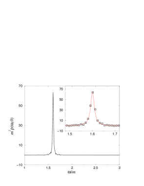
Figure 2: Spectral function $\rho_{\rm cl}(\omega,{\mathbf{0}})$, obtained from the real-time result of Fig. 1 by a sine-transform, versus the frequency $\omega$. The inset shows a magnification with the data points indicated. The dotted line is a fit to a Breit-Wigner function.

In Fig. 1 we present the classical spectral function at zero spatial momentum, obtained from a volume average of Eq. (19), in real time at a temperature $T/m=7.2$. We see oscillating approximately exponentially damped behaviour. The spectral function in frequency space can be obtained from a sine-transform

$$\rho_{{\rm cl}}(\omega,{\mathbf{p}})=2\int_{0}^{t_{\rm max}}{\rm d}t\,\rho_{{\rm cl},\rm lat}(t,{\mathbf{p}})\sin\omega t,$$ (20)

where we used the antisymmetry of the spectral function under time reflection and absorbed the $i$ of the previous section directly in the definition. The result is shown in Fig. 2. The spectral function consists of a single peak with the narrow width. The inset shows that the peak is well described by a Breit-Wigner spectral function (see Sec. 4). We have tried to find other contributions at larger frequency, but these could not be seen in the numerical data. In the numerical simulation the late-time regime becomes more and more difficult to establish, resulting typically in wiggly nondamped behaviour. This limits the time interval that can be used in the sine-transform to a maximal time $t_{\rm max}$ and constrains the resolution in frequency-space to $\Delta\omega=\pi/t_{\rm max}$. For the result in Fig. 2 the resolution is $\Delta\omega/m=\pi/300\approx 0.01$, as can be seen from the inset.

4 Perturbative expectation

The spectral function in the quantum theory can be expressed in terms of the retarded self energy $\Sigma_{R}=\mbox{Re}\,\Sigma_{R}+i\,\mbox{Im}\,\Sigma_{R}$ as [19, 20]

$$\rho_{\rm im}(\omega,{\mathbf{p}})=\frac{-2\mbox{Im}\,\Sigma_{R}(\omega,{\mathbf{p}})}{\left[\omega^{2}-{\mathbf{p}}^{2}-m^{2}-\mbox{Re}\,\Sigma_{R}(\omega,{\mathbf{p}})\right]^{2}+\left[\mbox{Im}\,\Sigma_{R}(\omega,{\mathbf{p}})\right]^{2}}.$$ (21)

The theory exhibits a quasiparticle structure, with the quasiparticle often referred to as the plasmon, in the limit that the rate $\Gamma(\omega,{\mathbf{p}})=-\mbox{Im}\,\Sigma_{R}(\omega,{\mathbf{p}})/\omega$ is much smaller than $({\mathbf{p}}^{2}+m^{2}+\mbox{Re}\,\Sigma_{R})^{1/2}$. In this case the spectral function is well approximated with a Breit-Wigner function, which at zero momentum reads

$$\rho_{\rm BW}(\omega,{\mathbf{0}})=\frac{2\omega\Gamma}{(\omega^{2}-M^{2})^{2}+\omega^{2}\Gamma^{2}}.$$ (22)

Here $M$ is the plasmon mass and $\Gamma$ its width (at zero momentum)

$$\Gamma=-\frac{\mbox{Im}\,\Sigma_{R}(M,{\mathbf{0}})}{M}.$$ (23)

In this limit contributions from multiparticle states beyond the three-particle threshold are tiny.

A perturbative calculation of the retarded self energy is standard in thermal field theory (see e.g. [20] for a clear discussion in $3+1$ dimensions). For the $(2+1)$-dimensional case we consider here we find the following. At one-loop order the tadpole diagram

$$\Sigma^{(1)}_{R}=\frac{\lambda}{2}\int\frac{{\rm d}^{2}p}{(2\pi)^{2}}\frac{n(\omega_{\mathbf{p}})+\frac{1}{2}}{\omega_{\mathbf{p}}}$$ (24)

contributes to the mass shift only. Resummation of the tadpole diagram in the limit of high temperature and weak coupling results in a gap equation for the resummed mass parameter $M$:

$$M^{2}=\frac{\lambda T}{4\pi}\log\frac{T}{M}\;\;\;\;\;\;\mbox{ (one-loop resummed)},$$ (25)

where the zero-temperature mass is neglected. In $2+1$ dimensions the one-loop mass is sensitive to both the ultraviolet momentum scale (cutoff by $T$) and the infrared momentum scale (cutoff by $M$). A finite width in the spectral function arises at two-loop order from the imaginary part of the setting-sun diagram. We focus here on on-shell $2\to 2$ scattering for which the contribution reads

$$\mbox{Im}\,\Sigma^{(2)}_{R}(\omega_{\mathbf{p}},{\mathbf{p}}) = -\frac{\lambda^{2}}{4}\int{\rm d}\Phi_{123}({\mathbf{p}})\,2\pi\delta(\omega_{\mathbf{p}}+\omega_{\mathbf{k}}-\omega_{\mathbf{q}}-\omega_{\mathbf{r}})$$

$$\times\left\{n(\omega_{\mathbf{k}})[1+n(\omega_{\mathbf{q}})][1+n(\omega_{\mathbf{r}})]-[1+n(\omega_{\mathbf{k}})]n(\omega_{\mathbf{q}})n(\omega_{\mathbf{r}})\right\},$$

with

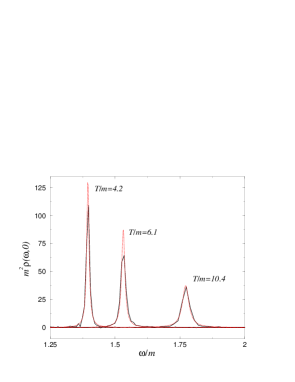
Figure 3: Spectral functions $\rho_{\rm cl}(\omega,{\mathbf{0}})$ for various temperatures $T$. Fits to a Breit-Wigner function are shown with dotted lines. The height, position and width of the peak are approximately related as $\rho_{\rm cl}(M,{\mathbf{0}})\sim 2/M\Gamma$.

$${\rm d}\Phi_{123}({\mathbf{p}})=\frac{{\rm d}^{2}k}{(2\pi)^{2}2\omega_{\mathbf{k}}}\frac{{\rm d}^{2}q}{(2\pi)^{2}2\omega_{\mathbf{q}}}\frac{{\rm d}^{2}r}{(2\pi)^{2}2\omega_{\mathbf{r}}}(2\pi)^{2}\delta({\mathbf{p}}-{\mathbf{k}}-{\mathbf{q}}-{\mathbf{r}}).$$ (26)

The on-shell dispersion relations contain the one-loop resummed mass parameter, $\omega_{\mathbf{p}}=\sqrt{{\mathbf{p}}^{2}+M^{2}}$. It is easy to check that the momentum integrals are dominated by the infrared modes. These soft modes are classical. The leading contribution at high temperature and weak coupling can therefore be obtained by replacing $n(\omega)\to T/\omega=n_{\rm cl}(\omega)$. At zero momentum ${\mathbf{p}}=0$ the integrals can be performed analytically and after a straightforward calculation we find the plasmon width in $2+1$ dimensions to be

$$\Gamma=c\frac{\lambda^{2}T^{2}}{M^{3}},\;\;\;\;\;\;c=\frac{3-2\sqrt{2}}{32\pi}\approx 0.00171.$$ (27)

In Fig. 3 the classical spectral function and fits to a Breit-Wigner function are shown for various temperatures. From the fits one may extract estimates for the classical plasmon mass and width. This provides a possibility to compare nonperturbatively determined classical plasmon masses and widths with perturbative calculations and address the applicability of one-loop resummed perturbation theory at finite temperature.

Figure 4: Mass $M_{\rm cl}$ (circles) and width $\Gamma_{\rm cl}$ (squares) of the zero-momentum spectral function as a function of the temperature. The width is multiplied with 25 for clarity. The data points are obtained from fits to a Breit-Wigner function, with the statistical error estimated from a jackknife analysis. The lines are the predictions for $M_{\rm cl}$ from the one-loop gap equation (full) and $\Gamma_{\rm cl}$ from the on-shell two-loop contribution (dashed).

The calculations in the quantum theory can easily be carried over to the classical approximation used in the numerical calculation [13]. The one-loop gap equation for the classical mass parameter $M_{\rm cl}$ reads

$$M_{\rm cl}^{2}=m^{2}+\frac{\lambda}{2}\int\frac{{\rm d}^{2}p}{(2\pi)^{2}}\frac{T}{{\mathbf{p}}^{2}+M_{\rm cl}^{2}}.$$ (28)

The integral is logarithmically divergent in the ultraviolet, which reflects the $\log T$ contribution in Eq. (25) in the quantum theory. In the classical theory the divergence is regulated by the lattice cutoff. If desired, it can be matched (renormalized) by adjusting the mass parameter $m$ in the effective classical theory [12]. In order to compare the one-loop and the nonperturbative calculation we write the gap equation on the lattice,

$$M_{\rm cl}^{2}=m^{2}+\frac{\lambda T}{2}\frac{1}{L^{2}}\sum_{n_{1},n_{2}}\frac{1}{\hat{\mathbf{p}}^{2}+M_{\rm cl}^{2}},\;\;\;\;\;\;\hat{\mathbf{p}}^{2}=\sum_{i=1}^{2}\frac{2}{a^{2}}(1-\cos ap_{i}),$$ (29)

with $p_{i}=2\pi n_{i}/L_{i}$, $-N_{i}/2+1\leq n_{i}\leq N_{i}/2$ and $L_{i}=aN_{i}=L$ ($i=1,2$), and solve it numerically. The result is presented in Fig. 4 for various temperatures. Maybe surprisingly we see that the nonperturbative determination of the plasmon mass and the resummed one-loop result differ at most a few percent, indicating the relative unimportance of higher-loop contributions for this quantity. Note that for our parameters the effective mass $M_{\rm cl}$ is small in lattice units ($aM_{\rm cl}\sim 0.3$).

An analytical expression for the width of the spectral function in the classical approximation can be obtained directly from the calculation carried out above. As indicated, the perturbative width of the spectral function in the quantum theory is dominated by soft momenta and coincides therefore with the classical result to leading order: $\Gamma_{\rm cl}$ is given by Eq. (27) after the replacement $M\to M_{\rm cl}$. A comparison between the perturbatively and nonperturbatively determined widths is presented in Fig. 4 as well. Again agreement between the two calculations can be seen, indicating that the dominant contribution is produced by the lowest order two-loop result. We emphasize that the width is a typical real-time quantity and therefore not easily accessible by other nonperturbative methods.

5 Summary

We have used the classical field approximation at high temperature and weak coupling to formulate a nonperturbative method for the calculation of spectral functions at finite temperature, with the help of the classical KMS condition. We focused on the one-particle spectral function in a scalar field theory in $2+1$ dimensions. For the temperatures investigated our numerical results indicate that the one-particle spectral function is a simple narrow peak: the spectral function is completely dominated by the plasmon. To compare with perturbation theory we calculated the one-loop resummed plasmon mass and the two-loop contribution to the width. Agreement between the nonperturbative numerical simulation and the perturbative expressions was found. These results provide a justification for the use of resummed perturbation theory for a weakly coupled scalar field in equilibrium as well as for kinetic approaches based on two-loop approximations close to equilibrium.

It would be interesting to extend the analysis to more complicated spectral functions. Transport coefficients can be expressed in terms of spectral functions of composite operators. These are in general more sensitive to the ultraviolet scale and therefore to the Rayleigh-Jeans divergence in a classical limit. Nevertheless, it might be interesting to test perturbative ideas against a nonperturbative numerical calculation. When sufficient care concerning the gauge symmetry is taken, methods applied here might also offer the possibility to gain further insight in nonperturbative aspects of hot gauge plasmas.

Acknowledgements

I would like to thank I.-O. Stamatescu for discussions and J. Berges for collaboration on related topics. This work was supported by the TMR network Finite Temperature Phase Transitions in Particle Physics, EU contract no. FMRX-CT97-0122.

References

- [1] M. Le Bellac, “Thermal Field Theory,” Cambridge University Press (1996).
- [2] R. Kubo, J. Phys. Soc. Japan 12 (1957) 570; P. C. Martin and J. Schwinger, Phys. Rev. 115 (1959) 1342.
- [3] See e.g. J. Blaizot and E. Iancu, hep-ph/0101103, and references therein.
- [4] S. Jeon, Phys. Rev. D 47 (1993) 4586 [hep-ph/9210227]; 52 (1995) 3591 [hep-ph/9409250].
- [5] J. O. Andersen, E. Braaten and M. Strickland, Phys. Rev. Lett. 83 (1999) 2139 [hep-ph/9902327]; J. P. Blaizot, E. Iancu and A. Rebhan, Phys. Rev. Lett. 83 (1999) 2906 [hep-ph/9906340].
- [6] P. de Forcrand et al. [QCD-TARO Collaboration], Nucl. Phys. Proc. Suppl. 98 (1998) 460; I. Wetzorke and F. Karsch, hep-lat/0008008; for zero temperature see M. Asakawa, T. Hatsuda and Y. Nakahara, hep-lat/0011040; T. Yamazaki et al. [CP-PACS Collaboration], hep-lat/0105030.
- [7] J. Berges and J. Cox, hep-ph/0006160, Phys. Lett. B (to appear); G. Aarts and J. Berges, hep-ph/0103049, Phys. Rev. D (to appear); J. Berges, hep-ph/0105311; G. Aarts and J. Berges, hep-ph/0107129.
- [8] D. Y. Grigoriev and V. A. Rubakov, Nucl. Phys. B 299 (1988) 67.
- [9] D. Bödeker, L. McLerran and A. Smilga, Phys. Rev. D 52 (1995) 4675 [hep-th/9504123].
- [10] J. Ambjørn and A. Krasnitz, Phys. Lett. B 362 (1995) 97 [hep-ph/9508202]; G. D. Moore, Nucl. Phys. B 480 (1996) 657 [hep-ph/9603384]; W. Tang and J. Smit, Nucl. Phys. B 482 (1996) 265 [hep-lat/9605016]; G. D. Moore and N. Turok, Phys. Rev. D 55 (1997) 6538 [hep-ph/9608350]; W. H. Tang and J. Smit, Nucl. Phys. B 510 (1998) 401 [hep-lat/9702017]; G. D. Moore, C. Hu and B. Müller, Phys. Rev. D 58 (1998) 045001 [hep-ph/9710436]; G. D. Moore and K. Rummukainen, Phys. Rev. D 61 (2000) 105008 [hep-ph/9906259]; D. Bödeker, G. D. Moore and K. Rummukainen, Phys. Rev. D 61 (2000) 056003 [hep-ph/9907545].
- [11] P. Arnold, D. Son and L. G. Yaffe, Phys. Rev. D 55 (1997) 6264 [hep-ph/9609481]; P. Arnold, Phys. Rev. D 55 (1997) 7781 [hep-ph/9701393]; D. Bödeker and M. Laine, Phys. Lett. B 416 (1998) 169 [hep-ph/9707489]; P. Arnold and L. G. Yaffe, Phys. Rev. D 57 (1998) 1178 [hep-ph/9709449]; G. Aarts, B. Nauta and C. G. van Weert, Phys. Rev. D 61 (2000) 105002 [hep-ph/9911463].
- [12] G. Aarts and J. Smit, Phys. Lett. B 393 (1997) 395 [hep-ph/9610415]; W. Buchmüller and A. Jakovác, Phys. Lett. B 407 (1997) 39 [hep-ph/9705452].
- [13] G. Aarts and J. Smit, Nucl. Phys. B511 (1998) 451 [hep-ph/9707342].
- [14] D. Bödeker, Phys. Lett. B 426 (1998) 351 [hep-ph/9801430].
- [15] D. Bödeker, Nucl. Phys. Proc. Suppl. 94 (2001) 61 [hep-lat/0011077].
- [16] L. V. Keldysh, Zh. Eksp. Teor. Fiz. 47 (1964) 1515.
- [17] G. Parisi, “Statistical Field Theory,” Addison-Wesley Publishing Company (1988).
- [18] K. Jansen and C. Liu, Nucl. Phys. B 453 (1995) 375 [hep-lat/9506020].
- [19] H. A. Weldon, Phys. Rev. D 28 (1983) 2007.
- [20] E. Wang and U. Heinz, Phys. Rev. D 53 (1996) 899 [hep-ph/9509333].