Abstract

Charginos $\tilde{\chi}^{\pm}$ and neutralinos $\tilde{\chi}^{0}$ in supersymmetric theories can be produced copiously at $e^{+}e^{-}$ colliders and their properties can be measured with high accuracy. Consecutively to the chargino system, in which the SU(2) gaugino parameter $M_{2}$, the higgsino mass parameter $\mu$ and $\tan\beta$ can be determined, the remaining fundamental supersymmetry parameter in the gaugino/higgsino sector of the minimal supersymmetric extension of the Standard Model, the U(1) gaugino mass $M_{1}$, can be analyzed in the neutralino system, including its modulus and its phase in CP–noninvariant theories. The CP properties of the neutralino system are characterized by unitarity quadrangles. Analytical solutions for the neutralino mass eigenvalues and for the mixing matrix are presented for CP–noninvariant theories in general. They can be written in compact form for large supersymmetric mass parameters. The closure of the neutralino and chargino systems can be studied by exploiting sum rules for the pair-production processes in $e^{+}e^{-}$ collisions. Thus the picture of the non–colored gaugino and higgsino complex in supersymmetric theories can comprehensively be reconstructed in these experiments.

1 Introduction

In the minimal supersymmetric extension of the Standard Model (MSSM), the spin-1/2 partners of the neutral gauge bosons, $\tilde{B}$ and $\tilde{W}^{3}$, and of the neutral Higgs bosons, $\tilde{H}_{1}^{0}$ and $\tilde{H}_{2}^{0}$, mix to form the neutralino mass eigenstates $\chi_{i}^{0}$ ($i$=1,2,3,4). The neutralino mass matrix [1] in the $(\tilde{B},\tilde{W}^{3},\tilde{H}^{0}_{1},\tilde{H}^{0}_{2})$ basis,

$${\cal M}=\left(\begin{array}[]{cccc}M_{1}&0&-m_{Z}c_{\beta}s_{W}&m_{Z}s_{\beta}s_{W}\\[5.69054pt] 0&M_{2}&m_{Z}c_{\beta}c_{W}&-m_{Z}s_{\beta}c_{W}\\[5.69054pt] -m_{Z}c_{\beta}s_{W}&m_{Z}c_{\beta}c_{W}&0&-\mu\\[5.69054pt] m_{Z}s_{\beta}s_{W}&-m_{Z}s_{\beta}c_{W}&-\mu&0\end{array}\right)\$$ (5)

is built up by the fundamental supersymmetry parameters: the U(1) and SU(2) gaugino masses $M_{1}$ and $M_{2}$, the higgsino mass parameter $\mu$, and the ratio $\tan\beta=v_{2}/v_{1}$ of the vacuum expectation values of the two neutral Higgs fields which break the electroweak symmetry. Here, $s_{\beta}=\sin\beta$, $c_{\beta}=\cos\beta$ and $s_{W},c_{W}$ are the sine and cosine of the electroweak mixing angle $\theta_{W}$. In CP–noninvariant theories, the mass parameters are complex. The existence of CP–violating phases in supersymmetric theories in general induces electric dipole moments (EDM). The current experimental bounds on the EDM’s can be exploited to derive indirect limits on the parameter space [2, 3], which however depend on many parameters of the theory outside the neutralino/chargino sector.

By reparametrization of the fields, $M_{2}$ can be taken real and positive without loss of generality so that the two remaining non–trivial phases, which are reparametrization–invariant, may be attributed to $M_{1}$ and $\mu$:

$$M_{1}=|M_{1}|\,\,{\rm e}^{i\Phi_{1}}\ \qquad{\rm and}\qquad\mu=|\mu|\,\,{\rm e}^{i\Phi_{\mu}}\qquad(0\leq\Phi_{1},\Phi_{\mu}<2\pi)$$ (6)

The experimental analysis of neutralino properties in production and decay mechanisms will unravel the basic structure of the underlying supersymmetric theory.
Neutralinos are produced in $e^{+}e^{-}$ collisions, either in diagonal or in mixed pairs [4]-[12]

$$e^{+}e^{-}\ \rightarrow\ \tilde{\chi}^{0}_{i}\ \tilde{\chi}^{0}_{j}\qquad\ \ (i,j=1,2,3,4)\,$$

If the collider energy is sufficient to produce the four neutralino states in pairs, the underlying fundamental SUSY parameters $\{|M_{1}|,\Phi_{1},M_{2},\,|\mu|,\Phi_{\mu};\tan\beta\}$ can be extracted from the masses $m_{\tilde{\chi}^{0}_{i}}$ ($i$=1,2,3,4) and the couplings. Partial information from the lowest $m_{\tilde{\chi}^{0}_{i}}$ ($i$=1,2) neutralino states [13, 3, 10] is sufficient to extract $\{|M_{1}|,\Phi_{1}\}$ in large parts of the parameter space if the other parameters have been pre–determined in the chargino sector [14, 15].

The analysis will be based strictly on low–energy supersymmetry (SUSY). To clarify the basic structure of the neutralino sector analytically, the reconstruction of the fundamental SUSY parameters is carried out at the tree level; the loop corrections [16] include parameters from other sectors of the MSSM, demanding iterative higher–order expansions in global analyses at the very end. When the basic SUSY parameters will have been extracted experimentally, they may be confronted, for instance, with the ensemble of relations predicted in Grand Unified Theories [17].

In this report we present a coherent and comprehensive description of the neutralino system, discuss its properties and describe strategies which exploit the neutralino pair production processes at $e^{+}e^{-}$ linear colliders to reconstruct the underlying fundamental theory. The report is divided into six parts. In Section 2 we extend the mixing formalism for the neutral gauginos and higgsinos to CP–noninvariant theories with nonvanishing phases. The CP properties of the neutralino mixing matrix are analysed in detail; the structure of the neutralino mixing matrix is characteristically different from the well-known CKM and MNS mixing matrices due to the Majorana nature of the fields involved. Analytic solutions for neutralino masses and mixing matrix elements are provided for the general case, and in compact form for the limit of large supersymmetry mass parameters $M_{1,2}$ and $\mu$. The special toy case $M_{1}=M_{2}$ and $\tan\beta=1$ can be solved exactly, and it illustrates the complex structure of CP violation in the neutralino system. In Section 3 the cross sections for neutralino production with polarized beams, and the polarization vectors of the neutralinos are given [9, 11]. The rise of excitation curves near threshold for non–diagonal pair production is altered qualitatively in CP–noninvariant theories. Thus, precise measurements of the threshold behavior of the non–diagonal neutralino pair production processes may give first indications of non–zero CP violating phases. In Section 4 we describe the phenomenological analysis of the complete set of the chargino and neutralino states which allows to extract the fundamental SUSY parameters in a model–independent way, leading to an unambiguous determination of the U(1) and SU(2) gaugino and higgsino parameters. The case in which the analysis is restricted to the light neutralino states $\tilde{\chi}^{0}_{1,2}$ will also be discussed. In Section 5 sum rules for the neutralino cross sections are formulated as an experimental check of the closure of the four-state neutralino system. Conclusions are finally given in Section 6.

2 Mixing formalism

2.1 General analysis

In the MSSM, the four neutralinos $\tilde{\chi}^{0}_{i}$ $(i={1,2,3,4})$ are mixtures of the neutral U(1) and SU(2) gauginos and the SU(2) higgsinos. In the general case of CP–noninvariant theories the neutralino mass matrix ${\cal M}$ in eq. (5) is complex. Making use of possible field redefinitions, the parameters $\tan\beta$ and $M_{2}$ can be chosen real and positive. Since the matrix ${\cal M}$ is symmetric, one unitary matrix $N$ is sufficient to rotate the gauge eigenstate basis $(\tilde{B}^{0},\tilde{W}^{3},\tilde{H}^{0}_{1},\tilde{H}^{0}_{2})$ to the mass eigenstate basis of the Majorana fields $\tilde{\chi}^{0}_{i}$

$${\cal M}_{diag}=N^{*}{\cal M}N^{\dagger}$$ (7)

with

$$\left(\begin{array}[]{c}\tilde{\chi}^{0}_{1}\\ \tilde{\chi}^{0}_{2}\\ \tilde{\chi}^{0}_{3}\\ \tilde{\chi}^{0}_{4}\end{array}\right)=N\,\left(\begin{array}[]{c}\tilde{B}\\ \tilde{W}^{3}\\ \tilde{H}^{0}_{1}\\ \tilde{H}^{0}_{2}\end{array}\right)$$ (16)

The squared mass matrix ${\cal M}_{diag}{\cal M}_{diag}^{\dagger}=N^{*}{\cal M}{\cal M}^{\dagger}N^{T}$ is real and positive definite. The mass eigenvalues $m_{i}$ $(i=1,2,3,4)$ in ${\cal M}_{diag}$ can be chosen positive by a suitable definition of the unitary matrix $N$.

The most general $4\times 4$ unitary matrix $N$ can be parameterized by 6 angles and 10 phases. It is convenient to factorize the matrix $N$ into a diagonal Majorana–type ${\sf M}$ and a Dirac–type ${\sf D}$ component in the following way:

$$N={\sf M}\,{\sf D}$$ (17)

with the diagonal matrix

$${\sf M}={\sf diag}\left\{{\rm e}^{i\alpha_{1}},\,{\rm e}^{i\alpha_{2}},\,{\rm e}^{i\alpha_{3}},\,{\rm e}^{i\alpha_{4}}\,\right\}\qquad(0\leq\alpha_{i}<\pi{\rm~{}~{}mod~{}~{}}\pi)$$ (18)

One overall Majorana phase is nonphysical and, for example, $\alpha_{1}$ may be chosen to vanish. This leaves us with 15 degrees of freedom. The matrix ${\sf D}$, which depends on 6 angles and the remaining 6 phases in four dimensions, can be written as a sequence of 6 two-dimensional rotations [18]

$${\sf D}={\sf R}_{34}\,{\sf R}_{24}\,{\sf R}_{14}\,{\sf R}_{23}\,{\sf R}_{13}\,{\sf R}_{12}$$ (19)

where, for example,

$${\sf R}_{12}=\left(\begin{array}[]{cccc}c_{12}&s^{*}_{12}&0&0\\ -s_{12}&c_{12}&0&0\\ 0&0&1&0\\ 0&0&0&1\end{array}\right)$$ (24)

The other matrices ${\sf R}_{jk}$ are defined similarly for rotations in the [$jk$] plane, where

$$c_{jk}\equiv\cos\theta_{jk}\qquad s_{jk}\equiv\sin\theta_{jk}\,{\rm e}^{i\delta_{jk}}$$ (25)

$$0\leq\theta_{jk}\leq\pi/2\qquad 0\leq\delta_{jk}<2\pi$$

Due to the Majorana nature of the neutralinos, all nine phases of the mixing matrix $N$ are fixed by underlying SUSY parameters, and they cannot be removed by rephasing the fields. CP is conserved if $\delta_{ij}=0$ or $\pi$ and $\alpha_{i}=0$ mod $\pi/2$ , i.e. the necessary condition for CP–noninvariance is the non–vanishing of at least one of the nine physical phases.

The unitary matrix $N$ of eq. (7) defines the couplings of the mass eigenstates $\tilde{\chi}^{0}_{i}$ to other particles. For the neutralino production processes it is sufficient to consider the neutralino–neutralino–$Z$ vertices,

$$\langle\tilde{\chi}^{0}_{iL}\,|Z|\tilde{\chi}^{0}_{jL}\rangle=-\frac{g}{2\,c_{W}}\left[N_{i3}N^{*}_{j3}-N_{i4}N^{*}_{j4}\right]$$

$$\langle\tilde{\chi}^{0}_{iR}\,|Z|\tilde{\chi}^{0}_{jR}\rangle=+\frac{g}{2\,c_{W}}\left[N^{*}_{i3}N_{j3}-N^{*}_{i4}N_{j4}\right]$$ (26)

and the electron–selectron–neutralino vertices,

$$\langle\tilde{\chi}^{0}_{iR}|\tilde{e}_{L}|e^{-}_{L}\rangle=+\frac{g_{{}_{\tilde{W}}}}{\sqrt{2}\,c_{W}}\,\left[N^{*}_{i2}\,c_{W}+N^{*}_{i1}\,s_{W}\right]$$

$$\langle\tilde{\chi}^{0}_{iL}|\tilde{e}_{R}|e^{-}_{R}\rangle=-\sqrt{2}\,g_{{}_{\!\tilde{B}}}N_{i1}$$ (27)

The couplings $g$, $g_{{}_{\tilde{W}}}$ and $g_{{}_{\!\tilde{B}}}$ are the $We\nu$ gauge coupling, and the $\tilde{W}e\tilde{e}_{L}$ and $\tilde{B}e\tilde{e}_{R}$ SUSY Yukawa couplings, respectively. The Yukawa couplings must be identical with the SU(2) and U(1) gauge couplings $g$ and $g^{\prime}$ at the tree level in theories in which supersymmetry is broken softly:

$$g_{{}_{\tilde{W}}}=g={e}/{s_{W}}\ \ {\rm and}\ \ g_{{}_{\!\tilde{B}}}=g^{\prime}={e}/{c_{W}}$$ (28)

In eq. (27) the coupling to the higgsino component, which is proportional to the electron mass, has been neglected. As a result, in the selectron vertices the $R$-type selectron couples only to right–handed electrons while the $L$-type selectron couples only to left–handed electrons.

2.2 The neutralino quadrangles

The unitarity constraints on the elements of the mixing matrix $N$ for Majorana fermions will first be derived without reference to the explicit form of the neutralino mass matrix. They can be formulated by means of unitarity quadrangles which are built up by the links $N_{ik}N^{*}_{jk}$ connecting two rows $i$ and $j$,

$$M_{ij}=N_{i1}N^{*}_{j1}+N_{i2}N^{*}_{j2}+N_{i3}N^{*}_{j3}+N_{i4}N^{*}_{j4}=0\qquad{\rm for}\ \ i\neq j$$ (29)

and by the links $N_{ki}N^{*}_{kj}$ connecting two columns $i$ and $j$

$$D_{ij}=N_{1i}N^{*}_{1j}+N_{2i}N^{*}_{2j}+N_{3i}N^{*}_{3j}+N_{4i}N^{*}_{4j}=0\qquad{\rm for}\ \ i\neq j$$ (30)

of the mixing matrix. There are six quadrangles of each type. The $M_{ij}$ quadrangles depend on the differences of phases $\alpha_{i}-\alpha_{j}$, while the $D$–type quadrangles are not sensitive to $\alpha_{i}$ phases. The areas of the six quadrangles $M_{ij}$ and $D_{ij}$ are given by

$${\rm area}[M_{ij}] = \frac{1}{4}(|J_{ij}^{12}|+|J_{ij}^{23}|+|J_{ij}^{34}|+|J_{ij}^{41}|)$$ (31)

$${\rm area}[D_{ij}] = \frac{1}{4}(|J_{12}^{ij}|+|J_{23}^{ij}|+|J_{34}^{ij}|+|J_{41}^{ij}|)$$ (32)

where $J_{ij}^{kl}$ are the Jarlskog–type CP–odd “plaquettes” [19]

$$J_{ij}^{kl}=\Im{\rm m}N_{ik}N_{jl}N_{jk}^{*}N_{il}^{*}$$ (33)

The plaquettes are insensitive to the $\alpha_{i}$ phases. There are nine independent plaquettes [20], for example $J_{12}^{12}$, $J_{12}^{23}$, $J_{12}^{34}$, $J_{13}^{12}$, $J_{13}^{23}$, $J_{13}^{34}$, $J_{23}^{12}$, $J_{23}^{23}$, $J_{23}^{34}$. If they all are zero, all other plaquettes are also zero. The matrix $N$ is CP violating, if either any one of the plaquettes is non–zero, or, if the plaquettes all vanish, at least one of the links is non–parallel to the real or to the imaginary axis.

Since the phases of the neutralino fields are fixed (modulo a common phase), the orientation of the neutralino quadrangles $M_{ij}$ and $D_{ij}$ in the complex plane is physically meaningful. This is in contrast to the CKM unitarity triangles which all can be rotated by rephasing the left–chiral quark fields; in the 4–family case only three $\delta$ (Dirac) phases would therefore be physical. It is also in contrast to the $D$–type MNS unitarity triangles which can be rotated by rephasing the left–chiral charged–lepton fields while, on the other hand, the orientation of the $M$–type triangles is fixed by the phases of the neutrino Majorana fields; in the 4–family case, three $\alpha$ (Majorana) and three $\delta$ (Dirac) phases would be observables.

In Fig. 1 two sets of three (independent) quadrangles of each type ($M_{12}$, $M_{23}$, $M_{34}$, and $D_{12}$, $D_{23}$, $D_{34}$) are shown for illustration. The collapsing of three quadrangles in one set (for instance $M_{12}$, $M_{23}$ and $M_{34}$) would imply the vanishing of all plaquettes and, consequently, the areas of all quadrangles would be zero. However, this does not imply the vanishing of all $\delta$-type phases (to be contrasted to the CKM and MNS cases, where the vanishing areas of three independent quadrangles implies the vanishing of all Dirac phases [21]), as demonstrated explicitly in Fig.2 for a special case. Since the orientation of both $M$- and $D$-type quadrangles is non–trivial, CP is conserved in the neutralino system only if all quadrangles have null areas and if they all collapse to lines oriented along the real or the imaginary axis.

Figure 1: The $D$–type (left panel) and $M$–type (right panel) quadrangles in the complex plane, illustrated for $\tan\beta=3$, $|M_{1}|=100$ GeV, $\Phi_{1}=0$, $M_{2}=150$ GeV, $|\mu|=200$ GeV and $\Phi_{\mu}=\pi/2$; $ij$ as indicated in the figure.

By measuring only the amplitudes for neutralino pair production in $e^{+}e^{-}$ collisions, the links of the quadrangles $M_{ij}$ and $D_{ij}$ cannot be reconstructed completely. The relevant interactions involving (nearly zero–mass) electron fields are invariant under the chiral rotations,

$$\tilde{H}^{0}_{1}\,\rightarrow\,{\rm e}^{i\theta_{1}\gamma_{5}}\,\tilde{H}^{0}_{1}\qquad\qquad\tilde{H}^{0}_{2}\,\rightarrow\,{\rm e}^{i\theta_{2}\gamma_{5}}\,\tilde{H}^{0}_{2}$$

$$\;\,\tilde{B}\,\rightarrow\,{\rm e}^{i\theta_{3}\gamma_{5}}\,\tilde{B}\qquad\qquad\;\;\,\tilde{W}^{3}\,\rightarrow\,{\rm e}^{i\theta_{3}\gamma_{5}}\,\tilde{W}^{3}$$ (34)

applied to the weak eigenstates. The higgsino fields can be redefined with different phases, leaving the $Z$–neutralino–neutralino vertices unchanged, eq. (26). On the other hand, the electron–selectron–neutralino interaction vertices, eq. (27), are invariant under the redefinition of the SU(2) and U(1) gaugino fields, $\tilde{W}^{3}$ and $\tilde{B}$, only with an identical phase due to the non–trivial mixing of the two gaugino states after electroweak gauge symmetry breaking. All these chiral phase rotations give rise to the same neutralino mass spectrum. Under the rephasing in eq. (34), five of the $D$-type quadrangles rotate in the complex plane, while the orientation of $D_{12}$ and of all $M_{ij}$ quadrangles is fixed. As a result, out of nine phases three of the $\delta$-type phases remain ineffective, leaving only six phases which can be determined from $e^{+}e^{-}$ production processes: three of the $\alpha$-type and three of the $\delta$-type.

Thus the neutralino production processes alone do not allow to reconstruct all the links of the quadrangles ${M}_{{ij}}$ and ${D}_{{ij}}$. However, if interactions involving other fermion–sfermion–neutralino vertices of left–handed sfermions are taken into account, at least the $M$–type quadrangles $M_{ij}$ can be reconstructed in total, because the new vertices probe different combinations of the bino and wino components of the neutralino:

$$\langle\tilde{\chi}^{0}_{iR}|\tilde{f}_{L}|f_{L}\rangle=-\sqrt{2}\,\,\frac{g_{{}_{\tilde{W}}}}{c_{W}}\,\left[\,T_{3L}^{f}N^{*}_{i2}\,c_{W}+(Q_{f}-T_{3L}^{f})N^{*}_{i1}\,s_{W}\,\right]$$ (35)

For example, $N_{i1}N^{*}_{j1}$ and $N_{i2}N^{*}_{j2}$ as well as $\Re{\rm e}(N_{i1}N^{*}_{j2})$ can be disentangled from two electron–selectron–neutralino and one neutrino–sneutrino–neutralino interaction. Exploiting subsequently the unitarity condition ${M}_{ij}=\delta_{ij}$, eq. (29), and the $Z\tilde{\chi}^{0}_{i}\tilde{\chi}^{0}_{j}$ interactions, the four sides of the quadrangle $M_{ij}$ can be determined completely.

Since the neutralino mass matrix involves only two invariant phases $\Phi_{1}$ and $\Phi_{\mu}$, all the physical phases of $N$ are fully determined by these two phases in the mass matrix as well as by the gaugino/higgsino masses and the mixing parameter $\tan\beta$. In this context, the measurement of the $\alpha$ and the $\delta$ phases and the experimental reconstruction of the unitarity quadrangles overconstrains the neutralino system and numerous consistency relations can be exploited to scrutinize the validity of the underlying theory.

2.3 Neutralino masses and mixing matrix: analytical solutions

Complete analytical solutions can be derived for the neutralino mass eigenvalues $m_{i}\equiv m_{\tilde{\chi}^{0}_{i}}>0$ ($i=1,\ldots,4$) and for the mixing matrix $N$ as functions of the SUSY parameters $\{|M_{1}|,\Phi_{1},M_{2},|\mu|,\Phi_{\mu};\tan\beta\}$. While earlier analyses in Ref.[22] were restricted to a CP–invariant neutralino sector, we extend the analysis to the more general case of CP–violating theories.

For this purpose switching to the basis $(\tilde{\gamma},\tilde{Z}^{0},\tilde{H}^{0}_{a},\tilde{H}^{0}_{b})$ by the transformation

$$\left(\begin{array}[]{c}\tilde{\gamma}\\ \tilde{Z}^{0}\\ \tilde{H}^{0}_{a}\\ \tilde{H}^{0}_{b}\end{array}\right)={\cal A}\,\left(\begin{array}[]{c}\tilde{B}\\ \tilde{W}\\ \tilde{H}^{0}_{1}\\ \tilde{H}^{0}_{2}\end{array}\right)=\left(\begin{array}[]{cccc}c_{W}&s_{W}&0&0\\ -s_{W}&c_{W}&0&0\\ 0&0&c_{\beta}&-s_{\beta}\\ 0&0&s_{\beta}&c_{\beta}\end{array}\right)\;\left(\begin{array}[]{c}\tilde{B}\\ \tilde{W}\\ \tilde{H}^{0}_{1}\\ \tilde{H}^{0}_{2}\end{array}\right)$$ (52)

is of great advantage. In this basis the mass matrix $\hat{\cal M}$ takes the form

$$\hat{\cal M}={\cal A}{\cal M}{\cal A}^{T}=\left(\begin{array}[]{cccc}M_{1}c^{2}_{W}+M_{2}s^{2}_{W}&(M_{2}-M_{1})\,s_{W}c_{W}&0&0\\[5.69054pt] (M_{2}-M_{1})\,s_{W}c_{W}&M_{1}s^{2}_{W}+M_{2}\,c^{2}_{W}&m_{Z}&0\\[5.69054pt] 0&m_{Z}&\mu s_{2\beta}&-\mu c_{2\beta}\\[5.69054pt] 0&0&-\mu c_{2\beta}&-\mu s_{2\beta}\end{array}\right)\$$ (57)

where $M_{1}$ and $\mu$ are complex–valued; $s_{2\beta}=\sin 2\beta$ and $c_{2\beta}=\cos 2\beta$. The transformation ${\cal A}$ shifts zeros in the diagonal of ${\cal M}$ to the non–diagonal elements of $\hat{\cal M}$ which simplifies the solution of the eigenvalue equation (62) considerably.

The unitary matrix $\hat{N}$ diagonalizing the mass matrix $\hat{\cal M}\rightarrow{\cal M}_{diag}$ may be decomposed into the Majorana part ${\sf M}$, equivalent to eq. (17), and the $\hat{\sf D}$ part as follows:

$$\hat{N}={{\sf M}}{\hat{\sf D}}$$ (58)

The two unitary transformations are connected by $N=\hat{N}{\cal A}$. The square of the diagonal matrix ${\cal M}_{diag}$ is related to $\hat{\cal M}$ by the transformation

$${\cal M}_{diag}{\cal M}_{diag}^{\dagger}=\hat{\sf D}^{*}\hat{\cal M}\hat{\cal M}^{\dagger}\hat{\sf D}^{T}$$ (59)

The diagonal mass matrix ${\cal M}_{diag}$ itself can be defined by the positive diagonal elements

$${\cal M}_{diag}={\sf diag}\left\{m_{1},m_{2},m_{3},m_{4}\right\}>0$$ (60)

choosing suitable solutions for the phases $\alpha_{i}$ in the matrix ${\sf M}$ derived from the equation

$${\sf M}^{2}{\cal M}_{diag} = \hat{\sf D}^{*}\hat{\cal M}\hat{\sf D}^{-1}$$ (61)

The mass eigenvalues $m_{i}^{2}$ ($i$=1,2,3,4), not necessarily ordered yet in the sequence of increasing values, are derived from eq. (59) rewritten as the eigenvalue equation

$$[\hat{\cal M}\hat{\cal M}^{\dagger}-m_{i}^{2}]\hat{\sf D}_{i}=0$$ (62)

where the eigenvectors $\hat{\sf D}_{i}=(\hat{\sf D}_{i1},\hat{\sf D}_{i2},\hat{\sf D}_{i3},\hat{\sf D}_{i4})$ denote the rows of the unitary matrix $\hat{\sf D}$. The eigenvalues $m_{i}^{2}$ are the solutions of the characteristic equation

$$m_{i}^{8}-am_{i}^{6}+bm_{i}^{4}-cm_{i}^{2}+d=0$$ (63)

with the invariants $a$, $b$, $c$ and $d$ given by the fundamental parameters of the neutralino system in ${\cal X}={\cal M}{\cal M}^{\dagger}$:

$$a={\sf tr}{\cal X}$$

$$\hskip 8.5359pt=|M_{1}|^{2}+M^{2}_{2}+2|\mu|^{2}+2m^{2}_{Z}$$

$$b=\frac{1}{2}\left[({\sf tr}{\cal X})^{2}-{\sf tr}{\cal X}^{2}\right]$$

$$\hskip 8.5359pt=|M_{1}|^{2}M^{2}_{2}+2|\mu|^{2}(|M_{1}|^{2}+M^{2}_{2})+(|\mu|^{2}+m_{Z}^{2})^{2}$$

$$\hskip 22.76228pt+2m^{2}_{Z}\,\{|M_{1}|^{2}c_{W}^{2}+M_{2}^{2}s_{W}^{2}-s_{2\beta}|\mu|(|M_{1}|s^{2}_{W}\cos(\Phi_{1}+\Phi_{\mu})+M_{2}c^{2}_{W}\cos\Phi_{\mu})\,\}$$

$$c=\frac{1}{6}\left[({\sf tr}{\cal X})^{3}-3{\sf tr}{\cal X}{\sf tr}{\cal X}^{2}+2{\sf tr}{\cal X}^{3}\right]$$

$$\hskip 8.5359pt=|\mu|^{2}\,\{|\mu|^{2}(|M_{1}|^{2}+M_{2}^{2})+2|M_{1}|^{2}M_{2}^{2}+m_{Z}^{4}s^{2}_{2\beta}+2m_{Z}^{2}(|M_{1}|^{2}c_{W}^{2}+M_{2}^{2}s_{W}^{2})\,\}$$

$$\hskip 19.91684pt-2m_{Z}^{2}|\mu|s_{2\beta}\,\{|M_{1}|(|\mu|^{2}+M_{2}^{2})s_{W}^{2}\cos(\Phi_{1}+\Phi_{\mu})+M_{2}(|\mu|^{2}+|M_{1}|^{2})c_{W}^{2}\cos\Phi_{\mu}\,\}$$

$$\hskip 22.76228pt+m_{Z}^{4}\,\{|M_{1}|^{2}c_{W}^{4}+2|M_{1}|M_{2}s_{W}^{2}c_{W}^{2}\cos\Phi_{1}+M_{2}^{2}s_{W}^{4}\,\}$$

$$d={\sf det}{\cal X}$$

$$\hskip 8.5359pt=|\mu|^{4}M_{2}^{2}|M_{1}|^{2}-2m_{Z}^{2}|\mu|^{3}|M_{1}|M_{2}s_{2\beta}\,\{|M_{1}|c_{W}^{2}\cos\Phi_{\mu}+M_{2}s_{W}^{2}\cos(\Phi_{1}+\Phi_{\mu})\,\}$$

$$\hskip 22.76228pt+m_{Z}^{4}|\mu|^{2}s^{2}_{2\beta}\,\{|M_{1}|^{2}c_{W}^{4}+2|M_{1}|M_{2}s_{W}^{2}c_{W}^{2}\cos\Phi_{1}+M_{2}^{2}s_{W}^{4}\,\}$$ (64)

Using standard methods for the solution of the quartic equation [23], the eigenvalues

$$2m_{1}^{2}=+\sqrt{z_{1}}+\sqrt{z_{2}}-\sqrt{z_{3}}+a/2$$

$$2m_{2}^{2}=+\sqrt{z_{1}}-\sqrt{z_{2}}+\sqrt{z_{3}}+a/2$$

$$2m_{3}^{2}=-\sqrt{z_{1}}+\sqrt{z_{2}}+\sqrt{z_{3}}+a/2$$

$$2m_{4}^{2}=-\sqrt{z_{1}}-\sqrt{z_{2}}-\sqrt{z_{3}}+a/2$$ (65)

can be expressed in terms of the roots of the triple resolvent equation,

$$z_{1}=2\tilde{z}-{2}p/3$$

$$z_{2}=-\tilde{z}+\sqrt{-3\tilde{z}^{2}-3\tilde{p}}-{2}p/3$$

$$z_{3}=-\tilde{z}-\sqrt{-3\tilde{z}^{2}-3\tilde{p}}-{2}p/3$$ (66)

with the abbreviations

$$\tilde{z}=[(-\tilde{q}+\sqrt{\tilde{q}^{2}+\tilde{p}^{3}})^{\frac{1}{3}}+(-\tilde{q}-\sqrt{\tilde{q}^{2}+\tilde{p}^{3}})^{\frac{1}{3}}]/2$$

$$\tilde{p}=-{p}^{2}/9-{4}r/3$$

$$\tilde{q}=-{p}^{3}/27+4r{p}/{3}-{q^{2}}/{2}$$ (67)

which are defined by the invariants

$$p=-3{a}^{2}/{8}+b$$

$$q=-{a}^{3}/8+{a}b/{2}-c$$

$$r=-3{a}^{4}/{256}+{a}^{2}b/{16}-{a}c/{4}c+d$$ (68)

When taking the square roots of the $z_{i}$, the signs of two roots are arbitrary, just reordering the eigenvalues when signs are switched, while the sign of the third root is predetermined by the Vieta condition $\sqrt{z_{1}}\sqrt{z_{2}}\sqrt{z_{3}}=q$.

The elements of the mixing matrix $\hat{\sf D}$ follow from the eigenvector equation (62),

$$\hat{\sf D}_{i}=({B_{i}}/{A_{i}}{N_{i}},{1}/{N_{i}},{C_{i}}/{A_{i}}{N_{i}},{D_{i}}/{N_{i}})$$ (69)

where

$$A_{i}=m_{Z}^{2}(M_{2}^{2}s^{4}_{W}+|M_{1}|^{2}c^{4}_{W}+2s^{2}_{W}c^{2}_{W}M_{2}|M_{1}|\cos\Phi_{1}-m_{i}^{2})$$

$$\hskip 42.67912pt+(M_{2}^{2}s^{2}_{W}+|M_{1}|^{2}c^{2}_{W}-m_{i}^{2})(|\mu|^{2}-m_{i}^{2})$$

$$B_{i}=s_{W}c_{W}[m_{Z}^{2}(M_{1}c^{2}_{W}+M_{2}s^{2}_{W})(M_{1}^{*}-M_{2})+m_{Z}^{2}\mu(M_{2}-M_{1})s_{2\beta}$$

$$\hskip 42.67912pt-(|\mu|^{2}-m_{i}^{2})(M_{2}^{2}-|M_{1}|^{2})]$$

$$C_{i}=m_{Z}\left[M_{1}^{*}s_{W}^{2}(m_{i}^{2}-M_{2}^{2})+M_{2}c^{2}_{W}(m_{i}^{2}-|M_{1}|^{2})-\mu s_{2\beta}(M_{2}^{2}s^{2}_{W}+|M_{1}|^{2}c^{2}_{W}-m_{i}^{2})\right]$$

$$D_{i}=\frac{m_{Z}\mu\,c_{2\beta}}{|\mu|^{2}-m_{i}^{2}}$$ (70)

and the normalization condition

$$N_{i}=\left[1+(|B_{i}|^{2}+|C_{i}|^{2})/A_{i}^{2}+|D_{i}|^{2}\right]^{1/2}$$ (71)

which completes the eigensystem.

Factorizing the matrix $\hat{\sf D}$ into six 2$\times$2 rotations, as defined in eq. (19), the most compact representation for the mixing angles $\theta_{ij}$ and the phases $\delta_{ij}$ is given in terms of the sines $s_{ij}=\sin\theta_{ij}{\rm e}^{i\delta_{ij}}$ by

$$s_{12}=\frac{A_{1}}{[A_{1}^{2}N^{2}_{1}(1-|D_{1}|^{2}/N_{1}^{2})-|C_{1}|^{2}]^{1/2}}$$

$$s_{13}=\frac{C_{1}^{*}}{A_{1}N_{1}\sqrt{1-|D_{1}|^{2}/N_{1}^{2}}}$$

$$s_{14}=\frac{D_{1}^{*}}{N_{1}}$$

$$s_{23}=\frac{A_{1}C_{2}^{*}N_{1}\,(1-|D_{1}|^{2}/N_{1}^{2})/A_{2}+C_{1}^{*}D_{1}D^{*}_{2}/N_{1}}{\left[A_{1}^{2}N^{2}_{1}(1-|D_{1}|^{2}/N_{1}^{2})-|C_{1}|^{2}\right]^{1/2}\left[N_{2}^{2}(1-|D_{1}|^{2}/N_{1}^{2})-|D_{1}|^{2}\right]^{1/2}}$$

$$s_{24}=\frac{D_{2}^{*}}{N_{2}\sqrt{1-|D_{1}|^{2}/N_{1}^{2}}}$$

$$s_{34}=\frac{N_{2}D^{*}_{3}}{N_{3}[N_{2}^{2}(1-|D_{1}|^{2}/N_{1}^{2})-|D_{2}|^{2}]^{1/2}}$$ (72)

The phases $\alpha_{i}$ in the Majorana matrix ${\sf M}$ are derived from

$${\rm e}^{2i\alpha_{i}} = \sum_{k}\sum_{l}\hat{\sf D}^{*}_{ik}\,\hat{\sf D}^{*}_{il}\,\hat{\cal M}_{kl}/m_{i}$$ (73)

$$= \bigg{\{}(B^{*}_{i}/A_{i})^{2}(M_{1}c^{2}_{W}+M_{2}s^{2}_{W})+2(B^{*}_{i}/A_{i})\,(M_{2}-M_{1})\,s_{W}c_{W}+M_{1}s^{2}_{W}+M_{2}c^{2}_{W}$$

$$\mbox{ }\hskip 2.84544pt+2(C^{*}_{i}/A_{i})m_{Z}+\left[(C^{*}_{i}/A_{i})^{2}-D^{*2}_{i}\right]\mu s_{2\beta}-2(C^{*}_{i}/A_{i})D^{*}_{i}\mu\,c_{2\beta}\bigg{\}}/m_{i}$$

with positively chosen eigenvalues $m_{i}>0$ in ${\cal M}_{diag}$, and the matrix elements given in eq. (69). The $\alpha_{i}$ can finally be reparametrized such that $\alpha_{1}=0$ and $0\leq\alpha_{2,3,4}<\pi$ in general.

2.4 Compact solutions in special cases

A particularly interesting limit is approached when the supersymmetric mass parameters (and their splittings) are considerably larger than the electroweak scale: $M_{SUSY}^{2}\gg m_{Z}^{2}$. In this limit a compact approximate solution for the neutralino masses and mixing angles can be derived. On the other hand, in the special case of gaugino mass degeneracy $M_{1}=M_{2}$ in the limit $\tan\beta=1$, the exact solutions for the mass eigenvalues and the mixing matrix can be presented in a compact closed form. Though somewhat academic, this configuration will allow us to illustrate some surprising consequences of CP–violation for the structure of the neutralino sector in a very transparent way.

2.4.1 The mixing matrix at large SUSY scales

If the supersymmetry mass parameters, $M_{1,2}^{2}$ and $|\mu|^{2}$, and their splittings are much larger than $m_{Z}^{2}$, $|M_{1,2}|^{2},\,|\mu|^{2}\gg m_{Z}^{2}$ and $\left||M_{1,2}|\pm|\mu|\right|^{2}\gg m_{Z}^{2}$, the diagonalization of the neutralino mass matrix can be expanded in the two small (dimensionless) parameters

$$X_{1}=\frac{m^{2}_{Z}\,s^{2}_{W}}{|M_{1}|^{2}-|\mu|^{2}}\qquad{\rm and}\qquad X_{2}=\frac{m^{2}_{Z}\,c^{2}_{W}}{|M_{2}|^{2}-|\mu|^{2}}$$ (74)

The corresponding expansion in the CP–conserving case for both charginos and neutralinos had been worked out in Ref. [24]; we generalize this expansion by including arbitrary phases.

In the limit of large SUSY scales the mixing matrix $N$ can be cast into a compact form by factorizing the matrix in yet another form as follows:

$$N={\sf M}\,{\sf D}^{\prime}\,{\sf P}$$ (75)

where the unitary matrix ${\sf D}^{\prime}$ is isomorphic to the form given in eq. (19) with redefined sines and cosines due to the presence of ${\sf P}$. This matrix is conveniently chosen as

$${\sf P}={\sf diag}\left\{{\rm e}^{\frac{i}{2}\Phi_{1}},\,1,\,{\rm e}^{\frac{i}{2}\Phi_{\mu}},\,{\rm e}^{\frac{i}{2}\Phi_{\mu}}\,\right\}\left(\begin{array}[]{cccc}1&0&0&0\\ 0&1&0&0\\ 0&0&\frac{1}{\sqrt{2}}&-\frac{1}{\sqrt{2}}\\ 0&0&\frac{1}{\sqrt{2}}&\frac{1}{\sqrt{2}}\end{array}\right)$$ (80)

Retaining the leading order in $X_{1}$ and $X_{2}$, the neutralino mass eigenvalues (not ordered yet sequentially with increasing mass) are given as

$$m_{1}=|M_{1}|+X_{1}\bigg{[}|M_{1}|+|\mu|\cos 2\eta\cos(\Phi_{1}+\Phi_{\mu})\bigg{]}$$

$$m_{2}=|M_{2}|+X_{2}\bigg{[}|M_{2}|+|\mu|\cos 2\eta\cos\Phi_{\mu}\bigg{]}$$

$$m_{3}=|\mu|-c^{2}_{\eta}\,\bigg{[}(X_{1}+X_{2})|\mu|+X_{1}|M_{1}|\cos(\Phi_{1}+\Phi_{\mu})+X_{2}|M_{2}|\cos\Phi_{\mu}\bigg{]}$$

$$m_{4}=|\mu|-s^{2}_{\eta}\,\bigg{[}(X_{1}+X_{2})|\mu|-X_{1}|M_{1}|\cos(\Phi_{1}+\Phi_{\mu})-X_{2}|M_{2}|\cos\Phi_{\mu}\bigg{]}$$ (81)

where $c_{\eta}=(c_{\beta}+s_{\beta})/\sqrt{2}$ and $s_{\eta}=(c_{\beta}-s_{\beta})/\sqrt{2}$. The unitary matrix ${\sf D}^{\prime}$ is approximately represented by

$${\sf D}^{\prime}=\left(\begin{array}[]{cccc}c_{13}c_{14}&s^{*}_{12}&s^{*}_{13}&s^{*}_{14}\\[2.84526pt] -{s^{\prime}}_{12}&c_{23}c_{24}&s^{*}_{23}&s^{*}_{24}\\[2.84526pt] -s_{13}&-s_{23}&c_{13}c_{23}&s^{*}_{34}\\[2.84526pt] -s_{14}&-s_{24}&-{s^{\prime}}_{34}&c_{14}c_{24}\end{array}\right)$$ (86)

with the definition of $s_{ij}$ and $c_{ij}$ as given in eq. (25), and

$${s^{\prime}}_{12}=s_{12}+s_{13}s^{*}_{23}+s_{14}s^{*}_{24},\quad{s^{\prime}}_{34}=s_{34}+s^{*}_{13}s_{14}+s^{*}_{23}s_{24}$$ (87)

In this approximation, the rotation angles and the phases in ${\sf D}^{\prime}$ can be written as

$$s_{12}=+\frac{m_{Z}^{2}\,c_{W}s_{W}\left[\,|M_{1}|\,(|M_{2}|z^{*}_{1}z_{2}+|M_{1}|z_{1}z^{*}_{2})+|\mu|\cos 2\eta\,(|M_{2}|z_{1}z_{2}+|M_{1}|z^{*}_{1}z^{*}_{2})\,\right]}{(|M_{2}|^{2}-|M_{1}|^{2})(|M_{1}|^{2}-|\mu|^{2})}$$

$$s_{13}=-\frac{m_{Z}\,s_{W}\,c_{\eta}}{|M_{1}|^{2}-|\mu|^{2}}\left(|M_{1}|z^{*}_{1}+|\mu|z_{1}\right)\hskip 56.9055pts_{14}=-\frac{m_{Z}\,s_{W}\,s_{\eta}}{|M_{1}|^{2}-|\mu|^{2}}\left(|M_{1}|z^{*}_{1}-|\mu|z_{1}\right)$$

$$s_{23}=+\frac{m_{Z}\,c_{W}\,c_{\eta}}{|M_{2}|^{2}-|\mu|^{2}}\left(|M_{2}|z^{*}_{2}+|\mu|z_{2}\right)\hskip 56.9055pts_{24}=+\frac{m_{Z}\,c_{W}\,s_{\eta}}{|M_{2}|^{2}-|\mu|^{2}}\left(|M_{2}|z^{*}_{2}-|\mu|z_{2}\right)$$

$$s_{34}=\frac{m_{3}-|\mu|}{2|\mu|}\tan\eta-i\frac{c_{\eta}\,s_{\eta}}{m_{3}-|\mu|}\left[X_{1}|M_{1}|\sin(\Phi_{1}+\Phi_{\mu})+X_{2}|M_{2}|\sin\Phi_{\mu}\right]$$ (88)

where for the sake of notation the parameters

$$z_{1}={\rm e}^{-\frac{i}{2}(\Phi_{1}+\Phi_{\mu})}\qquad{\rm and}\qquad z_{2}={\rm e}^{-\frac{i}{2}\Phi_{\mu}}$$ (89)

have been introduced. On the other hand, the phases $\alpha_{i}$ in ${\sf M}$,

$$\alpha_{1}=-\frac{X_{1}|\mu|}{2m_{1}}\sin(\Phi_{1}+\Phi_{\mu})\cos 2\eta$$

$$\alpha_{2}=-\frac{X_{2}|\mu|}{2m_{2}}\sin\Phi_{\mu}\cos 2\eta$$

$$\alpha_{3}=c^{2}_{\eta}\frac{X_{1}|M_{1}|\sin(\Phi_{1}+\Phi_{\mu})+X_{2}|M_{2}|\sin\Phi_{\mu}}{2m_{3}}$$

$$\alpha_{4}=\frac{\pi}{2}-s^{2}_{\eta}\frac{X_{1}|M_{1}|\sin(\Phi_{1}+\Phi_{\mu})+X_{2}|M_{2}|\sin\Phi_{\mu}}{2m_{4}}$$ (90)

are expressed in terms of the invariant phases $\Phi_{1}$ and $\Phi_{\mu}$.

Addendum: Charginos
The same approximation can be applied to the chargino system. The mass matrix [1]

$${\cal M}_{C}=\left(\begin{array}[]{cc}M_{2}&\sqrt{2}m_{W}\,c_{\beta}\\[5.69054pt] \sqrt{2}m_{W}\,s_{\beta}&|\mu|\,{\rm e}^{i\Phi_{\mu}}\end{array}\right)$$ (93)

is diagonalized by two different unitary matrices ${U}_{R}{\cal M}_{C}{U}^{\dagger}_{L}={\sf diag}\{m^{\pm}_{1},\,m^{\pm}_{2}\}$ parameterized in general by two rotation angles and four phases:

$${U}_{L}=\left(\begin{array}[]{cc}c_{{}_{L}}&s^{*}_{{}_{L}}\\ -s_{{}_{L}}&c_{{}_{L}}\end{array}\right)\;\;\mbox{ ~{}~{} and~{}~{} }\;\;{U}_{R}={\sf diag}\{\,{\rm e}^{i\gamma_{1}},\,\,{\rm e}^{i\gamma_{2}}\}\left(\begin{array}[]{cc}c_{{}_{R}}&s^{*}_{{}_{R}}\\ -s_{{}_{R}}&c_{{}_{R}}\end{array}\right)$$ (98)

where $c_{{}_{L,R}}=\cos\phi_{{}_{L,R}}$ and $s_{{}_{L,R}}=\sin\phi_{{}_{L,R}}\,{\rm e}^{i\,\delta_{L,R}}$. The exact solutions were given in Ref. [15]. In the limit of $M_{2}^{2},\,|\mu|^{2}\gg m_{Z}^{2}$ and $|M_{2}\pm|\mu||^{2}\gg m_{Z}^{2}$, the following expressions

$$m^{\pm}_{1}=M_{2}+X_{2}\left[\,M_{2}+|\mu|\,s_{2\beta}\cos\Phi_{\mu}\right]$$

$$m^{\pm}_{2}=|\mu|\,-X_{2}\left[\,|\mu|+M_{2}\,s_{2\beta}\cos\Phi_{\mu}\right]$$ (99)

are found for the chargino masses and

$$s_{{}_{L}}=\frac{\sqrt{2}m_{W}}{M^{2}_{2}-|\mu|^{2}}\,(M_{2}\,c_{\beta}+\mu^{*}\,s_{\beta})\hskip 56.9055pt\gamma_{1}=+X_{2}\frac{|\mu|}{M_{2}}\,s_{2\beta}\sin\Phi_{\mu}$$

$$s_{{}_{R}}=\frac{\sqrt{2}m_{W}}{M^{2}_{2}-|\mu|^{2}}\,(\mu c_{\beta}+M^{*}_{2}\,s_{\beta})\hskip 62.59596pt\gamma_{2}=-X_{2}\frac{M_{2}}{|\mu|}\,s_{2\beta}\sin\Phi_{\mu}$$ (100)

for the mixing angles and phases.

2.4.2 The case $M_{1}=M_{2}$ in the limit $\tan\beta=1$

When the two soft–breaking SU(2) and U(1) gaugino masses are equal, $|M_{1}|=M_{2}=M,\Phi_{1}=0$, and $\tan\beta$ is unity, the electroweak gauge symmetry guarantees the existence of two physical neutral states which do not mix with the other states and which have mass eigenvalues identical to the moduli $M$ and $|\mu|$. As a result, only one gaugino state and one higgsino state mix with each other so that a complete analytic expressions can be derived for the mass spectrum and the mixing matrix. For the sake of convenience, the following notation is introduced:

$$\lambda={M}/{m_{Z}},\quad\nu={|\mu|}/{m_{Z}},\quad\Delta=\left\{(\lambda^{2}-\nu^{2})^{2}+4(\lambda^{2}+\nu^{2}+2\lambda\nu\,\cos\Phi_{\mu})\right\}^{1/2}$$

$$\cos\theta=\sqrt{\frac{\Delta-\lambda^{2}+\nu^{2}}{2\Delta}}\qquad\hskip 56.9055pt\sin\theta=\sqrt{\frac{\Delta+\lambda^{2}-\nu^{2}}{2\Delta}}$$

$$\cos\delta=\frac{2(\nu+\lambda)}{\sqrt{\Delta^{2}-(\nu^{2}-\lambda^{2})^{2}}}\,\cos\frac{\Phi_{\mu}}{2}\qquad\sin\delta=\frac{2(\nu-\lambda)}{\sqrt{\Delta^{2}-(\nu^{2}-\lambda^{2})^{2}}}\,\sin\frac{\Phi_{\mu}}{2}$$ (101)

With this notation, the neutralino masses $m_{i}$ are given by

$$m_{1}=M\hskip 65.44142ptm_{2}=\sqrt{\frac{\lambda^{2}+\nu^{2}+2-\Delta}{2}}\,m_{Z}$$

$$m_{4}=|\mu|\hskip 65.44142ptm_{3}=\sqrt{\frac{\lambda^{2}+\nu^{2}+2+\Delta}{2}}\,m_{Z}$$ (102)

and the unitary mixing matrix $N={\sf M}\,{\sf D}^{\prime}\,{\sf P}$, as defined in eq. (75), is obtained from the matrix ${\sf D}^{\prime}$

$${\sf D}^{\prime}=\left(\begin{array}[]{cccc}1&0&0&0\\ 0&\cos\theta&-\sin\theta\,{\rm e}^{i\delta}&0\\ 0&\sin\theta\,{\rm e}^{-i\delta}&\cos\theta&0\\ 0&0&0&1\end{array}\right)$$ (107)

and the phase matrix ${\sf M}$ with

$$\alpha_{1}=0\hskip 56.9055pt\alpha_{2}={\sf Arg}\left[1-\frac{\nu(\Delta-\nu^{2}+\lambda^{2})}{\lambda(\Delta+\nu^{2}-\lambda^{2})}\,{\rm e}^{-2i\delta}\right]$$

$$\alpha_{4}=\frac{\pi}{2}\hskip 54.06006pt\alpha_{3}={\sf Arg}\left[1-\frac{\lambda(\Delta-\nu^{2}+\lambda^{2})}{\nu(\Delta+\nu^{2}-\lambda^{2})}\,{\rm e}^{2i\delta}\,\right]$$ (108)

Figure 2: The $D$–type (left panel) and $M$–type (right panel) quadrangles in the complex plane for the special case of $\tan\beta=1$ and $M_{1}=M_{2}=100$ GeV, and $|\mu|=150$ GeV, $\Phi_{\mu}=\pi/2$. The quadrangle $M_{23}$ degenerates to a point.

From the explicit form of the mixing matrix $N$ it is apparent that all unitarity quadrangles collapse to lines as shown in Fig.2. However, since the phases $\delta$, and $\alpha_{2}$ and $\alpha_{3}$ are in general non–vanishing, not all lines are parallel to the real or imaginary axes, a characteristic feature which signals CP–violation. Only in the CP–conserving case, i.e. for $\Phi_{\mu}=0$ in this particular example, the phases $\delta$ vanish (modulo $\pi$) and $\alpha_{i}$ vanish (modulo $\pi/2$) and all collapsed quadrangles are oriented along the real or the imaginary axis.

3 Neutralino production in $e^{+}e^{-}$ collisions

Figure 3: Mechanisms contributing to the production of diagonal and non–diagonal neutralino pairs in $e^{+}e^{-}$ annihilation, $e^{+}e^{-}\rightarrow\tilde{\chi}^{0}_{i}\tilde{\chi}^{0}_{j}$ $(i,j$=1,2,3,4).

The production processes

$$e^{+}e^{-}\rightarrow\tilde{\chi}^{0}_{i}\tilde{\chi}^{0}_{j}\qquad(i,j=1,2,3,4)$$ (109)

are generated by the five mechanisms shown in Fig.3: $s$-channel $Z$ exchange, and $t$- and $u$-channel $\tilde{e}_{L,R}$ exchanges. The transition matrix element, after an appropriate Fierz transformation of the $\tilde{e}_{L,R}$ exchange amplitudes,

$$T\left(e^{+}e^{-}\rightarrow\tilde{\chi}^{0}_{i}\tilde{\chi}^{0}_{j}\right)=\frac{e^{2}}{s}\,Q_{\alpha\beta}\left[\bar{v}(e^{+})\gamma_{\mu}P_{\alpha}u(e^{-})\right]\left[\bar{u}(\tilde{\chi}^{0}_{i})\gamma^{\mu}P_{\beta}v(\tilde{\chi}^{0}_{j})\right]$$ (110)

can be expressed in terms of four generalized bilinear charges $Q_{\alpha\beta}$. They correspond to independent helicity amplitudes [25] which describe the neutralino production processes for polarized electrons/positrons (the lepton mass neglected). They are defined by the lepton and neutralino currents and the propagators of the exchanged (s)particles as follows:

$$Q_{LL}=+\frac{D_{Z}}{s_{W}^{2}c_{W}^{2}}\,(s_{W}^{2}-{\textstyle{\frac{1}{2}}}\,){\cal Z}_{ij}-D_{uL}g_{Lij}\qquad Q_{RL}=+\frac{D_{Z}}{c_{W}^{2}}\,{\cal Z}_{ij}+D_{tR}g_{Rij}$$

$$Q_{LR}=-\frac{D_{Z}}{s_{W}^{2}c_{W}^{2}}\,(s_{W}^{2}-{\textstyle{\frac{1}{2}}}\,){\cal Z}^{*}_{ij}+D_{tL}g^{*}_{Lij}\qquad Q_{RR}=-\frac{D_{Z}}{c_{W}^{2}}{\cal Z}^{*}_{ij}-D_{uR}g^{*}_{Rij}$$ (111)

The first index in $Q_{\alpha\beta}$ refers to the chirality of the $e^{\pm}$ current, the second index to the chirality of the $\tilde{\chi}^{0}$ current. The first term in each bilinear charge is generated by $Z$–exchange and the second term by selectron exchange; $D_{Z}$, $D_{tL,R}$ and $D_{uL,R}$ denote the $s$–channel Z propagator and the $t$– and $u$–channel left/right–type selectron propagators

$$D_{Z}=\frac{s}{s-m^{2}_{Z}+im_{Z}\Gamma_{Z}}$$

$$D_{tL,R}=\frac{s}{t-m^{2}_{\tilde{e}_{L,R}}}\qquad{\rm and}\qquad t\rightarrow u$$ (112)

with $s=(p_{e^{-}}+p_{e^{+}})^{2}$, $t=(p_{e^{-}}-p_{\tilde{\chi}^{0}_{i}})^{2}$ and $u=(p_{e^{-}}-p_{\tilde{\chi}^{0}_{j}})^{2}$. The matrices ${\cal Z}_{ij}$, $g_{Lij}$ and $g_{Rij}$ are products of the neutralino diagonalization matrix elements $N_{ij}$

$${\cal Z}_{ij}=(N_{i3}N^{*}_{j3}-N_{i4}N^{*}_{j4})/2$$

$$g_{Lij}=(N_{i2}c_{W}+N_{i1}s_{W})(N^{*}_{j2}c_{W}+N^{*}_{j1}s_{W})/4s_{W}^{2}c_{W}^{2}$$

$$g_{Rij}=N_{i1}N^{*}_{j1}/c_{W}^{2}$$ (113)

They satisfy the hermiticity relations reflecting the CP relations

$${\cal Z}_{ij}={\cal Z}^{*}_{ji}\qquad g_{Lij}=g^{*}_{Lji}\qquad g_{Rij}=g^{*}_{Rji}$$ (114)

so that, if the $Z$–boson width $\Gamma_{Z}$ is neglected in the $Z$–boson propagator $D_{Z}$, the bilinear charges $Q_{\alpha\beta}$ also satisfy similar relations with $t$ and $u$ interchanged in the propagators. These relations are very useful in classifying CP–even and CP–odd observables in the following sections.

3.1 Production cross sections

Since the gaugino and higgsino interactions depend on the chirality of the states, polarized electron and positron beams are useful tools to diagnose the wave-functions of the neutralinos. The electron and positron polarization vectors are defined in the reference frame in which the electron–momentum direction defines the $z$–axis and the electron transverse polarization–vector the $x$–axis. The azimuthal angle of the transverse polarization–vector of the positron with respect to the $x$–axis is called $\eta$. The polarized differential cross section for the $\tilde{\chi}^{0}_{i}\tilde{\chi}^{0}_{j}$ production is given in terms of the electron $P$=$(P_{T},0,P_{L})$ and positron $\bar{P}$=$(\bar{P}_{T}\cos\eta,\bar{P}_{T}\sin\eta,-\bar{P}_{L})$ polarization vectors by

$$\frac{{\rm d}\sigma}{{\rm d}\Omega}\{ij\}=\frac{\alpha^{2}}{16\,s}\,\lambda^{1/2}\bigg{[}(1-P_{L}\bar{P}_{L})\,\Sigma_{U}+(P_{L}-\bar{P}_{L})\,\Sigma_{L}$$

$${}\hskip 85.35826pt+P_{T}\bar{P}_{T}\cos(2\Phi-\eta)\,\Sigma_{T}+P_{T}\bar{P}_{T}\sin(2\Phi-\eta)\,\Sigma_{N}\bigg{]}\$$ (115)

with the coefficients $\Sigma_{U}$, $\Sigma_{L}$, $\Sigma_{T}$ and $\Sigma_{N}$ depending only on the polar angle $\Theta$ of the produced neutralinos, but not on the azimuthal angle $\Phi$ any more; $\lambda=[1-(\mu_{i}+\mu_{j})^{2}][1-(\mu_{i}-\mu_{j})^{2}]$ is the two–body phase space function with $\mu_{i}=m_{\tilde{\chi}_{i}^{0}}/\sqrt{s}$. The coefficients $\Sigma_{U}$, $\Sigma_{L}$, $\Sigma_{T}$ and $\Sigma_{N}$ are written in terms of the quartic charges

$$\Sigma_{U}=4\left\{\left[1-(\mu^{2}_{i}-\mu^{2}_{j})^{2}+\lambda\cos^{2}\Theta\right]Q_{1}+4\mu_{i}\mu_{j}Q_{2}+2\lambda^{1/2}Q_{3}\cos\Theta\right\}$$

$$\Sigma_{L}=4\left\{\left[1-(\mu^{2}_{i}-\mu^{2}_{j})^{2}+\lambda\cos^{2}\Theta\right]Q^{\prime}_{1}+4\mu_{i}\mu_{j}Q^{\prime}_{2}+2\lambda^{1/2}Q^{\prime}_{3}\cos\Theta\right\}$$

$$\Sigma_{T}=4\lambda\,Q_{5}\sin^{2}\Theta$$

$$\Sigma_{N}=4\lambda\,Q^{\prime}_{6}\sin^{2}\Theta$$ (116)

Expressed in terms of bilinear charges, the quartic charges are collected in Table 1, including the transformation properties under P and CP.

Table 1: The independent quartic charges of the neutralino system.

${\rm P}$	${\rm CP}$	Quartic charges
even	even	$Q_{1}=\frac{1}{4}\left[|Q_{RR}|^{2}+|Q_{LL}|^{2}+|Q_{RL}|^{2}+|Q_{LR}|^{2}\right]$
		$Q_{2}=\frac{1}{2}\Re{\rm e}\left[Q_{RR}Q^{*}_{RL}+Q_{LL}Q^{*}_{LR}\right]$
		$Q_{3}=\frac{1}{4}\left[|Q_{RR}|^{2}+|Q_{LL}|^{2}-|Q_{RL}|^{2}-|Q_{LR}|^{2}\right]$
		$Q_{5}=\frac{1}{2}\Re{\rm e}\left[Q_{LR}Q^{*}_{RR}+Q_{LL}Q^{*}_{RL}\right]$
	odd	$Q_{4}=\frac{1}{2}\Im{\rm m}\left[Q_{RR}Q^{*}_{RL}+Q_{LL}Q^{*}_{LR}\right]$
odd	even	$Q^{\prime}_{1}=\frac{1}{4}\left[|Q_{RR}|^{2}+|Q_{RL}|^{2}-|Q_{LR}|^{2}-|Q_{LL}|^{2}\right]$
		$Q^{\prime}_{2}=\frac{1}{2}\Re{\rm e}\left[Q_{RR}Q^{*}_{RL}-Q_{LL}Q^{*}_{LR}\right]$
		$Q^{\prime}_{3}=\frac{1}{4}\left[|Q_{RR}|^{2}+|Q_{LR}|^{2}-|Q_{RL}|^{2}-|Q_{LL}|^{2}\right]$
	odd	$Q^{\prime}_{6}=\frac{1}{2}\Im{\rm m}\left[Q_{RR}Q^{*}_{LR}-Q_{LL}Q^{*}_{RL}\right]$

The quartic charges $Q_{4}\{ij\}$ and $Q^{\prime}_{6}\{ij\}$, which are non–vanishing only for $i\neq j$ and for CP–violating theories, can be expressed in terms of the elements of the mixing matrix $N$. Taking the $Z$-boson propagator real by neglecting the width in the limit of high energies, the quartic charge $Q^{\prime}_{6}\{ij\}$ is given by

$$Q^{\prime}_{6}\{ij\}=\frac{D_{Z}}{2s_{W}^{2}c_{W}^{2}}\bigg{[}\,s_{W}^{2}(D_{tL}-D_{uL})\,\Im{\rm m}({\cal Z}_{ij}g^{*}_{Lij})-\left(s_{W}^{2}-\textstyle{\frac{1}{2}}\right)(D_{tR}-D_{uR})\,\Im{\rm m}({\cal Z}_{ij}g^{*}_{Rij})\,\bigg{]}$$

$$\hskip 99.58464pt+\frac{1}{2}\left(D_{tL}D_{uR}-D_{tR}D_{uL}\right)\Im{\rm m}(\,g_{Lij}g^{*}_{Rij})$$ (117)

The combinations of the couplings, $\Im{\rm m}({\cal Z}_{ij}g^{*}_{Lij})$, $\Im{\rm m}({\cal Z}_{ij}g^{*}_{Rij})$ and $\Im{\rm m}(g_{Lij}g^{*}_{Rij})$, are functions of the plaquettes:

$$\Im{\rm m}({\cal Z}_{ij}g^{*}_{Rij})=\frac{1}{2c_{W}^{2}}\left[\,\Im{\rm m}(N_{i3}N^{*}_{j3}N^{*}_{i1}N_{j1})-\Im{\rm m}(N_{i4}N^{*}_{j4}N^{*}_{i1}N_{j1})\,\right]$$

$$\Im{\rm m}({\cal Z}_{ij}g^{*}_{Lij})=\frac{1}{8s_{W}^{2}c_{W}^{2}}\left[\,\Im{\rm m}({N}_{i3}{N}^{*}_{j3}{N^{\prime}}^{*}_{i2}{N^{\prime}}_{j2})-\Im{\rm m}({N}_{i4}{N}^{*}_{j4}{N^{\prime}}^{*}_{i2}{N^{\prime}}_{j2})\,\right]$$

$$\Im{\rm m}(g_{Lij}g^{*}_{Rij})=\frac{1}{4s^{2}_{W}c^{4}_{W}}\,\Im{\rm m}({N^{\prime}}_{i2}{N^{\prime*}}_{j2}N^{*}_{i1}N_{j1})$$ (118)

where $N^{\prime}_{i1}=c_{W}N_{i1}-s_{W}N_{i2}$ and $N^{\prime}_{i2}=s_{W}N_{i1}+c_{W}N_{i2}$. The quartic charge $Q_{4}\{ij\}$ will be discussed in section 3.3.

The expression (118) reveals the following features: (i) The charge $Q^{\prime}_{6}\{ij\}$ vanishes for $i=j$. (ii) Non–zero values of $\Im{\rm m}({\cal Z}_{ij}g^{*}_{Rij})$ and $\Im{\rm m}({\cal Z}_{ij}g^{*}_{Lij})$ require the existence of non-vanishing gaugino and higgsino components in $\tilde{\chi}^{0}_{i}$ and $\tilde{\chi}^{0}_{j}$; moreover, the $\tilde{H}^{0}_{1}$ and $\tilde{H}^{0}_{2}$ higgsino components have to be different in magnitude, which in turn requires $\tan\beta\neq 1$. (iii) For the transverse beam polarization and $i\neq j$, the angular distribution (115) is forward–backward asymmetric, because the angular dependence of $\Sigma_{N}$ is determined by the forward–backward asymmetric factors, $D_{tL,R}-D_{uL,R}$ and $D_{tL}D_{uR}-D_{tR}D_{uL}$.

If the neutralino production angle could be measured unambiguously on an event–by–event basis, the quartic charges could be extracted directly from the angular dependence of the cross section at a fixed c.m. energy. However, since the lightest neutralino escapes undetected and the heavier neutralinos decay into the invisible lightest neutralinos as well as SM fermion pairs, the production angle cannot be determined unambiguously for non–asymptotic energies. However, as a counting experiment, the integrated polarization–dependent total cross sections can be determined unambiguously:

$$\sigma_{R}={\cal S}_{ij}\,\int{\rm d}\Omega\,\,\frac{{\rm d}\sigma}{{\rm d}\Omega}\left[P_{L}=-\bar{P}_{L}=+1\right]$$

$$\sigma_{L}={\cal S}_{ij}\,\int{\rm d}\Omega\,\,\frac{{\rm d}\sigma}{{\rm d}\Omega}\left[P_{L}=-\bar{P}_{L}=-1\right]$$ (119)

where ${\cal S}_{ij}$ is a statistical factor: 1 for $i\neq j$ and $1/2$ for $i=j$. Twenty independent physical observables can be constructed at a given c.m. energy through neutralino–pair production with polarized electron and positron beams; two for each mode $\{ij\}$. The generalization of eq. (119) for partially polarized beams is straightforward.

Figure 4: The threshold behavior of the neutralino production cross–section $\sigma\{12\}$; the shift of the energy threshold is due to the dependence of the neutralino masses on the phases.

3.2 Threshold behavior of neutralino production

Near the threshold of each non–diagonal neutralino pair, the total cross section $\sigma\{ij\}$ ($i\neq j$) is approximately given by

$$\sigma\{ij\}\approx\frac{\pi\alpha^{2}\,\lambda^{1/2}\,}{(m_{i}+m_{j})^{2}}\,\bigg{\{}\,\frac{4m_{i}m_{j}}{(m_{i}+m_{j})^{2}}\,|\Im{\rm m}\,G^{(0)}_{R}|^{2}\,$$

$$\quad+\lambda\,\bigg{[}\,\frac{2m_{i}m_{j}}{(m_{i}+m_{j})^{2}}\,\Im{\rm m}\,G^{(0)}_{R}\Im{\rm m}\,G^{(1)}_{R}+\bigg{(}\frac{(m_{i}+m_{j})^{2}}{4m_{i}m_{j}}-\frac{1}{3}\bigg{)}\,|G^{(0)}_{R}|^{2}\,$$

$$\qquad+\frac{m_{i}m_{j}}{3(m_{i}+m_{j})^{2}}F_{0}^{4}\,|\Re{\rm e}\;g_{Rij}|^{2}-2\,|\Im{\rm m}\,G^{(0)}_{R}|^{2}+\frac{1}{3}F_{0}^{2}\,\Re{\rm e}\,(G^{(0)}_{R}\,g^{*}_{Rij})\bigg{]}$$

$$\quad+\left[G^{(0,1)}_{R}\!\rightarrow G^{(0,1)}_{L},D_{0}\!\rightarrow D_{0}(s_{W}^{2}-1/2)/s_{W}^{2},g_{Rij}\!\rightarrow\!-g_{Lij},m_{\tilde{e}_{R}}\rightarrow m_{\tilde{e}_{L}}\right]\bigg{\}}$$ (120)

where

$$G^{(0,1)}_{R}=\frac{1}{c_{W}^{2}}\,D_{0,1}{\cal Z}_{ij}-F_{0,1}\,g_{Rij}$$ (121)

with the kinematical functions

$$D_{0}=(m_{i}+m_{j})^{2}/((m_{i}+m_{j})^{2}-m_{Z}^{2})$$

$$D_{1}=-m_{Z}^{2}(m_{i}+m_{j})^{4}/m_{i}m_{j}((m_{i}+m_{j})^{2}-m_{Z}^{2})^{2}$$

$$F_{0}=(m_{i}+m_{j})^{2}/(m^{2}_{\tilde{e}_{R}}+m_{i}m_{j})$$

$$F_{1}=(m_{i}+m_{j})^{4}\,(2m^{2}_{\tilde{e}_{R}}-m_{i}^{2}-m_{j}^{2})/2m_{i}m_{j}(m^{2}_{\tilde{e}_{R}}+m_{i}m_{j})^{2}+F_{0}^{3}/3$$ (122)

In the CP–invariant theory, the imaginary parts of the couplings ${\cal Z}_{ij}$, $g_{Lij}$ and $g_{Rij}$ can only be generated by Majorana phases $\alpha_{i}=0$ and $\alpha_{j}=\pi/2$ or vice versa. Therefore the S–wave excitation giving rise to a steep rise $\sim\lambda^{1/2}$ of the cross section for the nondiagonal pairs near threshold, signals opposite CP–parities of the produced neutralinos [4]. Obviously not all nondiagonal pairs of neutralinos can be produced in S–wave in the CP–invariant theory at the same time; if the $\{ij\}$ and $\{ik\}$ pairs have negative CP–parities, the pair $\{jk\}$ have positive CP–parity and will be excited in a P–wave characterized by the slow rise $\sim\lambda^{3/2}$ of the cross section.

It is important to realize that CP–violation may allow S–wave excitations in all non–diagonal pairs. In particular, observing the $\{ij\}$, $\{ik\}$ and $\{jk\}$ pairs to be excited all in S–wave states would therefore signal CP–violation. In Fig.4 the impact of non–zero CP phases $\Phi_{1}$ and $\Phi_{\mu}$ on the threshold behavior of $\sigma\{12\}$ is shown. For vanishing phases the $\tilde{\chi}^{0}_{1}$ and $\tilde{\chi}^{0}_{2}$ fields have the same CP–parities and thus the production cross section rises as $\lambda^{3/2}$. Evidently the CP–violating phases have a strong impact on the energy dependence of the cross section, as anticipated in eq. (120). Thus, the steep rise of cross sections for non–diagonal pairs can be interpreted as a first direct signature of the presence of CP–violation in the neutralino sector.

3.3 Neutralino polarization vector

If the initial beams are not polarized, the chiral structure of the neutralinos could be inferred from the polarization of the $\tilde{\chi}^{0}_{i}\tilde{\chi}^{0}_{j}$ pairs produced in $e^{+}e^{-}$ annihilation.

The polarization vector $\vec{\cal P}=({\cal P}_{L},{\cal P}_{T},{\cal P}_{N})$ is defined in the rest frame of the particle $\tilde{\chi}^{0}_{i}$, with components parallel to the $\tilde{\chi}^{0}_{i}$ flight direction in the c.m. frame, in the production plane, and normal to the production plane, respectively. They are expressed in terms of the quartic charges as follows

$${\cal P}_{L}=4\left\{2(1-\mu^{2}_{i}-\mu^{2}_{j})\,\cos\Theta\,Q^{\prime}_{1}+4\mu_{i}\mu_{j}\,\cos\Theta\,Q^{\prime}_{2}+\lambda^{1/2}[1+\cos^{2}\Theta-(\mu^{2}_{i}-\mu^{2}_{j})]\,Q^{\prime}_{3}\right\}/\Sigma_{U}$$

$${\cal P}_{T}=-8\sin\Theta\left\{[(1-\mu^{2}_{i}+\mu^{2}_{j})\,Q^{\prime}_{1}+\lambda^{1/2}\,Q^{\prime}_{3}\cos\Theta]\mu_{i}+(1+\mu^{2}_{i}-\mu^{2}_{j})\mu_{j}\,Q^{\prime}_{2}\right\}/\Sigma_{U}$$

$${\cal P}_{N}=8\lambda^{1/2}\mu_{j}\,\sin\Theta\,Q_{4}/\Sigma_{U}$$ (123)

with the normalization $\Sigma_{U}$ as defined in eq. (116).

The normal component ${\cal P}_{N}$ can only be generated by complex production amplitudes. Neglecting the $Z$–boson width, the normal $\tilde{\chi}^{0}_{i}$ polarization in $e^{+}e^{-}\rightarrow\tilde{\chi}^{0}_{i}\tilde{\chi}^{0}_{i}$ is zero since the $Z\tilde{\chi}_{i}\tilde{\chi}_{i}$ vertices and the selectron–exchange amplitudes are real even for non-zero phases in the neutralino mass matrix. Only for nondiagonal $\tilde{\chi}^{0}_{i}\tilde{\chi}^{0}_{j}$ pairs with $i\neq j$ the amplitudes can be complex giving rise to a non–zero CP–violating normal neutralino polarization ${\cal P}_{N}$ determined by the quartic charge

$$Q_{4}\{ij\}=\frac{D^{2}_{Z}}{2s_{W}^{4}c_{W}^{4}}\,\left(s^{2}_{W}-\textstyle{\frac{1}{4}}\right)\,\Im{\rm m}\left({\cal Z}^{2}_{ij}\right)+D_{uR}D_{tR}\Im{\rm m}(g^{2}_{Rij})-D_{uL}D_{tL}\Im{\rm m}(g^{2}_{Lij})$$ (124)

$$\hskip-42.67912pt+\frac{D_{Z}}{s^{2}_{W}c^{2}_{W}}\left[s^{2}_{W}(D_{tR}+D_{uR})\Im{\rm m}({\cal Z}_{ij}g_{Rij})+\left(s^{2}_{W}-\textstyle{\frac{1}{2}}\right)(D_{tL}+D_{uL})\Im{\rm m}({\cal Z}_{ij}g_{Lij})\right]$$

Since $s^{2}_{W}=\sin^{2}\theta_{W}$ is close to $\frac{1}{4}$, the $Z$–exchange contribution to the quartic charge $Q_{4}\{ij\}$ is suppressed. Nevertheless, unless selectrons are very heavy and CP is conserved, the normal polarization of the neutralino will provide a crucial diagnostic probe of CP–violation in the neutralino sector. Furthermore, the normal polarization signals the existence of non–trivial $\alpha$-type CP phases so that it can be non–zero even if all the $\delta$-type CP phases vanish, i.e. if all the quadrangles of the neutralino mixing matrix collapse to lines with at least one line off the real and imaginary axes.

4 Extracting the fundamental SUSY parameters

The fundamental SUSY parameters can be extracted from the gaugino-higgsino sector at an $e^{+}e^{-}$ linear collider with an energy $\sqrt{s}=500$ to 800 GeV.

The numerical analyses presented below have been worked out for one parameter point in the CP–invariant case and two related parameter points in the CP–noninvariant case:

$${\sf RP1}\,\,:\,(\tan\beta,|M_{1}|,M_{2},|\mu|,\,\Phi_{1},\Phi_{\mu})=(10,\,100.5\,{\rm GeV},\,190.8\,{\rm GeV},\,365.1\,{\rm GeV},\,0,\,\,0)$$

$${\sf RP1^{\prime}}\,:\,(\tan\beta,|M_{1}|,M_{2},|\mu|,\,\Phi_{1},\Phi_{\mu})=(10,\,100.5\,{\rm GeV},\,190.8\,{\rm GeV},\,365.1\,{\rm GeV},\,\frac{\pi}{3},\,0)$$

$${\sf RP1^{\prime\prime}}:\,(\tan\beta,|M_{1}|,M_{2},|\mu|,\,\Phi_{1},\Phi_{\mu})=(10,\,100.5\,{\rm GeV},\,190.8\,{\rm GeV},365.1\,{\rm GeV},\,\frac{\pi}{3},\,\frac{\pi}{4})$$ (125)

The induced neutralino $\tilde{\chi}^{0}_{i}$ masses read as follows

$$\begin{array}[]{ll}m_{\tilde{\chi}^{0}_{1}}=97.6/98.2/99.1\,{\rm GeV}\,\hskip 28.45274pt&m_{\tilde{\chi}^{0}_{2}}=176.2/176.0/177.0\,{\rm GeV}\\[2.84526pt] m_{\tilde{\chi}^{0}_{3}}=371.4/371.7/372.0\,{\rm GeV}\,\hskip 28.45274pt&m_{\tilde{\chi}^{0}_{4}}=388.9/388.5/387.5\,{\rm GeV}\\[2.84526pt] \end{array}$$ (128)

for the three points ${\sf RP1/1^{\prime}/1^{\prime\prime}}$, respectively, and the selectron $\tilde{e}_{L,R}$ masses are taken as

$$\begin{array}[]{ll}m_{\tilde{e}_{L}}=208.7\,{\rm GeV}\,\hskip 28.45274pt&m_{\tilde{e}_{R}}=144.1\,{\rm GeV}\end{array}$$ (130)

for all three points. Although the first point ${\sf RP1}$ has been defined for an intermediate $\tan\beta$ solution of universal gaugino and scalar masses at the GUT scale, we decouple our strictly low–energy phenomenological analysis from the origin and use the parameters in eq. (125) as just–so input for the neutralino spectra and couplings. For the ${\sf RP1^{\prime}}$ point, only the phase of $M_{1}$ is non-zero while the chargino sector is CP–conserving, as suggested by the EDM constraints [3]. Finally, in ${\sf RP1^{\prime\prime}}$ both $M_{1}$ and $\mu$ have large phases. This point is taken just for illustrative purpose.

The masses of the selectrons are assumed to be known from threshold scans in pair production [27] or, if $\tilde{e}_{L}$ is not accessible in direct production but only $\tilde{\nu}$, by means of the SUSY relation $m^{2}_{\tilde{e}_{L}}-m^{2}_{\tilde{\nu}}=-m_{W}^{2}c_{2\beta}$ fulfilled exactly at tree level. Complementary tests can be made by studying forward–backward asymmetries of the decay leptons of neutralinos [9].

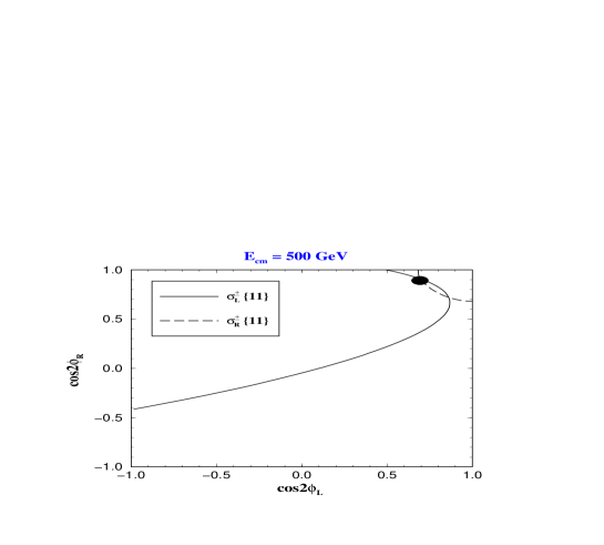
Figure 5: Contours of the chargino production cross–sections $\sigma^{\pm}_{L}\{11\}=341.1$ fb and $\sigma^{\pm}_{R}\{11\}=0.53$ fb for the light chargino mass $m_{\tilde{\chi}^{\pm}_{1}}=175.6$ GeV and the sneutrino mass $m_{\tilde{\nu}}=192.8$ GeV (the set ${\sf RP1}$) in the plane of $\{\cos 2\phi_{L},\,\cos 2\phi_{R}\}$ at the $e^{+}e^{-}$ c.m. energy of 500 GeV ; the two crossing points in the upper right corner are $\{0.699,\,0.906\}$ and $\{0.862,\,0.720\}$, respectively.

4.1 Light chargino and neutralino system

At the beginning of future $e^{+}e^{-}$ linear–collider operations, the energy may only be sufficient to reach the threshold of the light chargino pair $\tilde{\chi}^{+}_{1}\tilde{\chi}^{-}_{1}$ and of the neutralino pair $\tilde{\chi}^{0}_{1}\tilde{\chi}^{0}_{2}$. From the analysis of this restricted system, the entire structure of the gaugino/higgsino sector can be unraveled in CP–invariant theories on which we focus first for the sake of simplicity. As shown in Ref. [15], the chargino sector can be reconstructed up to at most a two–fold discrete ambiguity. On the other hand, if the analysis of the chargino and the neutralino systems is combined, ten physical observables can be measured: three masses and seven polarized cross sections, among which two masses and four cross sections are accessible in the neutralino system.

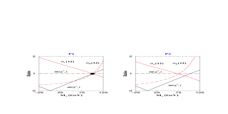
Figure 6: Ratios of $m_{\tilde{\chi}^{0}_{1}}$, $m_{\tilde{\chi}^{0}_{2}}$, $\sigma_{L}\{12\}$ and $\sigma_{R}\{12\}$ with respect to their measured values plotted as functions of $M_{1}$ for two possible solutions ${\sf P1}$ (left) and ${\sf P2}$ (right) derived from the chargino sector. The left panel gives a unique value $M_{1}=100.5$ GeV for the U(1) gaugino mass resolving the ${\sf P1}$–${\sf P2}$ ambiguity.

By analyzing the $\{11\}$ mode in $\sigma^{\pm}_{L}\{11\}$ and $\sigma^{\pm}_{R}\{11\}$, the chargino mixing angles $\cos 2\phi_{L}$ and $\cos 2\phi_{R}$ can be determined up to at most a four–fold ambiguity if the sneutrino mass is known and the SUSY Yukawa coupling is identified with the gauge coupling. The ambiguity can be resolved [15] by measuring the transverse cross–section $\sigma^{\pm}_{T}\{11\}$. On the other hand, initial beam polarization in the process $e^{+}e^{-}\rightarrow\tilde{\chi}^{0}_{1}\,\tilde{\chi}^{0}_{2}$ allows us to measure the two independent additional observables $\sigma_{R}\{12\}$ and $\sigma_{L}\{12\}$ in the neutralino system. Moreover, the light neutralino masses can be measured with high precision.

For illustration, we assume that at the c.m. energy $E_{cm}=500$ GeV the light chargino mass and the polarized cross sections of the light chargino pair are measured with good precision to be $m_{\tilde{\chi}^{\pm}_{1}}=175.6\,{\rm GeV}$ and $\sigma^{\pm}_{L/R}\{11\}=341.1\,{\rm fb}/0.53\,{\rm fb}$ and the sneutrino mass $m_{\tilde{\nu}}=192.8$ GeV, corresponding to ${\sf RP1}$.

The two ellipses in Fig.5 for the measured polarized cross sections $\sigma^{\pm}_{L,R}\{11\}$, as functions of $\cos 2\phi_{L}$ and $\cos 2\phi_{R}$, cross at two points:

$$\{\cos 2\phi_{{}_{L}},\,\cos 2\phi_{{}_{R}}\}=\{0.699,\,0.906\}\ \ {\rm and}\ \ \{0.862,\,0.720\}$$ (131)

Following the analysis described in Ref. [15], the cosines of the two mixing angles in eq. (131) and the light chargino mass $m_{\tilde{\chi}^{\pm}_{1}}=175.6$ GeV are sufficient to solve for the fundamental parameters $\{\tan\beta,\,M_{2},\,\mu\}$:

$$\begin{array}[]{llcl}{\sf P1}\,:&\{0.699,\,0.906\}&\Rightarrow&\{\tan\beta=\ \ 10;\,M_{2}=190.8\,{\rm GeV},\,\mu=365.1\,{\rm GeV}\}\\[5.69054pt] {\sf P2}\,:&\{0.862,\,0.720\}&\Rightarrow&\{\tan\beta=0.35;\,M_{2}=197.9\,{\rm GeV},\,\mu=387.7\,{\rm GeV}\}\end{array}$$ (134)

The ambiguity can be resolved in several ways: internally within the chargino sector by measuring the transverse cross–section $\sigma^{\pm}_{T}\{11\}$; externally by confronting the ensuing Higgs boson mass $m_{h^{0}}$ with the experimental value. However, the ambiguity can also be resolved by analyzing the $\tilde{\chi}^{0}_{1}\,\tilde{\chi}^{0}_{2}$ system for left and right polarized beams; at the same time the U(1) gaugino mass parameter can be determined unambiguously.

We assume the measured light neutralino and selectron masses to be those in eqs. (128) and (130) and the measured polarized cross sections $\sigma_{L,R}\{12\}$ to be 233.4 fb /22.1 fb, respectively, as predicted in ${\sf RP1}$. The expected values of $m_{\tilde{\chi}^{0}_{1}}$, $m_{\tilde{\chi}^{0}_{2}}$, $\sigma_{L}\{12\}$ and $\sigma_{R}\{12\}$ for the two possible solutions of eq. (134) can be calculated as functions of $M_{1}$ and compared with measured values. In Fig. 6 the ratios of the theoretically predicted values $m_{\tilde{\chi}^{0}_{1}}$, $m_{\tilde{\chi}^{0}_{2}}$, $\sigma_{L}\{12\}$ and $\sigma_{R}\{12\}$ for a given value of the mass parameter $M_{1}$ are displayed with respect to their measured values:

$${\rm Ratio}=m^{th}_{\tilde{\chi}^{0}_{i}}(M_{1})/m^{meas}_{\tilde{\chi}^{0}_{i}}\qquad{\rm and}\qquad\sigma^{th}(M_{1})/\sigma^{meas}$$ (135)

In the left panel the curves all meet in exactly one point proving that

$${\sf P1}:\qquad M_{1}=100.5\,{\rm GeV}$$ (136)

is the correct solution. Additional consistency checks can be provided by measuring the production cross sections $\sigma_{T}\{12\}$, if transversely polarized electron and positron beams are available.

4.2 The supersymmetric Yukawa couplings

The identity of the SUSY Yukawa couplings $g_{{}_{\tilde{W}}}$ and $g_{{}_{\!\tilde{B}}}$ with the SU(2) and U(1) gauge couplings $g$ and $g^{\prime}$, which is of fundamental importance in supersymmetric theories, can be tested very accurately in neutralino pair–production. This analysis is one of the final targets of LC experiments which should provide a complete picture of the electroweak gaugino sector with resolution at least at the per-cent level.

We assume here that the SU(2) gaugino/higgsino parameters in the CP–invariant theory have been pre–determined in the chargino sector and the U(1) parameter $M_{1}$ has been extracted from the neutralino mass spectrum. The equality between the Yukawa and the gauge couplings can be tested precisely by making use of electron (and positron) beam polarization. Varying the left–handed and right–handed Yukawa couplings leads to a significant change in the corresponding left–handed

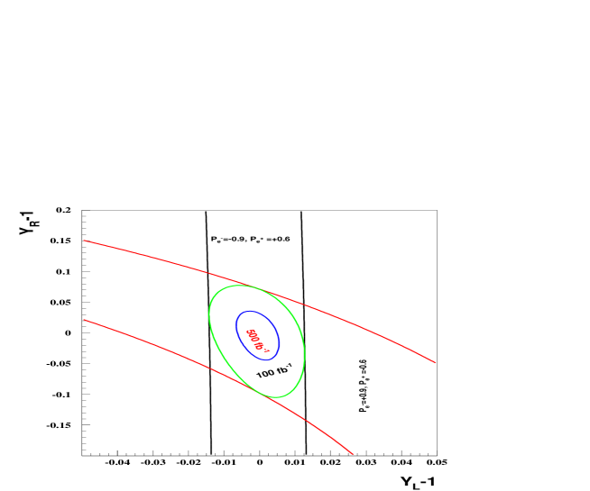
Figure 7: Contours of the cross sections $\sigma_{L}\{12\}$ and $\sigma_{R}\{12\}$ in the plane of the Yukawa couplings $g_{{}_{\tilde{W}}}$ and $g_{{}_{\!\tilde{B}}}$ normalized to the SU(2) and U(1) gauge couplings $g$ and $g^{\prime}$ $\{Y_{L}=g_{{\tilde{W}}}/g,\,Y_{R}=g_{{\tilde{B}}}/g^{\prime}\,\}$ for the set ${\sf RP1}$ at the $e^{+}e^{-}$ c.m. energy of 500 GeV; the contours correspond to the integrated luminosities 100 and 500 fb^-1 and the longitudinal polarization of electron and positron beams of 90% and 60%, respectively.

and right–handed production cross sections. Combining the measurements of $\sigma_{R}$ and $\sigma_{L}$ for the process $e^{+}e^{-}\rightarrow\tilde{\chi}^{0}_{1}\,\tilde{\chi}^{0}_{2}$ process, the Yukawa couplings $g_{{}_{\tilde{W}}}$ and $g_{{}_{\!\tilde{B}}}$ can be determined to quite a high precision as demonstrated in Fig. 7. The $1\sigma$ statistical errors have been derived for an integrated luminosity of $\int{\cal L}\,dt=100$ and $500$ fb^-1 and for partially polarized beams.

Combined with the measurement of the $\tilde{W}e\tilde{\nu}$ Yukawa coupling, including the analysis of angular distributions, in the chargino sector, it is possible to check the crucial SUSY relation between the gauge couplings and the supersymmetric Yukawa couplings in a comprehensive way.

4.3 The complete MSSM neutralino system

The measurements of the chargino–pair production processes $e^{+}e^{-}\rightarrow\tilde{\chi}^{+}_{i}\tilde{\chi}^{-}_{j}$ ($i,j$=1,2) carried out with polarized beams can be used for a complete determination of the basic SUSY parameters $\{M_{2},\,|\mu|,\,\Phi_{\mu}\,;\tan\beta\}$ in the chargino sector with high precision. In this section, it will be demonstrated analytically in the general CP–noninvariant theory that the real and imaginary parts of the U(1) gaugino mass $M_{1}$ can be determined subsequently from the measurements of (i) either three neutralino masses or/and (ii) from the masses of two light neutralinos and one neutralino–pair production cross section such as $\sigma\{12\}$.

Each of the four invariants $a$, $b$, $c$, $d$ of the matrix ${\cal M}{\cal M}^{\dagger}$, defined in eq. (64), is a second–order polynomial of $\Re{\rm e}{M_{1}}=|M_{1}|\,\cos\Phi_{1}$ and $\Im{\rm m}{M_{1}}=|M_{1}|\,\sin\Phi_{1}$. Therefore, each of the characteristic equations in the set (63) for the neutralino mass squared can be cast into the form

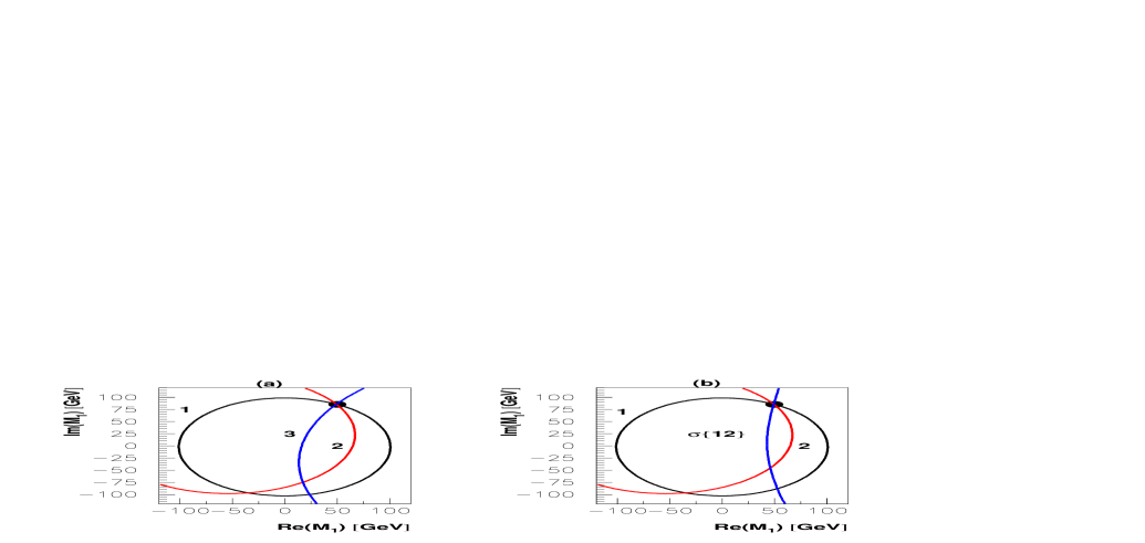
Figure 8: The contours of (a) three measured neutralino masses $m_{\tilde{\chi}^{0}_{i}}$ ($i=1,2,3$), and (b) two neutralino masses (1,2) and one neutralino production cross section $\sigma_{tot}\{12\}$ in the $\{\Re{\rm e}{M_{1}},\,\Im{\rm m}{M_{1}}\}$ plane; the parameter set ${\sf RP1^{\prime\prime}}$ $\{\tan\beta=10,\,M_{2}=190.8\,{\rm GeV},\,|\mu|=365.1\,{\rm GeV},\,\Phi_{\mu}=\pi/4\}$ is taken from the chargino sector.

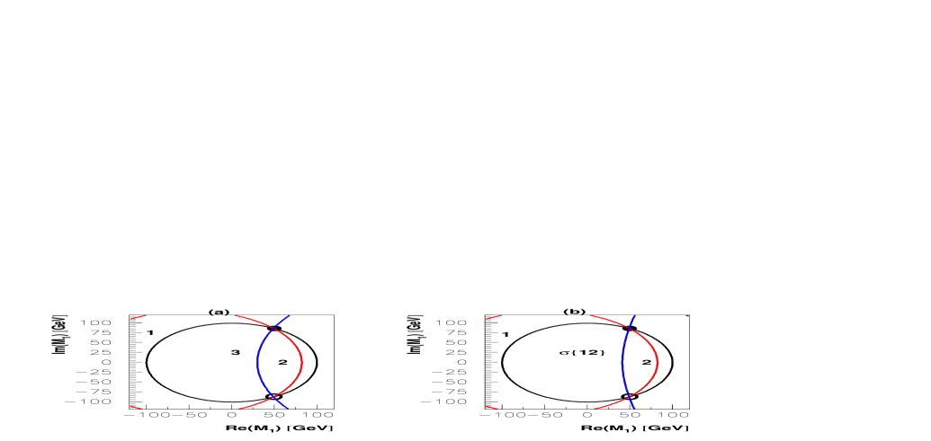
Figure 9: The contours of (a) three measured neutralino masses and (b) two measured light neutralino masses and one neutralino production cross section, $\sigma_{tot}\{12\}$ in the $\{\Re{\rm e}{M_{1}},\,\Im{\rm m}{M_{1}}\}$ plane for the CP–violating case ${\sf RP1^{\prime}}$: $\{\tan\beta=10,\,M_{2}=190.8\,{\rm GeV},\mu=365.1\,{\rm GeV},\,\sin\Phi_{\mu}=0\}$.

$$(\Re{\rm e}{M_{1}})^{2}+(\Im{\rm m}{M_{1}})^{2}+u_{i}\Re{\rm e}{M_{1}}+v_{i}\Im{\rm m}{M_{1}}=w_{i}\qquad(i=1,2,3,4)$$ (137)

The coefficients $u_{i}$, $v_{i}$ and $w_{i}$ are functions of the parameters $\tan\beta$, $M_{2}$, $|\mu|$, $\Phi_{\mu}$ pre–determined in the chargino sector, and the mass $m^{2}_{\tilde{\chi}^{0}_{i}}$; the coefficient $v_{i}$ is necessarily proportional to $\sin\Phi_{\mu}$ because physical masses are CP–even. For each neutralino mass, eq. (137) defines a circle in the $\{\Re{\rm e}{M_{1}},\Im{\rm m}{M_{1}}\}$ plane. As a result, the measurement of three neutralino masses leads to an unambiguous determination of the modulus and the phase of $M_{1}$, cf. Fig. 8(a). With only two light neutralino masses, the two–fold ambiguity can be resolved by exploiting the measured cross section $\sigma\{12\}$, as shown in Fig. 8(b). However, if the phase $\sin\Phi_{\mu}$ vanishes, there remains a two–fold discrete sign ambiguity in $\Im{\rm m}{M_{1}}$, as demonstrated in Fig.9.

5 Closure of the neutralino system

Since the reconstruction of the mass and mixing parameters is easy if all four neutralino states are detected, stringent tests of the four–state closure can be designed. Models with additional chiral or vector superfields, for example, give rise to extensions of the neutralino sector in general.

The four–state mixing of neutralinos in the minimal supersymmetric extension of the Standard Model induces sum rules for the neutralino couplings. They can be formulated in terms of the squares of the bilinear charges, i.e. the factorized elements of the quartic charges. This follows from the unitarity of the diagonalization matrices. If all possible neutralino states are summed up, the following general sum rules can be derived at tree level:

$$\sum_{i,j=1}^{4}\,{\cal Z}_{ij}{\cal Z}^{*}_{ij}=\frac{1}{2}\hskip 56.9055pt\sum_{i,j=1}^{4}\,g_{Lij}g^{*}_{Lij}=\frac{1}{16c^{4}_{W}s^{4}_{W}}$$

$$\sum_{i,j=1}^{4}\,{\cal Z}_{ij}g^{*}_{Lij}=0\hskip 56.9055pt\sum_{i,j=1}^{4}\,g_{Lij}g^{*}_{Rij}=\frac{1}{4c^{4}_{W}}$$

$$\sum_{i,j=1}^{4}\,{\cal Z}_{ij}g^{*}_{Rij}=0\hskip 56.9055pt\sum_{i,j=1}^{4}\,g_{Rij}g^{*}_{Rij}=\frac{1}{c^{4}_{W}}$$ (138)

The right–hand side of the sum rules is independent of the parameters in the neutralino system and it is given solely by the gauge group. Therefore, evaluating these sum rules experimentally, it can be tested whether the four–neutralino system $\{\tilde{\chi}_{1}^{0},\tilde{\chi}_{2}^{0},\tilde{\chi}_{3}^{0},\tilde{\chi}_{4}^{0}\}$ forms a closed system, or whether additional states at high mass scales mix in, signaling the existence of an extended gaugino system.

The validity of the sum rules is reflected in both the quartic charges and the production cross sections. However, due to mass effects and the $t$– and $u$–channel selectron exchanges, it is not straightforward to derive the sum rules for the quartic charges and the production cross sections in practice. Asymptotically at high energies, however, the sum rules in eq. (138) can be transformed directly into sum rules for the associated cross sections:

$$\lim_{s\rightarrow\infty}\,s\,\sum_{i\leq j}^{4}\,\sigma\{ij\}=\frac{\pi\alpha^{2}}{48\,c^{4}_{W}s^{4}_{W}}\left[64s^{4}_{W}-8s^{2}_{W}+5\right]$$ (139)

The approach to the asymptotic form of the sum rules depends on the mass parameters of the theory. (The mixing parameters, weighted by the physical neutralino masses, can be summed up to polynomials of the gaugino and higgsino mass parameters, as demonstrated in the appendix.)

In Fig. 10 the exact values for the summed-up cross sections normalized to the asymptotic value are shown for the reference point ${\sf RP1}$. The final state $\tilde{\chi}^{0}_{1}\tilde{\chi}^{0}_{1}$ is invisible in $R$-parity invariant theories, and its detection is difficult. Nevertheless, it can be studied directly by photon tagging in the final state $\gamma\tilde{\chi}^{0}_{1}\tilde{\chi}^{0}_{1}$, which can be observed at the LC. Indirectly the $\tilde{\chi}^{0}_{1}\tilde{\chi}^{0}_{1}$ cross section can be predicted by extracting, hypothetically, the MSSM parameters from the observed cross sections. The subsequent failure of saturating the sum rules would then be sufficient to conclude that the neutralino system of the MSSM is not closed indeed and additional states mix in.

Figure 10: The energy dependence of the sum of all the neutralino–pair production cross sections normalized to the asymptotic form of the summed up cross section; the solid line represents the exact sum in the MSSM; the dashed line the sum of the cross sections for the first four neutralino states in a specific parameter set of the (M+1)SSM.

More specifically, extended SUSY models with $n$ SU(2) doublet and $m$ SU(2) singlet chiral superfields may be considered in general. In these extended models, diagonalization of the mass matrix leads to $(2+2n+m)$ neutralino mass eigenstates. The fermion (higgsino) components of the chiral fields do not modify the structure of the $\tilde{\chi}^{0}_{i}e\tilde{e}_{L,R}$ vertices. While the higgsino singlets do not change the structure of the $Z$–neutralino–neutralino vertices, the neutral component of each additional higgsino doublet with hypercharge $\pm 1/2$ couples to the $Z$ boson exactly in the same way as $\tilde{H}^{0}_{1,2}$. So, the $Z$–neutralino–neutralino couplings are modified to read

$$\langle\tilde{\chi}^{0}_{iL}\,|Z|\tilde{\chi}^{0}_{jL}\rangle=-\frac{g}{2\,c_{W}}\sum_{a=1}^{n}\left[N_{i(1+2a)}N^{*}_{j(1+2a)}-N_{i(2+2a)}N^{*}_{j(2+2a)}\right]$$

$$\langle\tilde{\chi}^{0}_{iR}\,|Z|\tilde{\chi}^{0}_{jR}\rangle=+\frac{g}{2\,c_{W}}\sum_{a=1}^{n}\left[N^{*}_{i(1+2a)}N_{j(1+2a)}-N^{*}_{i(2+2a)}N_{j(2+2a)}\right]$$ (140)

The sum rule, following from the unitarity of the $(2+2n+m)\times(2+2n+m)$ mixing matrix, for the pair–production cross sections of all states is extended to

$$\lim_{s\rightarrow\infty}\,s\,\sum_{i\leq j}^{2+2n+m}\,\sigma\{ij\}=\frac{\pi\alpha^{2}}{48\,c^{4}_{W}s^{4}_{W}}\left[\,2\,(8s^{4}_{W}-4s^{2}_{W}+1)\,n+48s^{4}_{W}+3\right]$$ (141)

The right–hand side of eq. (141) is independent of the number $m$ of higgsino singlets and it reduces to the sum rule in the MSSM for $n=1$.

A typical example is provided by the extended (M+1)SSM scenario which incorporates an additional gauge singlet superfield [29], but does not change the structure of the charged sector. The superpotential of the (M+1)SSM is given by

$$W_{(M+1)SSM}=W_{Y}+\lambda\,SH_{1}H_{2}+\frac{1}{3}\kappa S^{3}$$ (142)

where $W_{Y}$ accounts for the lepton and quark Yukawa interactions. In this model, an effective $\mu=\lambda s$ term is generated when the scalar component of the singlet $S$ acquires a vacuum expectation value $s=\langle S\rangle$. The fermion component of the singlet superfield (singlino) will mix with neutral gauginos and higgsinos after electroweak gauge symmetry breaking, changing the neutralino mass matrix to the 5$\times$5 form

$${\cal M}_{(M+1)SSM}=\left(\begin{array}[]{ccccc}|M_{1}|\,{\rm e}^{i\Phi_{1}}&0&-m_{Z}c_{\beta}s_{W}&m_{Z}s_{\beta}s_{W}&0\\[5.69054pt] 0&M_{2}&m_{Z}c_{\beta}c_{W}&-m_{Z}s_{\beta}c_{W}&0\\[5.69054pt] -m_{Z}c_{\beta}s_{W}&m_{Z}c_{\beta}c_{W}&0&-|\mu|\,{\rm e}^{i\Phi_{\mu}}&-|M_{\lambda}|\,s_{\beta}\,{\rm e}^{i\Phi_{\lambda}}\\[5.69054pt] m_{Z}s_{\beta}s_{W}&-m_{Z}s_{\beta}c_{W}&-|\mu|\,{\rm e}^{i\Phi_{\mu}}&0&-|M_{\lambda}|\,c_{\beta}\,{\rm e}^{i\Phi_{\lambda}}\\[5.69054pt] 0&0&-|M_{\lambda}|\,s_{\beta}\,{\rm e}^{i\Phi_{\lambda}}&-|M_{\lambda}|\,c_{\beta}\,{\rm e}^{i\Phi_{\lambda}}&\,2|M_{\kappa}|\,{\rm e}^{i\Phi_{\kappa}}\end{array}\right)\$$

where $|M_{\lambda}|\,{\rm e}^{i\Phi_{\lambda}}\equiv\lambda v$ and $|M_{\kappa}|\,{\rm e}^{i\Phi_{\kappa}}\equiv\kappa s$.

In some regions of the parameter space [30] the singlino may be the lightest supersymmetric particle, weakly mixing with other states. Then displaced vertices in the (M+1)SSM may be generated, which would signal the extension of the minimal model. If the spectrum of the four lighter neutralinos in the extended model is similar to the spectrum in the MSSM but the mixing is substantial, discriminating the models by analyzing the mass spectrum becomes very difficult. Studying in this case the summed-up cross sections of the four light neutralinos may then be a crucial method to reveal the structure of the neutralino system.

In Fig.10 the exact sum rules are also included for a possible scenario of the (M+1)SSM; the parameters $M_{1}=1000$ GeV, $M_{2}=169$ GeV, $\mu=-263$ GeV, $\tan\beta=10$ and $M_{\lambda}=263$ GeV, $M_{\kappa}=-59$ GeV, give rise to one very heavy neutralino with $m_{\tilde{\chi}^{0}_{5}}\sim 1000$ GeV, and to four lighter neutralinos with masses within 2 – 5 GeV equal to the neutralino masses for the ${\sf RP1}$ point of the MSSM. Due to the incompleteness of these states below the thresholds for producing the heavy neutralino, the (M+1)SSM value differs significantly from the corresponding sum rule of the MSSM. Therefore, even if the extended neutralino states are very heavy, the study of sum rules can shed light on the underlying structure of the supersymmetric model.

Addendum: Charginos
Asymptotically at high energies the sum rule

$$\lim_{s\rightarrow\infty}\,s\,\sum_{ij}^{2}\,\sigma^{\pm}\{ij\}=\frac{\pi\alpha^{2}}{24\,c^{4}_{W}s^{4}_{W}}\left[8s^{4}_{W}-8s^{2}_{W}+5\right]$$ (144)

for the summed-up chargino cross sections [15] can be derived in the same way. In analogy to the neutralino system, the approach to asymptotia depends on the gaugino and higgsino parameters, cf. appendix.

6 Conclusions

In the first part of this analysis we have derived the mass eigenvalues and the mixing matrix of the MSSM neutralino system including CP violation. The problem has been solved analytically, and a compact representation has been found in the limit of large SUSY gaugino and higgsino mass parameters compared to the scale of electroweak symmetry breaking. Unitarity quadrangles have been introduced, distinctly different from CKM and MNS polygons due to the Majorana nature of the neutralinos. They illustrate nicely the specific realization of CP violation through the two distinct sets of phases in the system. In this way the solution of the MSSM neutralino system has been advanced to a level analogous to the chargino system.

If the chargino system is solved for the SU(2) parameters $\{M_{2},|\mu|,\Phi_{\mu};\tan\beta\}$, the neutralino mass spectrum is sufficient to extract the U(1) gaugino mass parameter $\{|M_{1}|,\Phi_{1}\}$. Three (light) neutralino masses $m_{\tilde{\chi}^{0}_{1,2,3}}$ or/and two light neutralino masses $m_{\tilde{\chi}^{0}_{1,2}}$ supplemented by the production cross section $\sigma\{12\}$ for the neutralino pair $\tilde{\chi}^{0}_{1}\tilde{\chi}^{0}_{2}$, allow us to extract $\{|M_{1}|,\Phi_{1}\}$ unambiguously, and with a two–fold ambiguity for the sign of $\sin\Phi_{1}$ if $\sin\Phi_{\mu}$ vanishes. This discrete ambiguity can be solved by measuring the normal neutralino polarization and/or the cross section $\sigma_{N}$ with initial transverse beam polarization. All fundamental SU(2)$\times$U(1) gaugino and higgsino parameters can therefore be derived analytically in the combined chargino $\oplus$ neutralino system from measured mass and mixing parameters.

Sum rules for the production cross sections can be used at high energies to probe whether the four–state neutralino system is closed or whether additional states mix in from potentially very high scales.

To summarize. The measurement of the processes $e^{+}e^{-}\rightarrow\tilde{\chi}^{0}_{i}\tilde{\chi}^{0}_{j}$ ($i,j$=1,2,3,4), carried out with polarized beams and combined with the analysis of the chargino system $e^{+}e^{-}\rightarrow\tilde{\chi}^{+}_{i}\tilde{\chi}^{-}_{j}$ ($i,j$=1,2), can be used to perform a complete and precise analysis of the basic SUSY parameters in the gaugino/higgsino sector $\{M_{1},M_{2},\mu;\tan\beta\}$. The chargino/neutralino system of the MSSM at tree level is therefore under analytical control in toto.

Since the analysis can be performed with high precision, this set provides a solid platform for extrapolations to scales eventually near the Planck scale where the fundamental supersymmetric theory may be defined.

APPENDIX

Appendix A Sum Rules: Approach to Asymptotia

While the sum rules in the asymptotic limit do not depend on any supersymmetry parameters of the gaugino/higgsino sector but only on the gauge group, the approach to asymptotia involves the neutralino and chargino masses. Nevertheless, the sums of the mixing parameters weighted by these masses, can be expressed by the fundamental gaugino and higgsino mass parameters in closed form.

A.1 Neutralino system

The following mass weighted sum rules

$$\sum^{4}_{ij}m^{2}_{i}|{\cal Z}_{ij}|^{2}=\frac{m_{Z}^{2}+2|\mu|^{2}}{4}\qquad\hskip 28.45274pt\sum^{4}_{ij}m_{i}m_{j}|{\cal Z}_{ij}|^{2}=-\frac{|\mu|^{2}}{2}$$

$$\sum^{4}_{ij}m^{2}_{i}|g_{Rij}|^{2}=\frac{|M_{1}|^{2}+m^{2}_{Z}s^{2}_{W}}{c^{4}_{W}}\quad\hskip 19.91684pt\sum^{4}_{ij}m^{2}_{i}|g_{Lij}|^{2}=\frac{|M_{1}|^{2}s^{2}_{W}+|M_{2}|^{2}c^{2}_{W}+m^{2}_{Z}c^{2}_{2W}}{16\,c^{4}_{W}s^{4}_{W}}$$

$$\sum^{4}_{ij}m_{i}m_{j}g_{Rij}^{2}=\frac{|M_{1}|^{2}}{c^{4}_{W}}\ \ \hskip 69.70915pt\sum^{4}_{ij}m_{i}m_{j}g_{Lij}^{2}=\frac{|M_{1}s^{2}_{W}+M_{2}c^{2}_{W}|^{2}}{16c^{4}_{W}s^{4}_{W}}$$

$$\sum^{4}_{ij}m_{i}m_{i}{\cal Z}_{ij}g_{Rij}=\frac{m^{2}_{Z}s^{2}_{W}\,c_{2\beta}}{2c^{2}_{W}}\qquad\hskip 17.92537pt\sum^{4}_{ij}m_{i}m_{i}{\cal Z}_{ij}g_{Lij}=\frac{m^{2}_{Z}\,c^{2}_{2W}c_{2\beta}}{8c^{2}_{W}s^{2}_{W}}$$ (145)

and

$$\sum^{4}_{ij}m^{2}_{i}m^{2}_{j}|g_{Lij}|^{2}\!\! = \left[|M_{1}|^{2}s^{2}_{W}+|M_{2}|^{2}c^{2}_{W}+m^{2}_{Z}c^{2}_{2W}\right]^{2}/16\,c^{4}_{W}s^{4}_{W}$$

$$\sum^{4}_{ij}m^{2}_{i}m^{2}_{j}|g_{Rij}|^{2}\!\! = \left[|M_{1}|^{2}+m^{2}_{Z}s^{2}_{W}\right]^{2}/c^{4}_{W}$$ (146)

can be used in the sum of the neutralino cross sections

$$\lim_{s\rightarrow\infty}\,s\,\sum_{i\leq j}^{4}\,\sigma\{ij\}=\frac{\pi\alpha^{2}}{48\,c^{4}_{W}s^{4}_{W}}\left\{\,[\,64s^{4}_{W}-8s^{2}_{W}+5\,]\,+\Delta^{0}_{1}/s+\Delta^{0}_{2}/s\right\}$$ (147)

to calculate the coefficients $\Delta^{0}_{1}$ and $\Delta^{0}_{2}$ which control the approach to asymptotia:

$$\Delta^{0}_{1} = (8s^{4}_{W}-4s^{2}_{W}+1)m^{2}_{Z}+3m^{2}_{\tilde{e}_{L}}+48s^{4}_{W}m^{2}_{\tilde{e}_{R}}$$

$$-192s^{4}_{W}(|M_{1}|^{2}+m^{2}_{Z}s^{2}_{W})-12(|M_{1}|^{2}s^{2}_{W}+|M_{2}|^{2}c^{2}_{W}+m^{2}_{Z}c^{2}_{2W})$$

$$+6\left\{|M_{1}-M_{2}|^{2}s^{2}_{2W}/4+m^{2}_{Z}c^{2}_{2W}(1+c_{2W}c_{2\beta})-m^{2}_{\tilde{e}_{L}}\right\}\log\left(1+s/m^{2}_{\tilde{e}_{L}}\right)$$

$$+48s^{4}_{W}\left\{m^{2}_{Z}s^{2}_{W}(2+c_{2\beta})-2m^{2}_{\tilde{e}_{R}}\right\}\log\left(1+s/m^{2}_{\tilde{e}_{R}}\right)$$

$$\Delta^{0}_{2} = \frac{3}{m^{2}_{\tilde{e}_{L}}}\left\{|M_{1}|^{2}s^{2}_{W}+|M_{2}|^{2}c^{2}_{W}+m^{2}_{Z}c^{2}_{2W}\right\}^{2}+\frac{48s^{4}_{W}}{m^{2}_{\tilde{e}_{R}}}\left\{|M_{1}|^{2}+m^{2}_{Z}s^{2}_{W}\right\}^{2}$$ (148)

The approach to asymptotia is fast for the reference point chosen before. For $\sqrt{s}=2$ TeV the form including the subleading terms in eqs. (147) and (148) has reached already 90 percent of the asymptotic limit.

A.2 Chargino system

The coefficients $\Delta^{\pm}_{1,2}$ in the sum rule for the chargino cross sections

$$\lim_{s\rightarrow\infty}\,s\,\sum_{ij}^{2}\,\sigma^{\pm}\{ij\}=\frac{\pi\alpha^{2}}{24\,c^{4}_{W}s^{4}_{W}}\left\{\,[\,8s^{4}_{W}-8s^{2}_{W}+5\,]\,+\Delta^{\pm}_{1}/s+\Delta^{\pm}_{2}/s\right\}$$ (149)

can be evaluated in the same way:

$$\Delta^{\pm}_{1} = 2(6s^{6}_{W}+5s^{4}_{W}-8s^{2}_{W}+2)\,m^{2}_{Z}-3(8s^{4}_{W}-4s^{2}_{W}+1)\,m^{2}_{W}$$

$$+18\,c^{4}_{W}m^{2}_{\tilde{\nu}}-24c^{4}_{W}(|M_{2}|^{2}+2m^{2}_{W}c^{2}_{\beta})$$

$$-12c^{2}_{W}\left[m^{2}_{\tilde{\nu}}\,c^{2}_{W}+m^{2}_{W}c^{2}_{\beta}(2s^{2}_{W}-1)\right]\log\left(1+s/m^{2}_{\tilde{\nu}}\right)$$

$$\Delta^{\pm}_{2} = \frac{6}{m^{2}_{\tilde{\nu}}}\,c^{4}_{W}(|M_{2}|^{2}+2m^{2}_{W}c^{2}_{\beta})^{2}$$ (150)

Again, the approach to asymptotia is fast for the parameter set under discussion.

Acknowledgments

SYC was supported by the Korea Research Foundation Grant (KRF–2000–015–DS0009), JK by the KBN Grant No. 2P03B 060 18. The work was supported in part by the European Commission 5-th Framework Contract HPRN-CT-2000-00149. SYC and JK acknowledge the hospitality extended to them at DESY by Profs. Klanner and Wagner. We also thank H. Fraas, H. Haber, T. Han, W. Hollik, J.-L. Kneur, U. Martyn and G. Moultaka for useful discussions.

References

- [1] For reviews, see H. Nilles, Phys. Rep. 110 (1984) 1; H. E. Haber and G. L. Kane, Phys. Rep. 117 (1985) 75.
- [2] Y. Kizukuri and N. Oshimo, Phys. Lett. B 249 (1990) 449; T. Ibrahim and P. Nath, Phys. Rev. D 58 (1998) 111301 [Erratum-ibid. D 60 (1998) 099902] [hep-ph/9807501] and hep–ph/0107325; T. Ibrahim and P. Nath, Phys. Rev. D 61, 093004 (2000) [hep-ph/9910553]; M. Brhlik, G.J. Good and G.L. Kane, Phys. Rev. D 59 (1999) 115004; R. Arnowitt, B. Dutta and Y. Santoso, hep-ph/0106089;
- [3] V. Barger, T. Falk, T. Han, J. Jiang, T. Li and T. Plehn, hep-ph/0101106.
- [4] J. Ellis, J. M. Frère, J. S. Hagelin, G. L. Kane and S. T. Petcov, Phys. Lett. B 132 (1983) 436.
- [5] A. Bartl, H. Fraas and W. Majerotto, Nucl. Phys. B 278 (1986) 1.
- [6] T. Tsukamoto, K. Fujii, H. Murayama, M. Yamaguchi and Y. Okada, Phys. Rev. D 51 (1995) 3153; J. L. Feng, M. E. Peskin, H. Murayama and X. Tata, Phys. Rev. D 52 (1995) 1418.
- [7] E. Accomando et al. [ECFA/DESY LC Physics Working Group], Phys. Rep. 299 (1998) 1 [hep-ph/9705442].
- [8] TESLA Technical Design Report, Part: III Physics at an Linear Collider, eds. R.-D. Heuer, D. Miller, F. Richard and P. Zerwas, DESY 2001-011, ECFA 2001-209 [hep-ph/0106315].
- [9] G. Moortgat-Pick and H. Fraas, Phys. Rev. D 59 (1999) 015016 [hep-ph/9708481]; G. Moortgat-Pick, H. Fraas, A. Bartl and W. Majerotto, Eur. Phys. J. C 9 (1999) 521 [Erratum-ibid. C 9 (1999) 549] [hep-ph/9903220].
- [10] G. Moortgat-Pick, A. Bartl, H. Fraas and W. Majerotto, Eur. Phys. J. C 18 (2000) 379 [hep-ph/0007222].
- [11] S. Y. Choi, H. S. Song and W. Y. Song, Phys. Rev. D 61 (2000) 075004 [hep-ph/9907474].
- [12] G. Moortgat-Pick and H. Fraas, hep–ph/0012229.
- [13] J. L. Kneur and G. Moultaka, Phys. Rev. D 59 (1999) 015005 [hep-ph/9807336]; V. Barger, T. Han, T. Li and T. Plehn, Phys. Lett. B 475 (2000) 342 [hep-ph/9907425]; J. L. Kneur and G. Moultaka, Phys. Rev. D 61 (2000) 095003 [hep-ph/9907360].
- [14] S. Y. Choi, A. Djouadi, H. Dreiner, J. Kalinowski and P. M. Zerwas, Eur. Phys. J. C 7 (1999) 123 [hep-ph/9806279].
- [15] S. Y. Choi, M. Guchait, J. Kalinowski and P. M. Zerwas, Phys. Lett. B 479 (2000) 235 [hep-ph/0001175]; S. Y. Choi, A. Djouadi, M. Guchait, J. Kalinowski, H. S. Song and P. M. Zerwas, Eur. Phys. J. C 14 (2000) 535 [hep-ph/0002033].
- [16] S. Kiyoura, M. M. Nojiri, D. M. Pierce and Y. Yamada, Phys. Rev. D 58 (1998) 075002 [hep-ph/9803210]; T. Blank and W. Hollik, hep-ph/0011092; T. Blank, PhD Thesis, Karlsruhe 2000, http://www-itp.physik.uni-karlsruhe.de/prep/phd/; H. Eberl, M. Kincel, W. Majerotto and Y. Yamada, hep-ph/0104109.
- [17] G. A. Blair, W. Porod and P. M. Zerwas, Phys. Rev. D 63 (2001) 017703 [hep-ph/0007107].
- [18] L. Chau and W. Keung, Phys. Rev. Lett. 53 (1984) 1802; M. Gronau and J. Schechter, Phys. Rev. Lett. 54 (1985) 385 [Erratum-ibid. 54 (1985) 1209]; H. Fritzsch and J. Plankl, Phys. Rev. D 35 (1987) 1732.
- [19] C. Jarlskog, Phys. Rev. Lett. 55 (1985) 1039.
- [20] F. J. Botella and L. Chau, Phys. Lett. B 168 (1986) 97; J. D. Bjorken and I. Dunietz, Phys. Rev. D 36 (1987) 2109.
- [21] F. del Aguila and J. A. Aguilar-Saavedra, Phys. Lett. B 386 (1996) 241 [hep-ph/9605418]; J. A. Aguilar-Saavedra and G. C. Branco, Phys. Rev. D 62 (2000) 096009 [hep-ph/0007025].
- [22] A. Bartl, H. Fraas, W. Majerotto and N. Oshimo, Phys. Rev. D 40 (1989) 1594; M. M. El Kheishen, A. A. Aboshousha and A. A. Shafik, Phys. Rev. D 45 (1992) 4345; M. Guchait, Z. Phys. C 57 (1993) 157 [Erratum-ibid. C 61 (1993) 178]; G. J. Gounaris, C. Le Mouël and P. I. Porfyriadis, hep–ph/0107249.
- [23] J. N. Bronstein and V. A. Semendjajew, Taschenbuch der Mathematik, (Harri Deutsch, Frankfurt/M, 1961).
- [24] J. F. Gunion and H. E. Haber, Phys. Rev. D 37 (1988) 2515.
- [25] L. M. Sehgal and P .M. Zerwas, Nucl. Phys. B183 (1981) 417.
- [26] G. Weiglein et al., ”Higgs SUSY Working Group”, Snowmass 2001; A. Djouadi et al., Euro–Groupement der Recherche ”Supersymétrie”, Aix–la–Chapelle, Juin 2001; A. Djouadi et al., hep–ph/0107316; M. Battaglia et al., hep–ph/0106204.
- [27] H. Martyn and G. A. Blair, hep-ph/9910416.
- [28] S. Ambrosanio, B. Mele, G. Montagna, O. Nicrosini and F. Piccinini, Nucl. Phys. B 478 (1996) 46 [hep-ph/9601292].
- [29] J. Ellis, J. F. Gunion, H. E. Haber, L. Roszkowski and F. Zwirner, Phys. Rev. D 39 (1989) 844; U. Ellwanger and C. Hugonie, Eur. Phys. J. C 13 (2000) 681 [hep-ph/9812427]; F. Franke and H. Fraas, Z. Phys. C 72 (1996) 309 [hep-ph/9511275]; S. F. King and P. L. White, Phys. Rev. D 52, 4183 (1995) [hep-ph/9505326]; T. Elliott, S. F. King and P. L. White, Proceedings of the Workshop on Electroweak Symmetry Breaking, Budapest, 1994; R. B. Nevzorov, K. A. Ter–Martirosyan and M. A. Trusov, hep–ph/0105178.
- [30] S. Hesselbach, F. Franke and H. Fraas, Phys. Lett. B 492 (2000) 140 [hep-ph/0007310].