Chiral Lagrangians^∗ LU TP 01-26
hep-ph/0108111
August 2001

Abstract

An overview of the field of Chiral Lagrangians is given. This includes Chiral Perturbation Theory and resummations to extend it to higher energies, applications to the muon anomalous magnetic moment, $\epsilon^{\prime}/\epsilon$ and others.

1 Introduction

Chiral Symmetry is important in a lot of situations. In this talk I will restrict myself to consequences of Chiral Symmetry for the strong interaction. The subject is very broad as can be judged from the lectures and review articles[2]. In its modern form it was founded by Weinberg[6] and Gasser and Leutwyler.[7, 8] I will discuss a few of the basics in sects. 2, 3, 4. The applications to $\pi\pi$ scattering (sect. 5), some two-flavour results (sect. 6) and resummations, and the question of hadronic contributions to the muon magnetic moment (sect. 7), follow. Some of the theoretical developments in the structure and understanding in particular of the many free parameters follow in sect. 8. Applications to three flavours, sect. 9, quark mass ratios, sect. 10, $V_{us}$, sect. 11, anomalies and eta decays, sects. 12, 13, semileptonic, sect. 14, and nonleptonic, sect. 15 weak decays and $\epsilon^{\prime}/\epsilon$ form the main remaining part. I then conclude by a solar and cosmological as well as a high density application together with some references to neglected areas.

More than 300 papers cited one of the three seminal papers in the last two years, obviously necessitating many omissions.

2 Chiral Symmetry

QCD with 3 light quarks of equal mass has an obvious symmetry under continuous interchange of the quark flavours. This is the well known $SU(3)_{V}$. However, for $m_{q}=0$,

$${\cal L}_{QCD} = \sum_{q=u,d,s}\left[i\bar{q}_{L}D\hskip-6.45831pt/\,q_{L}+i\bar{q}_{R}D\hskip-6.45831pt/\,q_{R}\right.$$ (1)

$$\left.-m_{q}\left(\bar{q}_{R}q_{L}+\bar{q}_{L}q_{R}\right)\right]$$

has as symmetry the full chiral $SU(3)_{L}\times SU(3)_{R}$ since the left and right handed quarks decouple. Massive particles can always be changed from left to right handed by going to a Lorentzframe that moves faster than the particle, this changes the momentum direction but not the spin direction and hence flips the helicity. For massless particles this argument fails and the left and right helicities can thus be rotated separately.

Chiral Symmetry is broken by the vacuum of QCD, otherwise we would see a parity partner of the proton at a similar mass. Instead we believe that this symmetry is spontaneously broken by a quark-antiquark condensate or vacuum-expectation-value (VEV)

$$\langle\bar{q}q\rangle=\langle\bar{q}_{L}q_{R}+\bar{q}_{R}q_{L}\rangle\neq 0\,.$$ (2)

This condensate breaks $SU(3)_{L}\times SU(3)_{R}$ down to the diagonal subgroup $SU(3)_{V}$. This breaks 8 continuous symmetries and we must thus have 8 massless particles, Goldstone Bosons, whose interactions vanish at zero momentum.

The VEV that spontaneously breaks the Chiral Symmetry can also be a different one than in Eq. (2). This option is often known as Generalized Chiral Perturbation Theory.[9]

3 Uses of Chiral Symmetry

Chiral Symmetry can be used in high energy and nuclear physics in a variety of ways:

• Constructing chirally invariant phenomenological Lagrangians to be used only at tree level.

• Current Algebra which directly uses the Ward Identities of $SU(3)_{L}\times SU(3)_{R}$ and the Goldstone Boson nature of the pion to restrict amplitudes. Often these calculations assume smoothness assumptions on the amplitudes. This method is very powerful but becomes unwieldy when going beyond the leading terms.

• Chiral Perturbation Theory (CHPT) which is the modern implementation of current algebra using the full power of effective field theory (EFT) methods. In recent years CHPT methods have been developed for most areas where current algebra is applicable in particular for mesons with two and three flavours, single baryons, two or three baryons, and also in including nonleptonic weak and electromagnetic interactions.

• Using dispersion relations with CHPT constraints as a method to include higher orders and/or extend the range of validity of the CHPT results.

• The use of all the above in estimating weak nonleptonic decays and in particular $\epsilon^{\prime}/\epsilon$.

4 Chiral Perturbation Theory

As degrees of freedom we use the eight Goldstone Bosons of spontaneous chiral symmetry breaking, identified with the $\pi,K,\eta$ octet, and we expand in momenta using the fact that the interaction vanishes at zero momentum. The precise procedure can be found in many lectures[2] but is referred to as powercounting in generic momenta ($p$), external currents and quark masses. The usual ordering is $m_{q}\sim p^{2}$ since $m_{\pi}^{2}\sim p^{2}\sim m_{q}\langle\bar{q}q\rangle$ and we count external photon $Z^{0}$ and $W^{\pm}_{\mu}$ fields as order $p$ since they occur together with a momentum in the covariant derivative

$$D_{\mu}=\partial_{\mu}-ieA_{\mu}\,.$$ (3)

An example for the powercounting in $\pi\pi$-scattering is shown below:
0.5 Meson Vertex $p^{2}$
meson propagator $1/p^{2}$
$\int d^{4}p$ loop integral $p^{4}$
$(p^{2})^{2}\,(1/p^{2})^{2}\,p^{4}=p^{4}$
$(p^{2})\,(1/p^{2})\,p^{4}=p^{4}$
The lowest order diagram is just the tree level vertex at $p^{2}$ and as can be seen the two one-loop diagrams are both $p^{4}$. The existence of this loop expansion was shown in a very nice paper by Weinberg.[6] This paper can really be considered the birth of modern CHPT.

5 $\pi$-$\pi$ scattering

The amplitude for $\pi$-$\pi$ scattering can, in isospin notation, be written as

$$A(\pi^{i}\pi^{j}\to\pi^{k}\pi^{l})=i\delta^{ij}\delta^{kl}A(s,t,u)+\mbox{ cyclic}\,.$$

The fact that $\pi$-$\pi$ scattering is weak near threshold is one of the major qualitative predictions of spontaneous chiral symmetry breaking. The order $p^{2}$ contribution was worked out using current algebra methods by Weinberg in the sixties:[10]

$$A(s,t,u)=(s-m_{\pi}^{2})/F_{\pi}^{2}\,.$$ (4)

The $p^{4}$, including loop-diagrams and the new free parameters, was done by Gasser and Leutwyler[11] and the full two-loop expression was performed recently[12] after partial calculations in[13]. Remarkably the full amplitude can be written in terms of logarithms and other elementary functions.

The new results in the last year are that the Roy equation analysis was updated using the larger computer power now available[14] and the new data from the BNL-E865 experiment[15]. Both of these were then combined with the two-loop CHPT results in [16] with the conclusions that standard CHPT works find and that, at least in the two-flavour sector, the more generalized scenario (GCHPT) is not needed.

In Fig. 1 we show their conclusions

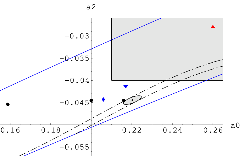
Figure 1: The conclusions of the new data on $\pi\pi$ scattering analyzed using CHPT and Roy equations. The triangle, $\blacktriangle$, and the shaded region are the old data. The band shows the Roy constraints and $\blacklozenge,\blacktriangledown$ are two predictions of pure CHPT indicating the uncertainty in the parameters. The dash-dotted band is the Roy equation analysis including (G)CHPT constraints and the ellipse shows the result of the new data. The bullets from left to right show the convergence of standard CHPT at orders $p^{2,4,6}$. From${}^{\ref{pipifinal}}$.

and in Fig. 2 the agreement with the old and the new data.

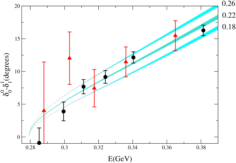
Figure 2: $\bullet$ are the new BNL E865 data and $\blacktriangle$ the older Rosselet${}^{\ref{Rosselet}}$ ones. The three bands are the predictions for three different values of the scattering length $a_{0}^{0}$. Figure from ${}^{\ref{pipifinal}}$.

In the future we expect a further improvement from measurements in $K_{e4}$ at KLOE and from pionium atoms at DIRAC.[18] The theoretical calculations needed for the latter data were recently completed.[19]

6 Other 2 flavour CHPT

The first two-loop calculation in CHPT was the two-flavour process $\gamma\gamma\to\pi^{0}\pi^{0}$ and its polarizabilities[20] and the equivalent calculation for the charged pions.[21] The latter also included the pion mass and decay-constants, see also.[12]

Radiative pion decay, $\pi\to\ell\nu\gamma$, is also known.[22] The most recent calculation in this sector was the full CHPT calculation of the pion scalar and vector form factors.[23] There has since been quite some work trying to add dispersion theoretical constraints to the pion vector form factor. Using inverse amplitude methods and Omnès equation inspired resummations a very nice fit to the ALEPH[26] and CLEO-II[27] data for $\tau$-decay was obtained. Similar work, with references to earlier work is [25].

In Fig. 3 I show the quality of the fit to the $\tau$-data. Good fits up to $\sqrt{s}\sim 1.5~{}GeV$ are obtained also for the $e^{+}e^{-}\to\pi^{+}\pi^{-}$ data and the spacelike $e\pi\to e\pi$ data[28] as shown in Fig. 4. The resummations in this sector work well, in Table 1 I show the charge radius and the coefficient of the quartic $q^{4}$ term in the vector form factor from the dispersive fit[24] and the pure CHPT fit.[23] Notice the quality of the agreement and the similarity of the errors even though the dispersive fit is dominated by the data around the rho peak and the CHPT fit by the spacelike data.

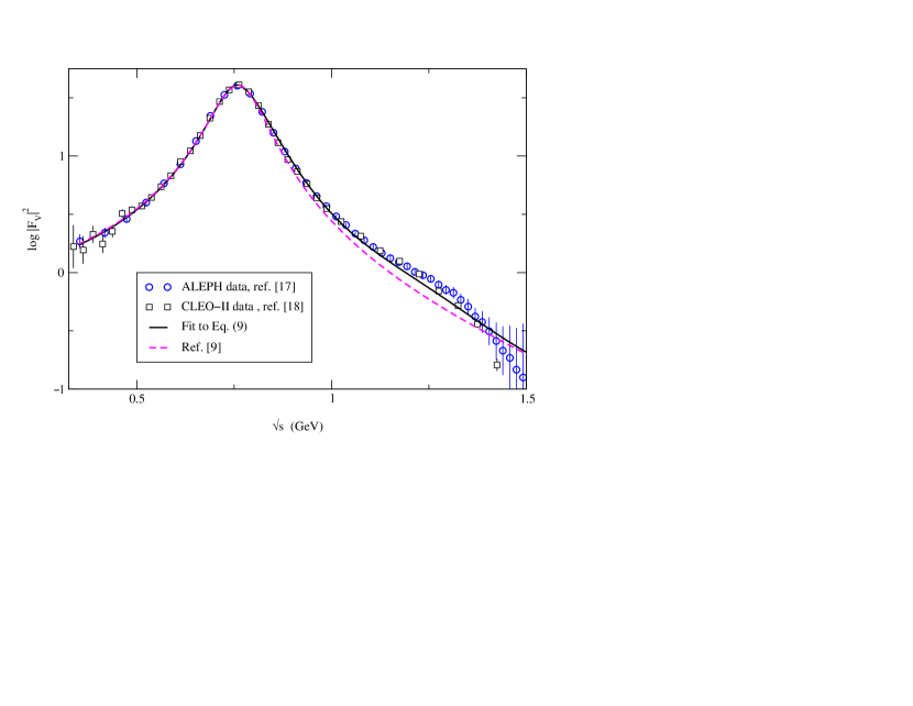
Figure 3: The resummed CHPT expression and the fit to the $\tau\to\pi\pi\nu$ data. Figure from ${}^{\ref{PichPortoles}}$.

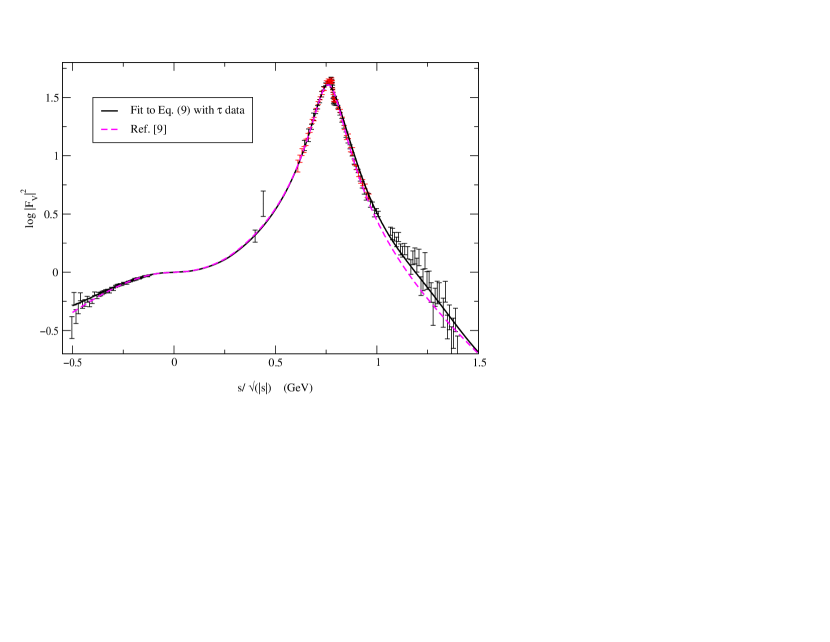
Figure 4: The resummed CHPT expression and the fit to the $e^{+}e^{-}$ and spacelike data. Figure from ${}^{\ref{PichPortoles}}$.

	dispersive	CHPT
$\langle r^{2}\rangle^{\pi}_{V}$ (GeV -2)	$11.04(30)$	$11.22(41)$
$c^{\pi}_{V}$ (GeV-4)	$3.79(4)$	$3.85(60)$

Table 1: Comparison between the CHPT fits and the dispersive improvement for the pion charge radius and the next term in formfactor expansion.

7 $a_{\mu}$: muon magnetic moment

The measurement[30] is

$$a_{\mu}=116~{}592~{}023(151)~{}\times~{}10^{-11}$$ (5)

while a recent theory review quotes the standard model prediction[31]

$$a_{\mu}=116~{}591~{}597(67)~{}\times~{}10^{-11}\,.$$ (6)

The difference is a few sigma depending on how errors are combined. The size of the theory error has been disputed by many people, varying from an “I don’t believe it” to more reasonable partial studies, an example of the latter is [32].

The methods of Chiral Lagrangians contribute to this theory prediction in various ways

1. The very low energy vacuum polarization contribution.

2. The effects of isospin breaking, in particular the issue of $\tau\to\pi\pi\nu$ data versus $e^{+}e^{-}\to\pi\pi$ data.

3. The calculation of the hadronic contribution to light-by-light scattering.

4. The  EFT calculation of higher order electroweak corrections.[33]

I now discuss the first three in more detail.

7.1 $a_{\mu}$: vacuum-polarization

The hadronic vacuum polarization contribution is depicted in Fig. 5.

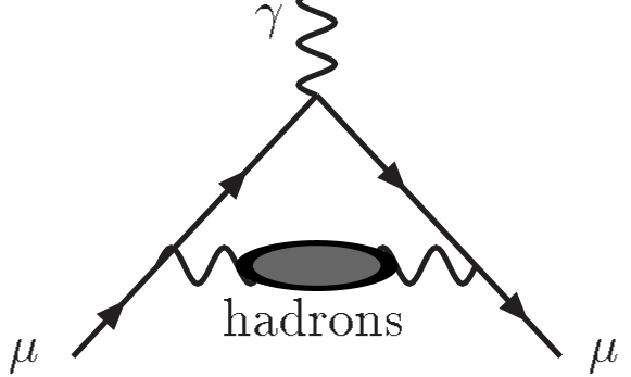
Figure 5: The hadronic vacuum polarization contribution to the muon anomalous magnetic moment.

The theory expression can be related to an integral over the experimentally observable ratio of hadronic events to $\mu^{+}\mu^{-}$ pairs in $e^{+}e^{-}$ collisions:

$$a_{\mu}=\left(\frac{\alpha m_{\mu}}{3\pi}\right)^{2}\int_{4m_{\pi}^{2}}^{\infty}dt\,R(t)\frac{\hat{K}(t)}{t^{2}}\,.$$ (7)

Here $\hat{K}(t)$ is a slowly varying function whose expression can be found in many places.[34] The contributions at low energies are enhanced but due to the very strong rho peak it is still dominated by that.

Pure CHPT methods can be used at $\sqrt{t}\leq 0.5$ GeV. Using the two-loop expression for the pion form factor with all available low-energy data yields[23]

$$10^{11}a_{\mu}^{\pi\pi}(\sqrt{t}\leq 0.5~{}GeV)=563\pm 30\,.$$ (8)

The error is mainly experimental, the best fit changes quite considerably depending on whether the timelike NA7 data[29] are included and the error on (8) reflects this.

The use of dispersion relations and resummations of the CHPT result[24] allows to go higher in energy leading to

$$10^{11}a_{\mu}^{\pi\pi}(t\leq 1.2~{}GeV)=5113\pm 60\,.$$ (9)

A recent more traditional evaluation also using the $\tau$-data but employing similar theory constraints yields[35]

$$10^{11}a_{\mu}^{\pi\pi}(t\leq 1.2~{}GeV)=5004\pm 52\,.$$ (10)

The other determinations do not quote the same energy range for this contribution so cannot be compared directly, they are discussed in the contribution by Miller. Note the difference between the two estimates above.

7.2 $\tau$ versus $e^{+}e^{-}$

One of the issues is whether isospin corrections in going from $\tau^{+}\to\pi^{+}\pi^{0}\bar{\nu}_{\tau}$ to $e^{+}e^{-}\to\pi^{+}\pi^{-}$ are large. At the low-energy end, $\sqrt{t}\leq 0.5$ GeV, CHPT can be used to calculate these corrections. Quark mass corrections are very small since they are ${\cal O}\left((m_{u}-m_{d})^{2}\right)$. The main effect comes from photonic contributions. A first evaluation of these has been done recently.[36] The CHPT calculations are then extended to higher energies using the methods of [24] discussed in Sect. 6. The result is a fairly small correction factor shown in Fig. 6. The band is an indication of the uncertainty.

Figure 6: The correction factor needed to go from $\tau$ to $e^{+}e^{-}$ data as estimated in ${}^{\ref{CEN}}$. The $x$-axis is $t$ in units of GeV², figure from ${}^{\ref{CEN}}$.

The composition of the result is shown in Fig. 7. More work on this correction is welcome.

7.3 $a_{\mu}$: light-by-light

The hadronic light-by-light contribution to the muon anomalous magnetic moment is depicted in Fig. 8. This contribution can be rewritten as an integral over 7 kinematic variables. A simple relation to an integral of a measurable quantity does not exist and given the large amount of kinematic variables, the analytic structure of the underlying amplitude is very complicated and makes a dispersive analysis nearly impossible. We thus need a pure theory prediction.

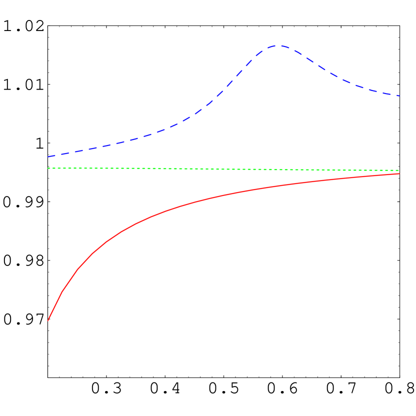
Figure 7: The separate factors, the solid line is the kinematic $\beta_{+-}^{3}/\beta_{00}^{3}$ and the dashed line the isospin corrections to the form-factors. Figure from ${}^{\ref{CEN}}$.

We could start by a naive attempt and simply use a constituent quark loop. This has been done in [37] with the result

$$a_{\mu}^{LL}(CQ)=60(4)~{}10^{-11}\,.$$ (11)

How much can we trust these numbers ? Using the result for the vacuum polarization

$$a_{\mu}^{q}(CQ)=\alpha^{2}Q_{q}^{2}m_{\mu}^{2}/(15\hat{m}_{q}^{2}\pi^{2})+\ldots$$ (12)

we obtain $\sim 2000~{}10^{-11}$ versus the result of $\sim 7000~{}10^{-11}$ using the data and the dispersive method. We can thus obviously not trust the result (12) and need hadronic inputs. This is not a CHPT calculation as often stated, in pure CHPT we encounter divergent contributions that necessitate a counterterm which is precisely the quantity we are trying to predict.

The problem of doublecounting hadronic and quark-loop contributions was alleviated very much by de Rafael[38] who noted that large $N_{c}$ counting and chiral powercounting could be used a a guide to classify them. He noted that the three main contributions are

1. ${\cal O}(N_{c})$ and $p^{6}$: $\pi^{0},\eta,\eta^{\prime}$ exchange.

2. ${\cal O}(N_{c})$ and $p^{8}$: irreducible four-meson vertices and exchanges of heavier resonances.

3. ${\cal O}(1)$ and $p^{4}$: $\pi^{+},K^{+}$ loop .

Figure 8: The hadronic light-by-light contribution to the muon anomalous magnetic moment.

This method was then applied by two groups, Hayakawa and Kinoshita HK(S)[39] and Bijnens, Pallante and Prades (BPP)[40]. The results are shown in Table 2.

$10^{11}a_{\mu}$	BPP	HK(S)
1	$-$85(13)	$-$83(6)
2	12(6)	8(11)
3	$-$19(13)	$-$4.5(8.1)
sum	$-$92(32)	$-$79(15)

Table 2: The three classes of contributions to the hadronic light-by-light for $a_{\mu}$ as obtained by the two groups.

For contribution 1, the two groups are in good agreement. Uncertainties here are the choices of formfactors, in practice what both groups have chosen amounts to double VMD, i.e., vector meson propagators are added in both photon legs in the $\pi^{0},\eta,\eta^{\prime}$ coupling to $\gamma\gamma$. There are basically no data with both photons off-shell, we need double tagged data at intermediate values of the photon off-shellness and data on $\eta$ and $\eta^{\prime}$ decays to two lepton pairs, i.e. on $\gamma^{*}\gamma^{*}\longleftrightarrow\pi^{0},\eta,\eta^{\prime}$. A preliminary study of the effects of various form factors on $a_{\mu}$ and how they can be observed in the other experiments can be found in [41], which yielded $a_{\mu}(1)=-88(9)~{}10^{-11}$.

For contribution 2, there are many small contributions with alternating signs, including scalar and axial-vector exchange.

The third contribution is different in both approaches because the choice of the underlying $\gamma^{*}\gamma^{*}\pi^{+}\pi^{-}$ vertex is different, both choices satisfy chiral constraints. Both are possible and this difference is at present inherent and provides a lower bound on the error. We need information on $\gamma^{*}\gamma^{*}\to\pi^{+}\pi^{-}$ at intermediate to large off-shellness for both photons to clarify this issue.

The matching of hadronic and short-distance results was studied in an approximative way in [40] and found to be satisfactory.

Numerically the total contribution is dominated by the relatively well understood pseudoscalar exchange. Given the complexity of the underlying amplitude it is difficult to prove that no major contribution has been missed but all additional effects studied in [39, 40] were relatively small. The errors in [40] were added linearly since all contributions involve fairly similar assumptions and is in my opinion reasonable. Unless a qualitatively different contribution from the ones included in these two calculations is discovered I do not expect the results to change significantly.

8 Structure of CHPT

8.1 History and overview

The structure of effective Lagrangians for the pseudoscalar mesons was originally worked out by Weinberg for two flavours and then generalized to arbitrary symmetry groups.[42] Weinberg[6] introduced the full EFT formalism which was then systematized and extended by Gasser and Leutwyler.[7, 8] The number of parameters was two at tree level and ten more at one-loop level. A first attempt at classifying the next order was done in [43] and later finished by [44]. The latter group also worked out the full infinity structure at two-loop order.[45]

In the abnormal parity sector, including one power of $\epsilon^{\mu\nu\alpha\beta}$, the lowest order is $p^{4}$ and is the celebrated Wess-Zumino-Witten term with no free parameters.[46] The methods of going beyond lowest order were worked out in [47] and work is going on to determine the precise number of parameters here.[49]

The extension to the nonleptonic weak sector was done by Kambor et al[48] and to the quenched approximation by Sharpe, Bernard and Golterman after early work by Morel.[50]

Some indication of the amount of work done in this area is given in Table 3 where we indicated the different Lagrangians people have considered and their number of parameters in parentheses. Recent lectures covering various aspects are [2].

${\cal L}_{\rm chiral\;order}$  ( $\#$ of LECs)	loop order
${\cal L}_{p^{2}}({2})$+${\cal L}_{p^{4}}^{\rm odd}({0})$+ ${\cal L}_{G_{F}p^{2}}^{\Delta S=1}({2})$ +${\cal L}_{e^{2}p^{0}}^{\rm em}({1})$ +${\cal L}_{G_{8}e^{2}p^{0}}^{\rm emweak}({1})$ +${\cal L}_{p}^{\pi N}({1})$+${\cal L}_{p^{2}}^{\pi N}({7})$	$L=0$
+${\cal L}_{G_{8}p^{0}}^{MB,\Delta S=1}({2})$+ ${\cal L}_{G_{8}p}^{MB,\Delta S=1}({8})$ + ${\cal L}_{e^{2}p^{0}}^{\pi N,{\rm em}}({3})$
+${{\cal L}_{p^{4}}^{\rm even}({10})}$ +${{\cal L}_{p^{6}}^{\rm odd}({23})}$ +${{\cal L}_{G_{8}p^{4}}^{\Delta S=1}({22})}$ +${{\cal L}_{e^{2}p^{2}}^{\rm em}({14})}$ +${{\cal L}_{G_{8}e^{2}p^{2}}^{\rm emweak}({14})}$ +${{\cal L}_{e^{2}p}^{\rm leptons}({5})}$	$L=1$
+${{\cal L}_{p^{3}}^{\pi N}({23})}$+ ${{\cal L}_{p^{4}}^{\pi N}({114})}$ +${{\cal L}_{G_{8}p^{2}}^{MB,\Delta S=1}({?})}$ +${{\cal L}_{e^{2}p}^{\pi N,{\rm em}}({8})}$
+${{\cal L}_{p^{6}}^{\rm even}({90})}$	$L=2$

Table 3: The standard model Lagrangian at low energies or an overview of the various Chiral Lagrangians and their number of parameters in parentheses, taken from ${}^{\ref{Ecker}}$.

8.2 Parameter Estimates

As can be seen from Table 3 one of the major problems in dealing with chiral Lagrangians is the number of free parameters. The reason is that we only use the chiral symmetry, $SU(3)_{L}\times SU(3)_{R}$, and its Goldstone character, all the remaining physics is parametrized.

First estimates of these parameters were done by using resonance exchange.[51] The conclusion is that the values of the $p^{4}$ parameters, $L_{i}^{r}$ are dominated by the vector and axial-vector degrees of freedom. Whenever these dominate, predictions work well. In the scalar sector qualitative agreement was obtained but the numerical agreement was less accurate. Later work concentrated on checking quark models in particular the chiral quark model[52], the Nambu-Jona-Lasinio model and extensions[53] and nonlocal quark models. Unfortunately, in the latter case the number of free parameters becomes rather large again. More recent work has concentrated on including more resonances and a more systematic use of short-distance constraints first started in[54]. Recent work is [55].

9 CHPT in the three flavour sector

Most basic two-loop calculations are done but a study of many smaller processes remains to be done. Finished ones include the vector and axial-vector two-point functions, masses and decay constants[56, 57], the latter also including isospin violation,[58] and the scalar two-point function[59].

The process $K\to\pi\pi\ell\nu$ is also known to this order,[60] because it is needed to determine the parameters. The results for the parameters that are known to two-loop order is in Table 4. I have quoted here the results from[58] using the new data[15] rather than the original fit[60] which only used the older data.[17] For pion and kaon vector formfactors partial results exist.[61, 62]

i	1	2	3	5	7	8
$10^{3}L_{i}^{r}(m_{\rho})$	$0.43(12)$	$0.73(12)$	$-2.35(37)$	$0.97(11)$	$-0.31(14)$	$0.60(18)$
$p^{4}$	0.38	1.59	$-2.91$	1.46	-0.49	1.00

Table 4: A fit to two-loop order of the $p^{4}$ CHPT parameters, table from ${}^{\ref{ABT3}}$.

Some of the two-loop corrections are fairly sizable, especially in the masses. The effect on mass ratios is smaller but claims have been made that this indicates a GCHPT picture in the three flavour case.

10 Quark Mass Ratios

One of the main results of the isospin breaking at two-loops so far is a new determination of the quark mass ratio[58] $m_{u}/m_{d}$

$${m_{u}}/{m_{d}}=0.46\pm 0.09\,.$$ (13)

and the pion mass splitting from quark masses

$$\left(m_{\pi^{\pm}}-m_{\pi^{0}}\right)_{\mbox{QCD}}=0.32\pm 0.20~{}\mbox{MeV}\,.$$

The uncertainty is larger than the usually quoted one since at two-loop level the uncertainty due to choices of saturation scale etc. were larger. We need at the present level $m_{s}/(m_{u}+m_{d})$ as an input parameter. The variation due to this is shown in Fig. 9. The main reason of the change w.r.t. the old values is the much larger estimate of the electromagnetic part of the Kaon mass difference.[63]

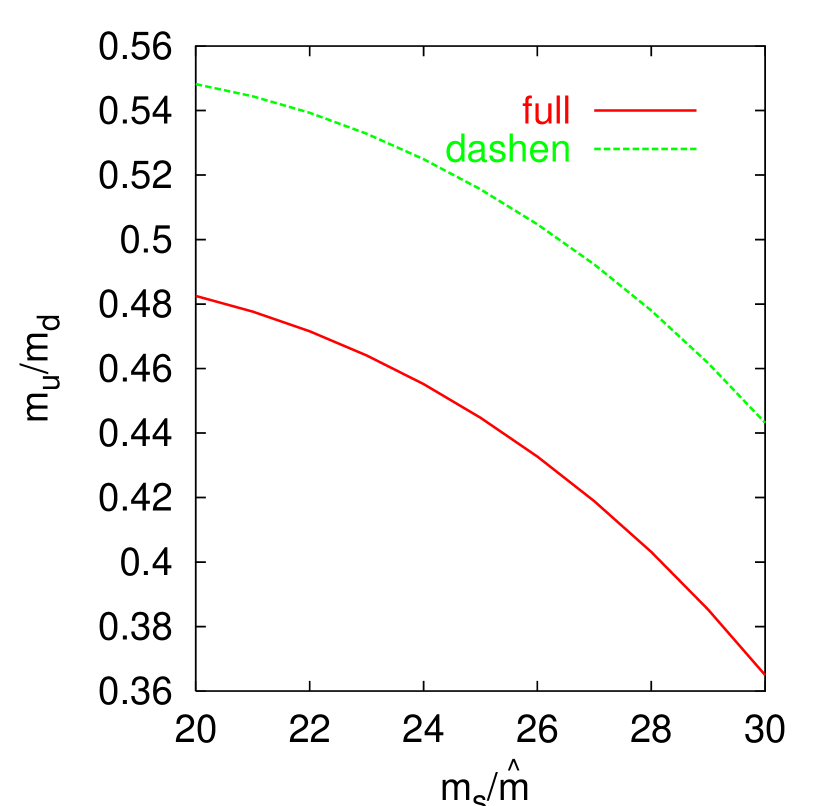
Figure 9: The variation of $m_{u}/m_{d}$ with $2m_{s}/(m_{u}+m_{d})$. The top line is using the old estimate for the electromagnetic Kaon mass difference. The bottom line uses the newer ones. From ${}^{\ref{ABT3}}$.

The uncertainty due to the Kaplan-Manohar ambiguity[64] is fixed due to the limits on $L_{4}^{r}$ and $L_{6}^{r}$ obtained from [59]. Note that the values for $L_{7}^{r}$ obtained are in perfect agreement with the arguments of [65] used to exclude the option $m_{u}=0$ there. That $m_{u}/m_{d}$ never gets near zero is shown in Fig. 10 where the range shown is significantly larger than allowed by[59].

11 Determination of $V_{us}$ (and $V_{ud}$)

The CKM matrix-element $V_{us}(V_{ud})$ can be determined from the decays $K\to\pi\ell\nu$ ($\pi^{+}\to\pi^{0}e^{+}\nu$) and hyperon semileptonic decays (neutron or nuclear $\beta$ decays). The underlying principle is always that a conserved vector current is 1 at $q^{2}=0$. The problem is now to calculate the correction to this from electromagnetism and quark masses.

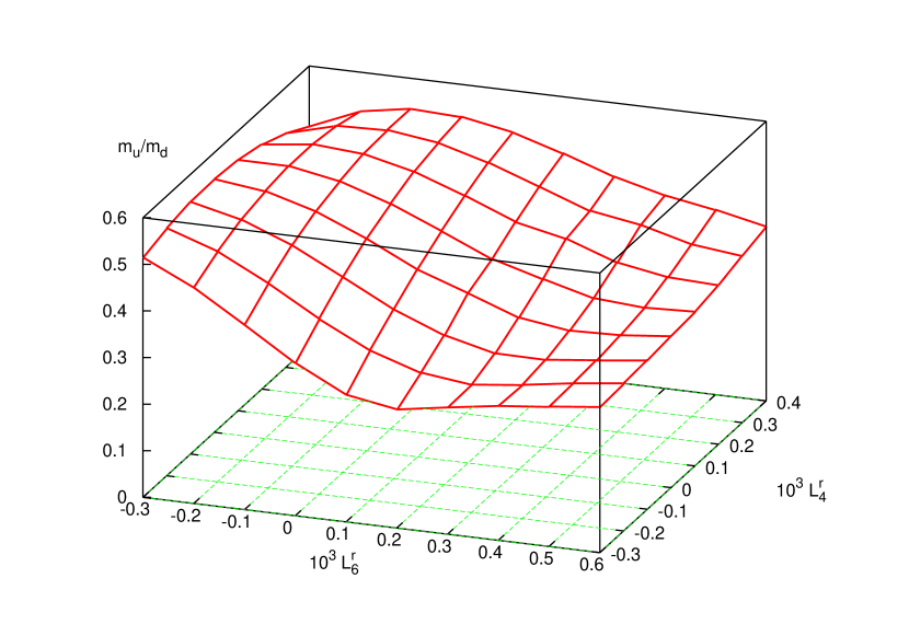
Figure 10: The variation of $m_{u}/m_{d}$ with the large $N_{c}$ suppressed input assumptions. Note that it never gets near zero, from ${}^{\ref{ABT3}}$.

For $V_{us}$ the vector current is $\bar{s}\gamma_{\mu}u$ so corrections are $(m_{s}-m_{u})^{2}$ not $(m_{d}-m_{u})^{2}$, (Ademollo-Gatto theorem[66]) and there is a sizable extrapolation to the zero-momentum point. For $V_{ud}$ the main problem is that we want an extremely high precision in neutron or pion $\beta$ decay which is hard to obtain or we have to theoretically understand nuclear effects to a very high precision.

A $V_{us}$ determination via hyperon $\beta$-decays has large theoretical problems. CHPT calculations suffer from large higher orders and many parameters. Not understood is why lowest order CHPT with model corrections works OK. References can be found in the particle data book. This area needs theoretical work very badly.

The experimental result

$$|V_{us}|=0.2196\pm 0.0023$$ (14)

together with $|V_{ud}|=0.9735\pm 0.0008$ yields

$$|V_{ud}|^{2}+|V_{us}|^{2}=0.9959\pm 0.0026$$ (15)

and a mild problem for the unitarity of the CKM matrix.

The theory[67] and data behind Kaon $\beta$-decays are both old by now. The data we expect to improve in the near future with data from BNL, KLOE, KTeV, NA48 and possibly others. The theory consists of oldfashioned photon loops and one-loop CHPT calculations for the quark mass effects. The former are in the process of being improved by Cirigliano et al. and the latter extended to two-loops[62]. We can thus expect an improved accuracy for $V_{us}$ in the next few years. GCHPT allows for larger quark mass effects[68] than the calculation of [67].

12 Anomalies

The most celebrated result here is $\pi^{0}\to\gamma\gamma$. Good agreement with the anomaly prediction exists, at the two sigma level, but we need to push both theory and experiment beyond the present experimental precision of $7.8\pm 0.6$ eV.

Similarly in $\eta\to\gamma\gamma$. The discrepancy between $e^{+}e^{-}$ and Primakoff measurements persists. KLOE should be able to contribute significantly here. Data for $\pi^{0},\eta,\eta^{\prime}\longleftrightarrow\gamma^{*}\gamma^{*}$ are needed for $a_{\mu}$ as discussed above and for $\eta\to\ell^{+}\ell^{-}$, even if in the latter case differences are smaller.

$\gamma\pi\to\pi\pi$ experiment is significantly above theory, corrections go in the right direction but only halfway (one-loop[69] dispersive[70]). New experiments at JLab and possibly at COMPASS are planned. A possible problem are the radiative corrections[71]. In $\eta\to\pi^{+}\pi^{-}\gamma$ the agreement between theory[69] and experiment is satisfactory. Kaon decays $K\to\gamma\ell\nu,\pi\pi\ell\nu,\pi\gamma\ell\nu$ allow more tests in particular also of the sign and of the quark mass dependence of the anomalous effects. One example is discussed below.

13 More $\eta$

In $\eta$-decays there are more interesting results. The decays $\eta\to\pi^{+}\pi^{-}\pi^{0},\pi^{0}\pi^{0}\pi^{0}$ play a role in the determination of the quark masses since its decay width is $\Gamma\sim(m_{u}-m_{d})^{2}\overline{\Gamma}$. The present comparison with theory is shown in Table 5.

Exp.:	$280\pm 28$ eV
$p^{2}$	66 eV	Ref. [72]
$p^{4}$	$167\pm 50$ eV	Ref. [73]
dispersive	$209\pm 20$ eV	Ref. [74]

Table 5: Comparison of theory and experiment for $\eta\to\pi\pi\pi$.

With a slightly larger value of $m_{d}-m_{u}$, which is in fact obtained as discussed above, we obtain good agreement. A possible problem is that the dispersive calculations use, and can be checked using, the Dalitz-plot parameters. As an example, $-10^{3}\alpha$ in the neutral decay was obtained in[74] as $7\pm 7$. Data are $22\pm 23$ (GAMS[75]), $52\pm 18$ (Crystal Barrel[76]) and a preliminary result by the Crystal Ball of $26\pm 6$. We expect more data here in the near future from KLOE, WASA and the Crystal Ball as well as for the charged decays. Should this discrepancy in the Dalitz plot parameters persist a reanalysis will become necessary.

The process $\eta\to\pi^{0}\gamma\gamma$ provides a good test of $p^{6}$ CHPT and VMD with a width prediction of $0.40(20)~{}$eV[77], present experiment gives $0.84(19)~{}$eV[75].

14 Rare semileptonic decays

Many calculations exist. See e.g. the talk by Isidori and the proceedings of KAON99. An example is the recently improved precision on the form-factors in $K\to\mu\nu\gamma$ by the BNL-E787 experiment[78]. The structure dependent terms have been measured to be

$$|F_{V}+F_{A}|^{\mbox{exp}} = 0.165(0.155)\pm 0.013\quad[0.14]$$

$$|F_{V}-F_{A}|^{\mbox{exp}} = 0.102(0.065)\pm 0.085\quad[0.05]$$

The difference in the numbers with and without brackets is due to assumptions on the $W^{2}$ dependence. The theory numbers in square brackets are $p^{4}$ results from [79]. Again, improvement to the $p^{6}$-level is needed.

15 Nonleptonic decays: CHPT

This area was pioneered by [48] and one of its major results is the chiral symmetry tests in $K\to\pi\pi$ and $K\to\pi\pi\pi$ decays. Various relations have been produced[80] and their comparison with experiment is given in Table 6. The overall agreement is satisfactory but the newer CPLEAR data and effects of order $m_{\pi}^{2}$ have not been incorporated and obviously the $\Delta I=3/2$ need experimental improvement.

$$\begin{array}[]{|c|ccc|}\hline\cr&p^{2}&p^{4}&\mbox{experiment}\\ \hline\cr\alpha_{1}&74&\mbox{input}^{\dagger}&91.71\pm 0.32\\ \beta_{1}&-16.5&\mbox{input}^{*}&-25.68\pm 0.27\\ \zeta_{1}&&-0.47\pm 0.18^{\dagger}&-0.47\pm 0.15\\ \xi_{1}&&-1.58\pm 0.19^{*}&-1.51\pm 0.30\\ \alpha_{3}&-4.1&\mbox{input}^{\bullet}&-7.36\pm 0.47\\ \beta_{3}&-1.0&\mbox{input}^{\blacktriangle}&-2.42\pm 0.41\\ \gamma_{3}&1.8&\mbox{input}^{o}&2.26\pm 0.23\\ \xi_{3}&&0.092\pm 0.030^{\blacktriangle}&-0.12\pm 0.17\\ \xi_{3}^{\prime}&&-0.033\pm 0.077^{o}&-0.21\pm 0.51\\ \zeta_{3}&&-0.011\pm 0.006^{\bullet}&-0.21\pm 0.08\\ \hline\cr\end{array}$$

Table 6: Chiral symmetry relations for various Dalitz plot parameters in $K\to 3\pi$ and their comparison with experiment. The relations are indicated using the different superscripts.

In rare decays there are many successful predictions. An example is the prediction[81] and subsequent confirmation of $K_{S}\to\gamma\gamma$. New results on this decay can be found in the KTeV and NA48 rare decay talks.

Similar predictions exist for $K_{L}\to\pi^{0}\gamma\gamma$ and $K\to\pi\gamma^{*}$ and $K\to\pi Z^{*}$. A problem case is the decay $K_{L}\to\gamma\gamma$ which is plagued by strong cancellations but very good predictions exists for the various $K\to\pi\nu\bar{\nu}$ modes. Reviews are the talk by Isidori here and at KAON99.

16 Nonleptonic decays and $\epsilon^{\prime}/\epsilon$

The theoretical precision of $\epsilon^{\prime}/\epsilon$ is now way behind the experimental determination reported here by KTeV and NA48. I will only comment the approaches using chiral Lagrangian related methods as a main tool. In particular I concentrate on the various analytical approaches using large $N_{c}$ as a guide.

The major problem is that due to the virtual $W$-bosons we need an integration over all scales. The short-distance part can be resummed using renormalization group methods and is known to two-loops, calculated by two groups who are in perfect agreement, see [82] for recent lectures and references.

The large $N_{c}$ approach combined with CHPT was pioneered by Bardeen et al.[83] and is now used by several groups. The Dortmund[84] group uses pure CHPT at long distances and matches it directly onto short-distance QCD, the Granada-Lund[85] group uses the $X$-boson method to match correctly onto the short-distance schemes and the ENJL model to improve on the hadronic picture at intermediate scales. Finally the Valencia group[86] uses a semi-phenomenological approach to calculate $\epsilon^{\prime}/\epsilon$. It should be noted that the Dortmund and Granada-Lund groups also reproduce within the uncertainties of their approach the $\Delta I=1/2$ rule which no other method can claim so far.

Besides these calculations which fully predict $\epsilon^{\prime}/\epsilon$ there has been major progress on several fronts recently. In particular it has been realized that $B_{7}$ and $B_{8}$ can be studied in the chiral limit from $\tau$-decay data.[89, 90] All groups basically agree in the method but differ in the treatment of scheme-dependence and error estimates due to the spectral functions from $\tau$ data. Comparison of these results with the calculations mentioned above is in.[90] Similar dispersive results for the $B_{K}$ parameter[91] were in reasonable agreement with the equivalent Granada-Lund one[85, 92].

Calculations with no good theory for the long-distance–short-distance matching have not been included here. In particular I included neither the factorization (Taipei) nor the chiral quark model (Trieste[87]) results.

The estimates of $\epsilon^{\prime}/\epsilon$ shown in Table 7, increased significantly due to three effects:

• $\Omega_{IB}$ has gone down, removing part of the cancellations due to isospin breaking.[93]

• Final state interactions should be included both in the real and in the imaginary parts.[87] Typically the real part was treated experimentally and the imaginary part to order $p^{2}$. Correcting this produces a strong enhancement.[87, 88] Criticisms now focus on the size of this effect not its existence.

• Large, not fully understood, non-factorizable corrections[85] to $B_{6}$.

	$10^{4}\epsilon^{\prime}/\epsilon$
Granada-Lund	$34\pm 18$
Dortmund	$11\pm 5$
Valencia	$17\pm 9$
Data	$17.2\pm 1.8$

Table 7: Some predictions for $\epsilon^{\prime}/\epsilon$ and the the data.

17 Baryons

Baryons, hyperons and nuclei are also areas where chiral Lagrangians play an important role. The one baryon sector was reviewed in,[4] many more results can be found in the proceedings of Chiral Dynamics 2000 at JLab.

In the two or more nucleon sector some recent progress has been obtained by the advent of a proper power-counting[94]. Many applications can be found in the abovenamed proceedings and in the review.[5] I only quote two examples relevant for cosmology and solar physics. The EFT calculation[95] allowed to reduce the uncertainty for deuteron break-up in the early universe from 5% to 1%. More importantly, good data at one point will improve the prediction over the whole relevant energy range. The cross-section is shown in Fig. 11.

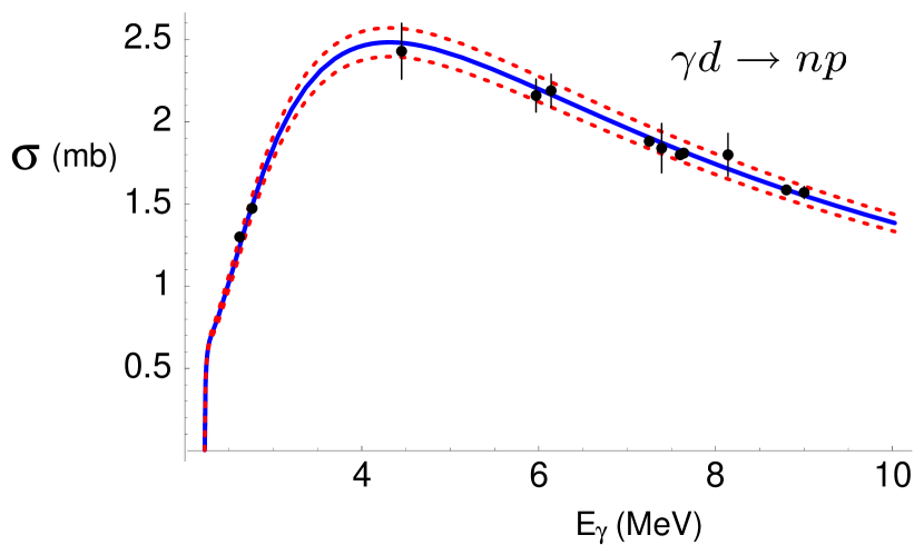
Figure 11: The cross-section relevant for deuteron breakup from EFT, figure from ${}^{\ref{Chen}}$.

For the cross-section of the main solar proton fusion process $pp\to de^{+}\nu$ EFT methods allow a one parameter prediction.[96] A 10% measurement of $\bar{\nu}_{e}d$ scattering at a reactor allows a 3% prediction of the $pp$ rate.

18 Colour Superconductivity

At very high baryon densities a new phase of QCD is expected to appear[97] where we get diquark condensation in the anti triplet colour channel of $3_{c}\times 3_{c}$ rather than in the colour singlet quark-antiquark in $3_{c}\times\bar{3}_{c}$ of the usual QCD vacuum. This phase has colour-flavour locking due to the nature of the condensate and the symmetries are broken in the pattern

$$SU(3)_{c}\times SU(3)_{L}\times SU(3)_{R}\times U_{V}(1)$$

$$\Rightarrow SU(3)_{c+L+R}\times Z_{2}(q\to-q)$$ (16)

This results in 8 massive gluons, 8 Left-Right Goldstone Bosons, one Baryon-number Goldstone Boson. This looks very much like the spectrum of 8 vectors and 8 pseudoscalars in the usual QCD vacuum. Indeed the whole formalism of EFT can also be used here as can be seen in the review by Alford.[98] Some peculiarities are that the mass spectrum is quadratic in the quark masses due to the $Z_{2}$ symmetry of the condensate and that instead of the more familiar photon-rho mixing we now have photon gluon mixing.[99]

19 Not covered

A few more areas with recent progress are

• The question of large $N_{f}$ and GCHPT.[100]

• $\eta$-$\eta^{\prime}$ mixing.[101]

• Phenomenological Chiral Lagrangians in resonance decays especially $\phi$-decays and $\tau$ phenomenology.[102]

• CHPT in the single baryon sector.[4, 103]

• CHPT for vector mesons.[104]

• Resummation work beyond the ones discussed here.[105]

• Connection with lattice QCD: the use of CHPT to extrapolate lattice results to physical quark masses and study effects of (partial) quenching and finite volume.

20 Conclusions

I hope to have convinced you that the field of Chiral Lagrangians is very active and has many applications with relevance for a wide spectrum of phenomena in high-energy and nuclear physics.

References

- [1]
- [2] G. Colangelo and G. Isidori, hep-ph/0101264; H. Leutwyler, hep-ph/0008124; A. Pich, hep-ph/9806303; Rept. Prog. Phys. 58, 563 (1995) [hep-ph/9502366]; G. Ecker, Prog. Part. Nucl. Phys. 35, 1 (1995) [hep-ph/9501357]; J. Bijnens, Int. J. Mod. Phys. A8, 3045 (1993) and [3, 4, 5].
- [3] G. Ecker, hep-ph/0011026.
- [4] V. Bernard et al.,Int. J. Mod. Phys. E4, 193 (1995) [hep-ph/9501384].
- [5] S. R. Beane et al., nucl-th/0008064.
- [6] S. Weinberg, Physica A96, 327 (1979).
- [7] J. Gasser and H. Leutwyler, Annals Phys. 158, 142 (1984).
- [8] J. Gasser and H. Leutwyler, Nucl. Phys. B 250, 465 (1985).
- [9] N. H. Fuchs et al.,Phys. Lett. B269, 183 (1991); M. Knecht and J. Stern, hep-ph/9411253.
- [10] S. Weinberg, Phys. Rev. Lett. 17, 616 (1966).
- [11] J. Gasser and H. Leutwyler, Phys. Lett. B 125, 325 (1983).
- [12] J. Bijnens et al., Phys. Lett. B 374, 210 (1996) [hep-ph/9511397]; Nucl. Phys. B 508, 263 (1997) [hep-ph/9707291].
- [13] M. Knecht et al., Nucl. Phys. B 457, 513 (1995) [hep-ph/9507319].
- [14] B. Ananthanarayan et al., hep-ph/0005297, to be published in Phys. Rept..
- [15] S. Pislak et al. [BNL-E865 Coll.], hep-ex/0106071.
- [16] G. Colangelo et al., Phys. Rev. Lett. 86, 5008 (2001) [hep-ph/0103063]; Nucl. Phys. B603, 125 (2001) [hep-ph/0103088].
- [17] L. Rosselet et al., Phys. Rev. D15, 574 (1977).
- [18] F. Gomez et al. [DIRAC Coll.], Nucl. Phys. Proc. Suppl. 96, 259 (2001).
- [19] J. Gasser et al.,Phys. Rev. D64, 016008 (2001) [hep-ph/0103157]. V. Antonelli et al.,Annals Phys. 286, 108 (2001) [hep-ph/0003118].
- [20] S. Bellucci et al.,Nucl. Phys. B423, 80 (1994) [Erratum B431, 413 (1994)] [hep-ph/9401206].
- [21] U. Bürgi, Nucl. Phys. B 479, 392 (1996) [hep-ph/9602429].
- [22] J. Bijnens and P. Talavera, Nucl. Phys. B 489, 387 (1997) [hep-ph/9610269].
- [23] J. Bijnens et al.,JHEP 9805, 014 (1998) [hep-ph/9805389].
- [24] F. Guerrero and A. Pich, Phys. Lett. B 412, 382 (1997) [hep-ph/9707347]; A. Pich and J. Portoles, Phys. Rev. D 63, 093005 (2001) [hep-ph/0101194].
- [25] T. N. Truong, hep-ph/0001271.
- [26] R. Barate et al. [ALEPH Coll.], Z. Phys. C 76, 15 (1997).
- [27] S. Anderson et al. [CLEO], Phys. Rev. D 61, 112002 (2000) [hep-ex/9910046].
- [28] S. R. Amendolia et al. [NA7 Coll.], Nucl. Phys. B 277, 168 (1986).
- [29] S. R. Amendolia et al., Phys. Lett. B 138, 454 (1984).
- [30] H. N. Brown et al., Phys. Rev. D 62, 091101 (2000) [hep-ex/0009029]; Phys. Rev. Lett. 86, 2227 (2001) [hep-ex/0102017]; J.Miller, these proceedings
- [31] A. Czarnecki and W. J. Marciano, Nucl. Phys. Proc. Suppl. 76, 245 (1999) [hep-ph/9810512].
- [32] K. Melnikov, hep-ph/0105267.
- [33] S. Peris et al.,Phys. Lett. B 355, 523 (1995) [hep-ph/9505405].
- [34] See e.g. F. Jegerlehner, hep-ph/0104304.
- [35] J. F. De Troconiz and F. J. Yndurain, hep-ph/0106025.
- [36] V. Cirigliano et al.,hep-ph/0104267.
- [37] T. Kinoshita et al.,Phys. Rev. D 31, 2108 (1985).
- [38] E. de Rafael, Phys. Lett. B 322, 239 (1994) [hep-ph/9311316].
- [39] M. Hayakawa et al., Phys. Rev. Lett. 75, 790 (1995) [hep-ph/9503463]; Phys. Rev. D54, 3137 (1996) [hep-ph/9601310]; Phys. Rev. D57, 465 (1998) [hep-ph/9708227].
- [40] J. Bijnens et al.,Phys. Rev. Lett. 75, 1447 (1995) [Erratum 75, 3781 (1995)] [hep-ph/9505251]; Nucl. Phys. B 474, 379 (1996) [hep-ph/9511388].
- [41] J. Bijnens and F. Persson, hep-ph/0106130.
- [42] S. Coleman et al.,Phys. Rev. 177 (1969) 2239; C. G. Callan et al.,Phys. Rev. 177 (1969) 2247.
- [43] H. W. Fearing and S. Scherer, Phys. Rev. D53, 315 (1996) [hep-ph/9408346].
- [44] J. Bijnens et al.,JHEP 9902, 020 (1999) [hep-ph/9902437].
- [45] J. Bijnens et al.,Annals Phys. 280, 100 (2000) [hep-ph/9907333].
- [46] J. Wess and B. Zumino, Phys. Lett. B 37, 95 (1971); E. Witten, Nucl. Phys. B 223, 422 (1983).
- [47] D. Issler, SLAC-PUB-4943-REV; J. Bijnens, A. Bramon and F. Cornet, Z. Phys. C 46, 599 (1990). R. Akhoury and A. Alfakih, Annals Phys. 210, 81 (1991).
- [48] J. Kambor et al.,Nucl. Phys. B346, 17 (1990).
- [49] J. Bijnens, L. Girlanda and P. Talavera, work in progress.
- [50] A. Morel, SACLAY-PhT/87-020, J. de Phys. A, 48, 111 (1987); S. R. Sharpe, Phys. Rev. D41, 3233 (1990). C. W. Bernard and M. F. Golterman, Phys. Rev. D46, 853 (1992) [hep-lat/9204007].
- [51] G. Ecker et al.,Nucl. Phys. B321, 311 (1989).
- [52] D. Espriu et al.,Nucl. Phys. B 345, 22 (1990) [Erratum B 355, 278 (1990)].
- [53] J. Bijnens et al.,Nucl. Phys. B390, 501 (1993) [hep-ph/9206236].
- [54] G. Ecker et al.,Phys. Lett. B223, 425 (1989).
- [55] O. Cata and S. Peris, hep-ph/0107062; M. Golterman and S. Peris, JHEP 0101, 028 (2001) [hep-ph/0101098]; S. Peris et al.,JHEP 9805, 011 (1998) [hep-ph/9805442]; M. Knecht and A. Nyffeler, hep-ph/0106034.
- [56] E. Golowich and J. Kambor, Nucl. Phys. B447, 373 (1995) [hep-ph/9501318]; Phys. Rev. D58, 036004 (1998) [hep-ph/9710214].
- [57] G. Amoros et al.,Nucl. Phys. B 568, 319 (2000) [hep-ph/9907264].
- [58] G. Amoros et al.,Nucl. Phys. B 602, 87 (2001) [hep-ph/0101127].
- [59] B. Moussallam, Eur. Phys. J. C 14, 111 (2000) [hep-ph/9909292].
- [60] G. Amoros et al.,Phys. Lett. B 480, 71 (2000) [hep-ph/9912398]; Nucl. Phys. B 585, 293 (2000) [Erratum B 598, 665 (2000)] [hep-ph/0003258].
- [61] P. Post and K. Schilcher, Phys. Rev. Lett. 79, 4088 (1997) [hep-ph/9701422]; Nucl. Phys. B 599, 30 (2001) [hep-ph/0007095].
- [62] J. Bijnens and P. Talavera, in progress.
- [63] J. F. Donoghue et al.,Phys. Rev. Lett. 69, 3444 (1992); Phys. Rev. D 47, 2089 (1993); J. Bijnens, Phys. Lett. B 306, 343 (1993) [hep-ph/9302217]; J. Bijnens and J. Prades, Nucl. Phys. B 490, 239 (1997) [hep-ph/9610360].
- [64] D. B. Kaplan and A. V. Manohar, Phys. Rev. Lett. 56, 2004 (1986).
- [65] H. Leutwyler, Nucl. Phys. B337, 108 (1990).
- [66] R.E. Behrends and A. Sirlin, Phys. Rev. Lett. 4, 186 (1960); M. Ademollo and R. Gatto, Phys. Rev. Lett. 13,264(1964).
- [67] H. Leutwyler and M. Roos, Z. Phys. C 25, 91 (1984).
- [68] N. H. Fuchs et al.,Phys. Rev. D62, 033003 (2000) [hep-ph/0001188].
- [69] J. Bijnens et al.,Phys. Lett. B237, 488 (1990).
- [70] B. Holstein, Phys. Rev. D53, 4099 (1996) [hep-ph/9512338]; T. Hannah, Nucl. Phys. B593, 577 (2001) [hep-ph/0102213]. T. Truong, hep-ph/0105123.
- [71] L. Ametller et al., hep-ph/0107127.
- [72] J. Cronin, Phys. Rev. 161 (1967) 1483.
- [73] J. Gasser and H. Leutwyler, Nucl. Phys. B 250, 539 (1985).
- [74] J. Kambor et al.,Nucl. Phys. B 465, 215 (1996) [hep-ph/9509374]; A. V. Anisovich and H. Leutwyler, Phys. Lett. B 375, 335 (1996) [hep-ph/9601237].
- [75] D. Alde et al. [GAMS], Z. Phys. C 25, 225 (1984) [Yad. Fiz. 40, 1447 (1984)].
- [76] A. Abele et al. [Crystal Barrel Coll.], Phys. Lett. B 417 (1998) 193.
- [77] L. Ametller et al.,Phys. Lett. B 276, 185 (1992).
- [78] S. Adler et al. [E787 Coll.], Phys. Rev. Lett. 85, 2256 (2000) [hep-ex/0003019].
- [79] J. Bijnens et al.,Nucl. Phys. B 396, 81 (1993) [hep-ph/9209261].
- [80] J. Kambor et al.,Phys. Lett. B 261, 496 (1991); J. Kambor et al.,Phys. Rev. Lett. 68, 1818 (1992).
- [81] J. L. Goity, Z. Phys. C 34, 341 (1987); G. D’Ambrosio and D. Espriu, Phys. Lett. B 175, 237 (1986).
- [82] A. J. Buras, hep-ph/9806471.
- [83] W. Bardeen et al., Phys. Lett. B 192, 138 (1987).
- [84] T. Hambye et al.,Nucl. Phys. B564, 391 (2000) [hep-ph/9906434]; Eur. Phys. J. C 10, 271 (1999) [hep-ph/9902334].
- [85] J. Bijnens and J. Prades, JHEP 9901, 023 (1999) [hep-ph/9811472]; 0001, 002 (2000)[hep-ph/9911392]; 0006, 035 (2000) [hep-ph/0005189].
- [86] E. Pallante et al.,hep-ph/0105011.
- [87] S. Bertolini et al., Nucl. Phys. B 514, 93 (1998) [hep-ph/9706260].
- [88] E. Pallante and A. Pich, Phys. Rev. Lett. 84, 2568 (2000) [hep-ph/9911233]; Nucl. Phys. B 592, 294 (2001) [hep-ph/0007208].
- [89] J. F. Donoghue and E. Golowich, Phys. Lett. B478, 172(2000) [hep-ph/9911309]; V. Cirigliano et al., JHEP 0010, 048 (2000) [hep-ph/0007196]; M. Knecht et al.,Phys. Lett. B 508, 117 (2001) [hep-ph/0102017].
- [90] J. Bijnens, E. Gamiz and J. Prades, hep-ph/0108240.
- [91] S. Peris and E. de Rafael, Phys. Lett. B 490, 213 (2000) [hep-ph/0006146].
- [92] J. Bijnens and J. Prades, Nucl. Phys. B 444, 523 (1995) [hep-ph/9502363].
- [93] G. Ecker et al., Phys. Lett. B 477, 88 (2000) [hep-ph/9912264].
-
[94]
D.B. Kaplan et al.,Phys. Lett. B424, 390(1998)[nucl-th/9801034];
Nucl. Phys.
B534, 329 (1998)[nucl-th/9802075]. - [95] J. Chen and M. J. Savage, Phys. Rev. C 60, 065205 (1999) [nucl-th/9907042].
- [96] M. Butler and J. Chen, nucl-th/0101017; X. Kong and F. Ravndal, Nucl. Phys. A 656, 421 (1999) [nucl-th/9902064].
- [97] B. C. Barrois, Nucl. Phys. B 129, 390 (1977). D. Bailin and A. Love, Phys. Rept. 107, 325 (1984). M. Alford et al.,Phys. Lett. B 422, 247 (1998) [hep-ph/9711395]. R. Rapp et al.,Phys. Rev. Lett. 81, 53 (1998) [hep-ph/9711396].
- [98] M. Alford, hep-ph/0102047.
- [99] R. Casalbuoni et al.,Phys. Rev. D 63, 114026 (2001) [hep-ph/0011394].
- [100] L. Girlanda et al.,Phys. Rev. Lett. 86, 5858 (2001) [hep-ph/0103221].
- [101] R. Kaiser and H. Leutwyler, Eur. Phys. J. C 17, 623 (2000) [hep-ph/0007101]. T. Feldmann et al.,Phys. Lett. B 449, 339 (1999) [hep-ph/9812269].
- [102] See e.g. the contributed paper by K. R. Nasriddinov et al.,hep-ph/0001276 and the KLOE contribution.
- [103] T. Becher and H. Leutwyler, Eur. Phys. J. C9, 643 (1999) [hep-ph/9901384]; JHEP 0106, 017 (2001) [hep-ph/0103263].
- [104] E. Jenkins et al., Phys. Rev. Lett. 75, 2272 (1995) [hep-ph/9506356]; J. Bijnens et al.,Nucl. Phys. B 501, 495 (1997) [hep-ph/9704212].
- [105] J. A. Oller et al.,Prog. Part. Nucl. Phys. 45, 157 (2000) [hep-ph/0002193].