CERN–TH/2001–216

  Abstract
We study 5 dimensional grand-unified theories in an orbifold geometry by the method of effective field theory: we match the low and high energy theories by integrating out at 1-loop the massive Kaluza-Klein states. In the supersymmetric case the radius dependence of threshold effects is fixed by the rescaling anomalies of the low energy theory. We focus on a recently proposed $SU(5)$ model on $M^{4}\times S^{1}/(Z_{2}\times Z_{2}^{\prime})$. Even though the spectrum of the heavy modes is completely known, there still are corrections to gauge unification originating from boundary couplings. In order to control these effects one has to rely on extra assumptions. We argue that, as far as gauge couplings are concerned, the predictive power of these models is similar to conventional GUTs.  

1 Introduction

Since their early days [1] grand unified theories (GUT) have attracted a lot of interest and though the paradigm is not flawless it is still an exciting and active research field. Besides aesthetic reasons, a strong evidence in favor of GUTs is that in the minimal supersymmetric standard model (MSSM) the couplings of $SU(3)\times SU(2)\times U(1)$ unify at a scale of order $10^{16}$ GeV [2]. Models with extra compact dimensions can add interesting twists to the basic GUT idea. This was first realized in string models where intrinsically higher dimensional mechanisms can solve some of the problems of conventional GUTs. One example is the doublet-triplet splitting problem [3]. Recently there has been a revival in extra-dimensional GUT model building, but now taking a “bottom-up” approach as opposed to the “top-down” approach of string model building. Kawamura has first constructed a non-supersymmetric model on $S^{1}/Z_{2}$ [4], and has later obtained a realistic supersymmetric spectrum on $S^{1}/(Z_{2}\times Z_{2}^{\prime})$ [5]. (The interesting properties of $S^{1}/(Z_{2}\times Z_{2}^{\prime})$ for model building where noticed in ref. [6]). The model was further studied in [7, 8]. Many papers have since followed [9]-[11]. In this paper we extend the effective field theory (EFT) approach proposed by Weinberg [12] to the case of a grand unified gauge theory in five dimensions. We build the effective field theory valid below the GUT scale by integrating out the heavy degrees of freedom represented here by the massive KK excitations. The form of the low-energy theory is strongly constrained by symmetries and operators’ coefficients are expressed in terms of the parameters of the underlying high energy theory. As an explicit example we consider the $SU(5)$ unified theory on $M^{4}\times S^{1}/(Z_{2}\times Z_{2}^{\prime})$ of ref. [5, 8]. We compute the matching functions relating the SM gauge couplings to the parameters of the 5 dimensional theory. Although the explicit results are given for $SU(5)$, the method presented is general. One important feature of the orbifold geometry is the presence at the boundary of local operators contributing to the vector boson kinetic term. These operators do not respect $SU(5)$ and lead to corrections to gauge unification. Indeed their coefficients follow a logarithmic RG evolution, so that they cannot just be set to zero.

The outline of the paper is the following. In section 2 we discuss the conditions under which the gauge symmetry does not conflict with the orbifold projections and the $SU(5)$ model considered is briefly reviewed. Section 3 is devoted to a general discussion of the boundary counterterms induced by quantum corrections at the orbifold fixed points. The construction of the effective 4D low energy theory is presented in section 4, in particular the matching functions are computed at the one loop level. Finally, in section 5, the values of the SM gauge couplings are computed at the weak scale at next to leading order and the phenomenological consequences are discussed.

2 $SU(5)$ on the orbifold

We consider a grand unified 5-dimensional $SU(5)$ theory defined on $M^{4}\times S^{1}/(Z_{2}\times Z_{2}^{\prime})$ [5, 8], where $S^{1}/(Z_{2}\times Z_{2}^{\prime})$ is obtained from a circle with radius $R$ by the following identifications:

$$Z_{2}:\quad y\sim 2\pi R-y\,,\qquad Z_{2}^{\prime}:\quad y\sim\pi R-y\,\qquad y\in[0,2\pi R].$$ (1)

Coordinates in 5D are denoted by $X^{M}=(x^{\mu},y)$, using capital Latin (small Greek) letters for 5D (4D) indices. The points $(0,\pi R)$ and $(\pi R/2,3\pi R/2)$ are fixed under the action of $Z_{2}$ and $Z_{2}^{\prime}$ respectively; moreover $0\sim\pi R$ and $\pi R/2\sim 3\pi R/2$.

A function $f(x,y)$ with a definite parity under the orbifold projections can be Fourier decomposed according to

$$f(x,y)=\sum_{n=0}^{+\infty}f^{(n)}(x)\,\Psi_{n}(y),\qquad\Psi_{n}(y)=\begin{cases}a_{2n}\,\cos\displaystyle{\frac{2ny}{R}}&\quad(+,+)\\[7.11317pt] a_{2n+1}\,\cos\displaystyle{\frac{(2n+1)y}{R}}&\quad(+,-)\\[7.11317pt] a_{2n+1}\,\sin\displaystyle{\frac{(2n+1)y}{R}}&\quad(-,+)\\[7.11317pt] a_{2n+2}\,\sin\displaystyle{\frac{(2n+2)y}{R}}&\quad(-,-)\end{cases}$$ (2)

$$a_{0}=\frac{1}{\sqrt{2\pi R}},\quad a_{n}=\frac{1}{\sqrt{\pi R}}\quad n\not=0\,.$$

Only a function with parity $(+,+)$ has a zero mode.

When a gauge theory is defined in a orbifold one has to satisfy certain consistency conditions in order to avoid that gauge symmetry conflicts with orbifold projections. The $Z_{2}$ action $P$ on the fields of the theory is defined to be

$$\Phi(x,y)\to\Phi(x,-y)=P\,\Phi(x,y)\qquad\qquad P^{2}=1\;,$$ (3)

where we have collected all the fields in single vector $\Phi$. Without loss of generality $P$ can be chosen diagonal with eigenvalues $\pm 1$. In particular, for the gauge field $A_{M}^{i}T^{i}$ one has

$$\begin{split}A_{\mu}^{i}(x,-y)&=\Lambda^{ij}A_{\mu}^{j}(x,y)\\ A_{5}^{i}(x,-y)&=-\Lambda^{ij}A_{5}^{j}(x,y)\end{split}\qquad\qquad\Lambda^{2}=1\quad;$$ (4)

where $T^{i}$ are the generators of the gauge group $G$ with structure constants $f_{ijk}$. For the Lagrangian to be $Z_{2}$ invariant, the covariant derivative acting on a matter field $D_{M}\varphi$ must have a definite transformation property under $Z_{2}$, thus

$$PT^{i}P=\Lambda^{ij}T^{j}$$ (5)

In turn this implies that $P$ is an inner automorphism of the Lie algebra ${\cal G}$ of $G$, in other words

$$\Lambda_{im}\,\Lambda_{jn}\,\Lambda_{kl}\,f_{mnl}=f_{ijk}\,,$$ (6)

and $P$ acts as a group conjugation (see [10] for a discussion of inner and outer automorphism in the context of orbifold projections). Taking $\Lambda_{ij}=\delta_{ij}\,c_{i}$ (no summation in $i$), with $c_{i}=\pm 1$, we can divide the generators in two subsets: ${\cal H}=\{T^{a},\,a=1,\,\cdots n\,:c_{a}=1\;\forall a\}$ and ${\cal V}=\{T^{\hat{a}},\,\hat{a}=n+1,\,\cdots\text{dim}({\cal G})\,:c_{\hat{a}}=-1\;\forall\hat{a}\}$. From eq.(6) it follows that $[{\cal H},{\cal H}]={\cal H}$, $[{\cal H},{\cal V}]={\cal V}$ and $[{\cal V},{\cal V}]={\cal H}$. Repeating the same argument, with the simplifying hypothesis that also second projection $Z_{2}^{\prime}$ acts through $P^{\prime}$ as a diagonal matrix on the fields, exactly the same result holds . Summarizing, consistency between the gauge symmetry and orbifold projections leads to a $Z_{2}$ gradation for ${\cal G}$

$$\begin{gathered}\,[{\cal H},{\cal H}]={\cal H}\,,\quad[{\cal H},{\cal V}]={\cal V}\,,\quad[{\cal V},{\cal V}]={\cal H}\quad;\\ \forall\,T^{a}\in{\cal H}\text{ with parity }(+,+)\quad\text{and }\forall\,T^{\hat{a}}\in{\cal V}\text{ with parity }(-,\cdot\,)\text{ or }(\cdot\,,-)\quad.\end{gathered}$$ (7)

Finally, the parity of a generic field must be gauge independent, implying that a gauge transformation with parameters $\xi^{i}(x,y)$ commutes with the $Z_{2}\times Z_{2}^{\prime}$ action and as a consequence $\xi^{i}(x,y)$ must have the same parity of the corresponding $A_{\mu}^{i}$.

In [5, 8] a realistic supersymmetric $SU(5)$ unified theory in 5 dimensions was constructed with a vector gauge multiplet and two higgs hypermultiplets in the $5$ and $\bar{5}$ representation propagating in the bulk. From the 4D point of view the field content is the one of N=2 SUSY. Indeed, the 5D vector multiplet splits into a vector and a chiral N=1 multiplets $V=(A_{\mu},\lambda)$, $\Sigma=(\sigma+iA_{5},\lambda^{\prime})$; in the same way each of the hypermultiplets decomposes into two chiral N=1 multiplets, $H,H^{c}$ and $\bar{H},\bar{H}^{c}$ respectively.

The action of $P$ and $P^{\prime}$ is chosen to be [4]

$$\begin{gathered}P=\mathbf{1}_{5\times 5}\qquad P^{\prime}=\begin{pmatrix}\mathbf{1}_{3\times 3}&\\ &-\mathbf{1}_{2\times 2}\end{pmatrix}\quad.\end{gathered}$$ (8)

Denoting with $\{T^{a},a=1,\dots 12\}$ the $SU(3)\times SU(2)\times U(1)$ generators and with $\{T^{\hat{a}},\hat{a}=13,\dots 24\}$ the remaining ones, one has a $(+,+)$ parity for $A^{a}_{\mu}$ and $(+,-)$ for $A^{\hat{a}}_{\mu}$. With this choice, the zero modes gauge fields are the ones of the Standard Model. Notice that, while in the fixed point $O(y=0)$ the $SU(5)$ is still effective, in $O^{\prime}(y=\pi R/2)$ only $SU(3)\times SU(2)\times U(1)$ gauge transformations are non-vanishing. The parity of the various fields is summarized in table 1.

$(P,P^{\prime})$	4D $N=1$ superfield	mass
$(+,+)$	$V^{a}$, $H_{2}$, $\bar{H}_{2}$	$2n/R$
$(+,-)$	$V^{\hat{a}}$, $H_{3}$, $\bar{H}_{3}$	$(2n+1)/R$
$(-,+)$	$\Sigma^{\hat{a}}$, $H_{3}^{c}$, $\bar{H}_{3}^{c}$	$(2n+1)/R$
$(-,-)$	$\Sigma^{a}$, $H_{2}^{c}$, $\bar{H}_{2}^{c}$	$(2n+2)/R$

Table 1: Parity assignments for the various fields. The subscripts $2,3$ refer to the weak doublet and the colour triplet of Higgs multiplets.

The choice is such that only the weak doublet components $H_{2}$, $\bar{H}_{2}$ of the higgs multiplets $H$, $\bar{H}$ have zero modes, while the triplet components $H_{3}$, $\bar{H}_{3}$ and the remaining two multiplets are massive. It is also clear that the zero mode spectrum is N=1 supersymmetric.

Finally, the MSSM matter content, organized in $SU(5)$ multiplets, and the Yukawa couplings are localized in the fixed point $O$ where the original gauge symmetry is unrestricted; of course N=1 SUSY must be broken with conventional 4D methods to get an acceptable phenomenology. According to our classification, the other possible choice in which the generators $T^{\hat{a}}$ are $(-,-)$ would break $SU(5)$ in both fixed points rendering unnatural the organization in $SU(5)$ multiplets of the observed matter.

3 Boundary counterterms

Before presenting the computation of the matching, it useful to gain some feeling on the general structure of the 1-loop radiative corrections of a gauge theory on an orbifold. The main difference with respect to the standard case is that, besides bulk counterterms, also operators localized at the orbifold fixed points can be induced [13].

We consider the 1-loop corrections to the gauge kinetic term due to a bulk scalar. For simplicity we focus on the diagrams with at least one zero-mode external line; the rainbow-like Feynman graphs involved are shown in fig.(1).

Figure 1: One-loop rainbow diagrams with at least a zero-mode external line which contribute to the gauge kinetic term. Diagram (b) with all scalar, vector and fermionic fields circulating in the loop is relevant for the computation of the matching functions. Diagram (c) is allowed only in the orbifold.

The contribution from seagull diagrams (with a quartic vertex) reproduces the transverse structure dictated by gauge invariance and will be neglected in our discussion. The analysis can be easily extended to fermions circulating in the loop. Some additional care would be needed in dealing with gauge bosons: the counterterms will be local provided the gauge fixing term is also local in 5D.

Let us do some power counting. The gauge kinetic coefficient in 5D has dimension $[{\rm mass}]$. Indicating by $\Lambda$ the UV cut-off, we in general expect for the bulk kinetic term a divergence $\propto\Lambda+m\ln\Lambda$, where $m$ is any lagrangian mass parameter (for instance a fermion mass). In our case there is no massive parameter in the bulk, so we will not have any logarithmic divergence there. Moreover we choose to work with dimensional regularization (truly, dimensional reduction to preserve supersymmetry), for which there are also no power divergences . So we expect no divergence whatsoever from the bulk. However our space is not homogeneous, it has fixed points, and it is perfectly fine to have divergences located there. The fixed points are 4D manifolds, so here we will in general have logarithmic renormalization of the gauge kinetic term. Therefore the only divergences are due to the boundaries.

Consider for instance the simple case of a scalar on a circle. Since there are no boundaries the sum of diagrams (1a) and (1b) in fig.(1) must be finite (diagram (1c) is not allowed on the circle). A scalar on the circle can be decomposed into cosine and sine modes both circulating in the loop of diagram (1b). The sum over cosine modes and the sum over the sine modes are equal. Therefore their divergent piece should equal $-1/2$ of the zero mode divergent contribution. This result can be checked by explicit computation. Somehow the KK mode tower acts as a regulator of the UV divergences of the zero mode.

Consider next the non trivial case of an orbifold $S^{1}/Z_{2}$, with the gauge field taken with positive parity. Because of the orbifold projection, half of the massive scalar modes (say the sines) are eliminated, the above cancellation no longer works and logarithmic divergences appear. The only possible counterterm has the form

$${\cal L}_{ct}=\int d^{4}x\,dy\,F_{\mu\nu}F^{\mu\nu}\big{[}a\,\delta(y)+b\,\delta(y-\pi R)\big{]}\quad,$$ (9)

where $a,b$ are constants; group indices have been suppressed for simplicity. After a Fourier decomposition, (9) takes the form

$$\begin{split}{\cal L}_{ct}=\int d^{4}x\,\Big{\{}&(a+b)\sum_{n=0}^{\infty}a_{n}^{2}F_{\mu\nu}^{(n)}F^{\mu\nu\,(n)}+2(a+b)\sum_{\overset{\scriptstyle{n=0}}{k=1}}^{\infty}a_{n}\,a_{n+2k}\,F_{\mu\nu}^{(n)}F^{\mu\nu\,(n+2k)}+\\ &2(a-b)\sum_{\overset{\scriptstyle{n=0}}{k=1}}^{\infty}a_{n}\,a_{n+2k+1}\,F_{\mu\nu}^{(n)}F^{\mu\nu\,(n+2k+1)}\Big{\}}\quad.\end{split}$$ (10)

Momentum along the fifth dimension is conserved up to a sign and only “transitions” $k\to(k+2n)$ are allowed requiring $a=b$. We have explicitly checked that all the (logarithmic) divergences in diagrams (1a), (1b) and (1c) correspond to $a=b$ for all parity choices of the scalar. If the gauge field has negative parity, no counterterm localized at the orbifold fixed points is possible and therefore the 1-loop correction to the gauge kinetic term must be finite in dimensional regularization.

Finally, we consider an $S^{1}/(Z_{2}\times Z_{2}^{\prime})$ orbifold. The most general counterterm localized at the two (inequivalent) fixed points is

$${\cal L}_{ct}=\int d^{4}x\,dy\,F_{\mu\nu}F^{\mu\nu}\big{[}a\,\delta(y)+b\,\delta(y-\pi R/2)\big{]}$$ (11)

According to the parity choice for $A_{\mu}^{i}$ and for the fields circulating in the loop, we get different values for $a,b$ as shown in the following table.

$A_{\mu}^{i}$	loop fields		counterterm
$(+,+)$	$(\pm,\pm)$	$(\pm,\pm)$	$a=b$
	$(\pm,\mp)$	$(\pm,\mp)$	$a=-b$
$(+,-)$	$(\pm,\mp)$	$(\pm,\pm)$	$b=0$
$(-,+)$	$(\mp,\pm)$	$(\pm,\pm)$	$a=0$

Notice that $Z_{2}$ and $Z_{2}^{\prime}$ parities are separately conserved in each vertex and when the gauge field is odd (parity $(\pm,\mp)$) the only non vanishing diagrams are the ones with an even (parity ($\pm,\pm$)) and an odd field circulating in the loop. This can happen if the fields in the loop are gauge bosons; for minimally coupled matter the required vertex is forbidden by symmetry considerations. Again, for $A_{\mu}^{i}$ with $(-,-)$ parity, no boundary counterterms exist and logarithmic divergences are absent. When $A_{\mu}^{i}$ has parity $(+,+)$ and the fields in the loop are both odd, all divergences are canceled for $a=-b$; performing a Fourier decomposition in eq.(11) only operators corresponding to transitions $2n\to 2n+4k+2$ are present. This means that the diagram of fig.(1b) with odd modes in the loop and zero mode external lines do not give rise to logarithmic divergences, as one can check by an explicit computation. This explains why in the matching functions (see the following section) all the $\mu$-dependence comes from even modes.

4 The matching equation

Our goal is to relate the $SU(5)$ coupling $g_{5}$ to the $SU(3)\times SU(2)\times U(1)$ couplings measured at the weak scale. In our scenario two different energy scales appear: the weak scale $M_{Z}$ and $1/R\gg M_{Z}$ which sets the typical mass for the heavy modes. A useful way to deal with very heavy gauge fields was outlined by Weinberg in [12]. The idea is to construct a low energy effective $SU(3)\times SU(2)\times U(1)$ gauge theory containing only light fields integrating out the heavy particles. The matching consists in relating $g_{5}$ to the $SU(3)\times SU(2)\times U(1)$ couplings $g_{i}$ at the matching scale $\mu$. The effective action $S_{\text{eff}}$ is defined by

$$e^{iS_{\text{eff}}[\varphi]}=\int D\Phi\,e^{iS[\varphi,\Phi]+iS_{\text{GF}}[\varphi,\Phi]}\,.$$ (12)

Here the heavy fields are all the massive KK modes $\Phi=(V^{(n)},\Sigma^{(n)},H^{(n)},\bar{H}^{(n)},H^{(n)}_{c},\bar{H}^{(n)}_{c})$ and the effective action depends on the zero modes fields $\varphi=(V^{a\,(0)},H_{2}^{(0)},\bar{H}_{2}^{(0)})$.

Once a suitable gauge fixing term $S_{\text{GF}}$ has been added to the action, the integration over the heavy fields is well defined. Splitting the gauge field into a “light” $A^{{}^{L}}$ and an “heavy” $A^{{}^{H}}$ part, $A_{M}=A^{{}^{L}}_{M}+A^{{}^{H}}_{M}$

$$\begin{split}A^{{}^{L}}_{M}&=A^{a\,(0)}_{M}T^{a}\\ A^{{}^{H}}_{M}&=\sum_{n=1}^{\infty}A^{a\,(n)}_{M}\,T^{a}\,\cos[2ny/R]+\sum_{n=0}^{\infty}A^{\hat{a}\,(n)}_{M}\,T^{\hat{a}}\,\cos[(2n+1)y/R]\,,\end{split}$$ (13)

the original action $S$ has the following background symmetry

$$\begin{gathered}\delta A^{{}^{L}}_{M}={\cal D}_{M}\xi^{{}^{L}}\,,\quad\delta A^{{}^{H}}_{M}=i[A^{{}^{H}}_{M},\,\xi^{{}^{L}}]\\ {\cal D}_{M}=\partial_{M}+i[A^{{}^{L}}_{M},\,\cdot\,]\quad,\end{gathered}$$ (14)

which coincides with $SU(3)\times SU(2)\times U(1)$ gauge transformations; ${\cal D}_{M}$ is the covariant derivative with respect to the background $A^{{}^{L}}$. It is convenient to choose a gauge fixing for the heavy modes which respects the low energy gauge transformation of eq.(14) [12]. This way $S_{eff}$ is gauge invariant and the effective gauge coupling is read just by looking at the vector kinetic term, without further need to look at the three point vertex. The simplest choice is the unitary gauge

$$\partial_{5}A^{5}=0$$ (15)

in which there are no ghosts. Another possible choice is the following background covariant ’t Hooft $\xi$ gauge [12]

$${\cal L}_{\text{GF}}=\sum_{n=1}^{\infty}\,-\frac{1}{2\xi}\left(\partial^{\mu}A_{\mu}^{(n)i}-\frac{g_{5}}{\sqrt{2\pi R}}\,f^{ija}\,A_{\mu}^{(n)j}\,A_{\mu}^{(n)a}-\xi\frac{in}{R}\,A_{5}^{(n)i}\right)^{2}\quad,$$ (16)

where $A_{5}^{(n)}$ play the role of the Goldstone bosons. The functional integration over the heavy fields gives a matching relation between the running low energy coupling $g_{i}(\mu)$ and the high energy parameters

$$\frac{1}{g^{2}_{i}(\mu)}=\frac{2\pi R}{g^{2}_{5}}+\Delta_{i}(\mu)+\lambda_{i}(\mu R)\;.$$ (17)

In eq.(17) the first term is the tree level contribution from the 5-dimensional kinetic term; the second one, $\Delta_{i}(\mu)$, also originates at tree level and represents the contribution of the 4D gauge kinetic operators localized on the orbifold fixed points; finally, the matching functions $\lambda_{i}(\mu R)$ encode the radiative contribution from the massive modes [12, 16]. As we already said, in dimensional regularization we only get logarithmic divergences, so that the $\lambda_{i}$ depend logarithmically on $\mu$. At one loop level, the diagram relevant for the matching function $\lambda_{i}$ is the one of fig.(1b) with all scalar, vector and fermionic massive fields circulating in the loop; it gives in the dimensional reduction scheme with minimal subtraction ($\overline{\text{DR}}$)

$$\lambda_{i}(\mu R)=\frac{1}{96\pi^{2}}\left\{\big{[}b_{i}^{S}-21\,b_{i}^{G}+8\,b_{i}^{F}\big{]}F_{e}(\mu R)+\big{[}\tilde{b}_{i}^{S}-21\,\tilde{b}_{i}^{G}+8\,\tilde{b}_{i}^{F}\big{]}F_{o}\right\}\;,$$ (18)

with

$$\begin{gathered}F_{e}(\mu R)={\cal I}-1-\log(\pi)-\log(\mu R)\,,\qquad F_{o}=-\log 2\,,\\[8.5359pt] {\cal I}=\frac{1}{2}\int_{1}^{+\infty}dt\,\left(t^{-1}+t^{-1/2}\right)\left[\theta_{3}(it)-1\right]\,,\qquad\theta_{3}(it)=\sum_{n=-\infty}^{+\infty}e^{-\pi tn^{2}}\,.\end{gathered}$$ (19)

We denote with $b_{i}^{S,G,F}$ the constants $C_{i}(r)$ defined as $\text{Tr}(T^{a}T^{b})=C_{i}(r)\,\delta^{ab}$ in a representation $r$ of the SM group $i=SU(3),SU(2),U(1)$ for real scalars (S), vector bosons (G) and Dirac fermions (F) with “even” mass $2n/R$. The constants $\tilde{b}_{i}^{S,G,F}$ are the same quantities for “odd” modes with mass $(2n+1)/R$. A numerical integration gives ${\cal I}\simeq 0.02$. The $\ln\mu$ dependence of the $\lambda_{i}$’s is due to the even modes only ($F_{e}$), the diagram in fig.(1b) with odd modes circulating being finite. As discussed in section 3 heavy modes with definite parity lead to a divergent term in diagram (1b) which is $-1/2$ the zero mode divergent contribution; as a consequence the coefficient of $\ln\mu$ in our matching functions is $-1/2$ the one in the standard 4D case (see eq.(2) in [16]). For the specific model considered we get

$$\begin{gathered}\frac{1}{g^{2}_{i}(\mu)}=\frac{2\pi R}{g^{2}_{5}}+\Delta_{i}(\mu)+\frac{\beta_{i}^{H}}{8\pi^{2}}\log(\mu R)+\frac{\beta_{i}^{H}}{8\pi^{2}}\big{[}\log\pi+1-{\cal I}\big{]}+\frac{\tilde{\beta}_{i}^{H}}{8\pi^{2}}\log 2\\[19.91684pt] \beta_{i}^{H}=(3,\,1,\,-3/5)\,;\qquad\tilde{\beta}_{i}^{H}=(1,\,3,\,23/5)\qquad i=SU(3),SU(2),U(1)\end{gathered}$$ (20)

We explicitly checked that both choices (15) and (16) for the gauge fixing give the same result. One can verify that the coefficient of $\log(\mu R)$ in (20) agrees with the result of ref. [8] after it is written at an arbitrary scale $\mu$.

Eq.(18) can be used to perform a next-to-leading order calculation of gauge unification. In this equation the constant terms are specific of our chosen scheme, while the dependence on $\mu R$ is universal. In a supersymmetric theory this dependence can be directly understood in terms of rescaling anomalies of the low energy theory [17]. Considering just one group factor and focusing on the $R$ dependence, eqs.(17, 18) read

$$\frac{1}{g^{2}(\mu)}=\frac{2\pi R}{g_{5}^{2}}+\frac{1}{8\pi^{2}}\left(C(A)-\sum_{r}C(r)\right)\ln R+\dots$$ (21)

where by $C(A)$ we indicate the Casimir of the adjoint representation, the sum $\sum_{r}$ extends over the bulk matter multiplets which have a zero mode chiral superfield, and by the dots we indicate the $R$ independent terms. The above equation can be interpreted as the relation between the holomorphic (Wilsonian) coupling $g_{5}^{2}/2\pi R$ and the physical (1PI) $g^{2}$. Notice indeed that in the supergravity context the radius $R$ is part of a chiral superfield, whose scalar component is $S=R+iB_{5}$, where $B_{5}$ is the 5th component of the graviphoton. By analyticity and by the fact that $B_{5}$ couples derivatively, the holomorphic coupling $1/g_{h}^{2}$ can only depend linearly on $S$: $1/g_{h}^{2}+i\theta/32\pi^{2}=2\pi S/g_{5}^{2}+{\rm const}$. Notice also that in the low energy lagrangian the massless matter fields coming from the bulk have a wave function $Z=2\pi R\propto S+S^{\dagger}$. Then one sees directly that in eq.(21), the term $\propto C(A)$ represents the well known rescaling anomaly of the gauge multiplet wave function [18, 19] while the matter contribution is just the Konishi anomaly [20].

Taking the $\mu d/d\mu$ derivative on both sides of eq.(20) we get

$$\mu\frac{d}{d\mu}\Delta_{i}=-\frac{\left(\beta_{i}^{H}+b^{\scriptscriptstyle MSSM}_{i}\right)}{8\pi^{2}}$$ (22)

where $b^{\scriptscriptstyle MSSM}_{i}=(-3,1,33/5)$ are the $\beta$-function coefficients in the MSSM. The $\Delta_{i}$’s are free parameters and have in principle an important impact on gauge unification. In order to preserve predictivity we need to be able to control the $\Delta_{i}$ by reasonable assumptions. By eq.(22) it is clear that it would certainly be unnatural to assume that the $\Delta_{i}$ are smaller than $O(1/8\pi^{2})$. However it seems natural to assume $\Delta_{i}\sim O(1/8\pi^{2})$ at some given scale $\Lambda$. Around $\Lambda$, the tree and quantum contribution to $\Delta_{i}$ would be comparable, a sign that some strong dynamics happens at $\Lambda$. Now, our 5D theory is strongly coupled at a scale $\sim 24\pi^{3}/g_{5}^{2}$, so it is natural to assume that this very scale coincides with $\Lambda$. This set of assumptions forms the basis of naive dimensional analysis (NDA) (see for instance [21]). The resulting NDA estimate of the $\Delta_{i}$ gives a relative correction $O(g^{2}/8\pi^{2})$ to the gauge couplings at the unification scale. This effect is small and predictivity is preserved. This situation is quite similar to that of ordinary 4D GUTs. In that case the uncertainties come from the GUT spectrum (see for instance [22]), which in turn depends on the superpotential mass parameters and Yukawa couplings. The usual assumption is that all masses are roughly of the same order and that Yukawas are of order 1. In this way there is no hierarchy in the spectrum, threshold effects are small. Then the theory is predictive and most importantly there is good agreement with the data. Like for the $\Delta_{i}$’s the standard assumption on GUT masses and couplings is not unnatural. For instance, it is stable under RG flow. But it remains just an assumption: any GUT model by itself could have a large hierarchy of masses, precisely like we are familiar in the SM where the top and electron mass differ by 6 orders of magnitude. Indeed it is more the other way around: the fact that gauge unification works well suggests that the GUT theory is weakly coupled with a fairly non hierarchical spectrum.

Indeed, with some more careful thinking, our 5D model supplemented with the NDA assumption seems slightly better on the predictive side. The point is that there is a parametric separation between the strong dynamics scale and the matching scale $1/R$: $\Lambda R\sim 8\pi^{2}/g_{GUT}^{2}>>1$. If we consider eq.(20) for $\mu=1/R$, we have that the threshold correction is controlled by

$$\Delta_{i}(1/R)=\Delta_{i}(\Lambda)-\frac{\left(\beta_{i}^{H}+b^{\scriptscriptstyle MSSM}_{i}\right)}{8\pi^{2}}\ln(\Lambda R)\sim-\frac{\left(\beta_{i}^{H}+b^{\scriptscriptstyle MSSM}_{i}\right)}{8\pi^{2}}\ln(8\pi^{2}/g_{GUT}^{2})$$ (23)

When $\Lambda R$ is very large the second term dominates the bare $\Delta_{i}(\Lambda)\sim 1/8\pi^{2}$, and represents a definitely calculable threshold correction to gauge unification. One can then check if this correction improves the agreement with the measured value of $\alpha_{s}$. Of course, in doing so one should be aware that in the realistic case $\ln 8\pi^{2}/g_{GUT}^{2}\sim 5$, which is not much bigger than 1: the unknown contribution $\Delta_{i}(\Lambda)$ may not be so negligible compared to the effect we are considering. Notice that concentrating on just the $\ln\Lambda R$ term is practically equivalent to what done in ref. [8], where it was (implicitly) assumed that the $\Delta_{i}$ unify at the scale $\Lambda$. Our assumption is however justified in a different way.

5 Phenomenology

To compare with experiments we need to go down from the matching scale $\mu\sim 1/R$ to the weak scale $M_{Z}$ solving the RG group equations at the next to leading order (NLO) with the initial conditions provided by the matching equation. The running from $\mu$ down to $m_{\scriptscriptstyle SUSY}$ is determined by the MSSM spectrum; SUSY thresholds are parameterized in terms of a single scale $m_{\scriptscriptstyle SUSY}$ [24]. From $m_{\scriptscriptstyle SUSY}$ down to $M_{Z}$ the running is the one of the SM. We want to see the consequences on gauge unification of neglecting $\Delta_{i}(\Lambda)$ in eq.(23). Though, as we argued, this neglect is motivated (by NDA) only when $\Lambda R\sim 8\pi^{2}/g_{GUT}^{2}\sim 100$, we will remain general and consider also smaller values of $\Lambda R$. Following [2, 16, 23] one has at NLO

$$\begin{split}\frac{1}{\alpha_{i}(M_{Z}^{2})}=&\frac{4\pi}{g_{GUT}^{2}}+\lambda_{i}(\Lambda R)+\lambda_{i}^{\text{conv}}+\frac{b^{\scriptscriptstyle MSSM}_{i}}{2\pi}\log\frac{\Lambda}{M_{Z}}+\frac{(b^{\scriptscriptstyle SM}_{i}-b^{\scriptscriptstyle MSSM}_{i})}{2\pi}\log\frac{m_{\scriptscriptstyle SUSY}}{M_{Z}}+\\[8.5359pt] &\frac{1}{4\pi}\sum_{j}\,\frac{b^{\scriptscriptstyle MSSM}_{ij}}{b^{\scriptscriptstyle MSSM}_{j}}\,\log\left[1+b^{\scriptscriptstyle MSSM}_{j}\alpha_{G}\log(\Lambda/m_{\scriptscriptstyle SUSY})\right]\quad;\end{split}$$ (24)

$\lambda_{i}^{\text{conv}}$ is a conversion term from the $\overline{\text{DR}}$ scheme in which our computation has been done to the $\overline{\text{MS}}$ scheme in which the SM $\alpha_{i}$ are defined [2]. In practice we have used eq.(20) with $\mu=\Lambda$ and imposed $\Delta_{i}(\Lambda)=0$. In fig.(2) we plot $\sin^{2}\theta_{W}(M_{Z})$ as a function of $\alpha_{s}(M_{Z})$, varying $m_{\scriptscriptstyle SUSY}$ in the range $20-10^{3}$ GeV for $\Lambda R=1,10,100$.

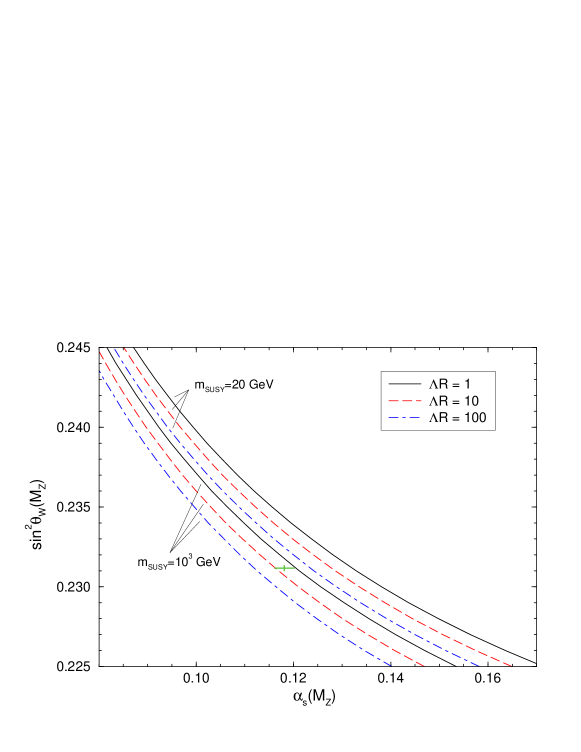
Figure 2: $\alpha_{s}(M_{Z})$ as a function of $\sin^{2}\theta_{W}(M_{Z})$ varying $m_{\scriptscriptstyle SUSY}$ in the range $20-10^{3}$ GeV for $\Lambda R=1,10,100$. The experimental point is shown in green.

Increasing the value of $\Lambda R$, the curve goes in the right direction, approaching the experimental values $\alpha_{s}(M_{Z})=0.1181\pm 0.002$, $\sin^{2}\theta_{W}(M_{Z})=0.23117\pm 0.00016$ ($\overline{\text{MS}}$ scheme) [25]. Similar considerations apply to the plot in fig.(3) in which $\alpha_{s}(M_{Z})$ and the unification scale $1/R$ are extracted using the experimental value of $\sin^{2}\theta_{W}(M_{Z})$.

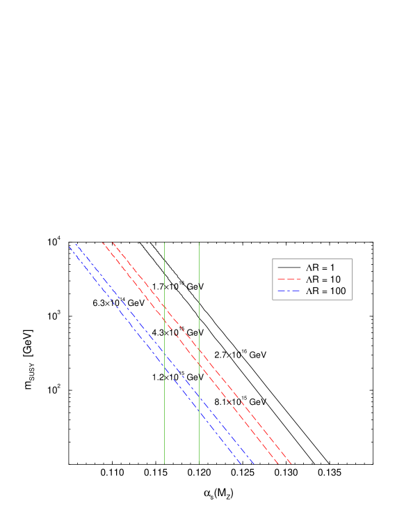
Figure 3: $\alpha_{s}(M_{Z})$ as a function of $m_{\scriptscriptstyle SUSY}$ for $\Lambda R=1,10,100$. The region between lines of the same style represents the uncertainty coming from the experimental error on $\sin^{2}\theta_{W}(M_{Z})$. The region between the green vertical lines is the measured value of $\alpha_{s}(M_{Z})$. The predicted values for $1/R$ are shown in the different regions.

Indeed for the preferred value $\Lambda R\sim 100$ the band of prediction (fig. 2) sits precisely on top of the measured values, with an interesting improvement over tree level matching. Unfortunately for this value of $\Lambda R$ one gets also $1/R\sim 10^{15}$ GeV, which is somewhat smaller that the lower bound from proton decay $1/R>5\times 10^{15}$ GeV [8]. Indeed for $\Lambda R>10$, the right value of $\alpha_{S}$ is obtained only for $1/R<5\times 10^{15}$ GeV. This is in agreement with what found in ref. [8]. While the strict NDA assumption does not work too well, we should be aware that we are talking about small effects: $\ln\Lambda R\sim 5$ is not a very big number and the $\Delta_{i}(\Lambda)$ may play role. In the end, we are forced to conclude that even though the running of boundary couplings gives an effect that goes in the right direction we still need the help of the almost comparable initial value $\Delta_{i}(\Lambda)$ to agree with the data and satisfy proton decay constraints.

6 Conclusions

We have applied the running and matching technique to study gauge unification with one extra compact dimension. We have used dimensional regularization for which power divergences are absent and which is therefore very convenient for doing effective field theory studies [12]. Moreover dimensional reduction is needed to consistently perform NLO calculations in supersymmetric theories. In orbifold models the radius dependence of the matching function is determined by the mismatch between the RG evolution of the low energy $1/g_{i}^{2}$ and the RG evolution of some gauge kinetic terms localized at the fixed points. The bulk gauge coupling does not run, so it is just a spectator in the matching. The main role in determining corrections to gauge unification is played by the boundary kinetic terms: these are free parameters and in general are not unified. Focusing on the $SU(5)$ model on $S_{1}/(Z_{2}\times Z_{2}^{\prime})$ of ref. [5, 8], we have discussed to what extent strong coupling assumptions based on NDA can control these unknown effects and lead to a more predictive set up. Our conclusion is that these models, when supplemented with NDA, stay more or less on the same level as usual GUTs, where threshold effects are controlled by assuming a non hierarchical GUT spectrum. Also in our case, in order to get a better agreement with the measured value of $\alpha_{s}$, one has to rely on small incalculable effects.

References

- [1] H. Georgi, S. Glashow, Phys. Rev. Lett. 32 (1974) 438.
- [2] for a NLO analysis see P. Langacker, N. Polonsky, Phys. Rev. D47 (1993) 4028 and references therein.
- [3] E. Witten, Nucl. Phys. B258 (1985) 75.
- [4] Y. Kawamura, Prog. Theor. Phys. 103 (2000) 613.
- [5] Y. Kawamura, Prog. Theor. Phys. 105 (2001) 999.
- [6] R. Barbieri, L. Hall and Y. Nomura, Phys. Rev. D63 (2001) 105007.
- [7] G. Altarelli, F. Feruglio, Phys. Lett. B511 (2001) 257.
- [8] L. Hall and Y. Nomura, hep-ph/0103125.
-
[9]
A. Hebecker and J. March-Russell, hep-ph/0106166;
R. Barbieri, L. Hall and Y. Nomura, hep-ph/0106190;
J. Bagger, F. Feruglio and F. Zwirner, hep-th/0107128;
A. Masiero, C.A. Scrucca, M. Serone and L. Silvestrini, hep-ph/0107201;
L. Hall, H. Murayama and Y. Nomura, hep-th/0107245;
L. Hall, Y. Nomura and D. Smith, hep-ph/0107331;
N. Haba et al., hep-ph/0108003;
I. Antoniadis, K. Benakli and M. Quiros, hep-th/0108005;
L. Hall, Y. Nomura, T. Okui and D. Smith, hep-ph/0108071. - [10] A. Hebecker and J. March-Russell, hep-ph/0107039.
- [11] R. Barbieri, L. Hall and Y. Nomura, hep-th/0107004.
- [12] S. Weinberg, Phys. Lett. B91 (1980) 51.
- [13] H. Georgi, A.K. Grant, G.Hailu, Phys. Lett. B506 (2001) 207.
- [14] R. Contino, L. Pilo, R. Rattazzi, A. Strumia, JHEP 0106 (2001) 005; hep-ph/0103104.
- [15] K. R. Dienes, E. Dudas and T. Gherghetta, Phys. Lett. B436, (1998) 55.
- [16] L. Hall, Nucl. Phys. B178 (1981) 75.
- [17] L. J. Dixon, V. Kaplunovsky and J. Louis, Nucl. Phys. B355 (1991) 649.
- [18] M. A. Shifman and A. I. Vainshtein, Nucl. Phys. B277 (1986) 456.
- [19] N. Arkani-Hamed and H. Murayama, JHEP 0006, (2000) 030; hep-th/9707133.
- [20] K. Konishi and K. Shyzuia, Nuovo Cim. A90 (1985) 111.
- [21] Z. Chacko, M. A. Luty and E. Ponton, JHEP 0007, (2000) 036; hep-ph/9909248.
- [22] R. Barbieri, L. Hall, Phys. Rev. Lett. 68 (1992) 752; see also J. Hisano, H. Murayama and T. Yanagida, Phys. Rev. Lett. 69 (1992) 1014.
- [23] M.B. Einhorn, D.R.T. Jones, Nucl. Phys. B196 (1982) 475.
- [24] M. Carena, S. Pokorski, C. Wagner, Nucl. Phys. B406 (1993) 59.
- [25] Review of Particle Physics, Particle Data Group, Euro. Phys. J. C15 (2000) 1.