On the structure of the virtual Compton amplitude
with additional final-state meson in the extended Bjorken region
Johannes Blümlein
johannes.bluemlein@desy.de Deutsches Elektronen-Synchrotron, DESY-Zeuthen,
Platanenallee 6, D-15735 Zeuthen, Germany
Jörg Eilers
eilers@itp.uni-leipzig.de Center for Theoretical Studies and Institute of
Theoretical Physics, Leipzig University, Augustusplatz 10,
D-04109 Leipzig, Germany
Bodo Geyer
geyer@itp.uni-leipzig.de Center for Theoretical Studies and Institute of
Theoretical Physics, Leipzig University, Augustusplatz 10,
D-04109 Leipzig, Germany
Dieter Robaschik
drobasch@physik.tu-cottbus.de BTU Cottbus, Fakultät 1, Postfach 101344,
D-03013 Cottbus, Germany
Abstract
Using the framework of the non-local light-cone expansion a
systematic study is performed for the structure of the twist-2
contributions to the virtual Compton amplitude in polarized
deep-inelastic non-forward scattering for general nucleon spin with an
additional scalar meson in the final state. A useful kinematic
parameterization allowing for appropriate triple-valued off-forward
parton distribution amplitudes is given. One-variable amplitudes being
adapted to the fixed parameters of the extended Bjorken region are
introduced by decomposing the Compton amplitude into collinear and
non-collinear components. These amplitudes obey Wandzura-Wilczek and
Callan-Gross like relations. The evolution equations for all the
distribution amplitudes are determined showing that the additional
meson momentum does not appear in the evolution kernels. The
generalization to outgoing mesons is given.
PACS: 24.85.+p, 13.88.+e, 11.30.Cp
Keywords: Twist decomposition,
Nonlocal light-cone operators,
Tensor harmonic polynomials,
Multivalued distribution amplitude,
Extended Bjorken region
I Introduction
Compton scattering of a virtual photon off a hadron,
(1.1)
is an important process in Quantum Chromodynamics. This general
process covers a series of different reactions through which a variety
of inclusive informations on the short–distance structure of nucleons
become accessible at large space–like virtualities. It is also
closely connected to the spin problem of the nucleon. The case of
forward scattering describes deep inelastic scattering
(DIS) off unpolarized or polarized targets which is widely discussed
in the literature, see e.g. DIS ; MUTA , and
corresponds to the generic (ordinary) non-forward virtual Compton
scattering MRGHD ; CS ; BGR97 ; BGR99 ; BR00 , for recent reviews
see REV1 . In the special case
, i.e., when the outgoing photon is real,
this process is called deeply virtual Compton scattering (DVCS).
Experimental results on polarized and unpolarized (deeply virtual) Compton
scattering were reported in EXP0 ; EXP1 ; EXP2 ; EXP3 ; EXP4 . The kinematic domain of some
of these investigations is bound to rather low values of .
Experimentally the final state in deep–inelastic non–forward
scattering contains aside the (virtual) photon and final–state
hadron, Eq. (1.1), a series of other hadrons, which even may emerge at
the amplitude–level. The latter process is much more likely
and of greater practical
importance than that
of a single isolated hadron
, which was studied
before MRGHD ; CS ; BGR97 ; BGR99 ; BR00 .
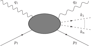
In this paper we extend the description given in the ordinary
non-forward case in Refs. BGR97 ; BGR99 ; BR00 to physical processes with an
outgoing scalar meson,
(1.2)
to investigate which of the properties derived in
Refs. BGR97 ; BGR99 ; BR00 remain valid in the more general
situation and which are changing to account for more realistic
experimental situations which allow for additional studies of
distribution functions emerging in non–forward scattering
111Similarly to the case of deep–inelastic non–forward
scattering multiple hadron final states also emerge in deep–inelastic
diffractive scattering EXPDIFFR along the diffractive final
state proton, which is assumed an isolated particle in the ideal case,
c.f. Ref. BR01 ..
If one looks for a diagrammatic representation of the amplitude for the
process (1.2) then even in the special kinematics
of the Bjorken region for being small, there appear
different production mechanisms.
However, if one has in mind
and then soft processes between the two final
particles and the incoming particle are essential and
we have to use a generalized distribution amplitude
. For other cases one may try to make models
which use wave functions of the nucleon and the meson
.
The Compton amplitude for the process (1.2) is given by
(1.3)
where
(1.4)
and are chosen as independent kinematic variables. As usual
and denote the four-momenta of the
incoming (outgoing) nucleons and photons, respectively. and
are the spins of these nucleons and is the momentum of the
outgoing scalar meson. denote the independent
kinematic variables in the ordinary non-forward case. In principle,
this set of kinematic variables can be extended to the case of
outgoing (scalar) mesons of momenta with
.
In ordinary non-forward Compton scattering the generalized
Bjorken region is defined by the conditions
(1.5)
keeping the variables
(1.6)
fixed. This definition has to be extended now by taking into account
the additional momentum . We define the extended Bjorken
region for light-cone dominated QCD processes by the conditions
(1.5) keeping the following three variables
(1.7)
fixed. This can be extended furthermore to the case of mesons by
the obvious generalization of and keeping
fixed. In the limit , these
definitions reduce to the usual generalized Bjorken region.
For completeness, we list the different kinematic domains for
forward and general non-forward processes and the related scaling
variables. These domains are distinguished as follows:
•
Bjorken region for forward scattering; fixed quantity:
(or )
•
Generalized Bjorken region for ordinary non-forward
scattering, including DVCS kinematics for ; fixed
quantities: and . In the special case of DVCS
holds.
•
Extended Bjorken region for non-forward scattering with a
single outgoing scalar meson; fixed quantities: and
.
•
-Extended Bjorken region for non-forward scattering
with outgoing scalar mesons; fixed quantities: and
.
By conservation of momentum,
(1.8)
one can show that and possess the same interpretation
as in the ordinary non-forward case. Especially, also the relation
holds for processes including the
outgoing mesons. The variables describe the momentum
fractions of the mesons in the infinite momentum frame defined
by the momentum . In the following we restrict the consideration
to the case of one additional final-state meson and return to the case
of -mesons in Section VII.
It is important to remark that all physical processes mentioned
above are distinguished only by taking different matrix elements of
the same renormalized operator 222As has been shown
recently in Ref. BR01 , also the case of deep inelastic diffractive
scattering can be described following similar lines., namely the
renormalized () time-ordered () product
(1.9)
where denotes the
hadronic current and is the renormalized matrix. Near the
light-cone, this operator will be decomposed via the
non-local operator product expansion AZ78 into a series of
non-local light-ray operators and the corresponding coefficient
functions :
(1.10)
The coefficient functions are singular on the light-cone. They are
entire analytic functions with respect to resulting in
a restricted integration range . The
unrenormalized light-ray operators in this expansion are given by
(1.11)
with some specified -structure of Dirac matrices and the
usual path-ordered phase factor,
(1.12)
ensuring gauge invariance. Here is the gluon field, the
strong coupling constant and is a light-like vector depending on
via a non-null subsidiary four-vector ,
(1.13)
In Eq. (1.10) the flavor structure has been suppressed.
Eventually, in the singlet case, also operators containing the gluon
field strength and their dual
have to be taken into account. The contributions which contain four or
more (anti)quark fields will be denoted by ‘higher order terms’,
possibly also together with (powers of) the gluon field strength, etc.
By construction, the non-local light-cone expansion, depending on the
order of terms being taken into account, leads to a
(sub)asymptotically relevant part and a well-defined remainder being
less singular, see Ref. MUTA .
Taking matrix elements of the operators and performing a
Fourier transformation in the expression (1.3) leads to
the physically interesting non-perturbative distribution amplitudes.
Because the operational input (1.9) for these amplitudes
is the same for the different processes described above, the evolution
equations of these amplitudes are determined by the renormalization
group equations of the operators and, therefore, also by
the same anomalous dimensions.
This paper is organized as follows. In Section II we discuss
the quark-antiquark operator (2.13) as operational input
for the (extended) Compton amplitude. This allows one to use the known
anomalous dimensions of this operator to
write down the evolution equations for the relevant distribution
amplitudes used in the process including an outgoing meson. The
evolution kernel required for these evolution equations is determined
by the anomalous dimensions of the quark-antiquark operator and
further computations of Feynman diagrams are not necessary, at least
at one–loop order. Furthermore this operator possesses a known twist
decomposition given in Refs. GLR99 ; GLR01 . In this paper we only
determine the twist-2 part of the Compton amplitude in the simply
extended Bjorken region which generalizes the twist-2
representation known for forward and ordinary non-forward scattering.
In Section III the twist decomposition of the matrix elements
and the necessary decomposition into suitable kinematic factors is
performed thereby using the hadron equations of motion. This section
also includes the definition of the distribution amplitudes used in
the process considered.
In Section IV the twist-2 part of the Compton amplitude is
calculated. It will be shown that, in the extended kinematic region,
the amplitude depends on the three scaling variables and
and is given by triple-valued distributions.
In Section V we extract integral relations
contained in the Compton amplitude and Section VI includes the
evolution equations obeyed by the distribution amplitudes.
In Section VII we add some remarks on generic properties of the
results obtained in the preceding sections and consider the case of
outgoing mesons; Section VIII contains the conclusions.
Appendix A contains the projections of the twist–2 operators on the
light cone. In the Appendix B we construct the
helicity basis for both photons and calculate all the helicity
amplitudes. These projections show in explicit form that the process
(1.2) is current conserving on the level of the
–matrix.
II Operator Structure
In this section we discuss the operator structure of the Compton
amplitude which will be used in the following sections. For brevity we
discuss only the flavor non-singlet case and drop all flavor
structures in the operators. The construction for the flavor singlet
case is to be carried out similarly.
As was mentioned above, the operator input for the Compton amplitude
is given by the renormalized time-ordered
product of two electromagnetic currents, Eq. (1.9).
Obviously, in lowest order in the coupling constant the -matrix can
be set equal to one. Then, applying the Wick-Theorem to this
time-ordered product and approximating the quark propagator near the
light-cone by
one obtains the following description of the operator
:
The renormalization symbol is suppressed in the notation. The
four-quark operator
has no singular
coefficient on the light-cone and is of minimal twist-4 and the last
term stems from disconnected diagrams. Both terms are therefore
discarded, see Ref. MUTA .
The quark mass terms resulting from the mass
dependent part of the operator are less
singular and will also be omitted. In fact, the lowest twist contribution
of all quark mass terms is contained in the operator
(2.3)
with and is of
twist-3.
The first term of the expansion (II) is of main
importance, because it contains the leading light-cone singularity and
its minimal twist contribution is of twist-2. It also contains terms
of higher twist (trace terms) and quark mass terms resulting
from the mass dependence of the scalar propagator .
These terms are also less singular on the light-cone.
Using the standard relations
(2.4)
where we indicate that is symmetric in
and , and noticing that the operator
(II) is dominated by the light-cone singularity,
, one arrives at
(2.6)
with the (unrenormalized) light-cone operators
(2.7)
(2.8)
This expansion has to be viewed as a simple form of the non-local
light-cone expansion (1.10) from which the suitable
-structures can be read off. Considering general gauges also
the phase factors must be included
into the light-cone operators and . Taking
into account also higher order terms of the -matrix additional
operator structures come into the play which, of course, are
sub-leading.
The -integration appearing in the light-cone expansion
(1.10) connects the coefficient functions, given here at Born
level,
(2.9)
with the respective operators. As is known from the general analysis
of the light-cone expansion MRGHD the Fourier transforms of the
coefficient functions in Eq. (1.10) are entire analytic
functions with respect to the variables which leads to a
restriction of the integration range of and to
the interval .
For later convenience we introduce the variables
(2.10)
and use the following integration measure in the light-cone
expansion
In terms of the variables and the coefficient
functions read:
(2.11)
Using these conventions one obtains the following representation of
the operator :
(2.12)
In general, the renormalized non-local operators
and
containing the phase
factors are given by
(2.13)
(2.14)
In the following we assume that the operators and
are renormalized quantities.
III Twist decomposition and matrix elements
The non-local operators and
, Eqs. (2.13) and
(2.14), contain contributions of different twist. Here, the
notion of twist is used in its original form GT71 as
(3.1)
The operators appearing in the expansion (2.12) of the
Compton amplitude have to be decomposed into their various twist
parts. On the light-cone they contain contributions of twist-2, 3 and
4
(3.2)
(3.3)
however, off the light-cone they contain an infinite series of
growing twist.
A group theoretical procedure of the twist decomposition has been
worked out in Refs. GLR99 ; GL00a and applied to various
physically relevant light-ray operators. As a result, the twist-2 part
of the operators (2.13) and (2.14) can be
constructed out of the twist-2 (pseudo) scalar operators
by applying the interior derivative
(3.4)
on the un-decomposed light-cone operators and performing a
subsequent integration (which stems from the normalization of
the local operators):
According to its structure the tracelessness of the operator
(III) which corresponds on the light-cone to the requirement
, is
trivially fulfilled due to the property of . An analogous
relation holds for the axial vector and pseudo scalar operator. The
twist-3 and twist-4 parts, however, cannot be constructed out of the
(pseudo) scalar operator since the latter, when restricted to the
light-cone, is already of twist-2.
Since we want to extract the twist-2 part of the Compton amplitude,
relation (III) will be applied to the matrix elements of the
operators considered :
(3.6)
Here, the spins of the nucleons have been suppressed in the
notation. Let us mention that the geometric twist decomposition of the
matrix elements is due to the twist decomposition of the non-local
operators. Usually, in phenomenological considerations another notion
of twist, called ‘dynamical’ twist, is considered which has been
introduced in the decomposition of the (forward) matrix elements by
Jaffe and Ji JJ91 . The interrelation of geometric and dynamic
twist was considered in Ref. GL01 . In the case of lowest
twist-2 there appears no difference, but for higher twist the mismatch
of dynamical twist with respect to geometric twist leads to differing
structures.
Because of translation invariance,
(3.7)
it is more convenient to discuss the centered operator
. Henceforth, for brevity,
will be denoted by .
In the ordinary non-forward case one usually parameterizes the
scalar matrix element by a Dirac- and a Pauli-type
contribution,
(3.8)
(3.9)
where and are on-shell spinors of the
incoming and outgoing nucleons, is a dimensional mass scale
which is kept fixed, and
. Because of
the Pauli type factor vanishes in the forward
limit. Using these kinematic factors the matrix element can be
parameterized as follows:
(3.10)
Here, the coefficient functions are the distribution
amplitudes in space. They depend on and all
possible products of the two momenta,
, as well as on the
renormalization scale and the coupling constant .
If an outgoing meson is present in the process, which means that
one has to contruct the matrix elements
, the representation
(3.10) of the scalar matrix element must be modified because
of the presence of the additional momentum . Especially, further
kinematic structures occur. They can be determined in a
straightforward way by using the following parameterization of the
scalar matrix element:
(3.11)
with
(3.12)
It is an easy task to find the general structure of
allowed by the momenta
, the metric and the
Levi-Civita tensor , demanding
not to be a pseudo scalar.
Using the equations of motion for the hadronic momenta
and with denoting the nucleon mass,
(3.13)
(3.14)
the decomposition of the matrix element (3.11) is :
(3.15)
where an auxiliary mass has been introduced in order to get
kinematic structures of equal dimensionality. Then, the scalar matrix
element is parameterized by a sum over the five kinematic factors
as follows:
(3.16)
where
generically denotes the multi-vector in the space of all the (three)
hadronic momenta.
Although one possible set of kinematic factors is given by
(3.16), it will be more convenient to choose another one
which is also linearly independent and contains the original kinematic
factors . Mimicking the Dirac- and Pauli-structures we choose
(3.17)
for the matrix element of the scalar operator and
(3.18)
for the matrix element of the pseudo scalar operator. For explicit
calculations it is important to note that each factor
has a linear -dependence,
Using the equations of motion again, the factors equal the
following combinations of
(3.19)
This shows that the constitute a suitable set of kinematic
factors for the scalar matrix element. In the limit they
obviously reduce to the Dirac- and Pauli-structures. Analogous
statements hold for .
The decomposition of the matrix element of
and
now reads
(3.20)
(3.21)
In principle there is also a dependence on variables like
. Because the latter dependence
vanishes on the light-cone, it will not be discussed in the further
considerations. As has been shown in Ref. GLR01 the whole
dependence is governed by harmonic extension off the light-cone
if the operator structure is already given on–cone. The
dependence is governed by the evolution equations obeyed by
the functions and will be discussed in Section VI.
As next step, a Fourier transformation of the functions
is performed,
(3.22)
Because also the functions
are entire analytic in the variables , the
support of their Fourier transforms is
restricted to the interval in the variables
. Therefore, the measure
(3.23)
has been introduced to realize this support.
is simply the product of the vectors
and , see (III). To get a
representation in the momenta and one introduces the
variables
with
Using the abbreviation
the scalar matrix element is represented by
(3.25)
In the following the explicit summation over will be omitted,
but will be indicated by the position of the index .
The expression (3.25) will be inserted into
(3.6) to calculate the matrix element of .
Thereby, it is important to state that the scaling in equation
(3.6) refers to and not to . Performing a
change of variables and
we get the following form of the matrix element, for the general case
:
where the abbreviation
(3.27)
has been used. Carrying out the differentiations we get
This form of the matrix element is yet rather complicated. Since
only the centered operator is needed in the following considerations,
we set .
To derive a simpler representation for the matrix element, the
-integration will now be comprised into the functions and
, the latter denoting the trace part, defined by
(3.29)
(3.30)
with given by
(3.31)
Obviously, these distribution amplitudes are not independent, and
the restricted integration range in space finally is contained in
the support properties of the distribution amplitudes
and .
After the substitution of and in
(III) with one obtains
(3.32)
for the matrix element of the twist-2 part of the vector operator
. The matrix element of the axial vector operator
possesses a similar representation
(3.33)
with and defined analogously to
and , by exchanging and in
(3.29) and (3.30).
Here, some general remarks are in order. First, the triple-valued distribution amplitudes
and are uniquely related to
the twist-2 (axial) vector operators and, in principle, should have
been marked by the related twist . However, since we do not
consider higher twist this has been omitted. Second, every
distribution amplitude of definite twist – also off the light-cone –
depends only on the variables and, possibly, on the
momenta . The dependence is completely contained in the
accompanying factors including, of course, the exponential
. These general expressions which are
given in terms of Bessel functions of the argument
have been determined in
Ref. GLR01
(For the twist–2 case of DIS this statement has already
been made in Ref. BB91 .)
Restricting onto the light-cone leads to the
expressions (3.32) and (3.33).
Third, these properties
hold for the operators of definite twist and are transposed to the
corresponding matrix elements, independently how many particles
(momenta) occur in the incoming and outgoing states. Therefore, if a
Fourier transformation containing these matrix elements has to be
performed this can be done by simply replacing . (In
Appendix A we give these expressions explicitly together with their
restriction onto the light-cone.) This will be applied in the next
Section for the expressions Eqs. (3.32) and
(3.33).
IV Compton amplitude
Now, we are in a position to compute the twist-2 part of the Compton
amplitude (1.3). Of course, we need it in the extended
Bjorken region and, therefore, can restrict our consideration to the
neighborhood of the light-cone. Thus, we will take the matrix elements
(3.32) and (3.33) with replaced by .
Merging everything together, we use the representation (2.12)
for the time-ordered product of two hadronic currents, insert
(3.32) and (3.33) for the matrix elements of
and and obtain:
The arguments and of the coefficient functions
are fixed at and
, so that we can use the symmetry properties of the
operators and ,
(4.2)
For the computation of the Compton amplitude it suffices to know the
operators at these given points, but for the investigation of the
evolution of the matrix elements their representation at general
values of and is needed, see Section VI for
the details.
Performing the -integration one obtains
(4.3)
where the abbreviation
(4.4)
has been used. The -term which results from the traces of
the twist-2 operator vanishes for the axial matrix element because
is symmetric. As a last step in the computation of
the Compton amplitude the Fourier transformation is carried out by
using
and the summation over and is performed in the
symmetric part of by using the form (II) for
. Then for the Compton amplitude we get
the result
which is expanded with respect to the functions , and
with the trace term separated from the antisymmetric
and remaining symmetric part.
This structure of the Compton amplitude is a generic one because it
is also valid for the ordinary non-forward case: The additional
structures arising due to the momentum are hidden in the summation
over the structure functions , and and
in the definitions of and . The reason for that result is
an outcome of the twist structure of the operator which is the same
for all the matrix elements under consideration. It holds also for the
case of outgoing mesons.
For and summation over the Dirac- and
Pauli-structures one reproduces the form of the Compton amplitude
given in Ref. BR00 . Here, the additional terms containing the
functions arise, because the trace term in
(3.6) has been taken into account. If is not present in
the process this term vanishes in the limit
(4.6)
(4.7)
(4.8)
setting and to zero. Therefore these terms
have been omitted in Ref. BR00 . If the five kinematic factors
containing the momentum are present this is
a priori no longer the case since non-vanishing contractions like
appear. Therefore, this term has been taken into
full account here.
In general, terms containing the product do
not vanish in the massless limit, while terms containing ,
, are small compared to the large
invariants. This leads to the approximation
We apply these approximations to the Compton amplitude and get a
representation for its twist-2 part in the massless limit and in the
extended Bjorken region, which depends explicitly on the three
variables and :
This form of the Compton amplitude will be used in the further
considerations.
V Integral relations
The variables and are not directly measurable because
they appear as Fourier variables of the distribution amplitudes .
The scaling variable , however, can be regarded as a physical
quantity and it is therefore quite natural to use the new variable
(5.1)
as integration variable in the denominators of Eq. (IV).
By the definition (III) the vector contains the variables
and and must be rewritten using the set
. This is simply done by introducing the combinations
(5.2)
(5.3)
which leads to the representation
(5.4)
The 4–vectors and define off–collinear
directions w.r.t. to the direction ; vectors along this momentum
are denoted as collinear. Note that these vectors are non-forward
still, since . contains collinear and off-collinear
contributions, the former of which are associated with the scaling
variable only. It will turn out that these collinear parts play
the dominant role in the process considered.
Different powers of contained in (IV), of course,
will lead to a whole series of structure functions corresponding to
different moments in and . Therefore, let us generally
define double moments of the triple-valued distribution amplitudes
leading to single-valued distributions as follows:
(5.6)
with
(5.7)
In fact, the values occur in the antisymmetric part and
the values in the symmetric part. To keep the discussion
short, we consider the antisymmetric part of the Compton amplitude in
full detail and give the result for the symmetric part only for the
leading terms, i.e., suppressing the trace terms. The explicit
calculation shows that the latter terms do not contribute to the
leading order in .
Because the contractions are only present for
the Dirac structure, , we
discuss this term separately. Then, the antisymmetric part of
(IV) is given by
At this point it is necessary to perform a partial integration in
the second term proportional to using the formula
(5.9)
which leads to
Several tensor structures contribute. Note that in the foregoing
discussion no assumption has been made on the direction of the
nucleon spin. As the polarization of the initial state nucleons in
experiment is performed in outer magnetic fields, the direction of the
nucleon spin is not related to other vectors in the system except for
the condition to hold.
The form (V) of the polarized Compton amplitude is very
interesting because it includes a Wandzura-Wilczek (WW) like relation
between the distribution amplitudes being associated to two of the
tensor structures 333For special choices of the nucleon spin
vector, e.g. when directed along the momentum , the second tensor structure may
become identical to the former one up to sub–leading corrections of
as well–known from the case of forward scattering, see
e.g. Ref. BLTA . Although the second structure appears as
kinematically suppressed it is still present and a WW like relation between
the twist–2 contributions of the two amplitudes exists. For other
choices of the spin vector this suppression does not occur.. This
relation becomes obvious, once the definitions
(5.11)
(5.12)
(5.13)
(5.14)
are made. This leads to a very simple form of the antisymmetric part
of the Compton amplitude, namely,
All the above functions are expectation values of
twist–2 operators.
By definition and obey the following integral
relation
(5.15)
This relation between two twist–2 quantities
can be viewed as a generalization of the WW-relation known
from forward scattering WW77 ,444Needless to say that
the Lorentz decomposition of the complete Compton amplitude delivers
higher twist corrections to the quantities as well;
in some cases twist–3 terms are present in the massless limit.
These contributions are not dealt with in the present paper. We mention
that in the case when quark and target mass corrections are taken into
account all contributions may receive higher twist corrections starting
with twist–3, as has been shown for the forward
case in Ref. BLTA . Integral relation between higher twist
contributions do also exist..
It is a property of the collinear
part of the polarized Compton amplitude and
connected to the -moment in and . The off-collinear
vectors and are connected to the new parton
distributions and , which obey an integral
representation in terms of the functions and
respectively, similar to . However, unlike
the case for the respective functions do not appear in the
Compton amplitude. Therefore we obtain at the present level only one
Wandzura–Wilczek like relation between the twist–two parts of the
respective amplitudes. Of course all the functions do receive
higher twist contributions, which were not discussed in the present
paper. Also these contributions as emerging in the different
amplitudes may obey similar integral relations. The generalization
(5.15) of the WW-relation has been obtained in
Ref. BR00 for the ordinary non-forward process
(1.1) without outgoing meson. The foregoing discussion
shows that it remains valid for the more general process
(1.2).
The Wandzura–Wilczek relation Eq. (5.15) is an
identity between physical amplitudes which emerges at the level of
geometric twist–2 as a consequence of the fact that the
distribution appears two times in the
decomposition of the Compton amplitude. These relations which
determine the (geometric) twist-2 content of the dynamical twist-3
distributions have to be called geometric WW relationsBLKO ; BLTA ; BR00 ; BL01 ; L01a . They are obtained by using solely
group theoretical means lying behind the definition of (genuine)
geometric twist, Eq. (3.1). These WW-relations have to be
distinguished from the so-called dynamical WW-relations being
obtained by using the QCD equations of motion as has been done by
dWW . To bring it to the point:
Geometric WW relations are written
for distributions having equal geometric twist, whereas dynamic WW
relations are written between distributions of equal dynamic twist.
Despite having the same formal structure their physical content is
different. For a detailed discussion of these relations
in the case of meson wave functions see Ref. BL01
which, however, with appropriate modifications also
holds for general non-forward amplitudes
(See also Ref. GL00a where the case of quark distributions
is discussed).
We now return to the discussion of the term containing the
contractions . To begin with, we first remind
that only the Dirac structure is of relevance in this
case and one may use the approximation
(5.16)
in the limit of vanishing nucleon masses. Even more general, one can
state that the product is of order and
is of order with . The
additional terms are therefore of non-leading type, but are
interesting because these structures arise due to the meson momentum
.
Inserting the above approximation and performing again partial
integrations leads to the complete form of .
with
(5.18)
(5.19)
(5.20)
The meson momentum and the momentum transfer are connected
to similar structures, but the functions related to are
far more complicated than . However, despite that fact the
expressions within the parentheses in Eqs. (5.18) –
(5.20) could be written in the same manner as the expressions
(5.12) – (5.14) showing potential WW-like
expressions for the twist-2 distributions
.
For the symmetric part of the Compton
amplitude we perform the same calculational steps as in the
antisymmetric part, namely:
•
Separation of contractions; this also
includes the trace terms.
Partial integration with respect to by formula
(5.9).
•
Projection onto the collinear part.
After partial integration the symmetric part of the Compton
amplitude has the following form:
The collinear part of , which contains only
functions and , can be written as
Looking at the tensor structure of (V), the
functions
(5.23)
(5.24)
appear as natural structure functions and obey a Callan-Gross like
relation CG69 :
(5.25)
Similar to Ref. BR00 one observes that the remainder
contributions in Eq. (V) are suppressed for large
values of , a property of the off-collinear terms. One may see
this, contracting the structures with the
respective tensors in front. As well known from forward scattering,
the Callan–Gross relation receives corrections both from higher
orders in the coupling constant and due to mass effects, see
e.g. Ref. GP , and therefore as well in the non-forward case. On the
other hand, the Wandzura–Wilczek relation for geometric twist–2
turns out to be rigidly stable, see e.g. Ref. BLTA .
Including also -contractions in the
calculation will result in an additional tensor structure analogous to
(V) with replaced by in
Eq. (V). The corresponding structure functions will
not be given in explicit form.
VI Evolution equations for the distribution amplitudes
The scaling violations of the operator matrix elements and
distribution amplitudes of the process considered are described by the
renormalization group equations governing the ultra–violet behavior
of the light–cone operators. The corresponding equations for the
distribution amplitudes are called evolution
equations, which we are going to discuss in and space. Since
the flavor content of the operators (2.7) and
(2.8) has been suppressed in the preceding sections, we
treat only the flavor non-singlet evolution equations as an example.
The singlet evolution equations are of quite similar structure (see
e.g. Ref. BGR99 ; for earlier work see Refs. BGR87 ; BB89 ).
The non-singlet renormalization group equation for the twist-2
vector operator reads
(6.1)
By contraction with it is obvious that the scalar
twist-2 operator obeys exactly the
same renormalization group equation because multiplication with
commutes with the differentiation on the left and with the
integration on the right hand side. This gives the renormalization
group equation for the scalar operator which on the light cone already
is of twist-2:
(6.2)
In the last equations the integration measure
(6.3)
has been introduced. In Refs. BGR87 ; BGR99 it is shown that
the non-local anomalous dimension matrix is invariant under
translations and scale transformations,
which reduces the number of independent variables of by
two. By first changing the variables from to
, followed by a translation by and a scaling by
one derives the following form of the evolution kernel
:
with
(6.6)
The variables and are connected by the following
transformation
(6.7)
It is therefore more natural to use and as integration
variables in the renormalization group equation (6.2)
instead of and . The integration measures are
related by
(6.8)
where and include the suitable
-functions realizing the integration ranges of
(6.3) and :
The measure can be divided into two parts, because
under the exchange
obeys the following relations, cf.
Ref. BGR99 :
(6.9)
Putting (VI) and (6.8) into the renormalization
group equation for the scalar operator results in
(6.10)
For the explicit structure of
see Refs. BGR99 ; BGR87 ; BB89 .
The equation (6.10) will now be considered for the
matrix elements of the
scalar operator which are, according to equation (3.20),
given by
(6.11)
¿From this one obtains directly the evolution equation for the
distribution amplitudes in -space:
(6.12)
Because we are interested in evolution equations in -space, we
perform a Fourier transformation of equation (6.12). The
physically relevant transforms of are given by
(6.13)
Carrying out these transformations one arrives at the following
result:
Let us point to the remarkable fact that the variable
connected to the meson momentum only appears as a parameter in
and is not contained in the evolution kernel . The same
observation has been made in Ref. BR01 recently in the case of
diffractive scattering, where the parameters or behave
in the same way. In so far some of the scaling variables of a problem,
in the present case the variables , play another role than
others, as here and , which interfere with the evolution.
This evolution equation is a fundamental equation because it
describes the evolution of the triple-valued distribution amplitudes
in space. These amplitudes are the basic
objects for the construction of the structure functions
and in (3.29) and (3.30). They are also used
in the definition of the single-valued functions
in (V). The
scaling violations of these functions are obtained solving
Eq. (6.16) and inserting the functions into
Eqs. (3.29,3.30).
It is also possible to obtain another evolution equation for
in the variable , which is
compatible with the former equation. This single-variable evolution
equation governs the evolution of the structure functions contained in
the collinear part of the Compton amplitude.
To begin with, we first show that the distribution amplitude
given by
(6.17)
has another representation obtained as
(6.18)
The constraints
(6.19)
(6.20)
appearing in the former equation are the scaling relations
(1.7) in space. Using the representation
(3.25) under these constraints leads to the
result (6.17).
To derive the single-variable evolution equation we form matrix
elements of equation (6.10),
(6.21)
and perform the Fourier transformation in the variable
according to (6.18). The direct
calculation leads to
(6.22)
with the evolution kernel
(6.23)
Like the evolution kernel , also
does not depend on any dependent variables
like or being related to the meson momentum.
VII Generalization to an arbitrary number of outgoing mesons
In this section we summarize the generic properties of the results
obtained in the preceding sections and extend it to an arbitrary
number of outgoing mesons. Generally, one may state that all the above
results remain valid under slight modifications if two or more
outgoing scalar mesons are present in the process,
To fix the kinematic domain of this process, all meson momenta
are connected to different scaling variables defined by
(7.2)
where and are obviously given by
(7.3)
and and are introduced as in (1.7).
In order to compute the twist-2 part of the Compton amplitude
(7.4)
for the general process (7.1) one applies the
same approximations to the operator as in
Sections. II and III. Thus one uses the approximation
(2.12) and applies the twist-2 projection (III).
The technique used in Section III to construct the matrix
elements can be carried out for an
arbitrary number of scalar mesons where the additional meson
momenta enlarge the set of kinematic factors
. However, these factors are easy to guess
and their number is given by
(7.5)
for the scalar matrix element. This formula also reproduces the
number of kinematic factors in the ordinary non-forward case: the
Dirac- and Pauli-structures.
Having all kinematic factors at hand, one introduces the
related structure functions and writes down the following
decomposition of the scalar matrix element
With this representation one goes through the same steps of the
calculation as in the preceding sections, namely
•
Fourier transformation of
•
Application of the twist-2 projector
•
Computation of the Compton amplitude.
The result is again of the form (IV) with a larger
space and given by
(7.6)
In this sense, the form (IV) of the Compton amplitude
is a generic result holding for a large class of processes. The more
explicit form (IV) is generalized by replacing
by .
It is even possible to interpret the Wandzura–Wilczek and
Callan–Gross relations obtained in Section V as
generic properties of the collinear parts of these processes. Making
the substitution
(7.7)
and projecting onto the collinear part one finds again the relations
(7.8)
(7.9)
Looking at the derivation of the evolution equation in
Section VI, it is not difficult to find the appropriate
generalization to an arbitrary number of mesons
():
(7.10)
For , this general evolution equation is reproducing the flavor
non-singlet part of the evolution equation given in Ref. BGR99
for the ordinary non-forward scattering. As in the case of one meson
in Section VI the variables connected to the meson
momenta only appear as parameters and do not contribute to the
evolution kernel,
(7.11)
Only the number of mesons is relevant for the structure of this
kernel. The single-variable evolution equation is of the same form as
in the preceding section. One only has to enlarge the number of
scaling parameters .
(7.12)
VIII Conclusions
We studied the structure of the virtual Compton amplitude for
deep-inelastic non-forward scattering
at the level of the twist–2 contributions in lowest order in QCD in
the massless limit. In the extended Bjorken region, i.e.,
with and
kept fixed, the twist-2 contributions to the Compton
amplitude were calculated using the non-local operator product
expansion for general spin states. In this approximation the Compton
amplitude consists of five kinematically independent parts which in
the limit reduce to the well known Dirac- and Pauli-type
amplitudes. A decomposition of the Compton amplitude was performed
with respect to the helicity states of both (virtual) photons. In
complete analogy the (electromagnetic) gauge invariance of the
non-local light-cone expansion holds at the level of the –matrix
since the fact that the leptonic currents are conserved. Due to this,
only those contributions in the Compton amplitude are projected out,
which obey gauge invariance. Integral relations generalizing the
Callan-Gross and Wandzura-Wilczek relations for unpolarized and
polarized forward-scattering are derived by reduction to the collinear
parts of the Compton amplitude and, thereby, reducing the
triple-valued distribution amplitudes to one-valued ones (for
and fixed). In this connection
attention has been drawn to the difference between geometric and
dynamic WW-relations being related to different notions of twist. The
evolution kernels of these distribution amplitudes are obtained from
the (well-known) non-local anomalous dimensions of the (scalar)
twist-2 light-ray operators and
; they are independent of the
meson momentum . These results show that deeply virtual Compton
scattering off nucleons in the case of additional meson production
behaves quite similar to the case where mesons are absent. Both the
basic structural relations as well as the scaling violations are the
same in both cases. However, the structure of the Compton amplitude is
different in general, however only with corrections of
or less.
Acknowledgements.
The authors are grateful to M. Lazar and M. Diehl for various useful
discussions. In addition, J. Eilers gratefully acknowledges the Graduate
College ”Quantum field theory” at Center for Theoretical Studies of
Leipzig University for financial support.
Appendix A Projection of the twist-2 operator onto the light-cone
This appendix is devoted to the derivation of the results
(3.32) and (3.33) from the off–cone twist-2
non-local quark-antiquark operators obtained in Ref. GLR01 .
As has been shown there the nonlocal quark-antiquark operator of
geometric twist-2 has the following structure
:
(8.1)
Its th moment is given by
(8.2)
Here, for notational simplicity we used the following abbreviations:
(8.3)
(8.4)
The relation between the non-local and the local operators,
Eqs. (8.1) and (A), off the light-cone is obtained by
observing that the Bessel functions are generating functions of the
Gegenbauer polynomials (see, e.g., Ref. PBM , Eq. II.5.13.1.3):
(8.5)
where
is the Pochhammer symbol.
The projection onto the light-cone is obtained most easily by first
considering the local operators. Because of the series expansion of
the Gegenbauer polynomials (see, e.g., Ref. PBM , Appendix
II.11),
(8.6)
one observes that from the expression (8.4) on the
light-cone, , only the term with the highest power, i.e., for
, survives:
(8.7)
Using these results in the expression (A) we obtain:
(8.8)
Now, using
(8.9)
we are able to re-sum over according to
(8.10)
There are two options of doing this. In the first instance we may
replace in Eq. (A) by the derivative
acting on the exponential .
This way one retains the expression (III) of the non-local
twist-2 operator on the light-cone from which the expression
(3.32) has been derived. On the other hand, after taking
matrix elements of (8.1) and observing the definitions
(3.29) and (3.30) of the distribution amplitudes
and , one obtains
exactly the expression (3.32). Analogous results hold for
the axial vector case (3.33).
The same result could have been obtained also using the Poisson
integral for the Bessel functions (cf., Ref. BE ,
Eq. II.7.12.7),
(8.11)
for , in order to
express the functions (8.3) on the light-cone by
(8.12)
Then, after shifting the homogeneous derivations in the
expression (8.1) to the right and interpreting it as
acting on the exponential, some partial
integrations with respect to can be performed which,
finally, lead again to the expression (III) and
(3.32), respectively.
Appendix B Helicity projections and current conservation
In this appendix we construct the helicity projections of the
Compton amplitude generalizing the results of Ref. BR00 to the
present case. We start with the construction of the helicity basis of
the two virtual photons and . To simplify
this construction, we choose the Breit frame, in which the relevant
momenta read:
(9.1)
(9.2)
(9.3)
(9.4)
where is introduced as a mass scale of the hadronic momentum
with . To define the helicity basis we introduce
the two reference vectors
(9.5)
(9.6)
The polarization vectors of the photons and
are then given by
(9.7)
(9.8)
(9.9)
(9.10)
(9.11)
(9.12)
(9.13)
The normalization factors are given by
(9.14)
(9.15)
(9.16)
(9.17)
(9.18)
(9.19)
which follows from the relations
(9.20)
(9.21)
(9.22)
(9.23)
(see definitions (1.7) and note that
in the Breit frame) and conservation of momentum
(9.24)
(9.25)
The polarization vectors obey the following normalization condition,
(9.26)
with for and for . We now use this
helicity basis to compute all matrix elements
(9.27)
The result of the straightforward calculation is
(9.28)
(9.29)
(9.30)
(9.31)
(9.32)
(9.33)
for the symmetric part. The helicity projections of the trace terms
are all of order and therefore not given in explicit form. The
same calculation is is carried out for the antisymmetric part:
(9.34)
(9.35)
Here, we have only kept terms contributing to the highest power in
, because all other terms vanish in the limit .
Terms proportional to in the normalization factors have been
neglected, because they do not contribute to the highest power in
. The amplitudes and
are a priori not of order , because
is of order . But since the integrals
(9.36)
vanish, these amplitudes are also identical to zero.
In the above only the contractions of the helicity vectors with the
Compton amplitude were considered. For the physical process, however,
the corresponding projections for the leptonic tensors
have to be considered as well to see, which terms
contribute to the physical –matrix. Due to the fact that
(9.37)
holds all remaining terms in the projections and
are annihilated.
In leading order in only the amplitudes
and give a non-vanishing contribution in
the extended Bjorken region, whereas other terms for
are suppressed at least in . The explicit
calculation also shows that
(9.38)
in leading order. Only two of the sixteen amplitudes are relevant
for . Similar results have been obtained in
Ref. DGPR .
References
(1)
F.J. Yndurain, Quantum Chromodynamics. An Introduction to the
Theory of Quarks and Gluons, Springer, New York (1983),
F. Lenz, H. Grieshammer and D. Stoll (Eds.),
Lectures on QCD. II: Applications Springer, Berlin (1997).
(2)
T. Muta, Foundations of QCD. An Introduction to Perturbative
Methods in Gauge Theories, (World Scientific, Singapore, 1987).
(3)
D. Müller, D. Robaschik, B. Geyer, J. Horejsi, and F.-M. Dittes,
Fortschr. Phys. 42 (1994) 101, hep-th/9812448.
(4)
X. Ji, Phys. Rev. Lett. 78 (1997) 610; Phys. Rev. D55 (1997)
7114; J. Phys. G24 (1998) 1181;
A.V. Radyushkin, Phys. Lett. B385 (1996) 333; Phys. Rev. D56 (1997) 5524;
I.I. Balitsky and A.V. Radyushkin, Phys. Lett. B413 (1997) 114.
(5)
J. Blümlein, B. Geyer, and D. Robaschik, Phys. Lett. B406 (1997)
161.
(6)
J. Blümlein, B. Geyer, and D. Robaschik, Nucl. Phys. B560
(1999) 283.
(7)
J. Blümlein and D. Robaschik, Nucl. Phys. B581 (2000) 449.
(8)
M. Vanderhaeghen, Eur. Phys. J. A8 (2000) 455;
K. Goeke, M. Polyakov, and M. Vanderhaeghen, Progr. Part. Nucl. Phys.
47 (2001) 401.
(9)
P. Saull, for the ZEUS collaboration, hep-ex/0003030; Abstract
564, EPS HEP Budapest (2001).
(10)
C. Adloff et al.,
H1 collaboration, Phys. Lett. B517 (2001) 47.
(11)
A. Airapetian et al., HERMES collaboration, hep-ex/0106068.
(12)
MAMI collaboration, Nucl. Phys. A666 (2000) 44;
J. Roche et al., MAMI collaboration, Phys. Rev. Lett. 85 (2000) 708.
(13)
G. Audit et al., TJNAF experiment 93–050;
B.B. Wojtsekhovskii et al., TJNAF experiment 99–114;
J.P. Chen et al., TJNAF experiment 00–110.
(14)
J. Breitweg et al., ZEUS collabortaion, Eur. Phys. J. C6 (1999) 43;
C. Adloff et al., H1 collaboration, Z. Phys. C76 (1997) 613.
(15)
J. Blümlein and D. Robaschik, Phys. Lett. B517 (2001) 222.
(16)
S.A. Anikin and O.I. Zavialov, Ann. Phys. (N.Y.) 116 (1978) 135.
(17)
B. Geyer, M. Lazar, and D. Robaschik, Nucl. Phys. B559 (1999) 339.
(18)
B. Geyer, M. Lazar, and D. Robaschik, Power corrections of
off-forward quark distributions and harmonic operators with definite
geometric twist, hep-ph/0108061, Nucl. Phys. B in press.
(20)
B. Geyer and M. Lazar, Nucl. Phys. B581 (2000) 341.
(21)
R.L. Jaffe and X. Ji, Nucl. Phys. B375 (1991) 527.
(22)
B. Geyer and M. Lazar, Phys. Rev. D63 (2001) 094003.
(23)
I. Balitsky and V. Braun, Nucl. Phys. B361 (1991) 93.
(24)
J. Blümlein and A. Tkabladze, Nucl. Phys. B553 (1999) 427;
J. Phys. G25 (1999) 1553; Nucl. Phys. B (Proc. Suppl.)
79 (2000) 541.
(25)
S. Wandzura and F. Wilczek, Phys. Lett. B72 (1977) 195.
(26)
J. Blümlein and D. Kochelev, Phys. Lett. B381 (1996) 296
; Nucl. Phys. B498 (1997) 285.
(27)
P. Ball and M. Lazar, Phys. Lett. B515 (2001) 131-136.
(28)
M. Lazar, JHEP 0105:029 (2001).
(29)
A.V. Belitsky and D. Müller, Nucl. Phys. B589 (2000) 611;
N. Kivel, M.V. Polyakov, A. Schäfer, and O.V. Teryaev, Phys. Lett
B497 (2001) 73;
A.V. Radyushkin and C. Weiss, Phys. Rev. D63 (2001) 114012;
I.V. Anikin and O.V. Teryaev, Phys. Lett. B509 (2001) 95.
(30)
C.G. Callan and D.J. Gross, Phys. Rev. Lett. 22 (1969) 156.
(31)
H. Georgi and H.D. Politzer, Phys. Rev. D14 (1976) 1829.
(32)
Th. Braunschweig, B. Geyer, and D. Robaschik, Ann. Physik (Leipzig)
44 (1987) 407.
(33)
I. Balitsky and V. Braun, Nucl. Phys. B311 (1989) 541.
(34)
A.P. Prudnikov, Yu.A. Brychov, and O.I. Marichev,
Integrals and Series,
Vol. 2, Special Functions, Gordon and Breach Science Publishers,
New York.
(35)
H. Bateman and A. Erdelyi, Higher Transcendental Functions,
Vol. 2, New York 1953.
(36)
M. Diehl, T. Gousset, B. Pire, and J.P. Ralston, Phys. Lett. B411
(1997) 193.