EFFECTS OF SHADOWING ON DRELL–YAN DILEPTON PRODUCTION IN HIGH ENERGY NUCLEAR COLLISIONS


                      K.J. Eskola, V.J. Kolhinen, and P.V. Ruuskanen
                       Department of Physics, University of Jyväskylä P.O.Box 35, FIN-40351, Jyväskylä, Finland


                      R. L. Thews
                       Department of Physics, University of Arizona, Tucson, Arizona 85721, USA


Abstract

We compute cross sections for the Drell–Yan process in nuclear collisions at next-to-leading order (NLO) in $\alpha_{s}$. The effects of shadowing on the normalization and on the mass and rapidity dependence of these cross sections are presented. An estimate of higher order corrections is obtained from next-to-next-to-leading order (NNLO) calculation of the rapidity-integrated mass distribution. Variations in these predictions resulting from choices of parton distribution sets are discussed. Numerical results for mass distributions at NLO are presented for RHIC and LHC energies, using appropriate rapidity intervals. The shadowing factors in the dilepton mass range $2<M<10$ GeV are predicted to be substantial , typically 0.5 - 0.7 at LHC, 0.7 - 0.9 at RHIC, and approximately independent of the choice of parton distribution sets and the order of calculation.

Introduction

In a previous study [1] we provided a systematic survey of theoretical predictions for the Drell–Yan process [2, 3] in nucleon–nucleon collisions at energies relevant to ion–ion experiments at RHIC and LHC. In this study we extend our work to nuclear collisions at the same energies. A short theoretical discussion can be found in [1] and a more complete review of the perturbative QCD calculations in van Neerven’s article [3]. As before, we explore the uncertainties in the dependence of the production rate on the dilepton’s mass $M$ and rapidity $y$ due to the choice of parton distribution set. In addition, we investigate thoroughly the effects of nuclear shadowing [4] on the normalization and on the mass and rapidity dependence of these cross sections.

Our predictions for ${\rm d}\sigma^{AA}/{\rm d}M{\rm d}y$ are based on a perturbative analysis of the underlying partonic processes to order $\alpha_{\rm s}$ [5, 6, 7, 8]. The parton cross sections are folded with parton distributions which are extracted from data on the basis of next-to-leading order analysis. Unfortunately, only leading order determination of nuclear shadowing effects is available presently, partly due to the limited amount of data available for such a study. Even though it deserves a careful study, we feel that the main features of shadowing will not change qualitatively when going from leading order to next-to-leading order analysis.

As in earlier studies, we find that the perturbative corrections and the uncertainties due to the choice of parton set grow as $M$ decreases. From the point of view of the heavy ion physics, the mass region from 2 to 10 GeV is of most interest. In order to estimate the applicability of perturbative calculations at these relatively low mass values we recall results for the rapidity-integrated ${\rm d}\sigma/{\rm d}M$, for which the complete NNLO calculations (order $\alpha_{\rm s}^{2}$) are available. The relative magnitude of the NNLO correction sets one limit on our confidence in the applicability of perturbation theory. We show in Figure 1 the mass dependence of the $K$-factors from a calculation with NLO parton distributions and parton level cross sections up to NNLO. One sees that for $M>2$ GeV at RHIC energy and for $M>3.5$ GeV at LHC energy the NNLO contribution is at most about a 5 % correction to the NLO result. For lower masses at LHC energy the NNLO contribution grows sharply. At $M=2$ GeV, the NNLO correction alone is about 25 %, which is larger than the NLO correction itself of about 20 %. Hence in this mass and energy range we must consider the calculations as merely a general indication of magnitudes, since convergence of the QCD perturbative series is not yet evident. Keeping this caveat in mind, we restrict ourselves in the following calculations to the NLO results.

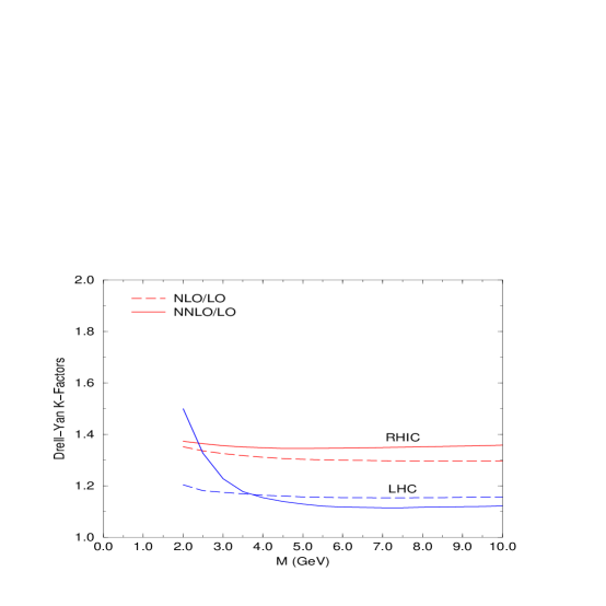
Figure 1: $K$-factors at RHIC energy (200 GeV) and LHC energy (5.5 TeV) for NLO (dashed lines) and NNLO (solid lines) Drell–Yan calculations of ${\rm d}\sigma/{\rm d}M$ using MRSG structure functions in proton-proton collisions.

We will not repeat here the discussion in [1] on the dependence of the cross sections on the renormalization scale $\mu_{\lower 2.0pt\hbox{$\scriptstyle{R}$}}$ and the factorization scale $\mu_{\lower 2.0pt\hbox{$\scriptstyle{F}$}}$, or choice of $\overline{\rm MS}$ or DIS regularization scheme. Since the determination of parton distributions has improved considerably during last few years, we calculate the NLO cross sections utilizing the recently-extracted CTEQ [9], GRV [10], and MRS [11] sets. In this connection we discuss also the dependence of the expected shadowing effects on the choice of parton distribution set.

In the next section we will define the average nucleon-nucleon cross section in a nucleus-nucleus collision and, using the nuclear transverse overlap function, the number distributions normalized to one collision. We will also briefly introduce the nuclear shadowing modifications to the parton distributions. In the following section we present the NLO results at RHIC and LHC energies. The effects of shadowing are then implemented, followed by numerical results on the rapidity-integrated cross sections. A discussion of general properties of the shadowing correction completes this work.

Cross sections and shadowing modifications

Let us consider a collision of two nuclei with mass numbers $A_{1}$ and $A_{2}$. Since the Drell–Yan process is sensitive to the isospin structure of the nuclei, we must specify also the proton numbers $Z_{1}$ and $Z_{2}$, and neutron numbers $N_{1}$ and $N_{2}$. We will assume that the shapes of the proton and neutron density distributions within a nucleus are the same:

$$\rho_{\lower 2.0pt\hbox{$\scriptstyle{\rm p}$}}({\bf r}) = \rho_{\lower 2.0pt\hbox{$\scriptstyle{\rm p}$}}(z,{\bf s})=\frac{Z}{A}\rho_{\lower 2.0pt\hbox{$\scriptstyle{A}$}}({\bf r}),$$

$$\rho_{\lower 2.0pt\hbox{$\scriptstyle{\rm n}$}}({\bf r}) = \rho_{\lower 2.0pt\hbox{$\scriptstyle{\rm n}$}}(z,{\bf s})=\frac{N}{A}\rho_{\lower 2.0pt\hbox{$\scriptstyle{A}$}}({\bf r}),$$ (1)

where $\rho_{\lower 2.0pt\hbox{$\scriptstyle{A}$}}({\bf r})$ is the total nucleon number density. In the numerical calculations we use the Wood-Saxon parametrization

$$\rho_{\lower 2.0pt\hbox{$\scriptstyle{A}$}}({\bf r})=\frac{n_{0}}{1+e^{(r-R_{\lower 2.0pt\hbox{$\scriptstyle{A}$}})/d}}$$ (2)

where $n_{0}=0.17\ {\rm fm}^{-3},\ d=0.54\ {\rm fm}$ and $R_{\lower 2.0pt\hbox{$\scriptstyle{A}$}}=1.12A^{1/3}-0.86A^{-1/3}\ {\rm fm}$. We define the nuclear thickness function $T_{\lower 2.0pt\hbox{$\scriptstyle{A_{i}}$}}({\bf s})$ and the overlap function $T_{\lower 2.0pt\hbox{$\scriptstyle{A_{1}A_{2}}$}}({\bf b})$ at impact parameter ${\bf b}$ as

$$T_{\lower 2.0pt\hbox{$\scriptstyle{A}$}}({\bf s}) = \int{\rm d}z\rho_{\lower 2.0pt\hbox{$\scriptstyle{A}$}}(z,{\bf s}),$$

$$T_{\lower 2.0pt\hbox{$\scriptstyle{A_{1}A_{2}}$}}({\bf b}) = \int{\rm d}{\bf s}T_{\lower 2.0pt\hbox{$\scriptstyle{A_{1}}$}}({\bf s})T_{\lower 2.0pt\hbox{$\scriptstyle{A_{2}}$}}({\bf b-s})\,.$$ (3)

In a $p-A$ collision we expect the total cross section of a hard process to be the sum of individual nucleon-nucleon cross sections,

$${\rm d}\sigma_{{\rm p}A}=Z{\rm d}\sigma_{\rm pp}+N{\rm d}\sigma_{\rm pn}.$$ (4)

The corresponding cross section ${\rm d}{\sigma}_{A_{1}A_{2}}$ for an $A_{1}+A_{2}$ collision can be written as

$${\rm d}\sigma_{A_{1}A_{2}}={Z_{1}}{Z_{2}}\,{\rm d}\sigma_{\rm pp}+{N_{1}}{Z_{2}}\,{\rm d}\sigma_{\rm np}+{Z_{1}}{N_{2}}\,{\rm d}\sigma_{\rm pn}+{N_{1}}{N_{2}}\,{\rm d}\sigma_{\rm nn}\,.$$ (5)

The average number distribution in one collision at impact parameter ${\bf b}$ is obtained by multiplying the average nucleon-nucleon cross section in $A_{1}+A_{2}$ collision, ${\rm d}{\sigma}_{A_{1}A_{2}}^{\rm NN}={\rm d}{\sigma}_{A_{1}A_{2}}/A_{1}A_{2}$, with the overlap function $T_{A_{1}A_{2}}({\bf b})$. In particular, for the mass distribution per unit rapidity in central, zero impact parameter collision we have

$$\frac{{\rm d}N_{\lower 2.0pt\hbox{$\scriptstyle{A_{1}A_{2}}$}}}{{\rm d}y{\rm d}M}=\frac{T_{\lower 2.0pt\hbox{$\scriptstyle{A_{1}A_{2}}$}}(0)}{A_{1}A_{2}}\,\frac{{\rm d}{\sigma}_{A_{1}A_{2}}}{{\rm d}y{\rm d}M}$$ (6)

In the QCD-based parton model the Drell–Yan cross section for nucleon($n_{1}$)-nucleon($n_{2}$) collision ($n_{i}={\rm p,n}$) can be expressed as

$${\rm d}{\sigma}_{\!n_{1}\!n_{2}}=\sum_{i,j}f_{i}^{n_{1}}(x_{1},\mu^{2})\otimes f_{j}^{n_{2}}(x_{2},\mu^{2})\otimes{\rm d}\hat{\sigma}_{\lower 2.0pt\hbox{$\scriptstyle{ij}$}}$$ (7)

in terms of partonic cross sections (or coefficient functions) ${\rm d}\hat{\sigma}_{\lower 2.0pt\hbox{$\scriptstyle{ij}$}}$ for partons $i$ and $j$ and parton distribution functions $f_{i}^{n_{1}}(x,\mu^{2})$ of parton $i$ in nucleon $n_{1}$. In numerical calculations it is practical to combine eqs. (5) and (7) to join the parton distributions in proton and neutron using appropriate weights to a parton distribution in an average nucleon.

The distribution of a parton flavour $i$ in a bound proton of a nucleus $A$ can be written as $f_{i/A}^{p}(x,Q^{2})=R_{i}^{A}(x,Q^{2})f_{i}^{p}(x,Q^{2})$, where $f_{i}^{p}(x,Q^{2})$ is the corresponding parton distribution of the free proton, and $R_{i}^{A}(x,Q^{2})$ defines the nuclear effects (shadowing) at each $x$ and $Q^{2}$. The parton distributions of bound neutrons can then be obtained by approximating $f_{u(\bar{u})/A}^{n}\approx f_{d(\bar{d})/A}^{p}$ and $f_{d(\bar{d})/A}^{n}\approx f_{u(\bar{u})/A}^{p}$ (exact for isoscalar nuclei) and $f_{i/A}^{n}=f_{i/A}^{p}$ for the isospin symmetric distributions.

In practice, we include the nuclear effects in the computation of the Drell–Yan dilepton cross sections ${\rm d}{\sigma}_{A_{1}A_{2}}^{\rm NN}$ by using the EKS98-parametrization of $R_{i}^{A}(x,Q^{2})$ [12]. EKS98 is based on the DGLAP analysis of Ref. [13] where the nuclear parton distributions are assumed to be factorizable above $Q_{0}=1.5$ GeV. The existence of nuclear effects at this scale is taken as a given fact (i.e. the origin is not discussed) and the absolute nuclear parton distributions are evolved to the region $Q>Q_{0}$ by using the standard lowest order leading twist DGLAP equations. Constraints for $R_{i}^{A}(x,Q^{2})$ are given by the data on the ratios of structure functions $F_{2}^{A_{1}}/F_{2}^{A_{2}}$ from deep inelastic lepton-nucleus scatterings, by the data on Drell–Yan dilepton production in proton-nucleus collisions, and by conservation of baryon number and momentum. More detailed discussion of the the analysis [13] is found in [4].

In [12] it was shown that the ratios $R_{i}^{A}=f_{i/A}^{p}/f_{i}^{p}$ are within a few percent the same for different sets of LO parton distributions of the free proton. However, as the DGLAP analysis [13] was only performed in the LO, we have a slight inconsistency in the NLO computation of the cross sections here. The difference to the NLO DGLAP analysis of the nuclear parton distributions is nevertheless expected to be small in the ratios $R_{i}^{A}$.

Sensitivity to Parton Distribution Functions

Figure 2: NLO Drell–Yan rapidity distributions at $\sqrt{s}=200$ GeV in p-p collisions for various parton distribution functions.

To estimate the sensitivity of the Drell–Yan calculations to the choice of parton distribution function sets, we have utilized the most recent analyses of the three major groups (MRST99, CTEQ5, and GRV98), where we have used the default parameters in the cases that more than one option is available. For further comparison, we have also used the previous versions from these same groups (MRSG, CTEQ4, and GRV94).

Shown in Figure 2 are the NLO differential cross sections in center of mass rapidity for proton-proton collisions at $\sqrt{s}=200$ GeV at $M=2$ and $M=10$ GeV. It is evident that at $M=10$ GeV the $x$-values probed are sufficiently large such that all distribution function sets are constrained by data to very similar values. (Recall that at LO the partonic $x$-values $x_{1}$ and $x_{2}$ are fixed at $x_{1,2}={M\over\sqrt{s}}e^{\pm y}$.) On the contrary, at $M=2$ GeV parton distributions at the lower $x$-values are not sufficiently constrained by data, and variations of 20 - 40 % between sets are not uncommon. Calculations with intermediate masses reveal that this large uncertainty essentially disappears already when $M=4$ GeV, such that above this mass the variations are bounded typically by 10 %.

Corresponding results for $\sqrt{s}=5.5$ TeV are shown in Figure 3.

Figure 3: NLO Drell–Yan rapidity distributions at $\sqrt{s}=5.5$ TeV in p-p collisions for various parton distribution functions.

A similar pattern exists also at this energy, but with somewhat different magnitudes. At $M=2$ GeV, the variation is at least a factor of 2. (Note that the apparent discontinuity in slope for the CTEQ curves are due to an absolute cutoff below a minimum $x$-value of $10^{-5}$.) As one increases $M$ this uncertainly again decreases rapidly, reaching the 10-15 % level at $M=10$ GeV.

Shadowing effects in rapidity distributions

For the effects of shadowing at RHIC and LHC, we choose a representative parton distribution set, the MRST99. Shown in Figure 4 are Au-Au LO and NLO cross sections per nucleon at RHIC for $M=2$ GeV and $M=10$ GeV, both with and without shadowing. One sees that at smaller $M$ the effects of shadowing are quite large, and in much of the kinematic range the magnitude is similar to that of the NLO corrections.

Figure 4: Shadowing in LO and NLO Drell–Yan rapidity distributions calculated with MRST99 structure functions for Au-Au collisions at RHIC with $\sqrt{s}=200$A GeV.

Figure 5: Shadowing in LO and NLO Drell–Yan rapidity distributions calculated with MRST99 structure functions for Pb-Pb collisions at LHC with $\sqrt{s}=5.5$A TeV.

Figure 6: Ratio of Shadowing/No Shadowing in LO and NLO Drell–Yan cross sections ${\rm d}\sigma/{\rm d}M{\rm d}y$ as a function of rapidity for fixed values of $M$ at RHIC with $\sqrt{s}=200$A GeV.

Figure 7: Ratio of Shadowing/No Shadowing in LO and NLO Drell–Yan cross sections ${\rm d}\sigma/{\rm d}M{\rm d}y$ as a function of rapidity for fixed values of $M$ at LHC with $\sqrt{s}=5.5$A TeV.

Figure 5 presents the same calculations at LHC for Pb-Pb collisions. The magnitudes of the shadowing corrections are even larger here, due to the smaller target $x$-values probed at this energy and rapidity range.

We also show in Figures 7 and 7 the ratio of cross sections with and without shadowing corrections. The dashed lines for LO are determined entirely by the fixed $x_{1,2}$ -values and the corresponding quark and antiquark shadowing ratios $R_{i}^{A}(x,Q^{2}=M^{2})$ for each nucleus.

The solid lines for the NLO ratios are not identical to those for LO, but are seen to follow those curves quite closely. This behavior is somewhat unexpected, since the NLO subprocesses involve integrals over $x$-values significantly different than the $x_{1,2}$. It cannot be explained by simple magnitude arguments, since the NLO $K$-factors are substantial, and also involve gluon structure functions not present in the LO contribution. What is evidently happening is that the NLO integrals can be approximated by mean values of the integrand at effective $x$-values close to the $x_{1,2}$. In any event, it appears that one may be able to extract overall multiplicative shadowing factors which will be approximately independent of the order of perturbative QCD and the input structure functions.

Mass distributions

We now calculate the expected mass distributions of the NLO nucleus-nucleus cross sections at RHIC and LHC, integrated over rapidity intervals appropriate for acceptance of the detectors (1.1 - 1.6 at RHIC and 2.0 - 4.0 at LHC). The results for RHIC are shown in Figure 9 for the MRST99, CTEQ5, and GRV98 structure functions. Both shadowing and no shadowing calculations are presented. Although there is a considerable difference between results with different structure functions, especially at low mass, this uncertainty is less than the expected differences between shadowing and no shadowing. Also shown are the ratios of shadowing to no shadowing predictions for calculations using each of the three structure functions. As anticipated, this results in a universal shadowing curve, approximately independent of structure function. The shadowing curve at the bottom of the figure actually displays all three results - the differences are smaller than the width of the lines.

Corresponding results for LHC are shown in Figure 9. The patterns are very similar. At the lowest mass there is somewhat more dispersion due to choice of structure function, but we already know that in this region both the reliability of pQCD at NLO is quite weak and the parton distributions are less constrained. The shadowing ratios converge again to a universal curve.

For archival purposes, we present in Table 1 the calculated NLO nucleus-nucleus cross section values for all three choices of structure functions, both with and without shadowing. In addition, we list the corresponding p-Au (at RHIC) and p-Pb (at LHC) NLO cross sections for the same detector rapidity interval in both the proton and nucleus directions. (At ALICE we take into account the asymmetric beam energies, and assume that the rapidity interval in the nucleus direction is reached by interchanging the beam directions.)

Figure 8: Rapidity-Integrated $1.1<y<1.6$ NLO Drell–Yan Mass distributions for Au-Au collisions at RHIC with $\sqrt{s}=200$A GeV.

Figure 9: Rapidity-Integrated $2.0<y<4.0$ NLO Drell–Yan Mass distributions for Pb-Pb collisions at LHC with $\sqrt{s}=5.5$A TeV.

Conclusions

We have studied the production of Drell–Yan dileptons at energies and phase space regions appropriate for the BNL-RHIC and CERN-LHC heavy ion experiments. The NNLO calculations, available for ${\rm d}\sigma/{\rm d}M$, indicate that a perturbative calculation converges well for $M\,\,\raise 2.0pt\hbox{$>$}\hbox to0.0pt{\hss\lower 3.0pt\hbox{$\sim$}}\,\,4$ GeV, the NNLO correction being $\,\,\raise 2.0pt\hbox{$<$}\hbox to0.0pt{\hss\lower 3.0pt\hbox{$\sim$}}\,\,5$ %. At the LHC energy it becomes rapidly less reliable as $M$ approaches 2 GeV. Using a representative selection of most recent parton distribution sets, MRS991 [11], CTEQ5 [9], and GRV98 [10], we found that the differences between the sets lead to an uncertainty in the cross sections which at small masses, $M\simeq 2$ GeV, is typically 20 – 40 % at RHIC but around a factor of two at LHC. This reflects the lack of precision experimental constraints on parton distributions at small $x$. At RHIC the results from different sets converge as $M$ increases, but at LHC persist at the 10 – 15 % level even for $M=10$ GeV. We investigated the nuclear effects using the parton distribution functions for free nuclei modified with multiplicative shadowing functions determined from the available experimental information [12]. At RHIC energy, shadowing reduces the cross section at $M\simeq 2$ GeV by a universal (i.e. independent of structure function set or order or perturbative QCD) factor of $\sim 35$ %. This factor approaches $\sim 10$ % for $M\simeq 10$ GeV. At LHC the reduction for small masses is $\sim$ 55 % and more than 30 % even at $M=10$ GeV. In summary, these calculations are limited by uncertainties due to convergence of the perturbative series and parton distributions which become large at small values of $M/\sqrt{s}$. Thus they are generally not a problem for all of the RHIC results, but become severe at LHC for $M\,\,\raise 2.0pt\hbox{$<$}\hbox to0.0pt{\hss\lower 3.0pt\hbox{$\sim$}}\,\,4$ GeV. The overall effects of shadowing at RHIC energies are smaller in magnitude than those at LHC, but the change of the mass distribution shape due to shadowing is a larger effect at RHIC.

Rapidity-integrated Drell–Yan cross section $\displaystyle{M^{3}\frac{{\rm d}\sigma}{{\rm d}M}}$ [$\mu$b GeV²] $M$ [GeV] MRST99 CTEQ5 GRV98 MRST99 CTEQ5 GRV98 Shadow Shadow Shadow $\sqrt{s}=200$ GeV, $1.1<y<1.6$ for Au-Au at RHIC 2.0 251 207 271 166 139 178 3.0 264 243 279 196 181 206 4.0 257 246 269 203 196 212 5.0 243 236 253 200 196 208 6.0 225 222 234 190 189 197 7.0 207 206 216 177 178 185 8.0 189 189 197 164 165 171 9.0 172 172 179 150 152 157 10.0 155 156 162 137 138 143 $\sqrt{s}=5.5$ TeV, $2.0<y<4.0$ for Pb-Pb at LHC 2.0 3680 1890 3400 1790 954 1650 3.0 4640 3450 4510 2540 1930 2440 4.0 5190 4390 5080 3060 2630 2940 5.0 5550 4960 5380 3440 3120 3280 6.0 5700 5310 5530 3680 3470 3500 7.0 5760 5510 5590 3830 3700 3650 8.0 5820 5620 5590 3970 3870 3750 9.0 5740 5650 5560 4000 3970 3810 10.0 5720 5640 5510 4050 4030 3840 $\sqrt{s}=200$ GeV, $1.1<y<1.6$ for p-Au, Au-p at RHIC 2.0 1.32, 1.28 1.10, 1.05 1.44, 1.38 .937, 1.20 .781, .992 1.01, 1.28 3.0 1.42, 1.35 1.31, 1.23 1.50, 1.42 1.06, 1.33 .987, 1.22 1.12, 1.40 4.0 1.40, 1.31 1.34, 1.25 1.47, 1.37 1.09, 1.33 1.05, 1.27 1.14, 1.38 5.0 1.34, 1.24 1.31, 1.20 1.40, 1.29 1.08, 1.27 1.06, 1.23 1.12, 1.31 6.0 1.27, 1.15 1.25, 1.13 1.32, 1.19 1.04, 1.17 1.03, 1.16 1.08, 1.22 7.0 1.19, 1.05 1.18, 1.04 1.23, 1.09 .995, 1.08 .991, 1.07 1.03, 1.12 8.0 1.11, .960 1.10, .955 1.14, .999 .942, .979 .938, .976 .976, 1.02 9.0 1.02, .870 1.02, .869 1.06, .907 .881, .883 .881, .884 .914, .919 10.0 .942, .786 .940, .787 .974, .819 .822, .796 .821, .797 .850, .828 $\sqrt{s}=8.8$ TeV, $2.0<y<4.0$ for p-Pb, Pb-p at LHC 2.0 20.3, 20.1 10.0, 8.24 18.5, 19.6 12.5, 15.8 6.20, 6.75 11.4, 15.5 3.0 26.3, 26.6 19.6, 17.3 25.5, 26.8 16.8, 22.7 12.6, 15.1 16.3, 22.7 4.0 30.2, 30.9 25.9, 23.9 29.4, 30.8 19.9, 27.6 17.1, 21.7 19.3, 27.2 5.0 32.9, 33.9 30.1, 28.7 31.7, 33.0 22.1, 31.2 20.3, 26.8 21.2, 30.0 6.0 34.4, 35.4 32.8, 31.9 32.9, 34.2 23.5, 33.4 22.5, 30.4 22.4, 31.8 7.0 35.2, 36.1 34.6, 33.7 33.6, 34.9 24.4, 34.7 24.0, 32.7 23.2, 33.0 8.0 36.1, 36.8 35.7, 34.7 34.0, 35.1 25.4, 35.8 25.1, 34.0 23.7, 33.7 9.0 36.0, 36.4 36.4, 35.1 34.1, 35.1 25.6, 35.8 25.9, 34.8 24.1, 34.1 10.0 36.4, 36.4 36.8, 35.3 34.0, 35.0 26.0, 36.2 26.4, 35.3 24.2, 34.2

Table 1: NLO Drell–Yan Calculations for RHIC and LHC

References

- [1] S. Gavin, S. Gupta, R. Kauffman, P. V. Ruuskanen, D. K. Srivastava and R. L. Thews, Int. J. Mod. Phys. A10 (1995) 2961.
- [2] S.D. Drell and T.M. Yan, Phys. Rev. Lett. 25 (1970) 316.
- [3] W.L. van Neerven, Int. J. Mod. Phys. A10 (1995) 2921.
- [4] K.J. Eskola, H. Honkanen, V.J. Kolhinen, P.V. Ruuskanen and C.A. Salgado, this volume.
-
[5]
K. Kajantie, J. Lindfors and R. Raitio, Phys. Lett. 74B (1978) 384;
J. Kubar-Andre and F.E. Paige, Phys. Rev. D19 (1979) 221;
G. Altarelli, R.K. Ellis and G. Martinelli, Nucl. Phys. B157 (1979) 461;
J. Kubar, M. le Bellac, J.L. Munier and G. Plaut, Nucl. Phys. B175
(1980) 251; B. Humpert and W.L. van Neerven, Nucl. Phys. B184 (1981) 225. - [6] R. Hamberg, W.L. van Neerven and T. Matsuura, Nucl. Phys. B359 (1991) 343; W.L. van Neerven and E.B. Zijlstra, Nucl. Phys. B382 (1992) 11.
-
[7]
T. Matsuura and W.L. van Neerven, Z. Phys. C38 (1988) 623;
T. Matsuura, S.C. van der Marck and W.L. van Neerven, Nucl. Phys. B319 (1989) 570; Phys. Lett. 211B (1988) 171. - [8] P.J. Rijken and W.L. van Neerven, Phys. Rev. D51 (1995) 44.
- [9] H. L. Lai, J. Huston, S. Kuhlmann, J. Morfin, F. Olness, J. F. Owens, J. Pumplin and W. K. Tung (CTEQ Collaboration), Eur. Phys. J. C12 (2000) 375-392 [hep-ph/9903282].
- [10] M. Glück, E. Reya and A. Vogt, Eur. Phys. J. C5 (1998) 461-470 [hep-ph/9806404].
- [11] A.D. Martin, W.J. Stirling, R.G. Roberts and R.S. Thorne, Eur. Phys. J. C4 (1998) 463; [hep-ph/9907231].
- [12] K.J. Eskola, V.J. Kolhinen and C.A. Salgado, Eur. Phys. J. C9 (1999) 61-68 [hep-ph/9807297]; http://www.phys.jyu.fi/research/urhic/eks98param.html; H. Plothow-Besch, ’PDFLIB: Proton, Pion and Photon Parton Density Functions, Parton Density Functions of Nucleus, and Calculations’, User’s Manual – Version 8.04, W5051 PDFLIB 2000.04.17 CERN–ETT/TT.
- [13] K.J. Eskola, V.J. Kolhinen and P.V. Ruuskanen, Nucl. Phys. B535 (1998) 351-371 [hep-ph/9802350].