A Note on One Loop Electroweak Contributions to $g-2$: a Companion to BUHEP-01-16

Kevin R. Lynch

Department of Physics
Boston University
590 Commonwealth Avenue
Boston, MA 02215
krlynch@bu.edu
(August 7, 2001)

In this note we present general expressions at one loop order that can be used to calculate the contributions to the anomalous magnetic moment of fundamental, charged Dirac fermions. In particular, we provide the expressions for charged and neutral scalar and charged and neutral gauge boson contributions with general vector and axial couplings to the fermion of interest. The calculations presented in this note were originally derived for use in the authorโ€™s letter, [1]. We have chosen to document and make available the results and derivations in the hope that they will also be useful to others. Our expressions reproduce the Standard Model electroweak contributions to ${a_{\mathrm{{\mu}}}}$ย in the appropriate mass limits, and are flexible enough to allow us to handle many scenarios of new physics beyond the Standard Model.

1 Introduction

The recent measurement of the anomalous magnetic moment of the muon, ${a_{\mathrm{{\mu}}}}$, by the Brookhaven E821 Collaboration [2], showing a possibly significant discrepancy between experimental measurement and the Standard Model theoretical expectation, has generated substantial new interest in the field. In this note we present general expressions at one loop order that can be used to calculate the contributions to the anomalous magnetic moment of fundamental, charged Dirac fermions. In particular, we provide the expressions for charged and neutral scalar and charged and neutral gauge boson contributions with general vector and axial couplings to the fermion of interest. By โ€œgeneralโ€, we mean that we have explicitly allowed permitted, for instance, the possibility of tree-level flavor changing and $CP$ violating couplings.

The calculations presented in this note were originally derived for use in the authorโ€™s letter, [1]. Other authors have presented results with a similar physics motivation; in particular we cite the first calculation of the weak contributions [3], the first calculation in general renormalizable gauges [4] and the first calculation for general gauge models [5]. The main difference between earlier works and this work is that we take a pedagogical approach whenever possible, in the hope that they will be helpful to those learning the techniques necessary for these types of calculations.

In the next section, we construct the building blocks, or tools, for this calculation. In particular, we provide a careful definition of our conventions, derivations of the Feynman rules needed in the calculations to come, derivations of kinematic factors, and discussion of the numerous Dirac algebra relations that arise in the numerators of the amplitudes. In Sectionย 3 we use the tools we have built to derive some very general expressions for the contributions of neutral and charged scalars and vectors to the anomalous magnetic moment of the charged fermions. We perform all gauge calculations in Feynman Gauge in the narrow width approximation; removing these restrictions, in particular the narrow width assumption, would be the most fruitful addition to the results of this note. In Sectionย 4, we apply those very results to obtain expressions in the context of the Standard Model for charged leptons, and in particular the muon. In Sectionย 5, we look further at some simple applications to potential physics contributing to ${a_{\mathrm{{\mu}}}}$ย arising in extensions to the Standard Model. Finally, Sectionย 6 provides some conclusions and directions for extending this work.

2 A Systematic Approach: Constructing the Tools

In this section, we first review our conventions, and then turn to a number of subcalculations that are necessary for the calculation of the anomalous magnetic moment contributions. For a general overview, of course, one should first peruse a standard Quantum Field Theory textbook, such as Peskin and Schroeder [6].

2.1 Definition of the Form Factors
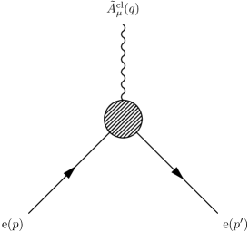
Refer to caption
Figure 1: A โ€œFeynman Diagramโ€ cartoon for lepton scattering (specifically, electron) from a static, classical background of photons, ${\tilde{A}^{\text{cl}}_{\mu}(q)}$. The shaded circle is a stand-in for the full vertex function.

The โ€œFeynman diagramโ€ for lepton-photon scattering is shown in Figureย 1. The amplitude for leptons scattering off a static (classical) background field is given by

$$i{\mathcal{M}}=-ieQ_{\mathrm{{\ell}}}{\tilde{A}^{\text{cl}}_{\mu}(q)}{\overline{\mathrm{u}}(p^{\prime})}\Gamma^{\mu}{\mathrm{u}(p)}\ ,$$ (2.1)

where the vertex operator $\Gamma^{\mu}$ can only be a function of $p^{\mu}$, ${p^{\prime}}^{\mu}$, $q^{\mu}$, $\gamma^{\mu}$, and $\gamma^{5}$. Not all combinations are independent (the Gordon identity, for example, links them). The conventional combination is written

$$\Gamma^{\mu}=F_{1}(q^{2})\gamma^{\mu}+F_{2}(q^{2})\frac{i\sigma^{\mu\nu}q_{\nu}}{2m_{\mathrm{{\ell}}}}+F_{3}(q^{2})\frac{i\sigma^{\mu\nu}q_{\nu}\gamma^{5}}{2m}\ .$$ (2.2)

The terms are chosen in this way because, in the limit $q^{2}\to 0$ (i.e. when all external particles are put on shell), the functions $F_{i}$ correspond to classical definitions of the electric charge ($F_{1}(0)$), anomalous magnetic moment ($F_{2}(0)$), and electric dipole moment ($F_{3}(0)$). Although we will not need to consider these issues, note that $F_{1}(0)$ is constrained to be 1, and thus enters as a renormalization condition. Further, $F_{3}(0)$ is strictly zero in QED, and we will not consider it further at this time. Finally, we will find that all of the integrals in the loop diagrams that give us $F_{2}(q^{2})$ are convergent, and so we will not need to involve ourselves at all in the renormalization program, although at higher loop order, this is no longer the case. To get the notation straight, let us โ€œcalculateโ€ the $F_{i}$ at tree level in QED. The amplitude for an electron scattering from a static photon background is given by

$$i{\mathcal{M}}={\overline{\mathrm{u}}(p^{\prime})}\left(-ieQ_{\mathrm{{\ell}}}\gamma^{\mu}\right){\mathrm{u}(p)}{\tilde{A}^{\text{cl}}_{\mu}(q)}\ .$$ (2.3)

Clearly, when we rearrange this as in Equationย 2.1, we find $F_{1}(q^{2})=1$ and $F_{2}(q^{2})=F_{3}(q^{2})=0$.

Note that in this work the anomalous magnetic moment of the fermion $\mathrm{{f}}$ย corresponds to

$${a_{\mathrm{{f}}}}=\frac{g_{\mathrm{{f}}}-2}{2}=F_{2}(0)\ ,$$ (2.4)

which can be compared directly to the results of the E821 collaboration.

2.2 Lagrangians and Feynman Rules

We take the following as our fermionic Lagrangian

$$\mathcal{L}={{\overline{\mathrm{{\Psi}}}_{\mathrm{{f}}}}}\left(i{\makebox[0.0pt][l]{\hskip 1.77847pt$/$}{D}}-m_{{\mathrm{{\Psi}}_{\mathrm{{f}}}}}\right){{\mathrm{{\Psi}}_{\mathrm{{f}}}}}={{\overline{\mathrm{{\Psi}}}_{\mathrm{{f}}}}}\left(i\gamma^{{\mu}}\left(\partial_{\mu}-ig\mathrm{{A}}^{\mathrm{a}}_{\mu}t^{\mathrm{a}}\right)-m_{{\mathrm{{\Psi}}_{\mathrm{{f}}}}}\right){{\mathrm{{\Psi}}_{\mathrm{{f}}}}}\ ,$$ (2.5)

which gives us the following Feynman rule for gauge-fermion coupling

$$ig\gamma^{{\mu}}t^{\mathrm{a}}\ .$$ (2.6)

The Feynman rules for scalar fields and gauge fields are more complicated to derive, and in fact, many texts with seemingly similar conventions disagree on the derived Feynman Rules; additionally, at least one text (Cheng and Li [7]) contains internally inconsistent results for some amplitudes. Although this disagreement is limited to factors of $i$ and $-1$, which does not matter when calculating most observables as they arise from squared amplitudes, these factors become very important when the observable being calculated is contained in directly in the amplitude, as is the case here.

2.2.1 Unbroken Gauge Theory

Let us consider first the Feynman rules for an unbroken gauge theory. The Lagrangian for an unbroken, non-abelian gauge theory

$$\mathcal{L}=-\frac{1}{4}{F_{\mu\nu}^{\mathrm{a}}}^{2}-\frac{1}{2\xi}\left(\partial_{\mu}A^{\mu\mathrm{a}}\right)^{2}\ ,$$ (2.7)

where the first term is

$$F_{\mu\nu}^{\mathrm{a}}=\partial_{\mu}A_{\nu}^{\mathrm{a}}-\partial_{\nu}A_{\mu}^{\mathrm{a}}+gf^{\mathrm{abc}}A_{\mu}^{\mathrm{b}}A_{\nu}^{\mathrm{c}}\ ,$$

and the second term is the Fadeev-Popov gauge fixing term, and (in this case) affects only the propagator. If we expand this term to find the trilinear and quadrilinear terms, we find (after defining $f_{\mu\nu}^{\mathrm{a}}=\partial_{\mu}A_{\nu}^{\mathrm{a}}-\partial_{\nu}A_{\mu}^{\mathrm{a}}$),

$$F_{\mu\nu}^{\mathrm{a}}F^{\mu\nu\mathrm{a}}=f_{\mu\nu}^{\mathrm{a}}f^{\mu\nu\mathrm{a}}\\ +\left(\partial_{\mu}A_{\nu}^{\mathrm{a}}-\partial_{\nu}A_{\mu}^{\mathrm{a}}\right)gf^{\mathrm{abc}}A^{\mu\mathrm{b}}A^{\nu\mathrm{c}}+gf^{\mathrm{ade}}A_{\mu}^{\mathrm{d}}A_{\nu}^{\mathrm{e}}\left(\partial^{\mu}A^{\nu\mathrm{a}}-\partial^{\nu}A^{\mu\mathrm{a}}\right)\\ +g^{2}f^{\mathrm{abc}}f^{\mathrm{ade}}A_{\mu}^{\mathrm{b}}A_{\nu}^{\mathrm{c}}A^{\mu\mathrm{d}}A^{\nu\mathrm{e}}\ .$$

The first line contributes to the propagator, the second line contributes to the trilinear gauge coupling, and the third line contributes to the quadrilinear couplings.

Let us start with the trilinear term, and derive it in detail, since various texts with supposedly identical conventions obtain results differing by factors of $i$. We need first some conventions that all the texts agree on. We label external initial state particles with incoming momenta, and external final state particles with outgoing momenta. For an external initial state gauge boson, we assign a factor

$$A_{\mu}(p)=\varepsilon_{\mu}(p)e^{-ipx}\to\partial_{\mu}A_{\nu}=-ip_{\mu}A_{\nu}\ ,$$

and for an external final state gauge boson, we assign a factor

$$A_{\nu}(p^{\prime})=\varepsilon^{*}_{\nu}(p^{\prime})e^{ip^{\prime}x}\to\partial_{\mu}A_{\nu}=ip^{\prime}_{\mu}A_{\nu}\ .$$

Then, the trilinear term in $\mathcal{L}$, with all particles considered โ€œinitial stateโ€ (i.e. with incoming momenta), is given by

$$\displaystyle\mathcal{L}\supset-\frac{1}{2}f^{\mathrm{abc}}\left(\partial_{\mu}A_{\nu}^{\mathrm{a}}\right)A^{\mu\mathrm{b}}A^{\nu\mathrm{c}}+\frac{1}{2}f^{\mathrm{abc}}\left(\partial_{\nu}A_{\mu}^{\mathrm{a}}\right)A^{\mu\mathrm{b}}A^{\nu\mathrm{c}}\ .$$
In the second term, we swap the dummy variables $\mu\leftrightarrow\nu$ and $b\leftrightarrow c$
$$\displaystyle\mathcal{L}\supset-\frac{1}{2}f^{\mathrm{abc}}\left(\partial_{\mu}A_{\nu}^{\mathrm{a}}\right)A^{\mu\mathrm{b}}A^{\nu\mathrm{c}}+\frac{1}{2}f^{\mathrm{acb}}\left(\partial_{\mu}A_{\nu}^{\mathrm{a}}\right)A^{\nu\mathrm{c}}A^{\mu\mathrm{b}}\ .$$
Now, since $f^{\mathrm{abc}}$ is completely antisymmetric, we make the substitution $f^{\mathrm{acb}}\to-f^{\mathrm{abc}}$, and obtain
$$\displaystyle-gf^{\mathrm{abc}}\left(\partial_{\mu}A_{\nu}^{\mathrm{a}}\right)A^{\mu\mathrm{b}}A^{\nu\mathrm{c}}$$
$$\displaystyle=igf^{\mathrm{abc}}k_{\mu}g^{\alpha\mu}g^{\beta\nu}A_{\nu}^{\mathrm{a}}A_{\alpha}^{\mathrm{b}}A_{\beta}^{\mathrm{c}}\ .$$

From this, we obtain a โ€œpreliminaryโ€ Feynman rule by multiplying by $i$

$$-gf^{\mathrm{abc}}k^{\alpha}g^{\beta\nu}\ .$$

Since there are $3!=6$ ways to connect the $A_{\mu}^{\mathrm{a}}$ to a trilinear vertex. At this point, to compare with the notation of [6] and [7], we relabel this to

$$-gf^{\mathrm{abc}}k^{\rho}g^{\sigma\nu}\ .$$

Summing these terms using the total antisymmetry of $f^{\mathrm{abc}}$, we obtain the Feynman rule

$$gf^{\mathrm{abc}}\left[g^{\sigma\nu}(q-k)^{\rho}+g^{\rho\nu}(k-p)^{\sigma}g^{\rho\sigma}(p-q)^{\nu}\right]\ ,$$ (2.8)

which agrees with the results of [6], but does not agree with [7], which has an additional $i$.

Similar manipulations yield the quartic coupling Feynman rule, which agrees with the results of both [6] and [7]

$$-ig^{2}\left[f^{\mathrm{abc}}f^{\mathrm{cde}}\left(g^{\mu\rho}g^{\nu\sigma}-g^{\mu\sigma}g^{\nu\rho}\right)+f^{\mathrm{ace}}f^{\mathrm{bde}}\left(g^{\mu\nu}g^{\rho\sigma}-g^{\mu\sigma}g^{\rho\nu}\right)+f^{\mathrm{ade}}f^{\mathrm{bce}}\left(g^{\mu\nu}g^{\rho\sigma}-g^{\mu\rho}g^{\nu\sigma}\right)\right]\ .$$ (2.9)

2.2.2 Complex Scalar Fields

We now approach a scalar theory coupled to an unbroken non-abelian gauge theory, and derive the scalar-vector couplings. We define the covariant derivative with the same conventions as [6] and[7]

$$D_{\mu}=\partial_{\mu}-igA_{\mu}^{\mathrm{a}}t^{\mathrm{a}}\ .$$

The minus sign here results in a plus sign in the Feynman rule for fermions, that is, $ig\gamma^{{\mu}}t^{\mathrm{a}}$. The scalar Lagrangian is

โ„’=(Dฮผโ€‹ฯ•)โ€ โ€‹(Dฮฝโ€‹ฯ•)โ€‹gฮผโ€‹ฮฝโˆ’mฯ•โ€‹ฯ•โ€ โ€‹ฯ•โˆ’ฮป4โ€‹(ฯ•โ€ โ€‹ฯ•)โ€ .โ„’superscriptsubscript๐ท๐œ‡italic-ฯ•โ€ subscript๐ท๐œˆitalic-ฯ•superscript๐‘”๐œ‡๐œˆsubscript๐‘šitalic-ฯ•superscriptitalic-ฯ•โ€ italic-ฯ•๐œ†4superscriptsuperscriptitalic-ฯ•โ€ italic-ฯ•โ€ \mathcal{L}=\left(D_{\mu}\phi\right)^{\dagger}\left(D_{\nu}\phi\right)g^{\mu\nu}-m_{\phi}\phi^{\dagger}\phi-\frac{\lambda}{4}\left(\phi^{\dagger}\phi\right)^{\dagger}\ . (2.10)

The couplings occur in the first term on the right hand side. Let us expand this term and derive the Feynman rules

$$\mathcal{L}\supset\left[\left(\partial_{\mu}-igA_{\mu}^{\mathrm{a}}t^{\mathrm{a}}\right)\phi\right]^{*}_{\ell}\left[\left(\partial_{\nu}-igA_{\nu}^{\mathrm{b}}t^{\mathrm{b}}\right)\phi\right]g^{\mu\nu}=\left(\partial_{\mu}\phi^{*}_{\ell}\right)\left(\partial_{\nu}\phi_{m}\right)g^{\mu\nu}\\ +igA_{\mu}^{\mathrm{a}}t^{\mathrm{a}}\phi^{*}_{\ell}\left(\partial_{\nu}\phi_{m}\right)g^{\mu\nu}-igA_{\nu}^{\mathrm{b}}t^{\mathrm{b}}\left(\partial_{\mu}\phi^{*}_{\ell}\right)\phi_{m}g^{\mu\nu}+g^{2}A_{\mu}^{\mathrm{a}}A_{\nu}^{\mathrm{b}}g^{\mu\nu}t^{\mathrm{a}}\phi^{*}_{\ell}t^{\mathrm{b}}\phi_{m}\ ,$$

where the first term feeds into the propagator, the second line gives rise to a scalar vector trilinear term, and the final line a quadrilinear term. First, conventions: an external scalar with incoming momentum is a $\phi$ and $\partial_{\mu}\phi=-ip_{\mu}\phi$, while a scalar with outgoing momentum is a $\phi^{*}$ and $\partial_{\mu}\phi^{*}=ip^{\prime}_{\mu}\phi^{*}$. This gives rise to a Feynman rule for trilinear terms of

$$ig\left(p^{\prime}+p\right)_{\mu}t^{\mathrm{a}}_{\ell m}\ .$$ (2.11)

The quadrilinear term is slightly more complicated, as there are two ways to connect the vectors to the vertex, so we obtain a Feynman rule

$$ig^{2}\left(t^{\mathrm{a}}t^{\mathrm{b}}\right)_{\ell m}g_{\mu\nu}+ig^{2}\left(t^{\mathrm{b}}t^{\mathrm{a}}\right)_{\ell m}g_{\mu\nu}=ig^{2}{\left\{{t^{\mathrm{a}}},{t^{\mathrm{b}}}\right\}}_{\ell m}g_{\mu\nu}\ .$$ (2.12)

In agree with [8] and with the abelian case presented in [9]. This result is not in agreement with the derivation in [7], but the results of this derivation in that text are internally inconsistent.

2.2.3 Broken Gauge Theory

In the more complicated case of broken gauge symmetry, we perform the following replacement in the Lagrangian

$$\phi\to{\left<\phi\right>}+\phi\ ,$$

which gives rise to a โ€œbilinear couplingโ€ between $A_{\mu}$ and $\phi$ that we cancel by replacing the original Fadeev-Popov gauge fixing term with

$$-\frac{1}{2\xi}\left(\partial_{\mu}A^{\mu\mathrm{a}}\right)^{2}\to-\frac{1}{2\xi}\left(\partial_{\mu}A^{\mu\mathrm{a}}+ig\xi\left(\phi^{*}t^{\mathrm{a}}{\left<\phi\right>}-{\left<\phi^{*}\right>}t^{\mathrm{a}}\phi\right)\right)^{2}\ .$$

Furthermore, this shift gives rise to an additional vector-vector-scalar coupling in the $(D\phi)^{2}$ term, and masses for the $A_{\mu}$

$$\left[igA_{\mu}^{\mathrm{a}}t^{\mathrm{a}}\left({\left<\phi^{*}\right>}+\phi^{*}\right)\right]_{\ell}\left[-igA_{\nu}^{\mathrm{b}}t^{\mathrm{b}}\left({\left<\phi^{*}\right>}+\phi^{*}\right)\right]_{m}g^{\mu\nu}=g^{2}A^{\mu\mathrm{a}}A^{\nu\mathrm{b}}g_{\mu\nu}t^{\mathrm{a}}\left({\left<\phi^{*}\right>}+\phi^{*}\right)_{\ell}t^{\mathrm{b}}\left({\left<\phi\right>}+\phi\right)_{m}\ .$$

Let us define

$$\left(t^{\mathrm{a}}{\left<\phi\right>}\right)_{\ell}=v_{\ell}^{\mathrm{a}}\ .$$

Then, the Lagrangian contains the terms

$$g^{2}A^{\mu\mathrm{a}}A^{\nu\mathrm{b}}g_{\mu\nu}\left(t_{\ell m}^{\mathrm{a}}v_{m}^{\mathrm{b}}\phi_{\ell}^{*}+t_{\ell m}^{\mathrm{b}}v_{\ell}^{\mathrm{a}}\phi_{m}+\left(t^{\mathrm{a}}t^{\mathrm{b}}\right)_{\ell m}\phi^{*}_{\ell}\phi_{m}\right)\ .$$

Since there are two ways to connect the gauge bosons in the vector-vector-scalar term, we obtain the following Feynman rule

$$ig^{2}g_{\mu\nu}t_{\ell m}^{\mathrm{a}}v_{m}^{\mathrm{b}}+ig^{2}g_{\nu\mu}t_{\ell m}^{\mathrm{b}}v_{m}^{\mathrm{a}}\ .$$ (2.13)

2.2.4 Applications to the Standard Model

How do these rules apply in the Standard Model? Consider the $\phi^{+}\mathrm{{W^{-}}}\mathrm{{\gamma}}$ coupling. Since $\mathrm{{\gamma}}_{\mu}=\mathrm{{W^{3}}}_{\mu}\sin\theta_{W}+\mathrm{{B}}_{\mu}\cos\theta_{W}$, we obtain

$$ig^{2}g_{\mu\nu}\left(0+\frac{v}{2}Q\right)\sin\theta_{W}=i(g\sin\theta_{W})\frac{gv}{2}g_{\mu\nu}Q=ieM_{\mathrm{{W}}}Qg_{\mu\nu}\ ,$$

where $Q$ is the charge of the $\phi$. This result is in agreement with [7]. Consider next the $\phi^{+}\mathrm{{W^{-}}}\mathrm{{Z^{0}}}$ coupling. Since $\mathrm{{Z^{0}}}_{\mu}=\mathrm{{W^{3}}}_{\mu}\cos\theta_{W}-\mathrm{{B}}_{\mu}\sin\theta_{W}$, and we obtain

$$ig\frac{g}{\cos\theta_{W}}g_{\mu\nu}\left(0+\frac{v}{2\cos\theta_{W}}\left(T^{3}-\sin^{2}\theta_{W}Q\right)\right)\cos\theta_{W}\\ =-ig\sin^{2}\theta_{W}g_{\mu\nu}Q\frac{gv}{2\cos\theta_{W}}=-igM_{\mathrm{{Z^{0}}}}\sin^{2}\theta_{W}Qg_{\mu\nu}\ ,$$

where, again, $Q$ is the charge of the $\phi$. This result, too, is in agreement with [7].

2.2.5 Connection between $\mathrm{{V^{\mu}}}\mathrm{{f}}\mathrm{{f^{\prime}}}$ and $\mathrm{{S_{V}}}\mathrm{{f}}\mathrm{{f^{\prime}}}$

When calculating matrix elements of interactions with internal massive vector bosons, $\mathrm{{V^{\mu}}}$, we often need to add additional diagrams with the vectors replaced by the unphysical scalars, $\mathrm{{S_{V}}}$, that exist in the theory to maintain unitarity. The question then arises, โ€œGiven the couplings between a pair of fermions and a vector, say $ig\gamma^{{\mu}}\left(a^{\mathrm{a}}+b^{\mathrm{a}}\gamma^{{5}}\right)$ for the interaction $\mathrm{{f_{i}}}\to\mathrm{{V^{\mu}}}\mathrm{{f_{e}}}$, how do we extract the corresponding coupling $ig\left(A^{\mathrm{a}}+B^{\mathrm{a}}\gamma^{{5}}\right)$ for the interaction $\mathrm{{f_{i}}}\to\mathrm{{S_{V}}}\mathrm{{f_{e}}}$?โ€ Well, since an $S$-matrix (or, correspondingly, a $T$-matrix) element must be gauge independent (independent of the chosen $R_{\xi}$ gauge parameter), if we can find a set of diagrams involving the vertices of interest, we can find the couplings $A$ and $B$ (from here on, we suppress color indices). In particular, consider the $t$-channel $\mathrm{{V^{\mu}}}$ย exchange in the process $\mathrm{{f_{i}}}\mathrm{{f^{\prime}_{i}}}\to\mathrm{{f_{e}}}\mathrm{{f^{\prime}_{e}}}$. Before writing down this matrix element, we must express the propagators of the vector and scalar. First the vector

$\displaystyle D_{\mu\nu}^{\mathrm{ab}}(k)$ $\displaystyle=\frac{-i\delta^{\mathrm{ab}}}{k^{2}-M^{2}}\left(g_{\mu\nu}-\frac{k_{\mu}k_{\nu}}{k^{2}-\xi M^{2}}(1-\xi)\right)$
$\displaystyle=\frac{-i\delta^{\mathrm{ab}}}{k^{2}-M^{2}}\left(g_{\mu\nu}-\frac{k_{\mu}k_{\nu}}{k^{2}}\right)+\frac{i\delta^{\mathrm{ab}}\xi}{k^{2}-\xi M^{2}}\left(\frac{k_{\mu}k_{\nu}}{k^{2}}\right)$
$\displaystyle=\frac{-i\delta^{\mathrm{ab}}}{k^{2}-M^{2}}\left(g_{\mu\nu}-\frac{k_{\mu}k_{\nu}}{k^{2}}\right)-\frac{i\delta^{\mathrm{ab}}}{k^{2}-\xi M^{2}}\left(\frac{k_{\mu}k_{\nu}}{M^{2}}\right)\ ,$
and second, the scalar
$\displaystyle D^{\mathrm{ab}}(k)$ $\displaystyle=\frac{i\delta^{\mathrm{ab}}}{k^{2}-\xi M^{2}}\ .$

The previously mentioned matrix element, then, is given by

$$iM=\left[{\overline{\mathrm{u}}(p^{\prime})}ig\gamma^{{\mu}}\left(a+b\gamma^{{5}}\right){\mathrm{u}(p)}\right]\left[{\overline{\mathrm{u}}(k^{\prime})}ig\gamma^{{\nu}}\left(c+d\gamma^{{5}}\right){\mathrm{u}(k)}\right]\\ \times\left[\frac{-i}{q^{2}-M^{2}}\left(g_{\mu\nu}-\frac{k_{\mu}k_{\nu}}{M^{2}}\right)-\frac{iq_{\mu}q_{\nu}}{M^{2}}\left(\frac{1}{q^{2}-\xi M^{2}}\right)\right]\\ +\left[{\overline{\mathrm{u}}(p^{\prime})}ig\left(A+B\gamma^{{5}}\right){\mathrm{u}(p)}\right]\left[{\overline{\mathrm{u}}(k^{\prime})}ig\left(C+D\gamma^{{5}}\right){\mathrm{u}(k)}\right]\frac{i}{q^{2}-\xi M^{2}}\ .$$

The $\xi$ cancellation requires the second piece of the vector propagator and the scalar propagator to cancel. Therefore, we must have

$${\overline{\mathrm{u}}(p^{\prime})}ig\left(A+B\gamma^{{5}}\right){\mathrm{u}(p)}=\pm{\overline{\mathrm{u}}(p^{\prime})}\frac{ig}{M}\leavevmode\hbox{${{\makebox[0.0pt][l]{$/$}q}}$}\left(a+b\gamma^{{5}}\right){\mathrm{u}(p)}\ .$$

Suppressing the spinor notation,

$\displaystyle A+B\gamma^{{5}}$ $\displaystyle=\pm\frac{1}{M}\left(\leavevmode\hbox{${{\makebox[0.0pt][l]{$/$}p}}$}-\leavevmode\hbox{${\smash[t]{{\makebox[0.0pt][l]{$/$}p}}^{\prime}}$}\right)\left(a+b\gamma^{{5}}\right)$
$\displaystyle=\pm\frac{1}{M}\left\{\left(a-b\gamma^{{5}}\right)\leavevmode\hbox{${{\makebox[0.0pt][l]{$/$}p}}$}-\leavevmode\hbox{${\smash[t]{{\makebox[0.0pt][l]{$/$}p}}^{\prime}}$}\left(a+b\gamma^{{5}}\right)\right\}$
$\displaystyle=\pm\frac{1}{M}\left\{\left(m_{\mathrm{i}}-m_{\mathrm{e}}\right)a-\left(m_{\mathrm{i}}+m_{\mathrm{e}}\right)b\gamma^{{5}}\right\}\ .$

The sign ambiguity is superfluous in the situation discussed here; we need only pick one convention and stick with it. Since these vertices sit at the ends of internal lines, they will come in pairs and the signs will cancel, even in matrix elements, regardless of the convention. However, if we need to include other goldstone vertices in our diagrams, we must choose a globally consistent sign. For consistency with the sign used in the vector-vector-goldstone case above, we must choose the minus sign in this note.

The Feynman rule for $\mathrm{{f_{i}}}\to\mathrm{{f_{e}}}\mathrm{{S_{V}}}$, then, will be given by $ig\left(A+B\gamma^{{5}}\right)$, where

$$\displaystyle A=\frac{m_{\mathrm{i}}-m_{\mathrm{e}}}{M}a\qquad\qquad B=-\frac{m_{\mathrm{i}}+m_{\mathrm{e}}}{M}b\ .$$ (2.14)

The Feynman rule for the conjugate process, $\mathrm{{f_{e}}}\to\mathrm{{f_{i}}}\mathrm{{S_{V}}}$, will be given by โˆ’iโ€‹gโ€‹(Aโ€ โˆ’Bโ€ โ€‹ฮณ5)๐‘–๐‘”superscript๐ดโ€ superscript๐ตโ€ superscript๐›พ5-ig\left(A^{\dagger}-B^{\dagger}\gamma^{{5}}\right) (note the minus sign with the $\gamma^{{5}}$).

2.3 Kinematic Conventions

Refer to caption
Figure 2: Definition of our kinematic variable convention.

Since we will be looking only at the one-loop, three vertex triangle diagrams, it will simplify our task if we settle on kinematic definitions once. We define the momenta as in Figureย 2. In particular, the incoming fermion carries momentum $p$ into the vertex (lower left line), the outgoing fermion carries momentum $p^{\prime}$ out of the vertex (lower right line), and the photon carries momentum $q$ into the vertex (top line). The momenta carried on the internal lines are also displayed in the figure; these will be either fermions or bosons as appropriate, but we will use the same notation for the momenta in any case.

2.4 Feynman Parameter Reduction

In calculating the amplitudes for the various diagrams of interest, we always find the product of three propagator denominators (we will make the narrow width approximation, $\Gamma=0$). These denominators will need to be combined into a result which can be integrated over the internal momentum of the loop. We will simplify the general expression obtained as much as possible.

We note the Feynman Parameter result for three distinct denominators

$$\frac{1}{ABC}=\int\limits_{0}^{1}{\mathrm{d}{x}}{\mathrm{d}{y}}{\mathrm{d}{z}}\delta(1-x-y-z)\frac{2}{\left(xA+yB+zC\right)^{3}}=\int\limits_{0}^{1}{\mathrm{d}{x}}{\mathrm{d}{y}}{\mathrm{d}{z}}\delta(1-x-y-z)\frac{2}{D^{3}}\ .$$ (2.15)

In the case of two fermions and one boson in the loop, the term $ABC$ is given by

$$ABC=\left(k^{2}-m_{\text{int}}^{2}\right)\left((k+q)^{2}-m_{\text{int}}^{2}\right)\left((p-k)^{2}-M^{2}\right)\ ,$$

which gives a $D$ term

$\displaystyle D$ $\displaystyle=x\left(k^{2}-m_{\text{int}}^{2}\right)+y\left({k^{\prime}}^{2}-m_{\text{int}}^{2}\right)+z\left((p-k)^{2}-M^{2}\right)$
$\displaystyle=(x+y+z)k^{2}-(x+y)m_{\text{int}}^{2}-zM^{2}+zp^{2}+yq^{2}+2k(yq-zp)$
substituting $p^{2}=m_{\text{ext}}^{2}$, $x+y+z=1$, and completing the square, we find
$\displaystyle=\left(k+yq-zp\right)^{2}-\left(yq-zp\right)^{2}+yq^{2}-(x+y)m_{\text{int}}^{2}-zM^{2}+zm_{\text{ext}}^{2}\ ,$

Next, expand the $-(yq-zp)^{2}+yq^{2}$ term

$\displaystyle yq^{2}-\left(yq-zp\right)^{2}$ $\displaystyle=yq^{2}-y^{2}q^{2}+2yzqp-z^{2}p^{2}$
$\displaystyle=xyq^{2}-z^{2}m_{\text{ext}}^{2}\ .$

Thus, we find

$\displaystyle D$ $\displaystyle=\left(k+yq-zp\right)^{2}+xyq^{2}-z^{2}m_{\text{ext}}^{2}+zm_{\text{ext}}^{2}-zM^{2}-(x+y)m_{\text{int}}^{2}$
$\displaystyle=\ell^{2}-\Delta+xyq^{2}\ ,$ (2.16)

where we have

$$\displaystyle\ell=k+yq-zp$$ (2.17)
$$\displaystyle\Delta=z(z-1)m_{\text{ext}}^{2}+zM^{2}+(x+y)m_{\text{int}}^{2}\ .$$ (2.18)

If we define $u=x+y$, then we can simplify this expression to read

$$\Delta=u(u-1)m_{\text{ext}}^{2}+(1-u)M^{2}+um_{\text{int}}^{2}\ .$$ (2.19)

In the case of two internal boson lines and one internal fermion line, we simply swap $m_{\text{int}}$ for $M$, and obtain

$$\Delta=u(u-1)m_{\text{ext}}^{2}+(1-u)m_{\text{int}}^{2}+uM^{2}\ .$$ (2.20)

As can be seen above, all of the integrals will be functions of $u=x+y$ alone. Therefore, it makes sense for us to change variables so that we can trivially reduce the number of integrals we have to perform. In particular, we find

$$F_{2}(0)=\int\limits_{0}^{1}{\mathrm{d}{x}}\int\limits_{0}^{1}{\mathrm{d}{y}}\int\limits_{0}^{1}{\mathrm{d}{z}}\delta(1-x-y-z)f(x+y)=\int\limits_{0}^{1}{\mathrm{d}{x}}\int\limits_{0}^{1-x}{\mathrm{d}{y}}f(x+y)\ .$$

Now, with the previous definition $u=x+y$ and defining $v=x-y$,

$$F_{2}(0)=\int\limits_{0}^{1}{\mathrm{d}{u}}\int\limits_{-u}^{u}{\mathrm{d}{v}}f(u)|J|\ .$$

The Jacobian determinant, $J$, is given by

$$J(u,v)=\left|\begin{array}[]{cc}\frac{\partial u}{\partial x}&\frac{\partial u}{\partial y}\\ \frac{\partial v}{\partial x}&\frac{\partial v}{\partial y}\end{array}\right|=-\frac{1}{2}\ .$$

And we find

$$F_{2}(0)=\int\limits_{0}^{1}{\mathrm{d}{u}}\int\limits_{-u}^{u}{\mathrm{d}{v}}f(u)|J|=\int\limits_{0}^{1}{\mathrm{d}{u}}2u\left|-\frac{1}{2}\right|f(u)=\int\limits_{0}^{1}{\mathrm{d}{u}}uf(u)\ ,$$ (2.21)

which vastly simplifies the integrals obtained in the calculations.

2.5 Relations Encountered in Numerator Reductions

In the previous section we changed integration variables from $k$ to $\ell$, defined in Equationย 2.17. We will need to use many relations to eliminate $k$ and $k^{\prime}$ in favor of $\ell$, $p$, and $p^{\prime}$, beginning with

$$\displaystyle k=\ell-yp^{\prime}+(1-x)p$$ (2.22)
$$\displaystyle k^{\prime}=\ell+(1-y)p^{\prime}-xp\ ,$$ (2.23)

when calculating the amplitudes that contain $F_{2}(0)$. In this section, we derive a number of more complicated expressions, in advance of our need for them in Sectionย 3.

We also encounter many Dirac Matrix expressions that must be reduced to functions of $\gamma^{{\mu}}$, $p^{\mu}$, and ${p^{\prime}}^{\mu}$. Below, we derive a number of relations that arise in our derivations

$$\displaystyle{\overline{\mathrm{u}}(p^{\prime})}\leavevmode\hbox{${{\makebox[0.0pt][l]{$/$}p}}$}\gamma^{{\mu}}{\mathrm{u}(p)}={\overline{\mathrm{u}}(p^{\prime})}\left(2p^{\mu}-\gamma^{{\mu}}\leavevmode\hbox{${{\makebox[0.0pt][l]{$/$}p}}$}\right){\mathrm{u}(p)}={\overline{\mathrm{u}}(p^{\prime})}\left(2p^{\mu}-m_{\text{ext}}\gamma^{{\mu}}\right){\mathrm{u}(p)}$$
$$\displaystyle{\overline{\mathrm{u}}(p^{\prime})}\gamma^{{\mu}}\leavevmode\hbox{${\smash[t]{{\makebox[0.0pt][l]{$/$}p}}^{\prime}}$}{\mathrm{u}(p)}={\overline{\mathrm{u}}(p^{\prime})}\left(2{p^{\prime}}^{\mu}-\leavevmode\hbox{${\smash[t]{{\makebox[0.0pt][l]{$/$}p}}^{\prime}}$}\gamma^{{\mu}}\right){\mathrm{u}(p)}={\overline{\mathrm{u}}(p^{\prime})}\left(2{p^{\prime}}^{\mu}-m_{\text{ext}}\gamma^{{\mu}}\right){\mathrm{u}(p)}\ ,$$

where we have used the Dirac gamma matrix relation

$$\left\{{\gamma^{{\mu}}},{\gamma^{{\nu}}}\right\}=2g^{\mu\nu}$$

We will now derive a number of similar results, suppressing the spinors.

$\displaystyle\leavevmode\hbox{${{\makebox[0.0pt][l]{$/$}p}}$}\gamma^{{\mu}}\leavevmode\hbox{${\smash[t]{{\makebox[0.0pt][l]{$/$}p}}^{\prime}}$}$ $\displaystyle=\leavevmode\hbox{${{\makebox[0.0pt][l]{$/$}p}}$}\left(2{p^{\prime}}^{\mu}-\leavevmode\hbox{${\smash[t]{{\makebox[0.0pt][l]{$/$}p}}^{\prime}}$}\gamma^{{\mu}}\right)=2m_{\text{ext}}{p^{\prime}}^{\mu}-\leavevmode\hbox{${{\makebox[0.0pt][l]{$/$}p}}$}\leavevmode\hbox{${\smash[t]{{\makebox[0.0pt][l]{$/$}p}}^{\prime}}$}\gamma^{{\mu}}$
$\displaystyle=2m_{\text{ext}}\left(p+p^{\prime}\right)^{\mu}-m_{\text{ext}}^{2}-2p\cdot p^{\prime}\gamma^{{\mu}}\ .$

But, we have

$$\displaystyle q^{2}=\left(p^{\prime}-p\right)^{2}={p^{\prime}}^{2}+p^{2}-2p\cdot p^{\prime}=2m_{\text{ext}}^{2}-2p\cdot p^{\prime}$$
$$\displaystyle\to-2p\cdot p^{\prime}=q^{2}-2m_{\text{ext}}^{2}\ ,$$

so we finally obtain

$$\leavevmode\hbox{${{\makebox[0.0pt][l]{$/$}p}}$}\gamma^{{\mu}}\leavevmode\hbox{${\smash[t]{{\makebox[0.0pt][l]{$/$}p}}^{\prime}}$}=2m_{\text{ext}}\left(p^{\prime}+p\right)^{\mu}+\left(q^{2}-3m_{\text{ext}}^{2}\right)\gamma^{{\mu}}\ ,$$

and likewise

$$\leavevmode\hbox{${\smash[t]{{\makebox[0.0pt][l]{$/$}p}}^{\prime}}$}\gamma^{{\mu}}\leavevmode\hbox{${{\makebox[0.0pt][l]{$/$}p}}$}=m_{\text{ext}}^{2}\gamma^{{\mu}}\ .$$

There are a number of additional results with two slashed $p$ momenta that we will need

$$\leavevmode\hbox{${\smash[t]{{\makebox[0.0pt][l]{$/$}p}}^{\prime}}$}\leavevmode\hbox{${\smash[t]{{\makebox[0.0pt][l]{$/$}p}}^{\prime}}$}\gamma^{{\mu}}=m_{\text{ext}}^{2}\gamma^{{\mu}}=\gamma^{{\mu}}\leavevmode\hbox{${{\makebox[0.0pt][l]{$/$}p}}$}\leavevmode\hbox{${{\makebox[0.0pt][l]{$/$}p}}$}\ .$$
$\displaystyle\leavevmode\hbox{${\smash[t]{{\makebox[0.0pt][l]{$/$}p}}^{\prime}}$}\leavevmode\hbox{${{\makebox[0.0pt][l]{$/$}p}}$}\gamma^{{\mu}}$ $\displaystyle=m_{\text{ext}}\left(2p^{\mu}-m_{\text{ext}}\gamma^{{\mu}}\right)$
$\displaystyle=2m_{\text{ext}}p^{\mu}-m_{\text{ext}}^{2}\gamma^{{\mu}}\ .$
$\displaystyle\leavevmode\hbox{${{\makebox[0.0pt][l]{$/$}p}}$}\leavevmode\hbox{${\smash[t]{{\makebox[0.0pt][l]{$/$}p}}^{\prime}}$}\gamma^{{\mu}}$ $\displaystyle=\left(2p\cdot p^{\prime}-\leavevmode\hbox{${\smash[t]{{\makebox[0.0pt][l]{$/$}p}}^{\prime}}$}\leavevmode\hbox{${{\makebox[0.0pt][l]{$/$}p}}$}\right)\gamma^{{\mu}}$
$\displaystyle=\left(2m_{\text{ext}}^{2}-q^{2}\right)\gamma^{{\mu}}-m_{\text{ext}}\left(2p^{\mu}-m_{\text{ext}}\gamma^{{\mu}}\right)$
$\displaystyle=\left(3m_{\text{ext}}^{2}-q^{2}\right)\gamma^{{\mu}}-2m_{\text{ext}}p^{\mu}\ .$
$\displaystyle\leavevmode\hbox{${{\makebox[0.0pt][l]{$/$}p}}$}\leavevmode\hbox{${{\makebox[0.0pt][l]{$/$}p}}$}\gamma^{{\mu}}$ $\displaystyle=\leavevmode\hbox{${{\makebox[0.0pt][l]{$/$}p}}$}\left(2p^{\mu}-m_{\text{ext}}\gamma^{{\mu}}\right)$
$\displaystyle=2m_{\text{ext}}p^{\mu}-m_{\text{ext}}\left(2p^{\mu}-m_{\text{ext}}\gamma^{{\mu}}\right)$
$\displaystyle=m_{\text{ext}}^{2}\gamma^{{\mu}}$
$\displaystyle=\gamma^{{\mu}}\leavevmode\hbox{${\smash[t]{{\makebox[0.0pt][l]{$/$}p}}^{\prime}}$}\leavevmode\hbox{${\smash[t]{{\makebox[0.0pt][l]{$/$}p}}^{\prime}}$}\ .$
$\displaystyle\gamma^{{\mu}}\leavevmode\hbox{${\smash[t]{{\makebox[0.0pt][l]{$/$}p}}^{\prime}}$}\leavevmode\hbox{${{\makebox[0.0pt][l]{$/$}p}}$}$ $\displaystyle=m_{\text{ext}}\left(2{p^{\prime}}^{\mu}-m_{\text{ext}}\gamma^{{\mu}}\right)$
$\displaystyle=2m_{\text{ext}}{p^{\prime}}^{\mu}-m_{\text{ext}}^{2}\gamma^{{\mu}}\ .$
$\displaystyle\gamma^{{\mu}}\leavevmode\hbox{${{\makebox[0.0pt][l]{$/$}p}}$}\leavevmode\hbox{${\smash[t]{{\makebox[0.0pt][l]{$/$}p}}^{\prime}}$}$ $\displaystyle=\gamma^{{\mu}}\left(2p^{\prime}\cdot p-\leavevmode\hbox{${\smash[t]{{\makebox[0.0pt][l]{$/$}p}}^{\prime}}$}\leavevmode\hbox{${{\makebox[0.0pt][l]{$/$}p}}$}\right)$
$\displaystyle=\left(2m_{\text{ext}}^{2}-q^{2}\right)\gamma^{{\mu}}-m_{\text{ext}}\left(2{p^{\prime}}^{\mu}-m_{\text{ext}}\gamma^{{\mu}}\right)$
$\displaystyle=\left(3m_{\text{ext}}^{2}-q^{2}\right)\gamma^{{\mu}}-2m_{\text{ext}}{p^{\prime}}^{\mu}\ .$

The next relations involve single terms in ย /โ€‹kย /๐‘˜{{\makebox[0.0pt][l]{\hskip 0.26042pt$/$}k}} and ย /โ€‹kโ€ฒย /superscript๐‘˜โ€ฒ{\smash[t]{{\makebox[0.0pt][l]{\hskip 0.26042pt$/$}k}}^{\prime}}.

ย /โ€‹kโ€‹ฮณฮผย /๐‘˜superscript๐›พ๐œ‡\displaystyle\leavevmode\hbox{${{\makebox[0.0pt][l]{\hskip 0.26042pt$/$}k}}$}\gamma^{{\mu}} =(/โ„“โˆ’yโ€‹/pโ€ฒ+(1โˆ’x)โ€‹/p)โ€‹ฮณฮผabsentabsentโ„“๐‘ฆabsentsuperscript๐‘โ€ฒ1๐‘ฅabsent๐‘superscript๐›พ๐œ‡\displaystyle=\left(\leavevmode\hbox{${{\makebox[0.0pt][l]{$/$}\ell}}$}-y\leavevmode\hbox{${\smash[t]{{\makebox[0.0pt][l]{$/$}p}}^{\prime}}$}+(1-x)\leavevmode\hbox{${{\makebox[0.0pt][l]{$/$}p}}$}\right)\gamma^{{\mu}}
$\displaystyle=\leavevmode\hbox{${{\makebox[0.0pt][l]{$/$}\ell}}$}\gamma^{{\mu}}-ym_{\text{ext}}\gamma^{{\mu}}+(1-x)\left(2p^{\mu}-m_{\text{ext}}\gamma^{{\mu}}\right)$
$\displaystyle=\leavevmode\hbox{${{\makebox[0.0pt][l]{$/$}\ell}}$}\gamma^{{\mu}}+2(1-x)p^{\mu}-\left(1-(x-y)\right)m_{\text{ext}}\gamma^{{\mu}}\ .$
$\displaystyle\gamma^{{\mu}}\leavevmode\hbox{${{\makebox[0.0pt][l]{\hskip 0.26042pt$/$}k}}$}$ $\displaystyle=\gamma^{{\mu}}\left(\leavevmode\hbox{${{\makebox[0.0pt][l]{$/$}\ell}}$}-y\leavevmode\hbox{${\smash[t]{{\makebox[0.0pt][l]{$/$}p}}^{\prime}}$}+(1-x)\leavevmode\hbox{${{\makebox[0.0pt][l]{$/$}p}}$}\right)$
$\displaystyle=\gamma^{{\mu}}\leavevmode\hbox{${{\makebox[0.0pt][l]{$/$}\ell}}$}-y\left(2{p^{\prime}}^{\mu}-m_{\text{ext}}\gamma^{{\mu}}\right)+(1-x)m_{\text{ext}}\gamma^{{\mu}}$
$\displaystyle=\gamma^{{\mu}}\leavevmode\hbox{${{\makebox[0.0pt][l]{$/$}\ell}}$}-2y{p^{\prime}}^{\mu}+\left(1-(x-y)\right)m_{\text{ext}}\gamma^{{\mu}}\ .$
ย /โ€‹kโ€ฒโ€‹ฮณฮผย /superscript๐‘˜โ€ฒsuperscript๐›พ๐œ‡\displaystyle\leavevmode\hbox{${\smash[t]{{\makebox[0.0pt][l]{\hskip 0.26042pt$/$}k}}^{\prime}}$}\gamma^{{\mu}} =(/โ„“+(1โˆ’y)โ€‹/pโ€ฒโˆ’xโ€‹/p)โ€‹ฮณฮผabsentabsentโ„“1๐‘ฆabsentsuperscript๐‘โ€ฒ๐‘ฅabsent๐‘superscript๐›พ๐œ‡\displaystyle=\left(\leavevmode\hbox{${{\makebox[0.0pt][l]{$/$}\ell}}$}+(1-y)\leavevmode\hbox{${\smash[t]{{\makebox[0.0pt][l]{$/$}p}}^{\prime}}$}-x\leavevmode\hbox{${{\makebox[0.0pt][l]{$/$}p}}$}\right)\gamma^{{\mu}}
$\displaystyle=\leavevmode\hbox{${{\makebox[0.0pt][l]{$/$}\ell}}$}\gamma^{{\mu}}+(1-y)m_{\text{ext}}\gamma^{{\mu}}-x\left(2p^{\mu}-m_{\text{ext}}\gamma^{{\mu}}\right)$
$\displaystyle=\leavevmode\hbox{${{\makebox[0.0pt][l]{$/$}\ell}}$}\gamma^{{\mu}}-2xp^{\mu}+\left(1+(x-y)\right)m_{\text{ext}}\gamma^{{\mu}}\ .$
$\displaystyle\gamma^{{\mu}}\leavevmode\hbox{${\smash[t]{{\makebox[0.0pt][l]{\hskip 0.26042pt$/$}k}}^{\prime}}$}$ $\displaystyle=\gamma^{{\mu}}\left(\leavevmode\hbox{${{\makebox[0.0pt][l]{$/$}\ell}}$}+(1-y)\leavevmode\hbox{${\smash[t]{{\makebox[0.0pt][l]{$/$}p}}^{\prime}}$}-x\leavevmode\hbox{${{\makebox[0.0pt][l]{$/$}p}}$}\right)$
$\displaystyle=\gamma^{{\mu}}\leavevmode\hbox{${{\makebox[0.0pt][l]{$/$}\ell}}$}+(1-y)\left(2{p^{\prime}}^{\mu}-m_{\text{ext}}\gamma^{{\mu}}\right)-xm_{\text{ext}}\gamma^{{\mu}}$
$\displaystyle=\gamma^{{\mu}}\leavevmode\hbox{${{\makebox[0.0pt][l]{$/$}\ell}}$}+2(1-y){p^{\prime}}^{\mu}-\left(1+(x-y)\right)m_{\text{ext}}\gamma^{{\mu}}\ .$

These results for slashed $k$ and $k^{\prime}$ terms will appear in the amplitudes we calculate the combinations below. Additionally, terms in $F_{2}(0)$ which depend on only one factor of $\ell$ (or ${{\makebox[0.0pt][l]{$/$}\ell}}$) will yield zero on integration over ${\mathrm{d}^{4}{\ell}}$. Thus, from here on we will drop all terms which carry a single $\ell$. When we drop terms, we will note that we have done so by using the notation $\Rightarrow$. Referring back to the definition of the fermion-photon vertex function, note that we are looking for the coefficients of terms $\sigma^{\mu\nu}q_{\nu}$, Equationย 2.2. We will obtain these by finding terms in $p^{\prime}+p$, and using the Gordon Identity [6]

$${\overline{\mathrm{u}}(p^{\prime})}\gamma^{{\mu}}{\mathrm{u}(p)}=\frac{1}{2m_{\text{ext}}}{\overline{\mathrm{u}}(p^{\prime})}\left(\left(p^{\prime}+p\right)^{\mu}+i\sigma^{\mu\nu}q_{\nu}\right){\mathrm{u}(p)}\ ,$$ (2.24)

to exchange those for the terms we want. The extra terms in $\gamma^{{\mu}}$ that arise when we perform this substitution contribute to $F_{1}(0)$, and can also be dropped in our calculations.

ย /โ€‹kโ€‹ฮณฮผ+ฮณฮผโ€‹ย /โ€‹kโ€ฒโ‡’2โ€‹(1โˆ’x)โ€‹pฮผ+2โ€‹(1โˆ’y)โ€‹pโ€ฒฮผโ‡’(2โˆ’(x+y))โ€‹(pโ€ฒ+p)ฮผ=(2โˆ’u)โ€‹(pโ€ฒ+p)ฮผโ‡’ย /๐‘˜superscript๐›พ๐œ‡superscript๐›พ๐œ‡ย /superscript๐‘˜โ€ฒ21๐‘ฅsuperscript๐‘๐œ‡21๐‘ฆsuperscriptsuperscript๐‘โ€ฒ๐œ‡โ‡’2๐‘ฅ๐‘ฆsuperscriptsuperscript๐‘โ€ฒ๐‘๐œ‡2๐‘ขsuperscriptsuperscript๐‘โ€ฒ๐‘๐œ‡\displaystyle\leavevmode\hbox{${{\makebox[0.0pt][l]{\hskip 0.26042pt$/$}k}}$}\gamma^{{\mu}}+\gamma^{{\mu}}\leavevmode\hbox{${\smash[t]{{\makebox[0.0pt][l]{\hskip 0.26042pt$/$}k}}^{\prime}}$}\Rightarrow 2(1-x)p^{\mu}+2(1-y){p^{\prime}}^{\mu}\Rightarrow\left(2-(x+y)\right)\left(p^{\prime}+p\right)^{\mu}=(2-u)\left(p^{\prime}+p\right)^{\mu}
$$\displaystyle\gamma^{{\mu}}\leavevmode\hbox{${{\makebox[0.0pt][l]{\hskip 0.26042pt$/$}k}}$}+\leavevmode\hbox{${\smash[t]{{\makebox[0.0pt][l]{\hskip 0.26042pt$/$}k}}^{\prime}}$}\gamma^{{\mu}}\Rightarrow-2y{p^{\prime}}^{\mu}-2xp^{\mu}\Rightarrow-(x+y)\left(p^{\prime}+p\right)^{\mu}=-u\left(p^{\prime}+p\right)^{\mu}\ .$$
ย /โ€‹kโ€‹ฮณฮผโ€‹ย /โ€‹kโ€ฒย /๐‘˜superscript๐›พ๐œ‡ย /superscript๐‘˜โ€ฒ\displaystyle\leavevmode\hbox{${{\makebox[0.0pt][l]{\hskip 0.26042pt$/$}k}}$}\gamma^{{\mu}}\leavevmode\hbox{${\smash[t]{{\makebox[0.0pt][l]{\hskip 0.26042pt$/$}k}}^{\prime}}$} =[/โ„“โˆ’yโ€‹/pโ€ฒ+(1โˆ’x)โ€‹/p]โ€‹ฮณฮผโ€‹[/โ„“+(1โˆ’y)โ€‹/pโ€ฒโˆ’xโ€‹/p]absentdelimited-[]absentโ„“๐‘ฆabsentsuperscript๐‘โ€ฒ1๐‘ฅabsent๐‘superscript๐›พ๐œ‡delimited-[]absentโ„“1๐‘ฆabsentsuperscript๐‘โ€ฒ๐‘ฅabsent๐‘\displaystyle=\left[\leavevmode\hbox{${{\makebox[0.0pt][l]{$/$}\ell}}$}-y\leavevmode\hbox{${\smash[t]{{\makebox[0.0pt][l]{$/$}p}}^{\prime}}$}+(1-x)\leavevmode\hbox{${{\makebox[0.0pt][l]{$/$}p}}$}\right]\gamma^{{\mu}}\left[\leavevmode\hbox{${{\makebox[0.0pt][l]{$/$}\ell}}$}+(1-y)\leavevmode\hbox{${\smash[t]{{\makebox[0.0pt][l]{$/$}p}}^{\prime}}$}-x\leavevmode\hbox{${{\makebox[0.0pt][l]{$/$}p}}$}\right]
$\displaystyle=\left[\leavevmode\hbox{${{\makebox[0.0pt][l]{$/$}\ell}}$}-ym_{\text{ext}}+(1-x)\leavevmode\hbox{${{\makebox[0.0pt][l]{$/$}p}}$}\right]\gamma^{{\mu}}\left[\leavevmode\hbox{${{\makebox[0.0pt][l]{$/$}\ell}}$}+(1-y)\leavevmode\hbox{${\smash[t]{{\makebox[0.0pt][l]{$/$}p}}^{\prime}}$}-xm_{\text{ext}}\right]$
$\displaystyle\Rightarrow-y(1-y)m_{\text{ext}}\gamma^{{\mu}}\leavevmode\hbox{${\smash[t]{{\makebox[0.0pt][l]{$/$}p}}^{\prime}}$}-x(1-x)m_{\text{ext}}\leavevmode\hbox{${{\makebox[0.0pt][l]{$/$}p}}$}\gamma^{{\mu}}+(1-x)(1-y)\leavevmode\hbox{${{\makebox[0.0pt][l]{$/$}p}}$}\gamma^{{\mu}}\leavevmode\hbox{${\smash[t]{{\makebox[0.0pt][l]{$/$}p}}^{\prime}}$}$
$\displaystyle\Rightarrow-2y(1-y)m_{\text{ext}}{p^{\prime}}^{\mu}-2x(1-x)m_{\text{ext}}p^{\mu}+2(1-x)(1-y)m_{\text{ext}}\left(p^{\prime}+p\right)^{\mu}$
$\displaystyle=-m_{\text{ext}}\left(y(1-y)+x(1-x)-2(1-x)(1-y)\right)\left(p^{\prime}+p\right)^{\mu}+m_{\text{ext}}\left(-x(1-x)+y(1-y)\right)\left(p^{\prime}-p\right)^{\mu}$
but since the final term is odd in $x\leftrightarrow y$ while the denominator and integrals are even, the $p^{\prime}-p$ term vanishes, so
$\displaystyle=-m_{\text{ext}}\left(p^{\prime}+p\right)^{\mu}\left(y+x-y^{2}-x^{2}-2xy-2+2(x+y)\right)$
$\displaystyle=-m_{\text{ext}}\left(p^{\prime}+p\right)^{\mu}\left(2(x+y)-(x+y)^{2}-2\right)$
Performing the $u=x+y$ substitution
$\displaystyle=m_{\text{ext}}\left(p^{\prime}+p\right)^{\mu}\left(u^{2}-3u+2\right)$
$\displaystyle=m_{\text{ext}}\left(p^{\prime}+p\right)^{\mu}(u-1)(u-2)\ .$

And finally,

ย /โ€‹kโ€ฒโ€‹ฮณฮผโ€‹ย /โ€‹kย /superscript๐‘˜โ€ฒsuperscript๐›พ๐œ‡ย /๐‘˜\displaystyle\leavevmode\hbox{${\smash[t]{{\makebox[0.0pt][l]{\hskip 0.26042pt$/$}k}}^{\prime}}$}\gamma^{{\mu}}\leavevmode\hbox{${{\makebox[0.0pt][l]{\hskip 0.26042pt$/$}k}}$} =[/โ„“+(1โˆ’y)โ€‹/pโ€ฒโˆ’xโ€‹/p]โ€‹ฮณฮผโ€‹[/โ„“โˆ’yโ€‹/pโ€ฒ+(1โˆ’x)โ€‹/p]absentdelimited-[]absentโ„“1๐‘ฆabsentsuperscript๐‘โ€ฒ๐‘ฅabsent๐‘superscript๐›พ๐œ‡delimited-[]absentโ„“๐‘ฆabsentsuperscript๐‘โ€ฒ1๐‘ฅabsent๐‘\displaystyle=\left[\leavevmode\hbox{${{\makebox[0.0pt][l]{$/$}\ell}}$}+(1-y)\leavevmode\hbox{${\smash[t]{{\makebox[0.0pt][l]{$/$}p}}^{\prime}}$}-x\leavevmode\hbox{${{\makebox[0.0pt][l]{$/$}p}}$}\right]\gamma^{{\mu}}\left[\leavevmode\hbox{${{\makebox[0.0pt][l]{$/$}\ell}}$}-y\leavevmode\hbox{${\smash[t]{{\makebox[0.0pt][l]{$/$}p}}^{\prime}}$}+(1-x)\leavevmode\hbox{${{\makebox[0.0pt][l]{$/$}p}}$}\right]
$\displaystyle\Rightarrow\left[(1-y)m_{\text{ext}}-x\leavevmode\hbox{${{\makebox[0.0pt][l]{$/$}p}}$}\right]\gamma^{{\mu}}\left[-y\leavevmode\hbox{${\smash[t]{{\makebox[0.0pt][l]{$/$}p}}^{\prime}}$}+(1-x)m_{\text{ext}}\right]$
$\displaystyle\Rightarrow-y(1-y)m_{\text{ext}}\gamma^{{\mu}}\leavevmode\hbox{${\smash[t]{{\makebox[0.0pt][l]{$/$}p}}^{\prime}}$}-x(1-x)m_{\text{ext}}\leavevmode\hbox{${{\makebox[0.0pt][l]{$/$}p}}$}\gamma^{{\mu}}+xy\leavevmode\hbox{${{\makebox[0.0pt][l]{$/$}p}}$}\gamma^{{\mu}}\leavevmode\hbox{${\smash[t]{{\makebox[0.0pt][l]{$/$}p}}^{\prime}}$}$
$\displaystyle\Rightarrow-2y(1-y)m_{\text{ext}}{p^{\prime}}^{\mu}-2x(1-x)m_{\text{ext}}p^{\mu}+2xym_{\text{ext}}\left(p^{\prime}+p\right)^{\mu}$
$\displaystyle=m_{\text{ext}}\left(-y(1-y)-x(1-x)+2xy\right)\left(p^{\prime}+p\right)^{\mu}$
$\displaystyle=m_{\text{ext}}\left(p^{\prime}+p\right)\left((x+y)^{2}-(x+y)\right)$
Performing the $u=x+y$ substitution, we find
$\displaystyle=m_{\text{ext}}\left(p^{\prime}+p\right)^{\mu}\left(u^{2}-u\right)$
$\displaystyle=m_{\text{ext}}\left(p^{\prime}+p\right)^{\mu}u(u-1)\ .$

To summarize, then, the contributions to the numerator of $F_{2}(0)$ arising from each of these terms are

$$\displaystyle\gamma^{{\mu}}\leavevmode\hbox{${{\makebox[0.0pt][l]{$/$}p}}$}\Mapsto 0$$ (2.25)
$$\displaystyle\gamma^{{\mu}}\leavevmode\hbox{${\smash[t]{{\makebox[0.0pt][l]{$/$}p}}^{\prime}}$}\Mapsto 2{p^{\prime}}^{\mu}$$ (2.26)
$$\displaystyle\leavevmode\hbox{${{\makebox[0.0pt][l]{$/$}p}}$}\gamma^{{\mu}}\Mapsto 2p^{\mu}$$ (2.27)
$$\displaystyle\leavevmode\hbox{${\smash[t]{{\makebox[0.0pt][l]{$/$}p}}^{\prime}}$}\gamma^{{\mu}}\Mapsto 0$$ (2.28)
$$\displaystyle\leavevmode\hbox{${\smash[t]{{\makebox[0.0pt][l]{$/$}p}}^{\prime}}$}\leavevmode\hbox{${\smash[t]{{\makebox[0.0pt][l]{$/$}p}}^{\prime}}$}\gamma^{{\mu}}\Mapsto 0$$ (2.29)
$$\displaystyle\leavevmode\hbox{${\smash[t]{{\makebox[0.0pt][l]{$/$}p}}^{\prime}}$}\leavevmode\hbox{${{\makebox[0.0pt][l]{$/$}p}}$}\gamma^{{\mu}}\Mapsto 2m_{\text{ext}}p^{\mu}$$ (2.30)
$$\displaystyle\leavevmode\hbox{${{\makebox[0.0pt][l]{$/$}p}}$}\leavevmode\hbox{${\smash[t]{{\makebox[0.0pt][l]{$/$}p}}^{\prime}}$}\gamma^{{\mu}}\Mapsto-2m_{\text{ext}}p^{\mu}$$ (2.31)
$$\displaystyle\leavevmode\hbox{${{\makebox[0.0pt][l]{$/$}p}}$}\leavevmode\hbox{${{\makebox[0.0pt][l]{$/$}p}}$}\gamma^{{\mu}}\Mapsto 0$$ (2.32)
$$\displaystyle\gamma^{{\mu}}\leavevmode\hbox{${{\makebox[0.0pt][l]{$/$}p}}$}\leavevmode\hbox{${{\makebox[0.0pt][l]{$/$}p}}$}\Mapsto 0$$ (2.33)
$$\displaystyle\gamma^{{\mu}}\leavevmode\hbox{${\smash[t]{{\makebox[0.0pt][l]{$/$}p}}^{\prime}}$}\leavevmode\hbox{${{\makebox[0.0pt][l]{$/$}p}}$}\Mapsto 2m_{\text{ext}}{p^{\prime}}^{\mu}$$ (2.34)
$$\displaystyle\gamma^{{\mu}}\leavevmode\hbox{${{\makebox[0.0pt][l]{$/$}p}}$}\leavevmode\hbox{${\smash[t]{{\makebox[0.0pt][l]{$/$}p}}^{\prime}}$}\Mapsto-2m_{\text{ext}}{p^{\prime}}^{\mu}$$ (2.35)
$$\displaystyle\gamma^{{\mu}}\leavevmode\hbox{${\smash[t]{{\makebox[0.0pt][l]{$/$}p}}^{\prime}}$}\leavevmode\hbox{${\smash[t]{{\makebox[0.0pt][l]{$/$}p}}^{\prime}}$}\Mapsto 0$$ (2.36)
ย /โ€‹kโ€‹ฮณฮผ+ฮณฮผโ€‹ย /โ€‹kโ€ฒโค‡โˆ’iโ€‹ฯƒฮผโ€‹ฮฝโ€‹qฮฝโ€‹(2โˆ’u)=iโ€‹ฯƒฮผโ€‹ฮฝโ€‹qฮฝโ€‹[uโˆ’2]โค‡ย /๐‘˜superscript๐›พ๐œ‡superscript๐›พ๐œ‡ย /superscript๐‘˜โ€ฒ๐‘–superscript๐œŽ๐œ‡๐œˆsubscript๐‘ž๐œˆ2๐‘ข๐‘–superscript๐œŽ๐œ‡๐œˆsubscript๐‘ž๐œˆdelimited-[]๐‘ข2\displaystyle\leavevmode\hbox{${{\makebox[0.0pt][l]{\hskip 0.26042pt$/$}k}}$}\gamma^{{\mu}}+\gamma^{{\mu}}\leavevmode\hbox{${\smash[t]{{\makebox[0.0pt][l]{\hskip 0.26042pt$/$}k}}^{\prime}}$}\Mapsto-i\sigma^{\mu\nu}q_{\nu}(2-u)=i\sigma^{\mu\nu}q_{\nu}\left[u-2\right] (2.37)
$$\displaystyle\gamma^{{\mu}}\leavevmode\hbox{${{\makebox[0.0pt][l]{\hskip 0.26042pt$/$}k}}$}+\leavevmode\hbox{${\smash[t]{{\makebox[0.0pt][l]{\hskip 0.26042pt$/$}k}}^{\prime}}$}\gamma^{{\mu}}\Mapsto i\sigma^{\mu\nu}q_{\nu}\left[u\right]$$ (2.38)
ย /โ€‹kโ€‹ฮณฮผโ€‹ย /โ€‹kโ€ฒโค‡โˆ’iโ€‹ฯƒฮผโ€‹ฮฝโ€‹qฮฝโ€‹mextโ€‹(uโˆ’1)โ€‹(uโˆ’2)=iโ€‹ฯƒฮผโ€‹ฮฝโ€‹qฮฝโ€‹[โˆ’mextโ€‹(uโˆ’1)โ€‹(uโˆ’2)]โค‡ย /๐‘˜superscript๐›พ๐œ‡ย /superscript๐‘˜โ€ฒ๐‘–superscript๐œŽ๐œ‡๐œˆsubscript๐‘ž๐œˆsubscript๐‘šext๐‘ข1๐‘ข2๐‘–superscript๐œŽ๐œ‡๐œˆsubscript๐‘ž๐œˆdelimited-[]subscript๐‘šext๐‘ข1๐‘ข2\displaystyle\leavevmode\hbox{${{\makebox[0.0pt][l]{\hskip 0.26042pt$/$}k}}$}\gamma^{{\mu}}\leavevmode\hbox{${\smash[t]{{\makebox[0.0pt][l]{\hskip 0.26042pt$/$}k}}^{\prime}}$}\Mapsto-i\sigma^{\mu\nu}q_{\nu}m_{\text{ext}}(u-1)(u-2)=i\sigma^{\mu\nu}q_{\nu}\left[-m_{\text{ext}}(u-1)(u-2)\right] (2.39)
ย /โ€‹kโ€ฒโ€‹ฮณฮผโ€‹ย /โ€‹kโค‡โˆ’iโ€‹ฯƒฮผโ€‹ฮฝโ€‹qฮฝโ€‹mextโ€‹uโ€‹(uโˆ’1)=iโ€‹ฯƒฮผโ€‹ฮฝโ€‹qฮฝโ€‹[mextโ€‹uโ€‹(1โˆ’u)].โค‡ย /superscript๐‘˜โ€ฒsuperscript๐›พ๐œ‡ย /๐‘˜๐‘–superscript๐œŽ๐œ‡๐œˆsubscript๐‘ž๐œˆsubscript๐‘šext๐‘ข๐‘ข1๐‘–superscript๐œŽ๐œ‡๐œˆsubscript๐‘ž๐œˆdelimited-[]subscript๐‘šext๐‘ข1๐‘ข\displaystyle\leavevmode\hbox{${\smash[t]{{\makebox[0.0pt][l]{\hskip 0.26042pt$/$}k}}^{\prime}}$}\gamma^{{\mu}}\leavevmode\hbox{${{\makebox[0.0pt][l]{\hskip 0.26042pt$/$}k}}$}\Mapsto-i\sigma^{\mu\nu}q_{\nu}m_{\text{ext}}u(u-1)=i\sigma^{\mu\nu}q_{\nu}\left[m_{\text{ext}}u(1-u)\right]\ . (2.40)

3 A Systematic Approach: Using the Tools

Having derived needed tools, or โ€œbuilding blocksโ€ for our one loop calculation, we now turn to the calculation of the four classes of diagrams to ${a_{\mathrm{{\mu}}}}$: neutral and charged scalars and neutral and charged vectors.

3.1 Neutral/Charged Scalar Contributions

3.1.1 Summary

Refer to caption
Figure 3: This Feynman diagram gives a one-loop contribution to ${a_{\mathrm{{f}}}}$ย from neutral/charged scalars.

Electrically neutral and charged scalar contributes the following term to the anomalous magnetic moment of a charged fermion:

aext=mextโ€‹g28โ€‹ฯ€2โ€‹QintQextโ€‹โˆซ01duโ€‹u2โ€‹mintโ€‹(vโ€‹vโ€ โˆ’aโ€‹aโ€ )โˆ’mextโ€‹(vโ€‹vโ€ +aโ€‹aโ€ )โ€‹(uโˆ’1)(1โˆ’u)โ€‹M2+uโ€‹mint2+uโ€‹(uโˆ’1)โ€‹mext2.subscript๐‘Žextsubscript๐‘šextsuperscript๐‘”28superscript๐œ‹2subscript๐‘„intsubscript๐‘„extsuperscriptsubscript01differential-d๐‘ขsuperscript๐‘ข2subscript๐‘šint๐‘ฃsuperscript๐‘ฃโ€ ๐‘Žsuperscript๐‘Žโ€ subscript๐‘šext๐‘ฃsuperscript๐‘ฃโ€ ๐‘Žsuperscript๐‘Žโ€ ๐‘ข11๐‘ขsuperscript๐‘€2๐‘ขsuperscriptsubscript๐‘šint2๐‘ข๐‘ข1superscriptsubscript๐‘šext2{a_{\text{ext}}}=\frac{m_{\text{ext}}g^{2}}{8\pi^{2}}\frac{Q_{\text{int}}}{Q_{\text{ext}}}\int\limits_{0}^{1}{\mathrm{d}{u}}u^{2}\frac{m_{\text{int}}\left(vv^{\dagger}-aa^{\dagger}\right)-m_{\text{ext}}\left(vv^{\dagger}+aa^{\dagger}\right)(u-1)}{(1-u)M^{2}+um_{\text{int}}^{2}+u(u-1)m_{\text{ext}}^{2}}\ . (3.1)

The Feynman diagram contributing to this term is found in Figureย 3.

3.1.2 The Calculation

We calculate the contribution of a scalar that couples to a pair of fermions $\mathrm{{f_{\text{int}}}}\to\mathrm{{f_{\text{ext}}}}\mathrm{{S}}$ with Feyman Rule $ig(v+a\gamma^{{5}})$, that is, with arbitrary vector and axial couplings. The matrix element is given by

$\displaystyle i{\mathcal{M}}$ $\displaystyle=ieQ_{e}{\overline{\mathrm{u}}(p^{\prime})}\Gamma^{\mu}{\mathrm{u}(p)}$
=โˆซd4โ€‹k(2โ€‹ฯ€)4โ€‹uยฏโ€‹(pโ€ฒ)โ€‹iโ€‹gโ€‹(v+aโ€‹ฮณ5)โ€‹iโ€‹(ย /โ€‹kโ€ฒ+mint)kโ€ฒ2โˆ’mint2โ€‹iโ€‹eโ€‹Qintโ€‹ฮณฮผโ€‹iโ€‹(ย /โ€‹k+mint)k2โˆ’mint2โ€‹iโ€‹gโ€‹(vโ€ โˆ’aโ€ โ€‹ฮณ5)โ€‹uโ€‹(p)โ€‹i(pโˆ’k)2โˆ’M2absentsuperscriptd4๐‘˜superscript2๐œ‹4ยฏusuperscript๐‘โ€ฒ๐‘–๐‘”๐‘ฃ๐‘Žsuperscript๐›พ5๐‘–ย /superscript๐‘˜โ€ฒsubscript๐‘šintsuperscriptsuperscript๐‘˜โ€ฒ2superscriptsubscript๐‘šint2๐‘–๐‘’subscript๐‘„intsuperscript๐›พ๐œ‡๐‘–ย /๐‘˜subscript๐‘šintsuperscript๐‘˜2superscriptsubscript๐‘šint2๐‘–๐‘”superscript๐‘ฃโ€ superscript๐‘Žโ€ superscript๐›พ5u๐‘๐‘–superscript๐‘๐‘˜2superscript๐‘€2\displaystyle=\int\frac{{\mathrm{d}^{4}{k}}}{(2\pi)^{4}}{\overline{\mathrm{u}}(p^{\prime})}ig\left(v+a\gamma^{{5}}\right)\frac{i(\leavevmode\hbox{${\smash[t]{{\makebox[0.0pt][l]{\hskip 0.26042pt$/$}k}}^{\prime}}$}+m_{\text{int}})}{{k^{\prime}}^{2}-m_{\text{int}}^{2}}ieQ_{\text{int}}\gamma^{{\mu}}\frac{i(\leavevmode\hbox{${{\makebox[0.0pt][l]{\hskip 0.26042pt$/$}k}}$}+m_{\text{int}})}{k^{2}-m_{\text{int}}^{2}}ig\left(v^{\dagger}-a^{\dagger}\gamma^{{5}}\right){\mathrm{u}(p)}\frac{i}{(p-k)^{2}-M^{2}}
=iโ€‹eโ€‹Qextโ€‹QintQextโ€‹โˆซd4โ€‹k(2โ€‹ฯ€)4โ€‹g2โ€‹i5โ€‹uยฏโ€‹(pโ€ฒ)โ€‹(v+aโ€‹ฮณ5)โ€‹(ย /โ€‹kโ€ฒ+mint)โ€‹ฮณฮผโ€‹(ย /โ€‹k+mint)โ€‹(vโ€ โˆ’aโ€ โ€‹ฮณ5)(k2โˆ’mint2)โ€‹(kโ€ฒ2โˆ’mint2)โ€‹((pโˆ’k)2โˆ’M2)โ€‹uโ€‹(p).absent๐‘–๐‘’subscript๐‘„extsubscript๐‘„intsubscript๐‘„extsuperscriptd4๐‘˜superscript2๐œ‹4superscript๐‘”2superscript๐‘–5ยฏusuperscript๐‘โ€ฒ๐‘ฃ๐‘Žsuperscript๐›พ5ย /superscript๐‘˜โ€ฒsubscript๐‘šintsuperscript๐›พ๐œ‡ย /๐‘˜subscript๐‘šintsuperscript๐‘ฃโ€ superscript๐‘Žโ€ superscript๐›พ5superscript๐‘˜2superscriptsubscript๐‘šint2superscriptsuperscript๐‘˜โ€ฒ2superscriptsubscript๐‘šint2superscript๐‘๐‘˜2superscript๐‘€2u๐‘\displaystyle=ieQ_{\text{ext}}\frac{Q_{\text{int}}}{Q_{\text{ext}}}\int\frac{{\mathrm{d}^{4}{k}}}{(2\pi)^{4}}g^{2}i^{5}{\overline{\mathrm{u}}(p^{\prime})}\frac{\left(v+a\gamma^{{5}}\right)\left(\leavevmode\hbox{${\smash[t]{{\makebox[0.0pt][l]{\hskip 0.26042pt$/$}k}}^{\prime}}$}+m_{\text{int}}\right)\gamma^{{\mu}}\left(\leavevmode\hbox{${{\makebox[0.0pt][l]{\hskip 0.26042pt$/$}k}}$}+m_{\text{int}}\right)\left(v^{\dagger}-a^{\dagger}\gamma^{{5}}\right)}{\left(k^{2}-m_{\text{int}}^{2}\right)\left({k^{\prime}}^{2}-m_{\text{int}}^{2}\right)\left((p-k)^{2}-M^{2}\right)}{\mathrm{u}(p)}\ .

Searching now for the $p^{\mu}$ and ${p^{\prime}}^{\mu}$ terms (suppressing the spinors), and dropping irrelevant terms quickly, we find

(v+aโ€‹ฮณ5)โ€‹(ย /โ€‹kโ€ฒ+mint)โ€‹ฮณฮผโ€‹(ย /โ€‹k+mint)โ€‹(vโ€ โˆ’aโ€ โ€‹ฮณ5)=vโ€‹vโ€ โ€‹(ย /โ€‹kโ€ฒ+mint)โ€‹ฮณฮผโ€‹(ย /โ€‹k+mint)+aโ€‹aโ€ โ€‹(ย /โ€‹kโ€ฒโˆ’mint)โ€‹ฮณฮผโ€‹(ย /โ€‹kโˆ’mint).๐‘ฃ๐‘Žsuperscript๐›พ5ย /superscript๐‘˜โ€ฒsubscript๐‘šintsuperscript๐›พ๐œ‡ย /๐‘˜subscript๐‘šintsuperscript๐‘ฃโ€ superscript๐‘Žโ€ superscript๐›พ5๐‘ฃsuperscript๐‘ฃโ€ ย /superscript๐‘˜โ€ฒsubscript๐‘šintsuperscript๐›พ๐œ‡ย /๐‘˜subscript๐‘šint๐‘Žsuperscript๐‘Žโ€ ย /superscript๐‘˜โ€ฒsubscript๐‘šintsuperscript๐›พ๐œ‡ย /๐‘˜subscript๐‘šint\left(v+a\gamma^{{5}}\right)\left(\leavevmode\hbox{${\smash[t]{{\makebox[0.0pt][l]{\hskip 0.26042pt$/$}k}}^{\prime}}$}+m_{\text{int}}\right)\gamma^{{\mu}}\left(\leavevmode\hbox{${{\makebox[0.0pt][l]{\hskip 0.26042pt$/$}k}}$}+m_{\text{int}}\right)\left(v^{\dagger}-a^{\dagger}\gamma^{{5}}\right)=\\ vv^{\dagger}\left(\leavevmode\hbox{${\smash[t]{{\makebox[0.0pt][l]{\hskip 0.26042pt$/$}k}}^{\prime}}$}+m_{\text{int}}\right)\gamma^{{\mu}}\left(\leavevmode\hbox{${{\makebox[0.0pt][l]{\hskip 0.26042pt$/$}k}}$}+m_{\text{int}}\right)+aa^{\dagger}\left(\leavevmode\hbox{${\smash[t]{{\makebox[0.0pt][l]{\hskip 0.26042pt$/$}k}}^{\prime}}$}-m_{\text{int}}\right)\gamma^{{\mu}}\left(\leavevmode\hbox{${{\makebox[0.0pt][l]{\hskip 0.26042pt$/$}k}}$}-m_{\text{int}}\right)\ .

Thus, we need to find

ย /โ€‹kโ€ฒโ€‹ฮณฮผโ€‹ย /โ€‹kยฑmintโ€‹(ย /โ€‹kโ€ฒโ€‹ฮณฮผ+ฮณฮผโ€‹ย /โ€‹k).plus-or-minusย /superscript๐‘˜โ€ฒsuperscript๐›พ๐œ‡ย /๐‘˜subscript๐‘šintย /superscript๐‘˜โ€ฒsuperscript๐›พ๐œ‡superscript๐›พ๐œ‡ย /๐‘˜\leavevmode\hbox{${\smash[t]{{\makebox[0.0pt][l]{\hskip 0.26042pt$/$}k}}^{\prime}}$}\gamma^{{\mu}}\leavevmode\hbox{${{\makebox[0.0pt][l]{\hskip 0.26042pt$/$}k}}$}\pm m_{\text{int}}\left(\leavevmode\hbox{${\smash[t]{{\makebox[0.0pt][l]{\hskip 0.26042pt$/$}k}}^{\prime}}$}\gamma^{{\mu}}+\gamma^{{\mu}}\leavevmode\hbox{${{\makebox[0.0pt][l]{\hskip 0.26042pt$/$}k}}$}\right)\ .

Using the results from earlier sections of this note, we quickly find the result

$$\frac{i\sigma^{\mu\nu}q_{\nu}}{2m_{\text{ext}}}2m_{\text{ext}}\left[-m_{\text{ext}}u(u-1)\pm m_{\text{int}}u\right]\ .$$

Thus, the relevant remaining numerator pieces result in

uยฏโ€‹(pโ€ฒ)โ€‹{โ‹ฏ}โ€‹uโ€‹(p)โค‡uยฏโ€‹(pโ€ฒ)โ€‹iโ€‹ฯƒฮผโ€‹ฮฝโ€‹qฮฝ2โ€‹mextโ€‹2โ€‹mextโ€‹[โˆ’mextโ€‹uโ€‹(uโˆ’1)โ€‹(vโ€‹vโ€ +aโ€‹aโ€ )+mintโ€‹uโ€‹(vโ€‹vโ€ โˆ’aโ€‹aโ€ )].โค‡ยฏusuperscript๐‘โ€ฒโ‹ฏu๐‘ยฏusuperscript๐‘โ€ฒ๐‘–superscript๐œŽ๐œ‡๐œˆsubscript๐‘ž๐œˆ2subscript๐‘šext2subscript๐‘šextdelimited-[]subscript๐‘šext๐‘ข๐‘ข1๐‘ฃsuperscript๐‘ฃโ€ ๐‘Žsuperscript๐‘Žโ€ subscript๐‘šint๐‘ข๐‘ฃsuperscript๐‘ฃโ€ ๐‘Žsuperscript๐‘Žโ€ {\overline{\mathrm{u}}(p^{\prime})}\left\{\cdots\right\}{\mathrm{u}(p)}\Mapsto{\overline{\mathrm{u}}(p^{\prime})}\frac{i\sigma^{\mu\nu}q_{\nu}}{2m_{\text{ext}}}2m_{\text{ext}}\left[-m_{\text{ext}}u(u-1)\left(vv^{\dagger}+aa^{\dagger}\right)+m_{\text{int}}u\left(vv^{\dagger}-aa^{\dagger}\right)\right]\ .

We have almost arrived at our final result

iโ„ณโŠƒieQextuยฏ(pโ€ฒ)iโ€‹ฯƒฮผโ€‹ฮฝโ€‹qฮฝ2โ€‹mext{โˆซd4โ€‹โ„“(2โ€‹ฯ€)4โˆซ01duig2uQintQext2(โ„“2โˆ’ฮ”+xโ€‹yโ€‹q2)32mext[โˆ’mextu(uโˆ’1)(vvโ€ +aaโ€ )+mintu(vvโ€ โˆ’aaโ€ )]}u(p),๐‘–๐‘’subscript๐‘„extยฏusuperscript๐‘โ€ฒ๐‘–superscript๐œŽ๐œ‡๐œˆsubscript๐‘ž๐œˆ2subscript๐‘šextsuperscriptd4โ„“superscript2๐œ‹4superscriptsubscript01d๐‘ข๐‘–superscript๐‘”2๐‘ขsubscript๐‘„intsubscript๐‘„ext2superscriptsuperscriptโ„“2ฮ”๐‘ฅ๐‘ฆsuperscript๐‘ž232subscript๐‘šextdelimited-[]subscript๐‘šext๐‘ข๐‘ข1๐‘ฃsuperscript๐‘ฃโ€ ๐‘Žsuperscript๐‘Žโ€ subscript๐‘šint๐‘ข๐‘ฃsuperscript๐‘ฃโ€ ๐‘Žsuperscript๐‘Žโ€ u๐‘๐‘–โ„ณi{\mathcal{M}}\supset ieQ_{\text{ext}}{\overline{\mathrm{u}}(p^{\prime})}\frac{i\sigma^{\mu\nu}q_{\nu}}{2m_{\text{ext}}}\left\{\int\frac{{\mathrm{d}^{4}{\ell}}}{(2\pi)^{4}}\int\limits_{0}^{1}{\mathrm{d}{u}}ig^{2}u\frac{Q_{\text{int}}}{Q_{\text{ext}}}\frac{2}{\left(\ell^{2}-\Delta+xyq^{2}\right)^{3}}\right.\\ \left.2m_{\text{ext}}\left[-m_{\text{ext}}u(u-1)\left(vv^{\dagger}+aa^{\dagger}\right)+m_{\text{int}}u\left(vv^{\dagger}-aa^{\dagger}\right)\right]\right\}{\mathrm{u}(p)}\ ,

from which we can extract the $g-2$ contribution, since

$$i{\mathcal{M}}\supset ieQ_{\text{ext}}{\overline{\mathrm{u}}(p^{\prime})}\frac{i\sigma^{\mu\nu}q_{\nu}}{2m_{\text{ext}}}F_{2}(q^{2}){\mathrm{u}(p)}\ .$$

Performing the ${\mathrm{d}^{4}{\ell}}$ integral, and taking the $q^{2}\to 0$ limit, we find our final result

aext=F2โ€‹(0)=mextโ€‹g28โ€‹ฯ€2โ€‹QintQextโ€‹โˆซ01duโ€‹u2โ€‹mintโ€‹(vโ€‹vโ€ โˆ’aโ€‹aโ€ )โˆ’mextโ€‹(vโ€‹vโ€ +aโ€‹aโ€ )โ€‹(uโˆ’1)(1โˆ’u)โ€‹M2+uโ€‹mint2+uโ€‹(uโˆ’1)โ€‹mext2.subscript๐‘Žextsubscript๐น20subscript๐‘šextsuperscript๐‘”28superscript๐œ‹2subscript๐‘„intsubscript๐‘„extsuperscriptsubscript01differential-d๐‘ขsuperscript๐‘ข2subscript๐‘šint๐‘ฃsuperscript๐‘ฃโ€ ๐‘Žsuperscript๐‘Žโ€ subscript๐‘šext๐‘ฃsuperscript๐‘ฃโ€ ๐‘Žsuperscript๐‘Žโ€ ๐‘ข11๐‘ขsuperscript๐‘€2๐‘ขsuperscriptsubscript๐‘šint2๐‘ข๐‘ข1superscriptsubscript๐‘šext2{a_{\text{ext}}}=F_{2}(0)=\frac{m_{\text{ext}}g^{2}}{8\pi^{2}}\frac{Q_{\text{int}}}{Q_{\text{ext}}}\int\limits_{0}^{1}{\mathrm{d}{u}}u^{2}\frac{m_{\text{int}}\left(vv^{\dagger}-aa^{\dagger}\right)-m_{\text{ext}}\left(vv^{\dagger}+aa^{\dagger}\right)(u-1)}{(1-u)M^{2}+um_{\text{int}}^{2}+u(u-1)m_{\text{ext}}^{2}}\ . (3.2)

3.2 Charged Scalar Contributions

3.2.1 Summary

Refer to caption
Figure 4: This Feynman diagram gives a one-loop contribution to ${a_{\mathrm{{f}}}}$ย from charged scalars.

An electrically charged scalar contributes the following term to the anomalous magnetic moment of a charged fermion:

aext=โˆ’mextโ€‹g28โ€‹ฯ€2โ€‹QSQextโ€‹โˆซ01duโ€‹uโ€‹(1โˆ’u)โ€‹(vโ€‹vโ€ +aโ€‹aโ€ )โ€‹uโ€‹mext+(vโ€‹vโ€ โˆ’aโ€‹aโ€ )โ€‹mintuโ€‹M2+uโ€‹(uโˆ’1)โ€‹mext2+(1โˆ’u)โ€‹mint2.subscript๐‘Žextsubscript๐‘šextsuperscript๐‘”28superscript๐œ‹2subscript๐‘„Ssubscript๐‘„extsuperscriptsubscript01differential-d๐‘ข๐‘ข1๐‘ข๐‘ฃsuperscript๐‘ฃโ€ ๐‘Žsuperscript๐‘Žโ€ ๐‘ขsubscript๐‘šext๐‘ฃsuperscript๐‘ฃโ€ ๐‘Žsuperscript๐‘Žโ€ subscript๐‘šint๐‘ขsuperscript๐‘€2๐‘ข๐‘ข1superscriptsubscript๐‘šext21๐‘ขsuperscriptsubscript๐‘šint2{a_{\text{ext}}}=\frac{-m_{\text{ext}}g^{2}}{8\pi^{2}}\frac{Q_{\mathrm{{S}}}}{Q_{\text{ext}}}\int\limits_{0}^{1}{\mathrm{d}{u}}u(1-u)\frac{\left(vv^{\dagger}+aa^{\dagger}\right)um_{\text{ext}}+\left(vv^{\dagger}-aa^{\dagger}\right)m_{\text{int}}}{uM^{2}+u(u-1)m_{\text{ext}}^{2}+(1-u)m_{\text{int}}^{2}}\ . (3.3)

The Feynman diagram giving rise to this contribution is shown in Figureย 4.

3.2.2 The Calculation

We calculate here the contributions of an electrically charged scalar that couples to a pair of fermions $\mathrm{{f_{\text{int}}}}\to\mathrm{{f_{\text{ext}}}}\mathrm{{S}}$ with Feynman Rule $ig(v+a\gamma^{{5}})$. The matrix element is given by

$\displaystyle i{\mathcal{M}}$ $\displaystyle=ieQ_{\text{ext}}{\overline{\mathrm{u}}(p^{\prime})}\Gamma^{\mu}{\mathrm{u}(p)}$
=โˆซd4โ€‹k(2โ€‹ฯ€)4โ€‹uยฏโ€‹(pโ€ฒ)โ€‹iโ€‹gโ€‹(v+aโ€‹ฮณ5)โ€‹iโ€‹(/pโˆ’ย /โ€‹k+mint)(pโˆ’k)2โˆ’mint2โ€‹iโ€‹gโ€‹(vโ€ โˆ’aโ€ โ€‹ฮณ5)โ€‹uโ€‹(p)โ€‹ikโ€ฒ2โˆ’M2โ€‹ik2โˆ’M2โ€‹iโ€‹eโ€‹QSโ€‹(k+kโ€ฒ)ฮผabsentsuperscriptd4๐‘˜superscript2๐œ‹4ยฏusuperscript๐‘โ€ฒ๐‘–๐‘”๐‘ฃ๐‘Žsuperscript๐›พ5๐‘–absent๐‘ย /๐‘˜subscript๐‘šintsuperscript๐‘๐‘˜2superscriptsubscript๐‘šint2๐‘–๐‘”superscript๐‘ฃโ€ superscript๐‘Žโ€ superscript๐›พ5u๐‘๐‘–superscriptsuperscript๐‘˜โ€ฒ2superscript๐‘€2๐‘–superscript๐‘˜2superscript๐‘€2๐‘–๐‘’subscript๐‘„Ssuperscript๐‘˜superscript๐‘˜โ€ฒ๐œ‡\displaystyle=\int\frac{{\mathrm{d}^{4}{k}}}{(2\pi)^{4}}{\overline{\mathrm{u}}(p^{\prime})}ig\left(v+a\gamma^{{5}}\right)\frac{i\left(\leavevmode\hbox{${{\makebox[0.0pt][l]{$/$}p}}$}-\leavevmode\hbox{${{\makebox[0.0pt][l]{\hskip 0.26042pt$/$}k}}$}+m_{\text{int}}\right)}{(p-k)^{2}-m_{\text{int}}^{2}}ig\left(v^{\dagger}-a^{\dagger}\gamma^{{5}}\right){\mathrm{u}(p)}\frac{i}{{k^{\prime}}^{2}-M^{2}}\frac{i}{k^{2}-M^{2}}ieQ_{\mathrm{{S}}}\left(k+k^{\prime}\right)^{\mu}
=iโ€‹eโ€‹Qextโ€‹QSQextโ€‹g2โ€‹i5โ€‹โˆซd4โ€‹k(2โ€‹ฯ€)4โ€‹uยฏโ€‹(pโ€ฒ)โ€‹(v+aโ€‹ฮณ5)โ€‹(/pโˆ’ย /โ€‹k+mint)โ€‹(vโ€ โˆ’aโ€ โ€‹ฮณ5)โ€‹(k+kโ€ฒ)ฮผ(kโ€ฒ2โˆ’M2)โ€‹(k2โˆ’M2)โ€‹((pโˆ’k)2โˆ’mint2)โ€‹uโ€‹(p).absent๐‘–๐‘’subscript๐‘„extsubscript๐‘„Ssubscript๐‘„extsuperscript๐‘”2superscript๐‘–5superscriptd4๐‘˜superscript2๐œ‹4ยฏusuperscript๐‘โ€ฒ๐‘ฃ๐‘Žsuperscript๐›พ5absent๐‘ย /๐‘˜subscript๐‘šintsuperscript๐‘ฃโ€ superscript๐‘Žโ€ superscript๐›พ5superscript๐‘˜superscript๐‘˜โ€ฒ๐œ‡superscriptsuperscript๐‘˜โ€ฒ2superscript๐‘€2superscript๐‘˜2superscript๐‘€2superscript๐‘๐‘˜2superscriptsubscript๐‘šint2u๐‘\displaystyle=ieQ_{\text{ext}}\frac{Q_{\mathrm{{S}}}}{Q_{\text{ext}}}g^{2}i^{5}\int\frac{{\mathrm{d}^{4}{k}}}{(2\pi)^{4}}{\overline{\mathrm{u}}(p^{\prime})}\frac{\left(v+a\gamma^{{5}}\right)\left(\leavevmode\hbox{${{\makebox[0.0pt][l]{$/$}p}}$}-\leavevmode\hbox{${{\makebox[0.0pt][l]{\hskip 0.26042pt$/$}k}}$}+m_{\text{int}}\right)\left(v^{\dagger}-a^{\dagger}\gamma^{{5}}\right)\left(k+k^{\prime}\right)^{\mu}}{\left({k^{\prime}}^{2}-M^{2}\right)\left(k^{2}-M^{2}\right)\left((p-k)^{2}-m_{\text{int}}^{2}\right)}{\mathrm{u}(p)}\ .

Again, we search for $p^{\mu}$ and ${p^{\prime}}^{\mu}$ terms (suppressing spinors), and dropping irrelevant terms quickly, we find

$$\pm\left(\leavevmode\hbox{${{\makebox[0.0pt][l]{$/$}p}}$}-\leavevmode\hbox{${{\makebox[0.0pt][l]{\hskip 0.26042pt$/$}k}}$}\right)+m_{\text{int}}\Rightarrow\pm um_{\text{ext}}+m_{\text{int}}\ .$$

Combining the relevant numerator pieces, we arrive at

uยฏโ€‹(pโ€ฒ)โ€‹{โ‹ฏ}โ€‹uโ€‹(p)โค‡uยฏโ€‹(pโ€ฒ)โ€‹โˆ’iโ€‹ฯƒฮผโ€‹ฮฝโ€‹qฮฝ2โ€‹mextโ€‹{(vโ€‹vโ€ +aโ€‹aโ€ )โ€‹uโ€‹mext+(vโ€‹vโ€ โˆ’aโ€‹aโ€ )โ€‹mint}โ€‹(1โˆ’u)โ€‹2โ€‹mextโ€‹uโ€‹(p).โค‡ยฏusuperscript๐‘โ€ฒโ‹ฏu๐‘ยฏusuperscript๐‘โ€ฒ๐‘–superscript๐œŽ๐œ‡๐œˆsubscript๐‘ž๐œˆ2subscript๐‘šext๐‘ฃsuperscript๐‘ฃโ€ ๐‘Žsuperscript๐‘Žโ€ ๐‘ขsubscript๐‘šext๐‘ฃsuperscript๐‘ฃโ€ ๐‘Žsuperscript๐‘Žโ€ subscript๐‘šint1๐‘ข2subscript๐‘šextu๐‘{\overline{\mathrm{u}}(p^{\prime})}\left\{\cdots\right\}{\mathrm{u}(p)}\Mapsto{\overline{\mathrm{u}}(p^{\prime})}\frac{-i\sigma^{\mu\nu}q_{\nu}}{2m_{\text{ext}}}\left\{\left(vv^{\dagger}+aa^{\dagger}\right)um_{\text{ext}}+\left(vv^{\dagger}-aa^{\dagger}\right)m_{\text{int}}\right\}(1-u)2m_{\text{ext}}{\mathrm{u}(p)}\ .

We now reconstruct our intermediate result

iโ„ณโŠƒieQextuยฏ(pโ€ฒ)iโ€‹ฯƒฮผโ€‹ฮฝโ€‹qฮฝ2โ€‹mext{โˆซd4โ€‹โ„“(2โ€‹ฯ€)4โˆซ01duu(โˆ’QSQext)ig22(โ„“2โˆ’ฮ”+xโ€‹yโ€‹q2)2mext(1โˆ’u)[(vvโ€ +aaโ€ )umext+(vvโ€ โˆ’aaโ€ )mint]}u(p).๐‘–๐‘’subscript๐‘„extยฏusuperscript๐‘โ€ฒ๐‘–superscript๐œŽ๐œ‡๐œˆsubscript๐‘ž๐œˆ2subscript๐‘šextsuperscriptd4โ„“superscript2๐œ‹4superscriptsubscript01d๐‘ข๐‘ขsubscript๐‘„Ssubscript๐‘„ext๐‘–superscript๐‘”22superscriptโ„“2ฮ”๐‘ฅ๐‘ฆsuperscript๐‘ž22subscript๐‘šext1๐‘ขdelimited-[]๐‘ฃsuperscript๐‘ฃโ€ ๐‘Žsuperscript๐‘Žโ€ ๐‘ขsubscript๐‘šext๐‘ฃsuperscript๐‘ฃโ€ ๐‘Žsuperscript๐‘Žโ€ subscript๐‘šintu๐‘๐‘–โ„ณi{\mathcal{M}}\supset ieQ_{\text{ext}}{\overline{\mathrm{u}}(p^{\prime})}\frac{i\sigma^{\mu\nu}q_{\nu}}{2m_{\text{ext}}}\left\{\int\frac{{\mathrm{d}^{4}{\ell}}}{(2\pi)^{4}}\int\limits_{0}^{1}{\mathrm{d}{u}}u\left(-\frac{Q_{\mathrm{{S}}}}{Q_{\text{ext}}}\right)ig^{2}\frac{2}{\left(\ell^{2}-\Delta+xyq^{2}\right)}\right.\\ \left.2m_{\text{ext}}(1-u)\left[\left(vv^{\dagger}+aa^{\dagger}\right)um_{\text{ext}}+\left(vv^{\dagger}-aa^{\dagger}\right)m_{\text{int}}\right]\right\}{\mathrm{u}(p)}\ .

Performing the ${\mathrm{d}^{4}{\ell}}$ integral and taking the $q^{2}\to 0$ limit, we obtain our final result

aext=F2โ€‹(0)=โˆ’mextโ€‹g28โ€‹ฯ€2โ€‹QSQextโ€‹โˆซ01duโ€‹uโ€‹(1โˆ’u)โ€‹(vโ€‹vโ€ +aโ€‹aโ€ )โ€‹uโ€‹mext+(vโ€‹vโ€ โˆ’aโ€‹aโ€ )โ€‹mintuโ€‹M2+uโ€‹(uโˆ’1)โ€‹mext2+(1โˆ’u)โ€‹mint2.subscript๐‘Žextsubscript๐น20subscript๐‘šextsuperscript๐‘”28superscript๐œ‹2subscript๐‘„Ssubscript๐‘„extsuperscriptsubscript01differential-d๐‘ข๐‘ข1๐‘ข๐‘ฃsuperscript๐‘ฃโ€ ๐‘Žsuperscript๐‘Žโ€ ๐‘ขsubscript๐‘šext๐‘ฃsuperscript๐‘ฃโ€ ๐‘Žsuperscript๐‘Žโ€ subscript๐‘šint๐‘ขsuperscript๐‘€2๐‘ข๐‘ข1superscriptsubscript๐‘šext21๐‘ขsuperscriptsubscript๐‘šint2{a_{\text{ext}}}=F_{2}(0)=\frac{-m_{\text{ext}}g^{2}}{8\pi^{2}}\frac{Q_{\mathrm{{S}}}}{Q_{\text{ext}}}\int\limits_{0}^{1}{\mathrm{d}{u}}u(1-u)\frac{\left(vv^{\dagger}+aa^{\dagger}\right)um_{\text{ext}}+\left(vv^{\dagger}-aa^{\dagger}\right)m_{\text{int}}}{uM^{2}+u(u-1)m_{\text{ext}}^{2}+(1-u)m_{\text{int}}^{2}}\ . (3.4)

3.3 $\mathrm{{Z^{0}}}$-like Contributions

3.3.1 Summary

Refer to caption
(a) Physical Vector Contribution
Refer to caption
(b) Unphysical Scalar Contribution
Figure 5: The diagrams for one-loop neutral and charged vector contributions to ${a_{\mathrm{{f}}}}$. The left diagram is the contribution from the physical vector, while the right diagram is the contribution from the associated unphysical scalar (the goldstone mode).

A neutral or charged vector contributes the following term to the anomalous magnetic moment of a charged fermion

aext=โˆ’mextโ€‹g28โ€‹ฯ€2โ€‹QintQextโ€‹โˆซ01duโ€‹uโ€‹(uโˆ’1)โ€‹[2โ€‹mextโ€‹(uโˆ’2)โ€‹(vโ€‹vโ€ +aโ€‹aโ€ )+4โ€‹mintโ€‹(vโ€‹vโ€ โˆ’aโ€‹aโ€ )](1โˆ’u)โ€‹M2+uโ€‹mint2+uโ€‹(uโˆ’1)โ€‹mext2+mextโ€‹g28โ€‹ฯ€2โ€‹mintM2โ€‹QintQextโ€‹โˆซ01duโ€‹u2โ€‹(mintโˆ’mext)2โ€‹vโ€‹vโ€ โˆ’(mint+mext)2โ€‹aโ€‹aโ€ (1โˆ’u)โ€‹M2+uโ€‹mint2+uโ€‹(uโˆ’1)โ€‹mext2โˆ’mextโ€‹g28โ€‹ฯ€2โ€‹mextM2โ€‹QintQextโ€‹โˆซ01duโ€‹u2โ€‹{(mintโˆ’mext)2โ€‹vโ€‹vโ€ +(mint+mext)2โ€‹aโ€‹aโ€ }โ€‹(uโˆ’1)(1โˆ’u)โ€‹M2+uโ€‹mint2+uโ€‹(uโˆ’1)โ€‹mext2,subscript๐‘Žextsubscript๐‘šextsuperscript๐‘”28superscript๐œ‹2subscript๐‘„intsubscript๐‘„extsuperscriptsubscript01differential-d๐‘ข๐‘ข๐‘ข1delimited-[]2subscript๐‘šext๐‘ข2๐‘ฃsuperscript๐‘ฃโ€ ๐‘Žsuperscript๐‘Žโ€ 4subscript๐‘šint๐‘ฃsuperscript๐‘ฃโ€ ๐‘Žsuperscript๐‘Žโ€ 1๐‘ขsuperscript๐‘€2๐‘ขsuperscriptsubscript๐‘šint2๐‘ข๐‘ข1superscriptsubscript๐‘šext2subscript๐‘šextsuperscript๐‘”28superscript๐œ‹2subscript๐‘šintsuperscript๐‘€2subscript๐‘„intsubscript๐‘„extsuperscriptsubscript01differential-d๐‘ขsuperscript๐‘ข2superscriptsubscript๐‘šintsubscript๐‘šext2๐‘ฃsuperscript๐‘ฃโ€ superscriptsubscript๐‘šintsubscript๐‘šext2๐‘Žsuperscript๐‘Žโ€ 1๐‘ขsuperscript๐‘€2๐‘ขsuperscriptsubscript๐‘šint2๐‘ข๐‘ข1superscriptsubscript๐‘šext2subscript๐‘šextsuperscript๐‘”28superscript๐œ‹2subscript๐‘šextsuperscript๐‘€2subscript๐‘„intsubscript๐‘„extsuperscriptsubscript01differential-d๐‘ขsuperscript๐‘ข2superscriptsubscript๐‘šintsubscript๐‘šext2๐‘ฃsuperscript๐‘ฃโ€ superscriptsubscript๐‘šintsubscript๐‘šext2๐‘Žsuperscript๐‘Žโ€ ๐‘ข11๐‘ขsuperscript๐‘€2๐‘ขsuperscriptsubscript๐‘šint2๐‘ข๐‘ข1superscriptsubscript๐‘šext2{a_{\text{ext}}}=-\frac{m_{\text{ext}}g^{2}}{8\pi^{2}}\frac{Q_{\text{int}}}{Q_{\text{ext}}}\int\limits_{0}^{1}{\mathrm{d}{u}}\frac{u(u-1)\left[2m_{\text{ext}}(u-2)\left(vv^{\dagger}+aa^{\dagger}\right)+4m_{\text{int}}\left(vv^{\dagger}-aa^{\dagger}\right)\right]}{(1-u)M^{2}+um_{\text{int}}^{2}+u(u-1)m_{\text{ext}}^{2}}\\ +\frac{m_{\text{ext}}g^{2}}{8\pi^{2}}\frac{m_{\text{int}}}{M^{2}}\frac{Q_{\text{int}}}{Q_{\text{ext}}}\int\limits_{0}^{1}{\mathrm{d}{u}}u^{2}\frac{\left(m_{\text{int}}-m_{\text{ext}}\right)^{2}vv^{\dagger}-\left(m_{\text{int}}+m_{\text{ext}}\right)^{2}aa^{\dagger}}{(1-u)M^{2}+um_{\text{int}}^{2}+u(u-1)m_{\text{ext}}^{2}}\\ -\frac{m_{\text{ext}}g^{2}}{8\pi^{2}}\frac{m_{\text{ext}}}{M^{2}}\frac{Q_{\text{int}}}{Q_{\text{ext}}}\int\limits_{0}^{1}{\mathrm{d}{u}}u^{2}\frac{\left\{\left(m_{\text{int}}-m_{\text{ext}}\right)^{2}vv^{\dagger}+\left(m_{\text{int}}+m_{\text{ext}}\right)^{2}aa^{\dagger}\right\}(u-1)}{(1-u)M^{2}+um_{\text{int}}^{2}+u(u-1)m_{\text{ext}}^{2}}\ , (3.5)

where the second and third terms are included only when Mโ‰ 0๐‘€0M\neq 0. The diagrams which give this contribution are shown in Figureย 5.

3.3.2 The $\mathrm{{Z^{0}}}$-like Vector Contribution

We calculate here the contribution of a vector to the anomalous magnetic moment of a charged fermion; the Feynman diagram for this amplitude is shown in Figureย 5(a). We call this contribution $\mathrm{{Z^{0}}}$-like, since this is the contributing diagram for $\mathrm{{Z^{0}}}$ย contribution to $g_{\mathrm{{\mu}}}-2$.

$\displaystyle i{\mathcal{M}}$ $\displaystyle=ieQ_{\text{ext}}{\overline{\mathrm{u}}(p^{\prime})}\Gamma^{\mu}{\mathrm{u}(p)}$
=โˆซd4โ€‹k(2โ€‹ฯ€)4โ€‹uยฏโ€‹(pโ€ฒ)โ€‹iโ€‹gโ€‹ฮณฯโ€‹(v+aโ€‹ฮณ5)โ€‹iโ€‹(ย /โ€‹kโ€ฒ+mint)kโ€ฒ2โˆ’mint2โ€‹iโ€‹eโ€‹Qintโ€‹ฮณฮผโ€‹iโ€‹(ย /โ€‹k+mint)k2โˆ’mint2โ€‹iโ€‹gโ€‹ฮณฯƒโ€‹(vโ€ +aโ€ โ€‹ฮณ5)โ€‹uโ€‹(p)โ€‹โˆ’iโ€‹gฯโ€‹ฯƒ(pโˆ’k)2โˆ’M2absentsuperscriptd4๐‘˜superscript2๐œ‹4ยฏusuperscript๐‘โ€ฒ๐‘–๐‘”superscript๐›พ๐œŒ๐‘ฃ๐‘Žsuperscript๐›พ5๐‘–ย /superscript๐‘˜โ€ฒsubscript๐‘šintsuperscriptsuperscript๐‘˜โ€ฒ2superscriptsubscript๐‘šint2๐‘–๐‘’subscript๐‘„intsuperscript๐›พ๐œ‡๐‘–ย /๐‘˜subscript๐‘šintsuperscript๐‘˜2superscriptsubscript๐‘šint2๐‘–๐‘”superscript๐›พ๐œŽsuperscript๐‘ฃโ€ superscript๐‘Žโ€ superscript๐›พ5u๐‘๐‘–subscript๐‘”๐œŒ๐œŽsuperscript๐‘๐‘˜2superscript๐‘€2\displaystyle=\int\frac{{\mathrm{d}^{4}{k}}}{(2\pi)^{4}}{\overline{\mathrm{u}}(p^{\prime})}ig\gamma^{{\rho}}\left(v+a\gamma^{{5}}\right)\frac{i\left(\leavevmode\hbox{${\smash[t]{{\makebox[0.0pt][l]{\hskip 0.26042pt$/$}k}}^{\prime}}$}+m_{\text{int}}\right)}{{k^{\prime}}^{2}-m_{\text{int}}^{2}}ieQ_{\text{int}}\gamma^{{\mu}}\frac{i\left(\leavevmode\hbox{${{\makebox[0.0pt][l]{\hskip 0.26042pt$/$}k}}$}+m_{\text{int}}\right)}{k^{2}-m_{\text{int}}^{2}}ig\gamma^{{\sigma}}\left(v^{\dagger}+a^{\dagger}\gamma^{{5}}\right){\mathrm{u}(p)}\frac{-ig_{\rho\sigma}}{(p-k)^{2}-M^{2}}
$\displaystyle=ieQ_{\text{ext}}\left(\frac{Q_{\text{int}}}{Q_{\text{ext}}}\right)(-1)i^{5}g^{2}{\overline{\mathrm{u}}(p^{\prime})}\frac{N^{\mu}}{D^{\prime}}{\mathrm{u}(p)}\ ,$

where

$$D^{\prime}=\left({k^{\prime}}^{2}-m_{\text{int}}^{2}\right)\left(k^{2}-m_{\text{int}}^{2}\right)\left((p-k)^{2}-M^{2}\right)\ ,$$

and

Nฮผsuperscript๐‘๐œ‡\displaystyle N^{\mu} =ฮณฯโ€‹(v+aโ€‹ฮณ5)โ€‹(ย /โ€‹kโ€ฒ+mint)โ€‹ฮณฮผโ€‹(ย /โ€‹k+mint)โ€‹ฮณฯƒโ€‹(vโ€ +aโ€ โ€‹ฮณ5)โ€‹gฯโ€‹ฯƒabsentsuperscript๐›พ๐œŒ๐‘ฃ๐‘Žsuperscript๐›พ5ย /superscript๐‘˜โ€ฒsubscript๐‘šintsuperscript๐›พ๐œ‡ย /๐‘˜subscript๐‘šintsuperscript๐›พ๐œŽsuperscript๐‘ฃโ€ superscript๐‘Žโ€ superscript๐›พ5subscript๐‘”๐œŒ๐œŽ\displaystyle=\gamma^{{\rho}}\left(v+a\gamma^{{5}}\right)\left(\leavevmode\hbox{${\smash[t]{{\makebox[0.0pt][l]{\hskip 0.26042pt$/$}k}}^{\prime}}$}+m_{\text{int}}\right)\gamma^{{\mu}}\left(\leavevmode\hbox{${{\makebox[0.0pt][l]{\hskip 0.26042pt$/$}k}}$}+m_{\text{int}}\right)\gamma^{{\sigma}}\left(v^{\dagger}+a^{\dagger}\gamma^{{5}}\right)g_{\rho\sigma}
โ‰กvโ€‹vโ€ โ€‹n+ฮผ+aโ€‹aโ€ โ€‹nโˆ’ฮผ.absent๐‘ฃsuperscript๐‘ฃโ€ superscriptsubscript๐‘›๐œ‡๐‘Žsuperscript๐‘Žโ€ superscriptsubscript๐‘›๐œ‡\displaystyle\equiv vv^{\dagger}n_{+}^{\mu}+aa^{\dagger}n_{-}^{\mu}\ .

We now reduce the numerator terms

$\displaystyle n_{\pm}^{\mu}$ $\displaystyle=\gamma^{{\rho}}\left(\leavevmode\hbox{${\smash[t]{{\makebox[0.0pt][l]{\hskip 0.26042pt$/$}k}}^{\prime}}$}\pm m_{\text{int}}\right)\gamma^{{\mu}}\left(\leavevmode\hbox{${{\makebox[0.0pt][l]{\hskip 0.26042pt$/$}k}}$}\pm m_{\text{int}}\right)\gamma_{\rho}$
$\displaystyle=\gamma^{{\rho}}\leavevmode\hbox{${\smash[t]{{\makebox[0.0pt][l]{\hskip 0.26042pt$/$}k}}^{\prime}}$}\gamma^{{\mu}}\leavevmode\hbox{${{\makebox[0.0pt][l]{\hskip 0.26042pt$/$}k}}$}\gamma_{\rho}\pm m_{\text{int}}\gamma^{{\rho}}\left(\leavevmode\hbox{${\smash[t]{{\makebox[0.0pt][l]{\hskip 0.26042pt$/$}k}}^{\prime}}$}\gamma^{{\mu}}+\gamma^{{\mu}}\leavevmode\hbox{${{\makebox[0.0pt][l]{\hskip 0.26042pt$/$}k}}$}\right)\gamma_{\rho}+m_{\text{int}}^{2}\gamma^{{\rho}}\gamma^{{\mu}}\gamma_{\rho}$
$\displaystyle\Rightarrow-2\leavevmode\hbox{${{\makebox[0.0pt][l]{\hskip 0.26042pt$/$}k}}$}\gamma^{{\mu}}\leavevmode\hbox{${\smash[t]{{\makebox[0.0pt][l]{\hskip 0.26042pt$/$}k}}^{\prime}}$}\pm 4m_{\text{int}}\left(k^{\prime}+k\right)^{\mu}$
$\displaystyle\Rightarrow-2\left(-i\sigma^{\mu\nu}q_{\nu}m_{\text{ext}}(u-1)(u-2)\right)\pm 4m_{\text{int}}(1-u)\left(-i\sigma^{\mu\nu}q_{\nu}\right)$
$\displaystyle=i\sigma^{\mu\nu}q_{\nu}\left[2m_{\text{ext}}(u-1)(u-2)\pm 4m_{\text{int}}(u-1)\right]\ ,$

Thus, the numerator can be reduced to

uยฏโ€‹(pโ€ฒ)โ€‹Nฮผโ€‹uโ€‹(p)=uยฏโ€‹(pโ€ฒ)โ€‹iโ€‹ฯƒฮผโ€‹ฮฝโ€‹qฮฝ2โ€‹mextโ€‹2โ€‹mextโ€‹[2โ€‹mextโ€‹(uโˆ’1)โ€‹(uโˆ’2)โ€‹(vโ€‹vโ€ +aโ€‹aโ€ )+4โ€‹mintโ€‹(uโˆ’1)โ€‹(vโ€‹vโ€ โˆ’aโ€‹aโ€ )]โ€‹uโ€‹(p).ยฏusuperscript๐‘โ€ฒsuperscript๐‘๐œ‡u๐‘ยฏusuperscript๐‘โ€ฒ๐‘–superscript๐œŽ๐œ‡๐œˆsubscript๐‘ž๐œˆ2subscript๐‘šext2subscript๐‘šextdelimited-[]2subscript๐‘šext๐‘ข1๐‘ข2๐‘ฃsuperscript๐‘ฃโ€ ๐‘Žsuperscript๐‘Žโ€ 4subscript๐‘šint๐‘ข1๐‘ฃsuperscript๐‘ฃโ€ ๐‘Žsuperscript๐‘Žโ€ u๐‘{\overline{\mathrm{u}}(p^{\prime})}N^{\mu}{\mathrm{u}(p)}={\overline{\mathrm{u}}(p^{\prime})}\frac{i\sigma^{\mu\nu}q_{\nu}}{2m_{\text{ext}}}2m_{\text{ext}}\left[2m_{\text{ext}}(u-1)(u-2)\left(vv^{\dagger}+aa^{\dagger}\right)+4m_{\text{int}}(u-1)\left(vv^{\dagger}-aa^{\dagger}\right)\right]{\mathrm{u}(p)}\ .

We now reconstruct the intermediate result

iโ„ณโŠƒieQextuยฏ(pโ€ฒ)iโ€‹ฯƒฮผโ€‹ฮฝโ€‹qฮฝ2โ€‹mext{โˆซd4โ€‹โ„“(2โ€‹ฯ€)4โˆซ01duuQintQext(โˆ’2imextg2)2(โ„“2โˆ’ฮ”+xโ€‹yโ€‹q2)3ร—[2mext(uโˆ’1)(uโˆ’2)(vvโ€ +aaโ€ )+4mint(uโˆ’1)(vvโ€ โˆ’aaโ€ )]}u(p),๐‘–๐‘’subscript๐‘„extยฏusuperscript๐‘โ€ฒ๐‘–superscript๐œŽ๐œ‡๐œˆsubscript๐‘ž๐œˆ2subscript๐‘šextsuperscriptd4โ„“superscript2๐œ‹4superscriptsubscript01d๐‘ข๐‘ขsubscript๐‘„intsubscript๐‘„ext2๐‘–subscript๐‘šextsuperscript๐‘”22superscriptsuperscriptโ„“2ฮ”๐‘ฅ๐‘ฆsuperscript๐‘ž23delimited-[]2subscript๐‘šext๐‘ข1๐‘ข2๐‘ฃsuperscript๐‘ฃโ€ ๐‘Žsuperscript๐‘Žโ€ 4subscript๐‘šint๐‘ข1๐‘ฃsuperscript๐‘ฃโ€ ๐‘Žsuperscript๐‘Žโ€ u๐‘๐‘–โ„ณi{\mathcal{M}}\supset ieQ_{\text{ext}}{\overline{\mathrm{u}}(p^{\prime})}\frac{i\sigma^{\mu\nu}q_{\nu}}{2m_{\text{ext}}}\Bigg{\{}\int\frac{{\mathrm{d}^{4}{\ell}}}{(2\pi)^{4}}\int\limits_{0}^{1}{\mathrm{d}{u}}u\frac{Q_{\text{int}}}{Q_{\text{ext}}}\left(-2im_{\text{ext}}g^{2}\right)\frac{2}{\left(\ell^{2}-\Delta+xyq^{2}\right)^{3}}\\ \times\left[2m_{\text{ext}}(u-1)(u-2)\left(vv^{\dagger}+aa^{\dagger}\right)+4m_{\text{int}}(u-1)\left(vv^{\dagger}-aa^{\dagger}\right)\right]\Bigg{\}}{\mathrm{u}(p)}\ ,

Performing the momentum integral and taking the $q^{2}\to 0$ limit, we obtain the final result for this diagram

F2โ€‹(0)=โˆ’mextโ€‹g28โ€‹ฯ€2โ€‹QintQextโ€‹โˆซ01duโ€‹uโ€‹(uโˆ’1)โ€‹[2โ€‹mextโ€‹(uโˆ’2)โ€‹(vโ€‹vโ€ +aโ€‹aโ€ )+4โ€‹mintโ€‹(vโ€‹vโ€ โˆ’aโ€‹aโ€ )](1โˆ’u)โ€‹M2+uโ€‹mint2+uโ€‹(uโˆ’1)โ€‹mext2.subscript๐น20subscript๐‘šextsuperscript๐‘”28superscript๐œ‹2subscript๐‘„intsubscript๐‘„extsuperscriptsubscript01differential-d๐‘ข๐‘ข๐‘ข1delimited-[]2subscript๐‘šext๐‘ข2๐‘ฃsuperscript๐‘ฃโ€ ๐‘Žsuperscript๐‘Žโ€ 4subscript๐‘šint๐‘ฃsuperscript๐‘ฃโ€ ๐‘Žsuperscript๐‘Žโ€ 1๐‘ขsuperscript๐‘€2๐‘ขsuperscriptsubscript๐‘šint2๐‘ข๐‘ข1superscriptsubscript๐‘šext2F_{2}(0)=-\frac{m_{\text{ext}}g^{2}}{8\pi^{2}}\frac{Q_{\text{int}}}{Q_{\text{ext}}}\int\limits_{0}^{1}{\mathrm{d}{u}}\frac{u(u-1)\left[2m_{\text{ext}}(u-2)\left(vv^{\dagger}+aa^{\dagger}\right)+4m_{\text{int}}\left(vv^{\dagger}-aa^{\dagger}\right)\right]}{(1-u)M^{2}+um_{\text{int}}^{2}+u(u-1)m_{\text{ext}}^{2}}\ . (3.6)

3.3.3 The Unphysical Scalar Contribution

For the case Mโ‰ 0๐‘€0M\neq 0, we must also add the results of Sectionย 3.1, with $v\to V$ and $a\to A$. We obtain

F2โ€‹(0)=mextโ€‹g28โ€‹ฯ€2โ€‹mintM2โ€‹QintQextโ€‹โˆซ01duโ€‹u2โ€‹(mintโˆ’mext)2โ€‹vโ€‹vโ€ โˆ’(mint+mext)2โ€‹aโ€‹aโ€ (1โˆ’u)โ€‹M2+uโ€‹mint2+uโ€‹(uโˆ’1)โ€‹mext2โˆ’mextโ€‹g28โ€‹ฯ€2โ€‹mextM2โ€‹QintQextโ€‹โˆซ01duโ€‹u2โ€‹{(mintโˆ’mext)2โ€‹vโ€‹vโ€ +(mint+mext)2โ€‹aโ€‹aโ€ }โ€‹(uโˆ’1)(1โˆ’u)โ€‹M2+uโ€‹mint2+uโ€‹(uโˆ’1)โ€‹mext2.subscript๐น20subscript๐‘šextsuperscript๐‘”28superscript๐œ‹2subscript๐‘šintsuperscript๐‘€2subscript๐‘„intsubscript๐‘„extsuperscriptsubscript01differential-d๐‘ขsuperscript๐‘ข2superscriptsubscript๐‘šintsubscript๐‘šext2๐‘ฃsuperscript๐‘ฃโ€ superscriptsubscript๐‘šintsubscript๐‘šext2๐‘Žsuperscript๐‘Žโ€ 1๐‘ขsuperscript๐‘€2๐‘ขsuperscriptsubscript๐‘šint2๐‘ข๐‘ข1superscriptsubscript๐‘šext2subscript๐‘šextsuperscript๐‘”28superscript๐œ‹2subscript๐‘šextsuperscript๐‘€2subscript๐‘„intsubscript๐‘„extsuperscriptsubscript01differential-d๐‘ขsuperscript๐‘ข2superscriptsubscript๐‘šintsubscript๐‘šext2๐‘ฃsuperscript๐‘ฃโ€ superscriptsubscript๐‘šintsubscript๐‘šext2๐‘Žsuperscript๐‘Žโ€ ๐‘ข11๐‘ขsuperscript๐‘€2๐‘ขsuperscriptsubscript๐‘šint2๐‘ข๐‘ข1superscriptsubscript๐‘šext2F_{2}(0)=\frac{m_{\text{ext}}g^{2}}{8\pi^{2}}\frac{m_{\text{int}}}{M^{2}}\frac{Q_{\text{int}}}{Q_{\text{ext}}}\int\limits_{0}^{1}{\mathrm{d}{u}}u^{2}\frac{\left(m_{\text{int}}-m_{\text{ext}}\right)^{2}vv^{\dagger}-\left(m_{\text{int}}+m_{\text{ext}}\right)^{2}aa^{\dagger}}{(1-u)M^{2}+um_{\text{int}}^{2}+u(u-1)m_{\text{ext}}^{2}}\\ -\frac{m_{\text{ext}}g^{2}}{8\pi^{2}}\frac{m_{\text{ext}}}{M^{2}}\frac{Q_{\text{int}}}{Q_{\text{ext}}}\int\limits_{0}^{1}{\mathrm{d}{u}}u^{2}\frac{\left\{\left(m_{\text{int}}-m_{\text{ext}}\right)^{2}vv^{\dagger}+\left(m_{\text{int}}+m_{\text{ext}}\right)^{2}aa^{\dagger}\right\}(u-1)}{(1-u)M^{2}+um_{\text{int}}^{2}+u(u-1)m_{\text{ext}}^{2}}\ . (3.7)

This result is suppressed relative to the vector term when the internal and external fermion masses are small compared to the vector mass, and can be ignored in that limit.

3.4 $\mathrm{{W}}$-like Contributions

3.4.1 Summary

Refer to caption
(a) Double Vector Contribution
Refer to caption
(b) First Vector-Scalar Contribution
Refer to caption
(c) Second Vector-Scalar Contribution
Refer to caption
(d) Double Scalar Contribution
Figure 6: The diagrams for one-loop charged vector contributions to ${a_{\mathrm{{f}}}}$. The upper left diagram is the contribution from two physical vectors. The upper right and lower left diagrams are the contributions from one physical vector and one unphysical scalar (the goldstone modes). The final diagram is the contribution from two unphysical scalars.

An electrically charged vector boson makes the following contribution to the anomalous magnetic moment of a charged fermion

aext=iโ€‹mextโ€‹g2โ€‹gโ€ฒโ€‹fmnr4โ€‹ฯ€2โ€‹eโ€‹Qextโ€‹โˆซ01duโ€‹u2โ€‹mextโ€‹(2โ€‹u+1)โ€‹(vโ€‹vโ€ +aโ€‹aโ€ )โˆ’3โ€‹mintโ€‹(vโ€‹vโ€ โˆ’aโ€‹aโ€ )(1โˆ’u)โ€‹mint2+uโ€‹M2+uโ€‹(uโˆ’1)โ€‹mext2โˆ’mext8โ€‹ฯ€2โ€‹QVQextโ€‹gโ€ฒ2โ€‹vbโ€‹Reโ€‹Mโ€‹โˆซ01duโ€‹u2โ€‹((mintโˆ’mext)โ€‹vโ€‹vโ€ โˆ’(mint+mext)โ€‹aโ€‹aโ€ )uโ€‹M2+(1โˆ’u)โ€‹mint2+uโ€‹(uโˆ’1)โ€‹mext2โˆ’mextโ€‹g28โ€‹ฯ€2QVQext1M2โˆซ01duu(1โˆ’u){mextโ€‹{(mintโˆ’mext)2โ€‹vโ€‹vโ€ +(mint+mext)2โ€‹aโ€‹aโ€ }โ€‹uuโ€‹M2+(1โˆ’u)โ€‹mint2+uโ€‹(uโˆ’1)โ€‹mext2+mintโ€‹{(mintโˆ’mext)2โ€‹vโ€‹vโ€ โˆ’(mint+mext)2โ€‹aโ€‹aโ€ }uโ€‹M2+(1โˆ’u)โ€‹mint2+uโ€‹(uโˆ’1)โ€‹mext2},subscript๐‘Žext๐‘–subscript๐‘šextsuperscript๐‘”2superscript๐‘”โ€ฒsuperscript๐‘“mnr4superscript๐œ‹2๐‘’subscript๐‘„extsuperscriptsubscript01differential-d๐‘ขsuperscript๐‘ข2subscript๐‘šext2๐‘ข1๐‘ฃsuperscript๐‘ฃโ€ ๐‘Žsuperscript๐‘Žโ€ 3subscript๐‘šint๐‘ฃsuperscript๐‘ฃโ€ ๐‘Žsuperscript๐‘Žโ€ 1๐‘ขsuperscriptsubscript๐‘šint2๐‘ขsuperscript๐‘€2๐‘ข๐‘ข1superscriptsubscript๐‘šext2subscript๐‘šext8superscript๐œ‹2subscript๐‘„๐‘‰subscript๐‘„extsuperscriptsuperscript๐‘”โ€ฒ2superscript๐‘ฃb๐‘…๐‘’๐‘€superscriptsubscript01differential-d๐‘ขsuperscript๐‘ข2subscript๐‘šintsubscript๐‘šext๐‘ฃsuperscript๐‘ฃโ€ subscript๐‘šintsubscript๐‘šext๐‘Žsuperscript๐‘Žโ€ ๐‘ขsuperscript๐‘€21๐‘ขsuperscriptsubscript๐‘šint2๐‘ข๐‘ข1superscriptsubscript๐‘šext2subscript๐‘šextsuperscript๐‘”28superscript๐œ‹2subscript๐‘„๐‘‰subscript๐‘„ext1superscript๐‘€2superscriptsubscript01d๐‘ข๐‘ข1๐‘ขsubscript๐‘šextsuperscriptsubscript๐‘šintsubscript๐‘šext2๐‘ฃsuperscript๐‘ฃโ€ superscriptsubscript๐‘šintsubscript๐‘šext2๐‘Žsuperscript๐‘Žโ€ ๐‘ข๐‘ขsuperscript๐‘€21๐‘ขsuperscriptsubscript๐‘šint2๐‘ข๐‘ข1superscriptsubscript๐‘šext2subscript๐‘šintsuperscriptsubscript๐‘šintsubscript๐‘šext2๐‘ฃsuperscript๐‘ฃโ€ superscriptsubscript๐‘šintsubscript๐‘šext2๐‘Žsuperscript๐‘Žโ€ ๐‘ขsuperscript๐‘€21๐‘ขsuperscriptsubscript๐‘šint2๐‘ข๐‘ข1superscriptsubscript๐‘šext2{a_{\text{ext}}}=\frac{im_{\text{ext}}g^{2}g^{\prime}f^{\mathrm{mnr}}}{4\pi^{2}eQ_{\text{ext}}}\int\limits_{0}^{1}{\mathrm{d}{u}}u^{2}\frac{m_{\text{ext}}(2u+1)\left(vv^{\dagger}+aa^{\dagger}\right)-3m_{\text{int}}\left(vv^{\dagger}-aa^{\dagger}\right)}{(1-u)m_{\text{int}}^{2}+uM^{2}+u(u-1)m_{\text{ext}}^{2}}\\ -\frac{m_{\text{ext}}}{8\pi^{2}}\frac{Q_{V}}{Q_{\text{ext}}}\frac{{g^{\prime}}^{2}v^{\mathrm{b}}R}{eM}\int\limits_{0}^{1}{\mathrm{d}{u}}\frac{u^{2}\left((m_{\text{int}}-m_{\text{ext}})vv^{\dagger}-(m_{\text{int}}+m_{\text{ext}})aa^{\dagger}\right)}{uM^{2}+(1-u)m_{\text{int}}^{2}+u(u-1)m_{\text{ext}}^{2}}\\ -\frac{m_{\text{ext}}g^{2}}{8\pi^{2}}\frac{Q_{V}}{Q_{\text{ext}}}\frac{1}{M^{2}}\int\limits_{0}^{1}{\mathrm{d}{u}}u(1-u)\left\{\frac{m_{\text{ext}}\left\{(m_{\text{int}}-m_{\text{ext}})^{2}vv^{\dagger}+(m_{\text{int}}+m_{\text{ext}})^{2}aa^{\dagger}\right\}u}{uM^{2}+(1-u)m_{\text{int}}^{2}+u(u-1)m_{\text{ext}}^{2}}\ +\right.\\ \left.\frac{m_{\text{int}}\left\{(m_{\text{int}}-m_{\text{ext}})^{2}vv^{\dagger}-(m_{\text{int}}+m_{\text{ext}})^{2}aa^{\dagger}\right\}}{uM^{2}+(1-u)m_{\text{int}}^{2}+u(u-1)m_{\text{ext}}^{2}}\right\}\ , (3.8)

where the first line is the vector-vector term, the second line contains the contributions of the two vector-scalar terms, and the final two lines are the contribution from the scalar-scalar term; the terms containing scalar contributions are only included when the vector mass is nonzero, Mโ‰ 0๐‘€0M\neq 0. The Feynman diagrams giving rise to these contributions are shown in Figureย 6

3.4.2 The Vector-Vector Contribution

In this subsection, we calculate the two vector contribution to the anomalous magnetic moment of a charged fermion. The Feynman diagram for this amplitude is given in Figureย 6(a).

iโ€‹โ„ณ=โˆซd4โ€‹k(2โ€‹ฯ€)4โ€‹uยฏโ€‹(pโ€ฒ)โ€‹iโ€‹gโ€‹ฮณฮฑโ€‹(v+aโ€‹ฮณ5)โ€‹iโ€‹(/pโˆ’ย /โ€‹k+mint)(pโˆ’k)2โˆ’mint2โ€‹iโ€‹gโ€‹ฮณฮฒโ€‹(vโ€ +aโ€ โ€‹ฮณ5)โ€‹uโ€‹(p)ร—โˆ’iโ€‹gฮฑโ€‹ฯkโ€ฒ2โˆ’M2โˆ’iโ€‹gฮฒโ€‹ฮฝk2โˆ’M2gโ€ฒfmnr[gฮผโ€‹ฮฝ(qโˆ’k)ฯ+gฮฝโ€‹ฯ(k+kโ€ฒ)ฮผ+gฯโ€‹ฮผ(โˆ’kโ€ฒโˆ’q)ฮฝ]โ‰กiโ€‹eโ€‹Qextโ€‹1iโ€‹eโ€‹Qextโ€‹i5โ€‹g2โ€‹gโ€ฒโ€‹fmnrโ€‹โˆซd4โ€‹k(2โ€‹ฯ€)4โ€‹uยฏโ€‹(pโ€ฒ)โ€‹NฮผDโ€ฒโ€‹uโ€‹(p),๐‘–โ„ณsuperscriptd4๐‘˜superscript2๐œ‹4ยฏusuperscript๐‘โ€ฒ๐‘–๐‘”superscript๐›พ๐›ผ๐‘ฃ๐‘Žsuperscript๐›พ5๐‘–absent๐‘ย /๐‘˜subscript๐‘šintsuperscript๐‘๐‘˜2superscriptsubscript๐‘šint2๐‘–๐‘”superscript๐›พ๐›ฝsuperscript๐‘ฃโ€ superscript๐‘Žโ€ superscript๐›พ5u๐‘๐‘–subscript๐‘”๐›ผ๐œŒsuperscriptsuperscript๐‘˜โ€ฒ2superscript๐‘€2๐‘–subscript๐‘”๐›ฝ๐œˆsuperscript๐‘˜2superscript๐‘€2superscript๐‘”โ€ฒsuperscript๐‘“mnrdelimited-[]superscript๐‘”๐œ‡๐œˆsuperscript๐‘ž๐‘˜๐œŒsuperscript๐‘”๐œˆ๐œŒsuperscript๐‘˜superscript๐‘˜โ€ฒ๐œ‡superscript๐‘”๐œŒ๐œ‡superscriptsuperscript๐‘˜โ€ฒ๐‘ž๐œˆ๐‘–๐‘’subscript๐‘„ext1๐‘–๐‘’subscript๐‘„extsuperscript๐‘–5superscript๐‘”2superscript๐‘”โ€ฒsuperscript๐‘“mnrsuperscriptd4๐‘˜superscript2๐œ‹4ยฏusuperscript๐‘โ€ฒsuperscript๐‘๐œ‡superscript๐ทโ€ฒu๐‘i{\mathcal{M}}=\int\frac{{\mathrm{d}^{4}{k}}}{(2\pi)^{4}}{\overline{\mathrm{u}}(p^{\prime})}ig\gamma^{{\alpha}}\left(v+a\gamma^{{5}}\right)\frac{i\left(\leavevmode\hbox{${{\makebox[0.0pt][l]{$/$}p}}$}-\leavevmode\hbox{${{\makebox[0.0pt][l]{\hskip 0.26042pt$/$}k}}$}+m_{\text{int}}\right)}{(p-k)^{2}-m_{\text{int}}^{2}}ig\gamma^{{\beta}}\left(v^{\dagger}+a^{\dagger}\gamma^{{5}}\right){\mathrm{u}(p)}\\ \times\frac{-ig_{\alpha\rho}}{{k^{\prime}}^{2}-M^{2}}\frac{-ig_{\beta\nu}}{k^{2}-M^{2}}g^{\prime}f^{\mathrm{mnr}}\left[g^{\mu\nu}(q-k)^{\rho}+g^{\nu\rho}(k+k^{\prime})^{\mu}+g^{\rho\mu}(-k^{\prime}-q)^{\nu}\right]\equiv\\ ieQ_{\text{ext}}\frac{1}{ieQ_{\text{ext}}}i^{5}g^{2}g^{\prime}f^{\mathrm{mnr}}\int\frac{{\mathrm{d}^{4}{k}}}{(2\pi)^{4}}{\overline{\mathrm{u}}(p^{\prime})}\frac{N^{\mu}}{D^{\prime}}{\mathrm{u}(p)}\ ,

where

$$D^{\prime}=\left({k^{\prime}}^{2}-M^{2}\right)\left(k^{2}-M^{2}\right)\left((p-k)^{2}-m_{\text{int}}^{2}\right)$$

and

Nฮผsuperscript๐‘๐œ‡\displaystyle N^{\mu} =ฮณฯโ€‹(v+aโ€‹ฮณ5)โ€‹(/pโˆ’ย /โ€‹k+mint)โ€‹ฮณฮฝโ€‹(vโ€ +aโ€ โ€‹ฮณ5)โ€‹Fฮผโ€‹ฮฝโ€‹ฯabsentsubscript๐›พ๐œŒ๐‘ฃ๐‘Žsuperscript๐›พ5absent๐‘ย /๐‘˜subscript๐‘šintsubscript๐›พ๐œˆsuperscript๐‘ฃโ€ superscript๐‘Žโ€ superscript๐›พ5superscript๐น๐œ‡๐œˆ๐œŒ\displaystyle=\gamma_{\rho}\left(v+a\gamma^{{5}}\right)\left(\leavevmode\hbox{${{\makebox[0.0pt][l]{$/$}p}}$}-\leavevmode\hbox{${{\makebox[0.0pt][l]{\hskip 0.26042pt$/$}k}}$}+m_{\text{int}}\right)\gamma_{\nu}\left(v^{\dagger}+a^{\dagger}\gamma^{{5}}\right)F^{\mu\nu\rho}
=vโ€‹vโ€ โ€‹ฮณฯโ€‹(/pโˆ’ย /โ€‹k+mint)โ€‹ฮณฮฝโ€‹Fฮผโ€‹ฮฝโ€‹ฯ+aโ€‹aโ€ โ€‹ฮณฯโ€‹(/pโˆ’ย /โ€‹kโˆ’mint)โ€‹ฮณฮฝโ€‹Fฮผโ€‹ฮฝโ€‹ฯabsent๐‘ฃsuperscript๐‘ฃโ€ subscript๐›พ๐œŒabsent๐‘ย /๐‘˜subscript๐‘šintsubscript๐›พ๐œˆsuperscript๐น๐œ‡๐œˆ๐œŒ๐‘Žsuperscript๐‘Žโ€ subscript๐›พ๐œŒabsent๐‘ย /๐‘˜subscript๐‘šintsubscript๐›พ๐œˆsuperscript๐น๐œ‡๐œˆ๐œŒ\displaystyle=vv^{\dagger}\gamma_{\rho}\left(\leavevmode\hbox{${{\makebox[0.0pt][l]{$/$}p}}$}-\leavevmode\hbox{${{\makebox[0.0pt][l]{\hskip 0.26042pt$/$}k}}$}+m_{\text{int}}\right)\gamma_{\nu}F^{\mu\nu\rho}+aa^{\dagger}\gamma_{\rho}\left(\leavevmode\hbox{${{\makebox[0.0pt][l]{$/$}p}}$}-\leavevmode\hbox{${{\makebox[0.0pt][l]{\hskip 0.26042pt$/$}k}}$}-m_{\text{int}}\right)\gamma_{\nu}F^{\mu\nu\rho}
=vโ€‹vโ€ โ€‹nฯโ€‹ฮฝ+โ€‹Fฮผโ€‹ฮฝโ€‹ฯ+aโ€‹aโ€ โ€‹nฯโ€‹ฮฝโˆ’โ€‹Fฮผโ€‹ฮฝโ€‹ฯ,absent๐‘ฃsuperscript๐‘ฃโ€ superscriptsubscript๐‘›๐œŒ๐œˆsuperscript๐น๐œ‡๐œˆ๐œŒ๐‘Žsuperscript๐‘Žโ€ superscriptsubscript๐‘›๐œŒ๐œˆsuperscript๐น๐œ‡๐œˆ๐œŒ\displaystyle=vv^{\dagger}n_{\rho\nu}^{+}F^{\mu\nu\rho}+aa^{\dagger}n_{\rho\nu}^{-}F^{\mu\nu\rho}\ ,

where we have defined

$$F^{\mu\nu\rho}\equiv\left[g^{\mu\nu}(q-k)^{\rho}+g^{\nu\rho}(k+k^{\prime})^{\mu}+g^{\rho\mu}(-k^{\prime}-q)^{\nu}\right]\equiv 1^{\mu\nu\rho}+2^{\mu\nu\rho}+3^{\mu\nu\rho}$$

We will also need the following reductions

$$\displaystyle\leavevmode\hbox{${{\makebox[0.0pt][l]{$/$}p}}$}-\leavevmode\hbox{${{\makebox[0.0pt][l]{\hskip 0.26042pt$/$}k}}$}\Rightarrow\leavevmode\hbox{${{\makebox[0.0pt][l]{$/$}p}}$}-\left(-y\leavevmode\hbox{${\smash[t]{{\makebox[0.0pt][l]{$/$}p}}^{\prime}}$}+(1-x)\leavevmode\hbox{${{\makebox[0.0pt][l]{$/$}p}}$}\right)=y\leavevmode\hbox{${\smash[t]{{\makebox[0.0pt][l]{$/$}p}}^{\prime}}$}+x\leavevmode\hbox{${{\makebox[0.0pt][l]{$/$}p}}$}$$ (3.9)
$$\displaystyle q-k\Rightarrow p^{\prime}-p+yp^{\prime}-(1-x)p=(1+y)p^{\prime}+(x-2)$$ (3.10)
$$\displaystyle-k^{\prime}-q\Rightarrow-\left((1-y)p^{\prime}-xp+p^{\prime}-p\right)=(y-2)p^{\prime}+(1+x)p$$ (3.11)
$$\displaystyle k+k^{\prime}\Rightarrow\left(1-2y\right)p^{\prime}+\left(1-2x\right)p\ .$$ (3.12)

We can now begin to reduce the numerator, which we will do a piece at a time. We will drop all terms that do not end up affecting $F_{2}(0)$.

$\displaystyle n_{\rho\nu}^{\pm}2^{\mu\nu\rho}$ $\displaystyle\Rightarrow\gamma_{\rho}\left(y\leavevmode\hbox{${\smash[t]{{\makebox[0.0pt][l]{$/$}p}}^{\prime}}$}+x\leavevmode\hbox{${{\makebox[0.0pt][l]{$/$}p}}$}\pm m_{\text{int}}\right)\gamma_{\nu}g^{\nu\rho}(k+k^{\prime})^{\mu}$
$\displaystyle=\gamma^{{\nu}}\left(y\leavevmode\hbox{${\smash[t]{{\makebox[0.0pt][l]{$/$}p}}^{\prime}}$}+x\leavevmode\hbox{${{\makebox[0.0pt][l]{$/$}p}}$}\pm m_{\text{int}}\right)\gamma_{\nu}(k+k^{\prime})^{\mu}$
โ‡’[โˆ’2โ€‹(yโ€‹/pโ€ฒ+sโ€‹/p)ยฑ4โ€‹mint]โ€‹[(1โˆ’2โ€‹y)โ€‹pโ€ฒ+(1โˆ’2โ€‹x)โ€‹p]ฮผโ‡’absentdelimited-[]plus-or-minus2๐‘ฆabsentsuperscript๐‘โ€ฒ๐‘ absent๐‘4subscript๐‘šintsuperscriptdelimited-[]12๐‘ฆsuperscript๐‘โ€ฒ12๐‘ฅ๐‘๐œ‡\displaystyle\Rightarrow\left[-2\left(y\leavevmode\hbox{${\smash[t]{{\makebox[0.0pt][l]{$/$}p}}^{\prime}}$}+s\leavevmode\hbox{${{\makebox[0.0pt][l]{$/$}p}}$}\right)\pm 4m_{\text{int}}\right]\left[(1-2y)p^{\prime}+(1-2x)p\right]^{\mu}
$\displaystyle\Rightarrow\left[-2m_{\text{ext}}(x+y)\pm 4m_{\text{int}}\right](1-x-y)(p^{\prime}+p)^{\mu}$
$\displaystyle=\left[-2m_{\text{ext}}u\pm 4m_{\text{int}}\right](1-u)(p^{\prime}+p)^{\mu}\ .$
The manipulations for the other terms are similar, and we only quote the final results
$\displaystyle n_{\rho\nu}^{\pm}1^{\mu\nu\rho}$ $\displaystyle\Rightarrow 2\left[m_{\text{ext}}(x+2y)\pm m_{\text{int}}(x-2)\right]p^{\mu}$
$\displaystyle n_{\rho\nu}^{\pm}3^{\mu\nu\rho}$ $\displaystyle\Rightarrow 2\left[m_{\text{ext}}(y+2x)\pm m_{\text{int}}(y-2)\right]{p^{\prime}}^{\mu}\ .$

Having calculated these three pieces, we can now combine them. First, combine $1^{\mu\nu\rho}$ and $3^{\mu\nu\rho}$

$\displaystyle n_{\rho\nu}^{\pm}\left[1^{\mu\nu\rho}+3^{\mu\nu\rho}\right]$ $\displaystyle\Rightarrow\left\{m_{\text{ext}}\left[(y+2x)+(x+2y)\right]\pm m_{\text{int}}\left[(x-2)+(y-2)\right]\right\}(p^{\prime}+p)^{\mu}$
$\displaystyle=\left[3m_{\text{ext}}(x+y)\pm m_{\text{int}}(x+y-4)\right](p^{\prime}+p)^{\mu}$
$\displaystyle=\left[3m_{\text{ext}}u\pm m_{\text{int}}(u-4)\right](p^{\prime}+p)^{\mu}\ .$

Finally, add $3^{\mu\nu\rho}$

$\displaystyle n_{\rho\nu}^{\pm}\left[\cdots\right]^{\mu\nu\rho}$ $\displaystyle\Rightarrow\left[3m_{\text{ext}}u\pm m_{\text{int}}(u-4)-2m_{\text{ext}}u(1-u)\pm 4m_{\text{int}}(1-u)\right](p^{\prime}+p)^{\mu}$
$\displaystyle=\left[m_{\text{ext}}(u+2u^{2})\pm m_{\text{int}}(-3u)\right](p^{\prime}+p)^{\mu}$
$\displaystyle=u\left(m_{\text{ext}}(2u+1)\mp 3m_{\text{int}}\right)(p^{\prime}+p)^{\mu}$
$\displaystyle\Rightarrow-u\left(m_{\text{ext}}(2u+1)\mp 3m_{\text{int}}\right)i\sigma^{\mu\nu}q_{\nu}\ .$

We can now substitute these results into the amplitude

iโ„ณโŠƒieQextuยฏ(pโ€ฒ)iโ€‹ฯƒฮผโ€‹ฮฝโ€‹qฮฝ2โ€‹mext{โˆซd4โ€‹โ„“(2โ€‹ฯ€)4โˆซ01duuโˆ’2โ€‹mextโ€‹g2โ€‹gโ€ฒโ€‹fmnreโ€‹Qextu2(โ„“2โˆ’ฮ”+xโ€‹yโ€‹q2)3ร—[mext(2u+1)(vvโ€ +aaโ€ )โˆ’3mint(vvโ€ โˆ’aaโ€ )]}u(p).๐‘–๐‘’subscript๐‘„extยฏusuperscript๐‘โ€ฒ๐‘–superscript๐œŽ๐œ‡๐œˆsubscript๐‘ž๐œˆ2subscript๐‘šextsuperscriptd4โ„“superscript2๐œ‹4superscriptsubscript01d๐‘ข๐‘ข2subscript๐‘šextsuperscript๐‘”2superscript๐‘”โ€ฒsuperscript๐‘“mnr๐‘’subscript๐‘„ext๐‘ข2superscriptsuperscriptโ„“2ฮ”๐‘ฅ๐‘ฆsuperscript๐‘ž23delimited-[]subscript๐‘šext2๐‘ข1๐‘ฃsuperscript๐‘ฃโ€ ๐‘Žsuperscript๐‘Žโ€ 3subscript๐‘šint๐‘ฃsuperscript๐‘ฃโ€ ๐‘Žsuperscript๐‘Žโ€ u๐‘๐‘–โ„ณi{\mathcal{M}}\supset ieQ_{\text{ext}}{\overline{\mathrm{u}}(p^{\prime})}\frac{i\sigma^{\mu\nu}q_{\nu}}{2m_{\text{ext}}}\left\{\int\frac{{\mathrm{d}^{4}{\ell}}}{(2\pi)^{4}}\int\limits_{0}^{1}{\mathrm{d}{u}}u\frac{-2m_{\text{ext}}g^{2}g^{\prime}f^{\mathrm{mnr}}}{eQ_{\text{ext}}}u\frac{2}{\left(\ell^{2}-\Delta+xyq^{2}\right)^{3}}\times\right.\\ \left.\left[m_{\text{ext}}(2u+1)\left(vv^{\dagger}+aa^{\dagger}\right)-3m_{\text{int}}\left(vv^{\dagger}-aa^{\dagger}\right)\right]\right\}{\mathrm{u}(p)}\ .

From which we obatin the final result, after performing the momentum integral and taking the $q^{2}\to 0$ limit

F2โ€‹(0)=iโ€‹mextโ€‹g2โ€‹gโ€ฒโ€‹fmnr4โ€‹ฯ€2โ€‹eโ€‹Qextโ€‹โˆซ01duโ€‹u2โ€‹mextโ€‹(2โ€‹u+1)โ€‹(vโ€‹vโ€ +aโ€‹aโ€ )โˆ’3โ€‹mintโ€‹(vโ€‹vโ€ โˆ’aโ€‹aโ€ )(1โˆ’u)โ€‹mint2+uโ€‹M2+uโ€‹(uโˆ’1)โ€‹mext2.subscript๐น20๐‘–subscript๐‘šextsuperscript๐‘”2superscript๐‘”โ€ฒsuperscript๐‘“mnr4superscript๐œ‹2๐‘’subscript๐‘„extsuperscriptsubscript01differential-d๐‘ขsuperscript๐‘ข2subscript๐‘šext2๐‘ข1๐‘ฃsuperscript๐‘ฃโ€ ๐‘Žsuperscript๐‘Žโ€ 3subscript๐‘šint๐‘ฃsuperscript๐‘ฃโ€ ๐‘Žsuperscript๐‘Žโ€ 1๐‘ขsuperscriptsubscript๐‘šint2๐‘ขsuperscript๐‘€2๐‘ข๐‘ข1superscriptsubscript๐‘šext2F_{2}(0)=\frac{im_{\text{ext}}g^{2}g^{\prime}f^{\mathrm{mnr}}}{4\pi^{2}eQ_{\text{ext}}}\int\limits_{0}^{1}{\mathrm{d}{u}}u^{2}\frac{m_{\text{ext}}(2u+1)\left(vv^{\dagger}+aa^{\dagger}\right)-3m_{\text{int}}\left(vv^{\dagger}-aa^{\dagger}\right)}{(1-u)m_{\text{int}}^{2}+uM^{2}+u(u-1)m_{\text{ext}}^{2}}\ . (3.13)

3.4.3 The Vector-Scalar Contributions

In this subsection, we calculate the two vector-scalar contributions to the anomalous magnetic moment of a charged fermion. The two diagrams that give rise to this contribution are shown in Figuresย 6(b) andย 6(c).

iโ„ณ=โˆ’โˆซd4โ€‹k(2โ€‹ฯ€)4uยฏ(pโ€ฒ)igฮณฮฒ(v+aฮณ5)iโ€‹(/pโˆ’ย /โ€‹k+mint)(pโˆ’k)2โˆ’mint2ig(Vโ€ โˆ’Aโ€ ฮณ5)u(p)ร—ik2โˆ’M2โ€‹โˆ’iโ€‹gฮฑโ€‹ฮฒkโ€ฒ2โˆ’M2โ€‹iโ€‹gโ€ฒ2โ€‹vbโ€‹Rโ€‹QVโ€‹gฮผโ€‹ฮฑโˆ’โˆซd4โ€‹k(2โ€‹ฯ€)4uยฏ(pโ€ฒ)ig(V+Aฮณ5)iโ€‹(/pโˆ’ย /โ€‹k+mint)(pโˆ’k)2โˆ’mint2igฮณฮฒ(v+aฮณ5)u(p)ร—ik2โˆ’M2โ€‹โˆ’iโ€‹gฮฑโ€‹ฮฒkโ€ฒ2โˆ’M2โ€‹iโ€‹gโ€ฒ2โ€‹vbโ€‹Rโ€‹QVโ€‹gฮผโ€‹ฮฑ,๐‘–โ„ณsuperscriptd4๐‘˜superscript2๐œ‹4ยฏusuperscript๐‘โ€ฒ๐‘–๐‘”superscript๐›พ๐›ฝ๐‘ฃ๐‘Žsuperscript๐›พ5๐‘–absent๐‘ย /๐‘˜subscript๐‘šintsuperscript๐‘๐‘˜2superscriptsubscript๐‘šint2๐‘–๐‘”superscript๐‘‰โ€ superscript๐ดโ€ superscript๐›พ5u๐‘๐‘–superscript๐‘˜2superscript๐‘€2๐‘–subscript๐‘”๐›ผ๐›ฝsuperscriptsuperscript๐‘˜โ€ฒ2superscript๐‘€2๐‘–superscriptsuperscript๐‘”โ€ฒ2superscript๐‘ฃb๐‘…subscript๐‘„๐‘‰subscript๐‘”๐œ‡๐›ผsuperscriptd4๐‘˜superscript2๐œ‹4ยฏusuperscript๐‘โ€ฒ๐‘–๐‘”๐‘‰๐ดsuperscript๐›พ5๐‘–absent๐‘ย /๐‘˜subscript๐‘šintsuperscript๐‘๐‘˜2superscriptsubscript๐‘šint2๐‘–๐‘”superscript๐›พ๐›ฝ๐‘ฃ๐‘Žsuperscript๐›พ5u๐‘๐‘–superscript๐‘˜2superscript๐‘€2๐‘–subscript๐‘”๐›ผ๐›ฝsuperscriptsuperscript๐‘˜โ€ฒ2superscript๐‘€2๐‘–superscriptsuperscript๐‘”โ€ฒ2superscript๐‘ฃb๐‘…subscript๐‘„๐‘‰subscript๐‘”๐œ‡๐›ผi{\mathcal{M}}=-\int\frac{{\mathrm{d}^{4}{k}}}{(2\pi)^{4}}{\overline{\mathrm{u}}(p^{\prime})}ig\gamma^{{\beta}}\left(v+a\gamma^{{5}}\right)\frac{i\left(\leavevmode\hbox{${{\makebox[0.0pt][l]{$/$}p}}$}-\leavevmode\hbox{${{\makebox[0.0pt][l]{\hskip 0.26042pt$/$}k}}$}+m_{\text{int}}\right)}{(p-k)^{2}-m_{\text{int}}^{2}}ig\left(V^{\dagger}-A^{\dagger}\gamma^{{5}}\right){\mathrm{u}(p)}\times\\ \frac{i}{k^{2}-M^{2}}\frac{-ig_{\alpha\beta}}{{k^{\prime}}^{2}-M^{2}}i{g^{\prime}}^{2}v^{\mathrm{b}}RQ_{V}g_{\mu\alpha}\\ -\int\frac{{\mathrm{d}^{4}{k}}}{(2\pi)^{4}}{\overline{\mathrm{u}}(p^{\prime})}ig\left(V+A\gamma^{{5}}\right)\frac{i\left(\leavevmode\hbox{${{\makebox[0.0pt][l]{$/$}p}}$}-\leavevmode\hbox{${{\makebox[0.0pt][l]{\hskip 0.26042pt$/$}k}}$}+m_{\text{int}}\right)}{(p-k)^{2}-m_{\text{int}}^{2}}ig\gamma^{{\beta}}\left(v+a\gamma^{{5}}\right){\mathrm{u}(p)}\times\\ \frac{i}{k^{2}-M^{2}}\frac{-ig_{\alpha\beta}}{{k^{\prime}}^{2}-M^{2}}i{g^{\prime}}^{2}v^{\mathrm{b}}RQ_{V}g_{\mu\alpha}\ ,

where the terms above correspond to the various couplings, VEVs, and mixing angles in the electroweak-like sector.

$$=-ieQ_{\text{ext}}\frac{-i^{6}Q_{V}g^{2}\left({g^{\prime}}^{2}Rv^{\textrm{b}}\right)}{ieQ_{\text{ext}}}\int\frac{{\mathrm{d}^{4}{k}}}{(2\pi)^{4}}{\overline{\mathrm{u}}(p^{\prime})}\frac{N^{\mu}}{D}{\mathrm{u}(p)}\ ,$$

where

$$D=\left((p-k)^{2}-m_{\text{int}}^{2}\right)\left(k^{2}-M^{2}\right)\left({k^{\prime}}^{2}-M^{2}\right)\ ,$$

and

Nฮผ=ฮณฮผโ€‹(v+aโ€‹ฮณ5)โ€‹(/pโˆ’ย /โ€‹k+mint)โ€‹(Vโ€ โˆ’Aโ€กโ€‹ฮณ5)+(V+Aโ€‹ฮณ5)โ€‹(/pโˆ’ย /โ€‹k+mint)โ€‹ฮณฮผโ€‹(vโ€ +aโ€ โ€‹ฮณ5).superscript๐‘๐œ‡superscript๐›พ๐œ‡๐‘ฃ๐‘Žsuperscript๐›พ5absent๐‘ย /๐‘˜subscript๐‘šintsuperscript๐‘‰โ€ superscript๐ดโ€กsuperscript๐›พ5๐‘‰๐ดsuperscript๐›พ5absent๐‘ย /๐‘˜subscript๐‘šintsuperscript๐›พ๐œ‡superscript๐‘ฃโ€ superscript๐‘Žโ€ superscript๐›พ5N^{\mu}=\gamma^{{\mu}}\left(v+a\gamma^{{5}}\right)\left(\leavevmode\hbox{${{\makebox[0.0pt][l]{$/$}p}}$}-\leavevmode\hbox{${{\makebox[0.0pt][l]{\hskip 0.26042pt$/$}k}}$}+m_{\text{int}}\right)\left(V^{\dagger}-A^{\ddagger}\gamma^{{5}}\right)+\left(V+A\gamma^{{5}}\right)\left(\leavevmode\hbox{${{\makebox[0.0pt][l]{$/$}p}}$}-\leavevmode\hbox{${{\makebox[0.0pt][l]{\hskip 0.26042pt$/$}k}}$}+m_{\text{int}}\right)\gamma^{{\mu}}\left(v^{\dagger}+a^{\dagger}\gamma^{{5}}\right)\ .

We can now reduce the numerator, first with the replacement of $\leavevmode\hbox{${{\makebox[0.0pt][l]{$/$}p}}$}-\leavevmode\hbox{${{\makebox[0.0pt][l]{\hskip 0.26042pt$/$}k}}$}=y\leavevmode\hbox{${\smash[t]{{\makebox[0.0pt][l]{$/$}p}}^{\prime}}$}+x\leavevmode\hbox{${{\makebox[0.0pt][l]{$/$}p}}$}$.

Nฮผโ‡’ฮณฮผโ€‹(vโ€‹Vโ€ +aโ€‹Aโ€ )โ€‹ฮณฮผโ€‹(yโ€‹/pโ€ฒ+xโ€‹/p)+(Vโ€‹vโ€ +Aโ€‹aโ€ )โ€‹(yโ€‹/pโ€ฒ+xโ€‹/p)โ€‹ฮณฮผ.โ‡’superscript๐‘๐œ‡superscript๐›พ๐œ‡๐‘ฃsuperscript๐‘‰โ€ ๐‘Žsuperscript๐ดโ€ superscript๐›พ๐œ‡๐‘ฆabsentsuperscript๐‘โ€ฒ๐‘ฅabsent๐‘๐‘‰superscript๐‘ฃโ€ ๐ดsuperscript๐‘Žโ€ ๐‘ฆabsentsuperscript๐‘โ€ฒ๐‘ฅabsent๐‘superscript๐›พ๐œ‡N^{\mu}\Rightarrow\gamma^{{\mu}}\left(vV^{\dagger}+aA^{\dagger}\right)\gamma^{{\mu}}\left(y\leavevmode\hbox{${\smash[t]{{\makebox[0.0pt][l]{$/$}p}}^{\prime}}$}+x\leavevmode\hbox{${{\makebox[0.0pt][l]{$/$}p}}$}\right)+\left(Vv^{\dagger}+Aa^{\dagger}\right)\left(y\leavevmode\hbox{${\smash[t]{{\makebox[0.0pt][l]{$/$}p}}^{\prime}}$}+x\leavevmode\hbox{${{\makebox[0.0pt][l]{$/$}p}}$}\right)\gamma^{{\mu}}\ .

We next need the results of these coupling expressions

vโ€‹Vโ€ +aโ€‹Aโ€ =Vโ€‹vโ€ +Aโ€‹aโ€ =mintโˆ’mextMโ€‹vโ€‹vโ€ โˆ’mint+mextMโ€‹aโ€‹aโ€ =ฮฑ.๐‘ฃsuperscript๐‘‰โ€ ๐‘Žsuperscript๐ดโ€ ๐‘‰superscript๐‘ฃโ€ ๐ดsuperscript๐‘Žโ€ subscript๐‘šintsubscript๐‘šext๐‘€๐‘ฃsuperscript๐‘ฃโ€ subscript๐‘šintsubscript๐‘šext๐‘€๐‘Žsuperscript๐‘Žโ€ ๐›ผvV^{\dagger}+aA^{\dagger}=Vv^{\dagger}+Aa^{\dagger}=\frac{m_{\text{int}}-m_{\text{ext}}}{M}vv^{\dagger}-\frac{m_{\text{int}}+m_{\text{ext}}}{M}aa^{\dagger}=\alpha\ .

Thus, we obtain

$\displaystyle=2p^{\mu}x\alpha+2{p^{\prime}}^{\mu}y\alpha$
$\displaystyle\Rightarrow+\left(p^{\prime}+p\right)^{\mu}(x+y)\alpha$
$\displaystyle N^{\mu}$ $\displaystyle\Rightarrow-\alpha ui\sigma^{\mu\nu}q_{\nu}\ .$

Returning to our amplitude, we can now substitute this result

$$i{\mathcal{M}}\supset-ieQ_{\text{ext}}{\overline{\mathrm{u}}(p^{\prime})}\frac{i\sigma^{\mu\nu}q_{\nu}}{2m_{\text{ext}}}\left\{2m_{\text{ext}}\frac{-i^{6}Q_{V}}{ieQ_{\text{ext}}}g^{2}\left({g^{\prime}}^{2}v^{\mathrm{b}}R\right)\int\limits_{0}^{1}{\mathrm{d}{u}}u\int\frac{{\mathrm{d}^{4}{\ell}}}{(2\pi)^{4}}\frac{2}{\left(\ell^{2}-\Delta+xyq^{2}\right)^{3}}\alpha u\right\}{\mathrm{u}(p)}\ ,$$

where the piece in braces is $F_{2}(q^{2})$. Extracting $F_{2}(0)$, we find

F2โ€‹(0)=โˆ’mext8โ€‹ฯ€2โ€‹QVQextโ€‹gโ€ฒ2โ€‹vbโ€‹Reโ€‹Mโ€‹โˆซ01duโ€‹u2โ€‹((mintโˆ’mext)โ€‹vโ€‹vโ€ โˆ’(mint+mext)โ€‹aโ€‹aโ€ )uโ€‹M2+(1โˆ’u)โ€‹mint2+uโ€‹(uโˆ’1)โ€‹mext2.subscript๐น20subscript๐‘šext8superscript๐œ‹2subscript๐‘„๐‘‰subscript๐‘„extsuperscriptsuperscript๐‘”โ€ฒ2superscript๐‘ฃb๐‘…๐‘’๐‘€superscriptsubscript01differential-d๐‘ขsuperscript๐‘ข2subscript๐‘šintsubscript๐‘šext๐‘ฃsuperscript๐‘ฃโ€ subscript๐‘šintsubscript๐‘šext๐‘Žsuperscript๐‘Žโ€ ๐‘ขsuperscript๐‘€21๐‘ขsuperscriptsubscript๐‘šint2๐‘ข๐‘ข1superscriptsubscript๐‘šext2F_{2}(0)=-\frac{m_{\text{ext}}}{8\pi^{2}}\frac{Q_{V}}{Q_{\text{ext}}}\frac{{g^{\prime}}^{2}v^{\mathrm{b}}R}{eM}\int\limits_{0}^{1}{\mathrm{d}{u}}\frac{u^{2}\left((m_{\text{int}}-m_{\text{ext}})vv^{\dagger}-(m_{\text{int}}+m_{\text{ext}})aa^{\dagger}\right)}{uM^{2}+(1-u)m_{\text{int}}^{2}+u(u-1)m_{\text{ext}}^{2}}\ . (3.14)

3.4.4 The Scalar-Scalar Contribution

For the case Mโ‰ 0๐‘€0M\neq 0, we must also add the results of Sectionย 3.2, with $v\to V$ and $a\to A$. This contribution corresponds to the diagram in Figureย 6(d). We obtain

F2(0)=โˆ’mextโ€‹g28โ€‹ฯ€2QVQext1M2โˆซ01duu(1โˆ’u){mextโ€‹{(mintโˆ’mext)2โ€‹vโ€‹vโ€ +(mint+mext)2โ€‹aโ€‹aโ€ }โ€‹uuโ€‹M2+(1โˆ’u)โ€‹mint2+uโ€‹(uโˆ’1)โ€‹mext2+mintโ€‹{(mintโˆ’mext)2โ€‹vโ€‹vโ€ โˆ’(mint+mext)2โ€‹aโ€‹aโ€ }uโ€‹M2+(1โˆ’u)โ€‹mint2+uโ€‹(uโˆ’1)โ€‹mext2}.subscript๐น20subscript๐‘šextsuperscript๐‘”28superscript๐œ‹2subscript๐‘„๐‘‰subscript๐‘„ext1superscript๐‘€2superscriptsubscript01d๐‘ข๐‘ข1๐‘ขsubscript๐‘šextsuperscriptsubscript๐‘šintsubscript๐‘šext2๐‘ฃsuperscript๐‘ฃโ€ superscriptsubscript๐‘šintsubscript๐‘šext2๐‘Žsuperscript๐‘Žโ€ ๐‘ข๐‘ขsuperscript๐‘€21๐‘ขsuperscriptsubscript๐‘šint2๐‘ข๐‘ข1superscriptsubscript๐‘šext2subscript๐‘šintsuperscriptsubscript๐‘šintsubscript๐‘šext2๐‘ฃsuperscript๐‘ฃโ€ superscriptsubscript๐‘šintsubscript๐‘šext2๐‘Žsuperscript๐‘Žโ€ ๐‘ขsuperscript๐‘€21๐‘ขsuperscriptsubscript๐‘šint2๐‘ข๐‘ข1superscriptsubscript๐‘šext2F_{2}(0)=-\frac{m_{\text{ext}}g^{2}}{8\pi^{2}}\frac{Q_{V}}{Q_{\text{ext}}}\frac{1}{M^{2}}\int\limits_{0}^{1}{\mathrm{d}{u}}u(1-u)\left\{\frac{m_{\text{ext}}\left\{(m_{\text{int}}-m_{\text{ext}})^{2}vv^{\dagger}+(m_{\text{int}}+m_{\text{ext}})^{2}aa^{\dagger}\right\}u}{uM^{2}+(1-u)m_{\text{int}}^{2}+u(u-1)m_{\text{ext}}^{2}}\ +\right.\\ \left.\frac{m_{\text{int}}\left\{(m_{\text{int}}-m_{\text{ext}})^{2}vv^{\dagger}-(m_{\text{int}}+m_{\text{ext}})^{2}aa^{\dagger}\right\}}{uM^{2}+(1-u)m_{\text{int}}^{2}+u(u-1)m_{\text{ext}}^{2}}\right\}\ . (3.15)

This term is suppressed relative to the vector-vector and vector-scalar diagrams when the internal and external fermions are light compared to the vector.

4 Some Applications: Standard Model Electroweak Contributions

We will now apply the results we obtained in the previous section to the Standard Model electroweak contributions to the ${a_{\mathrm{{f}}}}$ย of any light fermion (that is, $m_{\text{int}},m_{\text{ext}}\ll M$). We will not display the Standard Model Higgs result here, as the contribution is negligibly small compared to the other contributions. In this limit, the diagrams containing only unphysical scalars will be negligible compared to those containing vectors, and will not be displayed. The results we obtain here are valid for all of the known charged fermions except the top quark, whose mass is certainly not small compared to the vectors. In that case, we canโ€™t ignore the mass of the top quark compared to the vector (and unphysical scalar) masses. We do not deal with that case here.

4.1 The $\mathrm{{Z^{0}}}$ย Contribution

In this small fermion mass limit, the $\mathrm{{Z^{0}}}$ย contribution is

aextZ0โ€‹(0)=โˆ’mext8โ€‹ฯ€2โ€‹(gcosโกฮธW)2โ€‹โˆซ01duโ€‹uโ€‹(uโˆ’1)(1โˆ’u)MZ02)โ€‹{2โ€‹mextโ€‹(uโˆ’2)โ€‹(vโ€‹vโ€ +aโ€‹aโ€ )+4โ€‹mextโ€‹(vโ€‹vโ€ โˆ’aโ€‹aโ€ )}.{a_{\text{ext}}}^{\mathrm{{Z^{0}}}}(0)=\frac{-m_{\text{ext}}}{8\pi^{2}}\left(\frac{g}{\cos\theta_{W}}\right)^{2}\int\limits_{0}^{1}{\mathrm{d}{u}}\frac{u(u-1)}{(1-u)M_{\mathrm{{Z^{0}}}}^{2})}\left\{2m_{\text{ext}}(u-2)\left(vv^{\dagger}+aa^{\dagger}\right)+4m_{\text{ext}}\left(vv^{\dagger}-aa^{\dagger}\right)\right\}\ .

Since $v=(C_{R}+C_{L})/2$ and $a=(C_{R}-C_{L})/2$, we can replace the vector and axial couplings with the left and right couplings, to place this result in terms more suitable for Standard Model phenomenology;

vโ€‹vโ€ +aโ€‹aโ€ =12โ€‹(CLโ€‹CLโ€ +CRโ€‹CRโ€ )โ†’12โ€‹(CL2+CR2)๐‘ฃsuperscript๐‘ฃโ€ ๐‘Žsuperscript๐‘Žโ€ 12subscript๐ถ๐ฟsuperscriptsubscript๐ถ๐ฟโ€ subscript๐ถ๐‘…superscriptsubscript๐ถ๐‘…โ€ โ†’12superscriptsubscript๐ถ๐ฟ2superscriptsubscript๐ถ๐‘…2\displaystyle vv^{\dagger}+aa^{\dagger}=\frac{1}{2}\left(C_{L}C_{L}^{\dagger}+C_{R}C_{R}^{\dagger}\right)\to\frac{1}{2}\left(C_{L}^{2}+C_{R}^{2}\right) (4.1)
vโ€‹vโ€ โˆ’aโ€‹aโ€ =12โ€‹(CLโ€ โ€‹CR+CLโ€‹CRโ€ )โ†’CLโ€‹CR,๐‘ฃsuperscript๐‘ฃโ€ ๐‘Žsuperscript๐‘Žโ€ 12superscriptsubscript๐ถ๐ฟโ€ subscript๐ถ๐‘…subscript๐ถ๐ฟsuperscriptsubscript๐ถ๐‘…โ€ โ†’subscript๐ถ๐ฟsubscript๐ถ๐‘…\displaystyle vv^{\dagger}-aa^{\dagger}=\frac{1}{2}\left(C_{L}^{\dagger}C_{R}+C_{L}C_{R}^{\dagger}\right)\to C_{L}C_{R}\ , (4.2)

where the expressions after the arrow are valid when the couplings are real (that is $CP$ conserving). Performing the integrations and substituting for the couplings

$\displaystyle{a_{\text{ext}}}^{\mathrm{{Z^{0}}}}(0)$ $\displaystyle=\frac{-m_{\text{ext}}}{8\pi^{2}}\frac{g^{2}}{M_{\mathrm{{Z^{0}}}}^{2}\cos^{2}\theta_{W}}\frac{2}{3}\left\{m_{\text{ext}}\left(C_{L}^{2}+C_{R}^{2}\right)-3m_{\text{int}}C_{L}C_{R}\right\}$
$\displaystyle\to-\frac{m_{\text{ext}}^{2}}{8\pi^{2}}\frac{G_{\mathrm{F}}}{\sqrt{2}}\frac{16}{3}\left(C_{L}^{2}+C_{R}^{2}-3C_{L}C_{R}\right)\ ,$ (4.3)

where the last line is the limit $m_{\text{int}}=m_{\text{ext}}$ (that is, there are no flavor changing neutral currents), and we have further used the relations $M_{\mathrm{{Z^{0}}}}\cos\theta_{W}=M_{\mathrm{{W}}}$, $g^{2}/8M_{\mathrm{{W}}}^{2}\equiv G_{\mathrm{F}}/\sqrt{2}$.

4.2 The $\mathrm{{W}}$ย Contribution

In the small fermion mass limit, we need to calculate only the vector-vector and vector-scalar diagrams, as mentioned before. The vector-vector diagram contributes

$$F_{2}(0)^{\mathrm{{W}}(vv)}(0)=\frac{Q_{\mathrm{{W}}}}{Q_{\text{ext}}}\frac{m_{\text{ext}}}{8\pi^{2}}\frac{g^{2}}{4M_{\mathrm{{W}}}^{2}}\frac{1}{3}\left(7m_{\text{ext}}\left(C_{L}^{2}+C_{R}^{2}\right)-18m_{\text{int}}C_{L}C_{R}\right)\ ,$$

where $Q_{\text{ext}}$ is the electric charge of the incoming fermion, $Q_{\mathrm{{W}}}$ is the electric charge of the $\mathrm{{W}}$ย entering the $\mathrm{{W}}\mathrm{{W}}\mathrm{{\gamma}}$ vertex, and $g^{\prime}f^{\mathrm{mnr}}=-ieQ_{\mathrm{{W}}}$. The vector-scalar diagram contributes

F2Wโ€‹(sโ€‹v)โ€‹(0)=mext8โ€‹ฯ€2โ€‹QWQextโ€‹g24โ€‹MW2โ€‹(mextโ€‹(CL2+CR2)โˆ’2โ€‹mintโ€‹CLโ€‹CR),superscriptsubscript๐น2W๐‘ ๐‘ฃ0subscript๐‘šext8superscript๐œ‹2subscript๐‘„Wsubscript๐‘„extsuperscript๐‘”24superscriptsubscript๐‘€W2subscript๐‘šextsuperscriptsubscript๐ถ๐ฟ2superscriptsubscript๐ถ๐‘…22subscript๐‘šintsubscript๐ถ๐ฟsubscript๐ถ๐‘…F_{2}^{\mathrm{{W}}(sv)}(0)=\frac{m_{\text{ext}}}{8\pi^{2}}\frac{Q_{\mathrm{{W}}}}{Q_{\text{ext}}}\frac{g^{2}}{4M_{\mathrm{{W}}}^{2}}\left(m_{\text{ext}}\left(C_{L}^{2}+C_{R}^{2}\right)-2m_{\text{int}}C_{L}C_{R}\right)\ ,

where ${g^{\prime}}^{2}v^{\mathrm{b}}R=eM$, and the charges are defined as above. Summing these two contributions, we obtain

$${a_{\text{ext}}}^{\mathrm{{W}}}=\frac{m_{\text{ext}}}{8\pi^{2}}\frac{Q_{\mathrm{{W}}}}{Q_{\text{ext}}}\frac{g^{2}}{4M_{\mathrm{{W}}}^{2}}\frac{1}{3}\left(10m_{\text{ext}}\left(C_{L}^{2}+C_{R}^{2}\right)-24m_{\text{int}}C_{L}C_{R}\right)\ ,$$ (4.4)

4.3 The $\mathrm{{\gamma}}$ย Contribution

To calculate the photon contribution, we use the result calculated for $\mathrm{{Z^{0}}}$-like gauge bosons, but we drop the contributions from unphysical scalar modes (as QED is an unbroken gauge theory, there are no goldstone modes to contaminate our results) and set the gauge mass to zero. Furthermore, since QED does not induce flavor changing interactions, we necessarily have $m_{\text{int}}=m_{\text{ext}}$. Finally, QED has only vector couplings. Applying these constraints to the results of Sectionย 3.3, we obtain

$${a_{\text{ext}}}^{\mathrm{{\gamma}}}=\frac{e^{2}Q_{\text{ext}}^{2}}{8\pi^{2}}=\frac{\alpha_{\mathrm{em}}}{2\pi}Q_{\text{ext}}^{2}\ .$$ (4.5)

4.4 Applications to ${a_{\mathrm{{\mu}}}}$

The prototypical example of the use of these formulae is the calculation of the one loop electroweak corrections to ${a_{\mathrm{{\mu}}}}$. The following table gives the charges and masses of the Standard Model weak contributions

$\mathrm{{Z^{0}}}$ $\mathrm{{W}}$
$m_{\text{int}}$ $m_{\mathrm{{\mu}}}$ $m_{\mathrm{{\nu}}}=0$
$m_{\text{ext}}$ $m_{\mathrm{{\mu}}}$ $m_{\mathrm{{\mu}}}$
$C_{L}$ $-\frac{1}{2}+\sin^{2}\theta_{W}$ $\frac{1}{\sqrt{2}}$
$C_{R}$ $\sin^{2}\theta_{W}$ 00

Substituting these values into the expressions in the previous subsections, we find

$$\displaystyle{a_{\mathrm{{\mu}}}}^{\mathrm{{Z^{0}}}}=-\frac{m_{\mathrm{{\mu}}}^{2}G_{\mathrm{F}}}{8\pi^{2}\sqrt{2}}\frac{16}{3}\left(1+2\sin^{2}\theta_{W}-4\sin^{4}\theta_{W}\right)$$ (4.6)
$$\displaystyle{a_{\mathrm{{\mu}}}}^{\mathrm{{W}}}=\frac{m_{\mathrm{{\mu}}}^{2}G_{\mathrm{F}}}{8\pi^{2}\sqrt{2}}\frac{10}{3}$$ (4.7)
and
$$\displaystyle{a_{\mathrm{{\mu}}}}^{\mathrm{{\gamma}}}=\frac{\alpha_{\mathrm{em}}}{2\pi}\ .$$ (4.8)

These are in agreement with the Standard Model expectation (see for example [6] or [4]).

5 Some Applications: Beyond the Standard Model

We give here two examples of physics beyond the Standard Model, and how that physics impacts ${a_{\mathrm{{\mu}}}}$. In particular, we look at a simple extension of the electroweak symmetry, and the addition of a heavy Dirac neutrino.

5.1 Extended Electroweak Symmetry

Imagine that the gauge group of the electroweak interaction, instead of ${\mathrm{SU}({2})}_{L}\times{\mathrm{U}({1})}_{Y}$ is actually ${\mathrm{SU}({2})}_{L}\times{\mathrm{U}({1})}_{1}\times{\mathrm{U}({1})}_{2}$, where the muon couples to ${\mathrm{U}({1})}_{1}$ with its standard hypercharge coupling. The new massive gauge boson, the $\mathrm{{Z^{\prime}}}$, couples to

iโ€‹gโ€ฒโ€‹ฮณฮผโ€‹(cฯ•sฯ•โ€‹Y2โˆ’sฯ•cฯ•โ€‹Y1),๐‘–superscript๐‘”โ€ฒsuperscript๐›พ๐œ‡subscript๐‘italic-ฯ•subscript๐‘ italic-ฯ•subscript๐‘Œ2subscript๐‘ italic-ฯ•subscript๐‘italic-ฯ•subscript๐‘Œ1ig^{\prime}\gamma^{{\mu}}\left(\frac{{c_{\phi}}}{{s_{\phi}}}Y_{2}-\frac{{s_{\phi}}}{{c_{\phi}}}Y_{1}\right)\ , (5.1)

where ${c_{\phi}}=\cos\phi$, and sฯ•=sinโกฯ•subscript๐‘ italic-ฯ•italic-ฯ•{s_{\phi}}=\sin\phi (the mixing angle between the ${\mathrm{U}({1})}_{1}$ and ${\mathrm{U}({1})}_{2}$ gauge fields following spontaneous symmetry breaking) and gives rise to an ${a_{\mathrm{{\mu}}}}$ย contribution that can be scaled directly from the Standard Model result

aฮผZโ€ฒ=mฮผ2โ€‹GF8โ€‹ฯ€2โ€‹2โ€‹43โ€‹MZ02MZโ€ฒ2โ€‹sฯ•2cฯ•2โ€‹sin2โกฮธW.superscriptsubscript๐‘Ž๐œ‡superscriptZโ€ฒsuperscriptsubscript๐‘š๐œ‡2subscript๐บF8superscript๐œ‹2243superscriptsubscript๐‘€superscriptZ02superscriptsubscript๐‘€superscriptZโ€ฒ2superscriptsubscript๐‘ italic-ฯ•2superscriptsubscript๐‘italic-ฯ•2superscript2subscript๐œƒ๐‘Š{a_{\mathrm{{\mu}}}}^{\mathrm{{Z^{\prime}}}}=\frac{m_{\mathrm{{\mu}}}^{2}G_{\mathrm{F}}}{8\pi^{2}\sqrt{2}}\frac{4}{3}\frac{M_{\mathrm{{Z^{0}}}}^{2}}{M_{\mathrm{{Z^{\prime}}}}^{2}}\frac{{s_{\phi}}^{2}}{{c_{\phi}}^{2}}\sin^{2}\theta_{W}\ . (5.2)

5.2 A Heavy Dirac Neutrino

Imagine adding a heavy neutrino (by which we mean $m_{\mathrm{{H}}}>M_{\mathrm{{Z^{0}}}}$/2) to the particle content of the Standard Model (presumably within the content of a fourth generation), and giving it a small amount of mixing with the muon neutrino, $\Lambda_{\mathrm{{\mu}}\mathrm{{H}}}$. The vector-vector contribution to ${a_{\mathrm{{\mu}}}}$ย would be given by

$$F_{2}(0)^{\mathrm{{H}}(vv)}=\frac{m_{\mathrm{{\mu}}}^{2}}{8\pi^{2}}\frac{g^{2}}{4}\left|\Lambda_{\mathrm{{\mu}}\mathrm{{H}}}\right|^{2}\int\limits_{0}^{1}{\mathrm{d}{u}}\frac{u^{2}(2u+1)}{(1-u)m_{\mathrm{{H}}}^{2}+uM_{\mathrm{{W}}}^{2}}\ ,$$

while the vector-scalar contribution is given by

F2โ€‹(0)Hโ€‹(sโ€‹v)=mฮผ28โ€‹ฯ€2โ€‹g24โ€‹|ฮ›ฮผโ€‹H|2โ€‹โˆซ01duโ€‹u2(1โˆ’u)โ€‹mH2+uโ€‹MW2,subscript๐น2superscript0H๐‘ ๐‘ฃsuperscriptsubscript๐‘š๐œ‡28superscript๐œ‹2superscript๐‘”24superscriptsubscriptฮ›๐œ‡H2superscriptsubscript01differential-d๐‘ขsuperscript๐‘ข21๐‘ขsuperscriptsubscript๐‘šH2๐‘ขsuperscriptsubscript๐‘€W2F_{2}(0)^{\mathrm{{H}}(sv)}=\frac{m_{\mathrm{{\mu}}}^{2}}{8\pi^{2}}\frac{g^{2}}{4}\left|\Lambda_{\mathrm{{\mu}}\mathrm{{H}}}\right|^{2}\int\limits_{0}^{1}{\mathrm{d}{u}}\frac{u^{2}}{(1-u)m_{\mathrm{{H}}}^{2}+uM_{\mathrm{{W}}}^{2}}\ ,

and the scalar-scalar contribution is given by

F2โ€‹(0)Hโ€‹(sโ€‹s)=mฮผ28โ€‹ฯ€2โ€‹g24โ€‹|ฮ›ฮผโ€‹H|2โ€‹(mHMW)2โ€‹โˆซ01duโ€‹uโ€‹(uโˆ’1)2(1โˆ’u)โ€‹mH2+uโ€‹MW2.subscript๐น2superscript0H๐‘ ๐‘ superscriptsubscript๐‘š๐œ‡28superscript๐œ‹2superscript๐‘”24superscriptsubscriptฮ›๐œ‡H2superscriptsubscript๐‘šHsubscript๐‘€W2superscriptsubscript01differential-d๐‘ข๐‘ขsuperscript๐‘ข121๐‘ขsuperscriptsubscript๐‘šH2๐‘ขsuperscriptsubscript๐‘€W2F_{2}(0)^{\mathrm{{H}}(ss)}=\frac{m_{\mathrm{{\mu}}}^{2}}{8\pi^{2}}\frac{g^{2}}{4}\left|\Lambda_{\mathrm{{\mu}}\mathrm{{H}}}\right|^{2}\left(\frac{m_{\mathrm{{H}}}}{M_{\mathrm{{W}}}}\right)^{2}\int\limits_{0}^{1}{\mathrm{d}{u}}\frac{u(u-1)^{2}}{(1-u)m_{\mathrm{{H}}}^{2}+uM_{\mathrm{{W}}}^{2}}\ .

Integrating over $u$ and summing the terms, we find the total contribution to ${a_{\mathrm{{\mu}}}}$ย is given by

$${a_{\mathrm{{\mu}}}}^{\mathrm{{H}}}=-\frac{m_{\mathrm{{\mu}}}^{2}G_{\mathrm{F}}}{8\pi^{2}\sqrt{2}}\left|\Lambda_{\mathrm{{\mu}}\mathrm{{H}}}\right|^{2}\mathcal{F}(M_{\mathrm{{W}}}/m_{\mathrm{{H}}})\ ,$$ (5.3)

where

$$\mathcal{F}(\alpha)=\frac{(1-\alpha)(1+\alpha)(1+35\alpha^{2}-40\alpha^{4}+10\alpha^{6})-6\alpha^{2}(4-3\alpha^{2})\ln\alpha^{2}}{1(1-\alpha^{2})^{4}}\ .$$ (5.4)

The singularity in this expression at $\alpha=1$ is not physically relevant; it is an artifact of taking the zero-width approximation in our gauge boson propagators.

6 Conclusions

In this note, we have presented phenomenologically motivated calculations of contributions to the $g-2$ of charged fermions, including both neutral and charged scalars and vectors. Our expressions reproduce the Standard Model electroweak contributions to ${a_{\mathrm{{\mu}}}}$ย in the appropriate mass limits, and are flexible enough to allow us to handle many scenarios of new physics beyond the Standard Model. The most obvious extensions of the results presented here are the following:

  1. 1.

    We derived our results involving gauge bosons in Feynman Gauge; a useful extension of the work would involve performing the calculations in a generalized $R_{\xi}$ gauge.

  2. 2.

    The results were derived in all cases under the assumption of narrow boson widths, that is, $\Gamma_{X}/M_{X}\ll 1$. This is not necessarily a defensible assumption in some models, or even in special corners of parameter space in models where this is generally a valid choice. Care, then, must be taken when applying the results given here to models with wide bosons.

Of course, more involved extensions are also possible. In particular, we have calculated the one-loop amplitude for $\mathrm{{f}}\to\mathrm{{f}}\mathrm{{\gamma}}$, but there is no real impediment to extending our results to processes such as $\mathrm{{f}}\to\mathrm{{f^{\prime}}}\mathrm{{\gamma}}$. The calculation of these amplitudes is necessary for the study of, for example, lepton number violating processes such as $\mathrm{{\mu}}\to\mathrm{{e}}\mathrm{{\gamma}}$, or quark-quark transitions such as $\mathrm{{b}}\to\mathrm{{s}}\mathrm{{\gamma}}$. Calculations of such processes exist in many places in the literature; in particular, we cite [10] for a general analysis of the $\mathrm{{\mu}}\to\mathrm{{e}}\mathrm{{\gamma}}$ transition.

Acknowledgments

Thanks go to C.ย Hรถlbling, M.ย Popovic, T.ย Rador, and E.ย H.ย Simmons, for useful discusions. E.ย H.ย Simmons deserves special thanks for insightful comments on the manuscript that greatly improved the readability and utility of the document. Thanks also go to N.ย Rius for bringing a sign error in the derivations of the scalar contributions to our attention. This work was supported in part by the Department of Energy under grant DE-FG02-91ER40676, the National Science Foundation under grant PHY-0074274, and by the Radcliffe Institute for Advanced Study.

References

  • [1] K.ย R. Lynch (2001), BUHEP-01-16.
  • [2] H.ย N. Brown etย al. (Muon g-2), Phys. Rev. Lett. 86, 2227 (2001), hep-ex/0102017.
  • [3] R.ย Jackiw and S.ย Weinberg, Phys. Rev. D5, 2396 (1972).
  • [4] K.ย Fujikawa, B.ย W. Lee, and A.ย I. Sanda, Phys. Rev. D 6, 2923 (1972).
  • [5] J.ย P. Leveille, Nucl. Phys. B137, 63 (1978).
  • [6] M.ย E. Peskin and D.ย V. Schroeder, An Introduction to Quantum Field Theory (Addison-Wesley Publishing Company, Reading, MA, 1995).
  • [7] T.-P. Cheng and L.-F. Li, Gauge Theory of Elementary Particle Physics (Oxford University Press, New York, NY, 1994).
  • [8] C.ย Itzykson and J.-B. Zuber, Quantum Field Theory (McGraw-Hill Book Company, New York, NY, 1980).
  • [9] C.ย Quigg, Gauge Theories of the Strong, Weak, and Electromagnetic Interactions (Addison-Wesley Publishing Company, Reading, MA, 1983).
  • [10] J.ย D. Bjorken, K.ย Lane, and S.ย Weinberg, Phys. Rev. D16, 1474 (1977).