T-violating effects in three flavor neutrino oscillations in matter

Abstract:

In this talk, we consider the interplay of fundamental and matter-induced T-violating effects in neutrino oscillations in matter. We present a simple approximative analytical formula for the T-violating probability asymmetry for three flavor neutrino oscillations in matter with an arbitrary density profile. We also discuss some implications of the obtained results. Since there are no T-violating effects in two flavor neutrino case (in the limit of vanshing $\theta_{13}$ or $\Delta m_{21}^{2}$, the three flavor neutrino oscillations reduces to the two flavor ones), the T-violating probability asymmetry can, in principle, provide a way to measure $\theta_{13}$ and $\Delta m_{21}^{2}$.

1 Introduction

T violation and CP violation in neutrino oscillations have lately been extensively studied in the literature [1, 2, 3]. However, in most of these studies constant matter density was assumed in which only fundamental (intrinsic) T violation is feasible. To learn more about the effects of CP and T violation will be essential and necessary for future experiments such as neutrino factories and other long baseline neutrino oscillation experiments. Future experiments also offer to study CPT violation. The measurement of CP, T, and CPT violation is very important, not only because it will provide us with information about neutrino properties, but also because it may have interesting implications for physics at high energies.

This talk is based upon the work done by E. Akhmedov, P. Huber, M. Lindner, and T. Ohlsson [1].

2 T-violating probability asymmetry

We discuss the interplay of fundamental and matter-induced T violation in three flavor neutrino oscillations in matter. T violation cannot be directly experimentally tested, since this would mean changing the direction of time. However, instead of studying neutrino oscillations “backward” in time, one can study them forward in time, but with the initial and final neutrino flavors interchanged. We define a measure of T violation in neutrino oscillations as the following differences, which we will call the T-odd probability differences:

$$\Delta P^{T}_{\alpha\beta}\equiv P(\nu_{\alpha}\to\nu_{\beta})-P(\nu_{\beta}\to\nu_{\alpha}),$$ (1)

where $P(\nu_{\alpha}\to\nu_{\beta})$ is the transition probability for $\nu_{\alpha}\to\nu_{\beta}$. Furthermore, we will also denote $P(\nu_{\alpha}\to\nu_{\beta})$ by $P_{\alpha\beta}$.

For two neutrino flavors there are no T-violating effects simply because $P_{e\mu}=P_{\mu e}$, which means that $\Delta P^{T}_{e\mu}=0$. For three neutrino flavors the situation is more complicated and we have to divide the problem into two separate cases: vacuum and matter. In vacuum, we have CPT invariance, which means that we have T violation if and only if we have CP violation. In matter, the situation is different. Matter is both CP and CPT-asymmetric, since it consists of particles (nucleons and electrons) and not of their antiparticles or, in general, of unequal numbers of particles and antiparticles. The matter density profiles are, of course, either symmetric or asymmetric. Examples of the different types of matter density profiles are shown in Figs. 1 and 2.

Figure 1: Examples of symmetric matter density profiles. Note that also vacuum can be thought of as a symmetric matter density profile.

Figure 2: Example of an asymmetric matter density profile (with two layers of constant density).

The T-odd probability difference $\Delta P^{T}_{e\mu}$ (three neutrino flavors) has been derived using perturbation theory to first order in the parameter $\theta_{13}$ for arbitrary matter density profiles [1]

$$\Delta P^{T}_{e\mu} \simeq -2s_{23}c_{23}\Im\left[\beta^{\ast}\left(A-C^{\ast}\right)\right]$$ (2)

$$\simeq -2s_{13}s_{23}c_{23}\left(\Delta-s_{12}^{2}\delta\right)$$

$$\times \Im\left[e^{-i\delta_{CP}}\beta^{\ast}\left(A_{a}-C_{a}\right)\right],$$

where $s_{ab}\equiv\sin\theta_{ab}$, $c_{ab}\equiv\cos\theta_{ab}$, $\delta\equiv\frac{\Delta m_{21}^{2}}{2E_{\nu}}$, $\Delta\equiv\frac{\Delta m_{31}^{2}}{2E_{\nu}}$, $A_{a}\equiv\alpha\int_{t_{0}}^{t}\alpha^{\ast}f\,dt^{\prime}+\beta\int_{t_{0}}^{t}\beta^{\ast}f\,dt^{\prime}$, and $C_{a}\equiv f\int_{t_{0}}^{t}\alpha f^{\ast}\,dt^{\prime}$. Here $\alpha=\alpha(t,t_{0})$ and $\beta=\beta(t,t_{0})$ are to be determined from the solutions of the two flavor neutrino problem in the $(1,2)$-sector (see Ref. [1] for details) and

$$f = f(t,t_{0})$$

$$\equiv \exp\left\{-i\int_{t_{0}}^{t}\left(\Delta-\frac{1}{2}\left[\delta+V(t^{\prime})\right]\right)\,dt^{\prime}\right\},$$

where $V(t)\simeq\frac{1}{\sqrt{2}}G_{F}\frac{1}{m_{N}}\rho(t)$ is the matter potential with $G_{F}\simeq 1.16639\cdot 10^{-23}\;{\rm eV}^{-2}$ being the Fermi weak coupling constant, $m_{N}\simeq 939\;{\rm MeV}$ the nucleon mass, and $\rho(t)$ the matter density. Note that formula (2) is valid only when $\theta_{13}$ and $\delta/\Delta$ are small parameters. In addition, it holds in general that $\Delta P^{T}_{e\mu}=\Delta P^{T}_{\mu\tau}=\Delta P^{T}_{\tau e}$ [4], i.e., the T-odd probability differences are cyclic in the indices and there is in fact only one independent T-odd probability difference. Furthermore, we have explicitly calculated the T-odd probability difference $\Delta P^{T}_{e\mu}$ for

1. matter consisting of two layers (lengths $L_{1}$ and $L_{2}$) of constant density (matter-induced potentials $V_{1}$ and $V_{2}$) and

2. an arbitrary matter density profile in the adiabatic approximation.

In the first case in the low energy regime ($\delta\gtrsim V_{1,2}$), we obtain

$$\Delta P_{e\mu}^{T} \simeq \cos\delta_{CP}\cdot 8\underbrace{s_{12}c_{12}s_{13}s_{23}c_{23}\frac{\sin(2\theta_{1}-2\theta_{2})}{\sin 2\theta_{12}}}_{J_{\rm eff}}$$ (3)

$$\times \left\{\sin\omega_{1}L_{1}\sin\omega_{2}L_{2}\left[Y-\cos\left(\Delta_{1}L_{1}+\Delta_{2}L_{2}\right)\right]\right\}$$

$$+ \sin\delta_{CP}\cdot 4s_{13}s_{23}c_{23}$$

$$\times X_{1}\left[Y-\cos\left(\Delta_{1}L_{1}+\Delta_{2}L_{2}\right)\right],$$

where $\theta_{1}$ and $\theta_{2}$ are the matter mixing angles (in the (1,2)-sector) in the first and second layers, respectively, $\Delta_{a}=\Delta-\frac{1}{2}\left(\delta+V_{a}\right)$  ($a=1,2$),

$$Y \equiv \cos\omega_{1}L_{1}\cos\omega_{2}L_{2}$$

$$- \sin\omega_{1}L_{1}\sin\omega_{2}L_{2}\cos(2\theta_{1}-2\theta_{2}),$$

$$X_{1} \equiv \sin\omega_{1}L_{1}\cos\omega_{2}L_{2}\sin 2\theta_{1}$$

$$+ \sin\omega_{2}L_{2}\cos\omega_{1}L_{1}\sin 2\theta_{2}$$

with

$$\omega_{a}\equiv\frac{1}{2}\sqrt{\left(\cos 2\theta_{12}\delta-V_{a}\right)^{2}+\sin^{2}2\theta_{12}\delta^{2}}$$

($a=1,2$) and $J_{\rm eff}$ is an effective Jarlskog invariant similar to the usual Jarlskog invariant [5]

$$J\equiv s_{12}c_{12}s_{13}c_{13}^{2}s_{23}c_{23}\sin\delta_{CP}.$$

In formula (3), the $\cos\delta_{CP}$ and $\sin\delta_{CP}$ terms describe matter-induced (extrinsic) and fundamental (intrinsic) T violation, respectively.

In the second case in the regime in which the oscillations governed by large $\Delta$ are fast and therefore can be averaged over ($V(t)\lesssim\delta\ll\Delta$), we obtain

$$\Delta P^{T}_{e\mu} \simeq \cos\delta_{CP}\cdot 4\underbrace{s_{12}c_{12}s_{13}s_{23}c_{23}\frac{\sin(2\theta-2\theta_{0})}{\sin 2\theta_{12}}}_{J_{\rm eff}}$$ (4)

$$\times \cos^{2}\Phi$$

$$+ \sin\delta_{CP}\cdot 2s_{13}s_{23}c_{23}\sin(\theta+\theta_{0})\cos(\theta-\theta_{0})$$

$$\times \sin 2\Phi,$$

where $\theta_{0}$ and $\theta$ are the matter mixing angles (in the (1,2)-sector) at the initial and final points of the neutrino evolution, $t_{0}$ and $t$, respectively, $\Phi\equiv\int_{t_{0}}^{t}\omega(t^{\prime})\,dt^{\prime}$ with

$$\omega(t)\equiv\frac{1}{2}\sqrt{\left(\cos 2\theta_{12}\delta-V(t)\right)^{2}+\sin^{2}2\theta_{12}\delta^{2}}.$$

Note that the $\cos\delta_{CP}$ term can again be written in terms of the effective Jarlskog invariant.

3 Precision of the analytical approximation

Next we discuss the precision of the approximative analytical formula for the first case, i.e., matter consisting of two layers of constant density. In order to do so, we have to distinguish between two cases: $L/E\lesssim 10^{4}\;{\rm km/GeV}$ and $L/E\gtrsim 10^{4}\;{\rm km/GeV}$.

The first case is shown in Fig. 3, whereas the second case is shown in Fig. 4. In the first case, the oscillating structure of the T-odd probability difference $\Delta P^{T}_{e\mu}$ can be resolved. The amplitude of $\Delta P^{T}_{e\mu}$ is reproduced very well; however, there is an error in the phase that is accumulating with the baseline length $L$ as well as with growing $\theta_{13}$ and $\Delta m_{21}^{2}$.

Figure 3: The T-odd probability difference $\Delta P^{T}_{e\mu}$ for two layers of widths $L_{1}=L_{2}=L/2$ and densities $1\;{\rm g/cm^{3}}$ and $3\;{\rm g/cm^{3}}$ as a function of the baseline length $L$. Solid curves show analytical results, whereas dashed curves show numerical results. Left plot: $\theta_{13}=0.1$ and $\Delta m_{21}^{2}=5\cdot 10^{-5}\;{\rm eV}^{2}$. Right plot: $\theta_{13}=0.16$ and $\Delta m_{21}^{2}=2\cdot 10^{-4}\;{\rm eV}^{2}$. Remaining parameters: $\Delta m_{31}^{2}=3.5\cdot 10^{-3}\;{\rm eV}^{2}$, $\theta_{12}=0.56$, $\theta_{23}=\pi/4$, $\delta_{CP}=0$, and $E=1\;{\rm GeV}$. The figure has been taken from Ref. [1].

In the second case, the oscillations governed by the $\Delta m_{31}^{2}$ are very fast.

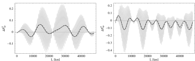
Figure 4: The same as in Fig. 4 except that the densities are $0$ and $6.4\;{\rm g/cm^{3}}$ and $E=0.5\;{\rm GeV}$. The grey curves are analytical results, whereas the black solid and dashed curves show the results averaged over fast oscillations of the analytical and numerical calculations, respectively. The figure has been taken from Ref. [1].

The left plot uses the same parameter values as in Fig. 3a of P.M. Fishbane and P. Kaus [2], whereas the right plot uses larger values of $\theta_{13}$ and $\Delta m_{21}^{2}$.

What about T violation in future terrestrial neutrino oscillation experiments including neutrino factory experiments? Will it give rise to sizeable effects that are measurable? We studied several different experimental setups for a neutrino factory with a beam energy of 50 GeV. Furthermore, we assumed $2\cdot 10^{21}$ muon decays and a detector mass of 40 kton. (See Ref. [1] for further details.) We investigated two different two-layer matter density profiles with densities $1\;{\rm g/cm}^{3}$, $3\;{\rm g/cm}^{3}$ and $3\;{\rm g/cm}^{3}$, $3.3\;{\rm g/cm}^{3}$, respectively. The first one could correspond to a sea-earth scenario and the second one to a very long baseline experiment in which there should be density perturbations. We simulated these scenarios and performed fits to the obtained event rates. In addition, we compared these simulations for symmetrized versions of the corresponding matter density profiles. The symmetrized matter density profiles are modeled by replacing the transition probabilities with the symmetrized ones:

$$P_{S}=\frac{1}{2}\left(P_{\rm dir}+P_{\rm rev}\right),$$ (5)

where $P_{\rm dir}$ and $P_{\rm rev}$ are the transition probabilities originating from the neutrino propagation in the (direct) matter density profile and the “reverse” matter density profile, respectively. Thus, the simulations are only sensitive to errors induced by the asymmetry of the matter density profile. The difference of the minimal values of the $\chi^{2}$ functions for the asymmetric and symmetrized matter density profiles is a measure of matter-induced T violation.

Our simulations show that the T-violating effects can be “quite sizeable” for the sea-earth matter density profile; however, only for $L\gtrsim 1000\;{\rm km}$, which cannot be realized on Earth. The qualitative statements of the simulations do not change very much if one changes the value of $\delta_{CP}$ in the fits. For the matter density profile with 10% density perturbations, the matter-induced T-violating effects are small for any baseline.

4 Summary and conclusions

In summary, approximative analytical formulas for the T-odd probability differences $\Delta P^{T}_{\alpha\beta}$ for an arbitrary matter density profile have been derived using perturbation theory.

Our main conclusions are the following:

• T-violating effects can be considered as a measure of genuine three-flavorness.

• For terrestial experiments matter-induced T-violating effects can safely be ignored.

• Asymmetric matter effects cannot hinder the determination of the fundamental CP and T-violating phase $\delta_{CP}$ in long baseline experiments.

- [1] E. Akhmedov, P. Huber, M. Lindner and T. Ohlsson, T violation in neutrino oscillations in matter, Nucl. Phys. B 608 (2001) 394 [hep-ph/0105029].
- [2] P.M. Fishbane and P. Kaus, Neutrino propagation in matter and a CP-violating phase, Phys. Lett. B 506 (2001) 275 [hep-ph/0012088].
- [3] Examples of works done during the last year: H. Yokomakura, K. Kimura and A. Takamura, Matter enhancement of T violation in neutrino oscillation, Phys. Lett. B 496 (2000) 175 [hep-ph/0009141]; S.J. Parke and T.J. Weiler, Optimizing T-violating effects for neutrino oscillations in matter, Phys. Lett. B 501 (2001) 106 [hep-ph/0011247]; T. Miura, E. Takasugi, Y. Kuno and M. Yoshimura, The matter effect to T violation at a neutrino factory, Phys. Rev. D 64 (2001) 013002 [hep-ph/0102111]; J. Pinney and O. Yasuda, Correlations of errors in measurements of CP violation at neutrino factories, hep-ph/0105087; M.C. Gonzalez-Garcia, Y. Grossman, A. Gusso and Y. Nir, New CP violation in neutrino oscillations, hep-ph/0105159; T. Miura, T. Shindou, E. Takasugi and M. Yoshimura, The matter fluctuation effect to T violation at a neutrino factory, hep-ph/0106086; T. Ota, J. Sato and Y. Kuno, Search for T violation in neutrino oscillations with the use of muon polarization at a neutrino factory, hep-ph/0107007; M. Fukugita and M. Tanimoto, Lepton flavor mixing matrix and CP violation from neutrino oscillation experiments, Phys. Lett. B (to be published) [hep-ph/0107082]; M. Lindner, Matter effects and CP violation at neutrino factories, Nucl. Phys. B (Proc. Suppl.) 100 (2001) 207.
- [4] P.I. Krastev and S.T. Petcov, Resonance amplification and T violation effects in three neutrino oscillations in the Earth, Phys. Lett. B 205 (1988) 84.
- [5] C. Jarlskog, A basis independent formulation of the connection between quark mass matrices, CP violation, and experiment, Z. Phys. C 29 (1985) 491; Commutator of the quark mass matrices in the standard electroweak model and a measure of maximal CP violation, Phys. Rev. Lett. 55 (1985) 1039.