Probing neutrino non–standard interactions
with atmospheric neutrino data

Abstract

We have reconsidered the atmospheric neutrino anomaly in light of the 1289-day data from Super–Kamiokande contained events and from Super–Kamiokande and MACRO up-going muons. We have reanalysed the proposed solution to the atmospheric neutrino anomaly in terms of non–standard neutrino–matter interactions (NSI) as well as the standard $\nu_{\mu}\to\nu_{\tau}$ oscillations (OSC). Our statistical analysis shows that a pure NSI mechanism is now ruled out at 99%, while the standard $\nu_{\mu}\to\nu_{\tau}$ OSC mechanism provides a quite remarkably good description of the anomaly. We therefore study an extended mechanism of neutrino propagation which combines both oscillation and non–standard neutrino–matter interactions, in order to derive limits on flavour–changing (FC) and non–universal (NU) neutrino interactions. We obtain that the off-diagonal flavour–changing neutrino parameter $\varepsilon$ and the diagonal non–universality neutrino parameter $\varepsilon^{\prime}$ are confined to $-0.05<\varepsilon<0.04$ and $|\varepsilon^{\prime}|<0.17$ at 99% CL. These limits are model independent and they are obtained from pure neutrino–physics processes. The stability of the neutrino oscillation solution to the atmospheric neutrino anomaly against the presence of non–standard neutrino interactions establishes the robustness of the near-maximal atmospheric mixing and massive–neutrino hypothesis. The best agreement with the data is obtained for $\Delta m^{2}=2.4\times 10^{-3}~{}\text{eV}^{2}$, $\sin^{2}(2\theta)=0.99$, $\varepsilon=-9.1\times 10^{-3}$ and $\varepsilon^{\prime}=-1.9\times 10^{-3}$, although the $\chi^{2}$ function is quite flat in the $\varepsilon$ and $\varepsilon^{\prime}$ directions for $\varepsilon,\varepsilon^{\prime}\to 0$. A revised analysis which takes into account the new 1489-day Super–Kamiokande and final MACRO data is presented in the appendix; the determination of $\Delta m^{2}$ and $\theta$ is essentially unaffected by the inclusion of the new data, while the bounds on $\varepsilon$ and $\varepsilon^{\prime}$ are strongly improved to $-0.03\leq\varepsilon\leq 0.02$ and $|\varepsilon^{\prime}|\leq 0.05$ at 99.73% CL.

I Introduction

The experimental data on atmospheric neutrinos SK-atm ; atm-exp ; SKconf ; Kajita:2001mr show, in the muon–type events, a clear deficit which cannot be accounted for without invoking non–standard neutrino physics. This result, together with the solar neutrino anomaly sun-exp , is very important since it constitutes a clear evidence for physics beyond the Standard Model. Altogether, the simplest joint explanation for both solar and atmospheric anomalies is the hypothesis of three-neutrino oscillations Gonzalez-Garcia:2001sq .

There are however many attempts to account for neutrino anomalies without oscillations Pakvasa:2000nt . Indeed, in addition to the simplest oscillation interpretation Gonzalez-Garcia:2000aj ; soloscother , the solar neutrino problem admits very good alternative explanations, for example based on transition magnetic moments Miranda:2001 or non–standard neutrino interactions (NSI) Bergmann:2000gp . Likewise, several such alternative mechanisms have been postulated to account for the atmospheric neutrino data such as the NSI Gonzalez-Garcia:1999hj or the neutrino decay hypotheses decay .

In contrast to the solar case, the atmospheric neutrino anomaly is so well reproduced by the $\nu_{\mu}\to\nu_{\tau}$ oscillation hypothesis (OSC) Fornengo:2000sr ; atmoscother that one can use the robustness of this interpretation so as to place stringent limits on a number of alternative mechanisms.

Among the various proposed alternative interpretations, one possibility is that the neutrinos posses non–standard interactions with matter, which were shown to provide a good description of the contained event data sample Gonzalez-Garcia:1999hj . Such non–standard interactions NSI ; Valle:1987gv ; NSIrecent can be either flavour–changing (FC) or non–universal (NU), and arise naturally in theoretical models for massive neutrinos Schechter:1980gr ; MV ; FCSU5 ; Barbieri:1995tw ; Ross:1985yg ; bergmann ; Fukugita:1988qe . This mechanism does not even require a mass for neutrinos MV ; FCSU5 although neutrino masses are expected to be present in most models Schechter:1980gr ; Barbieri:1995tw ; Ross:1985yg ; bergmann ; Fukugita:1988qe ; Gonzalez-Garcia:1989rw . It is therefore interesting to check whether the atmospheric neutrino anomaly could be ascribed, completely or partially, to non–standard neutrino–matter interactions. In Refs. Gonzalez-Garcia:1999hj ; Fornengo:2000zp ; otherFCfits the atmospheric neutrino data have been analysed in terms of a pure $\nu_{\mu}\to\nu_{\tau}$ conversion in matter due to NSI. The disappearance of $\nu_{\mu}$ from the atmospheric neutrino flux is due to interactions with matter which change the flavour of neutrinos. A complete analysis of the 52 kton-yr Super–Kamiokande data was given in Ref. Fornengo:2000zp . It included both the low–energy contained events as well as the higher energy stopping and through–going muon events, and showed that the NSI solution was acceptable, although the statistical relevance was low. Compatibility between the data and the NSI hypothesis was found to be 9.5% for relatively large values of flavour–changing and non–universality parameters.

In the present paper we will use the latest higher statistics data from Super–Kamiokande (79 kton-yr) SKconf and MACRO MACRO data in order to briefly re-analyse the atmospheric data within the oscillation hypothesis. We show that the oscillation description has a high significance, at the level of 99% for the Super–Kamiokande data, and of 95% when the MACRO through–going muons data are also added to the analysis. We then show that the new data rule out the NSI mechanism as the dominant conversion mechanism. The goodness of the fit (GOF) is now lowered to 1%. This clearly indicates that a pure NSI mechanism can not account for the atmospheric neutrino anomaly.

However, the possibility that neutrinos both posses a mass and non–standard interactions is an intriguing possibility. For example in models where neutrinos acquire a mass in see-saw type schemes the neutrino masses naturally come together with some non-diagonality of the neutrino states Schechter:1980gr . Alternatively, in supersymmetric models with breaking of R parity Ross:1985yg neutrino masses and flavour–changing interactions co-exist. This in turn can induce some amount of flavour–changing interactions. The combined mechanism of oscillations (OSC) together with NSI may be active in depleting the atmospheric $\nu_{\mu}$ flux, and therefore it can provide an alternative explanation of the deficit. Since the atmospheric neutrino anomaly is explained remarkably well by $\nu_{\mu}\to\nu_{\tau}$ oscillations, while pure NSI cannot account for the anomaly, this already indicates that NSI can be present only as a sub-dominant channel. The atmospheric neutrino data can therefore be used as a tool to set limits to the amount of NSI for neutrinos. These limits are obtained from pure neutrino–physics processes and are model independent, since they do not rely on any specific assumption on neutrino interactions. In particular they do not rely on any $SU(2)_{L}$ assumption relating the flavour–changing neutrino scattering off quarks (or electrons) to interactions which might induce anomalous tau decays Bergmann:2000pk or suffer from QCD uncertainties. In the following we will show that, from the analysis of the full set of the latest 79 kton-yr Super–Kamiokande SKconf and the MACRO data on up–going muons MACRO atmospheric neutrino data, FC and non–universal neutrino interactions are constrained to be smaller than 5% and 17% of the standard weak neutrino interaction, respectively, without any extra assumption.

The plan of the paper is the following. In Sec. II we briefly describe the theoretical origin of neutrino NSI in Earth matter. In Sec. III we briefly summarize our analysis of the atmospheric neutrino data in terms of $\nu_{\mu}\to\nu_{\tau}$ vacuum oscillations. In Sec. IV we update our analysis for the pure NSI mechanism, and we show that the latest data are able to rule it out as the dominant $\nu_{\mu}\to\nu_{\tau}$ conversion mechanism for atmospheric neutrinos. In Sec. V we therefore investigate the combined situation, where massive neutrinos not only oscillate but may also experience NSI with matter. In this section we derive limits to the NSI parameters from the atmospheric neutrino data. In Sec. VI we present our conclusions.

II Theory

Generically models of neutrino mass may lead to both oscillations and neutrino NSI in matter. Here we sketch two simple possibilities.

II.1 NSI from neutrino-mixing

The most straightforward case is when neutrino masses follow from the admixture of isosinglet neutral heavy leptons as, for example, in seesaw schemes GRS . These contain $SU(2)\otimes U(1)$ singlets with a gauge invariant Majorana mass term of the type ${M_{R}}_{ij}\nu^{c}_{i}\nu^{c}_{j}$ which breaks total lepton number symmetry. The masses of the light neutrinos are obtained by diagonalizing the mass matrix

$$\begin{bmatrix}M_{L}&D\\ D^{T}&M_{R}\end{bmatrix}$$ (1)

in the basis $\nu,\nu^{c}$, where $D$ is the standard $SU(2)\otimes U(1)$ breaking Dirac mass term, and $M_{R}=M_{R}^{T}$ is the large isosinglet Majorana mass and the $M_{L}\nu\nu$ term is an iso-triplet Schechter:1980gr . In $SO(10)$ models the first may arise from a 126 vacuum expectation value, while the latter is generally suppressed by the left-right breaking scale, $M_{L}\propto 1/M_{R}$.

In such models the structure of the associated weak currents is rather complex Schechter:1980gr . The first point to notice is that the isosinglets, presumably heavy, will mix with the ordinary isodoublet neutrinos in the charged current weak interaction. As a result, the mixing matrix describing the charged leptonic weak interaction is a rectangular matrix $K$ Schechter:1980gr which may be decomposed as

$$K=(K_{L},K_{H})$$ (2)

where $K_{L}$ and $K_{H}$ are $3\times 3$ matrices. The corresponding neutral weak interactions are described by a non-trivial matrix Schechter:1980gr

$$P=K^{\dagger}K\,.$$ (3)

In such models non–standard interactions of neutrinos with matter are of gauge origin, induced by the non-trivial structures of the weak currents. Note, however, that since the smallness of neutrino mass is due to the seesaw mechanism $M_{\nu\>eff}=M_{L}-DM_{R}^{-1}D^{T}$ the condition

$$M_{L}\ll M_{R}$$ (4)

the magnitude of neutrinos NSIs is expected to be negligible.

However the number $m$ of $SU(2)\otimes U(1)$ singlets is completely arbitrary, so that one may consider the phenomenological consequences of models with Majorana neutrinos based on any value of $m$. In this case one has $3(1+m)$ mixing angles $\theta_{ij}$ and the same number of CP violating phases $\phi_{ij}$ characterizing the neutrino mixing matrix $K$ Schechter:1980gr ; Schechter:1981gk . This number far exceeds the corresponding number of parameters describing the charged current weak interaction of quarks. The reasons are that (i) neutrinos are Majorana particles so that their mass terms are not invariant under rephasings, and (ii) the isodoublet neutrinos mix with the isosinglets. For $m\leq 3$, $3-m$ neutrinos will remain massless, while $2m$ neutrinos will acquire Majorana masses but may have non-zero NSI. For example, in a model with $m=1$ one has one light neutrino and one heavy Majorana neutrino in addition to two massless neutrinos Schechter:1980gr whose degeneracy is lifted by radiative corrections.

In contrast, the case $m>3$ may also be interesting because it allows for an elegant way to generate neutrino masses without a superheavy scale, such as in the seesaw case. This allows one to enhance the allowed magnitude of neutrino NSI strengths by avoiding constraints related to neutrino masses. As an example consider the following extension of the lepton sector of the $SU(2)\otimes U(1)$ theory: let us add a set of $two$ 2-component isosinglet neutral fermions, denoted ${\nu^{c}}_{i}$ and $S_{i}$, in each generation. In this case one can consider the $9\times 9$ mass matrix Gonzalez-Garcia:1989rw

$$\begin{bmatrix}0&D&0\\ D^{T}&0&M\\ 0&M^{T}&\mu\end{bmatrix}$$ (5)

(in the basis $\nu,\nu^{c},S$). The Majorana masses for the neutrinos are determined from

$$M_{L}=DM^{-1}\mu{M^{T}}^{-1}D^{T}\,.$$ (6)

In the limit $\mu\to 0$ the exact lepton number symmetry is recovered and will keep neutrinos strictly massless to all orders in perturbation theory, as in the Standard Model MV . The propagation of the light (massless when $\mu\to 0$) neutrinos is effectively described by an effective truncated mixing matrix $K_{L}$ which is not unitary. This may lead to oscillation effects in supernovae matter, even if neutrinos were massless Valle:1987gv ; Nunokawa:1996tg ; Grasso:1998tt . The strength of NSI is therefore unrestricted by the magnitude of neutrino masses, only by universality limits, and may be large, at the few per cent level. The phenomenological implications of these models have been widely investigated Bernabeu:1987gr ; Gonzalez-Garcia:1990fb ; Rius:1990gk ; Valle:1991pk ; Gonzalez-Garcia:1992be .

II.2 NSI from new scalar interactions

Figure 1: Diagram generating neutrino mass in supersymmetry with explicitly broken R-parity. It illustrates the co-existence of OSC and NSI mechanisms used in Eq. (24)

An alternative and elegant way to induce neutrino NSI is in the context of unified supersymmetric models as a result of supersymmetric scalar lepton non-diagonal vertices induced by renormalization group evolution FCSU5 ; Barbieri:1995tw . In the case of $SU(5)$ the NSI may exist without neutrino mass. In $SO(10)$ neutrino masses co-exist with neutrino NSI.

An alternative way to induce neutrino NSI without invoking physics at very large mass scales is in the context of some radiative models of neutrino masses Fukugita:1988qe . In such models NSI may arise from scalar interactions.

Here we focus on a more straightforward way to induce NSI based on the most general form of low-energy supersymmetry. In such models no fundamental principle precludes the possibility to violate R parity conservation Ross:1985yg explicitly by renormalizable (and hence a priori unsuppressed) operators such as the following extra $L$ violating couplings in the superpotential

$$\lambda_{ijk}L_{i}L_{j}E^{c}_{k}\,$$ (7)

$$\lambda^{\prime}_{ijk}L_{i}Q_{j}D^{c}_{k}$$ (8)

where $L,Q,E^{c}$ and $D^{c}$ are (chiral) superfields which contain the usual lepton and quark $SU(2)$ doublets and singlets, respectively, and $i,j,k$ are generation indices. The couplings in Eq. (7) give rise at low energy to the following four-fermion effective Lagrangian for neutrinos interactions with $d$-quark including

$$L_{eff}=-2\sqrt{2}G_{F}\sum_{\alpha,\beta}\xi_{\alpha\beta}\>\bar{\nu}_{L\alpha}\gamma^{\mu}\nu_{L\beta}\>\bar{d}_{R}\gamma^{\mu}{d}_{R}\>\>\>\alpha,\beta=e,\mu,\tau\,,$$ (9)

where the parameters $\xi_{\alpha\beta}$ represent the strength of the effective interactions normalized to the Fermi constant $G_{F}$. One can identify explicitly, for example, the following non–standard flavour–conserving NSI couplings

$$\xi_{\mu\mu} =\sum_{j}\frac{|\lambda^{\prime}_{2j1}|^{2}}{4\sqrt{2}G_{F}m^{2}_{\tilde{q}_{jL}}}\,,$$ (10)

$$\xi_{\tau\tau} =\sum_{j}\frac{|\lambda^{\prime}_{3j1}|^{2}}{4\sqrt{2}G_{F}m^{2}_{\tilde{q}_{jL}}}\,,$$ (11)

and the FC coupling

$$\xi_{\mu\tau}=\sum_{j}\frac{\lambda^{\prime}_{3j1}\lambda^{\prime}_{2j1}}{4\sqrt{2}G_{F}m^{2}_{\tilde{q}_{jL}}}$$ (12)

where $m_{\tilde{q}_{jL}}$ are the masses of the exchanged squarks and $j=1,2,3$ denotes $\tilde{d}_{L},\tilde{s}_{L},\tilde{b}_{L}$, respectively. Likewise, one can identify the corresponding flavour–changing NSI. The existence of effective neutral current interactions contributing to the neutrino scattering off $d$ quarks in matter, provides new flavour–conserving as well as flavour–changing terms for the matter potentials of neutrinos. Such NSI are directly relevant for atmospheric neutrino propagation. As a final remark we note that such neutrino NSI are accompanied by non-zero neutrino masses, for example, induced by loops such as that in Fig. 1. The latter lead to vacuum oscillation (OSC) of atmospheric neutrinos. The relative importance of NSI and OSC is model-dependent. In what follows we will investigate the relative importance of NSI-induced and neutrino mass oscillation induced (OSC-induced) conversion of atmospheric neutrinos allowed by the present high statistics data.

III Vacuum oscillation hypothesis

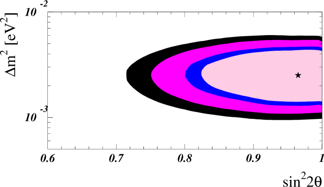
Figure 2: Allowed regions in the $\Delta m^{2}$–$\sin^{2}(2\theta)$ parameter space for the pure $\nu_{\mu}\to\nu_{\tau}$ oscillation mechanism. The shaded areas refer to the 90%, 95%, 99% and 99.73% CL with 2 parameters. The best fit point is indicated by a star. Both Super–Kamiokande and MACRO data have been included.

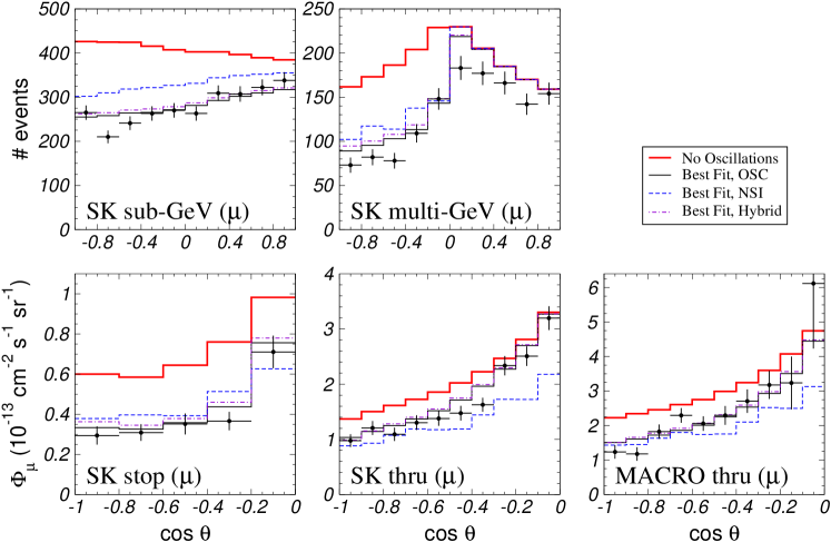
Figure 3: Zenith-angle distributions for the Super–Kamiokande and MACRO data sets, together with our predictions in the absence of oscillation (thick solid line) and the predictions for the best fit points for each data set in the different $\nu_{\mu}\to\nu_{\tau}$ transition channels: pure oscillation (thin solid line), pure NSI (dashed line) and the hybrid oscillation + NSI mechanism (dot-dashed line). The errors displayed in the experimental points are statistical only.

		$\nu_{\mu}\to\nu_{\tau}$ oscillations				NSI hypothesis
Data Set	d.o.f.	$\Delta m^{2}~{}[\text{eV}^{2}]$	$\sin^{2}(2\theta)$	$\chi_{OSC}^{2}$	GOF	$\varepsilon$	$\varepsilon^{\prime}$	$\chi_{FC}^{2}$	GOF
SK Sub-GeV	$10-2$	$2.2\times 10^{-3}$	$1.00$	$\hphantom{0}4.1$	$84\%$	$0.196$	$0.010$	$\hphantom{0}5.1$	$75\%$
SK Multi-GeV	$10-2$	$2.1\times 10^{-3}$	$0.94$	$\hphantom{0}4.2$	$84\%$	$0.667$	$0.431$	$\hphantom{0}4.2$	$84\%$
SK Stop-$\mu$	$\hphantom{0}5-2$	$3.0\times 10^{-3}$	$0.99$	$\hphantom{0}0.7$	$88\%$	$0.697$	$0.317$	$\hphantom{0}2.5$	$48\%$
SK Thru-$\mu$	$10-2$	$6.3\times 10^{-3}$	$0.78$	$\hphantom{0}5.3$	$73\%$	$0.041$	$0.138$	$\hphantom{0}5.7$	$68\%$
MACRO	$10-2$	$1.3\times 10^{-3}$	$1.00$	$11.6$	$17\%$	$0.020$	$0.046$	$\hphantom{0}6.6$	$58\%$
SK Contained	$20-2$	$2.1\times 10^{-3}$	$1.00$	$\hphantom{0}8.8$	$96\%$	$0.667$	$0.138$	$10.9$	$90\%$
SK Upgoing	$15-2$	$3.2\times 10^{-3}$	$0.94$	$\hphantom{0}6.5$	$92\%$	$0.041$	$0.144$	$16.5$	$22\%$
SK Cont+Stop	$25-2$	$2.5\times 10^{-3}$	$0.99$	$10.0$	$99\%$	$0.697$	$0.331$	$15.3$	$88\%$
Thru-$\mu$	$20-2$	$3.0\times 10^{-3}$	$0.95$	$18.1$	$45\%$	$0.018$	$0.058$	$21.1$	$28\%$
SK	$35-2$	$2.7\times 10^{-3}$	$0.97$	$16.2$	$99\%$	$0.536$	$0.611$	$53.1$	$\hphantom{0}1\%$
SK+MACRO	$45-2$	$2.5\times 10^{-3}$	$0.96$	$28.7$	$95\%$	$0.513$	$0.667$	$67.6$	$\hphantom{0}1\%$

Table 1: Minimum $\chi^{2}$ values and best-fit points for the various atmospheric neutrino data sets considered in the analysis and for two different neutrino conversion mechanisms: pure $\nu_{\mu}\to\nu_{\tau}$ vacuum oscillation (OSC) and pure non–standard neutrino–matter interactions (NSI).

We first briefly report our updated results for the usual $\nu_{\mu}\to\nu_{\tau}$ vacuum oscillation channel. For definiteness we confine to the simplest case of two neutrinos, in which case CP is conserved in standard oscillations. The evolution of neutrinos from the production point in the atmosphere up to the detector is described by the evolution equation:

$$i\dfrac{d}{dr}\begin{pmatrix}\nu_{\mu}\\ \nu_{\tau}\end{pmatrix}={\mathbf{H}}\begin{pmatrix}\nu_{\mu}\\ \nu_{\tau}\end{pmatrix},$$ (13)

where the Hamiltonian which governs the neutrino propagation can be written as:

$${\mathbf{H}}=\begin{pmatrix}H_{\mu\mu}&H_{\mu\tau}\\ H_{\mu\tau}&H_{\tau\tau}\end{pmatrix}=\dfrac{\Delta m^{2}}{4E}{\mathbf{R}}_{\theta}\begin{pmatrix}-1&~{}0\\ \hphantom{-}0&~{}1\end{pmatrix}{\mathbf{R}}_{\theta}^{\dagger},$$ (14)

In Eq. (14) $\Delta m^{2}$ is the squared–mass difference between the two neutrino mass eigenstates and the rotation matrix $\mathbf{R}_{\theta}$ is simply given in terms of the mixing angle $\theta$ by

$$\mathbf{R}_{\theta}=\begin{pmatrix}\hphantom{-}\cos\theta&~{}\sin\theta\\ -\sin\theta&~{}\cos\theta\end{pmatrix}.$$ (15)

The oscillation probability for a neutrino which travels a path of length $L$ is therefore:

$$P_{\nu_{\mu}\to\nu_{\tau}}=P_{\bar{\nu}_{\mu}\to\bar{\nu}_{\tau}}={\sin^{2}(2\theta)}\>{\sin^{2}\left(1.27\,\frac{\Delta m^{2}L}{E_{\nu}}\right)}.$$ (16)

where $\Delta m^{2}$, $L$ and ${E_{\nu}}$ are measured in $\text{eV}^{2}$, Km and GeV, respectively.

The calculation of the event rates and the statistical analysis is performed according to Ref. Fornengo:2000sr . In the present analysis we include the full set of 79 kton-yr Super–Kamiokande data SKconf and the latest MACRO data on upgoing muons MACRO . The results of the fits are shown in Table 1: the best fit point is $\Delta m^{2}=2.7\times 10^{-3}~{}\text{eV}^{2}$ and $\sin^{2}2\theta=0.97$ with a GOF of 99% when only Super–Kamiokande data are considered. The inclusion of MACRO lowers slightly the GOF to 95% but practically does not move the best fit point, which in this case is $\Delta m^{2}=2.5\times 10^{-3}~{}\text{eV}^{2}$ and $\sin^{2}2\theta=0.96$.

Fig. 2 shows the allowed region in the plane $(\sin^{2}2\theta,\Delta m^{2})$, and Fig. 3 reports the angular distributions of the Super–Kamiokande data sets and the same distributions calculated for the best fit point. The agreement between the data and the calculated rates in presence of oscillation is remarkable, for each data sample. The same occurs also for the MACRO data set.

From this analysis we can conclude that the $\nu_{\mu}\to\nu_{\tau}$ oscillation hypothesis represents a remarkably good explanation of the atmospheric neutrino anomaly (see also Refs. Fornengo:2000sr ; atmoscother ).

IV Non–standard neutrino interactions

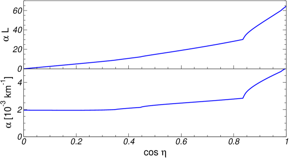
Figure 4: Function $\alpha$ of Eq. (23) and the relevant product $(\alpha L)$ which enters in the pure NSI transition probability of Eq. (22), plotted as a function of the cosine of the Earth’s zenith angle $\eta$.

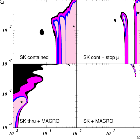
Figure 5: Allowed regions in the $\varepsilon$–$\varepsilon^{\prime}$ parameter space for the pure $\nu_{\mu}\to\nu_{\tau}$ NSI mechanism and for different sets of experimental data. The shaded areas refer to the 90%, 95%, 99% and 99.73% CL with 2 parameters. For each panel, the best fit point is indicated by a star.

Let us re-analyze the interpretation of the atmospheric neutrino anomaly in terms of pure non–standard interactions of neutrinos with matter Gonzalez-Garcia:1999hj ; Fornengo:2000zp ; otherFCfits . In this case, neutrinos are assumed to be massless and the $\nu_{\mu}\to\nu_{\tau}$ conversion is due to some NSI with the matter which composes the mantle and the core of the Earth. The evolution Hamiltonian can be written as Gonzalez-Garcia:1999hj ; Fornengo:2000zp :

$${\mathbf{H}}=\pm\sqrt{2}\,G_{F}N_{f}(r)\begin{pmatrix}0&\varepsilon_{\nu}\\ \varepsilon_{\nu}&\varepsilon^{\prime}_{\nu}\end{pmatrix},$$ (17)

where the sign $+$ ($-$) holds for neutrinos (antineutrinos) and $\varepsilon_{\nu}$ and $\varepsilon^{\prime}_{\nu}$ parametrize the deviation from standard neutrino interactions: $\sqrt{2}\,G_{F}N_{f}(r)\varepsilon_{\nu}$ is the forward scattering amplitude of the FC process $\nu_{\mu}+f\to\nu_{\tau}+f$ and $\sqrt{2}\,G_{F}N_{f}(r)\varepsilon^{\prime}_{\nu}$ represents the difference between the $\nu_{\tau}+f$ and the $\nu_{\mu}+f$ elastic forward scattering amplitudes. The quantity $N_{f}(r)$ is the number density of the fermion $f$ along the path $r$ of the neutrinos propagating in the Earth. To conform to the analyses of Ref. Gonzalez-Garcia:1999hj , we set our normalization on these parameters by considering that the relevant neutrino interaction in the Earth occurs only with down–type quarks.

In general, an equation analogous to Eq. (17) holds for anti-neutrinos, with parameters $\varepsilon_{\bar{\nu}}$ and $\varepsilon^{\prime}_{\bar{\nu}}$. For the sake of simplicity, we will assume here and in the following $\varepsilon_{\nu}=\varepsilon_{\bar{\nu}}\equiv\varepsilon$ and $\varepsilon^{\prime}_{\nu}=\varepsilon^{\prime}_{\bar{\nu}}\equiv\varepsilon^{\prime}$. It is therefore useful to introduce the following variables $(F,\varphi)$ instead of $(\varepsilon,\varepsilon^{\prime})$:

$$\varepsilon =F\sin(2\varphi),$$ (18)

$$\frac{\varepsilon^{\prime}}{2} =F\cos(2\varphi),$$

or, equivalently:

$$F =\sqrt{{\varepsilon^{\prime}}^{2}/4+\varepsilon^{2}}\,,$$ (19)

$$\varphi =\frac{1}{2}\arctan\left(\frac{\varepsilon}{\varepsilon^{\prime}/2}\right),$$

With the use of the variables $F$ and $\theta$, the evolution Hamiltonian Eq. (17) can be cast in a form which is analogous to the standard oscillation one:

$${\mathbf{H}}=\pm\sqrt{2}\,G_{F}N_{f}(r)\,F\,{\mathbf{R}}_{\varphi}\begin{pmatrix}-1&~{}0\\ \hphantom{-}0&~{}1\end{pmatrix}{\mathbf{R}}_{\varphi}^{\dagger},$$ (20)

where ${\mathbf{R}}_{\varphi}$ assumes the structure of a usual rotation matrix with angle $\varphi$:

$${\mathbf{R}}_{\varphi}=\begin{pmatrix}\hphantom{-}\cos\varphi&~{}\sin\varphi\\ -\sin\varphi&~{}\cos\varphi\end{pmatrix}.$$ (21)

The transition probabilities of $\nu_{\mu}\to\nu_{\tau}$ ($\bar{\nu}_{\mu}\to\bar{\nu}_{\tau}$) are obtained by integrating Eq. (20) along the neutrino trajectory inside the Earth. For the Earth’s density profile we employ the distribution given in PREM and a realistic chemical composition with proton/nucleon ratio 0.497 in the mantle and 0.468 in the core BK . Although the integration is performed numerically, the transition probability can be written exactly in a simple analytical form as

$$P_{\nu_{\mu}\to\nu_{\tau}}=P_{\bar{\nu}_{\mu}\to\bar{\nu}_{\tau}}={\sin^{2}\left(2\varphi\right)}\>{\sin^{2}\left(\alpha F\,L\right)},$$ (22)

where

$$\alpha=\sqrt{2}G_{F}\left<N_{f}\right>$$ (23)

and $\left<N_{f}\right>$ is the mean value of $N_{f}(r)$ along the neutrino path. Note that the analytical form in Eq. (22) holds exactly despite the fact that the number density $N_{f}(r)$ varies along the path. The quantity $\alpha$ and the relevant product $\alpha L$ which enters the transition probability in Eq. (22) are plotted in Fig. 4 as a function of the zenith angle $\eta$ and calculated for the Earth’s profile quoted above. From Fig. 4 it is clear the sharp change from the mantle to the core densities which occurs for $\cos\eta\sim 0.84$. Notice that the transition probability $P_{\nu_{\mu}\to\nu_{\tau}}$ ($P_{\bar{\nu}_{\mu}\to\bar{\nu}_{\tau}}$) is formally the same as the expression for vacuum oscillation Eq. (16) with the angle $\varphi$ playing a role of mixing angle analogous to the angle $\theta$ for vacuum oscillations. In the other hand, in the factor which depends on the neutrino path $L$, the parameter $F$ formally replaces $\Delta m^{2}$. However, in contrast to the oscillation case, there is no energy dependence in the case of NSI Gonzalez-Garcia:1999hj ; Fornengo:2000zp ; otherFCfits .

The result of the fits to the Super–Kamiokande and MACRO data are reported in Fig. 5 and again in Table 1. As already discussed in Ref. Gonzalez-Garcia:1999hj , the NSI mechanism properly accounts for each Super–Kamiokande data set separately, as well as the MACRO upgoing muons data. Moreover it succeeds in reconciling together the sub-GeV, multi-GeV and stopping muons data sets. However, the NSI cannot account at the same time also for the through-going muons events, mainly because the NSI mechanism provides an energy independent conversion probability, while the upgoing muon events, which are originated by higher energy neutrinos, require a suppression which is smaller than the one required by the other data sets Gonzalez-Garcia:1999hj ; Fornengo:2000zp ; otherFCfits . This effect is clearly visible in two ways. First, from Fig. 5, where we can see that the allowed regions for SK contained + stopping-$\mu$ events (upper-right panel) and for SK + MACRO through-going $\mu$ events (lower-left panel) are completely disjoint even at the 99.73% CL. In addition, from the angular distribution of the rates shown in Fig. 3, where the angular distribution for upgoing muons calculated for the best fit point of the pure NSI mechanism clearly shows too a strong suppression, especially for horizontal events. The global analysis of Super–Kamiokande and MACRO data has a very low GOF, only 1%: this now allows us to rule out at 99% the pure NSI mechanism as a possible explanation of the atmospheric neutrino anomaly.

V Combining the OSC and NSI mechanisms

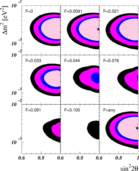
Figure 6: Allowed regions in the $\Delta m^{2}$–$\sin^{2}(2\theta)$ parameter space for the hybrid OSC + NSI mechanism. In each panel, the value of the NSI parameter $F$ is fixed, while the other NSI parameter $\varphi$ is integrated out. The last panel shows the allowed region when both $F$ and $\varphi$ are integrated out. The shaded areas refer to the 90%, 95%, 99% and 99.73% CL with 3 parameters, and the best fit point is indicated by a star. Both Super–Kamiokande and MACRO data have been included.

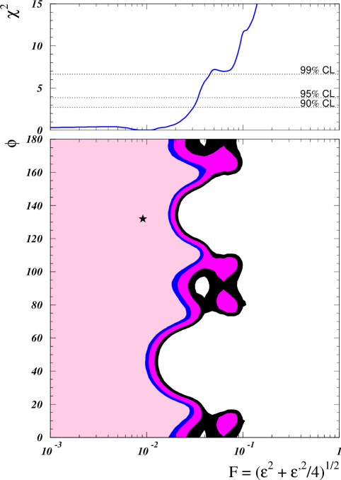
Figure 7: Allowed regions in the $F$–$\varphi$ parameter space for the hybrid OSC + NSI mechanism. The parameters $\Delta m^{2}$ and $\sin^{2}(2\theta)$ are integrated out. The shaded areas refer to the 90%, 95%, 99% and 99.73% CL with 2 parameters, and the best fit point is indicated by a star. The top panel shows the behaviour of the $\chi^{2}$ as a function of the NSI parameter $F$ when $\varphi$ is also integrated out. Both Super–Kamiokande and MACRO data have been included.

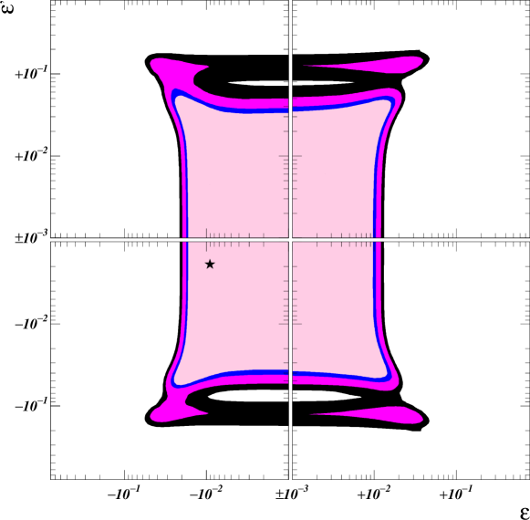
Figure 8: Allowed regions in the $\varepsilon$–$\varepsilon^{\prime}$ parameter space for the hybrid OSC + NSI mechanism. The parameters $\Delta m^{2}$ and $\sin^{2}(2\theta)$ are integrated out. Notice that both positive and negative values of $\varepsilon$ and $\varepsilon^{\prime}$ are shown. The shaded areas refer to the 90%, 95%, 99% and 99.73% CL with 2 parameters, and the best fit point is indicated by a star. Both Super–Kamiokande and MACRO data have been included.

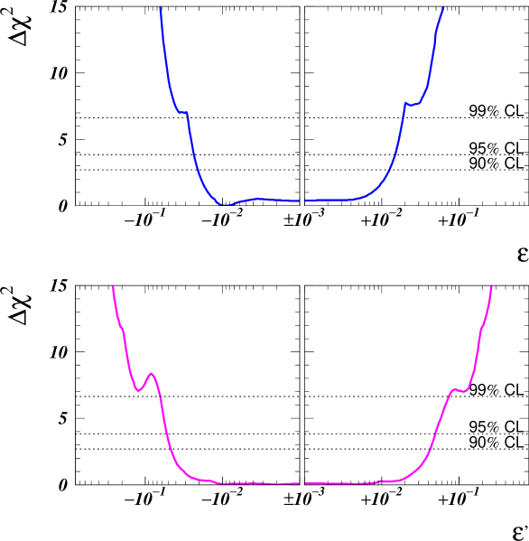
Figure 9: Behaviour of the $\chi^{2}$ as a function of the flavour–changing parameter $\varepsilon$ (top panel) and of the non–universal neutrino-interactions parameter $\varepsilon^{\prime}$ (bottom panel), for the hybrid OSC + NSI mechanism. In each panel both the oscillation parameters ($\sin^{2}(2\theta)$ and $\Delta m^{2}$) and the undisplayed NSI parameter ($\varepsilon^{\prime}$ in the top panel and $\varepsilon$ in the bottom one) are integrated out. Notice that both positive and negative values of $\varepsilon$ and $\varepsilon^{\prime}$ are shown.

Let us now consider the possibility that neutrinos are massive and moreover posses non–standard interactions with matter. As mentioned in Sec. II, this may be regarded as generic in a large class of theoretical models. In this case, their propagation inside the Earth is governed by the following Hamiltonian

$${\mathbf{H}}=\dfrac{\Delta m^{2}}{4E}{\mathbf{R}}_{\theta}\begin{pmatrix}-1&~{}0\\ \hphantom{-}0&~{}1\end{pmatrix}{\mathbf{R}}_{\theta}^{\dagger}\pm\sqrt{2}\,G_{F}N_{f}(r)\,F\,{\mathbf{R}}_{\varphi}\begin{pmatrix}-1&~{}0\\ \hphantom{-}0&~{}1\end{pmatrix}{\mathbf{R}}_{\varphi}^{\dagger},$$ (24)

where $\mathbf{R}_{\theta}$ and ${\mathbf{R}}_{\varphi}$ are the mixing matrices defined in Eqs. (15) and (21), respectively. The NSI term in the Hamiltonian has an effect which is analogous to the presence of the effective potentials for the propagation in matter of massive neutrinos, a situation which leads to the MSW oscillation mechanism MSW . Also in the case of Eq. (24) neutrinos can experience matter–induced oscillations, due to the fact that $\nu_{\mu}$’s and $\nu_{\tau}$’s can have both flavour–changing and non–universal interaction with the Earth matter.

Since the Earth’s matter profile function $N_{f}(r)$ is not constant along the neutrino propagation trajectories, the Hamiltonian matrices calculated at different points inside the Earth do not commute. This leads to a non trivial evolution for the neutrinos in the Earth and a numerical integration of the Eq. (13) with the Hamiltonian of Eq. (24) is needed in order to calculate the neutrino and anti-neutrino transition probabilities $P_{\nu_{\mu}\to\nu_{\tau}}$ and $P_{\bar{\nu}_{\mu}\to\bar{\nu}_{\tau}}$.

The transition mechanism depends on four independent parameters: the neutrino squared–mass difference $\Delta m^{2}$, the neutrino mixing angle $\theta$, the FC parameter $\varepsilon$ and the NU parameter $\varepsilon^{\prime}$ (or, alternatively, the $F$ and $\varphi$ parameters for the NSI sector). In our analysis we will use the $F$ and $\varphi$ parameters, which prove to be more useful, and then express the results, which we will obtain for these two parameters, in terms of the $\varepsilon$ and $\varepsilon^{\prime}$ parameters, which have a more physical meaning.

As a first step, we can use the symmetries of the Hamiltonian in order to properly define the intervals of variation of the parameters. Since $\mathbf{H}$ in Eq. (24) is real and symmetric, the transition probabilities are invariant under the following transformations:

• $\theta\to\theta+\pi$,

• $\varphi\to\varphi+\pi$,

• $\Delta m^{2}\to-\Delta m^{2}\quad\text{and}\quad\theta\to\theta+\pi/2$,

• $F\to-F\quad\text{and}\quad\varphi\to\varphi+\pi/2$.

Under any of the above transformations the Hamiltonian remains invariant. Moreover even if the overall sign of the Hamiltonian changes this will have no effect in the calculation of $P_{\nu_{\mu}\to\nu_{\tau}}$ and $P_{\bar{\nu}_{\mu}\to\bar{\nu}_{\tau}}$:

• $\theta\to\theta+\pi/2\quad\text{and}\quad\varphi\to\varphi+\pi/2\quad(\text{or:}\quad\varepsilon\to-\varepsilon\quad\text{and}\quad\varepsilon^{\prime}\to-\varepsilon^{\prime})$.

Finally, if the sign of the non-diagonal entries in the Hamiltonian changes, again there is no effect in the neutrino/anti-neutrino conversion probabilities:

• $\theta\to-\theta\quad\text{and}\quad\varphi\to-\varphi\quad(\text{or:}\quad\varepsilon\to-\varepsilon)$.

The above set of invariance transformations allows us to define the ranges of variation of the four parameters as follows:

$$(a) 0\leq\theta\leq\pi/4\,,$$ (25)

$$(b) 0\leq\varphi\leq\pi\,,$$

$$(c) \Delta m^{2}\geq 0\,,$$

$$(d) F\geq 0\,.$$

Notice that, in contrast with the MSW mechanism, it is possible here, without loss of generality, to constrain both the mixing angle $\theta$ inside the $[0,\pi/4]$ interval keeping $\Delta m^{2}$ positive. There is no “dark side” deGouvea:2000cq in the parameter space for this mechanism. In our analysis we will adopt the set of conditions of Eq. (25), implying that the neutrino squared–mass difference and mixing angle are confined to the same intervals as in the standard $\nu_{\mu}\to\nu_{\tau}$ oscillation case, while the NSI parameters $\varepsilon$ and $\varepsilon^{\prime}$ can assume independently both positive and negative values. We will actually find that the best fit point occurs for negative $\varepsilon$ and $\varepsilon^{\prime}$.

Let us turn now to the analysis of the data and the presentation of the results. Here we perform a global fit of the Super–Kamiokande data sets and of the MACRO upgoing muon flux data in terms of the four parameters of the present combined OSC + NSI mechanism. As we have already seen in the previous sections, pure oscillation provides a remarkably good fit to the data, while the pure NSI mechanism is not able to reconcile the anomaly observed in the upgoing muon sample with that seen in the contained event sample. This already indicates that, when combining the two mechanisms of $\nu_{\mu}\to\nu_{\tau}$ transition, the oscillation will play the role of leading mechanism, while the NSI could be present at a subdominant level.

As a first result, we quote the best fit solution: $\Delta m^{2}=2.4\times 10^{-3}~{}\text{eV}^{2}$, $\sin^{2}(2\theta)=0.99$, $\varepsilon=-9.1\times 10^{-3}$ and $\varepsilon^{\prime}=-1.9\times 10^{-3}$. The goodness of the fit is 94% ($45-4$ degrees of freedom). For the $\Delta m^{2}$ and $\sin^{2}(2\theta)$ parameters, the best fit is very close to the best fit solution for pure oscillation (see Table 1). This is a first indication that the oscillation mechanism is stable under the perturbation introduced by the additional NSI mechanism. It is interesting to observe that a small amount of FC could be present, at the level of less than a percent, while $\nu_{\mu}$ and $\nu_{\tau}$ interactions are likely to be universal. Moreover, the $\chi^{2}$ function is quite flat in the $\varepsilon$ and $\varepsilon^{\prime}$ directions for $\varepsilon,\varepsilon^{\prime}\to 0$.

We also display the effect of the NSI mechanism on the determination of the oscillation parameters by showing the result of the analysis in the $\Delta m^{2}$ and $\sin^{2}(2\theta)$ plane, for fixed values of the NSI parameters.

Fig. 6 shows the dependence of the allowed region in the $\Delta m^{2}$ and $\sin^{2}(2\theta)$ plane for fixed values of the NSI parameters, in particular for fixed values of $F$ irrespective of the value of $\varphi$, which is “integrated out”. Note that for $F\lesssim 0.02$ the allowed region is almost unaffected by the presence of NSI. For larger values the quality of the fit gets rapidly worse, however the position of the best fit point in the plane $(\sin^{2}(2\theta),\Delta m^{2})$ remains extremely stable. For $F\gtrsim 0.1$ the 99% CL allowed region finally disappears. The last panel of Fig. 6 shows the allowed region when both $F$ and $\varphi$ are integrated out. The region obtained is in agreement with the one obtained for pure oscillation case. We can therefore conclude that the determination of the oscillation parameters $\Delta m^{2}$ and $\sin^{2}(2\theta)$ is very stable under the effect of non–standard neutrino–matter interactions.

We can now look at the results from the point of view of the NSI parameters. This will allow us to set bounds on the maximum allowed level of neutrino NSI. Fig. 7 shows the behaviour of the $\chi^{2}$ as a function of the $F$ parameter, and the allowed region in the $F$ and $\varphi$ parameter space with $\Delta m^{2}$ and $\sin^{2}(2\theta)$ integrated out. From the lower panel we see that the $F$ parameter is constrained by the data to values smaller than $\sim 0.09$ at 99% CL, while the quantity $\varphi$ is not constrained to any specific interval. When $\varphi$ is also integrated out (upper panel of Fig. 7) the number of free parameters is reduced to $1$, and the upper bound on $F$ improves to $\sim 0.05$.

Looking at Fig. 7 and taking into account the definition of $F$ and $\varphi$ in terms of $\varepsilon$ and $\varepsilon^{\prime}$ given in Eq. (19), we see that the data constrain the maximum amount of FC and NU which is allowed (from $F$), but they do not fix their relative amount (through $\varphi$). This information can be conveniently translated in the $\varepsilon$ and $\varepsilon^{\prime}$ plane, as we show in Fig. 8: at 99% CL, the flavour–changing parameter $\varepsilon$ is confined to $-0.05<\varepsilon<0.04$, while the non–universality parameter is bounded to $|\varepsilon^{\prime}|<0.17$. These are the strongest bounds which can be imposed simultaneously on both FC and NU neutrino–matter interactions, but it is also interesting to look at the separate behaviour of the $\chi^{2}$ with respect to either FC or NU-type neutrino NSI when the other type of interaction is also integrated out. This is illustrated in Fig. 9, where we see that the bounds on $\varepsilon$ and $\varepsilon^{\prime}$ – now calculated with only $1$ degree of freedom – are improved to $-0.03<\varepsilon<0.02$ and $|\varepsilon^{\prime}|<0.07$. We also notice that the $\chi^{2}$ function is more shallow for $\varepsilon^{\prime}$ than for $\varepsilon$, indicating that the bound on FC interactions is more stringent than the one on NU interactions.

This is the main result of our analysis, since it provides limits to non–standard neutrino interactions which are truly model independent, since they are obtained from pure neutrino–physics processes. In particular they do not rely on any relation between neutrinos and charged lepton interactions. Therefore our bounds are totally complementary to what may be derived on the basis of conventional accelerator experiments Groom:2000in . Note that although the above bounds of neutrino-matter NSI were obtained simply on the basis of the quality of present atmospheric data, they are almost comparable in sensitivity to the capabilities of a future neutrino factory based on intense neutrino beams from a muon storage ring Gago:2001xg .

VI Conclusions

In this paper we have analysed the most recent and large statistic data on atmospheric neutrinos (Super–Kamiokande and MACRO) in terms of three different mechanisms: (i) pure OSC $\nu_{\mu}\to\nu_{\tau}$ oscillation; (ii) pure NSI $\nu_{\mu}\to\nu_{\tau}$ transition due to non–standard neutrino–matter interactions (flavour–changing and non–universal); (iii) hybrid OSC + NSI $\nu_{\mu}\to\nu_{\tau}$ transition induced by the presence of both oscillation and non–standard interactions.

The pure oscillation case, as is well known, provides a remarkably good fit to the experimental data, and it can be considered the best and most natural explanation of the atmospheric neutrino anomaly. In this updated analysis, we obtain the best fit solution for $\Delta m^{2}=2.5\times 10^{-3}~{}\text{eV}^{2}$ and $\sin^{2}2\theta=0.96$, with a goodness-of-fit of 95% (Super–Kamiokande and MACRO combined).

In contrast, the pure NSI mechanism, mainly due to its lack of energy dependence in the transition probability, is not able to reproduce the measured rates and angular distributions of the full data sample because it spans about three orders of magnitude in energy. The data clearly show the presence of an up–down asymmetry and some energy dependence. With the increased statistics of the data presently available it is now possible to rule out this mechanism at 99% as a possible explanation of the atmospheric neutrino data.

We have therefore investigated a more general situation: the possibility that massive neutrinos also possess some amount of flavour–changing interactions with matter, as well as some difference in the interactions between $\nu_{\mu}$’s and $\nu_{\tau}$’s. The global analysis of the Super–Kamiokande and MACRO data shows that the oscillation hypothesis is very stable against the possible additional presence of such non–standard neutrino interactions. The best fit point is obtained for $\Delta m^{2}=2.4\times 10^{-3}~{}\text{eV}^{2}$, $\sin^{2}(2\theta)=0.99$, $\varepsilon=-9.1\cdot 10^{-3}$ and $\varepsilon^{\prime}=-1.9\times 10^{-3}$ with a goodness-of-fit of 94% ($45-4$ degrees of freedom). A small amount of FC could therefore be present, at the level of less than a percent, while $\nu_{\mu}$ and $\nu_{\tau}$ interactions are likely to be universal. In addition the $\chi^{2}$ function is rather flat in the $\varepsilon$ and $\varepsilon^{\prime}$ directions for $\varepsilon,\varepsilon^{\prime}\to 0$ and NSI can be tolerated as long as their effect in atmospheric neutrino propagation is subdominant.

From the analysis we have therefore derived bounds on the amount of flavour–changing and non–universality allowed in neutrino–matter interactions. At the 99% CL, the flavour–changing parameter $\varepsilon$ and the non–universality parameter $\varepsilon^{\prime}$ are simultaneously confined to $-0.05<\varepsilon<0.04$ and $|\varepsilon^{\prime}|<0.17$. The bounds on flavour–changing interactions is stronger than the one which applies on universality violating ones. These bounds on non–standard neutrino interactions do not rely on any assumption on the underlying particle physics model, as they are obtained from pure neutrino–physics processes. They could be somewhat improved at a future neutrino factory based on intense neutrino beams from a muon storage ring.

Note in particular that the bounds derived here imply that we can not avoid having a maximal atmospheric neutrino mixing angle $\theta$ by using NSI with non-zero $\varphi$, despite the fact that the value of $\varphi$ is essentially unrestricted. The reason for this lies in the fact that the allowed magnitude of neutrino NSI measured by $F$ is so constrained (due to the lack of energy dependence of the NSI evolution equation) that its contribution must be sub-leading. This means that a maximum atmospheric neutrino mixing angle is a solid result which must be incorporated into any acceptable particle physics model, even in the presence of exotic neutrino interactions.

*

Appendix A New super–Kamiokande and MACRO data

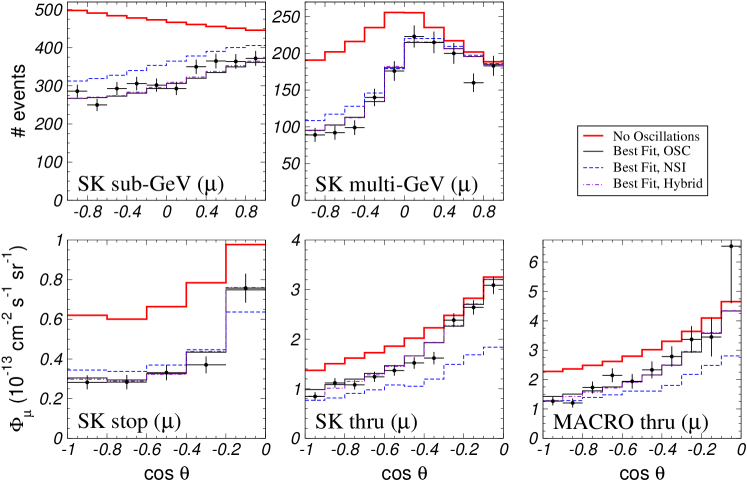
Figure 10: Same as Fig. 3, but using the latest Super–K and MACRO data. In the theoretical calculation of the expected event numbers the non-zero scattering angle between the incoming neutrino and the scattered lepton directions is now properly taken into account.

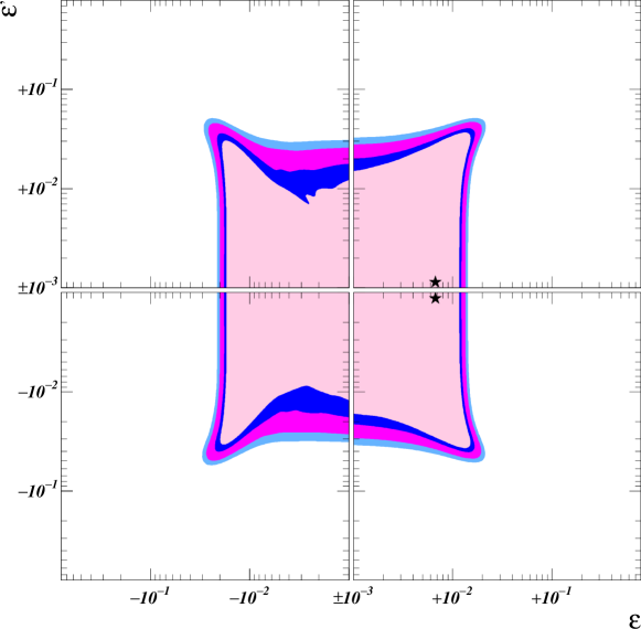
Figure 11: Allowed regions in the $\varepsilon$–$\varepsilon^{\prime}$ parameter space for the hybrid OSC + NSI mechanism, using the new Super–Kamiokande and MACRO data. The oscillation parameters $\Delta m^{2}$ and $\sin^{2}(2\theta)$ are integrated out. The shaded areas refer to the 90%, 95%, 99% and 99.73% CL with 2 parameters, and the best fit points are indicated by stars.

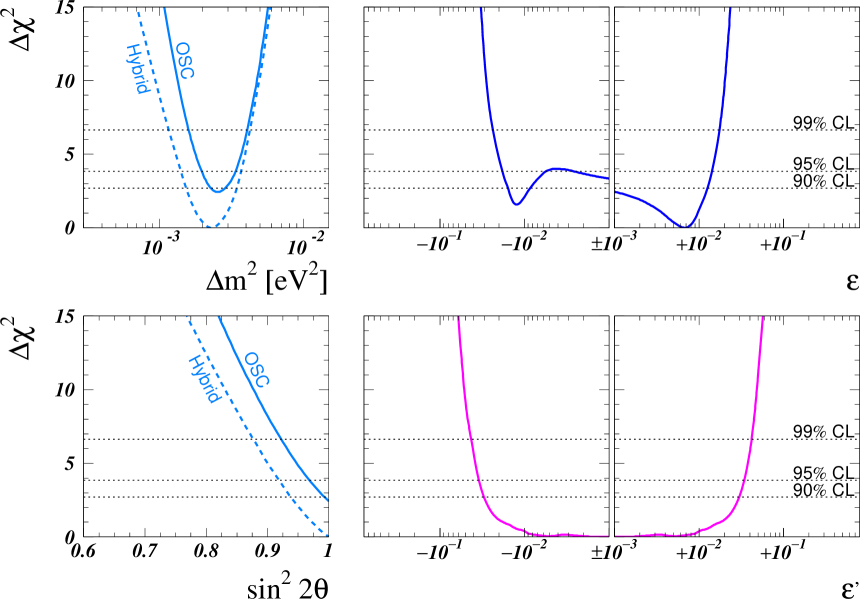
Figure 12: Behaviour of $\Delta\chi^{2}$ for the new Super–Kamiokande and MACRO data, as a function of the oscillation parameters $\Delta m^{2}$ and $\theta$ (left panels), and of the NSI parameters $\varepsilon$ and $\varepsilon^{\prime}$ (right panels). In each panel the undisplayed parameters are integrated out. In the left panels both the pure oscillations case and the hybrid OSC + NSI mechanism are displayed.

In this section (which does not appear in the published version of this paper) we present an update of the hybrid OSC + NSI analysis discussed in Sec. V. The calculation of the event rates and the statistical analysis is performed according to Ref. Maltoni:2002ni , which improves the one used so far in essentially three ways:

Experimental data.

Both the Super-Kamiokande and the MACRO collaborations have recently released new data. The Super-Kamiokande data used here correspond to 1489 days skatm-1489 , and include the $e$-like and $\mu$-like charged-current data samples of sub- and multi-GeV contained events (10 bins in zenith angle), as well as the stopping (5 angular bins) and through-going (10 angular bins) up-going muon data events. From MACRO we use the through-going muon sample presented in macro-last , divided in 10 angular bins.

Statistical analysis.

We now take advantage of the full ten-bin zenith-angle distribution for the Super-Kamiokande contained events, rather than the five-bin distribution employed previously. Therefore, we have now $65$ observables, which we fit in terms of the four relevant parameters $\Delta m^{2}$, $\theta$, $\varepsilon$ and $\varepsilon^{\prime}$.

Theoretical Monte-Carlo.

We improve the method presented in Ref. Fornengo:2000sr by properly taking into account the scattering angle between the incoming neutrino and the scattered lepton directions. This was already the case for Sub-GeV contained events, however previously we made the simplifying assumption of full neutrino-lepton collinearity in the calculation of the expected event numbers for the Multi-GeV contained and up-going-$\mu$ data samples. While this approximation is still justified for the stopping and thru-going muon samples, in the Multi-GeV sample the theoretically predicted value for down-coming $\nu_{\mu}$ is systematically higher if full collinearity is assumed, as can be clearly seen from the second panel of Fig. 3. The reason for this is that the strong suppression observed in these bins cannot be completely ascribed to the oscillation of the down-coming neutrinos (which is small due to small travel distance). Because of the non-negligible neutrino-lepton scattering angle at these Multi-GeV energies there is a sizable contribution from up-going neutrinos (with a higher conversion probability due to the longer travel distance) to the down-coming leptons. However, this problem becomes less visible when the angular information of Multi-GeV events is included in a five angular bins presentation of the data, as previously assumed Fornengo:2000sr .

Our results are summarized in Figs. 10, 11 and 12. As already found in Sec. IV using the old data set, the pure NSI solution $\Delta m^{2}=0$ gives a very poor fit, and it is completely ruled out. This occurs since the NSI mechanism is not able to reconcile the anomaly observed in the upgoing muon sample with that seen in the contained event sample, as can be clearly seen by looking at the NSI line in Figs. 3 and 10. Conversely, the pure oscillation solution $\varepsilon=\varepsilon^{\prime}=0$ is in very good agreement with the experimental data. Therefore, we can expect that, when combining the two mechanisms of $\nu_{\mu}\to\nu_{\tau}$ transition, oscillations will play the role of leading mechanism, while NSI’s can only be present at a sub-dominant level.

The global best fit point occurs at the parameter values:

$$\sin^{2}(2\theta)=1,\quad\Delta m^{2}=2.3\times 10^{-3}~{}\text{eV}^{2},\quad\varepsilon=6.7\times 10^{-3},\quad\varepsilon^{\prime}=\pm 1.1\times 10^{-3},$$ (26)

and it is interesting to note that the new data favour a small but non-vanishing component of NSI. From Fig. 10 we can see that this preference originates from the most vertical events in the the Super–Kamiokande and MACRO thru-going $\mu$ data samples, which slightly favour a stronger suppression of the neutrino signal. However, this effect is not statistically significant: the best pure oscillation solution $\varepsilon=\varepsilon^{\prime}=0$, which occurs at $\theta=45^{\circ}$ and $\Delta m^{2}=2.5\times 10^{-3}~{}\text{eV}^{2}$, exhibits a $\chi^{2}$ which is worse than the global one only by 2.4 units. The determination of the oscillation parameters $\Delta m^{2}$ and $\theta$ is very stable under the perturbation introduced by the additional NSI mechanism: from the two left panels of Fig. 12 we see that the range of $\theta$ is essentially unaffected, and the only effect of allowing for NSI is to slightly weaken the lower bound on $\Delta m^{2}$. For these parameters we derive the ranges $0.84\leq\sin^{2}(2\theta)\leq 1$ and $1.0\times 10^{-3}~{}\text{eV}^{2}\leq\Delta m^{2}\leq 4.8\times 10^{-3}~{}\text{eV}^{2}$ at 99.73% CL. The bounds on the NSI parameters derived in Sec. V are strongly improved by the inclusion of the new Super–Kamiokande data, and at 99.73% CL we now have $-0.03\leq\varepsilon\leq 0.02$ and $|\varepsilon^{\prime}|\leq 0.05$. In addition, from the right panels of Fig. 12 we see that the $\chi^{2}$ function is quite flat in the $\varepsilon^{\prime}$ directions for $\varepsilon^{\prime}\to 0$, and almost symmetric under the exchange $\varepsilon^{\prime}\to-\varepsilon^{\prime}$.

References

- (1) Y. Fukuda et al., Super-Kamiokande Coll., Phys. Rev. Lett. 81 (1998) 1562; Phys. Rev. Lett. 82, 2644 (1999)
- (2) Y. Fukuda et al., Kamiokande Coll., Phys. Lett. B 335 (1994) 237; R. Becker-Szendy et al., IMB Coll., Nucl. Phys. B (Proc. Suppl.) 38 (1995) 331; W.W.M. Allison et al., Soudan Coll., Phys. Lett. B 449 (1999) 137; M. Ambrosio et al., MACRO Coll., Phys. Lett. B 434 (1998) 451.
- (3) Super-Kamiokande presentations in winter conferences: C. McGrew in Neutrino Telescopes 2001, Venice, Italy, March 2001, to appear; T. Toshito in Moriond 2001, Les Arcs, France, March 2001, to appear.
- (4) For a review see T. Kajita and Y. Totsuka, Rev. Mod. Phys. 73 (2001) 85.
- (5) B.T. Cleveland et al., Astrophys. J. 496 (1998) 505; K.S. Hirata et al., Kamiokande Coll., Phys. Rev. Lett. 77 (1996) 1683; W. Hampel et al., GALLEX Coll., Phys. Lett. B 447 (1999) 127; D.N. Abdurashitov et al., SAGE Coll., Phys. Rev. Lett. 83 (1999) 4686; Y. Fukuda et al., Super-Kamiokande Coll., Phys. Rev. Lett. 81 (1998) 1158.
- (6) M. C. Gonzalez-Garcia, M. Maltoni, C. Pena-Garay and J. W. F. Valle, “Global three-neutrino oscillation analysis of neutrino data,” Phys. Rev. D 63 (2001) 033005 [hep-ph/0009350]. G. L. Fogli, E. Lisi, A. Marrone, D. Montanino and A. Palazzo, “Atmospheric, solar, and CHOOZ neutrinos: A global three generation analysis,” Talk given at 36th Rencontres de Moriond on Electroweak Interactions and Unified Theories, Les Arcs, France, 10-17 Mar 2001.
- (7) S. Pakvasa, Pramana 54 (2000) 65 [hep-ph/9910246].
- (8) M. C. Gonzalez-Garcia, P. C. de Holanda, C. Pena-Garay and J. W. F. Valle, Nucl. Phys. B 573 (2000) 3 [hep-ph/9906469].
- (9) V. Barger, D. Marfatia and K. Whisnant, hep-ph/0106207; G.L. Fogli et al., hep-ph/0106247; J.N. Bahcall et al., hep-ph/0106258; A. Bandyopadhyay et al., hep-ph/0106264; P. Creminelli et al., hep-ph/0102234
- (10) O. Miranda, et al Nucl. Phys. B 595 (2001) 360; J. Pulido and E. Akhmedov, Phys. Lett. B485 (2000) 178; M.M. Guzzo and H. Nunokawa, Astropart. Phys. 12 (1999) 8
- (11) S. Bergmann, M. M. Guzzo, P. C. de Holanda, P. I. Krastev and H. Nunokawa, Phys. Rev. D 62 (2000) 073001 [hep-ph/0004049].
- (12) M. C. Gonzalez-Garcia et al., Phys. Rev. Lett. 82 (1999) 3202 [hep-ph/9809531].
- (13) V. Barger, J.G. Learned, S. Pakvasa, and T.J. Weiler, Phys. Rev. Lett. 82, 2640 (1999); G.L. Fogli, E. Lisi, A. Marrone, G. Scioscia, Phys. Rev. D59, 117303 (1999). For particle physics models of unstable neutrinos see Ref. Valle:1991pk
- (14) S. Coleman, S. L. Glashow, Phys. Lett. B405, 249 (1997); S. L. Glashow, A. Halprin, P.I. Krastev , C.N. Leung, J. Pantaleone, Phys. Rev. D56, 2433 (1997).
- (15) S. Coleman, S. L. Glashow, Phys. Rev. D59, 116008 (1999).
- (16) M. Gasperini, Phys. Rev. D38, 2635 (1988); J. Pantaleone, A. Halprin, C.N. Leung, Phys. Rev. D47, 4199 (1993); A. Halprin, C.N. Leung, J. Pantaleone Phys. Rev. D53, 5365 (1996).
- (17) N. Fornengo, M. C. Gonzalez-Garcia and J. W. F. Valle, Nucl. Phys. B 580 (2000); M. C. Gonzalez-Garcia, H. Nunokawa, O. L. Peres and J. W. F. Valle, Nucl. Phys. B 543 (1999) 3; M. C. Gonzalez-Garcia, H. Nunokawa, O. L. Peres, T. Stanev and J. W. F. Valle, Phys. Rev. D 58 (1998) 033004.
- (18) R. Foot, R. R. Volkas and O. Yasuda, Phys. Rev. D58, 013006 (1998); O. Yasuda, Phys. Rev. D58, 091301 (1998); G. L. Fogli, E. Lisi, A. Marrone, G. Scioscia, Phys. Rev. D59, 03300 (1999), hep-ph/9808205; E.Kh. Akhmedov, A.Dighe, P. Lipari and A.Yu. Smirnov, Nucl. Phys. B542,3 (1999)
- (19) L. Wolfenstein, Phys. Rev. D17, 236 (1978); J. Schechter and J.W.F. Valle, Phys. Rev. D 22 (1980) 2227
- (20) J. W. F. Valle, Phys. Lett. B 199 (1987) 432.
- (21) M. Guzzo, A. Masiero and S. Petcov, Phys. Lett. B260, 154 (1991); E. Roulet, Phys. Rev. D44, 935 (1991); V. Barger, R. J. N. Phillips and K. Whisnant, Phys. Rev. D44, 1629 (1991); S. Bergmann, Nucl. Phys. B515, 363 (1998); E. Ma and P. Roy, Phys. Rev. Lett. 80, 4637 (1998).
- (22) J. Schechter and J. W. F. Valle, Phys. Rev. D 22 (1980) 2227.
- (23) R. Mohapatra, J. W. F. Valle, Phys. Rev. D34, 1642 (1986); D. Wyler and L. Wolfenstein, Nucl. Phys. B218, 205 (1983)
- (24) L. J. Hall, V. A. Kostelecky and S. Raby, Nucl. Phys. B267 415 (1986)
- (25) R. Barbieri, L. Hall and A. Strumia, Nucl. Phys. B 445, 219 (1995) [hep-ph/9501334].
- (26) L.J. Hall and M. Suzuki, Nucl. Phys. B231 (1984) 419; G.G. Ross and J.W. F. Valle, Phys. Lett. 151B (1985) 375; J. Ellis, G. Gelmini, C. Jarlskog, G.G. Ross and J.W. F. Valle, Phys. Lett. 150B (1985) 142
- (27) S. Bergmann, H.V. Klapdor-Kleingrothaus, H. Paes Phys.Rev. D 62 (2000) 113002 [hep-ph/0004048]
- (28) M. Fukugita and T. Yanagida, Phys. Lett. B 206 (1988) 93.
- (29) M. C. Gonzalez-Garcia and J. W. F. Valle, Phys. Lett. B 216 (1989) 360.
- (30) N. Fornengo, M. C. Gonzalez-Garcia and J. W. F. Valle, JHEP 0007 (2000) 006 [hep-ph/9906539].
- (31) P. Lipari and M. Lusignoli, Phys. Rev. D 60 (1999) 013003 [hep-ph/9901350]. G. L. Fogli, E. Lisi, A. Marrone and G. Scioscia, atmospheric neutrino experiment,” Phys. Rev. D 60 (1999) 053006 [hep-ph/9904248].
- (32) M. Guzzo et al., Nucl. Phys. B (Proc. Suppl.) 87 (2000) 201.
- (33) M. Spurio et al., MACRO Coll., hep-ex/0101019; B. Barish, MACRO Coll., Talk given at Neutrino 2000, 15–21 June 2000, Sudbury, Canada.
- (34) M. Hirsch, M. A. Diaz, W. Porod, J. C. Romao and J. W. F. Valle, Phys. Rev. D 62 (2000) 113008 [hep-ph/0004115]; J. C. Romao et al, Phys. Rev. D 61 (2000) 071703 [hep-ph/9907499]
- (35) S. Bergmann, Y. Grossman and D. M. Pierce, Phys. Rev. D 61 (2000) 053005 [hep-ph/9909390].
- (36) M Gell-Mann, P Ramond, R. Slansky, in Supergravity, ed. P.van Niewenhuizen and D. Freedman (North Holland, 1979); T. Yanagida, in KEK lectures, ed. O. Sawada and A. Sugamoto (KEK, 1979); R. N. Mohapatra and G. Senjanovic, Phys. Rev. Lett. 44 912 (1980).
- (37) J. Schechter and J. W. F. Valle, Phys. Rev. D 23 (1981) 1666.
- (38) H. Nunokawa, Y. Z. Qian, A. Rossi and J. W. F. Valle, Phys. Rev. D 54 (1996) 4356 [hep-ph/9605301].
- (39) D. Grasso, H. Nunokawa and J. W. F. Valle, Phys. Rev. Lett. 81 (1998) 2412 [astro-ph/9803002].
- (40) J. Bernabeu, A. Santamaria, J. Vidal, A. Mendez and J. W. F. Valle, Phys. Lett. B 187 (1987) 303.
- (41) M. C. Gonzalez-Garcia, A. Santamaria and J. W. F. Valle, Nucl. Phys. B 342 (1990) 108. M. Dittmar, A. Santamaria, M. C. Gonzalez-Garcia and J. W. F. Valle, Nucl. Phys. B 332, 1 (1990).
- (42) N. Rius and J. W. F. Valle, Phys. Lett. B 246 (1990) 249.
- (43) J. W. F. Valle, Prog. Part. Nucl. Phys. 26 (1991) 91.
- (44) M. C. Gonzalez-Garcia and J. W. F. Valle, Mod. Phys. Lett. A 7 (1992) 477. A. Ilakovac, Phys. Rev. D 62 (2000) 036010 [hep-ph/9910213].
- (45) A.M. Dziewonski and D.L. Anderson, Phys. Earth Planet. Inter. 25, 297 (1981).
- (46) J. Bahcall and P. Krastev, Phys. Rev. C56, 2839 (1997).
- (47) L. Wolfenstein, Phys. Rev. D 17, 2369 (1978); S.P. Mikheev and A.Yu. Smirnov, Sov. J. Nucl. Phys. 42, 913 (1985)
- (48) A. de Gouvea, A. Friedland and H. Murayama, Phys. Lett. B 490, 125 (2000) [hep-ph/0002064].
- (49) D. E. Groom et al. [Particle Data Group Collaboration], Eur. Phys. J. C 15 (2000) 1.
- (50) A. M. Gago, M. M. Guzzo, H. Nunokawa, W. J. Teves and R. Zukanovich Funchal, hep-ph/0105196.
- (51) M. Maltoni, T. Schwetz, M. A. Tortola and J. W. Valle, Phys. Rev. D 67, 013011 (2003) [arXiv:hep-ph/0207227].
-
(52)
M. Shiozawa, talk at Neutrino 2002,
http://neutrino2002.ph.tum.de/; Super-Kamiokande Coll., Y. Fukuda et al., Phys. Rev. Lett. 81 (1998) 1562. - (53) MACRO collab., Nucl. Phys. Proc. Suppl. 110 (2002) 342.