1 Introduction

Unraveling the mystery of electroweak symmetry breaking (EWSB) is the most compelling challenge facing particle physics today. It is of central importance because it devolves into the question of the fundamental organizing principle for the dynamics at or above the electroweak scale.

Supersymmetry provides an excellent candidate for this organizing principle. It is an extra-dimensional theory in which the extra dimensions are fermionic, or Grassmannian. Supersymmetry can lead naturally, upon “integrating out” the extra fermionic dimensions (i.e., descending from a superspace action to a space-time action), to perturbative extensions of the Standard Model (SM), such as the Minimal Supersymmetric SM (MSSM). In such a scheme the Higgs sector contains at least two weak doublets, and the lightest Higgs boson is expected to be in a range determined by the perturbative electroweak constraints, $\mathrel{\vbox{\hbox{$<$}\nointerlineskip\hbox{$\sim$}}}140$ GeV. From a “bottom-up” perspective a lesson from the supersymmetry is that an organizing principle for physics beyond the Standard Model can be derived from hidden extra-dimensions which are then integrated out. Upon specifying the algebraic properties of the extra-dimensions one is led to a particular symmetry structure and a class of dynamics for the EWSB.

On the other hand, the organizing principle for physics beyond the Standard Model may descend from hidden extra dimensions other than fermionic, and thus different from the supersymmetry. It could, for instance, be a theory of compactified bosonic extra dimensions with gauge fields in the bulk. By using the transverse lattice technique [1, 2, 3, 4], one can “integrate out” the bosonic extra dimensions, preserving gauge invariance and arrive at an effective Lagrangian including Kaluza-Klein (KK) modes (in a sense the KK modes are analogues of superpartners). This leads naturally to a strong dynamical origin of the EWSB [5, 6]. Topcolor [7, 8] and in particular, the Top Seesaw Model [9], emerge naturally from extra dimensions in this way [5], following the original suggestion in [10]. Top Seesaw models are particularly favored from our perspective because they have a natural dynamics with minimal fine-tuning and are consistent with the electroweak precision constraints.

The organizing principle of bosonic extra dimensions leading to strong dynamical electroweak symmetry breaking can be described in the sequence of Figures 1-4, in analogy with [5]. In Fig. 1, we show a lattice approximation to the fifth dimension of a $1+4$ theory in which the gauge fields, in particular from QCD, and SM fermions propagate in the bulk. The lattice description reveals the $SU(3)\times SU(3)\times\cdots$, one gauge group per lattice brane, the Topcolor structure [1, 2, 5]. A Dirac fermion has both left- and right-handed chiral modes on each lattice brane and hopping links to nearest neighbor branes.

Figure 1: Dirac fermion corresponding to constant $\phi$ has both chiral modes on all branes. The $\times$ symbols denote the $\phi$ couplings on each brane, and the links are the latticized fermion kinetic terms which become Wilson links when gauge fields are present.

It is well known that chiral fermions can be localized in the fifth dimension by background fields [11, 12]. A free fermion has the action,

$$\int d^{5}x\;\bar{\Psi}(i\partial\!\!\!/\!\,\,-\partial_{5}\gamma^{5}-\phi(x^{5}))\Psi$$ (1)

where $\phi$ is a background-field giving mass. (Here we neglect the gauge interactions.) From the lattice viewpoint, we must decompose $\partial_{5}$ into “fast” components (high momentum) and “slow” components (low momentum). The fast components correspond to distance scales much shorter than the lattice spacing, and the dynamics in the lattice description corresponding to the slow scale must match onto a Lagranigian which implements the fast scale behavior. If the background field is approximately constant then we impose $\partial_{5\;{\rm fast}}\Psi=0$, i.e., we discard high momentum field components of $\Psi$ in the lattice approximation, and both chiral components are kept on each lattice brane. We thus have the Dirac fermion depicted in Fig. 1.

If, on the other hand, $\phi(x^{5})$ swings through zero rapidly in the vicinity of brane $n$, then we impose $(\gamma^{5}\partial_{5\;{\rm fast}}+\phi(x^{5}))\Psi=0$ in the vicinity of this brane, and one chiral component of $\Psi$ (corresponding to the non-normalizeable solution) is thus projected to zero on the brane. A single chiral component is thus kept on the brane $n$, as shown in Fig. 2. The chiral zero mode is essentially a localized dislocation in the lattice.

Figure 2: A chiral fermion occurs on brane $n$ where $\phi(x^{5})$ swings rapidly through zero. The chiral fermion has kinetic term (Wilson links) connecting to adjoining branes.

We can furthermore demand the coupling strength of $SU(3)_{n}$ on the $n$-th brane to be arbitrary, hence it can be super-critical. This can be triggered by renormalization effects due to the $\phi$ field as well, e.g., a background field coupling as in $\phi(x^{5})(G^{a}_{\mu\nu})^{2}$, will renormalize the coupling on the brane $n$ [5]. It is, therefore, not coincidental to expect this to happen; indeed a variety of effects are expected near the dislocation, e.g., the chiral fermions themselves can feed-back onto the gauge fields to produce such renormalization effects. The result is a chiral condensate on the brane $n$ forming between chiral fermions. Identifying $\Psi=(t,b)_{L}$ and $t_{R}$ as the chiral zero-modes on the brane $n$ and, in the limit that we take the compact extra dimension very small, the nearest neighbor links decouple at low energies. As shown in Fig. 3, under this limit we recover a Topcolor model with pure top quark condensation [13, 14, 15, 16].

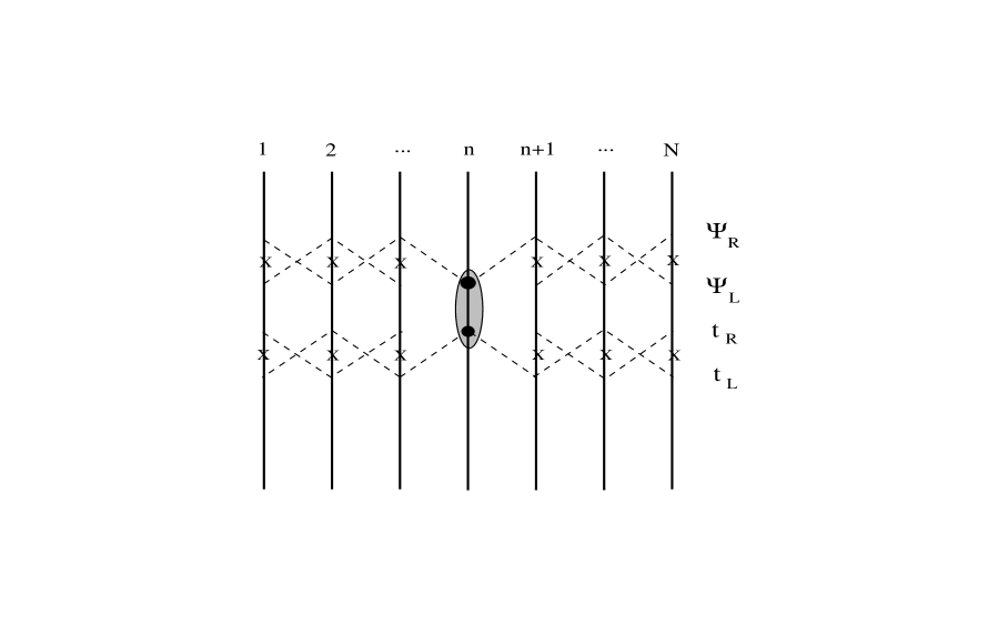
Figure 3: Pure top quark condensation by Topcolor is obtained in the limit of critical coupling on brane $n$ and decoupling to the nearest neighbors. Decoupling corresponds to taking the compactification mass scale large; the links are then denoted by dashed lines.

Figure 4: Top Seesaw Model arises when the effects of nearest neighbor vector-like fermions are retained, i.e., when these heavier states are only partially decoupled. Keeping more links maintains the seesaw. Usually we denote $t_{Rn}\sim\chi_{R}$, $t_{Ln+1}\sim\chi_{L}$, $t_{Rn+1}\sim t_{R}$ [9].

In Fig. 4, we consider the case that some of the links to nearest neighbors are not completely decoupled. Again, this can arise from renormalizations due to background fields, or due to warping [5]. Thus the mixing with heavy vector-like fermions occurs in addition to the chiral dynamics on the brane $n$. In this limit, we naturally obtain an effective Top Quark Seesaw Model [9].

In the present paper we will undertake a complete and systematic analysis of the effective 4-dimensional Top Seesaw vacuum structure and the precision electroweak constraints. This also extends the earlier works in Refs. [9, 17, 18] which studied the precision bounds on the seesaw scheme. The Higgs boson in this scheme is composite and heavy, with a mass $\sim\!1$ TeV, and the theory would seemingly be ruled out by the precision constraints on the oblique parameters $S$-$T$ [19]. We have, however, necessary compensating positive $T$ contributions coming from the additional seesaw quarks (${\chi}$), and the size of these effects can be well predicted by systematically solving the gap equations. Remarkably, a heavy Higgs boson is derived and naturally consistent with precision constraints in the Top Seesaw model.

In the recent classification of various models by Peskin and Wells [20], such compensating effects have been characterized as “conspiratorial”. Certainly many models introduce such compensating effects in an ad hoc way to achieve the consistency with the precision data. However, when the Top Seesaw was first proposed in 1998, it lay outside of the $S$-$T$ ellipse by several standard deviations [9], and the model was thus DOA (dead on arrival). Remarkably, in 1999, with a refined initial state radiation and $W$-mass determination at LEP-II, the $S$-$T$ error ellipse shifted along its major axis toward the upper right. Since then the theory remains fully consistent at the $2\sigma$ level, as illustrated in Fig. 5. Indeed the theory lies within the $S$-$T$ plot for natural values of its parameters. One might say that, with the theoretically expected scale for the seesaw partner mass of $M_{\chi}\sim 4$ TeV, the shift in the error ellipse was predicted by the theory — the Top Seesaw has therefore scored its first predictive phenomenological success! Or, more conservatively, we may view the measured error ellipse as a determination of the heavy seesaw partner mass, and obtain roughly $M_{\chi}\sim 4$ TeV. In this picture, the high precision electroweak measurements are therefore probing the mass of a heavy new particle, the $\chi$ quark, significantly above the electroweak mass scale.

Figure 5: The $68\%$ and $95\%$ C.L. $S$-$T$ contours (solid), superimposing the Standard Model curve for Higgs mass varying from $100$ GeV up to $1000$ GeV. The pre-1999 $95\%$ ellipse is shown with a dashed line. For the Top Seesaw model with a $1$ TeV composite Higgs, we show the $S$-$T$ contributions as a function of $\chi$ mass. The data is therefore consistent with a $\sim\!1$ TeV Higgs and $M_{\chi}\sim 4.0$ TeV. (The $S$-$T$ ellipses are taken from 1999 precision fit [26].)

Let us briefly summarize the logical path that leads to the Top Quark Seesaw model, irrespective of the recent interest in bosonic extra dimensions as a rationale for this scheme. Indeed, the observed large top quark mass at Tevatron is suggestive of new dynamics responsible for generating the EWSB involving intimately the top quark. The “Top quark condensation” or “Top-mode Standard Model” [13, 14, 15, 16], is the earliest and simplest idea that involves a BCS-like pairing $\left\langle\bar{t}t\right\rangle$. It predicts a top quark mass in the SM determined by the quasi-infrared fixed point [21], $m_{t}\sim 220$ GeV, provided the new dynamics scale $\Lambda$ for the condensate generation is chosen to be very large. The model involves fine-tuning in the gap equation under the large $\Lambda$ limit, and the degree of fine-tuning is of ${\cal O}(m_{t}^{2}/\Lambda^{2})$. The minimal top condensate model predicts a too heavy top quark mass, so the simplest scheme is ruled out.

In top condensation, with the fermion-bubble approximation [omitting the full renormalization group (RG) improvement inherent in [21]], it is conceptually easy to see that a dynamical mass gap $m_{\rm dyn}$ is generated and related to the weak scale through the Pagels-Stokar formula [22],

$$f_{\pi}^{2}=v_{\rm weak}^{2}=\frac{N_{c}}{16\pi^{2}}m_{\rm dyn}^{2}\ln(\Lambda^{2}/m_{\rm dyn}^{2})\,,$$ (2)

where $v_{\rm weak}=[2\sqrt{2}G_{F}]^{-1/2}\simeq 174$ GeV. This relation leads to $m_{\rm dyn}\sim 700$ GeV for a typical Topcolor breaking scale $\Lambda\sim 3.5$ TeV. Thus, the degree of fine-tuning is roughly reduced to the order of $\sim\!\left(m_{\rm dyn}/\Lambda\right)^{2}\!\sim\!(1/4)^{2}\!\sim\!10\%$, which is at a reasonable level and is actually “realistic” for the Nambu-Jona-Lasinio (NJL) model as an approximation to the full dynamics. [E.g., the NJL model with fermion loops slightly exaggerates the degree of fine-tuning, and when it fits to QCD, one has a degree of fine-tuning, roughly about $\left({\rm mass\,gap}/\Lambda\right)^{2}\!\sim\!\left(\frac{1}{3}M_{p}/M_{p}\right)^{2}\sim 11\%$, where $M_{p}\sim 1$ GeV is the mass of proton and $M_{p}/3$ the dynamical mass of constituent quarks.] If the top quark mass had been $\sim 700$ GeV, our problem would have been solved, and the EWSB would necessarily be identified with a $\bar{t}t$ condensate. Raising the scale of $\Lambda$ leads to the aforementioned fine-tuning problem and the top quark is too light to produce the full electroweak condensate.

Topcolor [7, 8] is gauge dynamics that can produce a nonzero $\left\langle\bar{t}t\right\rangle$ condensation. It involves an imbedding of QCD into a larger group, which is essentially dictated by the quantum numbers of the top quark to be $SU(3)\rightarrow SU(3)_{1}\times SU(3)_{2}\times\cdots$ (and possibly also the $U(1)_{Y}\rightarrow U(1)_{Y1}\times U(1)_{Y2}\times\cdots$). While this construction always seemed ad hoc, with latticized bosonic extra-dimensions as an organizing principle, we have seen that it becomes natural [1, 2, 5]. Topcolor can directly produce the $\left\langle\bar{t}t\right\rangle$ condensate, and the Pagels-Stokar relation (2) requires $\Lambda\sim 10^{14}$ GeV. Thus the fine-tuning $\sim\!m_{t}^{2}/\Lambda^{2}\!\sim\!10^{-23}$ becomes a severe problem in the simplest realization. Alternatively, Topcolor can produce a light top mass at the natural scale $\Lambda\sim{\cal O}(1)$ TeV, and then another strong dynamics, e.g., Technicolor, is required to provide the majority strength of the EWSB. This is known as Topcolor Assisted Technicolor (TC2) [7], and it frees one from the requirement that the top quark condensate generates all of the observed $v_{\rm weak}$. It also largely solves the problematic constraints on the Extended Technicolor (ETC), which prohibits the generation of a large mass $m_{t}\sim v_{\rm weak}$. Many interesting phenomenological consequences of this TC2 scheme arise [8, 25].

We can, alternatively, construct a Top Quark Seesaw model in which the dynamical mass term involving the top quark is of order $700$ GeV and thus is associated with the full electroweak symmetry breaking. This involves typically a pairing of the $t_{L}$ ($I=\frac{1}{2}$) with a new quark, $\chi_{R}$ ($I=0$), which has the same quantum numbers as $t_{R}$. We choose, for naturalness sake, $\Lambda\sim{\cal O}({\rm TeV})$, and hence this mass term is of the order $\sim\!700$ GeV by the Pagels-Stokar formula (2). We then incorporate an $I=0$ quark with the same quantum numbers as $t_{R}$, $\chi_{L}$, with additional mass terms, and we construct a seesaw mechanism. With the seesaw it is possible to adjust the physical mass of the top quark to its experimental value of $174$ GeV [9]. Hence, the Topcolor Seesaw mechanism can be readily implemented by introducing a pair of iso-singlet, vector-like quarks $\chi_{L}$ and $\chi_{R}$, of hypercharge $Y=4/3$, in analogy with the $t_{R}$. This model produces a bound-state Higgs boson, primarily composed of $\bar{t}_{L}\chi_{R}$ with a mass of order $\sim 1$ TeV or so, while the $\chi$ mass is at the TeV scale.

Note that the Top Seesaw model does not invoke Technicolor, but rather replaces Technicolor entirely with Topcolor. In a sense, it is a pure ETC model, where ETC (Topcolor) is sufficiently strong to form condensates. It thus offers new model building possibilities, and may allow interesting extensions to solve the flavor problem. The basic dynamics of the model can be extended to all families if one is willing to tolerate more fine-tuning. Again, extra-dimensions point the way to a full flavor model extension [5]. While there are the additional “$\chi$” quarks involved in the strong dynamics, these do not carry weak-isospin quantum numbers. This is an advantage from the viewpoint of model building, since the constraint of the $S$ parameter is essentially irrelevant for the Top Seesaw, since we have only a chiral top quark condensate in the EWSB channel, and we extend by including only vector-like fermions.

The Top Seesaw model makes a robust prediction about the nature of the electroweak condensate: the left-handed top quark is unambiguously identified as the electroweak-gauged condensate fermion. The scheme demands the presence of Topcolor interactions, but beyond the $I=1/2$ component of the EWSB, the remainder of the structure, e.g., the $\chi$ quarks and the additional strong forces which they feel, appear to be fairly arbitrary. However, as we have seen above, a remarkable aspect of the Top Seesaw model, is that the ingredients, which otherwise appear to be rather arbitrary, i.e., Topcolor, (tilting $U(1)$’s), vector-like $\chi$ quarks, etc., are all naturally given by theories of extra-dimensions where top and gauge fields propagate in the bulk [1, 2, 5]. The theory may be depicted graphically from the latticized bulk in Fig. 4 as explained above. One obtains an effective $1+3$ dimensional Lagrangian description in which all of the SM gauge groups are replicated for each Kaluza-Klein (KK) mode, e.g., for QCD we find $SU(3)\rightarrow SU(3)\times SU(3)\times\cdots$, with $N$ additional copies for $N$ KK modes. Moreover, the vector-like $\chi$ quarks can arise as the KK modes of fermions in the bulk.

As mentioned at the outset, the Top Seesaw scheme implies that, in the absence of the seesaw mechanism, the top quark would have a much larger mass, of order $\sim\!700$ GeV. This has the effect of raising the masses of all the colorons and any additional heavy gauge bosons, permitting the full Topcolor structure to be moved to somewhat higher mass scales. This gives more model-building elbow room, and may reflect the reality of new strong dynamics. We believe that the Top Seesaw is a sufficiently significant and novel, but relatively new idea in dynamical models of EWSB and opens up a large range of new model building possibilities.

In this work, we perform a systematic analysis of the dynamical vacuum structure for minimal top seesaw models by quantitatively solving the gap equations. The top mass and the full EWSB are generated together. The inclusion of bottom seesaw is further studied. We carry out the analysis using an improved broken phase formulation, in comparison to the traditional gauge-invariant formalism; the former allows us to treat all the seesaw mixing effects in a precise way and thus reliably analyze the model parameter space. The composite Higgs mass spectrum is computed by several independent approaches. We further study the precision bounds via the $S$-$T$ oblique corrections and the ${Zb\bar{b}}$ vertex correction, from which we derive nontrivial constraints on the parameter space and the composite Higgs spectrum. The effects of Topcolor instantons [7] are also analyzed, as a source to generate part or all of the bottom quark mass.

2 Dynamical Top Seesaw Model and the Gap Equations

2.1 The Minimal Model

In the minimal Top Seesaw scheme [9] the full EWSB occurs via the condensation of the left-handed top quark $t_{L}$ with a new, right-handed weak-singlet quark $\chi_{R}$. The $\chi_{R}$ quark has hypercharge $Y=4/3$ and is thus indistinguishable from the $t_{R}$. The dynamics which leads to this condensate is Topcolor, as discussed below, and no tilting $U(1)$’s are required. The fermionic mass scale of this weak-isospin $I=1/2$ condensate is $\sim 700$ GeV. This corresponds to the formation of a dynamical boundstate weak-doublet Higgs field, $H\sim(\overline{\chi_{R}}t_{L},\overline{\chi_{R}}b_{L})^{T}$. To leading order in $1/N_{c}$ this yields, via the Pagels-Stokar formula, the proper Higgs vacuum expectation value $v_{weak}=174$ GeV and the top quark $I=\frac{1}{2}$ dynamical mass term,

$$m_{t\chi}\overline{t_{L}}\,\chi_{R}\,+\,{\rm h.c.}\,,\qquad\qquad(m_{t\chi}\sim 700\,{\rm GeV})\,.$$ (3)

Moreover, the model incorporates a left-handed weak-isosinglet $\chi$ quark, with $(I,\,Y)=(0,\,4/3)$. Thus, $\chi$ quarks have an allowed Dirac mass term,

$$\mu_{\chi\chi}\overline{\chi_{L}}\chi_{R}\,+\,{\rm h.c.}\,.$$ (4)

This may be viewed as a dynamical mass through additional new dynamics (yet unspecified) at a still higher mass scale. However, since the $\chi_{R}$ and $\chi_{L}$ quarks carry the same $(I,\,Y)$ charges, we prefer to introduce Eq. (4) by hand and ignore, temporarily, its dynamical origin. Furthermore, the left-handed $\chi$ quark can form an allowed weak-singlet Dirac mass term with the right-handed top quark, leading to,

$$\mu_{\chi t}\overline{\chi_{L}}\,t_{R}\,+\,{\rm h.c.}\,,$$ (5)

which again may be viewed as a dynamical mass term in an enlarged theory. There is no direct left-handed top condensate with the right-handed anti-top in this scheme, since they do not share the same strong Topcolor dynamics (cf. Sec. 2.2). Thus, the resulting mass matrix for the $t-\chi$ system is,

$$-\left(\overline{t_{L}}~{}~{}\overline{\chi_{L}}\right)\left\lgroup\begin{array}[]{cc}0&m_{t\chi}\\[5.69046pt] \mu_{\chi t}&\mu_{\chi\chi}\\ \end{array}\right\rgroup\left(\!\!\begin{array}[]{c}t_{R}\\ \chi_{R}\end{array}\!\!\right)\,+\,{\rm h.c.}\,.$$ (10)

This seesaw mass matrix can be exactly diagonalized by rotating the left- and right-handed fields,

$$\left(\begin{array}[]{c}t_{L}\\[5.69054pt] \chi_{L}\end{array}\right)={\mathbf{K}^{t}_{L}}\left(\begin{array}[]{c}t^{\prime}_{L}\\[5.69054pt] \chi^{\prime}_{L}\end{array}\right),~{}~{}~{} ~{}~{}~{}\left(\begin{array}[]{c}t_{R}\\[5.69054pt] \chi_{R}\end{array}\right)={\mathbf{K}^{t}_{R}}\left(\begin{array}[]{c}t^{\prime}_{R}\\[5.69054pt] \chi^{\prime}_{R}\end{array}\right),$$ (19)

with

$${\mathbf{K}^{t}_{L}}=\left\lgroup\begin{array}[]{rr}\!\!c_{L}&s_{L}\\ \!\!-s_{L}&c_{L}\end{array}\right\rgroup,~{}~{}~{} ~{}~{}~{}{\mathbf{K}^{t}_{R}}=\left\lgroup\begin{array}[]{rr}\!\!-c_{R}&s_{R}\\ \!\!s_{R}&c_{R}\end{array}\right\rgroup,$$ (24)

which are determined by obtaining the (positive) mass eigenvalues, $m_{t}$ and $M_{\chi}$. For convenience, we have used the abbreviation $s_{L}=\sin\theta_{L}$, and so forth. Our parametrization has also implicitly assumed the mass matrix to be real, and thus orthogonal. In the absence of further ingredients, this will always be the case because any stray complex phase in the mass matrix can be absorbed by redefining the fermion fields. The (rotated) mass eigenstate fields are denoted by $t^{\prime}$ and $\chi^{\prime}$ to distinguish them from the interaction eigenstate fields $t$ and $\chi$ . The mass eigenvalues and rotation angles are given by,

$$m^{2}_{t} = \frac{1}{2}\left[\,\mu^{2}_{\chi\chi}+\mu^{2}_{\chi t}+m^{2}_{t\chi}-\sqrt{\left(\mu^{2}_{\chi\chi}+\mu^{2}_{\chi t}+m^{2}_{t\chi}\right)^{2}-4\,\mu^{2}_{\chi t}\,m^{2}_{t\chi}}\,\right]\,,$$

$$\longrightarrow \left.\frac{m_{t\chi}^{2}\mu_{\chi t}^{2}}{\mu_{\chi t}^{2}+\mu_{\chi\chi}^{2}}\right|_{(\mu_{\chi\chi}\gg\mu_{\chi t},\,m_{t\chi})},$$

$$m^{2}_{\chi} = \frac{1}{2}\left[\,\mu^{2}_{\chi\chi}+\mu^{2}_{\chi t}+m^{2}_{t\chi}+\sqrt{\left(\mu^{2}_{\chi\chi}+\mu^{2}_{\chi t}+m^{2}_{t\chi}\right)^{2}-4\,\mu^{2}_{\chi t}\,m^{2}_{t\chi}}\,\right]\,,$$

$$\longrightarrow \left.\mu_{\chi\chi}^{2}+\mu^{2}_{\chi t}\right|_{(\mu_{\chi\chi}\gg\mu_{\chi t},\,m_{t\chi})},$$

$$\left(\!\!\begin{array}[]{c}s_{L}\\ c_{L}\end{array}\!\!\right) = \frac{1}{\sqrt{2}}\left[1\mp\frac{\mu^{2}_{\chi\chi}+\mu^{2}_{\chi t}-m^{2}_{t\chi}}{M^{2}_{\chi}-m^{2}_{t}}\right]^{\frac{1}{2}}\,,$$ (29)

$$\left(\!\!\begin{array}[]{c}s_{R}\\ c_{R}\end{array}\!\!\right) = \frac{1}{\sqrt{2}}\left[1\mp\frac{\mu^{2}_{\chi\chi}-\mu^{2}_{\chi t}+m^{2}_{t\chi}}{M^{2}_{\chi}-m^{2}_{t}}\right]^{\frac{1}{2}}\,.$$ (32)

The fermionic mass matrix thus admits a conventional seesaw mechanism, yielding the physical top quark mass as an eigenvalue that is $\sim m_{t\chi}\mu_{\chi t}/\mu_{\chi\chi}\ll m_{t\chi}\sim 700$ GeV. The top quark mass can be adjusted to its experimental value by the choice of $\mu_{\chi t}/\mu_{\chi\chi}$. The diagonalization of the fermionic mass matrix does not affect the physical vacuum expectation value (VEV), $v_{weak}\simeq 174$ GeV, of the composite Higgs doublet. Indeed, the Pagels-Stokar formula is now modified as,

$$v_{\rm weak}^{2}\equiv f_{\pi}^{2}\simeq\frac{N_{c}}{16\pi^{2}}\frac{m_{t}^{2}}{\sin^{2}\theta_{R}}\left(\ln\frac{\Lambda^{2}}{\overline{M}^{2}}+c\right)$$ (33)

where $m_{t}$ is the physical top mass, $\sin\theta_{R}=s_{R}\approx\mu_{\chi t}/\mu_{\chi\chi}$ the right-handed seesaw angle, $\overline{M}=\sqrt{\mu_{{\chi}t}^{2}+\mu_{{\chi}{\chi}}^{2}}$, and $c$ denotes sub-leading terms, and we expect $c\sim{\cal{O}}(1)$.

The Pagels-Stokar formula now differs from that obtained (in large-$N_{c}$ approximation) for pure top quark condensation models, by a large enhancement factor $1/\sin^{2}\theta_{R}$.  This is a direct consequence of the seesaw mechanism. The mechanism incorporates $\psi_{L}=(t_{L},\,b_{L})$, which provides the source of the weak-isospin $I=1/2$ quantum number of the composite Higgs boson, and thus the origin of the EWSB vacuum condensate. Note that we have separated the problem of EWSB from the weak-isosinglet physics in the $\chi_{L,R}$ and $t_{R}$ sector, which is an advantage of the seesaw mechanism since the electroweak constraints are not so restrictive on the isosinglets.

2.2 Topcolor Dynamics

Let us turn to some of the dynamical questions, e.g., how does Topcolor produce the dynamical $m_{t\chi}$ mass term? We proceed by introducing an embedding of QCD into the gauge groups $SU(3)_{1}\otimes SU(3)_{2}$, with coupling constants $h_{1}$ and $h_{2}$, respectively. These symmetry groups are broken down to $SU(3)_{QCD}$ at a high mass scale. We assign the representations for relevant fermions under the full set of gauge groups $SU(3)_{1}\otimes SU(3)_{2}\otimes SU(2)_{W}\otimes U(1)_{Y}$ as below,

$$\psi_{L}\!:~{}~{}({\bf 3,1,2,}\,+1/3)\,,~{}~{}~{}~{}~{}\chi_{R}\!:~{}~{}({\bf 3,1,1,}\,+4/3)\,,~{}~{}~{}~{}~{}t_{R},\,\chi_{L}\!:~{}~{}({\bf 1,3,1,}\,+4/3)\,.$$ (34)

This set of fermions is incomplete; the representation specified has $[SU(3)_{1}]^{3}$, $[SU(3)_{2}]^{3}$, and $U(1)_{Y}[SU(3)_{1,2}]^{2}$ gauge anomalies. These anomalies will be canceled by fermions associated with either the dynamical breaking of $SU(3)_{1}\otimes SU(3)_{2}$, or with the $b$ quark mass generation (an explicit realization of the latter case will be given in Sec. 3). The crucial dynamics of the EWSB and top quark mass generation will not depend on the details of these additional fermions. Schematically, the picture looks like:

$\ \ \ \ \ \ \ \ ~{}~{}SU(3)_{1}$          $\ \ \ \ \ \ \,\,SU(3)_{2}$          

$\left\lgroup\begin{array}[]{c}\,\left(\begin{array}[]{c}t_{L}\\ b_{L}\end{array}\right)\\[11.38109pt] \chi_{R}\\[5.69054pt] \cdots\end{array}\right\rgroup$       $~{}\left\lgroup\begin{array}[]{c}\left(\begin{array}[]{c}t_{R}\\ b_{R}\end{array}\right)\\[11.38109pt] \chi_{L}\\[5.69054pt] \cdots\end{array}\right\rgroup$

This can be viewed as a two lattice-brane approximation to a higher dimensional model with localized chiral fermions [5].

We further introduce a scalar field, ${{\mathbf{\Phi}}}$, transforming as $({\bf\overline{3},3,1,}\,0)$, with a negative mass $M_{{\mathbf{\Phi}}}^{2}$ and an associated quartic potential such that ${\mathbf{\Phi}}$ develops a diagonal VEV,

$$\langle{{\mathbf{\Phi}}}^{i}_{j}\rangle=V\;\delta_{j}^{i}\,,$$ (35)

and Topcolor group is broken down to the usual QCD,

$$SU(3)_{1}\otimes SU(3)_{2}\longrightarrow SU(3)_{QCD}\,,$$ (36)

yielding massless gluons and an octet of degenerate colorons with mass $\Lambda$ given by

$$\Lambda^{2}=(h_{1}^{2}+h_{2}^{2})\,{V}^{2}\,.$$ (37)

${\mathbf{\Phi}}$ is just the Wilson link connecting the two branes in the $4+1$ picture, and $V$ the inverse compactification scale. Alternatively, from a pure $3+1$ perspective this symmetry breaking can arise dynamically, which is akin to dimensional deconstruction [4]. We will describe ${\mathbf{\Phi}}$ as a fundamental field in the present model for the sake of simplicity.

The scalar ${\mathbf{\Phi}}$ also has the correct quantum numbers to form a Yukawa interaction with the singlet seesaw quarks $\chi_{L,R}$ and thus provides the requisite mass term $\mu_{\chi\chi}$,

$$-y_{\chi}\,\overline{\chi_{R}}\,{\mathbf{\Phi}}\,\chi_{L}+{\rm h.c.}\longrightarrow-\mu_{\chi\chi}\,\overline{\chi}\chi\,.$$ (38)

This also happens automatically in the latticized extra-dimension scheme where this term plays the role of the fermion (hopping) kinetic term. We stress that this is an electroweak singlet mass term. In this scheme $y_{\chi}$ is a perturbative coupling constant so that ${V}\gg\mu_{\chi\chi}$. Finally, as both $t_{R}$ and $\chi_{L}$ carry identical Topcolor and $U(1)_{Y}$ quantum numbers, we should also include the explicit weak-singlet mass term, of the form, $\mu_{\chi t}\overline{\chi_{L}}\,t_{R}+{\rm h.c.}$ .

At energy scales below the coloron mass, the effective Lagrangian of this minimal model is $SU(3)_{C}\otimes SU(2)_{W}\otimes U(1)$ invariant and can be written as,

$${\cal{L}}_{0}={\cal{L}}_{\rm kinetic}-(\mu_{\chi\chi}\,\overline{\chi_{L}}\,\chi_{R}+\mu_{\chi t}\,\overline{\chi_{L}}\,t_{R}+{\rm h.c.})+{\cal{L}}_{\rm int}\,.$$ (39)

${\cal{L}}_{\rm int}$ contains the residual Topcolor interactions from the exchange of the massive colorons, and can be written as an operator product expansion,

$${\cal{L}}_{\rm int}=-\frac{h^{2}_{1}}{\Lambda^{2}}\left(\overline{\psi_{L}}\,\gamma^{\mu}\frac{T^{a}}{2}\psi_{L}\right)\left(\overline{\chi_{R}}\,\gamma_{\mu}\frac{T^{a}}{2}\chi_{R}\right)+LL+RR+\cdots\,,$$ (40)

where $LL$ $(RR)$ refers to left-handed (right-handed) current-current interactions and $T^{a}$’s are the broken $SU(3)$ generators. Since the Topcolor interactions are strongly coupled, forming boundstates, higher dimensional operators might have a significant effect on the low energy theory. However, if the full Topcolor dynamics induces chiral symmetry breaking through a second order (or weakly first order) phase transition, then one can analyze the theory using the fundamental degrees of freedom, namely the quarks, at scales significantly lower than the Topcolor scale. We will assume that this is the case, which implies that the effects of the higher dimensional operators are suppressed by powers of the Topcolor scale, and it is sufficient to keep in the low energy theory only the effects of the operators shown in Eq. (40). Furthermore, the $LL$ and $(RR)$ interactions do not affect the low-energy effective potential in the large-$N_{c}$ limit, so we will ignore them. (One should keep in mind that these interactions may have other effects, such as contributions to the custodial symmetry violation parameter $T$, but these effects are negligible if the Topcolor scale is in the multi-TeV range).

To leading order in $1/N_{c}$ and upon performing the familiar Fierz rearrangement, we obtain the following scalar-type NJL [23] interaction,

$${\cal{L}}_{\rm int}=\frac{h_{1}^{2}}{\Lambda^{2}}(\overline{\psi_{L}}\,\chi_{R})\,(\overline{\chi_{R}}\,\psi_{L})~{}.$$ (41)

It is convenient to pass to a partial mass eigenbasis with the following transformations for right-handed fields,

$$\chi_{R}\rightarrow\cos\theta\;\chi_{R}-\sin\theta\;t_{R}\,,~{}~{}~{}~{}~{}\quad t_{R}\rightarrow\cos\theta\;t_{R}+\sin\theta\;\chi_{R}\,,$$ (42)

where

$$\tan\theta=\frac{\mu_{\chi t}}{\mu_{\chi\chi}}\,.$$ (43)

In this basis, the NJL Lagrangian takes the form,

$${\cal{L}}_{0} = {\cal{L}}_{\rm kinetic}-\overline{M}\,\overline{\chi_{R}}\,\chi_{L}+{\rm h.c.}$$ (44)

$$+\frac{h_{1}^{2}}{\Lambda^{2}}\left[\overline{\psi_{L}}\,\left(\cos\theta\;\chi_{R}-\sin\theta\;t_{R}\right)\right]\left[\left(\cos\theta\;\overline{\chi_{R}}-\sin\theta\;\overline{t_{R}}\right)\,\psi_{L}\right]\,,$$

with

$$\overline{M}=\sqrt{\mu_{\chi\chi}^{2}+\mu_{\chi t}^{2}}~{}.$$ (45)

2.3 Gap Equation Analysis

At this stage we have the choice of using the renormalization group (RG), or to study the mass gap equation for $m_{t\chi}$. Ultimately these should be equivalent. The RG approach requires the construction of the effective potential of the composite Higgs boson, and its minimization. The gap equations get us there directly. A further rationale for studying the gap equations is that they in principle allow one to explore the limits, such as $\overline{M}>\Lambda$ which are conceptually more difficult with the renormalization group. (The dimension-6 operator makes no sense above the scale $\Lambda$ in the RG, but the cut-off theory can still be expressed in the gap equation language.) In the following, we will start with the gap equation analysis, and we find it instructive to begin by treating $m_{t\chi}$ as a mass-insertion and examine its dependence on the parameters $\overline{M}$ and $\theta$. An improved derivation of the seesaw gap equation without mass-insertion will be given in Appendix-A1 and Sec. 2.4.

To derive gap equations, we expand the NJL vertex in Eq. (44) and find that the four individual vertices, $\left(\overline{t_{L}}{\chi}_{R}\right)\left(\overline{{\chi}_{R}}t_{L}\right)$,  $\left(\overline{t_{L}}t_{R}\right)\left(\overline{t_{R}}t_{L}\right)$,  $\left(\overline{t_{L}}t_{R}\right)\left(\overline{{\chi}_{R}}t_{L}\right)$,  and $\left(\overline{t_{R}}t_{L}\right)\left(\overline{t_{L}}{\chi}_{R}\right)$,  can form two types of dynamical condensates, $\langle\overline{t_{L}}{\chi}_{R}\rangle$ and $\langle\overline{t_{L}}t_{R}\rangle$. Correspondingly, we have two mass-gap terms,

$$-\,m_{t\chi}\overline{t}_{L}\chi_{R}\,-\,m_{tt}\overline{t}_{L}t_{R}\,,$$ (46)

where the diagonal mass $m_{tt}$ can be conveniently put into the top propagator while the off-diagonal mass $m_{t\chi}$ will be included up to ${\cal O}(m_{t\chi}^{3})$ in the present analysis. We can then write down the two gap equations for $m_{t\chi}$ and $m_{tt}$, as graphically shown in Fig. 6. It is clear that these are the large-$N_{c}$ Schwinger-Dyson equations [expanded up to ${\cal O}(m_{t\chi}^{3})$] for the NJL-Lagrangian (44). From Fig. 6, we derive,

$$\begin{array}[]{c}m_{t\chi}=\displaystyle-sc\frac{h_{1}^{2}}{\Lambda^{2}}\sum_{j=1}^{4}\Delta_{j}\,,~{}~{}~{}~{}~{}m_{tt}=\displaystyle-s^{2}\frac{h_{1}^{2}}{\Lambda^{2}}\sum_{j=1}^{4}\Delta_{j}\,,\\[22.76219pt] \longrightarrow\displaystyle\frac{m_{t\chi}}{m_{tt}}=\frac{s}{c}=\frac{\mu_{\chi t}}{\mu_{\chi\chi}}\,,\end{array}$$ (47)

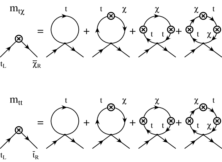
Figure 6: Top seesaw gap equations for $m_{t\chi}$ and $m_{tt}$.

where $(s,\,c)=(\sin\theta,\,\cos\theta)$ and the term $\sum_{j=1}^{4}\Delta_{j}$ represents the sum of four loop-integrals on the right-hand side of each gap equation in Fig. 6. It is important to note that the same loop graphs appear in both gap equations for $m_{t\chi}$ and $m_{tt}$ so that we have the relation $m_{tt}/m_{t\chi}=s/c$ as above. This means that the two coupled gap equations are actually reduced to one independent gap equation, say, for $m_{t\chi}$. By explicit calculation of the loop integrals, we write this gap equation in the following form, up to ${\cal O}(m_{t\chi}^{3})$,

$$\begin{array}[]{l}m_{t\chi}\,=\,m_{t\chi}\displaystyle\frac{\kappa}{\kappa_{c}}\left[1-\frac{m_{t\chi}^{2}}{\Lambda^{2}}\left((1+s^{2})\ln\left(\frac{\Lambda^{2}}{\overline{M}^{2}}+1\right)-\frac{c^{2}\Lambda^{2}}{\Lambda^{2}+{\overline{M}}^{2}}+\frac{s^{4}}{c^{2}}\ln\left(\frac{c^{2}}{s^{2}}\frac{\Lambda^{2}}{m_{t\chi}^{2}}+1\right)\right)\right.\\[17.07164pt] \left.\displaystyle\hskip 85.35826pt\,-\,c^{2}\frac{{\overline{M}}^{2}}{\Lambda^{2}}\ln\left(\frac{\Lambda^{2}}{{\overline{M}}^{2}}+1\right)\right]+{\cal O}(m_{t\chi}^{4})\,,\end{array}$$ (48)

where for convenience we have used the definitions, $\kappa=h_{1}^{2}/(4\pi)$ and $\kappa_{c}=2\pi/N_{c}$. There are several ways to see that these reproduce normal top condensation in the decoupling limit. For instance, taking $\overline{M}\rightarrow\infty$ for fixed $\Lambda$ and using the relation $m_{t\chi}=m_{tt}(s/c)$, we find,

$$m_{tt}\,=\,m_{tt}\displaystyle\frac{\kappa}{\kappa_{c}}\left[1-\frac{m_{tt}^{2}}{\Lambda^{2}}\ln\left(\frac{\Lambda^{2}}{m_{tt}^{2}}+1\right)\right]\,,$$ (49)

which is just the familiar top condensation gap equation, with $m_{tt}$ the dynamical top quark mass. Here we have decoupled $\chi_{L}$ and $\chi_{R}$ with $\overline{M}\rightarrow\infty$. We can also obtain top condensation by setting $\sin^{2}\theta=s^{2}=0$ and $\overline{M}\rightarrow 0$, which decouples $\chi_{L}$ and $t_{R}$, and causes $\chi_{R}$ to play the role of $t_{R}$. A main advantage of this mass-insertion gap equation (48) is that it allows us to analytically solve for $m_{t\chi}$ (ignoring a small ${\cal O}(s^{4})$ term),

$$m_{t\chi}~{}\simeq~{}\displaystyle\Lambda\left[\frac{\displaystyle 1-\frac{\kappa_{c}}{\kappa}-c^{2}\frac{{\overline{M}}^{2}}{\Lambda^{2}}\ln\left(\frac{\Lambda^{2}}{{\overline{M}}^{2}}+1\right)}{\displaystyle(1+s^{2})\ln\left(\frac{\Lambda^{2}}{{\overline{M}}^{2}}+1\right)-\frac{c^{2}\Lambda^{2}}{\Lambda^{2}+{\overline{M}}^{2}}}\right]^{\frac{1}{2}},$$ (50)

where we have discarded the trivial solution $m_{t\chi}=0$.

This clearly shows that for the fixed $\kappa/\kappa_{c}>1$, the condensate turns off like a second order phase transition as we raise the scale $\overline{M}$. This is essentially to compensate the decoupling of the heavy fermion in the loop of mass $\overline{M}$. The gap equation (48) or (49) also shows that we require super-critical coupling as the mass $\overline{M}$ becomes large. We can further derive the effective seesaw critical coupling $\kappa_{c}^{\rm eff}$ from the gap equation (48) or (50) by setting $m_{t\chi}=0$, i.e., we have,

$$\frac{~{}\kappa_{c}^{\rm eff}}{\,\kappa_{c}}~{}=~{}\frac{1}{\displaystyle 1-c^{2}\frac{{\overline{M}}^{2}}{\Lambda^{2}}\ln\left(\frac{\Lambda^{2}}{{\overline{M}}^{2}}+1\right)}\,\,,$$ (51)

which is displayed in Fig. 7 as a function of ${\overline{M}}/\Lambda$. For $\kappa>\kappa_{c}^{\rm eff}$, we have $m_{t\chi}>0$. We see that $\kappa_{c}^{\rm eff}=\kappa_{c}$ for ${\overline{M}}=0$, and as ${\overline{M}}$ increases the effective seesaw critical coupling $\kappa_{c}^{\rm eff}$ moves above $\kappa_{c}(=2\pi/N_{c})$ implying that stronger Topcolor force is required compared to the non-seesaw case. Finally, we note that using the complete seesaw diagonalization (19)-(24) and the NJL-vertex (41), we can derive the exact large-$N_{c}$ seesaw gap equation without using a mass-insertion approximation (cf. Appendix-A1). This will allow us to reliably analyze the full seesaw parameter space.

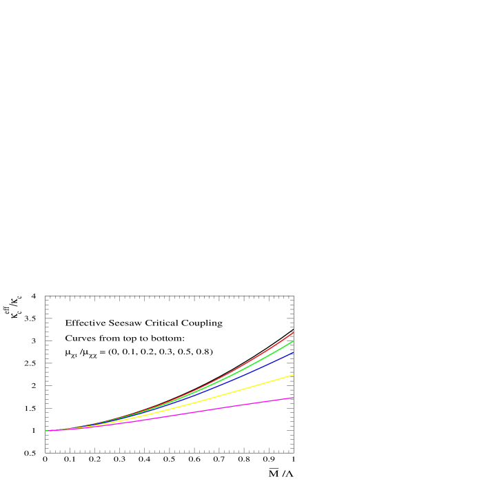
Figure 7: Effective seesaw critical coupling $\kappa_{c}^{\rm eff}$ (scaled by constant $\kappa_{c}\equiv 2\pi/3$) as a function of $\overline{M}/\Lambda$, for ${\tan\theta}=\mu_{\chi t}/\mu_{\chi\chi}=(0,\,0.1,\,0.2,\,0.3,\,0.5,\,0.8)$.

The electroweak structure of the low energy theory is best read off from the effective Lagrangian, which may be derived from the traditional gauge-invariant renormalization group analysis as below. We proceed by rewriting the NJL interaction (41) with the introduction of an auxiliary color-singlet field, $\Phi_{0}$, which becomes the unrenormalized composite Higgs doublet,

$${\cal{L}}_{0}={\cal{L}}_{\rm kinetic}-\left[\,\overline{M}\,\overline{\chi_{R}}\,\chi_{L}+h_{\rm 1}\,\overline{\psi_{L}}\,(\cos\theta\;\chi_{R}-\sin\theta\;t_{R})\,\Phi_{0}+{\rm h.c.}\right]-\Lambda^{2}\Phi_{0}^{\dagger}\Phi_{0}~{}.$$ (52)

To derive the effective Lagrangian at a low energy scale $\mu$, we integrate out the modes of momenta $M\geq|k|\geq\mu$. For $\mu<{\overline{M}}<\Lambda$, the heavy field $\chi$ decouples, so that we have,

$${\cal{L}}_{\mu<\overline{M}}={\cal{L}}_{\rm kinetic}-h_{1}\sin\theta\left(\overline{\psi_{L}}t_{R}\,\Phi_{0}+{\rm h.c.}\right)+Z_{\Phi}\left|D\Phi_{0}\right|^{2}-\widetilde{M}_{\Phi}^{2}(\mu)\Phi_{0}^{\dagger}\Phi_{0}-\widetilde{\lambda}\left(\Phi_{0}^{\dagger}\Phi_{0}\right)^{2},$$ (53)

where the effective scalar wave-function renormalization, mass term and quartic coupling are given by,

$$Z_{\Phi}(\mu) = \displaystyle\frac{1}{2}\frac{\kappa}{\kappa_{c}}\left[\ln\left(\frac{\Lambda^{2}}{\overline{M}^{2}}\right)+\sin^{2}\!\theta\,\ln\left(\frac{\overline{M}^{2}}{\mu^{2}}\right)+{\cal O}(1)\right]\,,$$

$$\widetilde{M}_{\Phi}^{2}(\mu) = \displaystyle\Lambda^{2}-\displaystyle\frac{\kappa}{\kappa_{c}}\left[\Lambda^{2}-\cos^{2}\!\theta\,{\overline{M}}^{2}\ln\left(\frac{\Lambda^{2}}{{\overline{M}}^{2}}\right)+{\cal O}({\overline{M}}^{2},\,\mu^{2})\right]\,,$$ (54)

$$\widetilde{\lambda}(\mu) = \displaystyle 2\pi\frac{\kappa^{2}}{\kappa_{c}}\left[\ln\left(\frac{\Lambda^{2}}{\overline{M}^{2}}\right)+\sin^{4}\!\theta\,\ln\left(\frac{\overline{M}^{2}}{\mu^{2}}\right)+{\cal O}(1)\right]\,,$$

where $(\kappa,\,\kappa_{c})=(h_{1}^{2}/4\pi,\,2\pi/N_{c})$ .  These relations hold for $\mu<\overline{M}$ in the large-$N_{c}$ approximation, and illustrate the decoupling of the $\chi$ field at the scale $\mu<\overline{M}$. In the limit $\sin\!\theta\ll 1$, the induced couplings are those of the usual NJL model; but the Higgs doublet is predominantly a boundstate of $\overline{\chi_{R}}\psi_{L}$, and the corresponding fermion loop, with loop-momentum ranging over ${\overline{M}}<|k|<\Lambda$, controls most of the renormalization group evolution of the effective Lagrangian.

In order for the composite Higgs doublet to develop a VEV, the Topcolor $SU(3)_{1}$ gauge force must be super-critical, as indicated by the preceeding gap equation analysis. Once $\kappa(=h_{1}^{2}/4\pi)$ is super-critical, we are free to tune the renormalized Higgs boson mass, $M_{\Phi}^{2}(\mu)=\widetilde{M}_{\Phi}^{2}(\mu)/Z_{\Phi}$, to any desired value. This implies that we are free to adjust the renormalized VEV of the Higgs doublet to the electroweak value, $\langle\Phi\rangle=v/\sqrt{2}\simeq 174$ GeV. The renormalized effective Lagrangian at $\mu<{\overline{M}}$ takes the form,

$${\cal{L}}_{\mu<\overline{M}}={\cal{L}}_{\rm kinetic}-g_{t}\sin\!\theta\left(\overline{\psi_{L}}t_{R}\,\Phi+{\rm h.c.}\right)+\left|D\Phi\right|^{2}-M_{\Phi}^{2}(\mu)\,\Phi^{\dagger}\Phi-\lambda(\Phi^{\dagger}\Phi)^{2}$$ (55)

where,

$$\Phi=\Phi_{0}\sqrt{Z_{\Phi}}\,,~{}~{}~{}~{}g_{t}=\frac{h_{\rm 1}}{\sqrt{Z_{\Phi}}}\,,~{}~{}~{}~{}M_{\Phi}^{2}(\mu)=\frac{\widetilde{M}_{\Phi}^{2}(\mu)}{Z_{\Phi}}\,,~{}~{}~{}~{}\lambda=\frac{\widetilde{\lambda}}{Z_{\Phi}^{2}}\,.$$ (56)

When the Topcolor interaction is super-critical, $\Phi$ becomes tachyonic at low energy scales, $\widetilde{M}^{2}_{\Phi}(\mu\rightarrow 0)<0$ and a dynamical condensate will be induced. This condensate breaks the electroweak symmetry ${SU(2)}_{L}\otimes{U(1)}_{Y}\rightarrow{U(1)}_{EM}$ and induces mixing between the top and $\chi$ fields. In the minimal top seesaw model the physical particle spectrum can be readily seen by writing the Higgs doublet in the unitary gauge, $\,{\Phi}=\frac{1}{\sqrt{2}}\left(v+h,0\right)^{T},\,$ where $h$ is the neutral Higgs boson of the theory. The resulting top quark mass can be read off from the renormalized Lagrangian,

$$m_{t}\,=\,\displaystyle\frac{g_{t}\,v}{\sqrt{2}}\,\sin\theta\,,$$ (57)

which corresponds to the Pagels-Stokar formula in the form of Eq. (33).

Finally, by minimizing the effective Higgs potential in Eq. (55) and using the results in Eq. (2.3), we can derive the approximate formula for the physical Higgs mass by keeping the leading logarithmic terms,

$$M_{h}\,\approx\,2m_{t\chi}\,,$$ (58)

which shows that the physical Higgs mass is about two times of the dynamical mass gap, as expected from the usual large-$N_{c}$ bubble approximation [15, 23]. In the subsection 2.6, we will derive a more precise $M_{h}$ using two improved analyses.

2.4 Tadpole Condition and Improved Analysis in the Broken Phase

Before proceeding to perform the numerical analysis for gap equations, we consider an alternative (yet equivalent) derivation of the gap equation based on the Higgs tadpole condition in the broken phase of the effective theory. (For a simpler example of a broken phase analysis in NJL, see [24]). We also present the improved RG analysis in the broken phase of the low energy theory, which allows us to precisely treat the seesaw mass diagonalization and the mixing effects in Higgs Lagrangian. [This is unlike the usual gauge-invariant RG analysis around Eq. (52) where the Higgs vacuum is unshifted and thus the exact seesaw mass diagonalization is not allowed.] As a consequence, the Higgs mass and its Yukawa coupling can be more precisely analyzed in the present broken phase formalism. We begin by choosing the unitary gauge of the Higgs doublet and shifting the bare field $\Phi_{0}$ to the broken phase vacuum,

$${\Phi}_{0} = \frac{1}{\sqrt{2}}\left(\!\begin{array}[]{c}{v}_{0}+{h}_{0}\\[8.53581pt] 0\end{array}\!\right),$$ (61)

which results in the fermionic seesaw mass matrix given in Eq. (10). Thus, the effective Lagrangian at the scale $\mu=\Lambda$ can be written as,

$$\begin{array}[]{ll}{\cal L}_{\Lambda}&\!\!\!=-\left(\overline{t_{L}}~{}~{}\overline{\chi_{L}}\right)\left\lgroup\begin{array}[]{cc}0&m_{t\chi}\\[5.69046pt] \mu_{\chi t}&\mu_{\chi\chi}\\ \end{array}\right\rgroup\left(\!\!\begin{array}[]{c}t_{R}\\ \chi_{R}\end{array}\!\!\right)-\displaystyle\frac{h_{1}}{\sqrt{2}}\overline{t_{L}}{\chi}_{R}h_{0}+{\rm h.c.}-\frac{1}{2}\Lambda^{2}h_{0}^{2}-\Lambda^{2}v_{0}h_{0}\\[14.22636pt] &\!\!\!=-m_{t}\overline{t^{\prime}}t^{\prime}-M_{\chi}\overline{{\chi}^{\prime}}{\chi}^{\prime}-\frac{1}{2}\Lambda^{2}h_{0}^{2}-\Lambda^{2}v_{0}h_{0}-\displaystyle\frac{h_{1}}{\sqrt{2}}\left[c_{L}\,\overline{t_{L}^{\prime}}+s_{L}\,\overline{\chi^{\prime}}_{L}\right]\left[s_{R}\,t_{R}^{\prime}+c_{R}\,\chi_{R}^{\prime}\right]h_{0}+{\rm h.c.}\,,\end{array}$$ (62)

where we have performed the exact seesaw diagonalization according to Eqs. (19)-(24). Now, we evolve the Lagrangian down to the scale $\mu\,(<M_{\chi}\leq\Lambda)$ by integrating out the momenta $k\in(\mu,\,\Lambda)$. The heavy quark ${\chi}$ decouples and we arrive at the renormalized broken phase Lagrangian,

$$\begin{array}[]{l}{\cal L}_{\mu<M_{\chi}}=\displaystyle-m_{t}\overline{t^{\prime}}t^{\prime}-\displaystyle\frac{~{}g_{t}}{\sqrt{2}}c_{L}s_{R}\overline{t^{\prime}}t^{\prime}h+\frac{1}{2}\left(\partial_{\mu}h\right)^{2}-\Delta\widetilde{T}h\displaystyle-\frac{1}{2}M_{h}^{2}h^{2}-V_{\rm int}\left(Z_{h}^{-1}h\right)\end{array}$$ (63)

where $\,g_{t}=h_{1}/\sqrt{Z_{h}}\,$ and  $V_{\rm int}\left(Z_{h}^{-1}h\right)$  contains the effective Higgs self-interactions. The Higgs tadpole term $\Delta\widetilde{T}$ and mass term $M_{h}^{2}$ are defined by,

$$\Delta\widetilde{T}=\left(Z_{h}^{-\frac{1}{2}}v\Lambda^{2}+\delta\widetilde{T}\right)Z_{h}^{-\frac{1}{2}}\,,~{}~{}~{}~{}M_{h}^{2}=(\Lambda^{2}+\delta\widetilde{M}^{2}_{h})/Z_{h}\,,$$ (64)

with $\delta\widetilde{T}$ and $\delta\widetilde{M}^{2}_{h}$ computed from the one-loop Higgs tadpole and self-energy corrections, respectively. The Higgs tadpole condition,  $\Delta\widetilde{T}=0$,  results in,

$$v_{0}\Lambda^{2}+\delta\widetilde{T}=0\,,$$ (65)

where $\delta\widetilde{T}$ comes from one-loop tadpole diagrams (cf. Fig. 8). Note that the tadpole loops in $\delta\widetilde{T}$ will be integrated from zero momentum to the cutoff $\Lambda$ (independent of the renormalization scale $\mu$) as they are really vacuum graphs with vanishing external momentum. The equation (65) is just the minimization condition of the Higgs potential in its broken phase, and is equivalent to the gap equation derived from the NJL formalism in Sec. 2.3 and Appendix-A1, as will be clear shortly. Fig. 8 shows that the condition in Eq. (65) actually represents the exact large-$N_{c}$ gap equation without mass-insertion. [The mass-insertion tadpole condition, fully equivalent to gap equation (48) in Sec. 2.3, will be given in Appendix-A2.] Now, using the relation $m_{t\chi}=h_{1}v_{0}/\sqrt{2}$, we can explicitly derive, from Eq. (65), a single gap equation for $m_{t\chi}$,

$$\vspace*{3.5mm}m_{t\chi}~{}=~{}\frac{\kappa}{\kappa_{c}}\left\{c_{L}s_{R}\left(m_{t}-\frac{m_{t}^{3}}{\Lambda^{2}}\ln\left[\frac{\Lambda^{2}+m_{t}^{2}}{m_{t}^{2}}\right]\right)+s_{L}c_{R}\left(m_{\chi}-\frac{m^{3}_{\chi}}{\Lambda^{2}}\ln\left[\frac{\Lambda^{2}+m_{\chi}^{2}}{m_{\chi}^{2}}\right]\right)\right\}\,,$$ (66)

where $(\kappa,\,\kappa_{c})=(h_{1}^{2}/4\pi,\,2\pi/N_{c})$. Eq. (66) is the same as the exact large-$N_{c}$ NJL gap equation derived in Appendix-A1. It also reduces back to the approximate mass-insertion gap equation (48) (cf. Sec. 2.3 and Appendix-A2) after expanding the seesaw rotation angles and mass eigenvalues up to ${\cal O}(m_{t\chi}^{3})$, as we have verified. This provides a consistency check of our analysis. Since the right-hand side of Eq. (66) contains the mass gap $m_{t\chi}$ in an implicit way, it is less transparent than the approximate mass-insertion gap equation (48) presented earlier. But, the precise treatment of all seesaw mixing effects in Eq. (66) has an advantage of allowing us to reliably explore the full seesaw parameter space, and is particularly useful in our later quantitative numerical analysis.

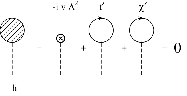
Figure 8: The large-$N_{c}$ tadpole condition for minimizing the Higgs potential.

We proceed by computing the wave-function renormalization constant of the Higgs field, $Z_{h}$, and obtain,

$$Z_{h} = \displaystyle\frac{1}{2}\frac{\kappa}{\kappa_{c}}\left\{c^{2}_{L}s^{2}_{R}\ln\left[\frac{\Lambda^{2}+m_{t}^{2}}{m_{t}^{2}}\right]+(c^{2}_{R}+s^{2}_{L}s^{2}_{R})\ln\left[\frac{\Lambda^{2}+m_{\chi}^{2}}{m_{\chi}^{2}}\right]\right\},$$ (67)

where we have dropped the small ${\cal O}(1)$ constant terms (which are not logarithmically enhanced) together with the tiny ${\cal O}(m_{t}^{2}/M_{\chi}^{2})$ terms. The renormalized $t^{\prime}$-$\overline{t}^{\prime}$-$h$ vertex has Yukawa coupling $c_{L}s_{R}g_{t}/\sqrt{2}$ with $~{}g_{t}=h_{1}/\sqrt{Z_{h}}\,.$ The dynamical mass $m_{t\chi}$ in the seesaw matrix takes the form, $m_{t\chi}=h_{1}v_{0}/\sqrt{2}=g_{t}v/\sqrt{2}$,  which, with Eq. (67), results in a more precise form of the seesaw Pagels-Stokar formula,

$$v^{2} = \frac{m^{2}_{t\chi}}{4\,\pi\,\kappa_{c}}\left\{c^{2}_{L}s^{2}_{R}\ln\left[\frac{\Lambda^{2}+m^{2}_{t}}{m^{2}_{t}}\right]+\left(c^{2}_{R}+s^{2}_{L}s^{2}_{R}\right)\ln\left[\frac{\Lambda^{2}+M^{2}_{\chi}}{M^{2}_{\chi}}\right]\right\}\,.$$ (68)

This equation is an improvement over the previous formula (33) [or (57)] in that the exact seesaw mixing effects associated with the leading logarithmic terms are included. To check the consistency, we note that Eq. (68) reduces back to Eq. (33) under the limit  $(s_{L}^{2},\,s_{R}^{2})\ll 1$ and $m_{t\chi}\approx m_{t}/(\mu_{\chi t}/\mu_{\chi\chi})\approx m_{t}/\sin\theta_{R}$ (where $\sin\theta_{R}\approx\mu_{\chi t}/\mu_{\chi\chi}$). Finally, we note that the above Pagels-Stokar formula is derived under the large-$N_{c}$ fermion bubble approximation, which, for the low scale cutoff $\Lambda\lesssim 10^{4-5}$ GeV, is found to work well in comparison with the full RG evolution (including non-large-$N_{c}$ terms) [28].

2.5 Solutions to the Top Seesaw Gap Equation

In this subsection we present a systematic numerical analysis of the top seesaw gap equations. From the approximate or exact gap equation [cf. Eq. (50) or Eq. (66)], we can see that the seesaw mass gap $m_{t\chi}/\Lambda$ (scaled by $\Lambda$) can be solved as a function of the ${\chi}$-mass parameter $\mu_{\chi\chi}/\Lambda$ (scaled by $\Lambda$), for each given $\kappa/\kappa_{c}$ (the strength of Topcolor gauge force) and the seesaw parameter $r_{t}=(\mu_{\chi t}/\mu_{\chi\chi})^{2}$. Exploring such a relation between $m_{t\chi}/\Lambda$ and $\mu_{\chi\chi}/\Lambda$ will allow us to explicitly examine the behavior of the second order phase transition of the mass gap $m_{t\chi}$ as the ${\chi}$ quark mass scale $\mu_{\chi\chi}$ becomes large. This is shown in Fig. 9 for a typical input of $\kappa/\kappa_{c}=2$ and a wide range of $r_{t}$ values. We have plotted seesaw solutions using both the approximate mass-insertion gap equation (50) and the exact gap equation (66), depicted as dotted and dashed curves in Fig. 9. We see that the two type of solutions indeed converge in the small $m_{t\chi}/\Lambda$ region as expected, and deviate more from each other for larger $m_{t\chi}/\Lambda$ values. As the ratio $\mu_{\chi\chi}/\Lambda$ moves beyond $\sim\!0.63$, the mass gap $m_{t\chi}$ smoothly turns off, indicating a second order phase transition has occurred. In another limit, $\mu_{\chi\chi}/\Lambda\rightarrow 0$, the difference between the two sets of curves becomes the largest as the approximate curves of $m_{t\chi}/\Lambda$ all fall into zero while the exact ones smoothly approach to about $0.63$, a particular solution of the reduced gap equation, $\,1-\kappa_{c}/\kappa=({m_{t\chi}}/{\Lambda})^{2}\ln\left(1+{\Lambda^{2}}/{m^{2}_{t\chi}}\right),\,$ (with $\kappa/\kappa_{c}=2$), derived from Eq. (66) in the limit $\mu_{\chi\chi}/\Lambda\rightarrow 0$.

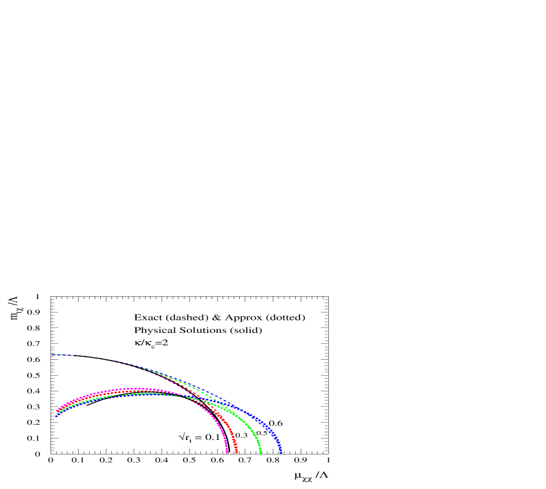
Figure 9: Solutions for top seesaw gap $m_{t\chi}$ with $\kappa/\kappa_{c}=2$ and $\sqrt{r_{t}}=\mu_{\chi t}/\mu_{\chi\chi}=(0.1,\,0.3,\,0.5,\,0.6)$, respectively. The physical seesaw solutions (satisfying $m_{t}=174$ GeV and $v=\sqrt{2}v_{\rm weak}=246$ GeV) are plotted as solid curves, extracted from Fig.( 10). The upper set of curves (dashed curves) are derived from the exact large-$N_{c}$ gap equation (66) and the lower ones (dotted curves) from the mass-insertion gap equation (50).

We now turn to the physical solutions in which we superimpose the requirements of the top mass, $m_{t}=174.3$ GeV, and the full EWSB VEV, $v=246$ GeV. Our strategy is to fix the coloron mass $\Lambda$ (characterizing the Topcolor breaking scale), and the Topcolor gauge coupling at that scale ($h_{1}$, or equivalently, $\kappa/\kappa_{c}$). Then, we are left with three seesaw parameters $(m_{t\chi},\,\mu_{\chi t},\,\mu_{\chi\chi})$ [or, equivalently, $(m_{t\chi},\,r_{t},\,\mu_{\chi\chi})$] to be determined. Indeed, we have three coupled equations to make this determination completely feasible: the gap equation (66) [or (50)], the top mass eigenvalue equation (2.1), and the Pagels-Stokar formula (68) [or, (57)]. From this set of solutions, all other physical quantities, such as the seesaw mixing angles, the mass of ${\chi}$ quark, and the Higgs mass and Yukawa couplings, can be predicted as functions of $\Lambda$ for each given $\kappa/\kappa_{c}$.

In Fig. 10(a)-(c), we present our complete physical seesaw solutions as functions of $\Lambda$ and for various inputs of $\kappa/\kappa_{c}$. For completeness, we also show the prediction of the ${\chi}$ mass ($M_{\chi}$) in Fig. 10(d). Fig. 10(c) shows that the mass gap $m_{t\chi}$ ranges from $\sim\!700$ GeV up to $\sim\!1.7$ TeV for $1.05\leq\kappa/\kappa_{c}\leq 4$, and is quite flat in the entire region of $\Lambda$. There is also a lower limit on the allowed region of $\Lambda$ for each fixed $\kappa/\kappa_{c}$. For instance, $\Lambda$ has to be greater than 1.8 TeV for $\kappa/\kappa_{c}=2$. Furthermore, it is instructive to map our solutions into the plane of $m_{t\chi}/\Lambda$ vs $\mu_{\chi\chi}/\Lambda$ in Fig. 9. Since the seesaw parameters $(m_{t\chi},\,r_{t},\,\mu_{\chi\chi})$ are determined as in Fig. 10(a-c) for each given $\Lambda$ and $\kappa/\kappa_{c}$, we see that the physical solution for $\kappa/\kappa_{c}=2$ (solid curves) indeed take a unique trajectory in the $m_{t\chi}/\Lambda-\mu_{\chi\chi}/\Lambda$ plane of Fig. 9. For $\Lambda$ varying from 1.8 TeV to 80 TeV, the (exact and approximate) physical solutions move from left to right along the two solid curves and fall into good agreement for  $\mu_{\chi\chi}/\Lambda\gtrsim 0.56$ .

With these solutions we are ready to predict physical observables. We first consider the effective $t^{\prime}$-$\overline{t^{\prime}}$-$h$ Yukawa coupling, which can be extracted from Eq. (63),

$$Y_{htt}~{}=~{}g_{t}\,c_{L}s_{R}~{}=~{}\displaystyle\frac{h_{1}}{\sqrt{Z_{h}}}c_{L}s_{R}\,.$$ (69)

In the limit of $r_{t}=(\mu_{\chi t}/\mu_{\chi\chi})^{2}\ll 1$ and $x_{t}=(m_{t\chi}/\mu_{\chi\chi})^{2}\ll 1$, (69) can be approximated as, $Y_{htt}\approx\sqrt{r_{t}}(h_{1}/\sqrt{Z_{h}})$. With the leading order seesaw mass relation, $m_{t}\approx\sqrt{r_{t}}m_{t\chi}=\sqrt{r_{t}}(h_{1}/\sqrt{Z_{h}})(v/\sqrt{2})$,  we arrive at an approximate equation, $Y_{htt}\approx\sqrt{2}m_{t}/v\approx 1$,  as in the SM. Now, we can understand the gross behavior of $Y_{htt}$ in Fig. 11(a). Namely, for the low $\Lambda$ region, the seesaw solutions of $r_{t}$ and $m_{t\chi}/\mu_{\chi\chi}$ are quite sizable [cf. Fig. 10(a-c)] so that the above limit $(r_{t},\,x_{t})\ll 1$ is not good and the deviation $Y_{htt}-1$ is large; also smaller $\kappa/\kappa_{c}$ values have larger $r_{t}$, suggesting larger deviation of $Y_{htt}$ from unity. But, when $\Lambda$ increases, the ratios $(r_{t},\,x_{t})$ drop off quickly and thus $Y_{htt}$ approaches $Y_{htt}=1$.

Other important couplings include the effective $W$-$t^{\prime}$-$b$ and $Z$-$t^{\prime}$-$t^{\prime}$ gauge couplings, which are now modified by the seesaw rotations of $t$ and $\chi$ [cf. Eqs. (29)-(32)]. The $W$-$t^{\prime}$-$b$ coupling $g^{~{}~{}}_{Wtb}$, for instance, involves only the left-handed fields $(t^{\prime}_{L},\,b_{L})$ and we derive,

$$\frac{g^{~{}~{}}_{Wtb}}{g^{\rm SM}_{Wtb}}~{}=~{}c_{L}\,=\,1-\frac{x_{t}}{2(1+r_{t})^{2}}\left[1+\frac{8r_{t}-3}{4(1+r_{t})^{2}}x_{t}\right]+{\cal O}(x_{t}^{3})\,,$$ (70)

where $\,(\sqrt{r_{t}},\,\sqrt{x_{t}})\equiv(\mu_{\chi t},\,m_{t\chi})/\mu_{\chi\chi}\,<\,1$.  We see that the effective coupling $g^{~{}~{}}_{Wtb}$ is reduced from its SM value, and the deviation becomes small in the limit $(r_{t},\,x_{t})\ll 1$ (valid in the large $\Lambda$ region, cf., Fig. 10). This picture is quantitatively shown in Fig. 11(b). Such deviations are important for precision experimental tests at various colliders before the seesaw quark ${\chi}$ can be directly produced.

Finally, we remark that, using the freedom to adjust $r_{t}$ [or equivalently, $\sin\theta$ in Eq. (42)], we can apparently accommodate any fermion mass lighter than $\sim\!700$ GeV. However, this requires some fine-tuning. This freedom may be useful in constructing more complete models involving all three generations. The top quark is unique, however, in that its large mass is very difficult to accommodate in any other way, and there is less apparent fine-tuning. We therefore believe it is generic, in any model of this kind, that the top quark receives the bulk of its mass through this seesaw mechanism.

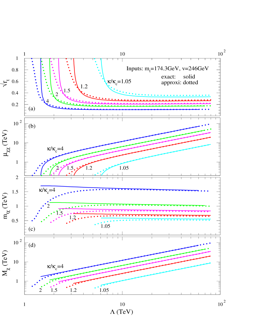
Figure 10: Solutions of the top seesaw gap equations are shown in plots (a)-(c) for $\kappa/\kappa_{c}=(1.2,\,1.5,\,2,\,4)$, with $m_{t}=174.3$ GeV and $v=\sqrt{2}v_{\rm weak}=246$ GeV superimposed. The solid curves are derived from the exact gap equation (66) while the dotted curves from the mass-insertion gap equation (50). The predicted physical mass-eigenvalue of ${\chi}$ quark is also shown in the plot (d).

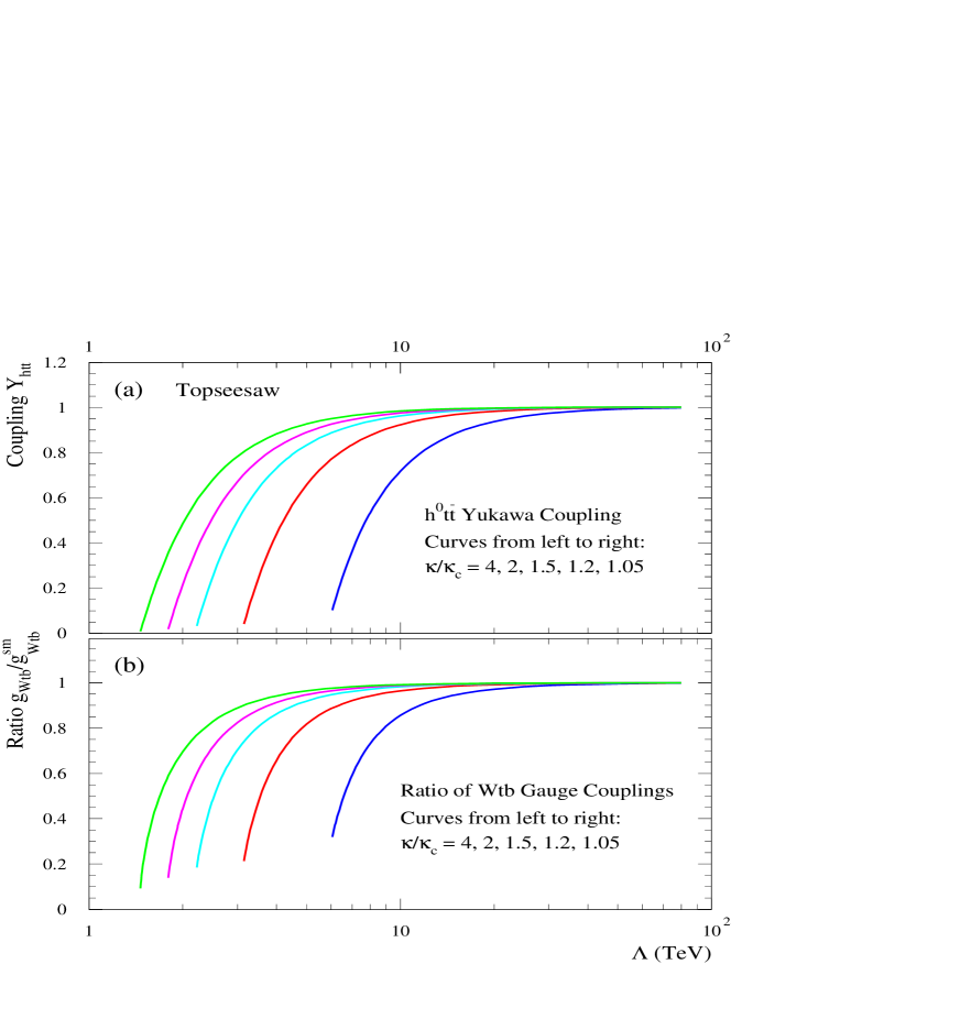
Figure 11: The predicted effective Higgs Yukawa coupling $Y_{htt}$ in (a), and $W$-$t$-$b$ gauge coupling $g_{Wtb}$ shown as the ratio over its SM value in (b).

2.6 The Composite Higgs Boson Mass

With the seesaw gap equation solved in the previous subsection, we can proceed to analyze the mass spectrum of the composite Higgs boson. From Eqs. (62), (64) and (67), and taking the usual large-$N_{c}$ fermion-bubble approximation, we can straightforwardly compute the physical Higgs boson mass $M_{h}$. A lengthy calculation gives,

$$\begin{array}[]{ll}M_{h}^{2}=&\!\!\!\displaystyle\frac{1}{Z_{h}}\left\{\left(1-\frac{\kappa}{\kappa_{c}}\right)\Lambda^{2}\right.\\[17.07164pt] &\displaystyle+\frac{\kappa}{\kappa_{c}}\left[\left(3s_{L}^{2}c_{R}^{2}+\left(c_{L}^{2}c_{R}^{2}+s_{L}^{2}s_{R}^{2}\right)\frac{M_{\chi}^{2}}{M_{\chi}^{2}-m_{t}^{2}}+2c_{L}c_{R}s_{L}s_{R}\frac{M_{\chi}m_{t}}{M_{\chi}^{2}-m_{t}^{2}}\right)M_{\chi}^{2}\ln\left(\frac{\Lambda^{2}}{M_{\chi}^{2}}+1\right)\right.\\[17.07164pt] &\displaystyle\hskip 19.91692pt+\left(3c_{L}^{2}s_{R}^{2}-\left(c_{L}^{2}c_{R}^{2}+s_{L}^{2}s_{R}^{2}\right)\frac{m_{t}^{2}}{M_{\chi}^{2}-m_{t}^{2}}-2c_{L}c_{R}s_{L}s_{R}\frac{M_{\chi}m_{t}}{M_{\chi}^{2}-m_{t}^{2}}\right)m_{t}^{2}\ln\left(\frac{\Lambda^{2}}{m_{t}^{2}}+1\right)\\[17.07164pt] &\displaystyle\left.\left.\hskip 19.91692pt-2s_{L}^{2}c_{R}^{2}\frac{\Lambda^{2}M_{\chi}^{2}}{\Lambda^{2}+M_{\chi}^{2}}-2c_{L}^{2}s_{R}^{2}\frac{\Lambda^{2}m_{t}^{2}}{\Lambda^{2}+m_{t}^{2}}\right]\right\}\,.\end{array}$$ (71)

To compare with Eq. (58), we consider the limit $r_{t}\equiv(\mu_{\chi t}/\mu_{\chi\chi})^{2}\rightarrow 0$ and expand all quantities in terms of the small parameter $x_{t}\equiv(m_{t\chi}/\mu_{\chi\chi})^{2}$, so that, $(m_{t},\,M_{\chi})\approx\left(0,\,\mu_{\chi\chi}\sqrt{1+x_{t}}\right)$ and $(s_{L},s_{R})\approx(x_{t},\,0)$.  With these, we verify that the $M_{h}^{2}$ formula (71) reduces to $\,M_{h}\approx 2m_{t\chi}$,  in agreement with the approximate mass relation (58) derived by the gauge-invariant RG analysis. Using the physical seesaw solutions [cf. Fig. 10(a)-(c)], we can plot the predicted Higgs mass from Eq. (71) [Eq. (58)] as the solid [dotted] curves in Fig. 12(a). It is important to note that our current large-$N_{c}$ fermion-bubble approximation predicts a heavy Higgs mass, typically around $1$ TeV , saturating the SM unitarity bound.

When the ratio $\kappa/\kappa_{c}$ becomes closer to one (i.e., $\kappa$ becomes more critical), the Higgs mass becomes lighter, as expected from the mass formula (71). Also, the approximate relation $M_{h}\approx 2m_{t\chi}$ in (58) holds better for smaller $\kappa/\kappa_{c}\sim 1$ (to about $30\%$) and becomes less reliable for larger $\kappa/\kappa_{c}$ value with an overestimate factor up to $\sim\!2$. This shows that the current improved broken phase calculation of $M_{h}$ (including exact seesaw mixings) already works better than the usual approach which results in $M_{h}\approx 2m_{t\chi}$ [9, 17, 29].

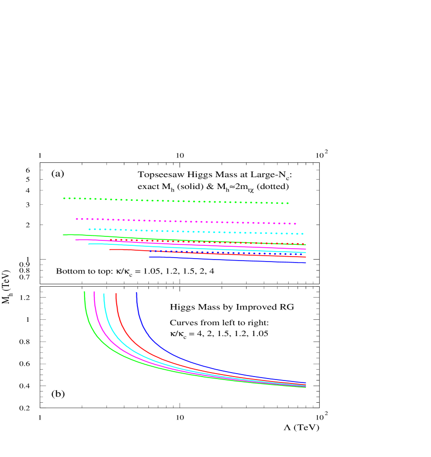
Figure 12: The predicted mass spectrum of the top seesaw Higgs boson: (a) by the large-$N_{c}$ fermion-bubble calculation; and (b) by an improved RG analysis including the Higgs self-coupling evolution.

Finally, we note that the above calculation of the Higgs mass $M_{h}$ includes only the large-$N_{c}$ fermion-bubble contributions, but ignores the non-large-$N_{c}$ Higgs propagation in the loop. For the leading logarithmic terms in $M_{h}$, this corresponds to solving the RG equations (RGEs) for top Yukawa coupling ($y_{t}$) and Higgs self-coupling ($\lambda$) by keeping the fermion-bubble terms. This approach also applies to the calculation of top mass $m_{t}$ and results in the Pagels-Stokar formula which, in the case of a low cutoff scale $\Lambda\sim 10^{4-5}$ GeV, is found to agree well with the full RG evolution. In the minimal top-condensate model [15], the large-$N_{c}$ fermion-bubble calculation of $m_{t}$ agrees with full RG analysis to $5-14\%\,(34\%)$ level for $\Lambda=10^{5-4}\,(10^{19})\,$GeV, while for the Higgs mass prediction, the former tends to overestimate $M_{h}$ by a factor of $1.8-2\,(1.2)$ for $\Lambda=10^{5-4}\,(10^{19})\,$GeV [28]. This is due to the fact that for a high scale $\Lambda$, $m_{t}$ is controlled by the infrared quasi-fixed point [21]; for a low scale $\Lambda$, the infrared fixed point is not reached and the $m_{t}$ value is mainly determined by the dominant large-$N_{c}$ RG running so that the fermion-bubble calculation works well [28].

The Higgs mass in the case of a high scale $\Lambda$ is again controlled by the infrared quasi-fixed point (where the $y_{t}$-term and $\lambda$-term tend to cancel in the $\beta$-function of $\lambda$); however, the situation with a low scale $\Lambda$ is different as the infrared fixed point is not reached and the positive (non-large-$N_{c}$) $\lambda^{2}$-term in the $\beta$-function of $\lambda$ has a sizable numerical coefficient compared to the negative large-$N_{c}$ $y_{t}^{4}$-term. This $\lambda^{2}$-term can drive $\lambda$ (and thus $M_{h}$) to lower value and corrects the usual fermion-bubble calculation by a factor $\sim\!1.8-2$ for $\Lambda=10^{4-5}$ GeV [15, 28], but, the uncertainties of the one-loop RG predictions (from the unknown non-perturbative dynamics associated with the compositeness condition at $\mu=\Lambda$) also become much larger, of ${\cal O}(100-200)$ GeV [15], as the infrared fixed point is not so relevant. Hence, the one-loop full RG analysis (with compositeness conditions) [15] may not be more reliable than the usual fermion-bubble calculation for theories with a low scale $\Lambda$. Similar features should hold for the $M_{h}$ analysis in the top seesaw model [except a complication by the new mass scale $M_{\chi}$ between $(m_{t},\,M_{h})$ and $\Lambda$]. Nevertheless, we feel it is useful to implement such an improved one-loop RG analysis of $M_{h}$ below (in the spirit of Ref. [15]), as a comparison.

Using the mass-independent $\overline{\rm MS}$ scheme [15], we consider the top-seesaw RG evolution in two steps: (i). for the range $\Lambda\geq\mu\geq M_{\chi}$; (ii). for the range $M_{\chi}\geq\mu\geq(M_{h},\,m_{t})$. We start with the gauge-invariant effective Lagrangian (52) at $\mu=\Lambda$,

$${\cal{L}}_{\Lambda}={\cal{L}}_{\rm kinetic}-\left[\,\mu_{\chi t}\,\overline{{\chi}_{L}}t_{R}+\mu_{\chi\chi}\,\overline{\chi_{R}}\,\chi_{L}+h_{\rm 1}\,\overline{\psi_{L}}\,{\chi}_{R}\,\Phi_{0}+{\rm h.c.}\right]-\Lambda^{2}\Phi_{0}^{\dagger}\Phi_{0}\,,$$ (72)

where for simplicity the partial rotation (42) is not taken since we will use a mass-independent RG scheme [15] and consider $M_{\chi}\simeq\mu_{\chi\chi}$. For $\Lambda>\mu\geq M_{\chi}$, the effective Lagrangian ${\cal{L}}_{M_{\chi}\leq\mu<\Lambda}$ contains,

$$\begin{array}[]{l}-\left(\,\mu_{\chi t}\,\overline{{\chi}_{L}}t_{R}+\mu_{\chi\chi}\,\overline{\chi_{R}}\,\chi_{L}+h_{\rm 1}\,\overline{\psi_{L}}\,{\chi}_{R}\,\Phi_{0}+{\rm h.c.}\right)+Z_{\Phi}\left|D\Phi_{0}\right|^{2}-\widetilde{M}_{\Phi}^{2}(\mu)\Phi_{0}^{\dagger}\Phi_{0}-\widetilde{\lambda}\left(\Phi_{0}^{\dagger}\Phi_{0}\right)^{2}\\[11.38109pt] =-\left(\,\mu_{\chi t}\,\overline{{\chi}_{L}}t_{R}+\mu_{\chi\chi}\,\overline{\chi_{R}}\,\chi_{L}+g_{t}\,\overline{\psi_{L}}\,{\chi}_{R}\,\Phi+{\rm h.c.}\right)+\left|D\Phi\right|^{2}-{M}_{\Phi}^{2}(\mu)\Phi^{\dagger}\Phi-{\lambda}\left(\Phi^{\dagger}\Phi\right)^{2}\,,\end{array}$$ (73)

where $g_{t}=h_{1}/Z_{\Phi}^{1/2}$, $M_{\Phi}^{2}=\widetilde{M}_{\Phi}^{2}/Z_{\Phi}$, and $\lambda=\widetilde{\lambda}/Z_{\Phi}^{2}$, with $Z_{\Phi}(\mu)\simeq(\kappa/\kappa_{c})\ln\left(\Lambda/\mu\right)\,$ and $\widetilde{\lambda}(\mu)\simeq 4\pi^{2}(\kappa^{2}/\kappa_{c})\ln\left(\Lambda/\mu\right)\,$ in the $\overline{\rm MS}$ scheme. The SM gauge couplings are negligible for the current analysis and we can write the RGE of $\lambda$ in the region $\Lambda\geq\mu\geq M_{\chi}$,

$$\beta(\lambda)=\displaystyle\frac{d\lambda}{d\ln\mu}\simeq\displaystyle\frac{1}{8\pi^{2}}\left[-N_{c}g_{t}^{4}+2N_{c}\lambda g_{t}^{2}+12\lambda^{2}\right],$$ (74)

where the $\lambda$-terms on the right-hand side tend to decrease $\lambda$ (and $M_{h}$) and are ignored in the usual fermion-buble calculation (which is justified for $g_{t}^{2}\gg\lambda$ and $N_{c}\gg 1$). The large-$N_{c}$ relation $g_{t}=h_{1}/Z_{\Phi}^{1/2}$ gives the $\psi$-$\chi$-$\Phi$ Yukawa coupling,

$$g_{t}^{2}(\mu)\,\simeq\,\frac{8\pi^{2}/N_{c}}{\ln(\Lambda/\mu)}\gg 1\,,$$ (75)

which suggests the compositeness boundary condition $g_{t}^{2}(\Lambda)=\infty$. The complete large-$N_{c}$ RGE for $g_{t}$ is,

$$\frac{dg^{2}_{t}}{d\ln\mu}=\frac{1}{8\pi^{2}}\left[N_{c}g_{t}^{2}-3\frac{N_{c}^{2}-1}{N_{c}}g_{3}^{2}\right]g_{t}^{2}\,,$$ (76)

where the effect of the QCD coupling $g_{3}$ is found to be numerically negligible for the current analysis, so that $g_{t}^{2}$ may be solved analytically,

$$g^{2}_{t}(\mu)\simeq\left[g_{t}^{-2}(\Lambda)+\frac{N_{c}}{8\pi^{2}}\ln\frac{\Lambda}{\mu}\right]^{-1}.$$ (77)

The boundary value $\lambda(\Lambda)$ may be estimated using the above large-$N_{c}$ fermion-bubble relation $\lambda=\widetilde{\lambda}/Z_{\Phi}^{2}$, corresponding to keeping the first term on the right-hand side of the RGE (74), i.e.,

$$\lambda(\mu)\simeq\left[g_{t}^{-2}(\Lambda)+\frac{N_{c}}{8\pi^{2}}\ln\frac{\Lambda}{\mu}\right]^{-1}\,,$$ (78)

from which, we define the compositeness conditions at $\mu=\Lambda$,

$$\lambda(\Lambda)=g_{t}^{2}(\Lambda)=\infty\,.$$ (79)

Using this and (77), we can solve the complete RGE (74) and deduce $\lambda(M_{\chi})$. As $\mu$ approaches the scale $M_{\chi}$, we perform the partial diagonalization (42) to the mass terms in Eq. (73) and then decouple ${\chi}$ at $\mu\leq M_{\chi}$. This gives the effective Lagrangian (55) derived earlier, with $\overline{M}\simeq M_{\chi}$ and the renormalized $t$-$t$-$\Phi$ Yukawa coupling $y_{t}(\mu)=g_{t}(\mu)\sin\theta$ for $\mu\leq M_{\chi}$. The on-shell condition $m_{t}(m_{t})=y_{t}(m_{t})v/\sqrt{2}=174$ GeV requires $y_{t}(m_{t})\simeq 1$, so that $y_{t}(\mu)$ is constrained to be small, close to $1$,

$$y^{2}_{t}(\mu)\simeq\left[1-\frac{N_{c}}{8\pi^{2}}\ln\frac{\mu}{m_{t}}\right]^{-1}\gtrsim 1\,,~{}~{}~{}~{}~{}~{}(\mu\leq M_{\chi})\,.$$ (80)

The numerical effect of $y_{t}(\mu)$ on the relevant $\lambda$ running is found to be small for $\mu\in\left(M_{h},\,M_{\chi}\right)$. Thus, the step-(ii) RG evolution of $\lambda$ in the region $M_{\chi}\geq\mu\geq M_{h}$ is essentially controlled by the simplified RGE, $d\lambda/d\ln\mu\simeq 3\lambda^{2}/2\pi^{2}$. The physical Higgs mass is then numerically solved from the on-shell condition,

$$M_{h}^{2}=2v^{2}\lambda(M_{h})\simeq\displaystyle{2}v^{2}\left[{\displaystyle\frac{1}{\lambda(M_{\chi})}+\frac{3}{4\pi^{2}}\ln\frac{M_{\chi}^{2}}{M_{h}^{2}}}\,\right]^{-1},$$ (81)

and is plotted in Fig. 12(b).

Since the ${\chi}$ mass $M_{\chi}$ is determined from solving the seesaw gap equation for each given $\Lambda$ and $\kappa/\kappa_{c}$ in Sec. 2.5, Fig. 12(b) shows different Higgs mass spectrua as $\kappa/\kappa_{c}$ varies. We see that for $\Lambda<10$ TeV, $M_{h}$ ranges around $(0.7-1.25)\,{\rm TeV}\sim\!1$ TeV, while for $\Lambda\gtrsim 10$ TeV the $\lambda$ running becomes more significant, bringing $M_{h}$ down to $\sim\!650-400$ GeV which is about a factor 2 below the large-$N_{c}$ fermion-bubble calculation in Fig. 12(a), as also expected from the analysis of the minimal top-condensate model [15, 28]. However, we must note that for dynamical symmetry breaking theories with a low scale cutoff $\Lambda\sim 10-100$ TeV, the infrared fixed point becomes less relevant and the uncertainties in $M_{h}$ associated with the compositeness condition (79) are large, around ${\cal O}(100-200)$ GeV, so that the naive one-loop RG running is not so reliable and higher loop corrections could be important as well. Furthermore, the simplest mass-independent $\overline{\rm MS}$ RG scheme may have its drawback in treating such low scale dynamical theories, in comparison with the mass-dependent renormalization [30] which suggests that the large Higgs mass nearby $\Lambda$ will suppress $\lambda$ running and result in higher $M_{h}$ values [31, 16]. Hence, the RG improved spectrum in Fig. 12(b) only serves as a reference to show how the traditional large-$N_{c}$ fermion-bubble calculation in the top seesaw model might be improved when including the perturbative Higgs self-coupling evolution.

3 Extensions with Bottom Quark

3.1 The Mechanism for Bottom Quark Mass

As things stand, we have not addressed the issue of the bottom quark mass. The simplest way of producing the $b$ quark mass is to include additional weak-singlet fermionic fields $\omega_{L}$ and $\omega_{R}$ together with $b_{R}$, which are charged under the gauge group $SU(3)_{1}\otimes SU(3)_{2}\otimes SU(2)_{W}\otimes U(1)_{Y}$,

$$b_{R},\omega_{L}\!:~{}\,\left({\bf 1,3,1,}-\frac{2}{3}\right)\,,~{}~{}~{}~{}~{}~{}\omega_{R}:~{}\,\left({\bf 3,1,1,}-\frac{2}{3}\right)\,.$$ (82)

Such assignments for the $b-{\omega}$ sector nicely cancel the unwanted gauge-anomalies from the Top Seesaw sector (cf. Sec. 2.1), so that we can regard their presence as a generic part of the standard Topcolor picture. We further allow $\overline{\omega}_{L}\omega_{R}$ and $\overline{\omega}_{L}b_{R}$ mass terms, in addition to the $\chi-t$ mass terms [cf. the Eq. (39) in Sec. 2.2],

$${\cal{L}}_{\rm mass}~{}=\,-\left(\mu_{\chi\chi}\,\overline{\chi_{L}}\,\chi_{R}\,+\,\mu_{\chi t}\,\overline{\chi_{L}}\,t_{R}\right)-\left(\mu_{\omega\omega}\,\overline{\omega_{L}}\omega_{R}\,+\,\mu_{\omega b}\,\overline{\omega_{L}}b_{R}\right)\,+\,{\rm h.c.}\,.$$ (83)

With the previous assignments for the $\chi$ quarks, the extended model can be schematically represented as below,

$\ \ \ \ \ \ \ \ \ \ \ \ ~{}\,SU(3)_{1}$                  $\ \ \ \ \ SU(3)_{2}$            

$\left\lgroup\begin{array}[]{c}\left(\!\begin{array}[]{c}t_{L}\\ b_{L}\end{array}\!\right)~{}~{}I=\frac{1}{2}\\[19.91692pt] \left(\!\begin{array}[]{c}\chi_{R}\\ \omega_{R}\end{array}\!\right)~{}~{}I=0\end{array}\right\rgroup$     $\left\lgroup\begin{array}[]{c}\left(\!\begin{array}[]{c}t_{R}\\ b_{R}\end{array}\!\right)~{}~{}I=0\\[19.91692pt] \left(\!\begin{array}[]{c}\chi_{L}\\ \omega_{L}\end{array}\!\right)~{}~{}I=0\end{array}\right\rgroup$

We see that the additional quark ${\omega}_{R}$ joins the strong Topcolor $SU(3)_{1}$ like ${\chi}_{R}$. After the Topcolor breaking and integrating out massive colorons, we have following NJL interactions,

$${\cal L}_{\rm int} = \frac{h_{1}^{2}}{\Lambda^{2}}\;\left[\left(\bar{\psi}_{L}\chi_{R}\right)\left(\bar{\chi}_{R}\psi_{L}\right)+\left(\bar{\psi}_{L}\omega_{R}\right)\left(\bar{\omega}_{R}\psi_{L}\right)\right]$$ (84)

$$\rightarrow -\Lambda^{2}\left(\Phi_{t0}^{\dagger}\;\Phi_{t0}+\Phi_{b0}^{\dagger}\;\Phi_{b0}\right)-h_{1}\,\left(\bar{\psi}_{L}\;\Phi_{t0}\;\chi_{R}+\bar{\psi}_{L}\;\Phi_{b0}\;\omega_{R}\right)+{\rm h.c.}\,,$$

which contains two scalar doublets $\Phi_{t0}$ and $\Phi_{b0}$ after the bosonization of the NJL vertices. The Lagrangian ${\cal L}_{\rm mass}+{\cal L}_{\rm int}$, however, poses a global $U(1)$ symmetry under which the fields transform as,

$$\begin{array}[]{llll}\psi_{L}\rightarrow\psi_{L}\,,&t_{R}\rightarrow e^{i\alpha}\,t_{R}\,,&b_{R}\rightarrow e^{i\alpha}\,b_{R}\,,&\\[5.69054pt] {\chi}_{L(R)}\rightarrow e^{i\alpha}\,{\chi}_{L(R)}\,,&{\omega}_{L(R)}\rightarrow e^{i\alpha}\,{\omega}_{L(R)}\,,&{\Phi}_{t0}\rightarrow e^{-i\alpha}\,{\Phi}_{t0}\,,&{\Phi}_{b0}\rightarrow e^{-i\alpha}\,{\Phi}_{b0}\,.\end{array}$$ (85)

If this symmetry were exact, the dynamical condensates $\langle\overline{t_{L}}{\chi}_{R}\rangle$ and $\langle\overline{b_{L}}{\omega}_{R}\rangle$ (or, equivalently, the scalar VEVs $\langle\Phi_{t0}\rangle$ and $\langle\Phi_{b0}\rangle$) would spontaneously break it and generate a problematic massless Goldstone boson (the Peccei-Quinn axion). Fortunately, the symmetry is anomalous, and the Topcolor instanton effect [7] induces an effective Peccei-Quinn breaking term via the ’t Hooft flavor determinant [37] with the form,

$$\frac{c_{0}}{\Lambda^{2}}\det\left[\overline{\psi_{L}}\left(\begin{array}[]{c}{\chi}_{R}\\[5.69054pt] {\omega}_{R}\end{array}\right)\right]\,+\,{\rm h.c.}~{}=~{}\displaystyle\frac{c_{0}}{\Lambda^{2}}\epsilon^{\alpha\beta}\left(\overline{\psi_{L}}^{\alpha}{\chi}_{R}\right)\left(\overline{\psi_{L}}^{\beta}{\omega}_{R}\right)\,+\,{\rm h.c.}\,,$$ (86)

where $c_{0}$ is a (complex) constant depending on details of the Topcolor strong dynamics and from experience with QCD we expect, $c_{0}\sim{\cal O}(0.1-1)$. In analogy with the $\eta^{\prime}$ in QCD, this effective interaction will provide a non-zero mass for the axionic pseudo-Goldstone boson. It is also possible that such an effective Peccei-Quinn breaking term may also arise from additional flavor dynamics at a scale much above the Topcolor breaking scale [17]. In general, we parametrize the Peccei-Quinn breaking interaction as,

$${\cal L}_{{\rm PQB}} = \frac{\xi\,h^{2}_{1}}{\Lambda^{2}}\epsilon^{\alpha\beta}\left[\left(\overline{\chi_{R}}\;\psi_{L}^{\alpha}\right)\left(\overline{\omega_{R}}\;\psi_{L}^{\beta}\right)+\left(\overline{\psi_{L}}^{\alpha}\chi_{R}\right)\left(\overline{\psi_{L}}^{\beta}\omega_{R}\right)\right]$$ (87)

$$\rightarrow -\xi\;\epsilon^{\alpha\beta}\left[\Lambda^{2}\Phi_{t0}^{\alpha}\;\Phi_{b0}^{\beta}+h_{1}\left(\overline{\chi_{R}}\;\psi^{\alpha}_{L}\;\Phi_{b0}^{\beta}+\overline{\omega_{R}}\;\psi^{\beta}_{L}\;\Phi_{t0}^{\alpha}\right)\right]\,+\,{\rm h.c.}\,.$$

where we ignore a possible phase in the parameter $\xi$ and let it be real for the purpose of the current study. With the Topcolor instantons as the origin of this effective interaction, we can estimate the typical size of $\xi$,

$$\xi=c_{0}/h_{1}^{2}=c_{0}\left[\displaystyle\frac{8\pi^{2}}{3}\frac{\kappa}{\kappa_{c}}\right]^{-1}\sim{\cal O}(10^{-2}-10^{-3})\,,$$ (88)

where $c_{0}\sim{\cal O}(0.1-1)$ and $\kappa/\kappa_{c}\sim 2-4$. Since the relevant values of $\xi$ are tiny, it is justified to treat it as a perturbation and only include the corrections up to ${\cal O}(\xi^{1})$. We note that, in addition to generating an explicit axion mass, the above interaction (87) also provides a correction to the mass terms  $m_{t\chi}\overline{t_{L}}{\chi}_{R}$  and  $m_{b\omega}\overline{b_{L}}{\omega}_{R}$,  i.e., we generally have, from (84) and (87),

$$m_{t\chi}\,=\,\displaystyle h_{1}\left(\langle\Phi_{t0}\rangle+\xi\langle\Phi_{b0}\rangle\right)\,,~{}~{}~{}~{}~{}m_{b\omega}\,=\,\displaystyle h_{1}\left(\langle\Phi_{b0}\rangle+\xi\langle\Phi_{t0}\rangle\right)\,.$$ (89)

The second equation gives the physical $b$ mass, $m_{b}\approx m_{b\omega}\mu_{\omega b}/\mu_{\omega\omega}$, via the following seesaw matrix,

$$-\left(\overline{b_{L}}~{}~{}\overline{{\omega}_{L}}\right)\left\lgroup\begin{array}[]{cc}0&m_{b{\omega}}\\[5.69046pt] \mu_{\omega b}&\mu_{\omega\omega}\\ \end{array}\right\rgroup\left(\!\!\begin{array}[]{c}b_{R}\\ {\omega}_{R}\end{array}\!\!\right)\,+\,{\rm h.c.}\,.$$ (94)

For $\xi\gtrsim 10^{-2}$, there is the interesting possibility that the $b$ mass may completely originate from ${\cal L}_{\rm PQB}$ (for example, from Topcolor instanton effects). This requires $\langle\Phi_{b0}\rangle=0$, implying the leading order Lagrangian (84) to have a zero mass-gap in the $\left(\overline{b_{L}}{\omega}_{R}\right)$ channel which can be realized when ${\omega}$ becomes very heavy ($\mu_{\omega\omega}\gg\Lambda$) and decouples. In this special case, the whole model reduces back to our minimal top seesaw model studied in Sec. 2, except that now the $b$ quark acquires its mass from Topcolor instantons,

$$m_{b}\approx m_{b\omega}\mu_{\omega b}/\mu_{\omega\omega}\,,~{}~{}~{}~{}~{}\left(\;{\rm with}~{}m_{b\omega}=\xi h_{1}\langle\Phi_{t0}\rangle=\xi m_{t\chi}\;\right)\,.$$ (95)

Consequently, the Higgs doublet $\Phi_{b0}$ is also removed from the low energy theory and the remaining analysis of this decoupling limit becomes identical to Sec. 2. However, in the more general cases where ${\omega}$ does not decouple from the theory ( $\mu_{\omega\omega}\!\lesssim\!\Lambda$ ), the $b$ quark can acquire its mass from both terms in the second relation of (89); and furthermore, for $\xi\lesssim 10^{-3}$ and $\mu_{\omega b}/\mu_{\omega\omega}\lesssim 1$, the mass $m_{b}$ predominantly comes from the leading order term. Such non-decoupling scenarios also have a rich physical Higgs spectrum as both Higgs doublets (including the massive axion) will be accessible in our low energy theory. These will be systematically studied below.

3.2 Gap Equations for Top and Bottom Seesaws and the Physical Solutions

In this subsection, we derive the gap equations for both top and bottom seesaws up to ${\cal O}(\xi)$ and analyze their physical solutions. This is in analogy with Sec. 2.4, but with the $b$ seesaw mass gap and ${\cal O}(\xi)$ corrections included. We start by explicitly defining the bare fields of the two Higgs doublets $\Phi_{t0}$ and $\Phi_{b0}$ in the shifted vacuum,

$${\Phi}_{t0}\,=\,\left(\!\begin{array}[]{c}\left(v_{t0}+h_{t0}^{0}+i\pi^{0}_{t0}\right)/\sqrt{2}\\[8.53581pt] \pi^{-}_{t0}\end{array}\!\right),~{}~{}~{}~{}~{}~{}{\Phi}_{b0}\,=\,\left(\!\begin{array}[]{c}\pi^{+}_{b0}\\[8.53581pt] \left(v_{b0}+h_{b0}^{0}+i\pi^{0}_{b0}\right)/\sqrt{2}\end{array}\!\right),$$ (96)

where, as in usual 2-Higgs-doublet model (2HDM) and upon renormalization, the rotations of $h_{t}^{0}$ and $h_{b}^{0}$ give the mass-eigenstates of neutral Higgs bosons $(h^{0},\,H^{0})$, while the combinations of other six scalars $\pi_{t}^{0,\pm}$ and $\pi_{b}^{0,\pm}$ result in three would-be Goldstone bosons (eaten by $W^{\pm},Z^{0}$) and three physical Higgs states $(A^{0},\,H^{\pm})$. Now, we can explicitly write the two seesaw mass-gaps in (89) as,

$$m_{t\chi}=\frac{h_{1}}{\sqrt{2}}\left(v_{t0}+\xi v_{b0}\right)\,,~{}~{}~{}~{}~{}m_{b\omega}=\frac{h_{1}}{\sqrt{2}}\left(v_{b0}+\xi v_{t0}\right)\,.$$ (97)

In the same spirit of Sec. 2.4 and using the Lagrangian $\,{\cal L}_{\rm mass}+{\cal L}_{\rm int}+{\cal L}_{\rm PQB}$,  we obtain two coupled gap equations up to $O(\xi)$ from the tadpole conditions of the neutral Higgs fields $h_{t0}^{0}$ and $h_{b0}^{0}$, as shown in Fig. 13. Thus, we can derive them as,

$$m_{t\chi}\,=\,\displaystyle\frac{\kappa}{\kappa_{c}}\left[F_{t}+\xi F_{b}\right]\,,~{}~{}~{}~{}~{}~{}m_{b\omega}\,=\,\displaystyle\frac{\kappa}{\kappa_{c}}\left[F_{b}+\xi F_{t}\right]\,,$$ (98)

or, equivalently, up to ${\cal O}(\xi)$,

$$\frac{\kappa}{\kappa_{c}}(m_{t\chi}-\xi m_{b\omega})\,=\,F_{t}\,,~{}~{}~{}~{}~{}~{}\displaystyle\frac{\kappa}{\kappa_{c}}(m_{b\omega}-\xi m_{t\chi})\,=\,F_{b}\,,$$ (99)

where

$$\begin{array}[]{lll}F_{t}&=&\displaystyle c^{t}_{L}s^{t}_{R}\left(m_{t}-\frac{m_{t}^{3}}{\Lambda^{2}}\ln\left[\frac{\Lambda^{2}+m_{t}^{2}}{m_{t}^{2}}\right]\right)+s^{t}_{L}c^{t}_{R}\left(M_{\chi}-\frac{M_{\chi}^{3}}{\Lambda^{2}}\ln\left[\frac{\Lambda^{2}+M_{\chi}^{2}}{M_{\chi}^{2}}\right]\right)\,,\\[14.22636pt] F_{b}&=&\displaystyle c^{b}_{L}s^{b}_{R}\left(m_{b}-\frac{m_{b}^{3}}{\Lambda^{2}}\ln\left[\frac{\Lambda^{2}+m_{b}^{2}}{m_{b}^{2}}\right]\right)+s^{b}_{L}c^{b}_{R}\left(M_{\omega}-\frac{M_{\omega}^{3}}{\Lambda^{2}}\ln\left[\frac{\Lambda^{2}+M_{\omega}^{2}}{M_{\omega}^{2}}\right]\right)\,,\end{array}$$ (100)

and the seesaw rotation angles $s_{L,R}^{t,b}$ and $c_{L,R}^{t,b}$ are similarly defined as in Eqs. (29)-(32). We see that the two gap equations decouple from each other at the leading order ${\cal O}(\xi^{0})$ and the correlations appear at ${\cal O}(\xi)$ which are generally small. The ${\cal O}(\xi)$ terms become important only for very large $\tan\beta=v_{t}/v_{b}$ and sizable $\xi\gtrsim 10^{-2}$. For instance, a typical case with $\tan\beta=40$ and $\xi=2\times 10^{-2}$ gives the ratio $(\xi v_{t})/v_{b}=80\%$, implying that the $\xi$-term makes up about $80\%$ of the mass-gap $m_{b\omega}$ and thus the $b$ mass. Another important role of the ${\cal O}(\xi)$ interactions is their contributions to the Higgs masses, especially, the mass of the pseudo-scalar $A^{0}$.

Similar to the RG analysis in Sec. 2.4, we can further evolve the Higgs Lagrangian $\,{\cal L}_{\rm mass}+{\cal L}_{\rm int}+{\cal L}_{\rm PQB}$,  from the scale $\Lambda$ down to $\mu\left(<\mu_{{\chi}{\chi},{\omega}{\omega}}\leq\Lambda\right)$ by integrating out loops with the heavy fermions $({\chi},\,{\omega})$. The Higgs fields get renormalized, e.g., $h_{t0}^{0}=Z_{ht}^{1/2}h_{t}^{0},\,h_{b0}^{0}=Z_{hb}^{1/2}h_{b}^{0},\,$ and so on. We can write down the renormalized Higgs VEVs, $v_{t}=Z_{h_{t}}^{1/2}v^{0}_{t}$ and $v_{b}=Z_{h_{b}}^{1/2}v^{0}_{b}$, and define their ratio, $\tan\beta=v_{t}/v_{b}$, as usual. Here, the two neutral Higgs wave-function renormalization constants are computed as,

$$\begin{array}[]{lll}Z_{h_{t}}&=&\displaystyle\frac{1}{2}\frac{\kappa}{\kappa_{c}}\left\{c^{t\,2}_{L}s^{t\,2}_{R}\ln\left[\frac{\Lambda^{2}+m_{t}^{2}}{m_{t}^{2}}\right]+(c^{t\,2}_{R}+s^{t\,2}_{L}s^{t\,2}_{R})\ln\left[\frac{\Lambda^{2}+m_{\chi}^{2}}{m_{\chi}^{2}}\right]\right\}+{\cal O}(\xi^{2})\,,\\[14.22636pt] Z_{h_{b}}&=&\displaystyle\frac{1}{2}\frac{\kappa}{\kappa_{c}}\left\{c^{b\,2}_{L}s^{b\,2}_{R}\ln\left[\frac{\Lambda^{2}+m_{b}^{2}}{m_{b}^{2}}\right]+(c^{b\,2}_{R}+s^{b\,2}_{L}s^{b\,2}_{R})\ln\left[\frac{\Lambda^{2}+m_{\omega}^{2}}{m_{\omega}^{2}}\right]\right\}+{\cal O}(\xi^{2})\,,\end{array}$$ (101)

in which the $\xi$-corrections appear only at ${\cal O}(\xi^{2})$ as can be seen from the interaction Lagrangian ${\cal L}_{\rm int}+{\cal L}_{\rm PQB}$. Then, from Eqs. (89) and (101), we derive two new Pagels-Stokar formulae,

$$\begin{array}[]{lll}v_{t}^{2}&=&\displaystyle\frac{\left(m_{t\chi}-\xi m_{b\omega}\right)^{2}}{4\,\pi\,\kappa_{c}}\left\{c^{t\;2}_{L}s^{t\;2}_{R}\ln\left[\frac{\Lambda^{2}+m^{2}_{t}}{m^{2}_{t}}\right]+\left(c^{t\;2}_{R}+s^{t\;2}_{L}s^{t\;2}_{R}\right)\ln\left[\frac{\Lambda^{2}+M^{2}_{\chi}}{M^{2}_{\chi}}\right]\right\}+{\cal O}(\xi^{2})\,,\\[17.07164pt] v_{b}^{2}&=&\displaystyle\frac{\left(m_{b\omega}-\xi m_{t\chi}\right)^{2}}{4\,\pi\,\kappa_{c}}\left\{c^{b\;2}_{L}s^{b\;2}_{R}\ln\left[\frac{\Lambda^{2}+m^{2}_{b}}{m^{2}_{b}}\right]+\left(c^{b\;2}_{R}+s^{b\;2}_{L}s^{b\;2}_{R}\right)\ln\left[\frac{\Lambda^{2}+M_{\omega}^{2}}{M_{\omega}^{2}}\right]\right\}+{\cal O}(\xi^{2})\,,\end{array}$$ (102)

with a physical constraint from the EWSB, $(v_{t}^{2}+v_{b}^{2})^{1/2}=v\simeq 246$ GeV. Again, we see that the $\xi$-correction may be important only for the second equation of $v_{b}$ when $\tan\beta$ is very large and $\xi$ is sizable. Since typically $m_{t\chi}\lesssim 1$ TeV and $m_{b\omega}\gtrsim 10-20$ GeV, we see that the effects of $\xi$ in Eq. (102) is negligible for $\xi\lesssim 10^{-3}$.

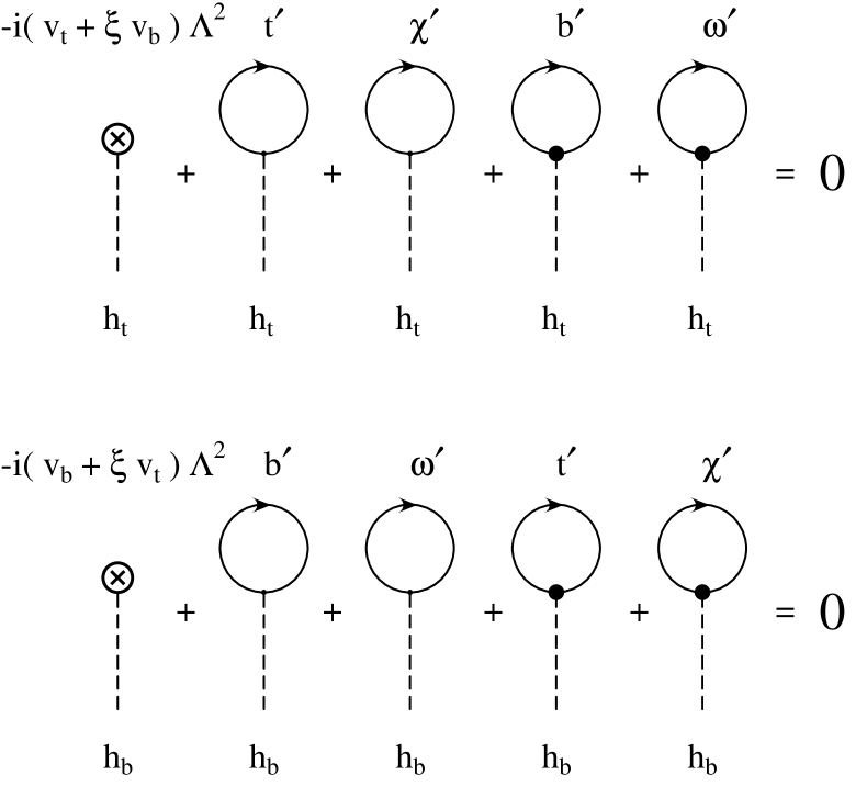
Figure 13: Coupled gap equations for top and bottom seesaws up to ${\cal O}(\xi)$. The black dots denote the vertices associated with small $\xi$ couplings.

Now, we are ready to solve the gap equations for the top-bottom seesaw system. We note that our extended model has three input parameters $\left(\Lambda,\,\kappa/\kappa_{c},\,\tan\beta\right)$, and three extra unknown parameters $(m_{b\omega},\,r_{b},\,\mu_{\omega\omega})$ (with $r_{b}\equiv\mu_{\omega b}/\mu_{\omega\omega}$) from the $b$-seesaw sector, in addition to $(m_{t\chi},\,r_{t},\,\mu_{\chi\chi})$ from the $t$-seesaw sector. On the other hand, we have six physical conditions in total: two seesaw gap equations [in Eq. (98)], two Pagels-Stokar formulae [in Eq. (102)], and two mass-eigenvalue equations [in Eq. (2.1) for $m_{t}$ and a similar one for $m_{b}$]. Thus, all six seesaw parameters can be completely solved as functions of $\Lambda$ for each given $\left(\kappa/\kappa_{c},\,\tan\beta\right)$. Consequently, the masses of ${\chi}$ and ${\omega}$ are also predicted, together with all seesaw mixing angles. We display our systematic numerical solutions for a wide range of $\tan\beta$ values in Fig. 14, where we have chosen $\xi\lesssim 10^{-3}$ and found that the $\xi$-corrections are negligible and the difference from $\xi=0$ case is invisible in the plots. From this figure, we also see that the $\chi$ and $\omega$ are highly degenerate for all solutions; the same feature holds for the parameters $(\mu_{\chi\chi},\,\mu_{\omega\omega})$ when $\Lambda\gtrsim 2-3$ TeV. This fact can be understood by noting that the real difference between the top and bottom sectors is controlled by the experimental ratio $m_{t}/m_{b}\approx 40\gg 1$ and the input ratio $\tan\beta=v_{t}/v_{b}$. The former is connected to seesaw parameters via,

$$\frac{m_{t}}{m_{b}}\approx\frac{m_{t\chi}\mu_{\chi t}/\mu_{\chi\chi}}{m_{b\omega}\mu_{\omega b}/\mu_{\omega\omega}}=\frac{m_{t\chi}}{m_{b\omega}}\sqrt{\frac{r_{t}}{r_{b}}}\,,$$ (103)

while the latter can be deduced from the Pagels-Stokar formula (102) after ignoring the ${\cal O}(\xi)$ corrections and the insensitive logarithmic factors, i.e., $\tan\beta=v_{t}/v_{b}\sim m_{t\chi}/m_{b\omega}$, where we have also expanded the right-hand sides of (102) like Eq. (33) in which we can see the heavy masses $(M_{\chi},\,M_{\omega})$ [or $(\mu_{\chi\chi},\,\mu_{\omega\omega})$] of the vector-like fermions $({\chi},\,w)$ have only logarithmic dependence, obeying the decoupling theorem [32, 33]. Similar decoupling behavior appears on the right-hand sides of the gap equations (98)-(100). Indeed, it is this decoupling nature that makes the right-hand side of (102) insensitive to $(M_{\chi},\,M_{\omega})$. Thus, we arrive at two approximate relations below, which control the qualitative features of the two sectors,

$$\sqrt{\frac{r_{t}}{r_{b}}}\sim\frac{m_{t}/m_{b}}{\tan\beta}\sim\frac{40}{\tan\beta}\,,~{}~{}~{}~{}~{}~{}\frac{m_{t\chi}}{m_{b\omega}}\sim\tan\beta\,.$$ (104)

Using these, we can now understand, in Fig. 14, why the main difference between $t$ and $b$ sectors are reflected in the ratios $(r_{t},\,r_{b})$ for small $\tan\beta$ values, but manifest in the mass-gaps $(m_{t\chi},\,m_{b\omega})$ for large $\tan\beta$ values. Finally, because of their vector-like decoupling nature, the heavy masses $(M_{\chi},\,M_{\omega})$ or $(\mu_{\chi\chi},\,\mu_{\omega\omega})$ remain highly degenerate, and numerically they are located at around $(0.63-0.65)\Lambda$ for $\kappa/\kappa_{c}=2$, as shown in Fig. 14. However, we expect such a picture for the $b$-sector to be modified when $\xi$-correction to the mass gap $m_{b\omega}$ becomes significant in the very high $\tan\beta$ region. As a typical case, we may consider $\tan\beta=40$ and $\xi=2\times 10^{-2}$ [which is a generic size of the Topcolor instanton contribution with $c_{0}={\cal O}(1)$ and $\kappa/\kappa_{c}=2$ in Eq. (88)]. In this case, we deduce a ratio $(\xi v_{t})/v_{b}=\xi\tan\beta=80\%$ for the mass-gap $m_{b\omega}$ in Eq. (97), implying that the $\xi$-term makes up about $80\%$ of $m_{b\omega}$ and the $b$ mass. Consequently, the Eq. (102) no longer gives the relation $v_{t}/v_{b}\sim m_{t\chi}/m_{b\omega}$ [and thus (104)] because in the second formula of Eq. (102) the $\xi m_{t\chi}$ term is non-negligible on the right-hand side. But, the $t$-sector remains essentially the same as before since in the mass-gap $m_{t\chi}$ [cf. Eq. (97)] the ratio $(\xi v_{b})/v_{t}=\xi/\tan\beta\lll 1$ and is completely negligible even for small $\tan\beta$. Our numerical solutions for this large $(\tan\beta,\,\xi)$ scheme are shown as dashed curves in Fig. 15, in comparison with the small or zero $\xi$ cases ($\xi\lesssim 10^{-3}$) shown as dotted curves. Indeed, we see sizable modifications for the seesaw parameters in the $b$-sector, i.e., the gap $m_{b\omega}$ is lifted up by a factor of $\sim\!2$ while the ratio $r_{b}=\mu_{\omega b}/\mu_{\omega\omega}$ is shifted down by about one-half. As a consequence, the mass scale $M_{\omega}$ (or $\mu_{\omega\omega}$) for ${\omega}$ is also pushed up somewhat, closer to the scale $\Lambda$. This gives an interesting example in which the effects of Topcolor instantons [7] are significant and provide the dominant contribution to the bottom mass.

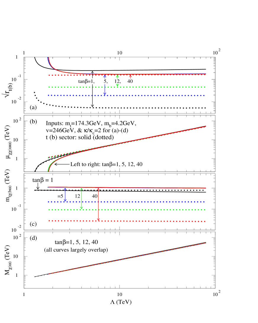
Figure 14: Solutions of the top and bottom seesaw gap equations with $\kappa/\kappa_{c}=2$ and $\tan\beta\in(1,\,5,\,12,\,40)$, where we have superimposed the physical constraints, $(m_{t},\,m_{b})=(174.3,\,4.2)$ GeV and $v=246$ GeV. The solid curves are for the top sector while the dotted curves for the bottom sector. Here we have chosen the region $\xi\lesssim 10^{-3}$ in which the $\xi$-effects are negligible (invisible).

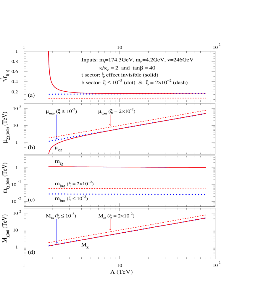
Figure 15: The effect of the ${\cal O}(\xi)$ corrections on the physical seesaw solutions, for $\kappa/\kappa_{c}=2$ and $\tan\beta=40$. The solid curves are for the top sector while the bottom sector is depicted by dotted curves [$\xi\lesssim{\cal O}(10^{-3})$] and dashed curves [$\xi=2\times 10^{-2}$]. A sizable value of $\xi=2\times 10^{-2}$ (representing typical instanton effect) can provide about $80\%$ of the $b$ mass for $\tan\beta=40$; while for $\xi\lesssim{\cal O}(10^{-3})$, the $b$ mass is almost fully given by ${\cal O}(\xi^{0})$ seesaw corrections.

3.3 Mass Spectrum of Composite Higgs Sector

We proceed to analyze the physical Higgs mass spectrum of this extended model. Starting from the Lagrangian ${\cal L}_{\rm mass}+{\cal L}_{\rm int}+{\cal L}_{\rm PQB}$  at $\mu=\Lambda$ and performing the seesaw mass diagonalization, we evolve it down to the scale $\mu\left(<M_{{\chi},{\omega}}\leq\Lambda\right)$ by integrating out the loop momenta between $\mu$ and $\Lambda$ and arrive at the renormalized effective Lagrangian with only light quarks $(t^{\prime},\,b^{\prime})$ and the two-doublet Higgs bosons,

$$\begin{array}[]{l}{\cal L}_{\mu<M_{{\chi},{\omega}}\leq\Lambda}\,=\,\displaystyle-m_{t}\;\overline{t^{\prime}}t^{\prime}-m_{b}\;\overline{b^{\prime}}b^{\prime}\\[8.53581pt] \hskip 14.22636pt\displaystyle-\frac{1}{\sqrt{2}}\left[g_{t}c_{L}^{t}s_{R}^{t}\;\overline{t^{\prime}}t^{\prime}h_{t}^{0}+g_{b}c_{L}^{b}s_{R}^{b}\;\overline{b^{\prime}}b^{\prime}h_{b}^{0}\right]-\frac{i}{\sqrt{2}}\left[g_{t}c_{\beta}c_{L}^{t}s_{R}^{t}\;\overline{t^{\prime}}\gamma_{5}t^{\prime}h_{t}^{0}+g_{b}s_{\beta}c_{L}^{b}s_{R}^{b}\;\overline{b^{\prime}}\gamma_{5}b^{\prime}h_{b}^{0}\right]A^{0}\\[11.38109pt] \hskip 14.22636pt\displaystyle-\;\overline{b^{\prime}}\left[g_{t}c_{\beta}c_{L}^{b}s_{R}^{t}P_{R}+g_{b}s_{\beta}s_{R}^{b}c_{L}^{t}P_{L}\right]t^{\prime}H^{-}+{\rm h.c.}-\left[\Delta\widetilde{T}_{t}\;h_{t}^{0}+\Delta\widetilde{T}_{b}\;h_{b}^{0}\right]\\[11.38109pt] \hskip 14.22636pt\displaystyle-\displaystyle\frac{1}{2}\left[M_{22}^{2}{h_{t}^{0}}^{2}+M_{11}^{2}{h_{b}^{0}}^{2}+2\xi M_{12}^{2}h_{t}^{0}h_{b}^{0}+M_{A}^{2}{A^{0}}^{2}+2M_{H^{\pm}}^{2}H^{+}H^{-}\right]-V_{\rm int}(h_{t}^{0},h_{b}^{0},A^{0},H^{\pm})\,,\end{array}$$ (105)

where $(g_{t},\,g_{b})=(h_{1}/{Z_{h_{t}}^{1/2}},\,h_{1}/{Z_{h_{b}}^{1/2}})$, $(s_{\beta},\,c_{\beta})=(\sin\!\beta,\,\cos\!\beta)$, $P_{L,R}=(1\mp\gamma_{5})/2$, and the unitary gauge is chosen so that only the physical Higgs scalars $(h_{t}^{0},h_{b}^{0},A^{0},H^{\pm})$ are relevant. Here, $\Delta\widetilde{T}_{t}$ and $\Delta\widetilde{T}_{b}$ are the tadpole terms which we used to derive the gap equations (98) above. The Higgs mass terms are computed up to ${\cal O}(\xi)$ and are expressed as,

$$\begin{array}[]{lll}M_{22}^{2}=M_{22,0}^{2}+\xi\delta M_{22}^{2}\,,{}{}&M_{11}^{2}=M_{11,0}^{2}+\xi\delta M_{11}^{2}\,,{}{}&\xi M_{12}^{2}=\xi\delta M_{12}^{2}\,,\\[11.38109pt] M_{H^{\pm}}^{2}=M_{\pm,0}^{2}+\xi\delta M_{\pm}^{2}\,,{}{}&M_{A}^{2}=\xi\delta M_{A}^{2}\,,&\end{array}$$ (106)

where the leading $O(\xi^{0})$ contributions are,

$$\begin{array}[]{l}\displaystyle M_{22,0}^{2}\!=M_{h}^{2}[{\rm Eq.}(\ref{eq:Mh})]\left|{}_{(s,c)_{L,R}\rightarrow(s^{t},c^{t})_{L,R}}\,,~{}~{}\right.M_{11,0}^{2}\!=M_{h}^{2}[{\rm Eq.}(\ref{eq:Mh})]\left|{}_{(s,c)_{L,R}\rightarrow(s^{t},c^{t})_{L,R}}^{(m_{t},M_{\chi})\rightarrow(m_{b},M_{\omega})}\,,~{}~{}\right.\\[14.22636pt] \displaystyle M_{\pm,0}^{2}\;\!=\displaystyle\frac{\kappa}{\kappa_{c}}\left[\Lambda^{2}\left(Z_{h_{t}}^{-1}c_{\beta}^{2}+Z_{h_{b}}^{-1}s_{\beta}^{2}\right)\left(\frac{\kappa_{c}}{\kappa}-1\right)+\left(a_{11}m_{t}^{2}+a_{12}\right)\ln\left(\frac{\Lambda^{2}}{m_{t}^{2}}+1\right)\right.\\[17.07164pt] \hskip 65.44133pt\displaystyle\left.+\left(\overline{a}_{21}M_{\chi}^{2}+a_{22}\right)\ln\left(\frac{\Lambda^{2}}{M_{\chi}^{2}}+1\right)+\left(\overline{a}_{31}M_{\chi}^{2}+a_{32}\right)\ln\left(\frac{\Lambda^{2}}{M_{\omega}^{2}}+1\right)\right],\\[17.07164pt] \left(\!\!\begin{array}[]{l}a_{11}\\[5.69054pt] a_{21}\\[5.69054pt] a_{31}\\[5.69054pt] a_{41}\end{array}\!\!\right)\!=\!\displaystyle\frac{c_{\beta}^{2}}{Z_{h_{t}}}\!\left(\!\!\begin{array}[]{l}(s_{R}^{t}c_{L}^{b})^{2}\\[5.69054pt] (c_{R}^{t}c_{L}^{b})^{2}\\[5.69054pt] (s_{R}^{t}s_{L}^{b})^{2}\\[5.69054pt] (c_{R}^{t}c_{L}^{b})^{2}\end{array}\!\!\right)\!\!+\!\frac{s_{\beta}^{2}}{Z_{h_{b}}}\!\left(\!\!\begin{array}[]{l}(c_{L}^{t}s_{R}^{b})^{2}\\[5.69054pt] (s_{L}^{t}s_{R}^{b})^{2}\\[5.69054pt] (c_{L}^{t}c_{R}^{b})^{2}\\[5.69054pt] (s_{L}^{t}c_{R}^{b})^{2}\end{array}\!\!\right)\!,~{}~{}~{}\left(\!\!\begin{array}[]{l}a_{12}\\[5.69054pt] a_{22}\\[5.69054pt] a_{32}\\[5.69054pt] a_{42}\end{array}\!\!\right)\!=\!\frac{2s_{\beta}c_{\beta}}{{Z_{h_{t}}^{\frac{1}{2}}Z_{h_{b}}^{\frac{1}{2}}}}\!\!\left(\!\!\begin{array}[]{l}m_{t}m_{b}c_{L}^{t}s_{R}^{t}c_{L}^{b}s_{R}^{b}\\[5.69054pt] M_{\chi}m_{b}s_{L}^{t}c_{R}^{t}c_{L}^{b}s_{R}^{b}\\[5.69054pt] M_{\omega}m_{t}s_{L}^{t}c_{R}^{t}c_{L}^{b}s_{R}^{b}\\[5.69054pt] M_{\chi}M_{\omega}s_{L}^{t}c_{R}^{t}s_{L}^{b}c_{R}^{b}\end{array}\!\!\right)\!,\end{array}$$ (107)

with $\,\overline{a}_{21}=a_{21}+(a_{41}M_{\chi}^{2}+a_{42})/(M_{\chi}^{2}-M_{\omega}^{2}),\,$ and $\,\overline{a}_{31}=a_{31}+(a_{41}M_{\omega}^{2}+a_{42})/(M_{\omega}^{2}-M_{\chi}^{2}).\,$ The axionic pseudo-scalar $A^{0}$ is massless at this order due to the Peccei-Quinn symmetry (85). One recovers a simple and intuitive picture under the approximate limit $(r_{t},\,r_{b})\ll 1$, i.e.,

$$M_{22,0}\approx 2m_{t\chi}\,,~{}~{}~{}M_{11,0}\approx 2m_{b\omega}\,,~{}~{}~{}M_{\pm,0}\approx\sqrt{2}\left(m_{t\chi}^{2}+m_{b\omega}^{2}\right)^{\frac{1}{2}}\,,$$ (108)

which are all controlled by the dynamical mass gaps $(m_{t\chi},\,m_{b\omega})$ and become equal in the special case of $\tan\beta=1$, as expected. These approximate formulae agree with our independent Higgs potential analysis in Appendix-B.

For the ${\cal O}(\xi)$ corrections, we first perform a careful calculation of the $A^{0}$ mass, and obtain,

$$M^{2}_{A}\! = \!\xi\delta M_{A}^{2}\,=\,\frac{2\xi\Lambda^{2}}{\displaystyle\sin\!2\beta\sqrt{Z_{h_{t}}Z_{h_{b}}}}\,+\,{\cal O}(\xi^{2})\,.$$ (109)

It is remarkable to notice that the Peccei-Quinn breaking mass $M_{A}$ is proportional to $\sqrt{\xi}\Lambda$ instead of being controlled by the dynamical mass gaps $(m_{t\chi},\,m_{b\omega})$. As noted above, the essential difference between $A^{0}$ and the other Higgs scalars is that $A^{0}$ is a massless Goldstone boson at ${\cal O}(\xi^{0})$ and its non-vanishing mass comes from the explicit Peccei-Quinn breaking $\xi$-term. Hence, it is natural to see that $M_{A}$ is not controlled by the dynamical gaps $(m_{t\chi},\,m_{b\omega})$, but instead scales like  $\sqrt{\xi}\Lambda$ . This results in the $A^{0}$ being relatively heavier than naively expected, provided $\xi\gtrsim 10^{-3}$. Such an ${\cal O}(\xi\Lambda^{2})$ correction also shows up in other Higgs mass formulae at ${\cal O}(\xi)$ and is thus a generic feature of the explicit Peccei-Quinn breaking. So, we can express the leading $\xi$-corrections to $(h_{t}^{0},\,h_{b}^{0},\,H^{\pm})$ masses in terms of $M_{A}^{2}$ while the rest of the $\xi$-terms are of ${\cal O}(\xi m_{t\chi}^{2},\,\xi m_{b\omega}^{2})$ and thus much less significant. With this in mind, we compactly summarize the ${\cal O}(\xi)$ masses of $(h_{t}^{0},\,h_{b}^{0},\,H^{\pm})$ as,

$$\begin{array}[]{l}\xi\delta M_{11}^{2}\simeq s_{\beta}^{2}M_{A}^{2}\,,~{}~{}~{}~{}\xi\delta M_{22}^{2}\simeq c_{\beta}^{2}M_{A}^{2}\,,~{}~{}~{}~{}\xi\delta M_{12}^{2}\simeq-s_{\beta}c_{\beta}M_{A}^{2}+4\xi\left(m_{t\chi}^{2}+m_{b\omega}^{2}\right)\,,\\[8.53581pt] \xi\delta M_{\pm}^{2}\simeq M_{A}^{2}-\xi\left(\cot\!\beta\;m_{t\chi}^{2}+\tan\beta\;m_{b\omega}^{2}\right)\,,\end{array}$$ (110)

which can be most easily extracted from the Higgs potential analysis shown in Appendix-B. Due to the mixing mass term between $h_{t}^{0}$ and $h_{b}^{0}$, we diagonalize them into the mass-eigenstates $(h^{0},\,H^{0})$ with the physical masses,

$$M_{h,H}^{2}=\displaystyle\frac{1}{2}\left[M_{11}^{2}+M_{22}^{2}\pm\sqrt{\left(M_{11}^{2}-M_{22}^{2}\right)^{2}+4M_{12}^{4}}\;\right]\,.$$ (111)

The corresponding rotation angle $\alpha\in[-\pi/2,\,0]$ is determined by $\tan(2\alpha)=2M_{12}^{2}/(M_{11}^{2}-M_{22}^{2})$.

Based upon these, we can finally analyze the Higgs mass spectrum of this model using the physical solutions to the seesaw gap equations derived in the previous subsection. We present our numerical results in Fig. 16, where we choose $\kappa/\kappa_{c}=2$ and a wide range of $\tan\beta$ values. The Peccei-Quinn breaking parameter $\xi$ is set to a representative value of $\xi=3\times 10^{-3}$ for all plots. The proportionality of $M_{A}$ with $\Lambda$ can be clearly seen, and as $M_{A}$ moves above $1$ TeV, the Higgs bosons $(H^{0},\,H^{\pm})$ becomes much more degenerate with $A^{0}$, while the lightest neutral Higgs $h^{0}$ remains around $1$ TeV, saturating the SM unitarity bound. This is a quite generic feature of this model unless the parameter $\xi$ is much smaller, around $10^{-4}$ or below, which is unlikely in the Topcolor instanton picture. Also, too small $\xi~{}(\lesssim 10^{-4}-10^{-5})$ will have more significant mass-splittings among Higgs bosons $(A^{0},\,H^{0},\,H^{\pm})$ which cause large weak-isospin violation in the oblique parameter $T$ (besides resulting in a very light axion $A^{0}$). This is disfavored from the experimental viewpoint. Thus, our analysis favors a relatively heavy axion $A^{0}$ (together with other Higgs scalars) and the Topcolor instanton [7] interpretation of the Peccei-Quinn breaking for this model.

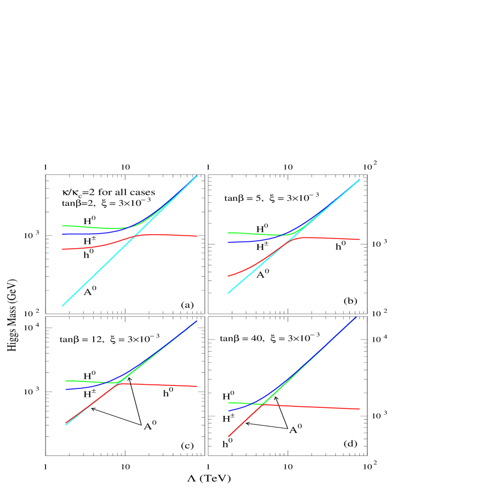
Figure 16: The mass spectrum of the Higgs bosons are plotted for $\kappa/\kappa_{c}=2$ and $\tan\beta\in(2,\,5,\,12,\,40)$ in the extended model with bottom seesaw, where the parameter $\xi$ is representatively chosen as $\xi=3\times 10^{-3}$

4 Constraints from Precision Observables

After quantitative analyses on the vacuum structure and composite Higgs spectrum in the dynamical Top Seesaw models, we proceed to systematically study their experimental constraints from the electroweak precision data. The most important bounds come from the radiative corrections to the oblique parameters $T$ and $S$ [19] and also the corrections to the ${Zb\bar{b}}$ vertex induced by the $b$-$\omega$ mixing in the bottom seesaw sector. It is remarkable that the minimal Top Seesaw model, having a typical heavy composite Higgs boson around $1$ TeV, is non-trivially compatible with the $S-T$ bounds, due to the conspiracy from the large positive seesaw correction to the $T$ parameter. The case for the extended model with bottom seesaw is more complex because of the $b$-${\omega}$ mixing and the two Higgs doublets. In this extended model the precision $T$ bound requires a certain degeneracy in the mass spectrum of the Higgs scalars and thus favors a relatively heavy axion $A^{0}$. As we will show, with the Topcolor instanton interpretation of the Peccei-Quinn breaking, the resulting precision bounds on the heavy ${\chi}$ and ${\omega}$ masses are at the similar level to that of the minimal Top seesaw model.

4.1 In the Minimal Top Seesaw Model

The minimal Top seesaw model has a single composite Higgs boson in addition to the singlet seesaw quark ${\chi}$ in the spectrum. As we have shown in Fig. 12, this composite Higgs scalar has its mass typically around $\sim\!1$ TeV. Its contributions to the oblique $S$ and $T$ parameters can be expressed as,

$$\begin{array}[]{lll}\Delta S_{H}&=&\displaystyle+\frac{1}{12\pi}\ln\left(\frac{M^{2}_{h}}{m_{h,{\rm ref}}^{2}}\right),\\[14.22636pt] \Delta T_{H}&=&\displaystyle-\frac{3}{16\pi\cos^{2}\theta_{W}}\ln\left(\frac{M^{2}_{h}}{m_{h,{\rm ref}}^{2}}\right),\end{array}$$

where $m_{h,{\rm ref}}$ is the reference point of the SM Higgs mass. Since in the pure SM the current precision data [34] favors a light Higgs mass around $100$ GeV, we see that a heavy Higgs scalar with a $\sim\!1$ TeV mass will drive $\Delta T$ in the negative direction relative to a light SM Higgs and thus is excluded by the current precision $S-T$ contour shown in Fig. 17(a). However, the top seesaw sector has generic weak-isospin violation from the $t$-$\chi$ mixing which will significantly contribute to $\Delta T$ in the positive direction, as can be seen from the formula,

$$\Delta T = \frac{N_{c}}{16\pi^{2}v^{2}\alpha}\left[s_{L}^{4}M^{2}_{\chi}-s_{L}^{2}(1+c_{L}^{2})m_{t}^{2}+2s_{L}^{2}c_{L}^{2}\frac{M_{\chi}^{2}m_{t}^{2}}{M_{\chi}^{2}-m_{t}^{2}}\ln\frac{M_{\chi}^{2}}{m_{t}^{2}}\right]$$ (112)

$$= \frac{N_{c}m_{t}^{2}}{16\pi^{2}v^{2}\alpha}\left[2\left(\ln\frac{M_{\chi}^{2}}{m_{t}^{2}}-1\right)+\frac{1}{r_{t}}\right]\frac{(m_{t}/\mu_{\chi t})^{2}}{1+r_{t}}+{\cal O}\left(\frac{m_{t}^{4}}{\mu_{\chi t}^{4}}\right)\,,$$

in which $r_{t}=(\mu_{\chi t}/\mu_{\chi\chi})^{2}\lesssim 1$. Here, we have subtracted out the usual SM top contribution as it was already included in the precision fit. The expanded formula indeed shows a sizable $\Delta T>0$; it also exhibits the decoupling nature of the vector-like heavy quark ${\chi}$, since the large mass parameters go with negative powers (for fixed ratio $r_{t}$).

Next, we compute the $\chi-t$ contribution to $\Delta S$, and obtain,

$$\Delta S = \frac{N_{c}}{36\pi}s_{L}^{2}\left\{44\left(\frac{M_{\chi}^{2}}{m_{z}^{2}}-\frac{m_{t}^{2}}{m_{z}^{2}}\right)-2\ln\frac{M_{\chi}^{2}}{m_{t}^{2}}-18c_{L}^{2}G_{1}\!\left(\frac{m_{t}^{2}}{m_{z}^{2}},\frac{M^{2}_{\chi}}{m_{z}^{2}}\right)\right.$$ (113)

$$\hskip 44.10176pt\left.-\left(11\frac{m_{t}^{2}}{m_{z}^{2}}+1\right)F_{1}\!\left(\frac{m^{2}_{t}}{m_{z}^{2}}\right)+\left(11\frac{M_{\chi}^{2}}{m_{z}^{2}}+1\right)F_{1}\!\left(\frac{M^{2}_{\chi}}{m_{z}^{2}}\right)\right\}$$

$$= \frac{N_{c}}{9\pi}\left[\displaystyle\ln\frac{M_{\chi}^{2}}{m_{t}^{2}}-\frac{5}{2}+\frac{m_{z}^{2}}{20m_{t}^{2}}\right]\frac{(m_{t}/\mu_{\chi t})^{2}}{1+r_{t}}+{\cal O}\left(\frac{m_{t}^{4}}{\mu_{\chi t}^{4}}\right)\,,$$

where $m_{z}$ is the mass of weak gauge boson $Z^{0}$, and the relevant functions $F_{1}(y)$ and $G_{1}(y_{1},y_{2})$ are defined as,

$$F_{1}(y) = -4\sqrt{4y-1}\>{\rm arctan}\frac{1}{\sqrt{4y-1}}\,,$$ (114)

$$G_{1}(y_{1},y_{2}) = \frac{5(y_{1}^{2}+y_{2}^{2})-2y_{1}y_{2}}{9(y_{1}-y_{2})^{2}}+\frac{3y_{1}y_{2}(y_{1}+y_{2})-y_{1}^{3}-y_{2}^{3}}{3(y_{1}-y_{2})^{3}}\ln\frac{y_{1}}{y_{2}}\,.$$ (115)

Now, Keeping the dominant leading logarithmic terms in the above expanded formulae, we can directly estimate the relative size of $\Delta S$ versus $\Delta T$,

$$\frac{\Delta S}{\Delta T}\approx\frac{16\pi\alpha}{9}\approx 0.04\ll 1\,,$$ (116)

which shows that $\Delta S$ is only about $4\%$ of $\Delta T$ and thus negligible in comparison with the typical values of $\Delta T>0$, as advertised earlier in the introduction.

In Fig. 17, we assemble the complete $\Delta S$ and $\Delta T$ contributions from the minimal top seesaw model, including both the corrections from the composite Higgs boson and the seesaw quarks, and compare them with the 95% C.L. contour for $\Delta S-\Delta T$. Each figure corresponds to a different choice of $\kappa/\kappa_{c}$, and shows the trajectory in the $\Delta S-\Delta T$ plane as the $\chi$ mass varies. As a comparison, we have plotted the results based on both the large-$N_{c}$ fermion-bubble calculation and the improved RG approach (cf. Sec. 2.6). For the relevant parameter space here, the improved RG approach gives lower Higgs mass values (around $400-500$ GeV) so that the curves are slightly shifted towards the upper left. As a consequence, in the improved RG approach the upper bound on $M_{\chi}$ is more relaxed for $\kappa/\kappa_{c}\gtrsim 1.2$, while the lower bound on $M_{\chi}$ remains at a similar level. The figure clearly illustrates that the top seesaw model can be consistent with the electroweak precision data provided $M_{\chi}$ is in the appropriate mass range. For instance, when the Topcolor force is slightly super-critical, we see that precision data are effectively probing $M_{\chi}\sim 4$ TeV. A high luminosity Linear Collider at GigaZ can further improve these indirect precision constraints on the Top seesaw dynamics with a much smaller $\Delta S-\Delta T$ error ellipse [27]. Finally, in Fig. 18, we display the same $\Delta S-\Delta T$ trajectories as in Fig. 17, but with the corresponding Higgs mass ($M_{h}$) values marked. We see that as each trajectory moves up along the $\Delta T$ direction, the $M_{h}$ value changes very little and thus the rise of $\Delta T$ is really due to the decrease of $M_{\chi}$ (as marked in Fig. 17). The Fig. 18 further shows that the relevant Higgs mass is about $1-1.4$ TeV in the large-$N_{c}$ fermion-bubble calculation and $400-500$ GeV in the improved RG approach. As we explained in Sec. 2.6, the large-$N_{c}$ fermion-bubble calculation may over-estimate $M_{h}$ due to the ignorance of non-large-$N_{c}$ effects of the Higgs propogation in the loop, while the improved RG approach may under-estimate $M_{h}$ due to the sizable uncertainties associated with the compositeness condition at the scale $\Lambda\sim 10^{4-5}$ GeV and the use of simple mass-independent renormalization in such low cutoff theories. So, the two approaches are complementary and the real $M_{h}$ values should lie between these two estimates. Actually, the shift between the two trajectories along the $\Delta S$ direction is mainly due to the effect of the Higgs mass. Thus, taking into account our ignorance of the detailed dynamics around the scale $\Lambda$ and above, we may view the region between the two trajectories inside the $\Delta S-\Delta T$ ellips as the viable parameter space allowed by the precision data.

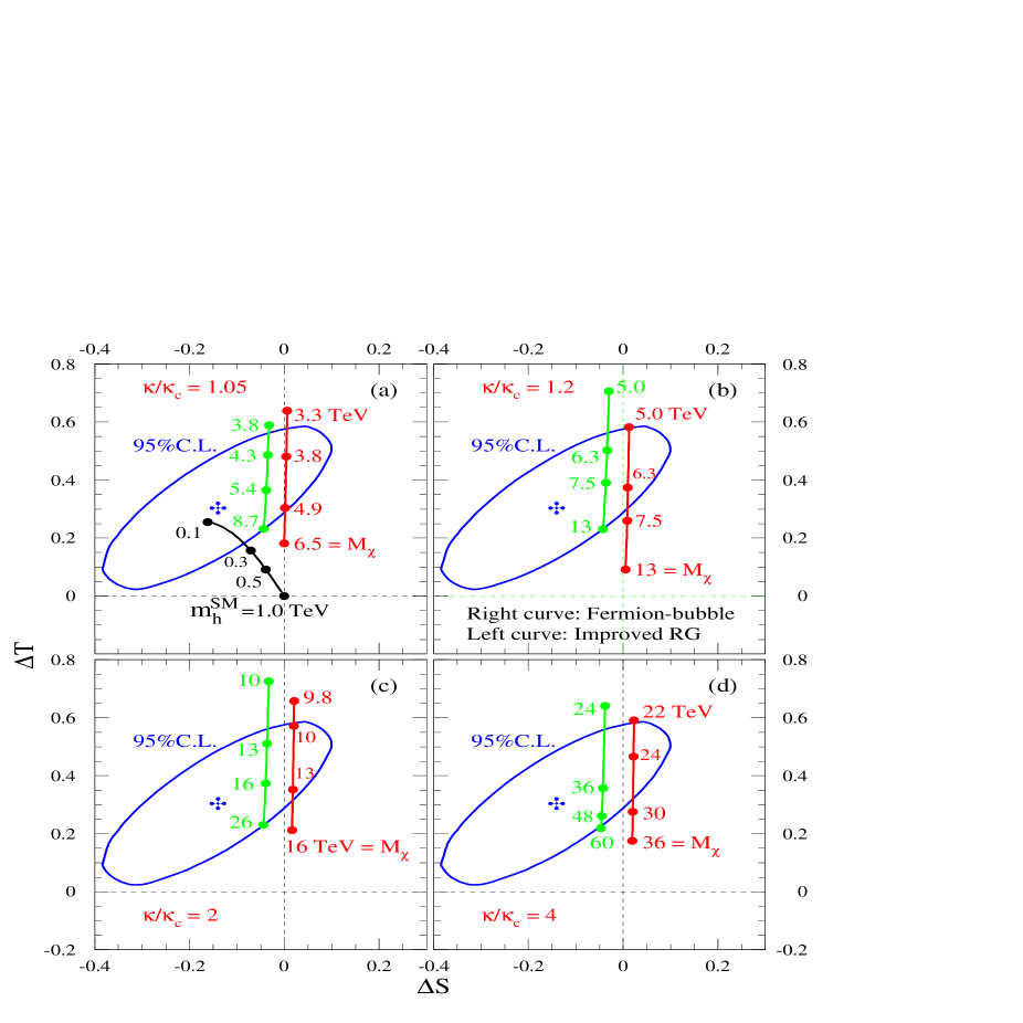
Figure 17: Top seesaw contributions to $\Delta S$ and $\Delta T$ are compared with the 95% C.L. error ellipse (with $m_{h}^{\rm ref}=1$ TeV) for $\kappa/\kappa_{c}=1.05,\,1.2,\,2,\,4$. The $\Delta S$-$\Delta T$ trajectories (including both Higgs and $\chi$ contributions) are shown as a function of $M_{\chi}$. In each plot, the curve on the right is derived from the large-$N_{c}$ fermion bubble calculation, and as a comparison, the curve on the left is deduced by an improved RG approach (cf. Sec. 2.6). For reference, the SM Higgs corrections to ($S$, $T$), relative to $m_{h}^{\rm ref}=1$ TeV, are given for $m_{h}^{\rm SM}$ varying from 100 GeV up to 1.0 TeV in plot (a).

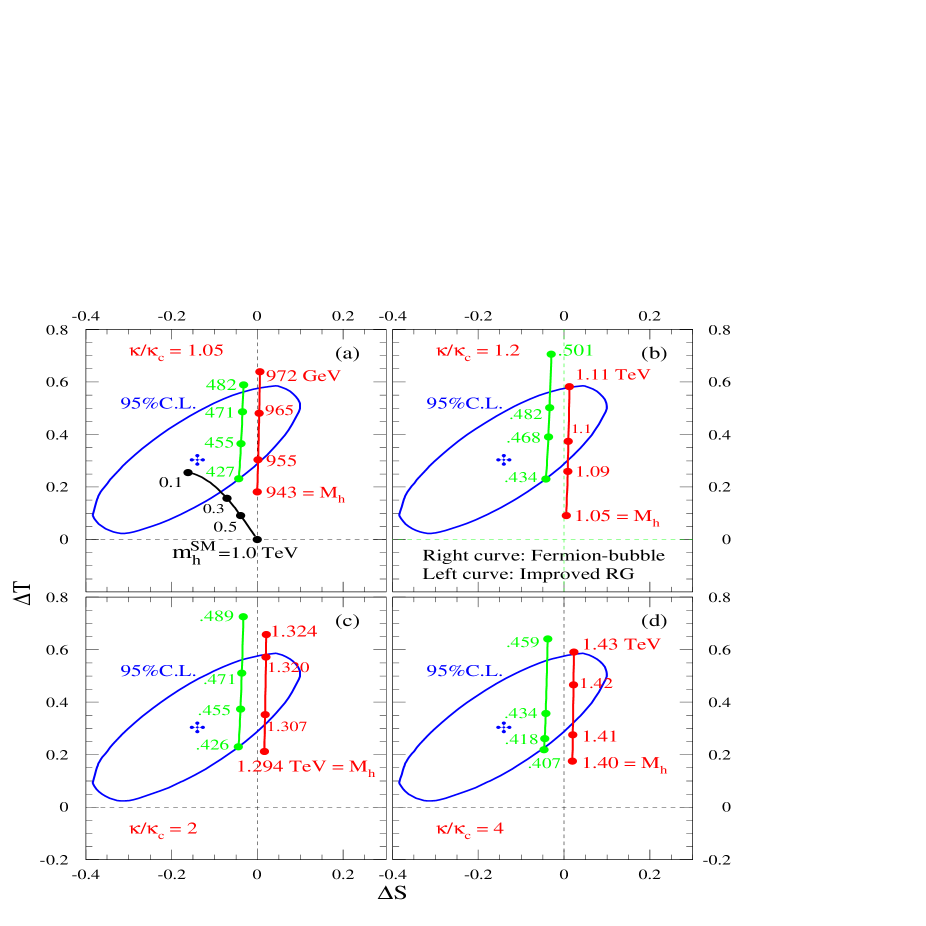
Figure 18: Same as Fig. 17, but with the corresponding $M_{h}$ values marked on the $\Delta S$-$\Delta T$ trajectories instead. It shows that each trajectory is very insensitive to $M_{h}$ and the large increase along the positive $\Delta T$ direction is due to the top seesaw contribution as $M_{\chi}$ decreases (cf. Fig. 17). In each plot, the shift of the left trajectory relative to the right one is due to the smaller $M_{h}$ values (estimated around $400-500$ GeV), but $\Delta S\ll\Delta T$ generally holds so that $\Delta S$ is much less significant.

4.2 In the Extended Model with Bottom Seesaw

The inclusion of a bottom seesaw generates additional $b$-${\omega}$ mixing which have nontrivial contributions to the $S$ and $T$ parameters and also to the ${Zb\bar{b}}$ vertex. Furthermore, the composite Higgs sector now contains two doublets and thus has additional corrections to the precision observables. We start by calculating the complete set of loop diagrams [including the mass-eigenstate seesaw quarks $(t^{\prime},\,b^{\prime},\,{\chi}^{\prime},\,{\omega}^{\prime})$] that contribute to the $S$ and $T$ parameters. The general results can be summarized below,

$$\begin{array}[]{lll}\Delta S&=&\displaystyle\frac{N_{c}}{36\pi}\left\{s^{t\,2}_{L}\left[44\left(\frac{M_{\chi}^{2}}{m_{z}^{2}}-\frac{m_{t}^{2}}{m_{z}^{2}}\right)-2\ln\frac{M_{\chi}^{2}}{m_{t}^{2}}-18c_{L}^{t\,2}G_{1}\!\left(\frac{m_{t}^{2}}{m_{z}^{2}},\frac{M^{2}_{\chi}}{m_{z}^{2}}\right)\right.\right.\\[17.07164pt] &&\hskip 65.44133pt\displaystyle\left.-\left(11\frac{m_{t}^{2}}{m_{z}^{2}}+1\right)F_{1}\!\left(\frac{m^{2}_{t}}{m_{z}^{2}}\right)+\left(11\frac{M_{\chi}^{2}}{m_{z}^{2}}+1\right)F_{1}\!\left(\frac{M^{2}_{\chi}}{m_{z}^{2}}\right)\right]\\[17.07164pt] &&\hskip 24.18483pt\displaystyle+s^{b\,2}_{L}\left[28\left(\frac{M_{\omega}^{2}}{m_{z}^{2}}-\frac{m_{b}^{2}}{m_{z}^{2}}\right)+2\ln\frac{M_{\omega}^{2}}{m_{b}^{2}}-18c_{L}^{b\,2}G_{1}\!\left(\frac{m_{b}^{2}}{m_{z}^{2}},\frac{M^{2}_{\omega}}{m_{z}^{2}}\right)\right.\\[17.07164pt] &&\left.\left.\hskip 65.44133pt\displaystyle-\left(7\frac{m_{b}^{2}}{m_{z}^{2}}-1\right)F_{2}\!\left(\frac{m^{2}_{b}}{m_{z}^{2}}\right)+\left(7\frac{M_{\omega}^{2}}{m_{z}^{2}}-1\right)F_{1}\!\left(\frac{M^{2}_{\omega}}{m_{z}^{2}}\right)\right]\right\},\end{array}$$ (117)

$$\begin{array}[]{lll}\Delta T&=&\displaystyle\frac{N_{c}}{16\pi s^{2}_{w}c^{2}_{w}m_{z}^{2}}\left[s^{t\,2}_{L}c^{b\,2}_{L}F_{3}\!\left(M^{2}_{\chi},m^{2}_{b}\right)+c^{t\,2}_{L}s^{b\,2}_{L}F_{3}\!\left(M^{2}_{\omega},m^{2}_{t}\right)+s^{t\,2}_{L}s^{b\,2}_{L}F_{3}\!\left(M^{2}_{\chi},M^{2}_{\omega}\right)\right.\\[14.22636pt] &&\left.\hskip 56.9055pt-s^{t\,2}_{L}c^{t\,2}_{L}F_{3}\!\left(M^{2}_{\chi},m^{2}_{t}\right)-s^{b\,2}_{L}c^{b\,2}_{L}F_{3}\!\left(M^{2}_{\omega},m^{2}_{b}\right)+\left(c^{t\,2}_{L}c^{b\,2}_{L}-1\right)F_{3}\!\left(m^{2}_{t},m^{2}_{b}\right)\right],\\[8.53581pt] \end{array}$$ (118)

where the functions $F_{2}(x)$ and $F_{3}(x_{1},x_{2})$ are given by,

$$F_{2}(x) = \sqrt{1-4x}\ln\frac{1-2x-\sqrt{1-4x}}{1-2x+\sqrt{1-4x}}\,,$$ (119)

$$F_{3}(x_{1},x_{2}) = x_{1}+x_{2}-\frac{2x_{1}x_{2}}{x_{1}-x_{2}}\ln\frac{x_{1}}{x_{2}}\,,$$ (120)

where $(s_{w},\,c_{w})=(\sin\!\theta_{W},\,\cos\theta_{W})$ and $\theta_{W}$ is the weak angle. The above general formulae contain exact seesaw rotation angles and heavy masses $(M_{\chi},M_{\omega})$ in various places. So, it is instructive to derive the expanded expressions in which all large masses exhibit the expected decoupling nature and the sign of these corrections will become clear. Thus, we deduce,

$$\Delta S = \frac{N_{c}}{9\pi}\left[\displaystyle\ln\frac{M_{\chi}^{2}}{m_{t}^{2}}-\frac{5}{2}+\frac{m_{z}^{2}}{20m_{t}^{2}}\right]\frac{(m_{t}/\mu_{\chi t})^{2}}{1+r_{t}}$$ (121)

$$~{}+\displaystyle\left[\ln\frac{M_{\omega}^{2}}{m_{z}^{2}}+\frac{7}{3}+9\frac{m_{b}^{2}}{m_{z}^{2}}\ln\frac{m_{z}^{2}}{m_{b}^{2}}\right]\frac{(m_{b}/\mu_{\omega b})^{2}}{1+r_{b}}+{\cal O}\left(\frac{m_{t}^{4}}{\mu_{\chi t}^{4}},\frac{m_{b}^{4}}{\mu_{\omega b}^{4}}\right)\,,$$

$$\Delta T = \frac{N_{c}}{16\pi^{2}v^{2}\alpha}\left\{\left[2\left(\ln\frac{M_{\chi}^{2}}{m_{t}^{2}}-1\right)+\frac{1}{r_{\chi}r_{t}(1+r_{t})}\right]\frac{(m_{t}/\mu_{\chi t})^{2}}{1+r_{t}}\right.$$ (122)

$$\hskip 44.3863pt-\left.\left[2\ln\frac{M_{\omega}^{2}}{m_{t}^{2}}+\frac{1}{r_{\chi}r_{t}(1+r_{t})}\right]\frac{(m_{b}/\mu_{\omega b})^{2}}{1+r_{b}}+{\cal O}\left(\frac{m_{t}^{4}}{\mu_{\chi t}^{4}},\frac{m_{b}^{4}}{\mu_{\omega b}^{4}},\frac{m_{t}^{2}m_{b}^{2}}{\mu_{\chi t}^{2}m_{z}^{2}}\right)\right\}$$

$$\approx \frac{N_{c}}{16\pi^{2}v^{2}\alpha}\left\{\left(s_{L}^{t\,2}-s_{L}^{b\,2}\right)\left[2\ln\frac{M_{\chi}^{2}}{m_{t}^{2}}+\frac{1}{r_{\chi}r_{t}(1+r_{t})}\right]-2s_{L}^{t\,2}\right\},$$

where

$$\begin{array}[]{l}\displaystyle r_{t}\equiv\left(\frac{\mu_{\chi t}}{\mu_{\chi\chi}}\right)^{2}\leq 1,~{}~{}~{}~{}r_{b}\equiv\left(\frac{\mu_{\omega b}}{\mu_{\omega\omega}}\right)^{2}\leq 1,~{}~{}~{}~{}r_{\chi}\equiv\left(\frac{\mu_{\chi\chi}}{M_{\chi}}\right)^{2}\sim 1,{}{}{}{}\\[14.22636pt] \displaystyle s_{L}^{t\,2}=\frac{(m_{t}/\mu_{\chi t})^{2}}{1+r_{t}}+{\cal O}\left(\frac{m_{t}^{4}}{\mu_{\chi t}^{4}}\right),~{}~{}~{}~{}s_{L}^{b\,2}=\frac{(m_{b}/\mu_{\omega b})^{2}}{1+r_{b}}+{\cal O}\left(\frac{m_{b}^{4}}{\mu_{\omega b}^{4}}\right),{}{}{}{}\end{array}$$ (123)

and in the last line of Eq. (122) we have used the relation $M_{\chi}\simeq M_{\omega}$ (cf. Fig. 14) to further simplify the expression. Now, from Eq. (121) we see that the inclusion of the $b$ seesaw further adds positive terms to $\Delta S$ which, however, are comparable to the first term of the $t$ sector only for small $\tan\beta\sim{\cal O}(1-5)$ where $r_{b}\ll r_{t}$ so that $\mu_{\omega b}\ll\mu_{\chi t}$ [cf. Fig. 14(a,b)]. For large $\tan\beta$, $\mu_{\omega b}$ becomes closer to $\mu_{\chi t}$ so that $(m_{t}/\mu_{\chi t})^{2}\gg(m_{b}/\mu_{\omega b})^{2}$. Consequently, $\Delta S$ is dominated by the $t$-seesaw sector and thus is very similar to the situation in the minimal Top seesaw model where $\Delta S\sim 0$ [cf. Eq. (116)].

With these we can understand the picture shown in Fig. 19(a), based on the exact formulae (117)-(118) and the physical seesaw solutions (cf. Fig. 14). Next, we examine the more nontrivial features in $\Delta T$ as shown in Fig. 19(b). From the last equation in the expanded formula (122), it is instructive to see that the $b$-seesaw sector adds negative corrections which could cancel the $t$-seesaw contributions for small $\tan\beta$ region where we have $(m_{t}/\mu_{\chi t})^{2}\sim(m_{b}/\mu_{\omega b})^{2}$, i.e., $s_{L}^{t}\sim s_{L}^{b}$, as can be understood from the physical seesaw solutions in Fig. 14(a,b). Intuitively, we expect that such a cancellation becomes maximal when $\tan\beta\rightarrow 1$ so that the custodial $SU(2)_{c}$ symmetry is restored in the seesaw sector aside from the $m_{t}$-$m_{b}$ mass difference [reflected in the last (negative) constant term on the R.H.S. of Eq. (122)]. This is why we see $\Delta T<0$ for $\tan\beta=1$ in Fig. 19(b). However, the $b$-seesaw contribution in Eq. (122) quickly decreases since $s_{L}^{b}$ drops off as $\tan\beta$ moves up, and when $\tan\beta\gtrsim 1.5$ we see that the seesaw contributions become significantly positive again and $\Delta T$ approaches the values in the minimal Top seesaw model for $\tan\beta\gtrsim 40$ where $r_{b}\simeq r_{t}$ ($\mu_{\omega b}\simeq\mu_{\chi t}$) as shown in Fig. 14(a,b) so that $(m_{b}/\mu_{\omega b})^{2}\ll(m_{t}/\mu_{\chi t})^{2}$, making $b$-seesaw term in $\Delta T$ negligible. In summary, for $1.5\lesssim\tan\beta\lesssim 40$, we still have sizable positive $\Delta T>0$, but in the moderate to small $\tan\beta$ regions $\Delta T$ becomes smaller than that of the minimal model and thus would help to weaken the strong constraints from $T$ and lower the bounds on $({\chi},{\omega})$ masses. However, the additional positive contributions from the two-Higgs-doublet sector in the extended model tend to shift up $\Delta T$ somewhat, this non-trivially renders our final bounds on $M_{{\chi},{\omega}}$ quite similar to the situation in the minimal Top seesaw model, as will be studied below.

Figure 19: The contributions from the top and bottom seesaws oblique parameters $S$ (upper plot) and $T$ (lower plot), based on Eqs. (117)-(118) and the physical seesaw solutions (cf. Fig. 14).

Now, we turn to analyze the oblique corrections from the composite two-doublet-Higgs sector. Since we have derived the Higgs mass spectrum in Sec. 3.3 (cf. Fig. 16), we can readily compute the corresponding oblique corrections in our model by using the analytical formulae below [38, 39],

$$S_{H} = \frac{1}{12\pi}\left\{\cos^{2}(\beta-\alpha)\left[\ln\frac{M_{H}^{2}}{M_{h}^{2}}+G_{2}(M_{h}^{2},M_{A}^{2})-\ln\frac{M^{2}_{H^{\pm}}}{M_{h}M_{A}}\right]\right.$$ (124)

$$\left.\>\hskip 18.49428pt+\sin^{2}(\beta-\alpha)\left[G_{2}(M_{H}^{2},M_{A}^{2})-\ln\frac{M^{2}_{H^{\pm}}}{M_{H}M_{A}}\right]\right\},$$

$$T_{H} = \frac{1}{32\pi^{2}v^{2}\alpha}\left\{\cos^{2}(\beta-\alpha)\left[F_{3}(M^{2}_{H^{\pm}},M^{2}_{h})+F_{3}(M^{2}_{H^{\pm}},M_{A}^{2})-F_{3}(M_{A}^{2},M_{h}^{2})\right]\right.$$ (125)

$$\hskip 39.83385pt\left.\>+\sin^{2}(\beta-\alpha)\left[F_{3}(M^{2}_{H^{\pm}},M^{2}_{H})+F_{3}(M^{2}_{H^{\pm}},M_{A}^{2})-F_{3}(M_{A}^{2},M_{H}^{2})\right]\right\},$$

where $(M_{h},\,M_{H},\,M_{A},\,M_{H^{\pm}})$ are masses of the neutral and charged physical Higgs scalars $(h^{0},\,H^{0},\,A^{0},\,H^{\pm})$ and $\alpha$ is the neutral Higgs mixing angle (cf. Sec. 3.3). The function $G_{2}(x_{1},x_{2})$ is given by,

$$G_{2}(x_{1},x_{2}) = -\frac{5}{6}+\frac{2x_{1}x_{2}}{(x_{1}-x_{2})^{2}}+\frac{(x_{1}+x_{2})(x_{1}^{2}-4x_{1}x_{2}+x_{2}^{2})}{2(x_{1}-x_{2})^{3}}\ln\frac{x_{1}}{x_{2}}\,.$$ (126)

The above formulae are valid for $M_{\rm Higgs}^{2}\gg m_{z}^{2}$ and are well justified for our model (cf. Fig. 16). In the numerical analysis we have also used more general $S-T$ formulae in Refs. [38, 39] as a consistency check. Since $F_{3}(x_{1},x_{2})\rightarrow 0$ as $x_{1}\rightarrow x_{2}$, we see that $T_{H}$ could be much suppressed as long as the masses of $(H^{0},\,A^{0},\,H^{\pm})$ have good degeneracy.

As shown in Fig. 20, we find $S_{H}$ in our model to be generically small while $T_{H}$ can be large and positive for $\Lambda\lesssim 10$ TeV due to the sizable mass-splittings among Higgs scalars $(H^{0},\,A^{0},\,H^{\pm})$. However, for larger $\Lambda$, the $A^{0}$ mass increases and becomes more and more degenerate with $(H^{0},\,H^{\pm})$ which quickly brings $T_{H}$ down, as expected. The seesaw contributions are also plotted in the same figure, together with the final summed results. We see that the inclusion of bottom seesaw helps to reduce the total seesaw contributions in the $T$ parameter, but the two-doublet-Higgs sector tends to lift it up. This non-trivially brings our final $T$ bounds in Fig. 21 to the same level as in the minimal Top seesaw model. For instance, in the case of $\kappa/\kappa_{c}=2$, Figs. 21 and 17(c) show that the ${\chi}$ mass in the extended model is bounded into the region around $6-23$ TeV for $2\lesssim\tan\beta\lesssim 40$, while in the minimal Top seesaw model we have $10\lesssim M_{\chi}\lesssim 14$ TeV. For the Topcolor force being more critical (i.e., smaller $\kappa/\kappa_{c}$ values below $2$), the seesaw correction $\Delta T$ is slightly larger (cf. Fig. 19), but at the same time the mass $M_{\chi}$ ($M_{\omega}$) becomes even lower for a given $\Lambda$ scale [similar to the picture in Fig. 10(d)] and thus the bounds on $M_{\chi}$ could be further weakened, in analogy with the minimal Top seesaw model. In summary, the $T$ bound in the extended model restrict the mass range of ${\chi}$ and ${\omega}$ to be typically around $3-20$ TeV, depending on the values of $\kappa/\kappa_{c}$ and $\tan\beta$.

Another important bound due to the inclusion of the bottom seesaw comes from the precision measurement of the $Z$-$b$-$\overline{b}$ vertex. The seesaw $b-\omega$ mixing induces a positive shift in the left-handed $Z$-$b$-$\overline{b}$ coupling,

$$\delta g_{L}^{b}=\displaystyle+\frac{e}{2\sin\!\theta_{W}\cos\!\theta_{W}}\left(s_{L}^{b}\right)^{2}\,,$$ (127)

which results in a decrease of $R_{b}=\Gamma[Z\rightarrow b\overline{b}]/\Gamma[Z\rightarrow{\rm hadrons}]$, i.e., $R_{b}\simeq R_{b}^{\rm SM}-0.39\left(s^{b}_{L}\right)^{2}$, as also obtained in Ref. [17]. The latest update of $R_{b}$ data gives [40], $R_{b}=0.21646\pm 0.00065$, which is about $1\sigma$ above the SM value $R_{b}=0.2158\pm 0.0002$. This puts an upper bound on the $b$-seesaw angle,

$$s_{L}^{b}~{}\simeq~{}\frac{m_{b}/\mu_{\omega b}}{\sqrt{1+r_{b}}}~{}\simeq~{}\frac{m_{b}}{M_{\omega}\sqrt{r_{b}}}\,,$$ (128)

and correspondingly a lower bound on the mass $M_{\omega}$ ($\simeq M_{\chi}$), as summarized in Fig. 22. From the physical seesaw solutions [cf. Fig. 14(a) in Sec. 3.2], we expect that the $R_{b}$ bound will mainly constrain the low $\tan\beta$ region in which $r_{b}$ is much smaller. Indeed, the current Fig. 22 shows that for larger values of $\tan\beta\;(\gtrsim 15)$, the model is free from the $R_{b}$ bound, while for very small values of $\tan\beta\;(\lesssim 2-3)$, we obtain, $M_{{\chi},{\omega}}\gtrsim 10$ TeV, which is somewhat stronger than the $T$ bound in Fig. 21. As a final remark, we note that the two-doublet-Higgs sector can also contribute to the $R_{b}$, and especially a charged Higgs boson lighter than about $200-300$ GeV will significantly reduce the $R_{b}$ value [41]. But, in our model, the relevant Higgs mass spectrum after imposing the $S-T$ bounds is generically around $\sim\!1$ TeV or above (cf. Figs. 16 and 20), which renders the Higgs correction to $R_{b}$ negligible.

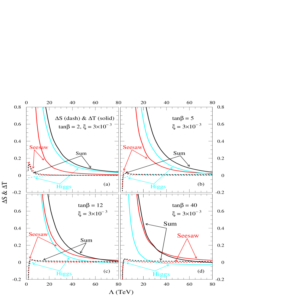
Figure 20: The contributions from the seesaw sector and the two-doublet-Higgs sector to the oblique parameters $T$ (solid curves) and $S$ (dashed curves).

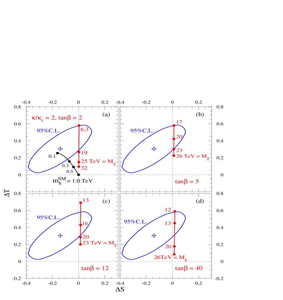
Figure 21: Top and bottom seesaw contributions to $\Delta S$ and $\Delta T$ are compared with the 95% C.L. error ellipse (with $m_{h}^{\rm ref}=1$ TeV) for $\kappa/\kappa_{c}=2$ and $\xi=3\times 10^{-3}$ with a variety of values of $\tan\beta$. The $\Delta S$-$\Delta T$ trajectories (including both Higgs and quark contributions) are shown as a function of $M_{\chi}$. For reference, the SM Higgs corrections to ($S$, $T$), relative to $m_{h}^{\rm ref}=1$ TeV, are depicted for $m_{h}^{\rm SM}$ varying from 100 GeV up to 1.0 TeV in plot (a).

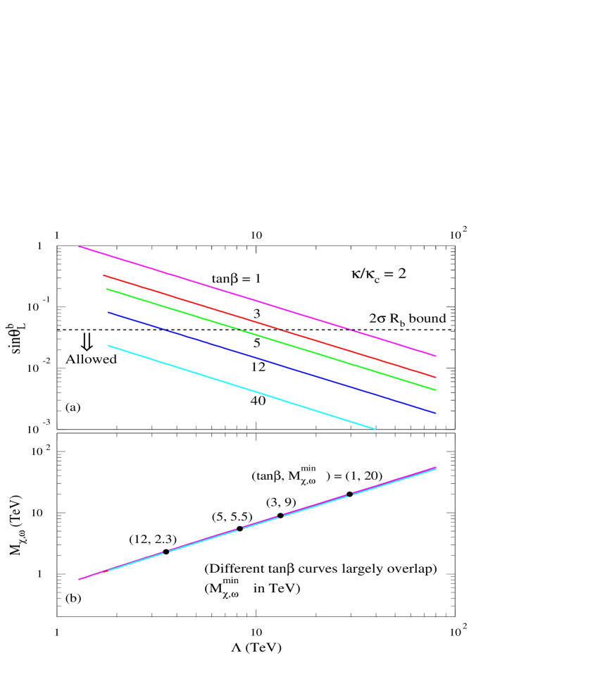
Figure 22: The $R_{b}$ limits are shown for the $b$ seesaw angle $s_{L}^{b}=\sin\theta_{L}^{b}$ in plot (a) and for the mass $M_{\omega}(\simeq M_{\chi})$ in plot (b). Here, we choose $\kappa/\kappa_{c}=2$ and a wide range of $\tan\beta$ values.

5 Conclusions

Electroweak symmetry breaking (EWSB) through the Top Quark Seesaw is an attractive mechanism that may naturally emerge from theories with bosonic extra dimensions. In this work, we have systematically investigated the Top Seesaw mechanism for generating the large top mass together with the full EWSB. We have applied the gap equation analysis to study the seesaw vacuum structure and determine the physical parameter space. With the Topcolor breaking scale ($\Lambda$) and the Topcolor gauge coupling ($h_{1}$) as inputs, and further imposing the physical values of the top mass ($m_{t}$) and the full EWSB VEV ($v$), we are able to predict all other seesaw parameters and thus the physical spectrum of the model from solving the seesaw gap equation. This includes the masses of singlet seesaw quark ${\chi}$ and the composite Higgs boson $h^{0}$. The Higgs mass $M_{h}$ is at the order of the seesaw mass gap $m_{t\chi}$, and typically around $\sim\!0.5-1$ TeV. The effective couplings, such as the Yukawa coupling $h$-$t$-$\overline{t}$ and gauge couplings $W$-$t$-$b$ and $Z$-$b$-$\overline{b}$, etc, are also analyzed, in comparison with their SM values.

The fermion content of the Top Seesaw is incomplete due to gauge anomalies, but a minimal choice of additional weak-singlet fermions, ${\omega}$, the seesaw partners for the bottom quark, renders the theory anomaly free and thus complete. This extended model contains two dynamical mass gaps $m_{t\chi}$ and $m_{b\omega}$ in the $(t{\chi})$ and $(b{\omega})$ channels, respectively. We have performed a complete analysis of the coupled seesaw gap equations in this extended model. The low energy theory contains two composite Higgs doublets. Topcolor instantons [7] are found to provide an economic and plausible mechanism for the mass generation of the pseudo-scalar $A^{0}$. In addition, they may also produce a significant part of the $b$ mass via the bottom seesaw. We have analyzed the resulting Higgs spectrum in this extended model by using two independent approaches. The Higgs mass spectrum typically contains the lightest $h^{0}$ with a mass around $\sim\!1$ TeV, and three other quite degenerate scalars, with masses around one to a few TeV. We also notice that this model has a particular simple limit, namely, when the seesaw quark ${\omega}$ becomes heavy enough and decouples from the low energy theory, it reduces back to the minimal Top seesaw model with a single Higgs doublet, and in this case, the bottom mass arises entirely from the Topcolor instanton contribution.

We have further analyzed the electroweak precision bounds on both the minimal and extended seesaw models. We find that it is generic in these models to have a small oblique parameter $S$, but a significantly positive seesaw contribution to $T$ that largely cancels with the negative $T$ from the heavy Higgs boson, in full consistency with the current $S-T$ bounds. This makes the dynamical Top seesaw models fully viable, and as a result, the current precision data is able to indirectly confine the heavy ${\chi}$ mass to the natural range of about ${\cal O}(3-10)$ TeV (for $\kappa/\kappa_{c}\leq 2$) in the minimal seesaw model. For the extended model with the bottom seesaw, the mass of the singlet seesaw quark ${\omega}$ is found to have good degeneracy with ${\chi}$. The $b-{\omega}$ mixing tends to reduce the seesaw contribution in $T$ (especially for the small to moderate $\tan\beta$ values), but the additional correction in the two-Higgs-doublet sector makes $T$ more positive and thus the final $S-T$ bounds appear at the similar level to that of the minimal model, i.e., the allowed seesaw quark masses $M_{{\chi},{\omega}}$ ranges from a few TeV up to $\sim\!30$ TeV for $1.05\mathrel{\vbox{\hbox{$<$}\nointerlineskip\hbox{$\sim$}}}\kappa/\kappa_{c}\mathrel{\vbox{\hbox{$<$}\nointerlineskip\hbox{$\sim$}}}4$. We have also analyzed the correction to the ${Zb\bar{b}}$ gauge coupling induced by the $b-{\omega}$ mixing and found that the $R_{b}$ measurement can put stronger bounds than the $T$ parameter only for very small $\tan\beta$ region, around $\tan\beta\mathrel{\vbox{\hbox{$<$}\nointerlineskip\hbox{$\sim$}}}2-3$.

So far, the Top seesaw mechanism, with necessary ingedients arising automatically in theories with bosonic extra dimensions, remains a most natural picture of the dynamical EWSB scenario, and is consistent with the current experimental data. In addition to successfully driving the full EWSB and providing the large top mass observed at the Tevatron, it has interesting phenomenological implications, including composite Higgs bosons, additional weak-singlet quarks in the TeV region, and, ultimately, an entire new layer of strong interaction forces at nearby scales to explore.

Acknowledgments
We thank many colleagues, especially R. Sekhar Chivukula, for discussions and reading the manuscript. HJH thanks the Fermilab Theory Group for invitations and support of his summer visits during which this collaboration was initiated and part of his work was performed. HJH was supported by the U.S. Department of Energy under Grant DE-FG03-93ER40757, CTH by the University Research Association for Fermilab under contract DE-AC02-76CHO3000 with the U.S. Department of Energy, and TT by the U.S. Department of Energy under contract W-31-109-Eng-38.

Appendices

Appendix A Equivalent Derivations of Top Seesaw Gap Equation

A.1 Exact Large-$N_{c}$ Gap Equation in the NJL-Formalism

In this Appendix, we derive the exact NJL seesaw gap equation in the large-$N_{c}$ limit based on the Schwinger-Dyson equation without mass-insertion, and prove it results in the same equation as the tadpole condition (66) in Sec. 2.4. Starting from the NJL vertex (41) in Sec. 2.2, we can write down the large-$N_{c}$ Schwinger-Dyson equation as shown in Fig. 23.

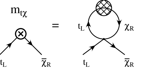
Figure 23: Exact large-$N_{c}$ Schwinger-Dyson equation for the NJL interaction in the minimal top seesaw model.

Then, we make use of the exact seesaw rotations in Eqs. (19)-(24) to transform the fields on both sides of the Schwinger-Dyson equation into the mass eigenbasis. The expanded diagrams are shown in Fig. 24 with proper rotation angles associated with each graph. The sums of the expanded diagrams on both sides should be equal to each other, and in particular, each expanded diagram in the upper plot of Fig. 24 must be equal to the sum of the two relevant expanded diagrams in the lower plot of Fig. 24 which share the same external lines. (One of two relevant diagrams in the lower plot of Fig. 24 has a $t^{\prime}$-loop and another has a ${\chi}^{\prime}$-loop.) This leads us to split the Schwinger-Dyson equation of Fig. 23 into four separate equations, which, however, take the following identical form,

$$m_{t\chi} = -\left[c_{L}s_{R}\Delta_{t}+c_{R}s_{L}\Delta_{\chi}\right]\,,$$ (129)

with

$$\Delta_{t}=-\displaystyle\frac{h_{1}^{2}N_{c}}{\Lambda^{2}}\,{\rm tr}\!\!\int\frac{dk^{4}}{2\pi^{4}}\frac{i}{~{}\backslash\!\!\!k-m_{t}}P_{R}\,,~{}~{}~{}~{}~{}\Delta_{\chi}=-\displaystyle\frac{h_{1}^{2}N_{c}}{\Lambda^{2}}\,{\rm tr}\!\!\int\frac{dk^{4}}{2\pi^{4}}\frac{i}{~{}\backslash\!\!\!k-M_{\chi}}P_{R}\,,$$ (130)

where $P_{L,R}=\left(1\mp\gamma_{5}\right)/2$. By a direct evaluation of the loop integrals $\Delta_{t}$ and $\Delta_{\chi}$ with the cutoff $\Lambda$, we can rewrite the Schwinger-Dyson equation (129) as,

$$\vspace*{3.5mm}m_{t\chi}~{}=~{}\frac{\kappa}{\kappa_{c}}\left\{c_{L}s_{R}\left(m_{t}-\frac{m_{t}^{3}}{\Lambda^{2}}\ln\left[\frac{\Lambda^{2}+m_{t}^{2}}{m_{t}^{2}}\right]\right)+s_{L}c_{R}\left(m_{\chi}-\frac{m^{3}_{\chi}}{\Lambda^{2}}\ln\left[\frac{\Lambda^{2}+m_{\chi}^{2}}{m_{\chi}^{2}}\right]\right)\right\}\,,$$ (131)

which is just the exact large-$N_{c}$ seesaw gap equation for $m_{t\chi}$, identical to the tadpole condition (66) in Sec. 2.4. This proves the equivalence between the NJL formalism and the Higgs tadpole formalism for deriving the seesaw gap equation.

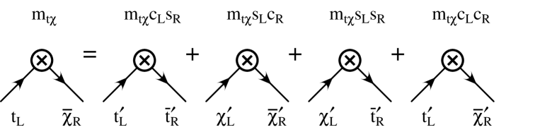
Figure 24: Diagrams expanded from both sides of the large-$N_{c}$ Schwinger-Dyson equation in Fig. 23, by using the exact seesaw rotations in Eqs. (19)-(24).

A.2 Mass-Insertion Gap Equation from Tadpole Condition

Here, we derive the tadpole condition with mass-insertion up to ${\cal O}(m_{t\chi}^{3})$ and prove it results in the same equation as the approximate NJL gap equation in Sec. 2.3. From the NJL interaction in Eq. (44), we introduce the auxiliary field $\Phi_{0}$ which, in the unitary gauge, takes the form of (61) with the VEV explicitly shifted. Then, the effective Lagrangian at the scale $\mu=\Lambda$ becomes,

$$\begin{array}[]{ll}{\cal L}_{\Lambda}&\!\!\!=-\left(\overline{t_{L}}~{}~{}\overline{\chi_{L}}\right)\left\lgroup\begin{array}[]{cc}m_{tt}&{m_{t\chi}}\\[5.69046pt] 0&{\overline{M}}\\ \end{array}\right\rgroup\left(\!\!\begin{array}[]{c}t_{R}\\ \chi_{R}\end{array}\!\!\right)-\displaystyle\frac{h_{1}}{\sqrt{2}}\overline{t_{L}}\left(c{\chi}_{R}+st_{R}\right)h_{0}+{\rm h.c.}-\frac{1}{2}\Lambda^{2}h_{0}^{2}-\Lambda^{2}v_{0}h_{0}\\[14.22636pt] \end{array}$$ (132)

where

$$m_{t\chi}=\displaystyle c\frac{h_{1}v_{0}}{\sqrt{2}}\,,~{}~{}~{}~{}m_{tt}=\displaystyle s\frac{h_{1}v_{0}}{\sqrt{2}}\,,~{}~{}~{}~{}\longrightarrow~{}~{}~{}~{}\frac{m_{tt}}{m_{t\chi}}=\frac{s}{c}\,,$$ (133)

and $s/c=\mu_{\chi t}/\mu_{\chi\chi}$ is the same as in Eq. (43). The diagonal mass-terms $m_{tt}$ ( ${\overline{M}}$ ) will be put into the $t$ (${\chi}$) propagator as usual, while the non-diagonal mass-term $m_{t\chi}$ can be included via the mass-insertion order by order. It is then straightforward to derive the tadpole condition $0=v_{0}\Lambda^{2}+\delta\widetilde{T}$ [similar to Eq. (65)] with $\delta\widetilde{T}$ computed from the one-loop Higgs tadpole diagrams. This is shown in Fig. 25, in which we perform the mass-insertion of $m_{t\chi}$ up to the third power. As a result, we derive a single condition on $m_{t\chi}$, which is identical to the gap equation (48) derived earlier in Sec. 2.3 by using the NJL formalism. This shows the equivalence between these two mass-insertion approaches.

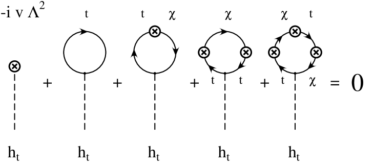
Figure 25: Higgs tadpole condition with mass-insertions to ${\cal O}(m_{t\chi}^{3})$.

Appendix B Potential Analysis for Higgs Mass Spectrum
with Bottom Seesaw

In this Appendix, we present an independent derivation of the composite Higgs spectrum by analyzing the Higgs potential in the extended model with a bottom seesaw. The potential analysis confirms the results derived in Sec. 3 where the Higgs masses are explicitly computed in the broken phase including the exact seesaw mass-diagonalizations. We start from the gauge-invariant Lagrangian $\,{\cal L}_{\rm mass}+{\cal L}_{\rm int}+{\cal L}_{\rm PQB}$ in Sec. 3 [cf. Eqs. (83), (84) and (87)], and evolve it down to the scale $\mu\left(<M_{{\chi},{\omega}}\leq\Lambda\right)$. We can thus derive the gauge-invariant effective Lagrangian with two dynamical Higgs-doublet fields and their interaction terms, up to ${\cal O}(\xi)$,

$$\begin{array}[]{ll}{\cal L}_{\mu<M_{{\chi},{\omega}}}\,=&-h_{1}\left[s_{t}\;\overline{\psi}t_{R}\Phi_{t0}+s_{b}\;\overline{\psi}b_{R}\Phi_{t0}+{\rm h.c.}\right]+Z_{t}|D_{\mu}\Phi_{t0}|^{2}+Z_{b}|D_{\mu}\Phi_{b0}|^{2}\\[8.53581pt] &+\xi\left(Z_{t}+Z_{b}\right)\epsilon^{\alpha\beta}\left[(D^{\mu}\Phi_{t0})^{\alpha}(D_{\mu}\Phi_{b0})^{\beta}+{\rm h.c.}\right]-V_{H}\,,\end{array}$$ (134)

where $(s_{t},\,s_{b})\equiv(\sin\theta_{t},\,\sin\theta_{b})$ and $(\tan\theta_{t},\,\tan\theta_{b})\equiv(\mu_{\chi t}/\mu_{\chi\chi},\,\mu_{\omega b}/\mu_{\omega\omega})$, with $(\theta_{t},\theta_{b})$ the partial rotation angles for $(t_{R},\,{\chi}_{R})$ and $(b_{R},\,{\omega}_{R})$ [cf. Eqs. (42)-(43) in Sec. 2.2]. The Higgs potential $V_{H}$ can be written as,

$$\begin{array}[]{ll}V_{H}\,=&\widetilde{M}_{t}^{2}|\Phi_{t0}|^{2}+\widetilde{M}_{b}^{2}|\Phi_{b0}|^{2}+\xi\widetilde{M}_{tb}^{2}\left[\epsilon^{\alpha\beta}\Phi_{t0}^{\alpha}\Phi_{b0}^{\beta}+{\rm h.c.}\right]+\widetilde{\lambda}_{t}(\Phi_{t0}^{\dagger}\Phi_{t0})^{2}+\widetilde{\lambda}_{b}(\Phi_{b0}^{\dagger}\Phi_{b0})^{2}\\[8.53581pt] &+\widetilde{\lambda}_{tb}(\Phi_{t0}^{\dagger}\Phi_{b0})(\Phi_{b0}^{\dagger}\Phi_{t0})+\xi\left[\widetilde{\lambda}_{t}^{\prime}|\Phi_{t0}|^{2}+\widetilde{\lambda}_{b}^{\prime}|\Phi_{b0}|^{2}\right]\left[\epsilon^{\alpha\beta}\Phi_{t0}^{\alpha}\Phi_{b0}^{\beta}+{\rm h.c.}\right],\end{array}$$

where the loop-induced Higgs mass terms and couplings are graphically defined in Fig. 26. For simplicity, the fermion lines of ${\chi}_{R}$ and ${\omega}_{R}$ represent the fields before the partial rotations mentioned above, but we keep in mind that such rotations just split each graph into two; this will not affect our current general derivation as is easy to check. From Eq. (B) and Fig. 26, we can derive three general relations, up to ${\cal O}(\xi)$,

$$\xi\widetilde{M}^{2}_{tb}=\xi\left[\widetilde{M}^{2}_{t}+\widetilde{M}^{2}_{b}-\Lambda^{2}\right],~{}~{}~{}~{}\widetilde{\lambda}_{t}^{\prime}=2\widetilde{\lambda}_{t}\,,~{}~{}~{}~{}\widetilde{\lambda}_{b}^{\prime}=2\widetilde{\lambda}_{b}\,.$$ (135)

The next step is to write down the renormalized Higgs potential, analyze the physical vacuum and derive the Higgs mass spectrum. So, we first express $V_{H}$ in terms of renormalized quantities,

$$\begin{array}[]{ll}V_{H}\,=&{M}_{t}^{2}|\Phi_{t}|^{2}+{M}_{b}^{2}|\Phi_{b}|^{2}+\xi{M}_{tb}^{2}\left[\epsilon^{\alpha\beta}\Phi_{t}^{\alpha}\Phi_{b}^{\beta}+{\rm h.c.}\right]+{\lambda}_{t}(\Phi_{t}^{\dagger}\Phi_{t})^{2}+{\lambda}_{b}(\Phi_{b}^{\dagger}\Phi_{b})^{2}\\[2.84526pt] &+{\lambda}_{tb}(\Phi_{t}^{\dagger}\Phi_{b})(\Phi_{b}^{\dagger}\Phi_{t})+\xi\left[{\lambda}_{t}^{\prime}|\Phi_{t}|^{2}+{\lambda}_{b}^{\prime}|\Phi_{b}|^{2}\right]\left[\epsilon^{\alpha\beta}\Phi_{t}^{\alpha}\Phi_{b}^{\beta}+{\rm h.c.}\right],\end{array}$$

with the following renormalization relations,

$$M_{t}^{2}=\widetilde{M}_{t}^{2}Z_{t}^{-1},~{}~{}~{}M_{b}^{2}=\widetilde{M}_{b}^{2}Z_{b}^{-1},~{}~{}~{}M_{tb}^{2}=\widetilde{M}_{tb}^{2}\left(Z_{t}Z_{b}\right)^{-\frac{1}{2}},$$

$$\lambda_{t}=\widetilde{\lambda}_{t}Z_{t}^{-2},~{}~{}~{}\lambda_{t}^{\prime}=\widetilde{\lambda}_{t}^{\prime}{Z_{t}^{-\frac{3}{2}}Z_{b}^{-\frac{1}{2}}},~{}~{}~{}\lambda_{b}=\widetilde{\lambda}_{b}Z_{b}^{-2},~{}~{}~{}\lambda_{b}^{\prime}=\widetilde{\lambda}_{b}^{\prime}{Z_{t}^{-\frac{1}{2}}Z_{b}^{-\frac{3}{2}}},~{}~{}~{}\lambda_{tb}=\widetilde{\lambda}_{tb}\left(Z_{t}Z_{b}\right)^{-1}.$$

where $(Z_{t},\,Z_{b})$ are the wavefunction renormalization constants of $(\Phi_{t0},\,\Phi_{b0})$, defined as, $\Phi_{t0}=Z_{t}^{-1/2}\Phi_{t}$ and $\Phi_{b0}=Z_{b}^{-1/2}\Phi_{b}$. Then, we can shift the VEVs of the two renormalized Higgs-doublets, $(\Phi_{t},\,\Phi_{b})$, similar Eq. (96) in Sec. 3.2. For the analysis of physical vacuum and the Higgs mass spectrum, it is convenient to choose the unitary gauge, in which the three physical combinations (orthogonal to the would-be Goldstone bosons) are defined as, $A^{0}=\sin\!\beta^{\prime}\pi_{b}^{0}+\cos\beta^{\prime}\pi_{t}^{0}$ and $H^{\pm}=\sin\!\beta^{\prime}\pi^{\pm}_{b}+\cos\!\beta^{\prime}\pi^{\pm}_{t}$, with $\tan\beta^{\prime}=(v_{t}+\xi v_{b})/(v_{b}+\xi v_{t})=\tan\beta+\xi(1-\tan\beta)+{\cal O}(\xi^{2})$.

Minimizing the effective Higgs potential $V_{H}$ in (B), we derive two extremum conditions,

$$\left[M_{t}^{2}+\lambda_{t}v_{t}^{2}\right]+\xi\cot\beta\left[M_{tb}^{2}+\frac{3}{2}\lambda_{t}^{\prime}v_{t}^{2}+\frac{1}{2}\lambda_{b}^{\prime}v_{b}^{2}\right] = 0\,,$$

$$\left[M_{b}^{2}+\lambda_{b}v_{b}^{2}\right]+\xi\tan\beta\left[M_{tb}^{2}+\frac{1}{2}\lambda_{t}^{\prime}v_{t}^{2}+\frac{3}{2}\lambda_{b}^{\prime}v_{b}^{2}\right] = 0\,,$$ (137)

which determine the physical vacuum and is formally equivalent to the gap equations (tadpole conditions) derived in Eq. (98) of Sec. 3.2. These conditions are needed in our derivation and can be used to simplify the mass formulae for the Higgs bosons. We start by extracting the $A^{0}$ mass term from Higgs potential (B) and obtain, up to ${\cal O}(\xi)$,

$$M^{2}_{A} = \frac{\xi}{2\sin\beta\,\cos\beta}\left[-2M_{tb}^{2}-\lambda_{t}^{\prime}v_{t}^{2}-\lambda_{b}^{\prime}v_{b}^{2}\right]=\frac{2\xi\Lambda^{2}}{\displaystyle\sin\!2\beta\sqrt{Z_{t}Z_{b}}}\,,$$ (138)

where we have used the minimal conditions in Eq. (B), and the relations in Eqs. (135) and (B). This result confirms our explicit one-loop calculation of $M_{A}$ in Eq. (109) of Sec. 3.3. We proceed by deriving the mass formulae for the neutral and charged Higgs bosons $(h_{t}^{0},\,h_{b}^{0},\,H^{\pm})$, which can be summarized up to ${\cal O}(\xi)$,

$$M_{11}^{2} \!\!=\!\! 2\lambda_{b}v_{b}^{2}+\displaystyle\xi\left[3\lambda_{b}^{\prime}v_{t}v_{b}-\tan\beta\left(M^{2}_{tb}+\frac{1}{2}\lambda_{t}^{\prime}v_{t}^{2}+\frac{3}{2}\lambda_{b}^{\prime}v_{b}^{2}\right)\right]$$ (139)

$$\simeq 4m_{b\omega}^{2}+\sin^{2}\!\beta\,M^{2}_{A}\,,$$

$$M_{22}^{2} \!\!=\!\! 2\lambda_{t}v_{t}^{2}+\displaystyle\xi\left[3\lambda_{t}^{\prime}v_{t}v_{b}-\cot\!\beta\left(M^{2}_{tb}+\frac{3}{2}\lambda_{t}^{\prime}v_{t}^{2}+\frac{1}{2}\lambda_{b}^{\prime}v_{b}^{2}\right)\right]$$ (140)

$$\simeq 4m_{t\chi}^{2}+\cos^{2}\!\beta\,M^{2}_{A}\,,$$

$$\xi M_{12}^{2} \!\!=\!\! \displaystyle\xi\left[M_{tb}^{2}+\frac{3}{2}\lambda_{t}^{\prime}v_{t}^{2}+\frac{3}{2}\lambda_{b}^{\prime}v_{b}^{2}\right]$$ (141)

$$\simeq -\sin\!\beta\,\cos\!\beta\;M^{2}_{A}+4\xi\left(m_{t\chi}^{2}+m_{b\omega}^{2}\right),$$

and

$$M^{2}_{H^{\pm}} = \frac{\lambda_{tb}}{2}\left[v_{t}\sin\!\beta^{\prime}+v_{b}\cos\!\beta^{\prime}\right]^{2}-\displaystyle\frac{\xi}{\sin\!2\beta}\left[2M_{tb}^{2}+\lambda_{t}^{\prime}v_{t}^{2}+\lambda_{b}^{\prime}v_{b}^{2}\right]$$ (142)

$$\simeq 2\left(m_{t\chi}^{2}+m_{b\omega}^{2}\right)+\left[M^{2}_{A}-4\xi\left(m_{t\chi}^{2}\cot\!\beta+m_{b\omega}^{2}\tan\!\beta\right)\right],$$

where mass notations of $M_{11,22,12}^{2}$ are the same as Eq. (106) in Sec. 3.3, and for simplification we have used the relation, $M_{\chi}\simeq M_{\omega}$, which results in $Z_{t}\simeq Z_{b}\simeq Z_{tb}/2$ and $\lambda_{t}\simeq\lambda_{b}\simeq\lambda_{tb}/2$. These are good approximations since the heavy masses $M_{\chi}$ and $M_{\omega}$ only affect them via weak logarithmic dependences (due to the decoupling theorem) and $M_{\chi}\simeq M_{\omega}$ is also justified from our physical seesaw solutions in Fig. 14. In summary, the above analysis agrees with our calculations in Sec. 3.3, and is particularly simple in extracting leading corrections at ${\cal O}(\xi)$. It is also remarkable that in this analysis we derive all relations in a rather general and formal manner in which no explicit one-loop calculation is needed for the quantities such as $Z_{t,b}$ and $\lambda_{t,b,tb}$ .

Figure 26: Effective mass terms and quartic self-couplings in the Higgs potential.

References

References

- [1] H.-C. Cheng, C. T. Hill, S. Pokorski and J. Wang, “The standard model in the latticized bulk”, hep-th/0104179.
- [2] C. T. Hill, S. Pokorski and J. Wang, “Gauge invariant effective Lagrangian for Kaluza-Klein modes”, hep-th/0104035.
- [3] W. A. Bardeen and R. B. Pearson, Phys. Rev. D 14, 547 (1976); W. A. Bardeen, R. B. Pearson and E. Rabinovici, Phys. Rev. D 21, 1037 (1980).
- [4] N. Arkani-Hamed, A. G. Cohen and H. Georgi, Phys. Rev. Lett. 86, 4757 (2001) [hep-th/0104005].
- [5] H. Cheng, C. T. Hill and J. Wang, “Dynamical electroweak breaking and latticized extra dimensions”, hep-ph/0105323.
- [6] N. Arkani-Hamed, A. G. Cohen and H. Georgi, “Electroweak symmetry breaking from dimensional deconstruction”, hep-ph/0105239.
- [7] C. T. Hill, Phys. Lett. B 345, 483 (1995) [hep-ph/9411426]; Phys. Lett. B 266, 419 (1991).
- [8] K. Lane and E. Eichten, Phys. Lett. B 352, 382 (1995) [hep-ph/9503433]; K. Lane, Phys. Lett. B 433, 96 (1998) [hep-ph/9805254].
- [9] B. A. Dobrescu and C. T. Hill, Phys. Rev. Lett. 81, 2634 (1998) [hep-ph/9712319]; R. S. Chivukula, B. A. Dobrescu, H. Georgi and C. T. Hill, Phys. Rev. D 59, 075003 (1999) [hep-ph/9809470].
- [10] B. A. Dobrescu, Phys. Lett. B 461, 99 (1999) [hep-ph/9812349]; H. Cheng, B. A. Dobrescu and C. T. Hill, Nucl. Phys. B 589, 249 (2000) [hep-ph/9912343], and hep-ph/0004072.
- [11] R. Jackiw and C. Rebbi, Phys. Rev. D 13, 3398 (1976); D. B. Kaplan, Phys. Lett. B 288, 342 (1992) [hep-lat/9206013].
- [12] N. Arkani-Hamed and M. Schmaltz, Phys. Rev. D 61, 033005 (2000) [hep-ph/9903417]; E. A. Mirabelli and M. Schmaltz, ibid. 61, 113011 (2000) [hep-ph/9912265]; D. E. Kaplan and T. M. Tait, JHEP0006, 020 (2000) [hep-ph/0004200]; G. Dvali and M. Shifman, Phys. Lett. B 475, 295 (2000) [hep-ph/0001072].
- [13] Y. Nambu, in Proceedings of Strong coupling gauge theories and beyond, pp.3-12, Nagoya, Japan, 1990.
- [14] V. A. Miransky, M. Tanabashi and K. Yamawaki, Mod. Phys. Lett. A 4, 1043 (1989).
- [15] W. A. Bardeen, C. T. Hill, and M. Lindner, Phys. Rev. D41, 1647 (1990).
- [16] For a recent review on top condensation, G. Cvetic, Rev. Mod. Phys. 71, 513 (1999) [hep-ph/9702381].
- [17] H. Collins, A. K. Grant and H. Georgi, Phys. Rev. D 61, 055002 (2000) [hep-ph/ 9908330].
- [18] R. S. Chivukula and C. Hölbling, Phys. Rev. Lett. 85, 511 (2000) [hep-ph/0002022].
- [19] M. E. Peskin and T. Takeuchi, Phys. Rev. Lett. 65, 964 (1990); Phys. Rev. D46, 381 (1992); W. J. Marciano and J. L. Rosner, Phys. Rev. Lett. 65, 2963 (1990); D. Kennedy and P. Langacker, ibid. 65, 2967 (1990); Phys. Rev. D 44, 1591 (1991); B. Holdom and J. Terning, Phys. Lett. B 247, 88 (1990); M. Golden and L. Randall, Nucl. Phys. B 361, 3 (1991); G. Altarelli and R. Barbieri, Phys. Lett. B 253, 161 (1991). G. Altarelli, R. Barbieri, and S. Jadach, Nucl. Phys. B 269, 3 (1992).
- [20] M. E. Peskin and J. D. Wells, hep-ph/0101342.
- [21] C. T. Hill, Phys. Rev. D 24, 691 (1981); B. Pendleton and G. G. Ross, Phys. Lett. B 98, 291 (1981). C. T. Hill, C. N. Leung and S. Rao, Nucl. Phys. B 262, 517 (1985).
- [22] H. Pagels and S. Stokar, Phys. Rev. D 20, 2947 (1979).
- [23] Y. Nambu and G. Jona-Lasinio, Phys. Rev. 122, 345 (1961).
- [24] C. T. Hill and D. S. Salopek, Annals Phys. 213, 21 (1992).
- [25] G. Buchalla, G. Burdman, C. T. Hill and D. Kominis, Phys. Rev. D 53, 5185 (1996) [hep-ph/9510376]; K. Lane, Phys. Rev. D 54, 2204 (1996) [hep-ph/9602221]; E. Eichten, K. Lane and J. Womersley, Phys. Rev. Lett. 80, 5489 (1998) [hep-ph/9802368]; E. Eichten, K. Lane and J. Womersley, Phys. Lett. B 405, 305 (1997) [hep-ph/9704455]; H.-J. He and C.-P. Yuan, Phys. Rev. Lett. 83, 28 (1998) [hep-ph/9810367]; G. Burdman, ibid. 83, 2888 (1999) [hep-ph/9905347]; G. Burdman, K. Lane and T. Rador, hep-ph/0012073.
- [26] M. L. Swartz, talk given at XIX International Symposium on Lepton and Photon Interactions at High Energies, August 9-14, 1999 [hep-ex/9912026].
- [27] K. Moenig, hep-ex/0101005, presentation at Linear Collider Workshop, Fermilab, Batavia, IL, USA, October, 2000; J. Erler, S. Heinemeyer, W. Hollik, G. Weiglein, and P. M. Zerwas, Phys. Lett. B486, 125 (2000); M. E. Peskin and J. D. Wells, hep-ph/0101342.
- [28] C. T. Hill, “Dynamical Symmetry Breaking of Electroweak Interactions and the Renormalization Group”, FERMI-CONF-90/170-T, presentation at the Workshop on Dynamical Symmetry Breaking, Nagoya, Japan, 1990; G. Cvetic, Rev. Mod. Phys. 71, 513 (1999).
- [29] B.A. Dobrescu, Phys. Rev. D 63, 015004 (2000) [hep-ph/9908391].
- [30] H. Georgi and H. D. Politizer, Phys. Rev. D14, 1829 (1976).
- [31] M. Bando, T. Kugo, N. Maekawa, N. Sasakura, K. Suehiro and Y. Watabiki, Phys. Lett. B246, 466 (1990).
- [32] T. Appelquist and J. Carrazone, Phys. Rev. D 11, 2856 (1975).
- [33] E.g., N. Maekawa, Phys. Rev. D52, 1684 (1995).
- [34] Particle Data Group, D. E. Groom et al., European Physical Journal C 15, 1 (2000), http://pdg.lbl.gov; LEP Electroweak Working Group, http://lepewwg.web.cern.ch; A. Gurtu, talk given at 30th International Conference on High Energy Physics, July 27-August 2, 2000, Osaka, Japan; M. W. Grünewald, “Electroweak Analysis”, presentation on behalf of LEP and SLD Collaborations, and the Electroweak Working Group, at LEP Physics Jamboree, CERN, Genève, July 10, 2001.
- [35] J. Erler, contribution to Workshop of QCD and Weak Boson Physics, Batavia, Illinois, June 1999 [hep-ph/0005084] and http://www.physics.upenn.edu/ erler/electroweak/ GAPP.html.
- [36] Hong-Jian He, T. Tait and C.-P. Yuan, Phys. Rev. D 62, 011702 (2000) (R), [hep-ph/9911266].
- [37] G. ’t Hooft, Phys. Rev. Lett. 37, 8 (1976); Phys. Rept. 142, 357 (1986).
- [38] H. E. Haber, hep-ph/9306207, presented at the Theoretical Advanced Study Institute, Boulder, Colorado, USA, June, 1992; H. E. Haber and H. E. Logan, Phys. Rev. D 62, 015011 (2000) [hep-ph/9909335]; and references therein.
- [39] H.-J. He, N. Polonsky and S. Su, Phys. Rev. D64, 053004 (2001) [hep-ph/0102144].
- [40] M. W. Grünewald, “Electroweak Analysis”, presentation on behalf of ALEPH, DELPHI, L3, OPAL and SLD Collaborations, and the Electroweak Working Group, at LEP Physics Jamboree, CERN, Genève, July 10, 2001.
- [41] E.g., A. Denner, R. J. Guth, W. Hollik, and J. H. Kuhn, Z. Phys. C51, 695 (1991).