hep-ph/0108032

IOA-TH.10/01

NTUA 06/01

On the stability of nontopological solitons in supersymmetric
extensions of the Standard Model: A Numerical Approach
G.K. Leontaris¹, A. Prikas², A. Spanou², N.D. Tracas², N.D. Vlachos^3
1Physics Department, University of Ioannina, Ioannina 45 110, Greece
²Physics Department, National Technical University, Athens 157 73 , Greece
³Physics Department, University of Thessaloniki, Thessaloniki 540 06, Greece
Abstract

In various supersymmetric extensions of the Standard Model there appear non-topological solitons due to the existence of $U(1)$ global symmetries associated with Baryon and/or Lepton quantum numbers. Trilinear couplings (A-terms) in the scalar potential break explicitly the $U(1)$ invariance. We investigate numerically the stability of these objects in the case that this breaking is small. We find that stable configurations, oscillating though, can still appear. Other relevant properties are also examined.  

July 2001

Non-topological solitons are non-dissipative solutions of finite energy which arise in field theories possessing continuous global symmetries [1],[2],[3]. Of particular interest are possible stable configurations which carry baryonic or leptonic charge [5] and appear in supersymmetric extensions of the Standard Model. In this latter context, they appear to have interesting cosmological consequences since they could be related to the baryon number of the universe, or even they could play a role as dark matter candidates [4]. In supersymmetric theories, the trilinear superpotential couplings of the matter and Higgs superfields, as well as the supersymmetry breaking terms, generate a scalar potential which may possess exact or approximate global symmetries which could be correlated to the above quantum numbers. It is the purpose of this letter to examine a generic form of such a scalar potential and investigate the properties of the solitonic configurations.

In general, the resulting scalar potential in a supersymmetric theory depends on various scalar fields, $U=U(\Phi_{1},\Phi_{2},\dots,\Phi_{n})$, however, in the present work we will concentrate on the simplest case of only one field $\Phi$, i.e. $U=U(\Phi)$, while the generalization is straightforward. The contributions from supersymmetry breaking and non-renormalizable terms in the scalar potential have the generic form 

$$U(\Phi) = m_{s}^{2}|\Phi|^{2}+\sum_{n}\left(\lambda_{NR}^{2}\frac{|\Phi|^{2(n-1)}}{M^{2(n-3)}}+A\frac{\Phi^{n}}{M^{n-3}}+A^{*}\frac{\Phi^{*n}}{M^{n-3}}\right)$$ (1)

In (1), $m_{s}$ is a soft mass term, of the order of the supersymmetry breaking scale. $\lambda_{NR}$ is a dimensionless constant associated to the Yukawa coupling of the corresponding non-renormalizable term of the superpotential. $A$ is the coefficient of the trilinear term in the scalar potential (the so-called $A$-term), while $M$ is of the order of the unification scale. It is easily observed [7] that in the case of a scalar potential with vanishing $A$-terms the global $U(1)$ symmetry of the Lagragian survives. Then, for appropriate values of the soft supersymmetry breaking parameters and Yukawas which determine the coefficients of the various potential terms, a stable solitonic configuration does appear. However, the $A$-terms are usually non-vanishing. Even if their initial value is zero, renormalization group running will generate a non-vanishing value and the aforementioned global $U(1)$ symmetry breaks. In this letter we wish to investigate the stability of the solitonic configuration in the presence of small non-zero $A$-terms which induce small perturbative terms in the scalar potential.

To this end, we will use a simplified model in $1+1$ dimensions and adopt the conventions and notations of reference [8]. Assuming a complex scalar filed $\Phi$, the dynamics of the resulting scalar field theory can be described by a Lagrangian density of the form

$${\cal L}=\frac{1}{2}\partial_{\mu}\Phi\partial^{\mu}\Phi^{*}-U(\Phi)$$ (2)

Starting with a potential respecting a $U(1)$ invariance

$$U(\Phi)=\frac{1}{2}m^{2}|\Phi|^{2}-\frac{1}{3}\alpha|\Phi|^{3}+\frac{1}{4}b|\Phi|^{4}$$ (3)

while making use of the rescalings [8]

$$\Phi\rightarrow\frac{m^{2}}{\alpha}\Phi,\quad\quad x\rightarrow\frac{x}{m}$$ (4)

one obtains the Lagrangian

$$\mathcal{L}=\frac{1}{2}\partial_{\mu}\Phi^{*}\partial^{\mu}\Phi-\frac{1}{2}|\Phi|^{2}+\frac{1}{3}|\Phi|^{3}-\frac{1}{4}B|\Phi|^{4}$$ (5)

with the parameter $B=\frac{bm^{2}}{\alpha^{2}}$. Note that in order to get the above Lagrangian we have divided by a factor $m^{6}/a^{2}$ which has dimensions of $m^{2}$. Therefore, the Lagrangian in (5) is dimensionless. The equation of motion reads

$$\ddot{\Phi}-\Phi^{\prime\prime}+\Phi-|\Phi|\Phi+B|\Phi|^{2}\Phi=0$$ (6)

Using the ansatz [3]

$$\Phi(x)=\sigma(x)e^{i\omega t}$$ (7)

and inserting (7) in (6) the following differential equation for $\sigma(x)$ is obtained

$$\sigma^{\prime\prime}+(\omega^{2}-1)\sigma+\sigma^{2}-B\sigma^{3}=0$$ (8)

The requirement for a finite energy configuration and the asymptotic behaviour at infinite “time”, $x\rightarrow\infty$, imply the following conditions for $\sigma$:

$$\sigma^{\prime}(0)=0,\quad\quad\sigma(\infty)=0.$$ (9)

The constraints imposed on $\omega$ by these conditions are written as

$$0<1-\frac{2}{9B}<\omega^{2}<1$$ (10)

The conserved charge is

$$Q=\frac{1}{2i}\int(\Phi^{*}\partial_{0}\Phi-\Phi\partial_{0}\Phi^{*})dx$$ (11)

Given the ansatz (7) one finds that the conserved charge is given by

$$Q=\omega\int\sigma(x)^{2}d\,x$$ (12)

Finally, the energy density is

$$\mathcal{E}=\frac{1}{2}|\dot{\Phi}|^{2}+\frac{1}{2}|\Phi^{\prime}|^{2}+\frac{1}{2}|\Phi|^{2}-\frac{1}{3}|\Phi|^{3}+\frac{1}{4}B|\Phi|^{4}$$ (13)

which, with the use of (7), becomes

$$\mathcal{E}=\frac{1}{2}\sigma^{\prime 2}+\frac{1}{2}(1+\omega^{2})\sigma^{2}-\frac{1}{3}\sigma^{3}+\frac{1}{4}B\sigma^{4}$$ (14)

A  numerical analysis of the model shows that static field configurations are obtained for a large portion of the parameter space $\omega^{2},B$. Finally, the extension in $2+1$ dimensions shows that similar static stable ‘objects’ do exist, at least for certain $\omega^{2}$-values [8].

We wish now to add a $U(1)$ breaking term in the (rescaled) Lagrangian (5) of the form

$$\frac{s}{n!}(\Phi^{n}+\Phi^{*n})$$ (15)

and examine in a similar manner the stability of the above configurations. We choose to work with $n=2$ and find that the equations of motion for the scalar field in this case generalize as follows

$$\ddot{\Phi}-\Phi^{\prime\prime}+\Phi-|\Phi|\Phi+B|\Phi|^{2}+2s\Phi^{*} = 0$$ (16)

$$\ddot{\Phi}^{*}-{\Phi^{*}}^{\prime\prime}+\Phi^{*}-|\Phi|\Phi^{*}+B|\Phi|^{2}+2s\Phi = 0$$ (17)

The current is given by $\Phi^{*}\partial_{\mu}\Phi-\Phi\partial_{\mu}\Phi^{*}$ and the charge $Q\propto\int(\Phi^{*}\partial_{0}\Phi-\Phi\partial_{0}\Phi^{*})d\,x$, respectively, however, due to the extra $U(1)$-breaking term the charge is no longer conserved. Its rate of change is given by

$$\frac{d\,Q}{d\,t} = \int is(\Phi^{2}-\Phi^{*2})\,d\,x$$ (18)

An analytic solution of the above system is hard to find, so our intention is to solve numerically the complete equations of motion, taking as starting point the ‘unperturbed’ solution (7).

We first check that our numerical methods reproduce the original results in the case of vanishing $s$-term ( the $U(1)$-invariant Lagrangian). Indeed, we have checked that the soliton-profile (the absolute value of the solution), to a very good approximation, remains constant in time while the charge, energy and energy/charge are constant within 2%, 1.4% and 0.02% correspondingly.

Next, we switch on the symmetry breaking term in the potential. In our numerical investigations we use the values $B=0.34$ and $\omega^{2}=0.51$ for the two potential parameters. In Fig.(1) we show the evolution of the profile in time, the oscillation of $|\Phi(x,t)|$ in time for four points ($x=0,2,5,7$) ($x=0$ is the top of the profile), and finally the parametric plot (Real Part, Imaginary Part) for the top of the profile. The last one is drawn for one period of the beat-like graph shown in the middle figure. The three rows correspond to three values of $s=0.007,0.003,0.001$.

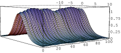
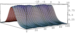
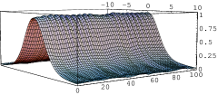
Figure 1: The time evolution of the soliton profile, the oscillation of the points $x=0,2,5,7$ and the parametric plot (Real Part, Imaginary Part) for one period and for three values of the breaking parameter $s=0.007,0.003,0.001$.

Some comments are in order. Although the $U(1)$ is explicitly broken, we see that we have a stable configuration though oscillating in time. We have checked the stability for a time corresponding to at least 10 periods ($2\pi/\omega$). All points of the profile oscillate in phase, while the “movement” of a point resembles a beat. The higher we are on the solitonic profile the larger the oscillation is. The parametric plot, which for a soliton is a circle, transforms to a “turning ellipse” which closes as a beat period is completed. As $s$ gets smaller, the oscillation decreases, the top of the profile becomes smooth with the time while in the parametric plot, the “turning ellipse” becomes a circle. The period of the beat remains constant (within numerical errors). The non-smooth ending of the profile for large $|x|$ is also due to numerical errors in the solution of the equation of motion.

It is interesting to analyze the real and the imaginary part of the solution, for $x=0$, as a function of time; this is shown in Fig.(2).

Figure 2: The real (left) and imaginary part of the solution as a function of time, for $x=0$ and $s=0.007$.

We see a clear oscillation with frequency $\omega$ which is modulated by a lower frequency. We clearly see the cosine and the sine function corresponding to the real and imaginary part (one should bear in mind that the ansatz for the solitonic configuration is $\sigma(x)\exp(i\omega t)$). The modulating signal has half a period phase difference between real and imaginary part. It is easy now to see that the high frequency of the beat-like profile is $2\omega$.

As the breaking parameter $s$ gets bigger, the oscillations show large amplitudes and the sense of a period fails to appear. This loss of clear periodicity starts to appear when the ratio energy/charge, which also oscillates with time, becomes larger than one, which is the constraint for a stable configuration against decaying to the fundamental mesons of the theory.

At this point, we should explain what we mean by charge. In the $U(1)$ invariant theory the conserved charge is defined by the Eq.(11). We continue to define the charge by the same equation, in the sense that our symmetry breaking parameter is small. The energy is given by Eq.(11), where of course we have added the term coming from the breaking, namely $(1/6)sRe[\Phi^{2}]$. The lack of periodicity is most clearly seen in the parametric plot (Real Part, Imaginary Part) where now the line tends to cover all the plane, exhibiting two “fixed points”. In Fig(3) we show the parametric plot for $x=0$, $s=0.015$ and for $t=300$. The “fixed points” could be attributed to a left over $Z_{2}$ symmetry. Indeed, the symmetry breaking term $\Phi^{n}+\Phi^{*n}$ shows a $Z_{n}$ symmetry if $\Phi=\sigma(x)\exp(i\omega t)$.

Figure 3: Parametric plot (Real Part, Imaginary Part), for $x=0$, $s=0.015$ and for $t=300$

We have made a Fourier analysis of the real and imaginary part of the complete solution for $x=0$ and, as it is obvious from the Figures, we get large amplitudes just for two frequencies which are multiplets of the basic frequency ($2\pi/T$, where $T$ is the period of the beat) namely $\omega$, which has the largest amplitude and $\omega^{\prime}=\omega\pm(2\pi/T)$. To a very good approximation we can write

$$\Phi(x=0,t)=c_{R}\cos(\omega t)+c^{\prime}_{R}\cos(\omega^{\prime}t)+i(c_{I}\sin(\omega t)+c^{\prime}_{I}\sin(\omega^{\prime}t))$$ (19)

where the $c$’s are constant coefficients. Since all points oscillate in phase we can write for the complete solution

$$\Phi(x,t)=K(x)\Phi(0,t)$$ (20)

where $K(x)$ is an unknown function of the position. The first obvious choice for $K(x)$ is $\sigma(x)$ itself. We have tried therefore the solution

$$\Phi(x,t)=\frac{\sigma(x)}{\sigma(0)}\Phi(0,t)$$ (21)

which for the central region of the profile differs from the numerical solution by as low as 2%. Fourier analysis can also help to understand the transition to the simple solution, Eq.(7). As $s\rightarrow 0$, the amplitude of the $\omega^{\prime}$ frequency gets smaller and the only surviving frequency is the $\omega$.

The above analysis holds when the parameters $B$ and $\omega$ of the solution are deep inside the stability region of the $(B,\omega^{2})$ space. The stability region is defined from the Eq.(10) [8]. When we are near the boundary, the situation gets extremely complicated. Even with a relatively small breaking parameter $s$, the energy/charge ratio becomes larger than 1. The period of the beat is no more constant but depends on the value of $s$. The Fourier analysis of the solution shows that more than two frequencies have large amplitudes and, for large enough $s$, none of them is equal to $\omega$. As $s\rightarrow 0$, all the amplitudes, except one, tend to zero, while the remaining one corresponds to a frequency which tends to $\omega$ (since the beat period is not constant, the basic frequency of the Fourier analysis, and therefore its multiplets also change).

We get a more clear situation near the boundary of the stable solutions, in the case of the so called thin wall approximation: the function $\sigma(x)$ has a constant value for a certain region in $x$ and zero elsewhere. In that case, the Euler-Lagrange equation, the current and the energy density of the soliton are given respectively:

$$\ddot{\Phi}+\Phi-|\Phi|\Phi+B{|\Phi|}^{2}\Phi+2s\Phi^{\ast}=0$$ (22)

$$j^{0}=\frac{1}{2i}({\Phi}^{\ast}\dot{\Phi}-\Phi{\dot{\Phi}}^{*})$$ (23)

$$\mathcal{E}=\frac{1}{2}|\dot{\Phi}|^{2}+\frac{1}{2}|\Phi|^{2}-\frac{1}{3}{|\Phi|}^{3}+\frac{B}{4}{|\Phi|}^{4}+\frac{s}{2}(\Phi^{2}+\Phi^{\ast 2})$$ (24)

The absence of spatial derivative terms in the energy makes the soliton more stable. We have found that on the boundary, the beat frequency is proportional to the only free parameter of the (rescaled) Lagrangian, namely $B$, taking care always to keep the breaking parameter $s$ low enough to avoid the energy/charge ratio to become greater than 1. We have also checked that the same behaviour persists when we add a $\Phi^{6}$ term in the $U(1)$ preserving potential.

A last point to mention is the tremendously different situation we are facing in the case we change the power of the symmetry breaking term Eq.(15) in the Lagrangian to $n=3$. In Fig.(4) we show the parametric plot for the same values of the parameters, $B=0.34$, $\omega^{2}=0.51$ and for $s=0.05$.

Figure 4: Parametric plot (Real Part, Imaginary Part), in the case where the breaking term is $\Phi^{3}+\Phi^{*3}$ and for $x=0$, $s=0.05$ and for $t=100$

Although the graph seems chaotic with respect to the corresponding one in the previous case, we clearly see three “fixed points”. A larger $s$ value is also needed, with respect to the previous case again, in order to see a significant disturbance of the soliton profile. There appears again a $\Phi(x,t)$ which is periodic in time, but it does not show a beat-like shape and the period seems smaller than before. We are planning to make a more general presentation of these points in a forthcoming publication.

In conclusion, motivated by the $U(1)$ breaking symmetry terms that appear in the soft-term Lagrangian, we investigated the simple case of a complex scalar field, in 1+1 dimensions, possessing a non-topological solition-type solution, with an extra explicitly breaking term. We solve numerically the equation of motion and found an oscillating with time qball-like solution. The points of the profile oscillate with a beat-like movement showing stability in time. As the breaking parameter gets larger and the oscillating energy/charge ratio gets greater than 1, instability appears in the solution in the sense of non constant period and with the destruction of the beat-like shape.

We would like to thank P. Dimopoulos, K. Farakos, A. Kehagias and G. Koutsoumbas, G. Tiktopoulos for helpful discussions.

References

- [1] R. Friedberg, T. D. Lee and A. Sirlin, “A Class Of Scalar - Field Soliton Solutions In Three Space Dimensions,” Phys. Rev. D 13 (1976) 2739.
- [2] T. D. Lee and Y. Pang, “Nontopological solitons,” Phys. Rept. 221 (1992) 251.
- [3] S. Coleman, “Q Balls,” Nucl. Phys. B 262 (1985) 263 [Erratum-ibid. B 269 (1985) 744].
- [4] A. Kusenko and M. Shaposhnikov, “Supersymmetric Q-balls as dark matter,” Phys. Lett. B 418 (1998) 46 [hep-ph/9709492].
- [5] A. Kusenko, “Small Q balls,” Phys. Lett. B 404 (1997) 285 [hep-th/9704073].
- [6] K. Enqvist and J. McDonald, “B-ball baryogenesis and the baryon to dark matter ratio,” Nucl. Phys. B 538 (1999) 321 [hep-ph/9803380].
- [7] M. Axenides, E. G. Floratos, G. K. Leontaris and N. D. Tracas, “Q-balls and the proton stability in supersymmetric theories,” Phys. Lett. B 447 (1999) 67 [hep-ph/9811371].
- [8] M. Axenides, S. Komineas, L. Perivolaropoulos and M. Floratos, Phys. Rev. D 61 (2000) 085006 [hep-ph/9910388].