MADPH 01-1235

BNL-HET-01/28

MSUHEP-10709

DFTT 19/2001

hep-ph/0108030

Gluon-fusion contributions to $H+2$ jet production

V. Del Duca^a, W. Kilgore^b, C. Oleari^c, C. Schmidt^d and D. Zeppenfeld^{c (a)} I.N.F.N., Sezione di Torino via P. Giuria, 1 - 10125 Torino, Italy
^(b) Physics Department, Brookhaven National Laboratory, Upton, New York 11973, U.S.A.
^(c) Department of Physics, University of Wisconsin, Madison, WI 53706, U.S.A.
^(d) Department of Physics and Astronomy, Michigan State University, East Lansing, MI 48824, U.S.A.

Real emission corrections to Higgs production via gluon fusion, at order $\alpha_{s}^{4}$, lead to a Higgs plus two-jet final state. We present the calculation of these scattering amplitudes, as induced by top-quark triangle-, box- and pentagon-loop diagrams. These diagrams are evaluated analytically for arbitrary top mass $m_{t}$. We study the renormalization and factorization scale-dependence of the resulting $H+2$ jet cross section, and discuss phenomenologically important distributions at the LHC. The gluon fusion results are compared to expectations for weak-boson fusion cross sections.

1 Introduction

Gluon fusion and weak-boson fusion are expected to be the most copious sources of Higgs bosons in $pp$-collisions at the Large Hadron Collider (LHC) at CERN. Beyond representing the most promising discovery processes [1, 2], these two production modes are also expected to provide a wealth of information on Higgs couplings to gauge bosons and fermions [3]. The extraction of Higgs boson couplings, in particular, requires precise predictions of production cross sections.

Next-to-leading order (NLO) QCD corrections to the inclusive gluon-fusion cross section are known to be large, leading to a $K$-factor close to two [4]. Because the lowest order process is loop induced, a full NNLO calculation would entail a three-loop evaluation, which presently is not feasible. In the intermediate Higgs mass range, which is favored by electroweak precision data [5], the Higgs boson mass $m_{H}$ is small compared to the top-quark pair threshold and the large $m_{t}$ limit promises to be an adequate approximation. Consequently, present efforts on a NNLO calculation of the inclusive gluon-fusion cross section concentrate on the $m_{t}\,\mbox{$\rightarrow$}\,\infty$ limit, in which the task reduces to an effective two-loop calculation [6]. In order to assess the validity of this approximation, gluon-fusion cross-section calculations, which include all finite $m_{t}$ corrections, are needed. Of particular interest are phase space regions where one or several of the kinematical invariants are of the order of, or exceed, the top-quark mass, i.e. regions of large Higgs boson or jet transverse momenta, or regions where dijet invariant masses become large. For larger Higgs boson masses, top-mass corrections become important and a full calculation of $H+2$ jet production is needed.

A key component of the program to measure Higgs boson couplings at the LHC is the weak-boson fusion (WBF) process, $qq\mbox{$\rightarrow$}qqH$ via $t$-channel $W$ or $Z$ exchange, characterized by two forward quark jets [3]. QCD radiative corrections to WBF are known to be small [7] and, hence, this process promises small systematic errors. $H+2$ jet production via gluon fusion, while part of the inclusive Higgs signal, constitutes a background when trying to isolate the $HWW$ and $HZZ$ couplings responsible for the WBF process. A precise description of this background is needed in order to separate the two major sources of $H+2$ jet events: one needs to find characteristic distributions which distinguish the weak boson fusion process from gluon fusion. One such feature is the typical large invariant mass of the two quark jets in WBF. A priori, this large kinematic invariant, $m_{jj}^{2}\gg 4m_{t}^{2}$, invalidates the heavy top approximation and requires a full evaluation of all top-mass effects. We will find, however, that even in this phase-space region the large $m_{t}$ limit works extremely well, provided that jet transverse momenta remain small compared to $m_{t}$.

In a previous letter [8] we presented first results of our evaluation of the real-emission corrections to gluon fusion which lead to $H+2$ parton final states, at order $\alpha_{s}^{4}$. The contributing subprocesses include quark-quark scattering which involves top-quark triangles, quark-gluon scattering processes which are mediated by top-quark triangles and boxes, and gluon scattering which requires pentagon diagrams in addition. The purpose of this paper is to provide details of our calculation and to give a more complete discussion of its phenomenological implications. In Section 2, we start with a brief overview of the calculation. Full expressions for the quark-quark and the quark-gluon scattering amplitudes are given in Section 3. Expressions for the $gg\mbox{$\rightarrow$}ggH$ amplitudes, which were obtained by symbolic manipulation, are too long to be given explicitly. Instead we describe the details of the calculational procedure in Section 3.3. The matrix elements for all subprocesses have been checked both analytically and numerically. The most important of these tests are described in Section 4. We then turn to numerical results, in particular to implications for LHC phenomenology. In Section 5, we first compare overall $H+2$ jet cross sections from weak-boson fusion and from gluon fusion and determine the subprocess decomposition of the latter. QCD uncertainties are assessed via a discussion of the scale dependence (renormalization and factorization) of our results. We investigate various distributions, searching for characteristic differences between gluon fusion and WBF. Our final conclusions are given in Section 6.

A number of technical details are collected in the Appendixes. Scalar integrals, in particular the evaluation of scalar five-point functions, are discussed in Appendix A. Appendix B gives useful relations among Passarino-Veltman $C_{ij}$ and $D_{ij}$ functions. Finally, in Appendixes C, D, and E, we provide expressions for the color decomposition and the tensor integrals encountered in triangle, box and pentagon graphs.

2 Outline of the calculation

The production of a Higgs boson in association with two jets, at order $\alpha_{s}^{4}$, can proceed via the subprocesses

$$qq\,\mbox{$\rightarrow$}\,qqH\;,\qquad qQ\,\mbox{$\rightarrow$}\,qQH\;,\qquad qg\,\mbox{$\rightarrow$}\,qgH\;,\qquad gg\,\mbox{$\rightarrow$}\,ggH\;,$$ (2.1)

and all crossing-related processes. Here the first two entries denote scattering of identical and non-identical quark flavors. In Fig. 1 we have collected a few representative Feynman diagrams which contribute to subprocesses with four, two and zero external quarks. In our calculation, the top quark is treated as massive, but we neglect all other quark masses, so that the Higgs boson only couples via a top-quark loop. Typically we have a $ggH$ coupling through a triangle loop (Fig. 1 (a)), a $gggH$ coupling mediated by a box loop (Fig. 1 (b)) and a $ggggH$ coupling which is induced through a pentagon loop (Fig. 1 (c)). The number and type of Feynman diagrams can be easily built from the simpler dijet QCD production processes at leading order. One needs to insert the Higgs-gluon “vertices” into the tree-level diagrams for $2\,\mbox{$\rightarrow$}\,2$ QCD parton scattering in all possible ways.

     

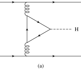
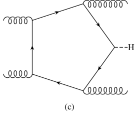
Figure 1: Examples of Feynman graphs contributing to $H+2$ jet production via gluon fusion.

In the following counting, we exploit Furry’s theorem, i.e. we are counting as one the two charge-conjugation related diagrams where the loop momentum is running clockwise and counter-clockwise. This halves the number of diagrams. In addition, the crossed processes are not listed as extra diagrams, but are included in the final results. Three distinct classes of processes need to be considered.

1. $qq\,\mbox{$\rightarrow$}\,qqH$ and $qQ\,\mbox{$\rightarrow$}\,qQH$ There are only 2 diagrams obtained from the insertion of a triangle loop into the tree-level diagrams for $qq\,\mbox{$\rightarrow$}\,qq$. One of them is depicted in Fig. 1 (a), while the other is obtained by interchanging the two identical final quarks. In the case of $qQ\,\mbox{$\rightarrow$}\,qQH$, where $Q$ is a different flavor, there is only one diagram, i.e. Fig. 1 (a).

2. $qg\,\mbox{$\rightarrow$}\,qgH$ At tree level, there are 3 diagrams contributing to the process $qg\,\mbox{$\rightarrow$}\,qg$: one with a three-gluon vertex and two Compton-like ones. Inserting a triangle loop into every gluon line, we have a total of 7 different diagrams. In addition, we can insert a box loop into the diagram with the three-gluon vertex, in 3 different ways: the $3!$ permutations of the 3 gluons are reduced to 3 graphs by using Furry’s theorem. In total we have 10 different diagrams for the $qg\,\mbox{$\rightarrow$}\,qgH$ scattering amplitude.

3. $gg\,\mbox{$\rightarrow$}\,ggH$ Four diagrams contribute to the tree-level scattering process $gg\,\mbox{$\rightarrow$}\,gg$: a four-gluon vertex diagram and 3 diagrams with two three-gluon vertices each. Inserting a triangle loop in any of the gluonic legs gives rise to 19 different diagrams. The insertion of the box loop in the 3 diagrams with three-gluon vertices yields another 18 diagrams. Finally, there are 12 pentagon diagrams (corresponding to $4!$ permutations of the external gluons, divided by 2, according to Furry’s theorem).

The amplitudes for these processes are ultraviolet and infrared finite in $D=4$ dimensions. Nevertheless, we kept $D$ arbitrary in several parts of our computation because some functions are divergent in $\epsilon=(4-D)/2$ at intermediate steps. Obviously, these divergences cancel when the intermediate expressions are combined to give final amplitudes. An example of this behavior is given by Eqs. (C.9) and (C.10), where the divergent part of the $B_{0}$ functions cancels among the different contributions to the triangle graphs.

Given the large number of contributing Feynman graphs, it is most convenient to give analytic results for the scattering amplitudes for fixed polarizations of the external quarks and gluons. These amplitudes are then evaluated numerically, instead of using trace techniques to express polarization averaged squares of amplitudes in terms of relativistic invariants. We proceed to derive explicit expressions for these amplitudes.

3 Notation and matrix elements

Within the SM, the effective interaction of the Higgs boson with gluons is dominated by top-quark loops because the top Yukawa coupling, $h_{t}=m_{t}/v$ with $v=246.22$ GeV, is much larger than the $Hb\bar{b}$ coupling. In the following we only consider top-loop contributions. All the $H+4$ parton amplitudes, at lowest order, are then proportional to $h_{t}\,g_{s}^{4}$, where $g_{s}=\sqrt{4\pi\alpha_{s}}$ is the SU(3) coupling strength. It is convenient to absorb these coupling constants into an overall factor

$$F=h_{t}\;{g_{s}^{4}\over 16\pi^{2}}\;4\,m_{t}=4\,{m_{t}^{2}\over v}\,\alpha_{s}^{2}\;,$$ (3.1)

where we have anticipated the loop factor $1/16\pi^{2}$ and the emergence of an explicit factor, $4\,m_{t}$, from all top-quark loops, which results from the compensation of the chirality flip, induced by the insertion of a single scalar $Ht\bar{t}$ vertex.

3.1 $qQ\,\mbox{$\rightarrow$}\,qQH$ and $qq\,\mbox{$\rightarrow$}\,qqH$

The simplest contribution to $H+2$ jet production is provided by the $qQ\,\mbox{$\rightarrow$}\,qQH$ process depicted in Fig. 1(a). Other four-quark amplitudes are obtained by crossing. We neglect external fermion masses and use the formalism and the notation of Ref. [9] for the spinor algebra. For a subprocess like

$$q(\overline{p}_{1},i_{1})+\overline{Q}(\overline{p}_{4},i_{4})\,\mbox{$\rightarrow$}\,q(\overline{p}_{2},i_{2})+\overline{Q}(\overline{p}_{3},i_{3})+H(P)\,,$$ (3.2)

with

$$\overline{p}_{1}^{2}=\overline{p}_{2}^{2}=\overline{p}_{3}^{2}=\overline{p}_{4}^{2}=0,\qquad P^{2}=m^{2}_{H},$$ (3.3)

each external (anti-)fermion is described by a two-component Weyl-spinor of chirality $\tau=\sigma_{i}=S_{i}\overline{\sigma}_{i}$,

$$\psi(\overline{p}_{i},\overline{\sigma}_{i})_{\tau}=S_{i}\sqrt{2\,\overline{p}_{i}^{0}}\,\delta_{\sigma_{i}\tau}\chi_{\sigma_{i}}(\overline{p}_{i})\;.$$ (3.4)

Here $\overline{p}_{i}$, $\overline{\sigma}_{i}$ and $i_{i}$ denote the physical momentum, the helicity and the color index of the quark or anti-quark, and the sign factor $S_{i}$ allows for an easy switch between fermions ($S_{i}=+1$) and anti-fermions ($S_{i}=-1$). The quark-gluon vertices of Fig. 1(a), including the attached gluon propagators, are captured via the effective quark currents

$$J_{21}^{\mu}=\delta_{\sigma_{2}\sigma_{1}}\;\chi^{\dagger}_{\sigma_{2}}(\overline{p}_{2})(\sigma^{\mu})_{\tau}\chi_{\sigma_{1}}(\overline{p}_{1}){1\over(p_{1}-p_{2})^{2}}=\delta_{\sigma_{2}\sigma_{1}}\;\left<2\right|(\sigma^{\mu})_{\tau}\left|1\right>{1\over(p_{1}-p_{2})^{2}}$$ (3.5)

and

$$J_{43}^{\mu}=\delta_{\sigma_{4}\sigma_{3}}\;\left<4\right|(\sigma^{\mu})_{\tau}\left|3\right>{1\over(p_{3}-p_{4})^{2}}\;.$$ (3.6)

Here we have used helicity conservation via the assignments $\tau=\sigma_{1}=\sigma_{2}$ and $\tau=\sigma_{3}=\sigma_{4}$, respectively, and the sign factors for the fermions provide an easy connection between the gluon momenta $q_{1}=p_{2}-p_{1}$ and $q_{2}=p_{4}-p_{3}$ going out of the top-quark triangle and the physical quark momenta $\overline{p}_{i}=S_{i}p_{i}$. Finally we have used the shorthand notation

$$\left|1\right> = \chi_{\sigma_{1}}(\overline{p}_{1})\;,$$

$$\left<2\right| = \chi^{\dagger}_{\sigma_{2}}(\overline{p}_{2})\;,$$

$$\left|3\right> = \chi_{\sigma_{3}}(\overline{p}_{3})\;,$$

$$\left<4\right| = \chi^{\dagger}_{\sigma_{4}}(\overline{p}_{4})\;,$$ (3.7)

and $(\sigma^{\mu})_{\pm}=(1,\pm$$\sigma$) is the reduction of Dirac matrixes $\gamma^{\mu}$ into the two-component Weyl basis. Since the quark currents $J_{12}^{\mu}$ and $J_{43}^{\mu}$ are conserved, we have

$$J_{12}^{\mu}\left(p_{1}-p_{2}\right)_{\mu}=0,\qquad J_{34}^{\mu}\left(p_{3}-p_{4}\right)_{\mu}=0\;.$$ (3.8)

The Weyl spinors and the currents $J_{21}$ and $J_{43}$ are easily evaluated numerically [9]. The scattering amplitude for different flavors on the two quark lines is then given by

$${\cal A}^{qQ}=F^{qQ}J_{21}^{\mu}J_{43}^{\nu}T_{\mu\nu}(q_{1},q_{2})\,t^{a}_{i_{2}i_{1}}\,t^{a}_{i_{4}i_{3}}={\cal A}_{2143}^{qQ}\,t^{a}_{i_{2}i_{1}}\,t^{a}_{i_{4}i_{3}}\;,$$ (3.9)

where the overall factor

$$F^{qQ}=S_{1}\,S_{2}\,S_{3}\,S_{4}\;4\sqrt{\overline{p}_{1}^{0}\,\overline{p}_{2}^{0}\,\overline{p}_{3}^{0}\,\overline{p}_{4}^{0}}\;F$$ (3.10)

includes the normalization factors of external quark spinors. The $t^{a}_{ij}={\lambda^{a}_{ij}/2}$ are the color generators in the fundamental representation of SU$(N)$, $N=3$. As detailed in Appendix C, the tensor $T_{\mu\nu}(p,q)$ can be written as

$$T^{\mu\nu}(p,q) = F_{T}\left(p^{2},q^{2},(p+q)^{2}\right)\,\left(p\cdot q\,g^{\mu\nu}-p^{\nu}\,q^{\mu}\right)$$ (3.11)

$$+ F_{L}\left(p^{2},q^{2},(p+q)^{2}\right)\,\left(q^{2}p^{2}g^{\mu\nu}-p^{2}\,q^{\mu}\,q^{\nu}-q^{2}\,p^{\mu}\,p^{\nu}+p\cdot q\,p^{\mu}q^{\nu}\right)\;.$$

Analytic expressions for the scalar form factors $F_{T}$ and $F_{L}$ are given in Eqs. (C.9) and (C.10).

The scattering amplitude for two identical quarks is obtained from the result above by including Pauli interference, which results from interchanging quarks 2 and 4,

$${\cal A}^{qq}={\cal A}_{2143}^{qq}\,t^{a}_{i_{2}i_{1}}\,t^{a}_{i_{4}i_{3}}-{\cal A}_{4123}^{qq}\,t^{a}_{i_{4}i_{1}}\,t^{a}_{i_{2}i_{3}}\;.$$ (3.12)

The squared amplitude, summed over initial- and final-particle color, becomes

$$\sum_{\rm col}|{\cal A}^{qq}|^{2}=\left(|{\cal A}_{2143}|^{2}+|{\cal A}_{4123}|^{2}\right)\frac{N^{2}-1}{4}+2\mathop{\rm Re}\left({\cal A}_{2143}{\cal A}_{4123}^{*}\right)\frac{N^{2}-1}{4N}.$$ (3.13)

The squared amplitude for the $qQ\,\mbox{$\rightarrow$}\,qQH$ process can be read from Eq. (3.13) by putting ${\cal A}_{4123}=0$.

3.2 $qg\,\mbox{$\rightarrow$}\,qgH$

          

         

           

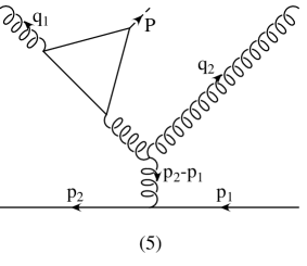
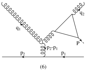
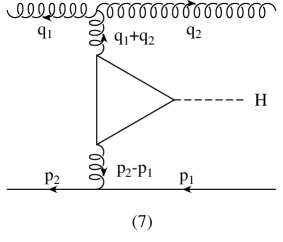
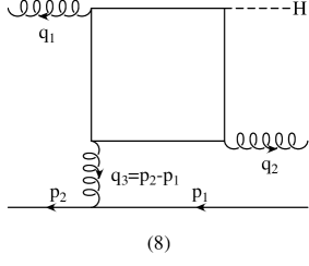
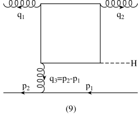
Figure 2: Feynman graphs contributing to the process $qg\mbox{$\rightarrow$}qgH$. Graphs (3) and (4) are the same as (1) and (2), but with gluon labels interchanged. No distinction is made between the two orientations of the fermion arrow on the top-quark loop, because they are related by Furry’s theorem.

Twenty distinct Feynman graphs contribute to the process

$$g(\overline{q}_{1},a_{1})+q(\overline{p}_{1},i_{1})\,\mbox{$\rightarrow$}\,g(\overline{q}_{2},a_{2})+q(\overline{p}_{2},i_{2})+H(P)\;,$$ (3.14)

and crossing related processes (the color index of the external gluons is indicated with $a_{i}$). However, pairs with opposite directions of the top-quark fermion arrow in the loop are related by charge conjugation and will not be counted separately in the following (see Appendixes C and D).

The resulting ten Feynman graphs are depicted in Fig. 2. Following Ref. [9], all gluon momenta are treated as outgoing. For the specific process of Eq. (3.14) we then set $q_{1}=-\overline{q}_{1}$ and $q_{2}=+\overline{q}_{2}$, with

$$\overline{p}_{1}^{2}=\overline{p}_{2}^{2}=\overline{q}_{1}^{2}=\overline{q}_{2}^{2}=0,\qquad P^{2}=m^{2}_{H}.$$ (3.15)

Feynman graphs with a triangle insertion in an external gluon line, i.e. with one light-like gluon attached to the top-quark triangle, receive contributions from a single form factor, $F_{T}$, only (see Eq. (C.12)). These simplifications are best captured by replacing the polarization vectors $\epsilon_{i}^{\mu}=\epsilon_{i}^{\mu}(\overline{q}_{i})$ with the effective polarization vectors

$$e^{\mu}_{iH}=F_{T}\left(0,\left(P+q_{i}\right)^{2},P^{2}\right){1\over\left(P+q_{i}\right)^{2}}\left(q_{i}^{\mu}\,\epsilon_{i}\cdot P-\epsilon_{i}^{\mu}\,q_{i}\cdot P\right)\;,$$ (3.16)

for gluons $i=1,2$, with $F_{T}$ given in Eq. (C.10).

External quark lines are handled as for the $qQ\mbox{$\rightarrow$}qQH$ amplitudes. Feynman graphs 5 through 10 are proportional to the quark current $J_{21}^{\mu}$ defined in Eq. (3.5). Spinor normalization factors are absorbed into the overall factor

$$F^{qg}=-S_{1}S_{2}\,2\sqrt{\overline{p}_{1}^{0}\,\overline{p}_{2}^{0}}\;F\;\delta_{\sigma_{1}\sigma_{2}}\;.$$ (3.17)

Using the shorthand notation [9]

$$\left<2,q_{i}\right| = \chi^{\dagger}_{\sigma_{2}}(\overline{p}_{2})(\epsilon\hskip-4.05904pt\hbox to4.05904pt{\hss$/$\hss}_{i})_{\sigma_{2}}(p\hskip-5.03125pt\hbox to5.03125pt{\hss$/$\hss}_{2}+q\hskip-4.8229pt\hbox to4.8229pt{\hss$/$\hss}_{i})_{-\sigma_{2}}{1\over(p_{2}+q_{i})^{2}}\;,$$ (3.18)

$$\left|q_{i},1\right> = (p\hskip-5.03125pt\hbox to5.03125pt{\hss$/$\hss}_{1}-q\hskip-4.8229pt\hbox to4.8229pt{\hss$/$\hss}_{i})_{-\sigma_{1}}(\epsilon\hskip-4.05904pt\hbox to4.05904pt{\hss$/$\hss}_{i})_{\sigma_{1}}\chi_{\sigma_{1}}(\overline{p}_{1}){1\over(p_{1}-q_{i})^{2}}\;,$$ (3.19)

for the 2-component Weyl spinors describing emission of a gluon next to an external quark, we arrive at a compact notation for the contributions to the $qg\,\mbox{$\rightarrow$}\,qgH$ scattering amplitude

$${\cal A}^{qg}\!\!\!\! = \!\!\!{\cal A}^{qg}_{\mu_{1}\mu_{2}}\,\epsilon_{1}^{\mu_{1}}\,\epsilon_{2}^{\mu_{2}}$$ (3.20)

$$= \!\!\!\!F^{qg}\Bigg{\{}\!\!\left(t^{a_{1}}t^{a_{2}}\right)_{i_{2}i_{1}}\Big{[}\left<2\right|(e\hskip-4.65627pt\hbox to4.65627pt{\hss$/$\hss}_{1H})_{\sigma_{1}}\left|q_{2},1\right>+\left<2,q_{1}\right|(e\hskip-4.65627pt\hbox to4.65627pt{\hss$/$\hss}_{2H})_{\sigma_{1}}\left|1\right>\Big{]}+$$

$$\phantom{\!\!\!\!F^{qg}\Bigg{\{}\!\!}\left(t^{a_{2}}t^{a_{1}}\right)_{i_{2}i_{1}}\Big{[}\left<2\right|(e\hskip-4.65627pt\hbox to4.65627pt{\hss$/$\hss}_{2H})_{\sigma_{1}}\left|q_{1},1\right>+\left<2,q_{2}\right|(e\hskip-4.65627pt\hbox to4.65627pt{\hss$/$\hss}_{1H})_{\sigma_{1}}\left|1\right>\Big{]}+$$

$$\phantom{\!\!\!\!F^{qg}\Bigg{\{}\!\!}\left[t^{a_{1}},t^{a_{2}}\right]_{i_{2}i_{1}}\Biggl{[}\mbox{}+2\Big{(}J_{21}\cdot q_{2}\,e_{1H}\cdot\epsilon_{2}-J_{21}\cdot e_{1H}\,\left(p_{2}-p_{1}\right)\cdot\epsilon_{2}-J_{21}\cdot\epsilon_{2}\,q_{2}\cdot e_{1H}\Big{)}$$

$$\phantom{\!\!\!\!F^{qg}\Bigg{\{}\!\!\left[t^{a_{1}},t^{a_{2}}\right]_{i_{2}i_{1}}\biggl{[}}-2\Big{(}J_{21}\cdot q_{1}\,e_{2H}\cdot\epsilon_{1}-J_{21}\cdot e_{2H}\,\left(p_{2}-p_{1}\right)\cdot\epsilon_{1}-J_{21}\cdot\epsilon_{1}\,q_{1}\cdot e_{2H}\Big{)}$$

$$\phantom{\!\!\!\!F^{qg}\Bigg{\{}\!\!\left[t^{a_{1}},t^{a_{2}}\right]_{i_{2}i_{1}}\Biggl{[}}-\left[\left(\frac{\left(q_{1}+q_{2}\right)\cdot\left(p_{1}-p_{2}\right)}{(q_{1}+q_{2})^{2}}F_{T}-\left(p_{1}-p_{2}\right)^{2}F_{L}\right)J_{21}^{\mu}+\frac{J_{21}\cdot P}{(q_{1}+q_{2})^{2}}F_{T}\,P^{\mu}\right]$$

$$\phantom{\!\!\!\!F^{qg}\Bigg{\{}\!\!\left[t^{a_{1}},t^{a_{2}}\right]_{i_{2}i_{1}}\biggl{[}-\Bigg{[}}\times\Big{[}\epsilon_{1}\cdot\epsilon_{2}\,\left(q_{2}-q_{1}\right)_{\mu}-2\,q_{2}\cdot\epsilon_{1}\,\epsilon_{2\mu}+2\,q_{1}\cdot\epsilon_{2}\,\epsilon_{1\mu}\Big{]}$$

$$\phantom{\!\!\!\!F^{qg}\Bigg{\{}\!\!\left[t^{a_{1}},t^{a_{2}}\right]_{i_{2}i_{1}}\biggl{[}}-B_{\mu_{1}\mu_{2}\mu_{3}}\,\epsilon_{1}^{\mu_{1}}\,\epsilon_{2}^{\mu_{2}}\,J_{21}^{\mu_{3}}\Biggr{]}\Bigg{\}}$$

where $F_{T}=F_{T}\left(\left(q_{1}+q_{2}\right)^{2},\left(p_{1}-p_{2}\right)^{2},P^{2}\right)$, and analogously for $F_{L}$.

The contributions of the box diagrams enter in the last line of Eq. (3.20) via the tensor $B_{\mu_{1}\mu_{2}\mu_{3}}=B_{\mu_{1}\mu_{2}\mu_{3}}(q_{1},q_{2},q_{3})$ (with $q_{3}=p_{2}-p_{1}$). Gauge invariance and Bose symmetry of the gluons limit the relevant structure of these box contributions to just two independent scalar functions, as we will now show.

It is easy to see that the $qg\,\mbox{$\rightarrow$}\,qgH$ amplitude ${\cal A}^{qg}$ is invariant under the replacements $\epsilon_{1}^{\mu}\,\mbox{$\rightarrow$}\,\epsilon_{1}^{\mu}+\kappa_{1}q_{1}^{\mu}$ and $\epsilon_{2}^{\mu}\,\mbox{$\rightarrow$}\,\epsilon_{2}^{\mu}+\kappa_{2}q_{2}^{\mu}$, for arbitrary constants $\kappa_{i}$. By proper choice of these constants, the polarization vectors of the two on-shell gluons can be made orthogonal to both $q_{1}$ and $q_{2}$. This can be seen by introducing a convenient basis of Minkowski space, composed of the vectors $q_{1}^{\mu}$, $q_{2}^{\mu}$ and

$$x^{\mu} = q_{2}\cdot q_{3}\,q_{1}^{\mu}+q_{1}\cdot q_{3}\,q_{2}^{\mu}-q_{1}\cdot q_{2}\,q_{3}^{\mu}\;,$$ (3.21)

$$y^{\mu} = \epsilon^{\mu\alpha\beta\rho}q_{1\alpha}\,q_{2\beta}\,q_{3\rho}\;.$$ (3.22)

The vector $y^{\mu}$ is orthogonal to all momenta occurring in the boxes ($q_{1},q_{2}$ and $q_{3}$) while $x^{\mu}$ is orthogonal to $q_{1}^{\mu}$, $q_{2}^{\mu}$ and $y^{\mu}$. More precisely

$$x\cdot x = {\rm det}{\cal Q}_{3}\equiv q_{1}\cdot q_{2}\Bigl{[}q_{3}^{2}\;q_{1}\cdot q_{2}-2\;q_{1}\cdot q_{3}\;q_{2}\cdot q_{3}\Bigr{]}\;,$$ (3.23)

$$y\cdot y = {\rm det}{\cal Q}_{3}\;,$$ (3.24)

$$x\cdot q_{1} = 0\;,\qquad x\cdot q_{2}=0\;,\qquad x\cdot q_{3}=-{{\rm det}{\cal Q}_{3}\over q_{1}\cdot q_{2}}\;,$$ (3.25)

$$y\cdot q_{1} = 0\;,\qquad y\cdot q_{2}=0\;,\qquad y\cdot q_{3}=0\;,\qquad y\cdot x=0\;,$$ (3.26)

where ${\rm det}{\cal Q}_{3}$ denotes the Gram determinant of the box, i.e. the determinant of the $3\times 3$ matrix with elements $\left({\cal Q}_{3}\right)_{ij}=-q_{i}\cdot q_{j}$. Obviously ${\rm det}{\cal Q}_{3}$ is symmetric under interchange of the three gluon labels. The non-symmetric form given in Eq. (3.23) pertains to our particular situation where only $q_{3}$ may be off-shell ($q_{1}^{2}=q_{2}^{2}=0$).

In the following we take

$$\epsilon_{1}^{\mu} = \frac{x^{\mu}}{\sqrt{-{\rm det}{\cal Q}_{3}}}\,,$$ (3.27)

$$\epsilon_{2}^{\mu} = \frac{y^{\mu}}{\sqrt{-{\rm det}{\cal Q}_{3}}}\,,$$ (3.28)

as the two independent polarization vectors of each of the on-shell gluons. With this choice, we eliminate the two $B_{c}$ contributions in the box tensor $B_{\mu_{1}\mu_{2}\mu_{3}}$ (see Eq. (D.6)) since they contain a factor $q_{1}^{\mu_{2}}$ or $q_{2}^{\mu_{1}}$, which vanishes upon contraction with the polarization vectors.

We can then write the squared element for $qg\,\mbox{$\rightarrow$}\,qgH$, summed over the polarization vectors of the external gluons in the form

$$\sum_{\rm pol}|{\cal A}^{qg}|^{2}=\left({1\over{\rm det}{\cal Q}_{3}}\right)^{2}\left[|{\cal A}_{xx}^{qg}|^{2}+|{\cal A}_{xy}^{qg}|^{2}+|{\cal A}_{yx}^{qg}|^{2}+|{\cal A}_{yy}^{qg}|^{2}\right]\;,$$ (3.29)

where the shorthand ${\cal A}_{xy}^{qg}={\cal A}^{qg}_{\mu_{1}\mu_{2}}\,x^{\mu_{1}}\,y^{\mu_{2}}$, etc. has been used. Expressions for the contracted tensor integrals for the boxes that appear in Eq. (3.20) are given in Eqs. (D.15)–(D.20).

In addition, the color structure of the $qg\mbox{$\rightarrow$}qgH$ amplitude is given by (see Eq. (3.20))

$${\cal A}^{qg}=(t^{a_{1}}t^{a_{2}})_{i_{2}i_{1}}{\cal A}^{qg}_{12}+(t^{a_{2}}t^{a_{1}})_{i_{2}i_{1}}{\cal A}^{qg}_{21}\;,$$ (3.30)

so that the resulting color-summed squared amplitude takes the form

$$\sum_{\rm col}|{\cal A}^{qg}|^{2}=\left(|{\cal A}^{qg}_{12}|^{2}+|{\cal A}^{qg}_{21}|^{2}\right)\frac{\left(N^{2}-1\right)^{2}}{4N}-2\mathop{\rm Re}\left[{\cal A}^{qg}_{12}\left({\cal A}^{qg}_{21}\right)^{*}\right]\frac{N^{2}-1}{4N}\;.$$ (3.31)

3.3 $gg\,\mbox{$\rightarrow$}\,ggH$

For the process

$$g(\overline{q}_{1},a_{1})+g(\overline{q}_{2},a_{2})\,\mbox{$\rightarrow$}\,g(\overline{q}_{3},a_{3})+g(\overline{q}_{4},a_{4})+H(P)\;,$$ (3.32)

we introduce the outgoing momenta $q_{i}$, so that $q_{1}=-\overline{q}_{1}$, $q_{2}=-\overline{q}_{2}$, $q_{3}=+\overline{q}_{3}$ and $q_{4}=+\overline{q}_{4}$, where

$$\overline{q}_{1}^{2}=\overline{q}_{2}^{2}=\overline{q}_{3}^{2}=\overline{q}_{4}^{2}=0,\qquad P^{2}=m_{H}^{2},$$ (3.33)

and $a_{i}$ are the color indices in the adjoint representation carried by the gluons.

Due to the large number of diagrams and the length of the results, we are not going to write explicitly the expressions for the amplitude, but we describe in detail the procedure we follow.

We used QGRAF [10] to generate the 49 diagrams for this process. As detailed in Sec. 2, these diagrams are obtained by the insertion of a triangle, a box or a pentagon loop into the tree-level diagrams for $gg\,\mbox{$\rightarrow$}\,gg$ scattering, so that we can write the un-contracted amplitude in the “formal” way

$$\left({\cal A}^{gg}\right)_{\alpha\beta\gamma\delta}\equiv\sum_{i=1}^{19}c_{i}^{T}\,T^{i}_{\alpha\beta\gamma\delta}+\sum_{i=1}^{18}c_{i}^{B}\,B^{i}_{\alpha\beta\gamma\delta}+\sum_{i=1}^{12}c_{i}^{P}\,P^{i}_{\alpha\beta\gamma\delta}.$$ (3.34)

where the tensor functions $T^{i}$, $B^{i}$ and $P^{i}$ are Feynman diagrams that contain a triangle, a box and a pentagon fermionic loop, while $c_{i}^{T},c_{i}^{B}$ and $c_{i}^{P}$ are the respective color factors. This amplitude will be contracted with the external polarization vectors of the gluons, $\epsilon_{i}$, to give

$${\cal A}^{gg}=\epsilon_{1}^{\alpha}\,\epsilon_{2}^{\beta}\,\epsilon_{3}^{\gamma}\,\epsilon_{4}^{\delta}\,\left({\cal A}^{gg}\right)_{\alpha\beta\gamma\delta}\equiv\left({\cal A}^{gg}\right)_{\epsilon_{1}\epsilon_{2}\epsilon_{3}\epsilon_{4}}.$$ (3.35)

We used Maple to trace over the Dirac $\gamma$ matrixes and to manipulate the expressions. Since the Higgs couples as a scalar to the massive top quark in the loop, the resulting trace in the numerator of the generic $n$-point function has at most $n-1$ loop-momentum factors. Using the tensor-reduction procedure described by Passarino and Veltman [11], we can express the triangle and box one-loop tensor integrals in terms of the external momenta $q_{i}^{\mu}$ and in terms of the scalar functions $C_{ij}$ ($i=1\ldots 2,\ j=1\ldots 4$) and $D_{ij}$ ($i=1\ldots 3,\ j=1\ldots 13$). For speed reasons, we preferred not to express directly the final amplitude in terms of scalar triangles and boxes (the $C_{0}$ and $D_{0}$ functions in Passarino-Veltman notation), in our Monte Carlo program. Expressions for the amplitude written in terms of the $C_{0}$ and $D_{0}$ integrals are considerably larger than the result where we keep the $C_{ij}$ and $D_{ij}$ functions.

In dealing with diagrams with a pentagon loop, we worked directly with the dot products in the numerator. In fact, the generic tensor pentagon appearing in $gg\,\mbox{$\rightarrow$}\,ggH$ scattering has the form

$$E(p_{1},p_{2},p_{3},p_{4})^{\{\alpha,\ \alpha\beta,\ \alpha\beta\gamma,\ \alpha\beta\gamma\delta\}}=$$

$${}\int\frac{d^{D}k}{i\pi^{D/2}}\frac{\{k^{\alpha},\ k^{\alpha}k^{\beta},\ k^{\alpha}k^{\beta}k^{\gamma},\ k^{\alpha}k^{\beta}k^{\gamma}k^{\delta}\}}{[k^{2}-m_{t}^{2}][(k+p_{1})^{2}-m_{t}^{2}][(k+p_{12})^{2}-m_{t}^{2}][(k+p_{123})^{2}-m_{t}^{2}][(k+p_{1234})^{2}-m_{t}^{2}]},$$

where $p_{ij}=p_{i}+p_{j}$, and similar ones for $p_{ijl}$ and $p_{ijln}$, and where the set of $p_{i}$, $\{p_{1},p_{2},p_{3},p_{4}\}$, is one of the 24 permutations of the external gluon momenta $\{q_{1},q_{2},q_{3},q_{4}\}$. These permutations are reduced to 12, once Furry’s theorem is taken into account. The generic scalar five-point function, that is Eq. (3.3) with a 1 in the numerator, will be indicated with $E_{0}(p_{1},p_{2},p_{3},p_{4})$.

The tensor indices appearing in the numerator are always contracted with one of the following:

1. the metric tensor $g^{\mu\nu}$

2. one of the external momenta $q_{i}^{\mu}$

3. one of the external polarization vector $\epsilon_{i}^{\mu}$.

The procedure we have used in these three cases is the following.

1. Every time there is a $k^{2}=k^{\alpha}k^{\beta}g_{\alpha\beta}$ product in the numerator, we write it as

   $$k^{2}=\left[k^{2}-m_{t}^{2}\right]+m_{t}^{2},$$ (3.37)

   and the first term is going to cancel the first propagator, giving rise to a four-point function, while the last one will multiply the rest of the tensor structure in the numerator, that now has been reduced by two powers of the loop momentum $k$.

2. We rewrite every scalar product of the type $(k\cdot q_{i})$ in the numerator as a difference of two propagators, using the identity

   $$k\cdot q_{i}=\frac{1}{2}\left\{\left[\left(k+p+q_{i}\right)^{2}-m_{t}^{2}\right]-\left[\left(k+p\right)^{2}-m_{t}^{2}\right]-2\,q_{i}\cdot p\right\},$$ (3.38)

   where $p$ is an arbitrary momentum. The first two terms in the sum are going to cancel the two propagators adjacent to the external gluon leg with momentum $q_{i}$, while the last one will contribute to the rest of the tensor structure in the numerator, now reduced by one power of $k$.

3. When the dot product $(k\cdot\epsilon_{i})$ appears in the numerator, we choose the four external gluon momenta as our basis of Minkowski space. Hence we can expand the external polarization vector $\epsilon_{i}$ as

   $$\epsilon_{i}^{\mu}=\sum_{j=1}^{4}\epsilon_{ij}\,q_{j}^{\mu},\qquad i=1\ldots 4,$$ (3.39)

   where the coefficients $\epsilon_{ij}$ are computed by inverting the system of equations

   $$\epsilon_{i}\cdot q_{k}=-\sum_{j=1}^{4}\epsilon_{ij}\,\left({\cal Q}_{4}\right)_{jk},\qquad i,k=1\ldots 4,$$ (3.40)

   where the elements of the matrix ${\cal Q}_{4}$ are given by

   $$\left({\cal Q}_{4}\right)_{jk}=-q_{j}\cdot q_{k}.$$ (3.41)

   Using Eq. (3.39), we can rewrite every scalar product of the form $(k\cdot\epsilon_{i})$ in the numerator of the Feynman diagrams as a sum over $(k\cdot q_{j})$, that we handle in the same way as shown in Eq. (3.38).

   The matrix ${\cal Q}_{4}$ is singular when the four gluons become planar, i.e. when the four gluon momenta cease to be linearly independent. This can easily be seen in the center-of-mass frame of partons 1 and 2, where we can write

   $$q_{1} = E\left(1,0,0,1\right),$$

   $$q_{2} = E\left(1,0,0,-1\right),$$

   $$q_{3} = E_{3}\left(1,\sin\theta,0,\cos\theta\right),$$

   $$q_{4} = E_{4}\left(1,\sin\theta^{\prime}\cos\phi,\sin\theta^{\prime}\sin\phi,\cos\theta^{\prime}\right),$$

   and the determinant of the matrix ${\cal Q}_{4}$ becomes

   $$\det{\cal Q}_{4}=-4E^{4}E_{3}^{2}E_{4}^{2}\left(1-\cos^{2}\theta^{\prime}\right)\left(1-\cos^{2}\theta\right)\left(1-\cos^{2}\phi\right).$$ (3.42)

   The cuts imposed on the final-state partons (see Eq. (5.1)) avoid the singular region when one of the final-state partons is collinear with the initial-beam direction (singularities in $\theta$ and $\theta^{\prime}$).

   The singularity in $\phi$ is un-physical, and the final amplitude should be finite near the singular points $\phi_{S}=0,\pi$. In our FORTRAN program, when the Monte Carlo integration approaches the singular points in $\phi$, we interpolate the value we need from the values of the amplitude in the points $\phi=\phi_{S}\pm 0.01\,\pi$. We have checked that the interpolated amplitude differs from the exact value of the amplitude by less than $1\%$, in the non-singular region.

By iterating this reduction procedure, we can write the contracted amplitude for $gg\,\mbox{$\rightarrow$}\,ggH$ scattering in terms of

• twelve $E_{0}(p_{a},p_{b},p_{c},p_{d})$ functions, i.e. the scalar five-point functions computed in different kinematics;

• twelve permutations of $D_{ij}$ functions with argument $D_{ij}(p_{a},p_{b},p_{c})$, with $a<c$, six $D_{ij}(p_{a},p_{b}+p_{c},p_{d})$ with $a<d$ and twelve $D_{ij}(p_{a},p_{b},p_{c}+p_{d})$, together with the corresponding $D_{0}$ functions;

• three $C_{ij}(p_{a}+p_{b},p_{c}+p_{d})$, and four $C_{ij}(p_{a},p_{b}+p_{c}+p_{d})$, together with the corresponding $C_{0}$ functions.

As usual, the set $\{p_{a},p_{b},p_{c},p_{d}\}$ is chosen in the group of permutations of the gluon momenta $\{q_{1},q_{2},q_{3},q_{4}\}$. To reduce the number of the $D_{ij}$ and $C_{ij}$ functions to this independent set, we made use of some identities between these functions, that we collect in Appendix B.

As stated in Eq. (3.34), we can study the color factors of the $gg\,\mbox{$\rightarrow$}\,ggH$ process, by dividing the full amplitude into three different classes, according to the number of fermionic propagators in the loop. We first discuss the color factors of the diagrams containing a pentagon loop.

• Diagrams with a pentagon loop
  The contribution from the sum of charge-conjugated pentagon diagrams is proportional to the sum of two color traces with four $t$ matrixes (see Eq. (E)). From the invariance property of the trace under cyclic permutations, we have only $(4-1)!=6$ independent traces, from the permutation of the four gluon indices. These six color traces combine together as in Eq. (E) to give rise to three independent color structures

  $$c_{1} = {\rm Tr}\left(t^{a_{1}}t^{a_{2}}t^{a_{3}}t^{a_{4}}\right)+{\rm Tr}\left(t^{a_{1}}t^{a_{4}}t^{a_{3}}t^{a_{2}}\right)$$

  $$c_{2} = {\rm Tr}\left(t^{a_{1}}t^{a_{3}}t^{a_{4}}t^{a_{2}}\right)+{\rm Tr}\left(t^{a_{1}}t^{a_{2}}t^{a_{4}}t^{a_{3}}\right)$$ (3.43)

  $$c_{3} = {\rm Tr}\left(t^{a_{1}}t^{a_{4}}t^{a_{2}}t^{a_{3}}\right)+{\rm Tr}\left(t^{a_{1}}t^{a_{3}}t^{a_{2}}t^{a_{4}}\right).$$

  The $c_{i}$ color coefficients are real. In fact, using the identity (the sum over the repeated index is understood)

  $${\rm Tr}\left(t^{a_{1}}t^{a_{2}}t^{a_{3}}t^{a_{4}}\right)=\frac{1}{4N}\delta^{a_{1}a_{2}}\delta^{a_{3}a_{4}}+\frac{1}{8}\left(d^{a_{1}a_{2}l}+i\,f^{a_{1}a_{2}l}\right)\left(d^{a_{3}a_{4}l}+i\,f^{a_{3}a_{4}l}\right),$$ (3.44)

  where $f$ is the (totally antisymmetric) SU$(N)$ structure constant and $d$ is the totally symmetric symbol, we can write, for example,

  $$c_{1}=\frac{1}{4}\left[\frac{2}{N}\delta^{a_{1}a_{2}}\delta^{a_{3}a_{4}}+d^{a_{1}a_{2}l}d^{a_{3}a_{4}l}-f^{a_{1}a_{2}l}f^{a_{3}a_{4}l}\right],$$ (3.45)

  and similar ones for $c_{2}$ and $c_{3}$. Since $f$ and $d$ are real constants, the $c_{i}$ are real too.

  A few useful identities can be derived if we take the differences of the $c_{i}$

  $$c_{1}-c_{2}=-\frac{1}{2}f^{a_{1}a_{2}l}f^{a_{3}a_{4}l}\quad\Longrightarrow\quad f^{a_{1}a_{2}l}f^{a_{3}a_{4}l}=2\,(c_{2}-c_{1}),$$

  $$c_{3}-c_{1}=-\frac{1}{2}f^{a_{1}a_{4}l}f^{a_{2}a_{3}l}\quad\Longrightarrow\quad f^{a_{1}a_{4}l}f^{a_{2}a_{3}l}=2\,(c_{1}-c_{3}),$$ (3.46)

  $$c_{2}-c_{3}=-\frac{1}{2}f^{a_{1}a_{3}l}f^{a_{4}a_{2}l}\quad\Longrightarrow\quad f^{a_{1}a_{3}l}f^{a_{4}a_{2}l}=2\,(c_{3}-c_{2}).$$

  Note that the differences of the $c_{i}$ in the system (- ‣ 3.3) automatically embodies the Jacobi identity: by summing the three expressions, we have

  $$f^{a_{1}a_{2}l}f^{a_{3}a_{4}l}+f^{a_{1}a_{4}l}f^{a_{2}a_{3}l}+f^{a_{1}a_{3}l}f^{a_{4}a_{2}l}=0.$$ (3.47)

• Diagrams with a box loop
  These diagrams all contain a three-gluon vertex together with the quark loop. Since the sum of the charge-conjugated boxes is proportional to the structure constant $f$ (see Eq. (D)), the final color factors accompanying these diagrams are a product of two $f$’s, such as $f^{a_{1}a_{2}l}f^{a_{3}a_{4}l}$.

  With the help of Eq. (- ‣ 3.3), we can express these products in terms of differences of the $c_{i}$ color factors.

• Diagrams with a triangle loop
  The same argument can be used to show that the color structure of all the diagrams with a three-point function insertion are proportional to the product of two structure constants, that are then converted to differences of $c_{i}$ color factors, using the identities of Eq. (- ‣ 3.3).

Since all the color structures of the diagrams contributing to the $gg\mbox{$\rightarrow$}ggH$ process can be written in terms of the $c_{i}$ color structures of Eq. (- ‣ 3.3), we can then decompose the full amplitudes in the following way

$${\cal A}^{gg}=\sum_{i=1}^{3}c_{i}\,{\cal A}^{gg}_{i}.$$ (3.48)

The sum over the external colored gluons of the squared amplitude becomes

$$\sum_{\rm col}|{\cal A}^{gg}|^{2}=\sum_{i,j=1}^{3}{\cal A}^{gg}_{i}\left({\cal A}^{gg}_{j}\right)^{*}\sum_{\rm col}c_{i}\,c_{j},$$ (3.49)

where we have taken into account the fact that the $c_{i}$ are real (see Eq. (3.45)). Using Eq. (- ‣ 3.3), one finds

$${\cal C}_{1} \equiv \sum_{\rm col}c_{i}\,c_{i}=\frac{\left(N^{2}-1\right)\left(N^{4}-2N^{2}+6\right)}{8N^{2}},\qquad{\rm no\ summation\ over\ }i$$ (3.50)

$${\cal C}_{2} \equiv \sum_{\rm col}c_{i}\,c_{j}=-\frac{\left(N^{2}-1\right)\left(N^{2}-3\right)}{4N^{2}},\qquad i\neq j,$$ (3.51)

and we finally get

$$\sum_{\rm col}|{\cal A}^{gg}|^{2}={\cal C}_{1}\sum_{i=1}^{3}|{\cal A}^{gg}_{i}|^{2}+{\cal C}_{2}\sum_{\stackrel{{\scriptstyle i,j=1}}{{i\neq j}}}^{3}{\cal A}^{gg}_{i}\left({\cal A}^{gg}_{j}\right)^{*}$$ (3.52)

4 Checks

We were able to perform two different kinds of checks on the analytic amplitudes we computed: a gauge-invariance and a large-$m_{t}$ limit check.

4.1 Gauge invariance

Gauge invariance demands that the amplitudes should be invariant under the replacement $\epsilon_{i}\,\mbox{$\rightarrow$}\,\epsilon_{i}+\kappa_{i}q_{i}$, for arbitrary values of $\kappa_{i}$. This implies that for the $qg\,\mbox{$\rightarrow$}\,qgH$ process we must have (see Eq. (3.20))

$$\left.\begin{array}[c]{c}q_{1}^{\alpha}\,\epsilon_{2}^{\beta}\left({\cal A}^{qg}\right)_{\alpha\beta}=0\\ \epsilon_{1}^{\alpha}\,q_{2}^{\beta}\left({\cal A}^{qg}\right)_{\alpha\beta}=0\end{array}\right\}\qquad{\rm when\ \ }q_{i}\cdot\epsilon_{i}=0,\quad i=1\ldots 2,$$ (4.1)

and for $gg\,\mbox{$\rightarrow$}\,ggH$ (see Eq. (3.35))

$$\left.\begin{array}[c]{c}q_{1}^{\alpha}\,\epsilon_{2}^{\beta}\,\epsilon_{3}^{\gamma}\,\epsilon_{4}^{\delta}\,\left({\cal A}^{gg}\right)_{\alpha\beta\gamma\delta}=0\\ \epsilon_{1}^{\alpha}\,q_{2}^{\beta}\,\epsilon_{3}^{\gamma}\,\epsilon_{4}^{\delta}\,\left({\cal A}^{gg}\right)_{\alpha\beta\gamma\delta}=0\\ \epsilon_{1}^{\alpha}\,\epsilon_{2}^{\beta}\,q_{3}^{\gamma}\,\epsilon_{4}^{\delta}\,\left({\cal A}^{gg}\right)_{\alpha\beta\gamma\delta}=0\\ \epsilon_{1}^{\alpha}\,\epsilon_{2}^{\beta}\,\epsilon_{3}^{\gamma}\,q_{4}^{\delta}\,\left({\cal A}^{gg}\right)_{\alpha\beta\gamma\delta}=0\\ \end{array}\right\}\qquad{\rm when\ \ }q_{i}\cdot\epsilon_{i}=0,\quad i=1\ldots 4\;.$$ (4.2)

We checked the gauge invariance in Eqs. (4.1) and (4.2) both analytically and numerically (in the final Fortran program).

Using Eq. (3.20), it is straightforward to check that the system (4.1) is satisfied. To check gauge invariance for the $gg\,\mbox{$\rightarrow$}\,ggH$ process, we wrote the contracted amplitude of Eq. (3.35) in terms of scalar pentagon ($E_{0}$), box ($D_{0}$), triangle ($C_{0}$) and bubble ($B_{0}$) integrals, keeping the space-time dimension $D$ arbitrary. This means that we expressed the $C_{ij}$ and $D_{ij}$ functions in terms of $B_{0}$, $C_{0}$ and $D_{0}$ “master” integrals. The coefficients of these scalar integrals are then functions of scalar products $(q_{i}\cdot q_{j})$, $(q_{i}\cdot\epsilon_{j})$, $(\epsilon_{i}\cdot\epsilon_{j})$ and of the $\epsilon_{ij}$ coefficients introduced in Eq. (3.39).

Since the two-point functions $B_{0}$ are divergent in $\epsilon=(D-4)/2$, and since the total amplitude must be finite, these poles must cancel. In fact, the factors multiplying the $B_{0}$ contributions are proportional to $(D-4)$, so that only the pole coefficient of $B_{0}$ contributes to the finite amplitude (see comment after Eq. (C.10)).

To implement the gauge invariance check with respect to the polarization vector $\epsilon_{i}$, as described in the system (4.2), we make the replacement

$$\epsilon_{i}\,\mbox{$\rightarrow$}\,q_{i}\quad\Longrightarrow\quad\epsilon_{ii}=1,\qquad\epsilon_{ij}=0,\quad j\neq i,$$ (4.3)

in Eq. (3.35), and we impose the orthogonality condition $\epsilon_{k}\cdot q_{k}=0$, that constrains the $\epsilon_{kj}$ coefficients to satisfy the identity (see Eq. (3.39))

$$\epsilon_{k}\cdot q_{k}=\sum_{j=1}^{4}\epsilon_{kj}\,\left(q_{j}\cdot q_{k}\right)=0,\qquad k\neq i.$$ (4.4)

We have checked gauge invariance in two different ways.

1. Suppose that instead of considering the QCD process $gg\,\mbox{$\rightarrow$}\,ggH$, we consider the QED analogue, $\gamma\gamma\,\mbox{$\rightarrow$}\,\gamma\gamma H$. In this scenario, all the diagrams with a three- or a four-gluon vertex are no longer present: the only surviving diagrams are the ones containing a pentagon loop, with no color structure associated. The amplitude, not contracted with any external photon polarization vectors, is (see Eq. (3.34) for comparison)

   $$\left({\cal A}^{\gamma\gamma\,\mbox{$\rightarrow$}\,\gamma\gamma H}\right)_{\alpha\beta\gamma\delta}\equiv\sum_{i=1}^{12}P^{i}_{\alpha\beta\gamma\delta}.$$ (4.5)

   The gauge invariance of this expression allows us to check the correctness of the tensor reduction of the pentagon diagrams only. We have contracted Eq. (4.5) with the polarization vectors of the photons and we have applied the tensor reduction procedure previously described. Instead of expressing the results in terms of $C_{ij}$ and $D_{ij}$ functions, we have expressed these coefficient functions in terms of $B_{0}$, $C_{0}$, $D_{0}$ and $E_{0}$ scalar integrals, keeping the space-time dimension $D$ arbitrary. Since these scalar integrals form a set of independent functions, we expect the coefficients of these integrals to be zero, in order to fulfill the gauge-invariance test. Note that we have considered the twelve scalar five-point functions $E_{0}$ as independent from the four-point functions $D_{0}$, that is we have not used Eq. (A.1). This is indeed the case, since, in arbitrary $D$ dimensions, the scalar pentagon cannot be expressed as a combination of scalar boxes only, so that it is really an independent integral.

2. Finally, we have checked that our full QCD amplitude satisfies the four identities in the system (4.2). Since the amplitude can be split into three different contributions according to the three independent color factors $c_{i}$ (see Eq. (3.48)), this means that not only the full amplitude is gauge invariant, but that the three sub-amplitudes ${\cal A}_{i}^{gg}$ are separately gauge invariant, and satisfy a system of equations similar to (4.2).

4.2 Large-$m_{t}$ limit

The amplitudes for Higgs plus two partons agree in the large-$m_{t}$ limit with the corresponding amplitudes obtained from the heavy-top effective Lagrangian [12]. This check was done numerically by setting $m_{t}=3$ TeV. We found good agreement with the $m_{t}\,\mbox{$\rightarrow$}\,\infty$ results, within the statistical errors of the Monte Carlo program, for Higgs boson masses in the range 100 GeV $<m_{H}<$ 700 GeV.

5 Applications to LHC physics

The gluon-fusion processes at ${\cal O}(\alpha_{s}^{4})$, together with weak-boson fusion ($qq\,\mbox{$\rightarrow$}\,qqH$ production via $t$-channel exchange of a $W$ or $Z$), are expected to be the dominant sources of $H+2$ jet events at the LHC. The impact of the former on LHC Higgs phenomenology is determined by the relative size of these two contributions. However, the gluon-fusion cross sections for $H+2$ jet events diverges as the final-state partons become collinear with one another or with the incident beam directions, or as final-state gluons become soft. A minimal set of cuts on the final-state partons, which anticipates LHC detector capabilities and jet finding algorithms, is required to define an $H+2$ jet cross section. Our minimal set of cuts is

$$p_{Tj}>20\;{\rm GeV},\qquad|\eta_{j}|<5,\qquad R_{jj}>0.6,$$ (5.1)

where $p_{Tj}$ is the transverse momentum of a final state parton and $R_{jj}$ describes the separation of the two partons in the pseudo-rapidity $\eta$ versus azimuthal angle plane

$$R_{jj}=\sqrt{\Delta\eta_{jj}^{2}+\phi_{jj}^{2}}\;.$$ (5.2)

Figure 3: $H+2$ jet cross sections in pp collisions at $\sqrt{s}=14$ TeV as a function of the Higgs boson mass. Results are shown for gluon-fusion processes induced by a top-quark loop with $m_{t}=175$ GeV and in the $m_{t}\,\mbox{$\rightarrow$}\,\infty$ limit, computed using the heavy-top effective Lagrangian, and for weak-boson fusion. The two panels correspond to two sets of jet cuts: (a) inclusive selection (see Eq. (5.1)) and (b) WBF selection (Eqs. (5.1) and (5.3)).

Figure 4: $H+2$ jet contributions to the cross section in pp collisions at $\sqrt{s}=14$ TeV as a function of the Higgs boson mass. Results are shown for the different contributions to the gluon-fusion process ($gg,qg$ and $qq$ amplitudes) using (a) the inclusive cuts of Eq. (5.1) and (b) the WBF cuts of Eqs. (5.1) and (5.3).

Expected $H+2$ jet cross sections at the LHC are shown in Fig. 3, as a function of the Higgs boson mass, $m_{H}$. The three curves compare results for the expected SM gluon-fusion cross section at $m_{t}=175$ GeV (solid line) with the large-$m_{t}$ limit (dotted line), and with the WBF cross section (dashed line). Error bars indicate the statistical errors of the Monte Carlo integration. Cross sections correspond to the sum over all Higgs decay modes: finite Higgs width effects are included.

In all our simulations, we used the CTEQ4L set for parton-distribution functions [13]. Unless specified otherwise, the factorization scale was set to $\mu_{f}=\sqrt{p_{T1}\,p_{T2}}$. Since this calculation is a LO one, we employ one-loop running of the strong coupling constant. In Fig. 3 we fix $\alpha_{s}=\alpha_{s}(M_{Z})=0.12$.

The left panel in Fig. 3 shows cross sections within the minimal cuts of Eq. (5.1). The gluon-fusion contribution dominates because the cuts retain events with jets in the central region, with relatively small dijet invariant mass. In order to assess background levels for WBF events, it is more appropriate to consider typical tagging jet selections employed for WBF studies [14]. This is done in Fig. 3 (b) where, in addition to the cuts of Eq. (5.1), we require

$$|\eta_{j1}-\eta_{j2}|>4.2,\qquad\eta_{j1}\cdot\eta_{j2}<0,\qquad m_{jj}>600\;{\rm GeV},$$ (5.3)

i.e. the two tagging jets must be well separated, they must reside in opposite detector hemispheres and they must possess a large dijet invariant mass. With these selection cuts the weak-boson fusion processes dominate over gluon fusion by about 3/1 for Higgs boson masses in the 100 to 200 GeV range. This means that a relatively clean separation of weak-boson fusion and gluon-fusion processes will be possible at the LHC, in particular when extra central-jet-veto techniques are employed to further suppress semi-soft gluon radiation in QCD backgrounds. We expect that a central-jet veto will further suppress gluon fusion with respect to WBF by an additional factor of three [14].

A conspicuous feature of the $H+2$ jet gluon-fusion cross sections in Fig. 3 is the threshold enhancement at $m_{H}\approx 2\,m_{t}$, an effect which is familiar from the inclusive gluon-fusion cross section. Near this “threshold peak” the gluon-fusion cross section rises to equal the WBF cross section, even with the selection cuts of Eq. (5.3). Well below this region, the large $m_{t}$ limit provides an excellent approximation to the total $H+2$ jet rate from gluon fusion, at least when considering the total Higgs production rate only. Near top-pair threshold the large $m_{t}$ limit underestimates the rate by about a factor of 2.

Figure 5: Renormalization-scale dependence of the total cross section for $H$ plus two jet production with the inclusive cuts of Eq. (5.1). The renormalization scale $\mu_{r}=\xi\mu_{0}$ is varied in the range $1/5<\xi<5$. The five curves correspond, from top to bottom, to the following choice of $\mu_{0}$: the geometric mean of the transverse momenta of the two jets, the $Z$ mass, the invariant mass of the two jets, the geometric mean of the two invariant masses of the Higgs and the jets, and the partonic center-of-mass energy.

A somewhat surprising feature of Fig. 3 (b) is the excellent approximation provided by the large $m_{t}$ limit at Higgs boson masses below about 200 GeV. Naively one might expect the large dijet invariant mass, $m_{jj}>600$ GeV, and the concomitant large parton center-of-mass energy to spoil the $m_{t}\,\mbox{$\rightarrow$}\,\infty$ approximation. This is not the case, however. As shown in Ref. [8], the large $m_{t}$ limit works well in the intermediate Higgs mass range, as long as jet transverse momenta stay small: $p_{Tj}\mathrel{\raisebox{-2.58334pt}{$\stackrel{{\scriptstyle\textstyle<}}{{\sim}}$}}m_{t}$.

In Fig. 4 we have plotted the individual contributions to the gluon-fusion cross section which are coming from the $gg\,\mbox{$\rightarrow$}\,ggH$, $qg\,\mbox{$\rightarrow$}\,qgH$ and $qq\,\mbox{$\rightarrow$}\,qqH$ sub-processes, including all crossed processes for each of the three subgroups. Results are shown after imposing the inclusive cuts of Eq. (5.1) (left panel) and the WBF cuts of Eqs. (5.1) and (5.3) (right panel), with $m_{t}=175$ GeV, so that the sum of the three curves in each panel add up to the solid line curve in Fig. 3. External gluons dominate in the inclusive-cut case (left panel): final-state gluons tend to be soft and initial gluons preferably lead to soft events due to the rapid fall-off of the gluon parton distribution function, $g(x,\mu_{f})$, with increasing $x$. When the $m_{jj}>600$ GeV constraint of the WBF cuts is imposed, the gluon contribution dies rapidly, as is shown in Fig 4 (b).

Figure 6: Factorization-scale dependence of the total cross section for $H$ plus two jet production with the inclusive cuts of Eq. (5.1). The factorization scale $\mu_{f}=\xi\mu_{0}$ is varied in the range $1/5<\xi<5$. The three curves correspond to the following choice of $\mu_{0}$: the geometric average between the transverse momenta of the two jets, the invariant mass of the two jets and the partonic center-of-mass energy.

The results shown in Fig. 3 raise two questions, which we intend to answer in the following: i) what are the uncertainties in the prediction of the $H+2$ jet cross section, and ii) which distributions are the most effective in distinguishing gluon-fusion and weak-boson fusion contributions to $H+2$ jet events?
In order to asses the sensitivity of the gluon-fusion cross section to higher order QCD corrections, we have plotted in Fig. 5 the total cross section for several choices of the renormalization scale (the factorization scale has been kept at $\mu_{f}=\sqrt{p_{T1}\,p_{T2}}$). We have fixed $\Lambda_{\rm\overline{MS}}^{5}=254$ MeV, so that, $\alpha_{s}(M_{Z})=0.12$, with $n_{f}=5$ active flavors. We have chosen five different scales: $\mu_{0}=\sqrt{p_{T1}\,p_{T2}},\ M_{Z},\ m_{jj},\ \sqrt{m_{Hj1}\,m_{Hj2}}$ and $\sqrt{\hat{s}}$, i.e. the geometric average between the transverse momenta of the two jets, the $Z$ mass, the invariant mass of the two jets, the geometric mean of the two invariant masses of the Higgs and the jets and the partonic center-of-mass energy. For every event generated by our Monte Carlo, we have computed the running of the coupling constant $\alpha_{s}(\mu_{r})$ at the values $\mu_{r}=\xi\mu_{0}$, where $\xi$ was allowed to vary from 1/5 to 5. We can see that the renormalization-scale dependence is very strong, mainly due to the fact that this is a leading-order calculation, at order $\alpha_{s}^{4}$.

What is the “most natural” scale for $\alpha_{s}$ is an unresolved issue. The good agreement [8] between the complete result and the $m_{t}\,\mbox{$\rightarrow$}\,\infty$ one (away from threshold) implies that the cross section is dominated by Feynman diagrams with a gluon exchange in the $t$ channel. These diagrams contain a triangle loop that couples the $t$-channel gluon with the Higgs. For this reason, it seems reasonable to make the replacement

$$\alpha_{s}^{4}\,\mbox{$\rightarrow$}\,\alpha_{s}(p_{T1})\,\alpha_{s}(p_{T2})\,\alpha_{s}^{2}(m_{H}).$$ (5.4)

With this choice for the strong coupling constant we have a total cross section (within the cuts of Eq. (5.1)) of about $\sigma=9.6$ pb, which sits in between the two values computed using $\alpha_{s}^{4}(M_{Z})$ and $\alpha_{s}^{4}(m_{jj})$ (see Fig. 5). Dismissing the extreme choice $\mu_{r}=\sqrt{\hat{s}}$ (which is ill defined at higher orders), and allowing for the conventional factor of 2 variation of $\xi$, Fig. 5 suggests an uncertainty of the gluon fusion $H+2$ jet cross section of about a factor 2.5 as compared to the central value of 9.6 pb obtained with the central choice of Eq. (5.4).

Keeping fixed the renormalization scale at $M_{Z}$, we have collected in Fig. 6 the results for the factorization-scale dependence of the total cross section. The factorization scale $\mu_{f}=\xi\mu_{0}$ was allowed to vary in the range described by $1/5<\xi<5$, where $\mu_{0}$ was taken equal to the geometric average of the transverse momenta of the two jets, the invariant mass of the two jets and the partonic center-of-mass energy. Compared with the variation with respect to the renormalization scale, we see that the dependence on the factorization scale is almost negligible: in Fig. 6 the $H+2$ jet cross section varies between 9.2 pb and 10.2 pb.

In the following we use the renormalization scale choice of Eq. (5.4) and set $\mu_{f}=\sqrt{p_{T1}\,p_{T2}}$. We take $m_{H}=120$ GeV throughout, as a characteristic Higgs boson mass.

  

Figure 7: Dijet invariant-mass distribution of the two final jets for gluon-fusion (solid) and WBF (dashes) processes. Left panel (a): inclusive cuts of Eq. (5.1); right panel (b) WBF cuts of Eqs. (5.1) and (5.3), where we have suppressed the constraint $m_{jj}>600$ GeV.

  

Figure 8: Rapidity separation of the two final jets for gluon-fusion (solid) and WBF (dashes) processes. Left panel (a): inclusive cuts of Eq. (5.1); right panel (b) WBF cuts of Eqs. (5.1) and (5.3), where we have suppressed the constraint $|\eta_{j1}-\eta_{j2}|>4.2$.

Turning now to the issue of differentiating between gluon fusion and WBF processes, the prominent characteristics to be considered here are the jet properties. Figure 7 shows the dijet-mass distribution for gluon-fusion and WBF processes, using the inclusive and the WBF cuts. In this last case, we have suppressed the constraint $m_{jj}>600$ GeV, in order to access the region of small dijet invariant mass. In both panels, the high dijet mass region ($m_{jj}>1$ TeV) is dominated by WBF. The significantly softer dijet-mass spectrum of the gluon-fusion processes is characteristic of QCD processes, which are dominated by external gluons, as compared to quarks in WBF processes (see Fig. 4 and comments about it). Figure 7 also shows the $m_{t}\,\mbox{$\rightarrow$}\,\infty$ dijet-mass distributions (dotted curves), that are almost indistinguishable from the $m_{t}=175$ GeV result: large dijet invariant masses do not invalidate the $m_{t}\,\mbox{$\rightarrow$}\,\infty$ limit as long as the Higgs boson mass and the jet transverse momenta are small enough, less than $m_{t}$ in practice.

A characteristic of WBF events is the large rapidity separation of the two tagging jets, a feature which is not shared by $H+2$ jet events arising from gluon fusion. The rapidity separation of the jets is shown in Fig. 8, for both gluon-fusion (solid) and WBF (dashes) processes. The two panels correspond to the inclusive cuts of Eq. (5.1) and to the stricter WBF cuts of Eq. (5.3), where we have suppressed the constraint $|\eta_{j1}-\eta_{j2}|>4.2$, in order to have access to the entire $\Delta\eta_{jj}$ range. The jet separation cut, $|\eta_{j1}-\eta_{j2}|>4.2$, is one of the most effective means of enhancing WBF processes with respect to gluon fusion. The small dip in the gluon-fusion distribution at small $\Delta\eta_{jj}$ is a consequence of the cut $R_{jj}>0.6$.

Figure 9: Azimuthal-angle distribution between the two final jets, with the WBF cuts of Eqs. (5.1) and (5.3). Results are shown for gluon-fusion processes induced by a top-quark loop with $m_{t}=175$ GeV and in the $m_{t}\,\mbox{$\rightarrow$}\,\infty$ limit, computed using the heavy-top effective Lagrangian, and for weak-boson fusion.

A second jet-angular correlation, which allows to distinguish gluon fusion from weak-boson fusion, is the azimuthal angle between the two jets, $\phi_{jj}$. The distributions for gluon-fusion and WBF processes are shown in Fig. 9. In the WBF process $qQ\,\mbox{$\rightarrow$}\,qQH$, the matrix element squared is proportional to

$$|{\cal A}_{\rm WBF}|^{2}\propto\frac{1}{\left(2\,\overline{p}_{1}\cdot\overline{p}_{2}+M_{W}^{2}\right)^{2}}\,\frac{1}{\left(2\,\overline{p}_{3}\cdot\overline{p}_{4}+M_{W}^{2}\right)^{2}}\,\hat{s}\,m_{jj}^{2}\;,$$ (5.5)

and is dominated by the contribution in the forward region, where the dot products in the denominator are small. Since the dependence of $m_{jj}^{2}$ on $\phi_{jj}$ is mild, we have the flat behavior depicted in Fig. 9. The azimuthal-angle distribution of the gluon-fusion process is instead characteristic of the CP-even operator $HG_{\mu\nu}G^{\mu\nu}$, where $G_{\mu\nu}$ is the gluon field strength tensor [15]. This effective coupling can be taken as a good approximation for the $ggH$ coupling in the high-$m_{t}$ limit. Note that the large-$m_{t}$ limit (dotted line) is almost indistinguishable from the $m_{t}=175$ GeV result (solid line).

Finally, in Fig. 10, we show the transverse-momentum distribution of the Higgs boson in gluon-fusion (solid lines) and in WBF (dashes lines) processes, with the inclusive selection of Eq. (5.1). Within these cuts, both differential cross sections peak around a value of $p_{TH}\approx 50$ GeV. Note, however, that, while the peak position of the WBF distribution is largely tied to the mass of the exchanged intermediate weak bosons, the peaking of the gluon fusion processes occurs just above 40 GeV, which is a direct consequence of the $p_{Tj}>20$ GeV cut of Eq. (5.1).

Figure 10: Transverse-momentum distribution of the Higgs from gluon-fusion (solid) and from WBF (dashes) processes with the inclusive selection of Eq. (5.1).

6 Conclusions

In the previous sections, we have provided the results of the ${\cal O}(\alpha_{s}^{4})$ calculation of $H+2$ jet cross section, including the full top-mass dependence. For the quark-quark and quark-gluon scattering amplitudes we have found very compact analytic expressions. The $gg\mbox{$\rightarrow$}ggH$ amplitudes, which include pentagon loops, are more complex and available analytically, as Maple output, and numerically, in the form of a FORTRAN program.

Numerical investigations of the resulting cross sections at the LHC provide many interesting insights. With minimal jet-selection cuts (parton separation of $R_{jj}>0.6$ and jet transverse momenta in excess of 20 GeV) the gluon-fusion induced cross section is sizable, of order 10 pb for $m_{H}=120$ GeV, which corresponds to about 30% of the inclusive Higgs production rate. Since our calculation gives the $H+2$ jet rate at leading order, it exhibits the large renormalization-scale dependence to be expected of an order $\alpha_{s}^{4}$ process.

As expected, the large-$m_{t}$ limit provides an excellent approximation to the full $m_{t}$ dependence when the Higgs mass is small compared to the top-pair threshold. The large-$m_{t}$ limit is found to break down for $m_{H}>m_{t}$ and when jet transverse momenta become large ($p_{Tj}\mathrel{\raisebox{-2.58334pt}{$\stackrel{{\scriptstyle\textstyle>}}{{\sim}}$}}m_{t}$). However, large dijet invariant masses do not invalidate the $m_{t}\,\mbox{$\rightarrow$}\,\infty$ limit, as long as the Higgs boson mass and the jet transverse momenta are small enough, less than the top-quark mass in practice. This observation opens the possibility of NLO corrections to $H+2$ jet production from gluon fusion. Performing the calculation in the large-$m_{t}$ limit would correspond to a 1-loop calculation of a $2\,\mbox{$\rightarrow$}\,3$ process. Such a calculation might be desirable to reduce systematics errors in the extraction of $HZZ$ and $HWW$ couplings from the competing weak-boson fusion processes at the LHC.

Consideration of the gluon fusion $H+2$ jet rate as a background to WBF studies constitutes an important application of our calculation. While the overall $H+2$ jet rate is dominated by gluon fusion at the LHC, kinematic properties of the two processes are sufficiently different to allow an efficient separation. Gluon-fusion events tend to be soft, with a relatively small separation of the two jets. In contrast, the two tagging jets of weak-boson fusion events have very large dijet invariant mass, and are far separated in rapidity. Using rapidity and invariant-mass cuts, the gluon-fusion cross section can be suppressed well below the WBF rate. In addition, the azimuthal angle between the two jets shows a dip at 90 degrees which is characteristic for loop-induced Higgs couplings to gauge bosons [15]. Based on our calculation we conclude that a relatively clean separation of weak-boson fusion and gluon fusion Higgs plus two-jet events will be possible at the LHC.

Acknowledgments

We thank E. Richter-Was for insisting on the importance of this calculation at an early stage. C.S. acknowledges the U.S. National Science Foundation under grant PHY-0070443. W.K. acknowledges the DOE funding under Contract No. DE-AC02-98CH10886. This research was supported in part by the University of Wisconsin Research Committee with funds granted by the Wisconsin Alumni Research Foundation and in part by the U. S. Department of Energy under Contract No. DE-FG02-95ER40896.

A Scalar integrals: $C_{0},D_{0}$ and $E_{0}$ functions

All the scalar integrals needed for the calculation are finite in $D=4$ dimensions, due to the presence of the top-quark mass. No further regulator is required. Scalar triangles ($C_{0}$) and boxes ($D_{0}$) have been known for a long time in the literature [16] and efficient computational procedures are available [17]. Following the procedure outlined in Refs. [18], we can express all scalar pentagons as linear combinations of scalar boxes

$$E_{0}(p_{1},p_{2},p_{3},p_{4})=\sum_{i,j=1}^{5}{\cal F}_{ij}\,D_{0}^{j},$$ (A.1)

where

$$D_{0}^{1} = D_{0}\left(p_{2},p_{3},p_{4}\right)$$

$$D_{0}^{2} = D_{0}\left(p_{4},p_{3},p_{1}+p_{2}\right)$$

$$D_{0}^{3} = D_{0}\left(p_{1},p_{2}+p_{3},p_{4}\right)$$ (A.2)

$$D_{0}^{4} = D_{0}\left(p_{1},p_{2},p_{3}+p_{4}\right)$$

$$D_{0}^{5} = D_{0}\left(p_{1},p_{2},p_{3}\right),$$

and the matrix ${\cal F}={\cal C}^{-1}$, with

$${\cal C}_{ij}=(r_{i}-r_{j})^{2}-2\,m_{t}^{2},$$ (A.3)

and

$$r_{1} = 0$$

$$r_{2} = p_{1}$$

$$r_{3} = p_{12}=p_{1}+p_{2}$$ (A.4)

$$r_{4} = p_{123}=p_{1}+p_{2}+p_{3}$$

$$r_{5} = p_{1234}=p_{1}+p_{2}+p_{3}+p_{4}\;.$$

B Relations among $C_{ij}$ and $D_{ij}$ functions

In this section, we collect a few identities between the $C_{ij}$ and $D_{ij}$ functions. Their definition can be found in Ref. [11]. Please note that we use a $(+,-,-,-)$ metric tensor, so that Passarino-Veltman recurrence relations are the same as ours if we make the substitution $p\cdot q\mbox{$\rightarrow$}-p\cdot q$ and $\delta_{\mu\nu}\mbox{$\rightarrow$}-g_{\mu\nu}$ in their formulae.

Starting with a three-point vertex function

$$\int\frac{d^{D}k}{i\pi^{D/2}}\frac{f(k)}{[k^{2}-m_{t}^{2}][(k+p)^{2}-m_{t}^{2}][(k+p+q)^{2}-m_{t}^{2}]},$$ (B.1)

where $f(k)$ is an arbitrary function, that, for our purpose, will take the values $f(k)=1,\ k^{\alpha},\ k^{\alpha}k^{\beta}$, and imposing the equality between this integral and the same integral where the integration variable has been shifted according to $k\mbox{$\rightarrow$}-k-p-q$, we have

$$\mbox{}\int\frac{d^{D}k}{i\pi^{D/2}}\frac{f(k)}{[k^{2}-m_{t}^{2}][(k+p)^{2}-m_{t}^{2}][(k+p+q)^{2}-m_{t}^{2}]}=$$

$$\int\frac{d^{D}k}{i\pi^{D/2}}\frac{f(-k-p-q)}{[(k+p+q)^{2}-m_{t}^{2}][(k+q)^{2}-m_{t}^{2}][k^{2}-m_{t}^{2}]}.$$ (B.2)

If $f(k)=1$, this identity gives

$$C_{0}(p,q)=C_{0}(q,p),$$ (B.3)

while if $f(k)=k^{\alpha}$, it gives

$$C_{11}(p,q) = -C_{12}(q,p)-C_{0}(q,p),$$

$$C_{12}(p,q) = -C_{11}(q,p)-C_{0}(q,p)\;.$$ (B.4)

In a similar way, if $f(k)=k^{\alpha}k^{\beta}$ we get

$$C_{21}(p,q) = C_{22}(q,p)+2\,C_{12}(q,p)+C_{0}(q,p),$$

$$C_{22}(p,q) = C_{21}(q,p)+2\,C_{11}(q,p)+C_{0}(q,p),$$

$$C_{23}(p,q) = C_{23}(q,p)+C_{12}(q,p)+C_{11}(q,p)+C_{0}(q,p),$$

$$C_{24}(p,q) = C_{24}(q,p).$$ (B.5)

Starting with a four-point function, we derive, in the same fashion,

$$D_{0}(p,q,l) = D_{0}(l,q,p),$$

$$D_{11}(p,q,l) = -D_{13}(l,q,p)-D_{0}(l,q,p),$$

$$D_{12}(p,q,l) = -D_{12}(l,q,p)-D_{0}(l,q,p),$$

$$D_{13}(p,q,l) = -D_{11}(l,q,p)-D_{0}(l,q,p),$$

$$D_{21}(p,q,l) = D_{23}(l,q,p)+2\,D_{13}(l,q,p)+D_{0}(l,q,p),$$

$$D_{22}(p,q,l) = D_{22}(l,q,p)+2\,D_{12}(l,q,p)+D_{0}(l,q,p),$$

$$D_{23}(p,q,l) = D_{21}(l,q,p)+2\,D_{11}(l,q,p)+D_{0}(l,q,p),$$

$$D_{24}(p,q,l) = D_{26}(l,q,p)+D_{13}(l,q,p)+D_{12}(l,q,p)+D_{0}(l,q,p),$$

$$D_{25}(p,q,l) = D_{25}(l,q,p)+D_{13}(l,q,p)+D_{11}(l,q,p)+D_{0}(l,q,p),$$

$$D_{26}(p,q,l) = D_{24}(l,q,p)+D_{12}(l,q,p)+D_{11}(l,q,p)+D_{0}(l,q,p),$$

$$D_{27}(p,q,l) = D_{27}(l,q,p),$$

$$D_{31}(p,q,l) = -3\,D_{13}(l,q,p)-3\,D_{23}(l,q,p)-D_{33}(l,q,p)-D_{0}(l,q,p),$$

$$D_{32}(p,q,l) = -3\,D_{12}(l,q,p)-3\,D_{22}(l,q,p)-D_{32}(l,q,p)-D_{0}(l,q,p),$$

$$D_{33}(p,q,l) = -3\,D_{11}(l,q,p)-3\,D_{21}(l,q,p)-D_{31}(l,q,p)-D_{0}(l,q,p),$$

$$D_{34}(p,q,l) = -2\,D_{13}(l,q,p)-D_{12}(l,q,p)-2\,D_{26}(l,q,p)-D_{39}(l,q,p)$$

$$-D_{23}(l,q,p)-D_{0}(l,q,p),$$

$$D_{35}(p,q,l) = -2\,D_{13}(l,q,p)-D_{11}(l,q,p)-2\,D_{25}(l,q,p)-D_{37}(l,q,p)$$

$$-D_{23}(l,q,p)-D_{0}(l,q,p),$$

$$D_{36}(p,q,l) = -D_{13}(l,q,p)-2\,D_{12}(l,q,p)-2\,D_{26}(l,q,p)-D_{38}(l,q,p)$$

$$-D_{22}(l,q,p)-D_{0}(l,q,p),$$

$$D_{37}(p,q,l) = -D_{13}(l,q,p)-2\,D_{11}(l,q,p)-2\,D_{25}(l,q,p)-D_{35}(l,q,p)$$

$$-D_{21}(l,q,p)-D_{0}(l,q,p),$$

$$D_{38}(p,q,l) = -2\,D_{12}(l,q,p)-D_{11}(l,q,p)-2\,D_{24}(l,q,p)-D_{36}(l,q,p)$$

$$-D_{22}(l,q,p)-D_{0}(l,q,p),$$

$$D_{39}(p,q,l) = -D_{12}(l,q,p)-2\,D_{11}(l,q,p)-2\,D_{24}(l,q,p)-D_{34}(l,q,p)$$

$$-D_{21}(l,q,p)-D_{0}(l,q,p),$$

$$D_{310}(p,q,l) = -D_{13}(l,q,p)-D_{12}(l,q,p)-D_{11}(l,q,p)-D_{26}(l,q,p)$$

$$-D_{310}(l,q,p)-D_{25}(l,q,p)-D_{24}(l,q,p)-D_{0}(l,q,p),$$

$$D_{311}(p,q,l) = -D_{27}(l,q,p)-D_{313}(l,q,p),$$

$$D_{312}(p,q,l) = -D_{27}(l,q,p)-D_{312}(l,q,p),$$

$$D_{313}(p,q,l) = -D_{27}(l,q,p)-D_{311}(l,q,p).$$ (B.6)

C Tensor and color structure of triangles

    

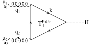
Figure 11: Two three-point functions connected by charge conjugation.

The two generic three-point functions depicted in Fig. 11 have the following expressions

$$T^{\mu_{1}\mu_{2}}_{1}(q_{1},q_{2}) = {1\over 4m_{t}}\int\frac{d^{4}k}{i\pi^{2}}{\rm Tr}\left(\frac{1}{k\kern-4.30554pt\hbox{/}-m_{t}}\gamma^{\mu_{1}}\frac{1}{k\kern-4.30554pt\hbox{/}+q\kern-4.30554pt\hbox{/}_{1}-m_{t}}\gamma^{\mu_{2}}\frac{1}{k\kern-4.30554pt\hbox{/}+q\kern-4.30554pt\hbox{/}_{1}+q\kern-4.30554pt\hbox{/}_{2}-m_{t}}\right),$$ (C.1)

$$T^{\mu_{1}\mu_{2}}_{2}(q_{1},q_{2}) = {1\over 4m_{t}}\int\frac{d^{4}k}{i\pi^{2}}{\rm Tr}\left(\frac{1}{k\kern-4.30554pt\hbox{/}-m_{t}}\gamma^{\mu_{2}}\frac{1}{k\kern-4.30554pt\hbox{/}+q\kern-4.30554pt\hbox{/}_{2}-m_{t}}\gamma^{\mu_{1}}\frac{1}{k\kern-4.30554pt\hbox{/}+q\kern-4.30554pt\hbox{/}_{1}+q\kern-4.30554pt\hbox{/}_{2}-m_{t}}\right),$$ (C.2)

where $q_{1}$ and $q_{2}$ are outgoing momenta and where we put an overall factor $1/(4m_{t})$ in front to delete a corresponding term coming from the trace over the top quark. Using the charge-conjugation matrix $C$

$$C\gamma_{\mu}C^{-1}=-\gamma^{T}_{\mu},$$ (C.3)

we can derive (Furry’s theorem)

$$T^{\mu_{1}\mu_{2}}_{1}\left(q_{1},q_{2}\right)=T^{\mu_{1}\mu_{2}}_{2}\left(q_{1},q_{2}\right)\equiv T^{\mu_{1}\mu_{2}}\left(q_{1},q_{2}\right).$$ (C.4)

In addition,

$$q_{1}^{\mu_{1}}T_{\mu_{1}\mu_{2}}(q_{1},q_{2})=q_{2}^{\mu_{2}}T_{\mu_{1}\mu_{2}}(q_{1},q_{2})=0$$ (C.5)

expresses the gauge invariance of the triangle graphs. The generic tensor structure satisfying Eq. (C.5) is then

$$T^{\mu_{1}\mu_{2}}\left(q_{1},q_{2}\right) = F_{T}\left(q_{1}^{2},q_{2}^{2},\left(q_{1}+q_{2}\right)^{2}\right)\,T_{T}^{\mu_{1}\mu_{2}}(q_{1},q_{2})+F_{L}\left(q_{1}^{2},q_{2}^{2},\left(q_{1}+q_{2}\right)^{2}\right)\,T_{L}^{\mu_{1}\mu_{2}}(q_{1},q_{2})$$ (C.6)

$$= F_{T}\,T_{T}^{\mu_{1}\mu_{2}}+F_{L}\,T_{L}^{\mu_{1}\mu_{2}},$$

where (dropping the dependence on external momenta $q_{1}$ and $q_{2}$, for ease of notation)

$$T_{T}^{\mu_{1}\mu_{2}} = q_{1}\cdot q_{2}\,g^{\mu_{1}\mu_{2}}-q_{1}^{\mu_{2}}\,q_{2}^{\mu_{1}}\;,$$ (C.7)

$$T_{L}^{\mu_{1}\mu_{2}} = q_{1}^{2}\,q_{2}^{2}\,g^{\mu_{1}\mu_{2}}-q_{1}^{2}\,q_{2}^{\mu_{1}}\,q_{2}^{\mu_{2}}-q_{2}^{2}\,q_{1}^{\mu_{1}}\,q_{1}^{\mu_{2}}+q_{1}\cdot q_{2}\,q_{1}^{\mu_{1}}q_{2}^{\mu_{2}}\;,$$ (C.8)

and

$$F_{L}(q_{1}^{2},q_{2}^{2},Q^{2}) = -{1\over 2\,{\rm det}{\cal Q}_{2}}\Bigg{\{}\left[2-{3\,q_{1}^{2}\,q_{2}\cdot Q\over{\rm det}{\cal Q}_{2}}\right]\Big{(}B_{0}\left(q_{1}\right)-B_{0}\left(Q\right)\Big{)}$$ (C.9)

$$\phantom{-{1\over 2\,{\rm det}{\cal Q}_{2}}}+\left[2-{3\,q_{2}^{2}\,q_{1}\cdot Q\over{\rm det}{\cal Q}_{2}}\right]\Big{(}B_{0}\left(q_{2}\right)-B_{0}\left(Q\right)\Big{)}$$

$$\phantom{-{1\over 2\,{\rm det}{\cal Q}_{2}}}-\left[4m_{t}^{2}+q_{1}^{2}+q_{2}^{2}+Q^{2}-{3\,q_{1}^{2}\,q_{2}^{2}\,Q^{2}\over{\rm det}{\cal Q}_{2}}\right]C_{0}\left(q_{1},q_{2}\right)+R\Bigg{\}}\;,\phantom{aaaaa}$$

$$F_{T}(q_{1}^{2},q_{2}^{2},Q^{2}) = -{1\over 2\,{\rm det}{\cal Q}_{2}}\bigg{\{}Q^{2}\Big{[}B_{0}\left(q_{1}\right)+B_{0}\left(q_{2}\right)-2B_{0}\left(Q\right)-2\,q_{1}\cdot q_{2}\,C_{0}\left(q_{1},q_{2}\right)\Big{]}$$ (C.10)

$$\phantom{-{1\over 2\,{\rm det}{\cal Q}_{2}}\bigg{\{}}+\left(q_{1}^{2}-q_{2}^{2}\right)\Big{(}B_{0}\left(q_{1}\right)-B_{0}\left(q_{2}\right)\Big{)}\bigg{\}}-q_{1}\cdot q_{2}\,F_{L}\;.$$

Here, the negative of $Q=q_{1}+q_{2}$ denotes the four-momentum of the Higgs boson, ${\rm det}{\cal Q}_{2}=q_{1}^{2}q_{2}^{2}-(q_{1}\cdot q_{2})^{2}$ is the Gram determinant, and the terms proportional to $R=-2$ are pole residues in $D=4$ dimensions, originating from contributions proportional to $(D-4)\,C_{24}(q_{1},q_{2})$ in the tensor reduction procedure. Please note that even though the $B_{0}$ functions are divergent in $\epsilon=(4-D)/2$, the form factors $F_{L}$ and $F_{T}$ are finite.

If one of the external momenta, for example $q_{1}$, is light-like (real photon or gluon), with polarization vector $\epsilon_{1}$, then

$$T_{L}^{\mu_{1}\mu_{2}}=q_{1}^{\mu_{1}}\left(q_{1}\cdot q_{2}\,q_{2}^{\mu_{2}}-q_{2}^{2}\,q_{1}^{\mu_{2}}\right)\quad{\rm if}\quad q_{1}^{2}=0,$$ (C.11)

and as a consequence of the orthogonality $q_{1}\cdot\epsilon_{1}=0$ we have

$$\epsilon_{1\mu_{1}}\,T_{L}^{\mu_{1}\mu_{2}}=0\;,$$ (C.12)

i.e. the form factor $F_{L}$ does not contribute when an on-shell gluon or photon is attached to the triangle graph.

The color structure of the sum of the two diagrams in Fig. 11 is straightforward. In fact, both the diagrams have the same color structure and we can write (see Eq. (C.4))

$${\rm Tr}\left(t^{a_{1}}t^{a_{2}}\right)T^{\mu_{1}\mu_{2}}_{1}\left(q_{1},q_{2}\right)+{\rm Tr}\left(t^{a_{2}}t^{a_{1}}\right)T^{\mu_{1}\mu_{2}}_{2}\left(q_{1},q_{2}\right)=\delta^{a_{1}a_{2}}\,T^{\mu_{1}\mu_{2}}\left(q_{1},q_{2}\right).$$ (C.13)

D Tensor and color structure of boxes

    

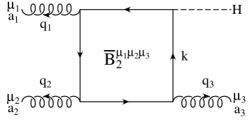
Figure 12: Two four-point functions connected by charge conjugation.

The two generic four-point functions connected by charge conjugation, depicted in Fig. 12, have the following expressions

$$\overline{B}^{\mu_{1}\mu_{2}\mu_{3}}_{1}(q_{1},q_{2},q_{3})\!\! = \!\!{1\over 4m_{t}}\int\frac{d^{4}k}{i\pi^{2}}\,{\rm Tr}\Bigg{(}\frac{1}{k\kern-4.30554pt\hbox{/}-m_{t}}\gamma^{\mu_{1}}\frac{1}{k\kern-4.30554pt\hbox{/}+q\kern-4.30554pt\hbox{/}_{1}-m_{t}}\gamma^{\mu_{2}}$$

$$\phantom{{1\over 4m_{t}}\int\frac{d^{4}k}{i\pi^{2}}\,{\rm Tr}\Bigg{(}}\times\frac{1}{k\kern-4.30554pt\hbox{/}+q\kern-4.30554pt\hbox{/}_{12}-m_{t}}\gamma^{\mu_{3}}\frac{1}{k\kern-4.30554pt\hbox{/}+q\kern-4.30554pt\hbox{/}_{123}-m_{t}}\Bigg{)},$$

$$\overline{B}^{\mu_{1}\mu_{2}\mu_{3}}_{2}(q_{1},q_{2},q_{3})\!\! =\!\! {1\over 4m_{t}}\int\frac{d^{4}k}{i\pi^{2}}\,{\rm Tr}\Bigg{(}\frac{1}{k\kern-4.30554pt\hbox{/}-m_{t}}\gamma^{\mu_{3}}\frac{1}{k\kern-4.30554pt\hbox{/}+q\kern-4.30554pt\hbox{/}_{3}-m_{t}}\gamma^{\mu_{2}}$$ (D.1)

$$\phantom{{1\over 4m_{t}}\int\frac{d^{4}k}{i\pi^{2}}\,{\rm Tr}\Bigg{(}}\times\frac{1}{k\kern-4.30554pt\hbox{/}+q\kern-4.30554pt\hbox{/}_{23}-m_{t}}\gamma^{\mu_{1}}\frac{1}{k\kern-4.30554pt\hbox{/}+q\kern-4.30554pt\hbox{/}_{123}-m_{t}}\Bigg{)},\phantom{aaaa}$$

where $q_{1},q_{2}$ and $q_{3}$ are the outgoing momenta, $q_{ij}=q_{i}+q_{j}$ and $q_{ijk}=q_{i}+q_{j}+q_{k}$. The overall factor $1/(4m_{t})$ cancels a corresponding term coming from the trace over the top quark. From charge conjugation we have

$$\overline{B}^{\mu_{1}\mu_{2}\mu_{3}}_{1}(q_{1},q_{2},q_{3})=-\overline{B}^{\mu_{1}\mu_{2}\mu_{3}}_{2}(q_{1},q_{2},q_{3})\equiv\overline{B}^{\mu_{1}\mu_{2}\mu_{3}}(q_{1},q_{2},q_{3})\;.$$ (D.2)

The color structure of the sum of the two diagrams depicted in Fig. 12 is

$${\rm Tr}\left(t^{a_{1}}t^{a_{2}}t^{a_{3}}\right)\overline{B}^{\mu_{1}\mu_{2}\mu_{3}}_{1}(q_{1},q_{2},q_{3})+{\rm Tr}\left(t^{a_{3}}t^{a_{2}}t^{a_{1}}\right)\overline{B}^{\mu_{1}\mu_{2}\mu_{3}}_{2}(q_{1},q_{2},q_{3})$$

$$\qquad\quad=\left[{\rm Tr}\left(t^{a_{1}}t^{a_{2}}t^{a_{3}}\right)-{\rm Tr}\left(t^{a_{3}}t^{a_{2}}t^{a_{1}}\right)\right]\overline{B}^{\mu_{1}\mu_{2}\mu_{3}}(q_{1},q_{2},q_{3})=\frac{i}{2}f^{a_{1}a_{2}a_{3}}\overline{B}^{\mu_{1}\mu_{2}\mu_{3}}(q_{1},q_{2},q_{3}),$$

where we have used the identity

$${\rm Tr}\left(t^{a_{1}}t^{a_{2}}t^{a_{3}}\right)=\frac{1}{4}\left(d^{a_{1}a_{2}a_{3}}+i\,f^{a_{1}a_{2}a_{3}}\right),$$ (D.4)

and the anti-symmetry of the structure constant $f^{a_{1}a_{2}a_{3}}$, together with the symmetry of $d^{a_{1}a_{2}a_{3}}$.

The sum over the six gluon permutations of boxes is then proportional to the single color factor $f^{a_{1}a_{2}a_{3}}$, and because of Bose symmetry of the gluons, the kinematic box factor

$$B^{\mu_{1}\mu_{2}\mu_{3}}(q_{1},q_{2},q_{3})=\overline{B}^{\mu_{1}\mu_{2}\mu_{3}}(q_{1},q_{2},q_{3})+\overline{B}^{\mu_{2}\mu_{3}\mu_{1}}(q_{2},q_{3},q_{1})+\overline{B}^{\mu_{3}\mu_{1}\mu_{2}}(q_{3},q_{1},q_{2})$$ (D.5)

is totally antisymmetric in the gluon indices $(q_{i},\mu_{i})$, $i=1,2,3$.

D.1 $qg\,\mbox{$\rightarrow$}\,qgH$ and $gg\,\mbox{$\rightarrow$}\,ggH$

The general structure of Eq. (D.5) can be further restricted for the processes we are investigating: $qg\,\mbox{$\rightarrow$}\,qgH$ and $gg\,\mbox{$\rightarrow$}\,ggH$. In fact, in both processes, two gluons of the box are on-shell, and the amplitude is contracted by the two corresponding polarization vectors $\epsilon_{i}$, while the third gluon is contracted with the conserved current $J_{21}^{\mu_{3}}$ (see Eq. (3.5)), in the $qg\,\mbox{$\rightarrow$}\,qgH$ process, and with the conserved current of the two on-shell gluons in the three-gluon vertex, in the $gg\,\mbox{$\rightarrow$}\,ggH$ case.

This gives rise to a few simplification in the structure of Eq. (D.5). In fact, a parity even, three-index tensor which depends on three independent momenta (here taken as the three outgoing gluon momenta $q_{i},\;i=1,2,3$) can be written in terms of 36 independent tensor structures, 9 of type $g^{\mu_{1}\mu_{2}}q_{i}^{\mu_{3}}$ and permutations, plus 27 tensors of type $q_{i}^{\mu_{1}}q_{j}^{\mu_{2}}q_{k}^{\mu_{3}}$. However, any terms proportional to $q_{1}^{\mu_{1}}$, $q_{2}^{\mu_{2}}$, or $q_{3}^{\mu_{3}}$ vanish by virtue of the transversity of the gluon polarization vectors $\epsilon_{i}^{\mu_{i}}$ and because the current on the vertex $\mu_{3}$ is conserved. This leaves us with 14 possible tensor structures, that can be further reduced to three once we impose the total antisymmetry in the gluon indices $(q_{i},\mu_{i})$

$$B^{\mu_{1}\mu_{2}\mu_{3}} = g^{\mu_{1}\mu_{2}}q_{1}^{\mu_{3}}\;B_{a}(q_{1},q_{2},q_{3})+g^{\mu_{2}\mu_{3}}q_{2}^{\mu_{1}}\;B_{a}(q_{2},q_{3},q_{1})+g^{\mu_{3}\mu_{1}}q_{3}^{\mu_{2}}\;B_{a}(q_{3},q_{1},q_{2})$$ (D.6)

$$- g^{\mu_{2}\mu_{1}}q_{2}^{\mu_{3}}\;B_{a}(q_{2},q_{1},q_{3})-g^{\mu_{1}\mu_{3}}q_{1}^{\mu_{2}}\;B_{a}(q_{1},q_{3},q_{2})-g^{\mu_{3}\mu_{2}}q_{3}^{\mu_{1}}\;B_{a}(q_{3},q_{2},q_{1})$$

$$+ q_{3}^{\mu_{1}}q_{3}^{\mu_{2}}q_{1}^{\mu_{3}}\;B_{b}(q_{1},q_{2},q_{3})+q_{2}^{\mu_{1}}q_{1}^{\mu_{2}}q_{1}^{\mu_{3}}\;B_{b}(q_{2},q_{3},q_{1})+q_{2}^{\mu_{1}}q_{3}^{\mu_{2}}q_{2}^{\mu_{3}}\;B_{b}(q_{3},q_{1},q_{2})$$

$$- q_{3}^{\mu_{1}}q_{3}^{\mu_{2}}q_{2}^{\mu_{3}}\;B_{b}(q_{2},q_{1},q_{3})-q_{2}^{\mu_{1}}q_{1}^{\mu_{2}}q_{2}^{\mu_{3}}\;B_{b}(q_{1},q_{3},q_{2})-q_{3}^{\mu_{1}}q_{1}^{\mu_{2}}q_{1}^{\mu_{3}}\;B_{b}(q_{3},q_{2},q_{1})$$

$$+ q_{2}^{\mu_{1}}q_{3}^{\mu_{2}}q_{1}^{\mu_{3}}\;B_{c}(q_{1},q_{2},q_{3})-q_{3}^{\mu_{1}}q_{1}^{\mu_{2}}q_{2}^{\mu_{3}}\;B_{c}(q_{2},q_{1},q_{3}).$$

Note that Bose symmetry implies that $B_{c}$ must be invariant under cyclic permutations of its arguments

$$B_{c}(q_{1},q_{2},q_{3})=B_{c}(q_{2},q_{3},q_{1})=B_{c}(q_{3},q_{1},q_{2}).$$ (D.7)

However, a convenient choice of gauge will remove the $B_{c}$ terms altogether, as shown in Sec. 3.2, using the polarization vectors defined in Eqs. (3.27) and (3.28).

The scalar functions appearing in Eq. (D.6) are given by

$$B_{a}(q_{1},q_{2},q_{3}) = {1\over 2}q_{2}\cdot q_{3}\Bigl{[}D_{0}(q_{1},q_{2},q_{3})+D_{0}(q_{2},q_{3},q_{1})+D_{0}(q_{3},q_{1},q_{2})\Bigr{]}$$ (D.8)

$${}-q_{1}\cdot q_{2}\Bigl{[}D_{13}(q_{2},q_{3},q_{1})+D_{12}(q_{3},q_{1},q_{2})-D_{13}(q_{3},q_{2},q_{1})\Bigr{]}-C_{0}(q_{1},q_{2}+q_{3})$$

$${}-4\Bigl{[}D_{313}(q_{2},q_{3},q_{1})+D_{312}(q_{3},q_{1},q_{2})-D_{313}(q_{3},q_{2},q_{1})\Bigr{]}\;,$$

$$B_{b}(q_{1},q_{2},q_{3}) = D_{13}(q_{1},q_{2},q_{3})+D_{12}(q_{2},q_{3},q_{1})-D_{13}(q_{2},q_{1},q_{3})$$ (D.9)

$${}+4\Bigl{[}D_{37}(q_{1},q_{2},q_{3})+D_{23}(q_{1},q_{2},q_{3})+D_{38}(q_{2},q_{3},q_{1})$$

$${}+D_{26}(q_{2},q_{3},q_{1})-D_{39}(q_{2},q_{1},q_{3})-D_{23}(q_{2},q_{1},q_{3})\Bigr{]}\;,$$

$$B_{c}(q_{1},q_{2},q_{3}) = -{1\over 2}\Bigl{[}D_{0}(q_{1},q_{2},q_{3})+D_{0}(q_{2},q_{3},q_{1})+D_{0}(q_{3},q_{1},q_{2})\Bigr{]}$$ (D.10)

$${}+4\Bigl{[}D_{26}(q_{1},q_{2},q_{3})+D_{26}(q_{2},q_{3},q_{1})+D_{26}(q_{3},q_{1},q_{2})$$

$${}+D_{310}(q_{1},q_{2},q_{3})+D_{310}(q_{2},q_{3},q_{1})+D_{310}(q_{3},q_{1},q_{2})\Bigr{]}\;.$$

Further simplifications appear in the evaluation of $qg\,\mbox{$\rightarrow$}\,qgH$ matrix elements. In fact, since the polarization vectors for the two on-shell gluons are either proportional to $x^{\mu}$ or $y^{\mu}$ (see Eqs. (3.27) and (3.28)), we only need the contractions $B_{xx\mu_{3}}=x_{\mu_{1}}x_{\mu_{2}}{B^{\mu_{1}\mu_{2}}}_{\mu_{3}}(q_{1},q_{2},q_{3})$, $B_{xy\mu_{3}}=x_{\mu_{1}}y_{\mu_{2}}{B^{\mu_{1}\mu_{2}}}_{\mu_{3}}$, etc. The $\mu_{3}$ index will be contracted with the fermion current $J_{21}^{\mu_{3}}$ (see Eq. (3.20)). Since $q_{1}$, $q_{2}$, $q_{3}$ and $y$ span Minkowski space, $J_{21}$ can be expanded as

$$J_{21}^{\mu}={1\over{\rm det}{\cal Q}_{3}}\Bigl{(}q_{1}\cdot J_{21}\;u^{\mu}+q_{2}\cdot J_{21}\;v^{\mu}+y\cdot J_{21}\;y^{\mu}\Bigr{)}\;,$$ (D.11)

where

$$u^{\mu} = q_{2}\cdot q_{3}\;x^{\mu}+{{\rm det}{\cal Q}_{3}\over q_{1}\cdot q_{2}}\,q_{2}^{\mu}\;,$$ (D.12)

$$v^{\mu} = q_{1}\cdot q_{3}\;x^{\mu}+{{\rm det}{\cal Q}_{3}\over q_{1}\cdot q_{2}}\,q_{1}^{\mu}\;,$$ (D.13)

and they satisfy the orthogonality relations

$$\begin{array}[]{llll}u\cdot q_{1}={\rm det}{\cal Q}_{3}\;,&u\cdot q_{2}=0\;,&u\cdot q_{3}=0\;,&u\cdot y=0\\ v\cdot q_{1}=0\;,&v\cdot q_{2}={\rm det}{\cal Q}_{3}\;,&v\cdot q_{3}=0\;,&v\cdot y=0\;,\end{array}$$ (D.14)

by virtue of the two on-shell conditions $q_{1}^{2}=0$ and $q_{2}^{2}=0$. Note that there is no $q_{3}$ contraction in Eq. (D.11), since $q_{3}\cdot J_{21}=0$ by current conservation.

The orthogonality of $y^{\mu}$ to all gluon momenta $q_{i},\;i=1,2,3$, implies that all contractions of $B^{\mu_{1}\mu_{2}\mu_{3}}$ with an odd number of $y$ will vanish. This leaves us with six non-zero contractions of the tensor box integrals, $B_{yyu}$, $B_{yyv}$, $B_{yxy}$, $B_{xyy}$, $B_{xxu}$ and $B_{xxv}$. Via the Bose symmetry of the tensor integral in Eq. (D.6), the first four and the last two are related by a permutation of gluon momenta:

$$B_{yyu} = \left({\rm det}{\cal Q}_{3}\right)^{2}\;B_{a}(q_{1},q_{2},q_{3})\;,$$ (D.15)

$$B_{yyv} = -\left({\rm det}{\cal Q}_{3}\right)^{2}\;B_{a}(q_{2},q_{1},q_{3})\;,$$ (D.16)

$$B_{yxy} = -{\left({\rm det}{\cal Q}_{3}\right)^{2}\over q_{1}\cdot q_{2}}\;B_{a}(q_{3},q_{1},q_{2})\;,$$ (D.17)

$$B_{xyy} = {\left({\rm det}{\cal Q}_{3}\right)^{2}\over q_{1}\cdot q_{2}}\;B_{a}(q_{3},q_{2},q_{1})\;,$$ (D.18)

$$B_{xxu} = \left({\rm det}{\cal Q}_{3}\right)^{2}\Bigg{\{}B_{a}\left(q_{1},q_{2},q_{3}\right)-{q_{2}\cdot q_{3}\over q_{1}\cdot q_{2}}\Big{[}B_{a}\left(q_{3},q_{1},q_{2}\right)-B_{a}\left(q_{3},q_{2},q_{1}\right)\Big{]}$$ (D.19)

$$\phantom{\left({\rm det}{\cal Q}_{3}\right)^{2}\Bigg{\{}}+{{\rm det}{\cal Q}_{3}\over(q_{1}\cdot q_{2})^{2}}B_{b}\left(q_{1},q_{2},q_{3}\right)\Bigg{\}}$$

$$= -{({\rm det}{\cal Q}_{3})^{2}\over q_{1}\cdot q_{2}}\Biggl{\{}(q_{1}\cdot q_{2})^{2}\Bigl{[}D_{13}(q_{2},q_{3},q_{1})+D_{12}(q_{3},q_{1},q_{2})-D_{13}(q_{3},q_{2},q_{1})\Bigr{]}$$

$${}-{1\over 2}q_{1}\cdot q_{2}\,q_{2}\cdot q_{3}\Bigl{[}D_{0}(q_{1},q_{2},q_{3})+D_{0}(q_{3},q_{1},q_{2})\Bigr{]}-q_{2}\cdot q_{3}\,q_{2}\cdot\left(q_{3}+{q_{1}\over 2}\right)D_{0}(q_{2},q_{3},q_{1})$$

$${}+4\,q_{1}\cdot q_{2}\Bigl{[}D_{313}(q_{2},q_{3},q_{1})+D_{312}(q_{3},q_{1},q_{2})-D_{313}(q_{3},q_{2},q_{1})\Bigr{]}$$

$${}+\Bigl{[}q_{2}\cdot q_{3}\,q_{3}\cdot(q_{1}-q_{2})-q_{3}^{2}\,q_{1}\cdot q_{2}\Bigr{]}\Bigl{[}D_{13}(q_{1},q_{2},q_{3})+D_{12}(q_{2},q_{3},q_{1})-D_{13}(q_{2},q_{1},q_{3})\Bigr{]}$$

$${}-4\,q_{2}\cdot q_{3}\Bigl{[}2\Bigl{(}D_{313}(q_{1},q_{2},q_{3})+D_{312}(q_{2},q_{3},q_{1})-D_{313}(q_{2},q_{1},q_{3})\Bigr{)}+D_{27}(q_{2},q_{3},q_{1})\Bigr{]}$$

$${}-4\,{{\rm det}{\cal Q}_{3}\over q_{1}\cdot q_{2}}\Bigl{[}D_{37}(q_{1},q_{2},q_{3})+D_{23}(q_{1},q_{2},q_{3})+D_{38}(q_{2},q_{3},q_{1})+D_{26}(q_{2},q_{3},q_{1})$$

$${}-D_{39}(q_{2},q_{1},q_{3})-D_{23}(q_{2},q_{1},q_{3})\Bigr{]}+q_{1}\cdot q_{2}\,C_{0}(q_{1},q_{2}+q_{3})\Biggr{\}}\;,$$

$$B_{xxv} = -({\rm det}{\cal Q}_{3})^{2}\Bigg{\{}B_{a}(q_{2},q_{1},q_{3})+{q_{1}\cdot q_{3}\over q_{1}\cdot q_{2}}\Big{[}B_{a}(q_{3},q_{1},q_{2})-B_{a}(q_{3},q_{2},q_{1})\Big{]}$$ (D.20)

$$\phantom{-({\rm det}{\cal Q}_{3})^{2}\Bigg{\{}}+{{\rm det}{\cal Q}_{3}\over(q_{1}\cdot q_{2})^{2}}B_{b}(q_{2},q_{1},q_{3})\Bigg{\}}$$

$$= -B_{xxu}(q_{1}\leftrightarrow q_{2})\;.$$

Note that in the replacement $B_{xxv}=-B_{xxu}(q_{1}\leftrightarrow q_{2})$, the Gram determinant, ${\rm det}{\cal Q}_{3}$, is to be treated as totally symmetric under interchange of gluon momenta $q_{1}$, $q_{2}$, and $q_{3}$.

E Tensor and color structure of pentagons

    

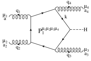
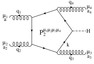
Figure 13: Two five-point functions connected by charge conjugation.

The two generic five-point functions connected by charge conjugation depicted in Fig. 13 have the following expression

$$P^{\mu_{1}\mu_{2}\mu_{3}\mu_{4}}_{1}(q_{1},q_{2},q_{3},q_{4})\!\! = \!\!{1\over 4m_{t}}\int\frac{d^{4}k}{i\pi^{2}}\,{\rm Tr}\Bigg{(}\frac{1}{k\kern-4.30554pt\hbox{/}-m_{t}}\gamma^{\mu_{4}}\frac{1}{k\kern-4.30554pt\hbox{/}+q\kern-4.30554pt\hbox{/}_{4}-m_{t}}\gamma^{\mu_{1}}\frac{1}{k\kern-4.30554pt\hbox{/}+q\kern-4.30554pt\hbox{/}_{14}-m_{t}}\gamma^{\mu_{2}}$$

$$\phantom{{1\over 4m_{t}}\int\frac{d^{4}k}{i\pi^{2}}\,{\rm Tr}\Bigg{(}}\times\frac{1}{k\kern-4.30554pt\hbox{/}+q\kern-4.30554pt\hbox{/}_{124}-m_{t}}\gamma^{\mu_{3}}\frac{1}{k\kern-4.30554pt\hbox{/}+q\kern-4.30554pt\hbox{/}_{1234}-m_{t}}\Bigg{)},$$

$$P^{\mu_{1}\mu_{2}\mu_{3}\mu_{4}}_{2}(q_{1},q_{2},q_{3},q_{4})\!\! = \!\!{1\over 4m_{t}}\int\frac{d^{4}k}{i\pi^{2}}\,{\rm Tr}\Bigg{(}\frac{1}{k\kern-4.30554pt\hbox{/}-m_{t}}\gamma^{\mu_{3}}\frac{1}{k\kern-4.30554pt\hbox{/}+q\kern-4.30554pt\hbox{/}_{3}-m_{t}}\gamma^{\mu_{2}}\frac{1}{k\kern-4.30554pt\hbox{/}+q\kern-4.30554pt\hbox{/}_{23}-m_{t}}\gamma^{\mu_{1}}$$ (E.1)

$$\phantom{{1\over 4m_{t}}\int\frac{d^{4}k}{i\pi^{2}}\,{\rm Tr}\Bigg{(}}\times\frac{1}{k\kern-4.30554pt\hbox{/}+q\kern-4.30554pt\hbox{/}_{123}-m_{t}}\gamma^{\mu_{4}}\frac{1}{k\kern-4.30554pt\hbox{/}+q\kern-4.30554pt\hbox{/}_{1234}-m_{t}}\Bigg{)},\phantom{aaaa}$$

where $q_{1},q_{2},q_{3}$ and $q_{4}$ are the outgoing momenta ($q_{ij}=q_{i}+q_{j}$ and similar ones for $q_{ijl}$ and $q_{ijln}$) and where we put an overall factor $1/(4m_{t})$ in front to delete a corresponding term coming from the trace over the top quark. From charge conjugation we have

$${P}^{\mu_{1}\mu_{2}\mu_{3}\mu_{4}}_{1}(q_{1},q_{2},q_{3},q_{4})={P}^{\mu_{1}\mu_{2}\mu_{3}\mu_{4}}_{2}(q_{1},q_{2},q_{3},q_{4})\equiv{P}^{\mu_{1}\mu_{2}\mu_{3}\mu_{4}}(q_{1},q_{2},q_{3},q_{4})\;.$$ (E.2)

Finally, the color structure of the sum of the two diagrams depicted in Fig. 13 is

$${\rm Tr}\left(t^{a_{1}}t^{a_{2}}t^{a_{3}}t^{a_{4}}\right){P}^{\mu_{1}\mu_{2}\mu_{3}\mu_{4}}_{1}(q_{1},q_{2},q_{3},q_{4})+{\rm Tr}\left(t^{a_{4}}t^{a_{3}}t^{a_{2}}t^{a_{1}}\right){P}^{\mu_{1}\mu_{2}\mu_{3}\mu_{4}}_{2}(q_{1},q_{2},q_{3},q_{4})$$

$$\qquad\qquad=\left[{\rm Tr}\left(t^{a_{1}}t^{a_{2}}t^{a_{3}}t^{a_{4}}\right)+{\rm Tr}\left(t^{a_{1}}t^{a_{4}}t^{a_{3}}t^{a_{2}}\right)\right]{P}^{\mu_{1}\mu_{2}\mu_{3}\mu_{4}}(q_{1},q_{2},q_{3},q_{4})\;.$$ (E.3)

Further details about the color structure of pentagons are given in Sec. 3.3.

References

- [1] G. L. Bayatian et al., CMS Technical Proposal, report CERN/LHCC/94-38x (1994); R. Kinnunen and D. Denegri, CMS NOTE 1997/057; R. Kinnunen and A. Nikitenko, CMS TN/97-106; R. Kinnunen and D. Denegri, hep-ph/9907291.
- [2] ATLAS Collaboration, ATLAS TDR, report CERN/LHCC/99-15 (1999).
- [3] D. Zeppenfeld, R. Kinnunen, A. Nikitenko and E. Richter-Was, Phys. Rev. D62, 013009 (2000) [hep-ph/0002036].
- [4] A. Djouadi, N. Spira and P. Zerwas, Phys. Lett. B264, 440 (1991); M. Spira, A. Djouadi, D. Graudenz and P.M. Zerwas, Nucl. Phys. B453, 17 (1995); S. Dawson, Nucl. Phys. B359, 283 (1991).
- [5] See e.g. LEP Electroweak Working Group, LEPEWWG Note 2001-01 (2001) and http://lepewwg.web.cern.ch/LEPEWWG/.
- [6] S. Catani, D. de Florian and M. Grazzini, JHEP 0105, 025 (2001) [hep-ph/0102227]; R. Harlander and W. Kilgore, Phys. Rev. D64, 013015 (2001) [hep-ph/0102241].
- [7] T. Han and S. Willenbrock, Phys. Lett. B273, 167 (1991).
- [8] V. Del Duca, W. Kilgore, C. Oleari, C. Schmidt and D. Zeppenfeld, preprint MADPH-01-1226 (2001) [hep-ph/0105129], Phys. Rev. Lett., in press.
- [9] K. Hagiwara and D. Zeppenfeld, Nucl. Phys. B313, 560 (1989).
- [10] P. Nogueira, J. Comput. Phys. 105, 279 (1993).
- [11] G. Passarino and M. Veltman, Nucl. Phys. B160, 151 (1979).
- [12] S. Dawson, R.P. Kauffman, Phys. Rev. Lett. 68, 2273 (1992); R.P. Kauffman, S.V. Desai, D. Risal, Phys. Rev. D55, 4005 (1997), Erratum-ibid. D58, 119901 (1998) [hep-ph/9610541].
- [13] H.L. Lai et al., Phys. Rev. D55, 1280, (1997) [hep-ph/9606399].
- [14] D. Rainwater, R. Szalapski and D. Zeppenfeld, Phys. Rev. D54 6680 (1996); D. Rainwater and D. Zeppenfeld, Phys. Rev. D60, 113004 (1999), Erratum-ibid. D61, 099901 (2000); D. Rainwater, PhD thesis, hep-ph/9908378; T. Plehn, D. Rainwater and D. Zeppenfeld, Phys. Rev. D61, 093005 (2000).
- [15] T. Plehn, D. Rainwater and D. Zeppenfeld, preprint MADPH-01-1229 (2001) [hep-ph/0105325].
- [16] G. ’t Hooft and M. Veltman, Nucl. Phys. B153, 365 (1979).
- [17] A. Denner, U. Nierste and R. Scharf, Nucl. Phys. B367, 637 (1991).
- [18] Z. Bern, L. Dixon and D. Kosower, Phys. Lett. B302, 299 (1993), Erratum-ibid. B318, 649 (1993) [hep-ph/9212308]; Z. Bern, L. Dixon and D. Kosower, Nucl. Phys. B412, 751 (1994) [hep-ph/9306240].