Quintessence in a Brane World

Abstract

We reanalyze a new quintessence scenario in a brane world model, assuming that a quintessence scalar field is confined in our 3-dimensional brane world. We study three typical quintessence models : (1) an inverse-power-law potential, (2) an exponential potential, and (3) kinetic-term quintessence ($k$-essence) model. With an inverse power law potential model ($V(\phi)=\mu^{\alpha+4}\phi^{-\alpha}$), we show that in the quadratic dominant stage, the density parameter of a scalar field $\Omega_{\phi}$ decreases as $a^{-4(\alpha-2)/(\alpha+2)}$ for $2<\alpha<6$, which is followed by the conventional quintessence scenario. This feature provides us wider initial conditions for a successful quintessence. In fact, even if the universe is initially in a scalar-field dominant, it eventually evolves into a radiation dominant era in the $\rho^{2}$-dominant stage.

Assuming an equipartition condition, we discuss constraints on parameters, resulting that $\alpha\geq 4$ is required. This constraint also restricts the value of the 5-dimensional Planck mass, e.g. $4\times 10^{-14}m_{4}\mbox{\raisebox{-4.30554pt}{$\stackrel{{\scriptstyle\textstyle<}}{{\textstyle\sim}}$}}m_{5}\mbox{\raisebox{-4.30554pt}{$\stackrel{{\scriptstyle\textstyle<}}{{\textstyle\sim}}$}}3\times 10^{-13}m_{4}$ for $\alpha=5$. For an exponential potential model $V=\mu^{4}\exp(-\lambda\phi/m_{4})$, we may not find a natural and successful quintessence scenario as it is. While, for a kinetic-term quintessence, we find a tracking solution even in $\rho^{2}$-dominant stage, rather than the $\Omega_{\phi}$-decreasing solution for an inverse-power-law potential. Then we do find a little advantage in a brane world. Only the density parameter increases more slowly in the $\rho^{2}$-dominant stage, which provides a wider initial condition for a successful quintessence.

]

I Introduction

Recent observation of the angular spectrum of the cosmic microwave background (CMB) in a wide range of $\ell$, besides the results for small $\ell$ obtained by COBE, suggests a flat universe[1]. By combining this result with the measurements of high-redshift supernovae[2], which predicts that the expansion of the universe is accelerating now, we are forced to recognize the existence of a cosmological constant, or a kind of dark energy, which value is almost the same order of magnitude as the present mass density of the universe. From the viewpoint of particle physics, however, it is quite difficult to explain such a tiny value by $14$ orders of magnitude smaller than the electroweak scale. The failure of theoretical explanations for the present value of the cosmological constant is known as the so-called ”Cosmological Constant Problem.” [3]

Since there is no plausible theoretical idea to explain such a small cosmological constant, it may be more plausible that such a tiny value is achieved through the dynamics of a fundamental field. This idea is called a decaying cosmological constant[4],[5]. Among such models, the so-called quintessence seems to be more promising. It shows an interesting property, i.e. a quintessence field follows a common evolutionary track just as an attractor in a wide range of the initial conditions, so that the cosmology is extremely insensitive to the initial conditions [6],[7], [8], [9]. Some of them (so-called ”tracker-fields”) may avoid the coincidence problem. According to a successful quintessence scenario, the energy of a scalar field tracks the radiation energy (or matter energy) for a rather long time in order not to affect the nucleosynthesis at the radiation dominant era, and the structure formation at the matter dominant era, and then becomes dominant just before the present time.

There seems to be, however, still a kind of fine-tuning problem for these models. Although the initial energy of a scalar field could be the same as that of radiation fluid, most contribution is from its kinetic energy. In the kinetic dominant case, the scalar field behaves as a massless field, which is equivalent to a stiff matter. Hence its energy density drops as $a^{-6}$ which is much faster than the radiation energy. Then the kinetic term drops in the radiation dominant universe until a tracking solution is found. This is why the density parameter of a scalar field decreases before reaching a tracking solution. Since we have to tune the mass scale of a potential for a successful quintessence, the potential term cannot be so large. Hence, an equipartition condition, which may be expected in the early stage of the universe, seems to be unlikely in such a model. Another unsatisfactory point is that if the universe starts in a scalar-field dominant condition, the radiation dominant universe is never recovered. Then we are not able to find the present universe. Some modified models within the conventional gravity theory have been proposed to solve such problems [10],[11].

As for the early stage of the universe, recently we have a new interesting idea, which is called brane cosmology. In a brane world scenario, our universe is embedded in higher dimensions and standard-model particles are confined to four-dimensional hypersurfaces (3-branes), while gravity is propagating in higher-dimensions (a bulk) [12] -[15]. Among them Randall-Sundrum’s second model is very interesting because it provides a new type of compactification of gravity. Assuming the 3-brane has positive tension and is embedded in 5-dimensional anti de-Sitter bulk spacetime, the conventional four-dimensional gravity theory is recovered, even though the extra dimension is not compact [14]. While, in a high energy region, gravity theory is very different from the four dimensional Einstein theory[16]. Many authors discussed the geometrical aspects and its dynamics (For a review, see, [17]), as well as cosmology [18], [19], [20].

The main modified point from conventional cosmology is the appearance of the quadratic term of energy-momentum and dark radiation. Since the quadratic term changes the dynamics of the universe in its early stage, we expect some improvement for a quintessence scenario. In [21], it is shown that the quadratic term indeed drastically changes the evolution of a scalar field with an inverse-power-law potential and then the density parameter of a scalar field decreases in time until conventional cosmology is recovered. This result helps to construct a more natural and successful quintessence scenario.

The purpose of the present paper is to present a full analysis of the previous letter, including a numerical analysis, and to study other types of quintessence models in the brane world scenario. In Sec.II, we present the basic equations assuming the Randall-Sundrum II model. We then study three typical quintessence models, an inverse-power-law potential model (in Sec.III), an exponential potential model (in Sec.IV), and a kinetic term quintessence ($k$-essence) model (in Sec.V). Sec. VI is devoted to the conclusions.

II BASIC EQUATIONS

We start with the Randall-Sundrum type II brane scenario[14], because the model is simple and concrete. It is, however, worthwhile noting that the present mechanism may also work in other types of brane world models, in which a quadratic term of energy-momentum tensor generically appears. In the brane world, all matter fields and forces except gravity are confined on the 3-brane in a higher-dimensional spacetime. As for gravity, in contrast to the other type of brane scenario, in the Randall-Sundrum type II model, the extra-dimension is not compactified, but gravity is confined in the brane, showing the Newtonian gravity in our world. Since the gravity is confined in the brane, it can be described by the intrinsic metric of the brane spacetime. By use of Israel’s thin shell formalism and assuming $Z_{2}$ symmetry, the gravitational equations on the 3-brane is given by

$${}^{(4)}G_{\mu\nu}=-^{(4)}\Lambda g_{\mu\nu}+\kappa_{4}^{2}T_{\mu\nu}+\kappa_{5}^{4}\pi_{\mu\nu}-E_{\mu\nu},$$ (1)

where ${}^{(4)}G_{\mu\nu}$ is the Einstein tensor with respect to the intrinsic metric $g_{\mu\nu}$, ${}^{(4)}\Lambda$ is the 4-dimensional cosmological constant, $T_{\mu\nu}$ represents the energy-momentum tensor of matter fields confined on the brane and $\pi_{\mu\nu}$ is quadratic in $T_{\mu\nu}$[16]. $E_{\mu\nu}$ is a part of the 5-dimensional Weyl tensor and carries some information about bulk geometry. $\kappa_{4}^{\;2}=8\pi G_{4}$ and $\kappa_{5}^{\;2}=8\pi G_{5}$ are 4-dimensional and 5-dimensional gravitational constants, respectively. In what follows, we use the 4-dimensional Planck mass $m_{4}\equiv\kappa_{4}^{~{}-1}=(2.4\times 10^{18}{\rm GeV})$ and the 5-dimensional Planck mass $m_{5}\equiv\kappa_{5}^{~{}-2/3}$, which could be much smaller than $m_{4}$. We also assume that ${}^{(4)}\Lambda$ vanishes.

Assuming the Friedmann-Robertson-Walker spacetime in our brane world, we find the Friedmann equations from Eq.(1) as

$$H^{2}+{k\over a^{2}} = \frac{1}{3m_{4}^{\;2}}\rho+\frac{1}{36m_{5}^{\;6}}\rho^{2}+\frac{{\cal C}}{a^{4}}$$ (2)

$$\dot{H}-{k\over a^{2}} = -\frac{1}{2m_{4}^{\;2}}\left(P+\rho\right)-\frac{1}{12m_{5}^{\;6}}\rho\left(P+\rho\right)-\frac{2{\cal C}}{a^{4}}$$ (3)

where $a$ is a scale factor of the Universe, $H=\dot{a}/a$ is its Hubble parameter, $k$ is a curvature constant, $P$ and $\rho$ are the total pressure and total energy density of matter fields. ${\cal C}$ is a constant, which describes ”dark” radiation coming from $E_{\mu\nu}$ [18]. In what follows, we consider only the flat Friedmann model ($k=0$) for simplicity.

As for matter fields on the brane, we consider a scalar field $\phi$ as well as the conventional radiation and matter fluids, i.e. $\rho=\rho_{\phi}+\rho_{\rm r}+\rho_{\rm m}$, where $\rho_{\phi},\rho_{\rm r}$ and $\rho_{\rm m}$ are the energy densities of scalar field $\phi$, of radiation fluid and of matter one, respectively. Although we can consider a 5-dimensional scalar field living in the bulk[22], we shall focus only on a 4-dimensional scalar field confined on the brane. The origin of such a scalar field might be a condensation of some fermions confined on the brane.

Since the energy of each field on the brane is conserved in the present model, we find the dynamical equation for such a 4-dimensional scalar field as a conventional one, i.e.

$$\ddot{\phi}+3H\dot{\phi}+\frac{dV}{d\phi}=0,$$ (4)

where $V$ is a potential of the scalar field. The energy density of the scalar field is

$$\rho_{\phi}=\frac{1}{2}\dot{\phi}^{2}+V(\phi),$$ (5)

and for the radiation and matter fluids, we have

$$\dot{\rho_{\rm r}}+4H\rho_{\rm r} = 0,$$ (6)

$$\dot{\rho_{\rm m}}+3H\rho_{\rm m} = 0.$$ (7)

As the Universe expands, the energy density decreases. This means that the quadratic term was very important in the early stage of the Universe. Comparing two terms (the conventional energy density term and the quadratic one), we find that the quadratic term dominates when

$$\rho>\rho_{c}\equiv 12m_{5}^{~{}6}/m_{4}^{~{}2}.$$ (8)

When the quadratic term is dominant, the expansion law of the Universe is modified. For example, in the radiation dominant era, i.e. $\rho_{\rm r}\gg\rho_{\rm m},\rho_{\phi}$, the Universe expands as $a\propto t^{1/4}$, in contrast with $t^{1/2}$ in the conventional radiation dominant era.

Since we are interested in a quintessence scenario and then the dynamical behavior of a scalar field, we shall calculate the density parameter of the scalar field, which is a ratio of the energy density of the scalar field to that of total energy density ($\Omega_{\phi}$). Ignoring dark radiation, we find

$$\dot{\Omega_{\phi}}=\frac{H\rho_{\rm r}}{\rho^{2}}\left(4V(\phi)-\dot{\phi}^{2}\right).$$ (9)

When the quadratic term dominates in the early stage, the Hubble expansion rate decreases. As a result, the friction term in Eq. (4) becomes small and then the dynamics of the scalar field will drastically change from the conventional one even for the same potential. It is easily expected that a kinetic term will play a more important role in the energy density of a scalar field. Consequently, if $\dot{\phi}^{2}>4V(\phi)$, the density parameter of a scalar field will decrease in time. In particular, this feature may be very important in a quintessence scenario, because most quintessence models assume very small potential energy, initially, for a successful scenario. We will show that this interesting feature of a scalar field is found in some quintessence models and the initial conditions for a successful scenario become much wider.

In the following sections, assuming that a quintessence field exists in a quadratic term dominant era, we investigate the dynamical behavior of a quintessence scalar field and search for a natural and successful quintessence scenario. We study three types of quintessence fields: models with an inverse power law potential, with an exponential potential and a kinetically driven model.

III Inverse power law potential

In this section, we investigate a model with an inverse power law potential[6],[7], i.e.

$$V\left(\phi\right)=\mu^{\alpha+4}\phi^{-\alpha},$$ (10)

where $\mu$ is a typical mass scale of the potential, which is not fixed here. Although this potential is not renormalizable, it may appear as an effective potential for a kind of fermion condensation in a supersymmetric QCD model[23]. The $SU(N_{c})$ gauge symmetry is broken by a pair condensation of $N_{f}$-flavor quarks, and the effective potential for a fermion condensate field $\phi$ is given by (10) with $\alpha=2(N_{c}+N_{f})/(N_{c}-N_{f})$.

The quintessence scenario with this potential has been well studied in the conventional universe[8]. We therefore turn our attention mainly to the quadratic term ($\rho^{2}$) dominant stage. Although some analytic solutions are already given in Ref.[21], we first summarize those and then show numerical analysis. We then discuss a natural quintessence scenario by this model and give some constraints for unknown parameters such as $m_{5}$ .

A Analytic solutions in $\rho^{2}$-dominant stage.

In the conventional universe, matter energy density is negligibly small in comparison with radiation energy density in the early stage of the universe. Then we know that it is also the case in the $\rho^{2}$-dominant stage. Hence we consider only radiation fluid and a scalar field $\phi$. As for the initial conditions, we have two possible cases: one is the radiation dominant case and the other is the $\phi$-dominant one. We discuss these separately.

$\left(1\right)$ radiation dominant initial conditions

In this case, the scale factor expands as $a\propto t^{1/4}$ and the equation for the scalar field (4) is now

$$\ddot{\phi}+\frac{3}{4t}\dot{\phi}-\alpha\mu^{\alpha+4}\phi^{-\alpha-1}=0.$$ (11)

We find an analytic solution for $\alpha<6$[21], that is

$$\phi = \phi_{0}\left({t\over t_{0}}\right)^{\frac{2}{\alpha+2}},$$ (13)

$${\rm with}~{}~{}~{}\phi_{0}^{\alpha+2}={2\alpha(\alpha+2)^{2}\over 6-\alpha}\mu^{\alpha+4}t_{0}^{2}$$

where $t_{0}$ and $\phi_{0}$ are integration constants. The constraint (13) requires $\alpha<6$. The energy density of the scalar field evolves as

$$\rho_{\phi} = {3\alpha(\alpha+2)\over 6-\alpha}V_{0}\left({t\over t_{0}}\right)^{-\frac{2\alpha}{\alpha+2}}$$ (14)

$$= {3\alpha(\alpha+2)\over 6-\alpha}V_{0}\left({a\over a_{0}}\right)^{-\frac{8\alpha}{\alpha+2}},$$ (15)

where $V_{0}=V(\phi_{0})$ and $a_{0}=a(t_{0})$. As for the density parameter $\Omega_{\phi}$, we find that

$$\Omega_{\phi}={\rho_{\phi}\over\rho_{\rm r}+\rho_{\phi}}\approx{\rho_{\phi}\over\rho_{\rm r}}=\Omega_{\phi}^{(0)}\left({a\over a_{0}}\right)^{\frac{4(2-\alpha)}{\alpha+2}},$$ (16)

where $\Omega_{\phi}^{(0)}={3\alpha(\alpha+2)\over 6-\alpha}V_{0}/\rho_{\rm r}(t_{0})$ because $\rho_{\rm r}\propto a^{-4}$.

If $\alpha>2$, just contrary to the tracking solution, the scalar field energy decreases faster than that of the radiation. This result is confirmed by Eq.(9) with the fact that the kinetic energy of a scalar field $\rho_{\phi}^{~{}(K)}=\dot{\phi}^{2}/2$ turns out to be larger than $4V$ as $\rho_{\phi}^{~{}(K)}/(4V)=2\alpha/(6-\alpha)$.

If $\alpha=2$, the scalar field energy drops at the same rate as that of the radiation until the conventional universe is recovered. This is the so-called ”scaling” solution. If $\alpha<2$, the scalar field energy decreases slower than the radiation energy, and eventually the scalar field dominates the radiation.

What happens for $\alpha\geq 6$ ? Since there is no asymptotic solution for which a kinetic term balances with a potential term, we expect that a kinetic term dominant solution is obtained asymptotically. It is easy to show that a potential dominant (or slow rolling) condition is not preserved asymptotically.

Assuming that a kinetic term is dominant, Eq. (11) is now

$$\ddot{\phi}+\frac{3}{4t}\dot{\phi}=0,$$ (17)

finding an asymptotic solution

$$\phi\propto t^{\frac{1}{4}}.$$ (18)

With this solution, we find that

$$\rho_{\phi}^{~{}(K)} = {1\over 2}\dot{\phi}^{2}\propto t^{-3/2}$$ (19)

$$\rho_{\phi}^{~{}(P)} = \mu^{\alpha+4}\phi^{-\alpha}\propto t^{-\alpha/4},$$ (20)

where $\rho_{\phi}^{~{}(K)}$ and $\rho_{\phi}^{~{}(P)}$ denote the kinetic and the potential terms of the energy density of a scalar field, respectively. Hence, if $\alpha\geq 6$, kinetic term dominance is guaranteed. This is also confirmed by numerical calculation.

$\left(2\right)$ $\phi$-dominant initial conditions

If a scalar field initially dominates radiation, what we will find in the dynamics of the scalar field? In the conventional universe, once a quintessence field dominates, radiation dominance will not be obtained. In the present model, however, a radiation dominant era is recovered as we will see.

Assuming the scalar field dominance, we find the Friedmann equation (2) as

$$H=\frac{1}{6m_{5}^{\;3}}\left[\frac{1}{2}\dot{\phi}^{2}+\mu^{\alpha+4}\phi^{-\alpha}\right],$$ (21)

while the equation for the scalar field (4) is

$$\ddot{\phi}+3H\dot{\phi}-\alpha\mu^{\alpha+4}\phi^{-\alpha-1}=0.$$ (22)

Inserting Eq. (21) into Eq. (22), we find a second order differential equation for $\phi$. The asymptotic behavior of the solution can be classified into three cases: (a) slow rolling (a potential term dominant) solution $\left(\alpha<2\right)$, (b) a solution in which the potential term balances with the kinetic term $\left(\alpha=2\right)$, and (c) a kinetic term dominant solution $\left(\alpha>2\right)$.

First, assuming a slow rolling condition $(\dot{\phi}^{2}\ll V$ and $|\ddot{\phi}|\ll H|\dot{\phi}|,|V^{\prime}|)$, Eqs. (21) and (22) are

$$H = \frac{1}{6m_{5}^{\;3}}\mu^{\alpha+4}\phi^{-\alpha},$$ (23)

$$3H\dot{\phi} - \alpha\mu^{\alpha+4}\phi^{-\alpha-1}=0.$$ (24)

From Eqs. (23) and (24), we obtain $\phi\dot{\phi}=2\alpha m_{5}^{\;3}$, finding an analytic solution

$$\frac{\phi}{m_{5}}=2\left(\alpha m_{5}\right)^{1/2}\left(t-t_{0}\right)^{1/2},$$ (25)

where $t_{0}$ is an integration constant. With this solution, we have $\dot{\phi}^{2}\propto t^{-1}$ and $V\propto t^{-\alpha/2}$. In order to guarantee the slow-rolling conditions, we have to require $\alpha<2$. In this case, the Universe expands as

$$a=a_{0}\exp\left\{\left[H_{0}\left(t-t_{0}\right)\right]^{(2-\alpha)/2}\right\},$$ (26)

where a constant $H_{0}$ is given by

$$\left({H_{0}\over m_{5}}\right)^{(2-\alpha)/2}={1\over\left[3\left(2-\alpha\right)\left(2\sqrt{\alpha}\right)^{\alpha}\right]}\left({\mu\over m_{5}}\right)^{\alpha+4}.$$ (27)

Note that this solution describes an inflationary evolution, whose expansion is weaker than the conventional exponential inflation, but stronger than the power-law type. Although this solution does not play into anything with a quintessence scenario, it may be interesting to discuss a spectrum of density perturbations for such an inflationary scenario. The results will be published elsewhere.

Secondly, we assume a kinetic term dominance. Eqs. (21) and (22) are now

$$H = \frac{1}{12m_{5}^{\;3}}\dot{\phi}^{2},$$ (28)

$$\ddot{\phi} + 3H\dot{\phi}=0.$$ (29)

Combining Eqs. (28) and (29), we have $\ddot{\phi}=-(1/4m_{5}^{\;3})\dot{\phi}^{3}$, finding a solution as

$$\frac{\phi}{m_{5}}=\pm 2\sqrt{2}m_{5}^{1/2}\left(t-t_{0}\right)^{1/2}+\frac{\phi_{0}}{m_{5}},$$ (30)

where $t_{0}$ and $\phi_{0}$ are integration constants. For the solution with $+$ sign, the potential term decreases as $V\propto t^{-\alpha/2}$, while the kinetic term drops as $\dot{\phi}^{2}\propto t^{-1}$. Hence, if $\alpha>2$, the kinetic term dominance condition is preserved. From Eq. (28), we find that the Universe expands as

$$a=a_{0}(t/t_{0})^{1/6},$$ (31)

and then the energy density of the scalar field decreases as $\rho_{\phi}\propto t^{-1}\propto a^{-6}$, while $\rho_{r}\propto a^{-4}$. Therefore, with this solution, the scalar field energy decreases faster than that of radiation, and eventually radiation dominance will be reached.

For the solution (30) with $-$ sign, the scalar field evolves into 0 as $t$ approaches a critical value $t_{\rm cr}$ large, climbing the potential as $V\rightarrow\infty$. However, before reaching this critical point, the potential becomes dominant, and then the assumption of a kinetic dominance is no longer valid in this limit. With the previous analysis for the potential dominance, we expect that this solution will also reach to radiation dominant stage. This is confirmed by numerical calculations. As a conclusion, the asymptotic behavior for the case with $\alpha>2$ is described by kinetic term dominance of the scalar field, followed eventually by radiation dominance.

For the remaining case of $\alpha=2$, we find an analytic solution[21], which is a power law expansion of the Universe

$$a=a_{0}(t/t_{0})^{p},$$ (32)

with

$$p=\frac{1}{6}\left[1+\frac{1}{8}\left(\frac{\mu}{m_{5}}\right)^{6}\right].$$ (33)

and

$$\phi=2\sqrt{2}m_{5}^{3/2}t^{1/2}.$$ (34)

The scalar field energy density evolves as

$$\rho_{\phi}\propto t^{-1}\propto a^{-1/p}.$$ (35)

If $\mu>40^{1/6}m_{5}\approx 1.85m_{5}$, $p>1$, that is, we find a power-law inflationary solution. The power-law inflation is, however, nothing to do with quintessence, although it may be interesting in the early universe. If $\mu<4^{1/6}m_{5}\approx 1.26m_{5}$, $p<1/4$, and then the scalar field energy decreases faster than that of radiation.

$\alpha$	$\mu$	initial	fate	feature
$\alpha<2$	any values	S	S	inflation
		R
	$\mu/m_{5}\geq 40^{1/6}$		S	PL inflation
$\alpha=2$	$~{}4^{1/6}<\mu/m_{5}<40^{1/6}~{}$	S		D.E
	$\mu/m_{5}<4^{1/6}$		R	scaling
	any values	R
$2<\alpha<6$	any values	S	R	const
		R
$\alpha\geq 6$	any values	S	R	kinetic
		R

TABLE I.: The fate of a scalar field for each initial condition, where S and R denote scalar field dominance ($\rho_{\phi}\gg\rho_{\rm r}$) and radiation dominance ($\rho_{\rm r}\gg\rho_{\phi}$), respectively. The “scaling” means the scaling solution ($\Omega_{\phi}$ =constant). The asymptotic behavior of $\rho_{\phi}^{(P)}/\rho_{\phi}^{(K)}={\rm constant}$ is described by “const”, while the kinetic dominance of $\rho_{\phi}^{(K)}\gg\rho_{\phi}^{(P)}$ is denoted by “kinetic”. “PL” is power-law. “DE” is decelerating power-law expansion.

Hence radiation dominance will eventually be obtained. For $4^{1/6}m_{5}<\mu<40^{1/6}m_{5}$, we can easily show that this solution is a global attractor and the ratio of radiation energy to that of the scalar field remains constant[24].

We summarize the obtained analytic solutions and its fate in Table 1.

B Numerical analysis in $\rho^{2}$-dominant stage

Now we study the dynamical property of the scalar field numerically and show that the above analytic solutions are really attractors. The systematic analysis of the dynamical properties of the scalar field in the quadratic dominant stage will be given elsewhere[24]. Here we consider only the case of $2<\alpha<6$ because we are interested in quintessence.

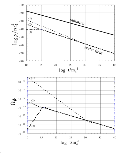
FIG. 1.: (Top) The time evolution of $\rho_{\rm r}$ and $\rho_{\phi}$ starting from a radiation dominant initial condition. We set $m_{5}=2.15\times 10^{-3}m_{4}$, and $\mu=1.0\times 10^{-8}m_{4}$. As for initial conditions, we set $\rho_{\rm r}=1.0\times 10^{-18}m_{4}^{\;4}$, $\rho_{\phi}^{~{}(K)}=0$ and $\rho_{\phi}^{~{}(P)}=1.0\times 10^{-29}m_{4}^{\;4},1.0\times 10^{-35}m_{4}^{\;4},$ and $1.0\times 10^{-41}m_{4}^{\;4}$ for (1), (2), and (3), respectively. If $\rho_{\phi}$ is initially greater than the value of the attractor solution (case (1)), the kinetic term soon dominates and eventually the attractor solution is reached. If $\rho_{\phi}$ is initially less than the attractor’s value (case (3)), the potential term dominates until the solution reaches the attractor. Thus, for a wide range of initial conditions ((1) $\sim$ (3)), $\rho_{\phi}$ reaches that of the attractor solution. (Bottom) Corresponding density parameter of the scalar field ($\Omega_{\phi}$) decreases after the attractor solution is reached.

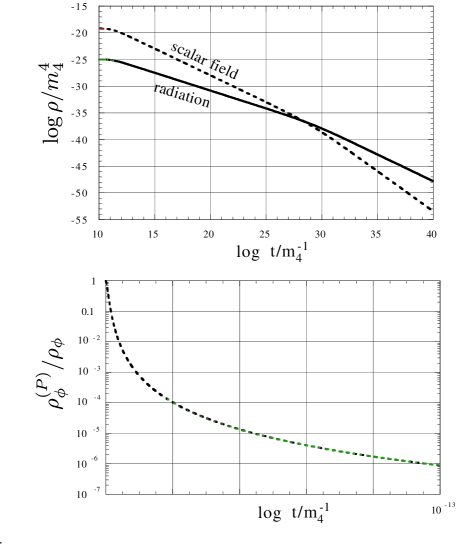
FIG. 2.: (Top) The time evolution of $\rho_{\rm r}$ and $\rho_{\phi}$ from the scalar-field dominant initial condition. The kinetic term soon dominates the energy density of the scalar field, and radiation dominance is eventually reached. As for initial conditions, we set $\rho_{\rm r}=1.0\times 10^{-25}m_{4}^{\;4}$, $\rho_{\phi}^{~{}(K)}=9.35\times 10^{-20}m_{4}^{\;4}$, $\rho_{\phi}^{~{}(P)}=1.0\times 10^{-17}m_{4}^{\;4},$ (Bottom) The time evolution of the ratio of the potential term of the energy density of a scalar field to the total total energy density of the scalar field. This suggests that the kinetic term dominates the potential term soon. We set $m_{5}=2.15\times 10^{-3}m_{4}$, and $\mu=1.0\times 10^{-8}m_{4}$.

First, we show that the solution (13) is a unique attractor for plausible initial conditions. We depict the evolution of $\rho_{\rm r}$ and $\rho_{\phi}$ for various initial conditions in Figs.1 and 2 for $\alpha=3$. The figures in Fig.1 show that for a wide range of initial conditions, the energy density of the scalar field approaches that of the attractor solution (13). We also find that even starting from scalar field dominance, the universe eventually evolves into the radiation dominant stage (see Fig. 2). In fact, the kinetic term of a scalar field always turns out to be dominant even if we start with a potential dominance. Since $\rho_{\phi}\propto a^{-6}$ in the case of the kinetic term dominance and $\rho_{r}\propto a^{-4}$, radiation energy eventually overcomes that of the scalar field and the Universe evolves into a radiation dominant era. As a result, the attractor solution is always reached for any initial conditions. We find similar results for any value of $\alpha$ in $2<\alpha<6$. We may conclude that the solution (13) is a unique attractor in the present dynamical system.

Once the attractor is reached, the scalar field energy decreases faster than that of radiation, which is a most interesting feature in the brane quintessence scenario. It is worthwhile noting that this potential in the conventional cosmology without the quadratic term, the quintessence scenario does not work if the scalar field energy initially dominates that of radiation[8]. Next, we shall discuss a more natural quintessence scenario in the brane world.

C Quintessence scenario

Now we are ready to discuss a quintessence scenario in the brane world[21]. We assume $2<\alpha<6$. Using two attractor solutions (one in the $\rho^{2}$-dominant stage and the other in the conventional universe), we show a successful and natural scenario. Since the quintessence solution in the conventional universe model is an attractor, our solution should also recover the same trajectory after the quadratic term decreases to be very small. We have confirmed this numerically. The main difference is that we can include not only radiation dominant initial conditions but also scalar-field dominant initial conditions for a successful scenario. In the numerical analysis, to evaluate the present value of the density parameter of a scalar field, we include the matter fluid as well as radiation and scalar field.

$\left(1\right)$ a scenario

First, we shall overview a quintessence scenario using attractor solutions[21]. We introduce $t_{s}$ (the cosmic time when the attractor solution in $\rho^{2}$ dominant stage is reached), $t_{c}$ (when the $\rho^{2}$-term drops just below the conventional density term), $t_{\rm NS}$(nucleosynthesis), $t_{\rm eq}$(when radiation energy density becomes equal to matter density), $t_{\rm dec}$(the decoupling time) and $t_{0}$ (the present time). If we approximate the evolution of the Universe by the attractor solutions in each stage, we find the analytic solution for the scalar field as follows. Normalizing the variables by 4-dimensional Planck mass scale $m_{4}$, we find that the energy density $\rho_{\phi}$ in each stage is described very simply as

$$\frac{\rho_{\phi}}{m_{4}^{4}}=\left[\alpha(\alpha+2)^{2}\right]^{-{\alpha\over\alpha+2}}F(\alpha)\left({\mu\over m_{4}}\right)^{2(\alpha+4)\over(\alpha+2)}(m_{4}t)^{-\frac{2\alpha}{\alpha+2}},$$ (36)

where $F(\alpha)$ is a dimensionless constant defined only by $\alpha$. In the $\rho^{2}$-dominant stage,

$$F(\alpha)=(\alpha+2)\left({2\over 6-\alpha}\right)^{2\over\alpha+2}.$$ (37)

and in the conventional universe,

$$F(\alpha) = (5\alpha+12)\left[2(\alpha+6)\right]^{-{2\over\alpha+2}}$$ (39)

$$~{}~{}~{}~{}~{}~{}~{}~{}~{}~{}{\rm(radiation~{}dominant~{}era)}$$

$$= 2^{3\alpha+2\over\alpha+2}(\alpha+2)(\alpha+4)^{-{2\over\alpha+2}}$$ (41)

$$~{}~{}~{}~{}~{}{\rm(matter~{}dominant~{}era)}.$$

Since the attractor solutions are independent, when the Universe shifts from one attractor solution to the other one, we expect a discrepancy in the energy density. However, since the difference in $\rho_{\phi}$ in each stage appears only in the factor $F(\alpha)$, the discrepancy between two attractor solutions is given by $\alpha$. We can easily check that the ratio of $F$ at the $\rho^{2}$-dominance to that in the conventional radiation dominance is about 0.5 to 1 unless $\alpha\approx 6$. Note that the ratio of radiation dominant case to matter dominant case is about 0.8 for any values of $\alpha$. Hence, when $t=t_{c}$, there is a little discrepancy between the scalar field energy densities estimated by two attractor solutions.

Although the energy density of a scalar field changes quite similarly in any stages, the radiation energy shows a big difference between $\rho^{2}$-dominant stage and the conventional universe. In fact, the radiation density decreases as $a^{-4}$, but the scale factor changes as $a\propto t^{1/4}$ in the $\rho^{2}$-dominant stage in contrast with $a\propto t^{1/2}$ in the conventional radiation dominant era. Therefore, when we discuss the density parameter of a scalar field $\Omega_{\phi}\sim\rho_{\phi}/\rho_{\rm r}$, its behavior in the $\rho^{2}$-dominant stage is completely different from that in the conventional universe.

$$\Omega_{\phi} \propto t^{(2-\alpha)/(2+\alpha)}\sim a^{(2-\alpha)/(2+\alpha)}~{}~{}~{}(\rho^{2}{\rm-dominant})$$ (42)

$$\propto t^{4/(2+\alpha)}\sim a^{8/(2+\alpha)}~{}~{}~{}({\rm radiation~{}dominant})$$ (43)

$$\propto t^{4/(2+\alpha)}\sim a^{6/(2+\alpha)}~{}~{}~{}({\rm matter~{}dominant})$$ (44)

Since the radiation energy must be continuous, if we ignore the above small discrepancies at $t_{c}$ and $t_{\rm eq}$, we can estimate the density parameter $\Omega_{\phi}$ as

$$\Omega_{\phi} = \Omega_{\phi}^{~{}(s)}\times\left({a_{c}\over a_{s}}\right)^{-{\alpha-2\over 2\alpha+2}}\times\left({a_{\rm eq}\over a_{c}}\right)^{8\over\alpha+2}\times\left({a_{0}\over a_{\rm eq}}\right)^{6\over\alpha+2}$$ (45)

$$= \Omega_{\phi}^{~{}(s)}\times\left({T_{s}\over T_{c}}\right)^{-{\alpha-2\over 2\alpha+2}}\times\left({T_{c}\over T_{\rm eq}}\right)^{8\over\alpha+2}\times\left({T_{\rm eq}\over T_{0}}\right)^{6\over\alpha+2},$$ (46)

where $\Omega_{\phi}^{~{}(s)}$ is the density parameter when the attractor solution is reached. For a successful quintessence scenario, we require that the present value of the density parameter of the scalar field is $\Omega_{\phi}\sim 0.7$.

Before finding a constraint, it may be useful to confirm the above analysis by numerical study. This is because with the above analytic attractor solutions, we cannot properly treat the transition between $\rho^{2}$-dominant stage and the conventional universe. We show one numerical result for $\alpha=5$. We set $\mu=6.0\times 10^{-14}m_{4}$ , $m_{5}=6.0\times 10^{-14}m_{4}$for a successful quintessence.

As initial conditions at $a_{s}=1$, we have chosen the attractor solution Eq.(15) in the $\rho^{2}$-dominant stage, and solve the basic equations (2),(4), (6) and (7) including radiation and matter fluids. In Fig.3, we depict the energy densities of a scalar field, radiation and matter in terms of a scale factor $a$. It turns out, as we expected, the discrepancy at $a_{c}$ is very small and the evolution approximately follows the attractors in each stage (attractor solutions as references).

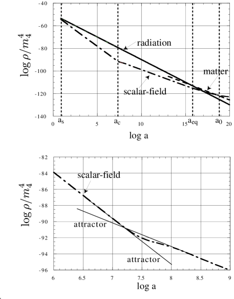
FIG. 3.: (Top) The evolution of the energy densities in terms of a scale factor. We set $\mu=6.0\times 10^{-14}m_{4}$, and $m_{5}=6.0\times 10^{-14}m_{4}$. As for the initial conditions, we set $\rho_{\phi}^{~{}(K)}=3.82\times 10^{-55}m_{4}^{\;4},\rho_{\phi}^{~{}(P)}=2.50\times 10^{-56}m_{4}^{\;4},$ and $\rho_{\rm r}=3.78\times 10^{-54}m_{4}^{\;4}$. The matter fluid is also included to find the present matter dominant universe as $\rho_{\rm m}=5.43\times 10^{-69}m_{4}^{\;4}$. The amount of matter fluid is chosen in order to find the present universe.
(Bottom) The enlargement of the top figure around the transition era from $\rho^{2}$-dominant stage to the conventional universe. The thin solid lines are attractor solutions both in $\rho^{2}$-dominant stage and in the conventional universe.

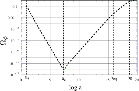
FIG. 4.: Time evolution of the density parameter of a scalar field for the same model in Fig.3.

From Fig.3, we find that $\rho_{\phi}\sim 10^{-90}m_{4}^{\;4}$ at $t_{c}$, $\sim 10^{-112}m_{4}^{\;4}$ at decoupling time, and $\sim 10^{-120}m_{4}^{\;4}$ at present (see Fig.3). These small values guarantee a successful quintessence. The conventional quintessence scenario (a tracking solution) is really recovered when the quadratic energy density becomes small enough. We also show the evolution of the density parameter of the scalar field in Fig.4

$\left(2\right)$ constraints to the extra-dimension

We discuss constraints for a natural and successful quintessence. We consider three constraints: nucleosynthesis, matter dominance at decoupling time, and natural initial conditions, in order.

$\left(a\right)$ nucleosynthesis

One of the most successful results of the Big-Bang standard cosmology is a natural explanation of the present amount of light elements. Therefore, in any cosmological models, a successful nucleosynthesis provides a necessary constraint, which may be most stringent. During nucleosynthesis, the universe must expand as the conventional radiation dominant era. Therefore the transition from $\rho^{2}$-dominant stage to the conventional universe must take place before nucleosynthesis. This constraint gives a lower bound for the value of $m_{5}$. Introducing two temperatures, $T_{c}$ and $T_{\rm NS}$, which correspond to those at the transition time $t_{c}$ and at nucleosynthesis time $t_{\rm NS}$, respectively, we describe the present constraint as $T_{c}>T_{\rm NS}$, which implies

$$\rho_{c}>\rho_{\rm r}(t_{c})={\pi^{2}\over 30}g_{\rm NS}T_{\rm NS}^{~{}4},$$ (47)

where $g_{\rm NS}$ is the degree of freedom of particles at nucleosynthesis. Since $\rho_{c}=12m_{5}^{6}/m_{4}^{2}$ and $T_{\rm NS}\sim 1{\rm MeV}$, the constraint (47) yields

$$m_{5} > 1.6\times 10^{4}(g_{\rm NS}/100)^{1/6}$$ (48)

$$\times (T_{\rm NS}/1\>\>{\rm MeV})^{2/3}\>\>{\rm GeV}.$$ (49)

In the Planck unit, this constraint can be written as $m_{5}>10^{-14}m_{4}$. If the Randall-Sundrum II model is a fundamental theory, in order to recover the Newtonian force above 1mm scale in the brane word, the 5-dimensional Planck mass is constrained as $m_{5}\geq 10^{8}\>\>{\rm GeV}\sim 4\times 10^{-11}m_{4}$[14], which would be a stronger constraint. However, the Randall-Sundrum II model could be an effective theory, derived from more fundamental higher-dimensional theories such as Ho$\check{\rm r}$ava and E. Witten theory[13]. Thus, we adopt the above constraint here.

$\left(b\right)$ The decoupling

From the observation of the cosmic microwave background (CMB), we have information of the Universe at $T\sim 4000$K, from which we expect that inhomogeneity of the Universe was about $10^{-5}$. In order to form some structure from the decoupling time to the present, the energy density of matter fluid should be larger than “dark energy” (that of a scalar field) by a few orders of magnitude at the decoupling time.

In $\rho^{2}$-dominant stage, the Friedmann equation in the radiation dominant era is given by

$$H=\frac{1}{6m_{5}^{3}}\rho_{\rm r},$$ (50)

and then using $a\propto t^{1/4}$, we find

$$\rho_{\rm r}=\frac{3}{2}m_{5}^{~{}3}t^{-1}.$$ (51)

From, $\rho_{c}=12m_{5}^{\;6}/m_{4}^{\;2}$, we find $t_{c}=m_{4}^{\;2}/(8m_{5}^{\;3})$. In the conventional universe, $\rho_{\rm r}\propto t^{-2}$. Then we have

$$\rho_{\rm r}=\frac{3}{16}m_{4}^{2}t^{-2},~{}~{}~{}{\rm for}~{}~{}t_{c}<t<t_{\rm eq}$$ (52)

The energy density of matter fluid at decoupling time is given as

$$\rho_{\rm m}(t_{\rm dec}) = \rho_{\rm m}(t_{\rm eq})\left({a_{\rm eq}\over a_{\rm dec}}\right)^{3}=\rho_{\rm r}(t_{\rm eq})\left({T_{\rm dec}\over T_{\rm eq}}\right)^{3}$$ (53)

$$= \left({\pi^{2}\over 30}\right)g_{\rm eq}T_{\rm eq}^{~{}4}\times\left({T_{\rm dec}\over T_{\rm eq}}\right)^{3}.$$ (54)

As for the energy density of a scalar field, assuming that the attractor (36) with (41) is reached and using Eq. (52), we can estimate $\rho_{\phi}(t_{\rm dec})$ in terms of $\mu,T_{\rm eq}$ and $T_{\rm dec}$ for each $\alpha$.

$T_{\rm eq}$ is about $10^{4}{\rm K}<T_{\rm eq}<10^{5}{\rm K}$. In order to impose the most stringent constraint, we adopt $T_{\rm eq}=10^{4}$ K here. Setting $T_{\rm dec}=4000$ K and $T_{\rm eq}=10^{4}$K, from the constraint of $\rho_{\rm m}(t_{\rm dec})>\rho_{\phi}(t_{\rm dec})$, we find the upper bound for the value of $\mu$, i.e.

$$\mu < 1.23\times 10^{-16}m_{4}~{}~{}~{}{\rm for}~{}~{}\alpha=3,,$$ (55)

$$\mu < 1.31\times 10^{-14}m_{4}~{}~{}~{}{\rm for}~{}~{}\alpha=4,,$$ (56)

$$\mu < 2.40\times 10^{-13}m_{4}~{}~{}~{}{\rm for}~{}~{}\alpha=5.$$ (57)

The value of $\mu$ is fixed if a scalar field dominates now ($\Omega_{\phi}(t_{0})\sim 0.7$). However, since we do not know the value of $\mu$ from the viewpoint of particle physics, we shall let its value be free. We may discuss the naturalness of the present model, if we do not see the coincidence problem.

$\left(c\right)$ Initial condition

About initial conditions, since a quintessence solution is an attractor, we may not need to worry. In fact, the conventional quintessence will be recovered even in the present model. What may be better in the present model is that a basin of the attractor becomes larger. In particular, the conventional quintessence will not work if a scalar field dominates initially, but it will still work in the present model.

Nevertheless, here we will study about natural initial conditions in the present brane scenario. Since we assume that a quintessence field $\phi$ is confined on the brane, all energy scales including its potential should be smaller than the 5-dimensional Planck scale $m_{5}$;

$$\mu\leq m_{5}.$$ (58)

The maximally possible energy density of radiation is also about $m_{5}^{\;4}$.

With the constraints (a) and (b), we restrict two unknown parameters; $m_{5}$ and $\mu$. In Fig. (5), we depict these constraints by three solid lines in the $m_{5}$ -$\mu$ parameter space for $\alpha=4$ and 5.

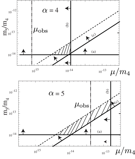
FIG. 5.: Constraints in the $\mu$-$m_{5}$ parameter space. Three solid lines are from (a) nucleosynthesis, (b) matter dominance at the decoupling time, and (c) the energy scale smaller than the 5-D Planck mass. The observation ($\Omega_{\phi}\sim 0.7$) fixes the value of $\mu$ ($\mu_{\rm obs}$), which is given by the vertical dot-dashed lines. If we assume that the potential energy of a scalar field is initially not very small compared with its kinetic energy, a successful quintessence is possible for a narrow range of parameters, which is shown by the shaded region.

Then if $\mu$ is fixed to find a scalar field dominance right now, the 5-dimensional Planck mass $m_{5}$ is limited. For example, for $\alpha=5$, if $\mu<10^{-14}m_{4}$, the constraint for $m_{5}$ is just coming from nucleosynthesis, while if $\mu>10^{-14}m_{4}$, $m_{5}>\mu$, which is stronger than that of nucleosynthesis.

Here we invoke a further constraint which could be derived from natural initial conditions. What would be the natural initial conditions for a scalar field? One plausible condition is an equipartition of each energy density. In this case, the radiation energy is larger than that of the scalar field because the degree of freedom of all particles $g$ is larger than that of the scalar field. How about the ratio of the kinetic energy to total one of the scalar field ? In the conventional quintessence scenario, the potential energy should be initially much smaller than the kinetic one. In the present model, it is not the case. This is because the attractor solution in the $\rho^{2}$-dominant stage reduces the density parameter of the scalar field. Therefore, we may impose natural initial conditions for a scalar field. To be more concrete, we focus on the potential by fermion condensation. After our 3-dimensional brane world is created, a fermion pair is condensed by a symmetry breaking mechanism and it behaves as a scalar filed with a potential $V(\phi)$. In this case, we expect that the potential term should play an important role from the initial stage.

We consider the cases for $\alpha=3,4,$ and 5. The initial conditions for a scalar field are classified into the following three cases. First, if the kinetic and potential energy of a scalar field are the same order of magnitude, the attractor solution is reached soon, and then we expect $\Omega_{\phi}^{(s)}\sim 0(g_{s}^{~{}-1})$, where $g_{s}$ is a degree of freedom of particles at $a_{s}$. Secondly, if the potential energy is dominant, it will not change so much before reaching the attractor solution, and then we expect that $\Omega_{\phi}^{(s)}\mbox{\raisebox{-4.30554pt}{$\stackrel{{\scriptstyle\textstyle>}}{{\textstyle\sim}}$}}0(g_{s}^{~{}-1})$. Thirdly, if the kinetic energy is larger than the potential one, it will decay soon, finding an attractor solution, then $\Omega_{\phi}^{(s)}\mbox{\raisebox{-4.30554pt}{$\stackrel{{\scriptstyle\textstyle<}}{{\textstyle\sim}}$}}0(g_{s}^{~{}-1})$, unless the kinetic energy dominates a lot, which we do not assume here. Therefore, a natural initial condition predicts $\Omega_{\phi}^{(s)}\sim 0(g_{s}^{~{}-1})$

From Eqs. (36) and (51), we find

$$\Omega_{\phi}^{(s)}=G(\alpha)\left({\mu\over m_{5}}\right)^{2(\alpha+4)\over(\alpha+2)}(m_{5}t_{s})^{-\frac{2\alpha}{\alpha+2}},$$ (59)

where $G(\alpha)=2^{{\alpha+4\over\alpha+2}}\alpha^{-{\alpha\over\alpha+2}}(\alpha+2)^{-{\alpha-2\over\alpha+2}}(6-\alpha)^{-{2\over\alpha+2}}/3$.

Since $\rho_{\rm r}(t_{s})\mbox{\raisebox{-4.30554pt}{$\stackrel{{\scriptstyle\textstyle<}}{{\textstyle\sim}}$}}m_{5}^{4}$, we have a constraint that $m_{5}t_{s}\mbox{\raisebox{-4.30554pt}{$\stackrel{{\scriptstyle\textstyle>}}{{\textstyle\sim}}$}}1.5$ from Eq. (51). This constraint with $\Omega_{\phi}^{(s)}\sim 0(g_{s}^{~{}-1})$ and $g_{s}\sim 10^{3}$ gives the lower bound for $\mu/m_{5}$ as

$$\mu \stackrel{{\scriptstyle\textstyle>}}{{\textstyle\sim}} 0.131m_{5}~{}~{}~{}{\rm for}~{}~{}\alpha=3,$$ (60)

$$\mu \stackrel{{\scriptstyle\textstyle>}}{{\textstyle\sim}} 0.140m_{5}~{}~{}~{}{\rm for}~{}~{}\alpha=4,$$ (61)

$$\mu \stackrel{{\scriptstyle\textstyle>}}{{\textstyle\sim}} 0.146m_{5}~{}~{}~{}{\rm for}~{}~{}\alpha=5.$$ (62)

With the previous constraint $\mu<m_{5}$, we find a narrow strip in the $\mu$-$m_{5}$ parameter space, which is shown by a shaded region in Fig.(5) The allowed region gets smaller for smaller values of $\alpha$. In particular, we find that no region is allowed for $\alpha\leq 3$. Therefore, the present model prefers a rather large value of $\alpha$.

The values of $\mu_{\rm obs}$, which explains the observed value of the dark energy now, are

$$\mu_{\rm obs} \sim 6.25\times 10^{-18}m_{4}~{}~{}~{}{\rm for}~{}~{}\alpha=3,$$ (63)

$$\mu_{\rm obs} \sim 8.75\times 10^{-16}m_{4}~{}~{}~{}{\rm for}~{}~{}\alpha=4,$$ (64)

$$\mu_{\rm obs} \sim 4.06\times 10^{-14}m_{4}~{}~{}~{}{\rm for}~{}~{}\alpha=5,$$ (65)

With these values, we find that there are no natural ranges for $\alpha\leq 4$. For $\alpha\mbox{\raisebox{-4.30554pt}{$\stackrel{{\scriptstyle\textstyle>}}{{\textstyle\sim}}$}}5$, the 5-dimensional Planck scale is strictly constrained from the observation because the allowed region is very narrow. For example, for $\alpha=5$, we find

$$4.06\times 10^{-14}m_{4}\mbox{\raisebox{-4.30554pt}{$\stackrel{{\scriptstyle\textstyle<}}{{\textstyle\sim}}$}}m_{5}\mbox{\raisebox{-4.30554pt}{$\stackrel{{\scriptstyle\textstyle<}}{{\textstyle\sim}}$}}2.78\times 10^{-13}m_{4}.$$ (66)

IV EXPONENTIAL POTENTIAL

Next we investigate an exponential potential model, i.e.

$$V(\phi)=\mu^{4}\exp\left[-\lambda\frac{\phi}{m_{4}}\right],$$ (67)

which is another typical potential for a quintessence [7],[9]. This type of potential is often found in unified theories of fundamental interactions of particles such as supergravity theory[25].

Within the conventional universe, this potential shows an interesting property, although in itself it may not provide a successful quintessence scenario. We first recall a few results[7],[9].

Suppose that a spatially flat FRW universe evolves with a scalar field $\phi$ and a background fluid of an equation of state $p_{B}=w_{B}\rho_{B}$. There exist just two possible attractor solutions, which show quite different late time properties, depending on the values of $\lambda$ and $w_{B}$ as follows:

1. For $\lambda^{2}>3(w_{B}+1)$, the scalar field mimics a barotropic fluid with $w_{\phi}\equiv p_{\phi}/\rho_{\phi}=w_{B}$, and the relation $\Omega_{\phi}\simeq\rho_{\phi}/\rho_{B}=3(w_{B}+1)/\lambda^{2}$ holds, where $\Omega_{\phi}$ is the density parameter of the scalar field.

2. If $\lambda^{2}<3(w_{B}+1)$, the late time attractor is a scalar field dominant solution ($\Omega_{\phi}=1$) with $w_{\phi}=-1+\lambda^{2}/3$.

Case 1 is the so-called scaling solution. If it is obtained in a radiation dominated era, a successful nucleosynthesis is possible for $\lambda^{2}>20$. However, the present observations of a scalar field dominance ($\Omega_{\phi}\simeq 0.7$) cannot be explained by this type of solution. Case 2 is preferred in the context of a quintessence scenario, but a scalar field behaves just as a cosmological constant in its evolution. Then, in order to explain $\Omega_{\phi}^{~{}(0)}\simeq 0.7$, an extreme fine-tuning in a choice of the initial value of a scalar field or in a mass scale $\mu$ is required just as the case of a cosmological constant. Therefore, some modification for this type of potential has been done by several authors for a successful quintessence[10], [11].

In the present paper, we study the effects of the quadratic term and see whether a natural initial condition is found. Hence, we will not analyze each modified potential quintessence model, but rather study the universal properties which are found in an exponential type potential. In particular, we are interested in case 2 above and see whether a fine-tuning is loosened by the present scenario.

The organization of this section is as follows: first, as in the previous section, we focus on the $\rho^{2}$-dominant stage, and we present an attractor solution which is expected to be found as its asymptotic behavior. This is confirmed by numerical analysis. Then, we discuss the possibility to improve a quintessence scenario by the effects of the quadratic term.

A Analytic solutions in the $\rho^{2}$-dominant stage

Since $m_{5}$ rather than $m_{4}$ is a fundamental parameter in the present model, it may be natural to introduce a new parameter $\tilde{\lambda}\equiv(m_{5}/m_{4})\lambda$, and to write the potential in the form of

$$V(\phi)=\mu^{4}\exp\left[-\tilde{\lambda}\frac{\phi}{m_{5}}\right].$$ (68)

In the brane world scenario, the value of $\tilde{\lambda}$ is expected to be of order unity, unless the potential is coming from other physical origin.

We discuss two initial conditions, a radiation dominant initial condition and a scalar-field dominant one, in that order.

$\left(1\right)$ radiation dominant initial condition

In the case of a radiation dominant era, the scale factor expands as $a\propto t^{1/4}$ and the equation for the scalar field (4) is now

$$\ddot{\phi}+\frac{3}{4t}\dot{\phi}-\left(\frac{\tilde{\lambda}\mu^{4}}{m_{5}}\right)\exp\left[-\tilde{\lambda}\frac{\phi}{m_{5}}\right]=0.$$ (69)

Since the exponential potential drops much faster than the inverse-power potential, unless $\phi\ll m_{5}/\tilde{\lambda}$, we expect that the kinetic energy dominant solution is asymptotically found as the case of the inverse-power potential with $\alpha>6$. Hence, assuming a kinetic energy dominant condition, we analyze the equations. Ignoring the potential term in Eq. (69), we find

$$\ddot{\phi}+\frac{3}{4t}\dot{\phi}=0,$$ (70)

which leads to the evolution of a scalar field as

$$\phi\propto t^{1/4}.$$ (71)

From this solution, $\rho_{\phi}^{~{}(K)}\propto t^{-3/2}$ and $\rho_{\phi}^{~{}(P)}\propto\exp(-t^{1/4})$ , where $\rho_{\phi}^{~{}(K)}$ and $\rho_{\phi}^{~{}(P)}$ denote a kinetic term of a scalar field and a potential one, respectively. This behavior confirms that the above kinetic-term dominant solution gives an asymptotic behavior of the scalar field.

However, for the case of $\phi\ll m_{5}/\tilde{\lambda}$, in particular for an extremely small value of $\tilde{\lambda}$, this potential behaves almost the same as a cosmological constant, and then the energy density of the scalar field will soon dominate radiation, although we cannot give its critical value quantitatively. However, as we will see later, it will again start to evolve into a radiation dominant solution as long as the $\rho^{2}$-term dominates. If the conventional universe is recovered before reaching the radiation dominant stage, then the radation dominance will never be obtained because the scalar field dominant solution is the attractor.

$\left(2\right)\phi$-dominant initial condition

If the scalar field dominates initially, the Friedmann equation (2) is

$$H=\frac{1}{6m_{5}^{\;3}}\left(\frac{1}{2}\dot{\phi}^{2}+\mu^{4}\exp\left[-\tilde{\lambda}\frac{\phi}{m_{5}}\right]\right),$$ (72)

while the equation for the scalar field (4) is

$$\ddot{\phi}+3H\dot{\phi}-\left(\frac{\tilde{\lambda}\mu^{4}}{m_{5}}\right)\exp\left[-\tilde{\lambda}\frac{\phi}{m_{5}}\right]=0.$$ (73)

We again expect that the kinetic term dominant solution gives an asymptotic behavior. Assuming the kinetic term dominant condition, from Eqs. (72) and (73), we find

$$\ddot{\phi}+\frac{1}{4m_{5}^{\;3}}\dot{\phi}^{3}=0,$$ (74)

which is the same as Eqs. (28) and (29), because the potential term does play no role. We find the same solution for a scalar field as before (Eq.(30)), and then the same result, i.e. this gives an asymptotic solution. Since radiation energy decreases slower than that of a massless scalar field, the universe will eventually evolve into a radiation dominant era, just as discussed in the previous section.

However, as discussed before, if $\tilde{\lambda}$ is extremely small, the potential does not decay so fast and then after recovering the conventional universe, a scalar field will lead to inflation.

B Numerical analysis

In order to show that the above kinetic term dominant solution in a radiation dominant era is a unique attractor for any initial condition, we present numerical results. In Fig.6, we depict the evolution of each energy density in the quadratic term dominant stage. In the top figure, we show the results for the initial condition of radiation dominance. We find that even for the initial conditions such that the potential term of a scalar field dominates the kinetic one, we eventually find a kinetic dominant solution. In the bottom, we also show the case of a scalar-field dominant initial condition. The universe eventually evolves into a radiation dominant era. Therefore, as long as $\tilde{\lambda}$ is of order unity, the solution obtained above is found asymptotically both from the radiation dominant initial condition and from the scalar-field dominant initial condition. We may conclude that radation dominance is a natural condition for the $\rho^{2}$-dominant stage.

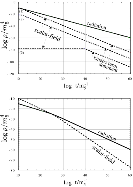
FIG. 6.: (Top) Time evolution of each energy density for $\tilde{\lambda}=1.0$ in the radiation dominant era. The kinetic term dominant solution is realized for any initial conditions including the case of potential dominance. As for the initial conditions, we set $\rho_{\rm r}=1.0\times 10^{-10}m_{5}^{\;4},\rho_{\phi}^{~{}(K)}=0.0,\rho_{\phi}^{~{}(P)}=1.39\times 10^{-11}m_{5}^{\;4},$ for (1), $\rho_{\phi}^{~{}(K)}=0.0,\rho_{\phi}^{~{}(P)}=4.22\times 10^{-22}m_{5}^{\;4},$ for (2), $\rho_{\phi}^{~{}(K)}=0.0,\rho_{\phi}^{~{}(P)}=6.71\times 10^{-79}m_{4}^{\;4},$ for (3). (Bottom) Time evolution of each energy density for $\tilde{\lambda}=1.0$, starting from the scalar-field dominant initial condition. As for the initial condition, we set $\rho_{\rm r}=1.0\times 10^{-15}m_{5}^{\;4},\rho_{\phi}^{~{}(K)}=0.0,\rho_{\phi}^{~{}(P)}=1.39\times 10^{-11}m_{5}^{\;4}.$ The kinetic term dominates the energy density of a scalar field soon, and the radiation dominance is eventually reached.

C A quintessence scenario

Although a pure exponential potential may not give a natural quintessence model, we shall study whether or not a similar mechanism for the value of $\Omega_{\phi}$ in the $\rho^{2}$-dominant stage works. If it works, it may provide a natural initial condition for a quintessence model based on an exponential potential. We discuss two cases; (a) $\tilde{\lambda}\sim O(1)$ and (b) $\lambda\sim O(1)$ in order.

Case (a) : Suppose $\tilde{\lambda}\sim O(1)$ because the potential causes the 5-dimensional origin. In this case, as we discussed above, the radiation dominant universe is an attractor and the kinetic term dominates the potential for a scalar field. When the universe evolves into the conventional expansion stage, the scalar field approaches an attractor of a scaling solution soon, because $\lambda=(m_{4}/m_{5})\tilde{\lambda}\gg 1$. In fact, we find $\lambda>10^{14}$ from the constraint on $m_{5}$ by nucleosynthesis. The ratio of the scalar field energy to radation energy, which is fixed by $\lambda$ as $\Omega_{\phi}\simeq\rho_{\phi}/\rho_{B}=3(w_{B}+1)/\lambda^{2}$, turns out to be very small in the present model. Therefore, this does not provide any quintessence model. In order to remedy it, we may need an additional potential for quintessence models with exponential type potentials in the conventional universe[11]. For example, suppose that the potential is $V(\phi)=\mu^{4}\exp[-\tilde{\lambda}\phi/m_{5}]+\mu_{2}^{4}\exp[\lambda_{2}\phi/m_{4}]$. If $\mu_{2}\sim 10^{-30}m_{4}$, we find that min($V$) $\sim\mu_{2}^{4}\sim\rho_{\rm cr}$, which gives the present small cosmological constant. However, an introduction of such an additional potential may break naturalness in the present model.

Case (b) : If we have $\lambda\sim O(1)$,i.e. $\tilde{\lambda}\sim\frac{m_{5}}{m_{4}}\ll 1$, the potential may behave as a cosmological constant in $\rho^{2}$-dominant stage. We show for the case with initial conditions that $\rho_{r}>\rho_{\phi}$ (Fig.7). The energy density of the scalar field remains constant and eventually dominates the radiation, leading to the inflationary stage, unless the conventional universe is recovered. Hence this does not change the conventional quintessence model with exponential potential. If the kinetic term dominates in the energy density of a scalar field, however, the energy density will decrease in time.

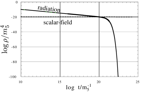
FIG. 7.: The time evolution of the energy densities for extremely small $\tilde{\lambda}$, in which case the scalar field behaves as the cosmological constant. Even though starting from a radiation dominant initial condition, the scalar field dominates the radiation, and inflation happens. In this case, we take $\tilde{\lambda}=1.0\times 10^{-14}$. As for the initial condition, we set $\rho_{\rm r}=1.0\times 10^{-10}m_{5}^{\;4},\rho_{\phi}^{~{}(K)}=0.0,\rho_{\phi}^{~{}(P)}=1.50\times 10^{-20}m_{5}^{\;4}.$

We then study this case in what follows. We have to know the value of $V(\phi(a_{c}))$, which is approximately the present value of a cosmological constant, because the potential term remains almost constant as a cosmological constant after the universe enters the conventional expansion stage. The evolution for a scalar field in the $\rho^{2}$-dominant stage is given by Eq.(71), i.e. $\phi\propto a\propto 1/T$.

$$V(\phi(a_{c})) \sim V(\phi(a_{s}))\exp\left[-\lambda\phi_{c}/m_{4}\right]$$ (75)

$$\sim V(\phi(a_{s}))\exp\left[-\lambda{\phi_{s}T_{s}\over m_{5}^{2}}\left({m_{5}\over m_{4}}\right)^{1/2}\right].$$ (76)

In order to find $V(\phi(a_{c}))\sim\rho_{\rm cr}$, the exponent in the r.h.s. in Eq.(76) should be very large. However, since $m_{5}\ll m_{4}$, the initial value of $\phi_{s}$ should be large as

$$\phi_{s}\mbox{\raisebox{-4.30554pt}{$\stackrel{{\scriptstyle\textstyle>}}{{\textstyle\sim}}$}}10^{2}\left({m_{4}\over m_{5}}\right)^{1/2}m_{5}.$$ (77)

This initial condition may not be natural.

We may conclude that for exponential type potential, a brane world does not improve the quintessence scenario.

V KINETICALLY DRIVEN QUINTESSENCE

There is another type of quintessence model in the conventional universe, in which the quintessential dynamics is driven solely by a (non-canonical) kinetic term rather than by a potential term[26],[27] . It is called ”k-essence”. Here we shall study it in the context of a brane world.

The model Lagrangian of a scalar field is given by

$$S=\int d^{4}x\sqrt{-g}\left[-K(\phi)X+L(\phi)X^{2}\right],$$ (78)

where $X={1\over 2}\left(\nabla\phi\right)^{2}$. If we introduce a new scalar field by

$$\Phi=\int\sqrt{L\over|K|}d\phi,$$ (79)

the action (78) is rewritten as

$$S=\int d^{4}x\sqrt{-g}f(\Phi)\left[-X+X^{2}\right].$$ (80)

Among them, the model defined by

$$f(\Phi)=\mu^{4-\alpha}\Phi^{-\alpha},$$ (81)

provides a ”tracking” solution[26]. $\mu$ is a typical mass scale of the system and will fix when the scalar field dominates. We then expect a similar or more interesting feature in the $\rho^{2}$-dominant stage. It may provide more natural initial conditions as the inverse power-law potential discussed in §3. Note that a scalar field $\Phi$ has not mass dimension but inverse-mass dimension.

Contrary to our expectation, however, we do not find a solution for which the density parameter of a scalar field decreases. Instead, as an attractor, we have a “tracking solution” in which the density parameter increases slower than that in the conventional universe. Furthermore, we find a ”scaling” solution as a transient attractor in the radiation dominant era.

A Analytic solutions

$\left(1\right)$ Model

First, we shortly explain our quintessence model with Eqs. (80) and (81). Assuming the FRW universe model, the “pressure”, $p_{\Phi}$, and the “energy density”, $\rho_{\Phi}$, of a quintessence scalar field $\Phi$ is given by

$$p_{\Phi}=\mu^{4-\alpha}\Phi^{-\alpha}\left(-X+X^{2}\right),$$ (82)

$$\rho_{\Phi}=\mu^{4-\alpha}\Phi^{-\alpha}\left(-X+3X^{2}\right),$$ (83)

where $X=(1/2)\dot{\Phi}^{2}$. Note that in order to guarantee the positive energy density of the scalar field , $\rho_{\Phi}$, it is necessary that $\dot{\Phi}^{2}>(2/3)$.

The field equation corresponding to (4) is

$$\ddot{\Phi}(1-3\dot{\Phi}^{2})+3H(1-\dot{\Phi}^{2})\dot{\Phi}-\frac{\alpha}{4\Phi}(2-3\dot{\Phi}^{2})\dot{\Phi}^{2}=0,$$ (84)

Since this equation has a reflection symmetry ($\Phi\leftrightarrow-\Phi$), we discuss only the case of $\Phi>0$.

$\left(2\right)$ Analytic solutions in the conventional cosmology

First we show two analytic solutions in the conventional cosmology. We assume the radiation dominant era, even though a similar solution is found in the matter dominant era.

Then the scale factor expands as $a\propto t^{1/2}$ and the equation for the scalar field is Eq. (84) with $H=1/2t$.

We have two analytic solutions: (a) a tracking solution, which is exact and is an attractor, and (b) a scaling solution, which is approximate and a transient attractor.

(a) a tracking solution: For Eq.(84) with $H=1/2t$ , we have an exact solution for $\alpha<2$ or for $\alpha>3$ as

$$\Phi=\sqrt{\frac{2(3-\alpha)}{3(2-\alpha)}}t,$$ (85)

which yields its energy density as

$$\rho_{\Phi}=\frac{\mu^{4-\alpha}}{2(2-\alpha)}\left[\frac{2(3-\alpha)}{3(2-\alpha)}\right]^{(2-\alpha)/2}t^{-\alpha}\propto a^{-2\alpha}.$$ (86)

For $\alpha<2$, the energy density of the scalar field decreases slower than that of radiation, i.e. the density parameter $\Omega_{\Phi}$ increases as $a^{2(2-\alpha)}$. This solution is the tracking solution.

For $\alpha>3$, the energy density becomes negative, although the density parameter $\Omega_{\Phi}=|\rho_{\Phi}/\rho_{\rm r}|$ decreases. This solution may not be interesting for a quintessence scenario because the scalar field energy never dominates.

(b) a scaling solution: Another interesting solution is found in the limit of $\dot{\Phi}^{2}\gg 1$. In this case, the equation for a scalar field (84) with $H=1/2t$ is

$$\ddot{\Phi}+\frac{1}{2t}\dot{\Phi}-\frac{\alpha}{4\Phi}\dot{\Phi}^{2}=0.$$ (87)

It is easy to find a solution for Eq. (87),which is

$$\Phi\propto t^{2/(4-\alpha)}~{}~{}~{}{\rm and}~{}~{}~{}\dot{\Phi}\propto t^{-(2-\alpha)/(4-\alpha)}.$$ (88)

The coefficient is an integration constant and depends on the initial condition. The energy density is now

$$\rho_{\Phi}\propto t^{-2}\propto a^{-4},$$ (89)

This is nothing but a scaling solution in a radiation dominant era.

We easily show that this solution is an attractor in the present system with the approximation of $\dot{\Phi}^{2}\gg 1$. However, this solution (88) shows that the approximation will be eventually broken because $\dot{\Phi}$ decreases. Hence, after this approximation becomes invalid, the universe evolves into the tracking solution. Note that for $\alpha<3$, $\dot{\Phi}$ increases and the approximation is always valid, although the energy density is negative.

$\left(3\right)$ Analytic solutions in the $\rho^{2}$-dominant stage

In the $\rho^{2}$-dominant stage, assuming the radiation dominant era, i.e. the evolution of the scale factor is $a\propto t^{1/4}$, the equation for a scalar field is given by Eq. (84) with $H=1/4t$.

The same as in the conventional universe, we have two analytic solutions: (a) a tracking solution, which is exact and an attractor, and (b) a scaling solution, which is approximate and a transient attractor.

(a) a tracking solution: There is an exact solution for $\alpha<1$ or for $\alpha>3/2$, which is

$$\Phi=\sqrt{\frac{3-2\alpha}{3(1-\alpha)}}t,$$ (90)

which yields the energy density of a scalar field as

$$\rho_{\Phi}={\mu^{4-\alpha}\over 4(1-\alpha)}\left[\frac{3-2\alpha}{3(1-\alpha)}\right]^{(2-\alpha)/2}t^{-\alpha}\propto a^{-4\alpha}.$$ (91)

The density parameter $\Omega_{\Phi}$ increases as $a^{4(1-\alpha)}$ for $\alpha<1$. This solution is again a tracking solution, although the rate of increase is smaller than that in the conventional universe. There is no solution in which $\Omega_{\Phi}$ decreases. This is a big difference between the present model and the model with inverse-power potential. For the case of $\alpha>3/2$, $\rho_{\Phi}$ becomes negative. Since the positivity of the energy density of a scalar field is not guaranteed, it might be allowed if the Friedmann equation is not contradicted as in the case of a radiation dominant era. Although it might be interesting because the density parameter $\Omega_{\Phi}$ decreases, it turns out that such a solution cannot evolve into a tracking solution in the conventional universe [26]. Hence, we do not discuss this solution in what follows.

(b) a scaling solution: We have another solution in the limiting case of $\dot{\Phi}^{2}\gg 1$. The equation for the scalar field

$$\ddot{\Phi}+\frac{1}{4t}\dot{\Phi}-\frac{\alpha}{4\Phi}\dot{\Phi}^{2}=0.$$ (92)

has an analytic solution

$$\Phi\propto t^{3/(4-\alpha)}~{}~{}~{}{\rm and}~{}~{}~{}\dot{\Phi}\propto t^{-(1-\alpha)/(4-\alpha)},$$ (93)

and

$$\rho_{\Phi}\propto t^{-1}\propto a^{-4},$$ (94)

which is a scaling solution. Since $\dot{\Phi}$ decreases as Eq.(93), the approximation of $\dot{\Phi}^{2}\gg 1$ will be eventually broken. This scaling solution is a transient attractor. Then, a tracking solution will be finally reached for $\alpha<1$. Since there is no attractor solution for $\alpha\geq 1$, the evolution of a scalar field may depend on the initial conditions. Once the universe evolves into the conventional expansion stage, however, the scalar field begins to approach an attractor solution.

Next, we investigate the case of the scalar-field dominant era. The Friedmann equation (2) is given by

$$H=\frac{1}{6m_{5}^{\;3}}\mu^{4-\alpha}\Phi^{-\alpha}\left(-X+3X^{2}\right).$$ (95)

In the limit of $\dot{\Phi}^{2}\gg 1$, we find a power law solution as

$$a \propto t^{1\over 4}$$ (96)

$$\Phi = {\Phi_{0}\over\mu}(\mu t)^{3\over(4-\alpha)},$$ (97)

where a dimensionless constant $\Phi_{0}$ is given by

$$\Phi_{0}=2^{1\over 4-\alpha}\left(\frac{\mu}{m_{5}}\right)^{-{3\over 4-\alpha}}\left(\frac{4-\alpha}{3}\right)^{4\over 4-\alpha}.$$ (98)

Then the energy density of the scalar field is given by

$$\rho_{\Phi}=\frac{3}{2}m_{5}^{3}t^{-1}\propto a^{-4},$$ (99)

which drops as the radiation energy. Hence, once this solution is reached, contrary to the case of inverse-power law potential, the radiation never dominates the scalar field. Therefore, a scalar field dominant initial condition does not provide a successful quintessence scenario.

B Numerical analysis

In order to confirm the above analysis, we shall show our numerical results. The initial condition is chosen such that the inequality $\dot{\Phi}^{2}>2/3$ is satisfied, which guarantees positivity of the energy density of a scalar field. First, we show the case with radiation dominant initial conditions in Fig.8. We find that a tracking solution (90) or a scaling solutions (93) is really an attractor or a transient one.

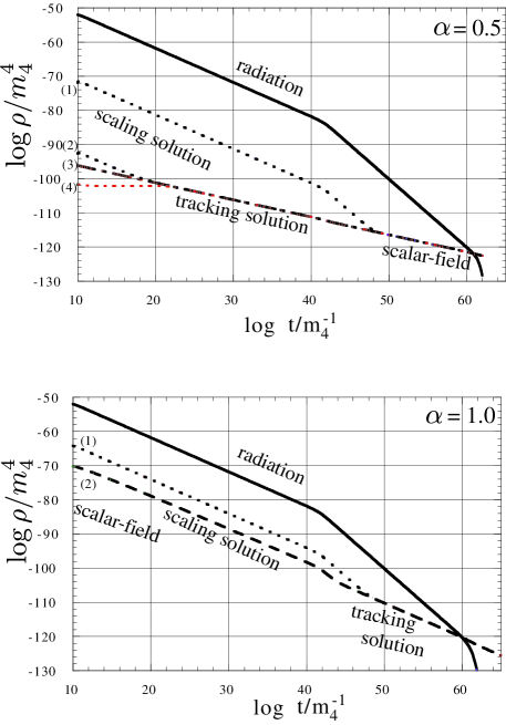
FIG. 8.: (Top) Time evolution of each energy density for $\alpha=0.5$. We set $\mu=1.0\times 10^{-26}m_{4},m_{5}=1.0\times 10^{-14}m_{4}$. As for initial conditions, we set $\rho_{\rm r}=1.0\times 10^{-52}m_{4}^{\;4}$, and $\rho_{\Phi}=1.24\times 10^{-72}m_{4}^{\;4}$ ($\Phi=1.15\times 10^{10}m_{4}^{\;-1},X=6.67\times 10^{11}$), $1.96\times 10^{-93}m_{4}^{\;4}$ ($\Phi=1.15\times 10^{3}m_{4}^{\;-1},X=6.67\times 10^{-1}$), $6.21\times 10^{-97}m_{4}^{\;4}$ ($\Phi=1.15\times 10^{10}m_{4}^{\;-1},X=6.67\times 10^{-1}$) , and $1.95\times 10^{-102}m_{4}^{\;4}$ ($\Phi=1.15\times 10^{21}m_{4}^{\;-1},X=6.67\times 10^{-1}$) for (1), (2), (3) and (4), respectively. It is easy to see that the tracking solution is an attractor, while the scaling solution is a transient attractor. (Bottom) The same figure as the top for $\alpha=1$. We set $\mu=1.0\times 10^{-20}m_{4},m_{5}=1.0\times 10^{-14}m_{4}$. As for initial conditions, we set $\rho_{\rm r}=1.0\times 10^{-52}m_{4}^{\;4}$, and $\rho_{\Phi}=5.77\times 10^{-65}m_{4}^{\;4}$ ($\Phi=1.15\times 10^{4}m_{4}^{\;-1},X=6.67\times 10^{-1}$), $5.77\times 10^{-71}m_{4}^{\;4}$ ($\Phi=1.15\times 10^{10}m_{4}^{\;-1},X=6.67\times 10^{-1}$) for (1), (2) , respectively. There is no attractor solution in the $\rho^{2}$-dominant stage. After the conventional cosmology is recovered, the scaling solution evolves into a tracking solution.

Next, we show numerical results for the scalar field dominant initial conditions in Fig.9. The energy density of the radiation never dominates that of the scalar field, and there exists no radiation dominant era, which is excluded from the constraint of nucleosynthesis.

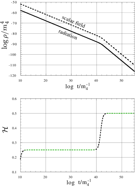
FIG. 9.: (Top) Time evolution of the energy densities with the scalar field dominant initial conditions for $\alpha=1$. As for initial conditions, we set $\rho_{\rm r}=1.0\times 10^{-58}m_{4}^{\;4}$ and $\rho_{\Phi}=1.12\times 10^{-52}m_{4}^{\;4},$ ($\Phi=1.66\times 10^{19}m_{4}^{\;-1},X=2.45\times 10^{13}$). Note that both energy densities drop as $\propto t^{-1}$ in the $\rho^{2}$-dominant era and $\propto t^{-2}$ in the conventional universe. (Bottom) The change of the power of scale factor, ${\cal H}=Ht$. Even in a scalar field dominant universe, the cosmic expansion is the same as that of the radiation, i.e. $a\propto t^{1/4}$ the $\rho^{2}$-dominant era and $t^{1/2}$ in the conventional universe. We set $\mu=1.0\times 10^{-20}m_{4},m_{5}=1.0\times 10^{-14}m_{4}.$

C Constraint to the model

Now, we discuss the value of the parameter $\mu$. For a successful quintessence, i.e. in order for a scalar field to dominate the energy density right now, we have to tune the value of $\mu$. Naive estimation gives

$$\rho_{\Phi 0}=\mu^{4-\alpha}\Phi^{-\alpha}_{0}\left(-X_{0}+3X_{0}^{2}\right)\simeq\rho_{\rm(cr)0},$$ (100)

where $\Phi_{0}$ and $X_{0}$ are the present values of $\Phi$ and $X$, and $\rho_{\rm(cr)0}$ is the present value of the critical density.

The present value of the scalar field is estimated by a tracking solution in the matter dominant era, which is

$$\Phi=\sqrt{\frac{2(4-\alpha)}{8-3\alpha}}t.$$ (101)

Since $H_{0}\sim 2/3t_{0}$, we find

$${\Phi_{0}}^{-1} = \frac{3}{2}H_{0}\sqrt{\frac{8-3\alpha}{8-2\alpha}}\simeq H_{0},$$ (102)

$$X_{0} = \frac{(4-\alpha)}{8-3\alpha}\sim O(1)$$ (103)

for $0<\alpha<8/3$. These equations with Eq. (100) fix $\mu$ and the present value of the scalar field as

$$\mu\sim 10^{(43\alpha-48)/(4-\alpha)}[{\rm GeV}],$$ (104)

$$\Phi_{0}\sim 10^{43}[{\rm GeV}^{-1}].$$ (105)

If the mass scale $\mu$ is the same order of magnitude as the five-dimensional Planck mass $m_{5}$, we have a constraint on the value of $\alpha$ from nucleosynthesis, i.e. $m_{5}\mbox{\raisebox{-4.30554pt}{$\stackrel{{\scriptstyle\textstyle>}}{{\textstyle\sim}}$}}10^{4}$ GeV, that is $\alpha\geq 1.4$.

VI Summary and Discussion

In this paper, we have studied quitessence models in a brane world scenario. We have adopted the second Randall-Sundrum brane scenario for a concrete model, although a similar result would be obtained in other brane world models. As a consequence of a brane embedded in the extra-dimension, the quadratic term of energy density appears, changing the expansion law in the early stage of the universe. This affects the dynamics of the scalar field in the quadratic-term dominant stage. We have then investigated three candidates for a successful quintessence.

As a first candidate, we have discussed an inverse-power-law potential model, $V=\mu^{4+\alpha}\phi^{-\alpha}$ with $2<\alpha<6$. We have shown the solution in which the density parameter of a scalar field decreases as $a^{-4(\alpha-2)/(\alpha+2)}$ in the $\rho^{2}$-dominant stage. This feature provides us wider initial conditions for a successful quintessence. In fact, even if the universe is initially in a scalar-field dominant, it eventually evolves into the radiation dominant era in the $\rho^{2}$-dominant stage, which guarantees a successful nucleosynthesis in the conventional universe stage.

Although initial conditions could be arbitrary because the present solution is an attractor, we may have a natural initial condition for some specific origin of a potential such as a fermion condensation. If this is the case, equipartition of each energy density is more likely. Assuming such an equipartition, we have shown constraints in $\mu-m_{5}$ plane for a natural and successful quintessence scenario. The allowed region gets wider as $\alpha$ is larger, because for larger $\alpha$, the density parameter becomes smaller when the conventional cosmology is recovered. We conclude that in order to explain naturally the observational value of the dark energy by the present scenario, $\alpha\geq 4$ is required. This constraint also restricts the value of the 5-dimensional Planck mass, e.g. for $\alpha=5$, $4.06\times 10^{-14}m_{4}\mbox{\raisebox{-4.30554pt}{$\stackrel{{\scriptstyle\textstyle<}}{{\textstyle\sim}}$}}m_{5}\mbox{\raisebox{-4.30554pt}{$\stackrel{{\scriptstyle\textstyle<}}{{\textstyle\sim}}$}}2.78\times 10^{-13}m_{4}$.

We have also discussed an exponential potential model $V=\mu^{4}\exp(-\lambda\phi/m_{4})$, although by itself it may not provide a successful quintessence scenario. In the five-dimensional brane scenario, $\tilde{\lambda}=\lambda m_{5}/m_{4}$ is expected to be order unity. If that is the case, the kinetic term of the scalar field becomes eventually dominant for any initial conditions, and the density parameter of the scalar field decreases in the quadratic-term dominant stage. In this case, however, $\lambda$ becomes too large to explain the present scalar field dominance. We may need unnatural modification in the potential. On the other hand, if $\lambda\sim O(1)$ to find a successful quintessence scenario in the conventional universe stage, $\tilde{\lambda}$ becomes very large. This provides an extremely flat potential, which behaves just as a cosmological constant in the $\rho^{2}$-dominant stage, resulting in an inflationary expansion before reaching the conventional universe. After that, the radiation never dominates, which contradicts nucleosynthesis. Therefore, in both cases, we may not find a natural and successful quintessence scenario.

As a third model, we have investigated a kinetic-term quintessence (the so-called $k$-essence) model. We have adopted a model with an inverse-power-law potential in coefficients of kinetic terms. This provides a tracking solution just the same as the case with an inverse- power-law potential. We then expect to obtain a natural quitessence scenario. Contrary to our expectation, however, we do not find any solution in $\rho^{2}$-dominant stage by which the density parameter $\Omega_{\Phi}$ decreases. Instead, we find a tracking solution in which density parameter increases more slowly than that in the conventional universe. We also find a scaling solution which is a transient attractor. Then, if the universe starts with radiation dominance, the density parameter keeps constant in the early stage and then the universe moves to a tracking solution, finding a usual $k$-essence in the conventional universe. We do not find so much advantage in a brane world. Only the density parameter increases more slowly in the $\rho^{2}$-dominant stage, which provides a wider initial condition for a sucsessful quintessence. Finally , we have shown the value of the parameter $\mu$ appeared in this model can be taken as the same order as the five-dimensional Planck mass scale if $\alpha\geq 1.4$.

REFERENCES

- [1] P. de Bernardis et al. , Nature 404, 955 (2000); A. E. Lange et al., Phys. Rev. D 63, 042001 (2001); A. Balbi et al., Ap. J. 545, L1 (2000).
- [2] S. Perlmutter et al., Nature 391, 51 (1998); A. G. Riess et al., Astron. J. 116, 1009 (1998); P. M. Garnavich et al., Ap. J. 509, 74 (1998); S. Perlmutter et al. , Ap. J. 517, 565 (1999).
- [3] Weinberg, Rev. Mod. Phys. 61, 1 (1989); V. Sahni and A. Starobinsky, Int. J. Mod. Phys. D 9, 373 (2000) ; S. Weinberg, astro-ph/0005265.
- [4] A. D. Dolgov, in The Very Early Universe (eds. G. W. Gibbons et al. , Cambridge University Press), 449 (1982); L. H. Ford, Phys. Rev. D 35, 2339 (1987); S. M. Barr, Phys. Rev. D 36, 1691 (1987); Y. Fujii and T. Nishioka, Phys. Rev. D 42, 361(1990); K. Coble, S. Dodelson and J. A. Frieman, Phys. Rev. D 55, 1851 (1997).
- [5] J. M. Overduin and F. I. Cooperstock, Phys. Rev. D 58, 043506 (1998).
- [6] R. R. Caldwell, R. Dave and P. J. Steinhardt, Phys. Rev. Lett. 80, 1582 (1998); L. Wang, R. R. Caldwell, J. P. Ostriker and P. J. Steinhardt, Astrophys. J. 530,17 (2000).
- [7] B. Ratra and P. J. E. Peebles, Phys. Rev. D 37, 3406 (1988) ; A.R. Liddle and R. J. Scherrer Phys. Rev. D 59, 023509 (1998).
- [8] I. Zlatev, L. Wang and P. J. Steinhardt, Phys. Rev. Lett. 82, 896 (1999); P. J. Steinhardt, L. Wang and I. Zlatev, Phys. Rev. D 59, 123504 (1999).
- [9] P. G. Ferreira and M. Joyce, Phys. Rev. D 58, 023503 (1998); E. J. Copeland, A. R. Liddle and D. Wands, Phys. Rev. D 57, 4686 (1998); P. G. Ferreira and M. Joyce, Phys. Rev. Lett. 79, 4740 (1997); P. Viana and A. Liddle, Phys. Rev. D 57, 674 (1998).
- [10] Y. Fujii, Phys. Rev. 62, 064004 (2000); L. Amendola, Phys. Rev. D 62, 043511 (2000); A.Albrecht and C. Skordis, Phys. Rev. Lett. 84, 2076 (2000); S. Dodelson, M. Kaplinghat and E. Stewart, Phys. Rev. Lett. 85, 5276 (2000).
- [11] T. Barreiro, E. J. Copeland and N. J. Nunes, Phys. Rev. D 61, 127301 (2000); V. Sahni and L. Wang, Phys. Rev. D 62, 103517 (2000).
- [12] N. Arkani-Hamed, S. Dimopoulos and G. Dvali, Phys. Lett. B 429, 263 (1998); I. Antoniadis, N. Arkani-Hamed, S. Dimopoulos and G. Dvali, Phys. Lett. B 436, 257 (1998).
- [13] P. Hoava and E. Witten, Nucl. Phys. B 460, 506 (1996); ibid B 475, 94 (1996).
- [14] L. Randall and R. Sundrum, Phys. Rev. Lett. 83, 4690 (1999); L. Randall and R. Sundrum, Phys. Rev. Lett. 83, 3370 (1999).
- [15] V. A. Rubakov and M. E. Shaposhinikov, Phys. Lett. B 125, 139 (1983); K. Akama, in Gauge Theory and Gravitation ed by K. Kikkawa, N. Nakanishi, and H. Nariai (Springer-Verlag, 1983); K. Akama, hep-th/0001113.
- [16] T. Shiromizu, K. Maeda, and M. Sasaki, Phys. Rev. D 62, 024012 (2000).
- [17] R. Maartens, gr-qc/0101059.
- [18] P. Bintruy, C. Deffayet and D. Langlois, Nucl. Phys. B 565, 269 (2000); N. Kaloper, Phys. Rev. D 60, 123506 (1999) ; C. Csaki, M. Graesser, C. Kolda and J. Terning Phys. Lett. B 462, 34 (1999) ; T. Nihei, Phys. Lett. B 465, 81 (1999) ; P. Kanti, I. I. Kogan, K. A. Olive and M. Prospelov, Phys. Lett. B 468, 31 (1999); J. M. Cline, C. Grojean and G. Servant, Phys. Rev. Lett. 83, 4245 (1999); P. Bintruy, C. Deffayet, U. Ellwanger and D. Langlois, Phys. Lett. B 477, 285 (2000) ; S. Mukohyama, T. Shiromizu and K. Maeda, Phys. Rev. D 62, 024028 (2000).
- [19] R. Maatens, D. Wands, B. A. Bassett and I. P. C. Heard, Phys. Rev. D 62, 041301 (2001); L. Mendes and A. R. Liddle, Phys. Rev. D 62, 103511 (2000); J. Khoury, P. J. Steinhardt and D. Waldram, Phys. Rev. D 63, 103505 (2001); A. Mazumdar Nucl. Phys. B 597, 561 (2001); R. M. Hawkins and J. E. Lidsey, Phys. Rev. D 63, 041301 (2001); S. Tsujikawa, K. Maeda and S. Mizuno, Phys. Rev. D, 63 ,123511 (2001); S. C. Davis, W. B. Perkins, A.-C. Davis and I.R. Vernon, Phys. Rev. D 63, 083518 (2001).
- [20] E. J. Copeland, A. R. Liddle and J. E. Lidsey, astro-ph/0006421 ; G. Huey and J. E. Lidsey, astro-ph/0104006.
- [21] K. Maeda, astro-ph/0012313.
- [22] K. Maeda, and D. Wands, Phys. Rev. D 62, 124009 (2000).
- [23] P. Bintruy, Phys. Rev. D 60, 063502 (1999); P. Brax and J. Martin, Phys. Rev. D 61, 103502 (2000); T. R. Taylor, G. Veneziano and S. Yankielowicz, Nucl. Phys. B 218, 493 (1983); I. Affleck, M. Dine and N. Seiberg, Nucl. Phys. B 256, 557 (1985).
- [24] K. Maeda, S. Mizuno and K.Yamamoto, in preparation.
- [25] B. Whitt, Phys. Lett. B 145, 176 (1984); J. D. Barrow and S. Cotsakis, Phys. Lett. B 214, 515 (1988); D. Wands, Class. Quantum Grav. 11,269 (1994); M. B. Green, J. H. Schwarz, and E. Witten, Superstring Theory ( Cambridge University Press, Cambridge, England, 1987).
- [26] T. Chiba, T. Okabe and M. Yamaguchi, Phys. Rev. D 62, 023511.
- [27] C. Armendariz-Picon, V. Mukhanov and P. J. Steinhardt, Phys. Rev. Lett. 85, 4438 (2000).