$B\rightarrow X_{s}\gamma$ in Supersymmetry with Explicit CP Violation

Abstract

We discuss $B\to X_{s}\gamma$ decay in both constrained and unconstrained supersymmetric models with explicit CP violation within the minimal flavor violation scheme by including $\tan\beta$–enhanced large contributions beyond the leading order. In this analysis, we take into account the relevant cosmological and collider bounds, as well as electric dipole moment constraints. In the unconstrained model, there are portions of the parameter space yielding a large CP asymmetry at leading order (LO). In these regions, we find that the CP phases satisfy certain sum rules, e.g., the sum of the phases of the $\mu$ parameter and the stop trilinear coupling centralize around $\pi$ with a width determined by the experimental bounds. In addition, at large values of $\tan\beta$, the sign of the CP asymmetry tracks the sign of the gluino mass, and the CP asymmetry is significantly larger than the LO prediction. In the constrained minimal supersymmetric standard model based on minimal supergravity, we find that the decay rate is sensitive to the phase of the universal trilinear coupling. This sensitivity decreases at large values of the universal gauino mass. We also show that for a given set of the mass parameters, there exists a threshold value of the phase of the universal trilinear coupling which grows with $\tan\beta$ and beyond which the experimental bounds are satisfied. In both supersymmetric scenarios, the allowed ranges of the CP phases are wide enough to have phenomenological consequences.

I Introduction

One of the best motivated extensions of the standard model (SM) is softly broken supersymmetry (SUSY) which provides novel sources for flavor and CP violation [1] beyond the Cabibbo–Kobayashi–Maskawa (CKM) picture. While flavor violation may come from the intergenerational entries of the soft sfermion masses and tri-linear scalar couplings, their phase content as well as the phases of the $\mu$ parameter and gaugino masses provide sources for CP violation. Flavor-changing neutral current data puts stringent bounds on flavor mixings [2]; therefore, such entries must be suppressed as would be the case if the same unitary rotation which diagonalizes the quark mass matrices also diagonalizes the squark mass matrices in flavor space. In this minimal flavor violation (MFV) scheme, which is naturally realized in gravity mediated supersymmetry breaking and no scale models, flavor violation is minimal as it is generated only by the CKM matrix. In contrast, the CP violation is not minimal as it can spring from both the CKM matrix which leads to flavor–changing processes ($e.g.$ the CP asymmetry in $B\rightarrow X_{s}\gamma$ decay) and from the flavor–blind CP phases of the soft SUSY–breaking masses with flavor–conserving processes ($e.g.$ electric dipole moments (EDMs)) [1].

The effects of the SUSY CP–violation can be manifest in several observables such as: the mixing of the Higgs bosons [3], EDMs [4, 5, 6, 7, 8], lepton polarization asymmetries in semileptonic decays [9], the formation of P–wave charmonium and bottomonium resonances [10], and CP violation in $B$ meson decays [11, 12, 13] and mixings [14]. Among these observables, the most constraining are the EDMs [15, 16, 17] which bound the argument of the $\mu$ parameter to be $\mathrel{\raise 1.29167pt\hbox{$<$\kern-7.5pt\lower 4.30554pt\hbox{$\sim$}}}\pi/(5\tan\beta)$, leaving the other SUSY phases mostly unconstrained, in both constrained [6, 7, 8] and unconstrained [4, 5, 7, 8] supersymmetry. The constraint on the phase of the $\mu$ parameter is lifted if the sfermions of the first two generations weigh $\gg{\rm TeV}$ as in the effective SUSY scenario [18] though the EDMs are regenerated at the two–loop level, and can still compete with the experimental bounds [19] in certain portions of the parameter space.

The rare radiative inclusive $B$ meson decay, $B\rightarrow X_{s}\gamma$ provides a powerful test of the standard model (SM) and “new physics” such as supersymmetry. The drive to reduce theoretical uncertainties has led to the computation of next–to–leading order (NLO) terms in the SM [20] and two–doublet models [21], and a partial computation to the same order in supersymmetry (SUSY) [22, 23]. The measurements of the branching ratio at CLEO [24], ALEPH [25] and BELLE [26] give the combined result

$$\mbox{BR}\left(B\rightarrow X_{s}\gamma\right)=\left(3.11\pm 0.42\pm 0.21\right)\times 10^{-4}$$ (1)

whose agreement with the next–to–leading order (NLO) standard model (SM) prediction [20]

$$\mbox{BR}\left(B\rightarrow X_{s}\gamma\right)_{\mbox{SM}}=\left(3.29\pm 0.33\right)\times 10^{-4}\>$$ (2)

is manifest though the inclusion of the nonperturbative effects can modify the result slightly [27]. That the experimental result (1) and the SM prediction (2) are in good agreement shows that the “new physics” should lie well above the electroweak scale unless certain cancellations occur. In addition to the branching ratio, the recent measurement of the CP asymmetry has been updated to [28]

$$\mbox{A}_{\mbox{CP}}\equiv{{\rm BR}\left(b\rightarrow s\gamma\right)-{\rm BR}\left(\bar{b}\rightarrow\bar{s}\gamma\right)\over{\rm BR}\left(b\rightarrow s\gamma\right)+{\rm BR}\left(\bar{b}\rightarrow\bar{s}\gamma\right)}=(-0.079\pm 0.108\pm 0.022)(1.0\pm 0.03)$$ (3)

implying a 95% CL range of

$$-0.30\><\>\mbox{A}_{\mbox{CP}}\left(B\rightarrow X_{s}\gamma\right)\><\>0.14$$ (4)

In the SM, this value is calculated to be rather small: $\mbox{A}_{\mbox{CP}}\sim 1\%$ [13].

The LEP era has ended with a clear preference to large values of $\tan\beta$ [29], for which it is known that there are $\tan\beta$–enhanced SUSY threshold corrections [30] which ($i$) significantly modify [31] the leading order (LO) Wilson coefficients [32], and can ($ii$) dominate the NLO contributions [31, 22]. In the absence of CP violation, weak–scale SUSY satisfies the $B\rightarrow X_{s}\gamma$ constraints at large $\tan\beta$ more easily if the $\mu$ parameter and the trilinear soft masses are of opposite sign [33, 34].

In this work we will analyze $B\rightarrow X_{s}\gamma$ decay in the minimal supersymmetric extension of the SM in connection with the CP violating phases. Above the electroweak breaking scale, the SUSY Lagrangian possesses two global symmetries: a continious $R$–symmetry, $U(1)_{R}$, and a Peccei–Quinn symmetry, $U(1)_{PQ}$. The $U(1)_{R}$ symmetry is broken by the $\mu$ parameter, the trilinear couplings $A_{f}$ and the gaugino masses. The $U(1)_{PQ}$ symmetry, however, is sensitive to $\mu$ parameter and Higgs bilinear mass parameter $B$ only. Treating the soft masses (and $\mu$ parameter) as spurions it is easy to see that theory possesses a full $U(1)_{R}\times U(1)_{PQ}$ invariance above the electroweak scale thereby allowing for the elimination of two dynamical phases. Though the electroweak breaking leaves only one symmetry to use, the phase of the Higgs bilinear soft mass $B$ can be always eliminated by rephasing the Higgs vacuum expectation values, and therefore, one more phase can be still eliminated. Depending on the specific structure of the soft breaking sector this invariance allows for eliminating one or more phases. In the constrained minimal supersymmetric standard model (CMSSM) the gaugino masses are universal, and therefore, all of them can be chosen real leaving the $\mu$ parameter and the trilinear couplings as the only sources of the supersymmetric CP violation. In the unconstrained model, however, one is left with more phases to generate CP violation. In what follows we will assume a universal phase for the masses of the $SU(2)$ and $U(1)_{Y}$ gauginos, and measure the rest of the phases (the phase of the $\mu$ parameter, the trilinear couplings, and the gluino mass) with respect to them. In addition, the sign conventions ($e.g.$ the sign of the $\mu$ parameter relative to the trilinear couplings) for soft masses can be fixed from the sparticle mass matrices listed in the appendices.

Concerning the calculational precison, we consider the $B\rightarrow X_{s}\gamma$ decay using the LO Wilson coefficients [32] and by incorporating beyond leading order (BLO) $\tan\beta$–enhanced SUSY threshold corrections [31] in the presence of soft SUSY phases [1] (which we hereafter call the BLO scheme to differentiate it from one which includes NLO QCD corrections). It is important to note that the LO direct CP violation is small in both constrained [35] and unconstrained [36] SUSY models once the EDM constraints [15, 16, 17] are taken into account [4, 5, 6, 7, 8, 19].

Sec. III is devoted to the study of $B\rightarrow X_{s}\gamma$ decay in an unconstrained supersymmetric model, i.e., in a model in which soft masses are not subject to the constraints from supergravity or stringy boundary conditions at ultra high energies. After determining an appropriate region of the parameter space that ($i$) suppresses the EDMs and ($ii$) enhances the SUSY threshold corrections, the allowed ranges of the SUSY phases as well as the resulting CP asymmetry will be numerically estimated. In Sec. IV, we will perform a detailed analysis of $b\rightarrow X_{s}\gamma$ decay in the constrained MSSM with explicit CP violation by taking into account the $\tan\beta$–enhanced SUSY threshold corrections at the weak scale. Since the flavor mixings in the CMSSM are determined by the CKM matrix, the dominant contribution to the decay comes from the chargino and charged Higgs exchanges with flavor–blind phases playing the main role [35]. Our conclusion are given in section V.

II General Formalism with CP-Violating Phases

In this section we study the inclusive radiative $B$–meson decay in a general low energy SUSY model with nonvanishing soft phases. To a very good approximation, $B\rightarrow X_{s}\gamma$ is well approximated [20] by the partonic decay $b\rightarrow s\gamma$ whose analysis can be performed via the effective hamiltonian

$${\cal{H}}_{eff}=-\frac{4G_{F}\lambda_{t}}{\sqrt{2}}\sum_{i=1}^{8}{\cal{C}}_{i}(Q){\cal{O}}_{i}(Q)\>\>,\>\>\left\{\begin{array}[]{c}{\cal{C}}_{1,3,\cdots,6}(Q_{W})=0\>,\>{\cal{C}}_{2}(Q_{W})=1\>,\\ {\cal{C}}_{7,8}(Q_{W})={\cal{C}}_{7,8}^{W}(Q_{W})+{\cal{C}}_{7,8}^{H}(Q_{W})+{\cal{C}}_{7,8}^{\chi}(Q_{W})\end{array}\right.$$ (7)

where $\lambda_{t}=K^{*}_{ts}K_{tb}$, $K$ is the CKM matrix, and the operators ${\cal{O}}_{i}(Q)$ are defined in [20]. Also listed here are the values of the Wilson coefficients at the weak scale where the electric and chromoelectric dipole coefficients ${\cal{C}}_{7,8}(Q_{W})$ are decomposed in terms of the $W^{\pm}$, $H^{\pm}$ and $\chi^{\pm}$ contributions as is appropriate in the MFV scheme.

The negative Higgs searches at LEP prefer those regions of the SUSY parameter space with $\tan\beta\mathrel{\raise 1.29167pt\hbox{$>$\kern-7.5pt\lower 4.30554pt\hbox{$\sim$}}}3.5$ [29], and therefore, it is necessary to improve the leading order analysis [32, 36] by incorporating those SUSY corrections which grow with $\tan\beta$. Indeed, such non–logarithmic threshold corrections significantly modify tree level Higgs and chargino couplings [30, 31]. The effective lagrangian describing the interactions of quarks with $W^{\pm}$, $H^{\pm}$ and the charged Goldstone boson ($G^{\pm}$) is given by

$${\cal{L}} = g_{2}\left(Q_{W}\right)\>\left[K_{tq}\ \overline{t_{L}}\ \gamma^{\mu}\ \ q_{L}\ W_{\mu}^{+}\>+\>\mbox{h. c.}\right]$$ (8)

$$+ \frac{g_{2}\left(Q_{W}\right)\ \overline{m_{t}}\left(Q_{W}\right)}{\sqrt{2}\ M_{W}}\>\left[K_{ts}\ \overline{t_{R}}\left\{\cot\beta\left(1+\epsilon_{ts}\ \tan\beta\right)\ H^{+}\>+\>G^{+}\right\}s_{L}\>+\>\mbox{h. c.}\right]$$ (9)

$$+ \frac{g_{2}\left(Q_{W}\right)\overline{m_{b}}\left(Q_{W}\right)}{\sqrt{2}\ M_{W}\left(1+\epsilon_{bb}^{\ *}\ \tan\beta\right)}\>\left[K_{tb}\ \overline{t_{L}}\left\{\tan\beta\ H^{+}\>-\>\left(1+\epsilon_{tb}\ \tan\beta\right)\ G^{+}\right\}b_{R}\>+\>\mbox{h. c.}\right]$$ (10)

where the dimensionless complex coefficients $\epsilon_{bb}$, $\epsilon_{ts}$ and $\epsilon_{tb}$ represent the SUSY threshold corrections at the associated vertices

$$\epsilon_{bb} = -\frac{2\alpha_{s}}{3\pi}\>\frac{\mu^{*}}{m_{\widetilde{g}}}\>{\cal{H}}\left[\frac{M^{2}_{\tilde{b}_{1}}}{|m_{\widetilde{g}}|^{2}},\frac{M^{2}_{\tilde{b}_{2}}}{|m_{\widetilde{g}}|^{2}}\right]-\frac{\alpha_{t}}{4\pi}\>\sum_{j=1}^{2}\ \frac{A_{t}^{*}}{M_{\chi^{\pm}_{j}}}\>\left(C_{L}\right)_{2j}\left(C_{R}^{\dagger}\right)_{2j}{\cal{H}}\left[\frac{M^{2}_{\tilde{t}_{1}}}{M_{\chi^{\pm}_{j}}^{2}},\frac{M^{2}_{\tilde{t}_{2}}}{M_{\chi^{\pm}_{j}}^{2}}\right]$$ (11)

$$\epsilon_{ts} = \frac{2\alpha_{s}}{3\pi}\>\frac{\mu^{*}}{m_{\widetilde{g}}}\>\sum_{k=1}^{2}\left|C_{\widetilde{t}}^{2k}\right|^{2}\ {\cal{H}}\left[\frac{M^{2}_{\tilde{t}_{k}}}{|m_{\widetilde{g}}|^{2}},\frac{Q_{12}^{2}}{|m_{\widetilde{g}}|^{2}}\right]$$ (12)

$$\epsilon_{tb} = -\frac{2\alpha_{s}}{3\pi}\frac{\mu}{m^{*}_{\widetilde{g}}}\ \sum_{k=1}^{2}\sum_{l=1}^{2}\left|C_{\widetilde{t}}^{1k}\right|^{2}\ \left|C_{\widetilde{t}}^{2l}\right|^{2}\ {\cal{H}}\left[\frac{M^{2}_{\tilde{t}_{k}}}{|m_{\widetilde{g}}|^{2}},\frac{M^{2}_{\tilde{b}_{l}}}{|m_{\widetilde{g}}|^{2}}\right]$$ (13)

$$- \frac{\alpha_{t}}{4\pi}\ \sum_{i=1}^{4}\sum_{k=1}^{2}\sum_{l=1}^{2}\frac{A_{t}}{M_{\chi^{0}_{i}}}\left(C_{0}\right)_{4i}\left(C_{0}^{\dagger}\right)_{3i}\left|C_{\widetilde{t}}^{2k}\right|^{2}\ \left|C_{\widetilde{b}}^{1l}\right|^{2}\ {\cal{H}}\left[\frac{M^{2}_{\tilde{t}_{k}}}{M_{\chi^{0}_{i}}^{2}},\frac{M^{2}_{\tilde{b}_{l}}}{M_{\chi^{0}_{i}}^{2}}\right]$$ (14)

where the sfermions of first two generations are assigned an average mass of $Q_{12}$. The mixing matrices of charginos $C_{L,R}$, neutralinos $C_{0}$ and squarks $C_{\widetilde{t},\widetilde{b}}$ are all defined in Appendix A, and the loop function ${\cal{H}}$ is given in Appendix B. In computing (11), only the gluino and Higgsino exchanges are considered as they dominate over those of the electroweak gauginos since $\alpha_{2,1}=g_{2,1}^{2}/(4\pi)\ll\alpha_{s}=g_{s}^{2}/(4\pi)\>,\>\alpha_{t}=|h_{t}|^{2}/(4\pi)$. A remarkable feature of these vertex corrections is that they assume nonvanishing values when all SUSY masses are of equal size [30]

$$\epsilon_{bb}\ \rightarrow\frac{\alpha_{s}}{3\pi}\>e^{-i\theta_{1}}+\frac{\alpha_{t}}{8\pi}\>e^{-i\theta_{2}}\ =\ \epsilon_{tb}^{*}\>\>,\>\>\epsilon_{ts}\rightarrow-\ \frac{\alpha_{s}}{3\pi}\>e^{-i\theta_{1}}$$ (15)

where the two independent phases are given by $\theta_{1}=\mbox{Arg}\left[\mu\right]+\mbox{Arg}\mbox{[}m_{\widetilde{g}}\mbox{]}$ and $\theta_{2}=\mbox{Arg}\left[\mu\right]+\mbox{Arg}\left[A_{t}\right]$. Numerically, $\left|\epsilon_{bb}\right|\sim\left|\epsilon_{tb}\right|\sim\left|\epsilon_{ts}\right|\sim 10^{-2}$, so that the radiative corrections in (8) will be ${\cal{O}}(1)$ when $\tan\beta\sim 10^{2}$.

Using the effective lagrangian (8) it is straightforward to compute the $W^{\pm}$ and $H^{\pm}$ contributions to the electric and chromoelectric dipole coefficients in (7)

$${\cal{C}}_{7,8}^{W}(Q_{W}) = \frac{3}{2}\ F_{7,8}^{LL}\left[\frac{\overline{m_{t}}^{2}\left(Q_{W}\right)}{M_{W}^{2}}\right]+\frac{\left[\epsilon_{bb}^{*}-\epsilon_{tb}\right]\ \tan\beta}{1+\epsilon_{bb}^{*}\ \tan\beta}\tilde{F}_{7,8}^{LL}\left[\frac{\overline{m_{t}}^{2}\left(Q_{W}\right)}{M_{W}^{2}}\right]$$ (16)

$${\cal{C}}_{7,8}^{H}(Q_{W}) = \frac{1}{2}\cot^{2}\beta\ F_{7,8}^{LL}\left[\frac{\overline{m_{t}}^{2}\left(Q_{W}\right)}{M_{H}^{2}}\right]+\frac{1+\epsilon_{ts}^{*}\ \tan\beta}{1+\epsilon_{bb}^{*}\ \tan\beta}\ \tilde{F}_{7,8}^{LL}\left[\frac{\overline{m_{t}}^{2}\left(Q_{W}\right)}{M_{H}^{2}}\right]$$ (17)

where the loop functions are given in Appendix B. These Wilson coefficients now possess a CP–violating character via the $\tan\beta$–enhanced SUSY threshold corrections so that they can play a role in the CP asymmetry. Indeed, one may treat the BLO piece in ${\cal{C}}_{7,8}^{W}(Q_{W})$ as the radiative corection to the CKM factor $\lambda_{t}$ (so that the $W$ boson contribution reduces to its LO form) but this does not eliminate the BLO corrections (and the BLO sources of CP violation) as the same quantity appears this time in ${\cal{C}}_{7,8}^{H}(Q_{W})$ and the chargino contribution.

Even at the LO level, the complex part of the chargino contribution grows linearly with $\tan\beta$ at large $\tan\beta$ [32]. For instance, the heavy top squark and charginos give the contribution

$${\cal{C}}_{7,8}^{\chi}(Q_{s}) = -\sum_{j=1}^{2}\Bigg{\{}\left|\Gamma_{L}^{1j}\right|^{2}\ \frac{M_{W}^{2}}{M^{2}_{\tilde{t}_{1}}}\ F_{7,8}^{LL}\left[\frac{M^{2}_{\tilde{t}_{1}}}{M_{\chi^{\pm}_{j}}^{2}}\right]+\gamma^{1j}_{LR}\ \frac{M_{W}}{M_{\chi^{\pm}_{j}}}\ F_{7,8}^{LR}\left[\frac{M^{2}_{\tilde{t}_{1}}}{M_{\chi^{\pm}_{j}}^{2}}\right]\Bigg{\}}$$ (18)

where the vertex factors are defined by

$$\Gamma_{L}^{kj}=\left(C_{\widetilde{t}}^{\dagger}\right)^{k1}\left(C_{L}\right)^{1j}-\frac{\overline{m_{t}}\left(Q_{s}\right)}{\sqrt{2}M_{W}\sin\beta}\ \left(C_{\widetilde{t}}^{\dagger}\right)^{k2}\left(C_{L}\right)^{2j}\>,\>\Gamma_{R}^{kj}=\frac{\left(C_{\widetilde{t}}^{\dagger}\right)^{k1}\left(C_{R}\right)^{2j}}{\sqrt{2}\ \cos\beta\left(1+\epsilon_{bb}^{*}\ \tan\beta\right)}\>,$$ (19)

with $\gamma^{kj}_{LR}=\left(\Gamma_{L}^{kj}\right)^{*}\ \Gamma_{R}^{kj}$. The dipole coefficients (18) are defined at the scale $Q_{s}$ ($Q_{s}\gg Q_{W}$) which may be identified with the masses of the heavy stop or gluino [31, 22].

In the absence of the SUSY CP phases, the theoretical estimate of $b\rightarrow s\gamma$ is subject to experimental limits on the branching ratio (1) as well as the bounds on the sparticle masses from the direct searches. When the CP phases are switched on, however, induction of the EDMs is unavoidable and imposes severe constraints on the parameter space. In supersymmetric models with explicit CP violation, the EDM of a fundamental fermion $f$ (first or second generation leptons or quarks) can receive contributions from both one– and two–loop quantum effects:

$$\frac{{\cal{D}}_{f}}{e}\> = \>\left(\frac{{\cal{D}}_{f}}{e}\right)_{1-loop}\left[\frac{2\alpha_{s}}{3\pi}\ \frac{m_{f}\ m_{\widetilde{g}}}{Q^{3}_{12}}\>,\>\frac{\alpha_{2}}{4\pi}\ \frac{m_{f}}{Q^{2}_{12}}\>,\>\frac{\alpha_{1}}{4\pi}\ \frac{m_{f}}{Q^{2}_{12}}\right]+\left(\frac{{\cal{D}}_{f}}{e}\right)_{2-loop}$$ (20)

where $m_{f}$ is the mass of the fermion. The arguments of the one–loop contribution corresponds to the gluino, chargino and neutralino exchanges, respectively. It is not surprising that this one–loop term [5] behaves roughly as

$$\left(\frac{{\cal{D}}_{f}}{e}\right)_{1-loop}\sim\frac{m_{f}}{Q^{2}_{12}}\times\mbox{Im}\left[\epsilon_{bb}\right]\left(M_{\tilde{t},\tilde{b}}\rightarrow Q_{12}\right),$$ (21)

that is, the $\tan\beta$–enhanced CP–violating contributions to the Wilson coefficients are directly suppressed by the one–loop EDMs unless either ($i$) one chooses $Q_{12}$ large enough [5], or ($ii$) invokes a cancellation mechanism among different SUSY contributions. In fact, studies of both unconstrained [4, 5, 7, 8] and constrained [6, 7, 8] supersymmetry show that the one–loop EDMs are sufficiently suppressed if $\left|\theta_{\mu}\right|\mathrel{\raise 1.29167pt\hbox{$<$\kern-7.5pt\lower 4.30554pt\hbox{$\sim$}}}\pi/(5\tan\beta)$ with no constraints on other soft phases. In the next section, we will follow the first option, that is, we suppress the one–loop EDMs by taking a large enough $Q_{12}$, say, $Q_{12}\mathrel{\raise 1.29167pt\hbox{$>$\kern-7.5pt\lower 4.30554pt\hbox{$\sim$}}}4\ {\rm TeV}$ [8]. In Sec. III we will discuss $b\rightarrow s\gamma$ in the constrained MSSM in which the one–loop EDMs already agree with the bounds when $\theta_{\mu}$ is close to a CP–conserving point.

The suppression of the one–loop EDMs, however, is not necessarily sufficient, as there exist two–loop contributions [19] which are generated by third generation sfermions. Particularly for down–type fermions, the two–loop EDMs grow linearly with $\tan\beta$

$$\left(\frac{{\cal{D}}_{f}}{e}\right)_{2-loop} \sim |Q_{f}|\ N_{c}\ \frac{\alpha\ \alpha_{2}}{64\pi^{2}}\ \frac{m_{f}m_{t}}{M_{A}^{2}M_{W}^{2}}\ \tan\beta\ \times$$ (23)

$$\left[|\mu|\ \sin(2\theta_{\widetilde{t}})\ \sin(\theta_{\mu}+\theta_{A_{t}})\ f_{\widetilde{t}}-|A_{b}|\ \sin(2\theta_{\widetilde{b}})\ \sin(\theta_{\mu}+\theta_{A_{b}})\ f_{\widetilde{b}}\right]$$

where $f=e$ or $d$, and use has been made of the relation $m_{b}/\cos\beta\sim m_{t}$. In this expression, the two–loop functions $f_{{\widetilde{b}},{\widetilde{t}}}$ are defined by

$$f_{\widetilde{q}}=F\left[\frac{M^{2}_{\tilde{q}_{1}}}{M_{A}^{2}}\right]-F\left[\frac{M^{2}_{\tilde{q}_{2}}}{M_{A}^{2}}\right]$$ (24)

where the loop function $F\left[x\right]$ is given in Appendix B. This two–loop contribution is proportional to $\tan\beta/M_{A}^{2}$, and can be sizable at large $\tan\beta$ when the charged Higgs boson is relatively light. Although one can partially cancel (23) by choosing the sbottom sector parameters appropriately, e.g., $|A_{b}|\sim|\mu|$, $\theta_{A_{t}}\sim\theta_{A_{b}}$ and $\theta_{\widetilde{t}}\sim\theta_{\widetilde{b}}$ at a specific value of $\tan\beta$, in general, $b\rightarrow s\gamma$ must be analyzed in conjunction with two–loop EDMs in determining the allowed portions of the SUSY parameter space.

III $B\rightarrow X_{s}\gamma$ in an Effective SUSY Model

In this section we will discuss the $b\rightarrow s\gamma$ decay in the framework of an effective SUSY [18] scenario. We choose the first two generations of sfermions to be heavy enough to suppress their contributions to EDMs. Clearly, for $Q_{12}\gg Q_{s}$ the contributions of the first and second generations to $b\rightarrow s\gamma$ are also suppressed [36].

Given the precise fit to the electroweak observables, either both stops must weigh ${\cal O}(1)\ {\rm TeV}$ or only a predominantly right–handed stop can be allowed to weigh as light as $\sim Q_{W}$. In other words, the stop mixing angle should be small enough to have $\widetilde{t}_{2}=-\sin\theta_{\widetilde{t}}e^{i\gamma_{\widetilde{t}}}\widetilde{t}_{L}+\cos\theta_{\widetilde{t}}\widetilde{t}_{R}\approx\widetilde{t}_{R}$, and $\widetilde{t}_{1}=\sin\theta_{\widetilde{t}}e^{-i\gamma_{\widetilde{t}}}\widetilde{t}_{R}+\cos\theta_{\widetilde{t}}\widetilde{t}_{L}\approx\widetilde{t}_{L}$. Therefore, a light sparticle spectrum with hierarchy $M_{H},M_{\tilde{t}_{2}},M_{\chi^{\pm}_{j}}\sim Q_{W}$, $M_{\tilde{t}_{1}}\sim m_{\widetilde{g}}\sim Q_{s}$ enhances the SUSY contribution to $b\rightarrow s\gamma$ without spoiling the electroweak precision data [22, 31]. Given that the SM result (2) is in good agreement with the experimental result (1) then it is clear that the contributions of the charged Higgs (which is of the same sign as the SM result) and chargino–stop loop must largely cancel so as to agree with experiment.

In the limit of degenerate soft masses, the $\tan\beta$–enhanced vertex corrections assume nonvanishing values in (15). In this limiting case, the $W$–contribution ${\cal{C}}_{7,8}^{H}(Q_{W})$ reduces to its LO form as the radiative corrections cancel. However, in the very same limit, the charged Higgs contribution ${\cal{C}}_{7,8}^{H}(Q_{W})$ maintains an explicit dependence on the SUSY phases via $\epsilon_{bb}$ and $\epsilon_{ts}$. Therefore, unlike the LO ${\cal{C}}_{7,8}^{H}(Q_{W})$, the BLO charged Higgs contribution obtains a CP–violating character, and together with the chargino contribution (which contributes to CP violation at the LO level) they form the two key contributions to the CP asymmetry in the decay. The vertex correction factors $\epsilon_{bb},\epsilon_{tb}$ and $\epsilon_{ts}$ are of ${\cal{O}}(10^{-2})$ in the decoupling limit, and they induce large corrections at large $\tan\beta$ [31].

Next one observes that in the limiting case of degenerate soft masses (15), the radiative corrections to ${\cal{C}}_{7,8}^{W}(Q_{W})$ vanish identically in accord with the decoupling theorem. However, in the very same limit, the charged Higgs contribution ${\cal{C}}_{7,8}^{H}(Q_{W})$ still has an explicit dependence on the SUSY phases via $\epsilon_{bb}$ and $\epsilon_{ts}$. Therefore, unlike the LO case, the charged Higgs–induced BLO dipole coefficients acquire a CP–violating potential. The $\tan\beta$–enhanced vertex corrections $\epsilon_{bb},\epsilon_{tb}$ and $\epsilon_{ts}$ (at least their dominant pieces proportional to $\alpha_{s}$) assume a value of $\sim 10^{-2}$ in the decoupling limit. Actually, they remain close to this value in most of the SUSY parameter space.

Significant stop mass splitting implies that large logarithms appear when the Wilson coefficients (18) are evolved from $Q\sim Q_{s}$ to $Q\sim Q_{W}$. The chargino contribution at the electroweak scale $Q_{W}$ is therefore obtained after resummation of such logarithms [31]

$${\cal{C}}_{7}^{\chi}(Q_{W}) = \left(\frac{\alpha_{s}(Q_{s})}{\alpha_{s}(Q_{W})}\right)^{\frac{16}{3\beta_{0}}}{\cal{C}}_{7}^{\chi}(Q_{s})+\frac{8}{3}\left[\left(\frac{\alpha_{s}(Q_{s})}{\alpha_{s}(Q_{W})}\right)^{\frac{14}{3\beta_{0}}}-\left(\frac{\alpha_{s}(Q_{s})}{\alpha_{s}(Q_{W})}\right)^{\frac{16}{3\beta_{0}}}\right]{\cal{C}}_{8}^{\chi}(Q_{s})$$ (25)

$$- \sum_{j=1}^{2}\Bigg{\{}\left(\frac{\alpha_{s}(Q_{s})}{\alpha_{s}(Q_{W})}\right)^{-\frac{4}{\beta_{0}}}\left|\Gamma_{L}^{2j}\right|^{2}\ \frac{M_{W}^{2}}{M^{2}_{\tilde{t}_{2}}}\ F_{7}^{LL}\left[\frac{M^{2}_{\tilde{t}_{2}}}{M_{\chi^{\pm}_{j}}^{2}}\right]+{\widetilde{\gamma}}^{2j}_{LR}\ \frac{M_{W}}{M_{\chi^{\pm}_{j}}}\ F_{7}^{LR}\left[\frac{M^{2}_{\tilde{t}_{2}}}{M_{\chi^{\pm}_{j}}^{2}}\right]\Bigg{\}}$$ (26)

$${\cal{C}}_{8}^{\chi}(Q_{W}) = \left(\frac{\alpha_{s}(Q_{s})}{\alpha_{s}(Q_{W})}\right)^{\frac{14}{3\beta_{0}}}{\cal{C}}_{8}^{\chi}(Q_{s})$$ (27)

$$- \sum_{j=1}^{2}\Bigg{\{}\left(\frac{\alpha_{s}(Q_{s})}{\alpha_{s}(Q_{W})}\right)^{-\frac{4}{\beta_{0}}}\left|\Gamma_{L}^{2j}\right|^{2}\ \frac{M_{W}^{2}}{M^{2}_{\tilde{t}_{2}}}\ F_{8}^{LL}\left[\frac{M^{2}_{\tilde{t}_{2}}}{M_{\chi^{\pm}_{j}}^{2}}\right]+{\widetilde{\gamma}}^{2j}_{LR}\ \frac{M_{W}}{M_{\chi^{\pm}_{j}}}\ F_{8}^{LR}\left[\frac{M^{2}_{\tilde{t}_{2}}}{M_{\chi^{\pm}_{j}}^{2}}\right]\Bigg{\}}$$ (28)

where the CP–violating parts proportional to $F_{LR}^{7,8}$ are defined via tilded vertex factors

$$\widetilde{\gamma}^{kj}_{LR}=\gamma^{kj}_{LR}\>+\>\left(\widetilde{\Gamma}_{L}^{kj}\right)^{*}\ \widetilde{\Gamma}_{R}^{kj}\>.$$ (29)

with $\widetilde{\Gamma}_{L,R}$ are defined by

$$\widetilde{\Gamma}_{L}^{kj}=\left(C_{\widetilde{t}}^{\dagger}\right)^{k1}\left(C_{L}\right)^{1j}-\frac{\overline{m_{t}}\left(Q_{W}\right)}{\sqrt{2}M_{W}\sin\beta}\ \left(C_{\widetilde{t}}^{\dagger}\right)^{k2}\left(C_{L}\right)^{2j}\>,\>\widetilde{\Gamma}_{R}^{kj}=\tan\beta\ \epsilon_{bb}^{*}\ \frac{\left(C_{\widetilde{t}}^{\dagger}\right)^{k1}\left(C_{R}\right)^{2j}}{\sqrt{2}\ \cos\beta}\>.$$ (30)

Obviously, the evolution from $Q_{s}$ to $Q_{W}$ depends on the light colored particle spectrum: when all colored sparticles are heavy $\beta_{0}=7$, when the light stop is significantly lighter than $Q_{s}$ $\beta_{0}=41/6$, and when the light stop, sbottoms and gluino are all much lighter than $Q_{s}$ $\beta_{0}=9/2$.

After computing the $W$–boson (16), charged Higgs (17), and the chargino (25,27) contributions to the Wilson coefficients at the weak scale, one can use the standard QCD RGEs for obtaining the Wilson coefficients at the hadronic mass scale $Q_{B}\sim m_{b}$. Then the branching fraction [13] and the CP asymmetry [27] can be estimated directly. In the calculations below we will take $\delta=0.9$, where $\delta$ is a parameter determined by the condition that the photon energy is above a given threshold $E_{\gamma}>(1/2)(1-\delta)\ m_{b}$.

The Standard Model CP asymmetry in the $b\rightarrow s\gamma$ decay is $\sim 1\%$, and therefore, this quantity can be quite sensitive to new physics contributions [27]. In an effective supersymmetric model with LO Wilson coefficients, the CP asymmetry can be as large as $\sim 8\%$ [36] when the charged Higgs, charginos and the lighter stop all have masses of order the weak scale. In what follows, we will determine ($i$) the allowed rages of the SUSY CP phases, ($ii$) the size of the CP asymmetry, and ($iii$) the correlation between the asymmetry and the branching ratio. The numerical predictions made via the exact expressions of the threshold corrections in (11) and via the limiting expressions (15) are similar to each other. To illustrate the effects of the threshold corrections on the branching ratio and the CP asymmetry we fix the values of the parameters as $M_{\tilde{t}_{2}}=M_{H}=250\ {\rm GeV}$, $\left|\mu\right|=\left|A_{b}\right|=150\ {\rm GeV}$, $\theta_{\widetilde{t}}=\pi/20$, $\theta_{A_{b}}=\theta_{A_{t}}$, $\tilde{m}_{Q}^{2}=(M_{\widetilde{t}_{1}})^{2}=(1.2\ {\rm TeV})^{2}$, and $\tilde{m}_{b_{R}}^{2}=(1\ {\rm TeV})^{2}$ where the last two masses are needed to fix the sbottom sector for evaluating the two–loop EDMs (23). When evaluating the threshold correction (11) we consider their limiting forms (15).

Given that the $W$–boson contribution alone is already consistent with the experiment, and that ${\cal{C}}_{7,8}^{W}(Q_{W})$ and ${\cal{C}}_{7,8}^{H}(Q_{W})$ have the same sign, it is clear that some cancellation is needed between the $H^{\pm}$ and $\chi^{\pm}$ contributions. In the large $\tan\beta$ regime, the difference between the total SUSY prediction ${\cal{C}}_{7}(Q_{W})$ and the experimental result ${\cal{C}}_{7}^{exp}\sim{\cal{C}}_{7}^{W}(Q_{W})$ behaves roughly as

$${\cal{C}}_{7}(Q_{W})-{\cal{C}}_{7}^{exp}\ \sim\ -\ \left(\cdots\right)\ -\ \tan\beta\ \left(\cdots\right)\ e^{i\theta_{2}}\>+\>\tan\beta\ \left[\cdots\right]\ \left\{e^{i\theta_{1}}\ +\ e^{i\theta_{2}}\right\}$$ (31)

where the symbols $\left[\cdots\right]$ and $\left(\cdots\right)$ stand for positive numerical coefficients with and without the loop suppression, respectively. Shown here is only a rough estimate of the actual coefficients (16–27) after neglecting several subleading terms. For small or moderate values of $\tan\beta$, a cancellation between the chargino and charged Higgs contributions is needed, and this happens when

$$\theta_{\mu}+\theta_{A_{t}}\leadsto\pi\>.$$ (32)

At higher values of $\tan\beta$, threshold corrections become important, and a suppression of such terms occurs when

$$\theta_{\mu}+\theta_{\widetilde{g}}\leadsto 0$$ (33)

thus imposing a constraint on the gluino phase. These rough estimates on the allowed ranges of the SUSY phases are confirmed in Figure 1, which shows the allowed region in $\theta_{A}$–$\theta_{\mu}$ plane for the LO approximation. The allowed region when BLO Wilson coefficients are included is similar. Here the BLO region is valid so long as the gluino mass is positive, $\theta_{\widetilde{g}}=0$. When the sign of the gluino mass is inverted, $\theta_{\widetilde{g}}=\pi$, the allowed region gets reflected with respect to the $\theta_{\mu}=\theta_{A}$ line. These direct estimates are in agreement with the rough estimates in (32) and (33) above.

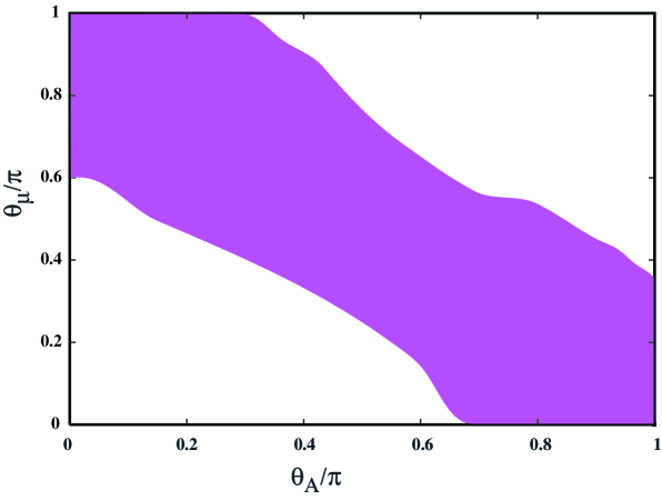
FIG. 1.: The allowed region in the $\theta_{A}$–$\theta_{\mu}$ plane with LO for $10\leq\tan\beta\leq 60$. The allowed region when BLO Wilson coefficients are included is similar.

In Figure 2, we show the variation of the CP asymmetry with $\tan\beta$ for LO (upper window) and BLO (lower window) Wilson coefficients. The individual points correspond to a scan over values of $\theta_{\mu}$ and $\theta_{A}$ taken from Figure 1. Since the allowed values of the phases in the LO and BLO approximations are not the same, the surviving points in the scans will also differ as seen in comparing the two panels of Figure 2. At LO precision, $\mbox{A}_{\mbox{CP}}$ ranges from $-8\%$ to $8\%$ uniformly, that is, for a given value of $\tan\beta$, there is no strong preference to positive or negative values. When BLO Wilson coefficients are included however, the dependence of the CP asymmetry is modified. We find that there is an observable preference to to positive values of $\mbox{A}_{\mbox{CP}}$ distorting the uniformity of the LO behavior. This particular behaviour of the CP asymmetry results from our choice of a positive gluino mass, $\theta_{\widetilde{g}}=0$. For $\theta_{\widetilde{g}}=\pi$, the graph is approximately inverted (relative to that shown in the lower panel of Figure 2), i.e., with a preference to negative values. Therefore, the sign of the CP asymmetry tracks the phase of the gluino mass for most of the parameter space at large values of $\tan\beta$.

FIG. 2.: Variation of the CP asymmetry with $\tan\beta$ for LO (upper window) and BLO (lower window) Wilson coefficients for $10\leq\tan\beta\leq 60$, and $0\leq(\theta_{\mu},\theta_{A})\leq\pi$. Individual points correspond to values of the two CP violating phases taken from Figure 1. For $\tan\beta\mathrel{\raise 1.29167pt\hbox{$<$\kern-7.5pt\lower 4.30554pt\hbox{$\sim$}}}35$, for which the radiative corrections are small, both asymmetries behave similarly, and fall around $2\%$ when $\tan\beta\sim 10$. The BLO CP asymmetry shown here is computed for a positive gluino mass, and to a good approximation, $\mbox{A}_{\mbox{CP}}\rightarrow-\mbox{A}_{\mbox{CP}}$ as $m_{\widetilde{g}}\rightarrow-m_{\widetilde{g}}$ at large $\tan\beta$.

In general, there are two main reasons that the CP asymmetry is enhanced: ($i$) it is maximized when the branching ratio is minimized, and ($ii$) it can be maximized due to specific relations among the Wilson coefficients depending on the underlying model. Indeed, it is known that the asymmetry in the decay behaves as $\sim 10\%\times\left|{\cal{C}}_{8}(m_{b})\right|/\left|{\cal{C}}_{7}(m_{b})\right|$ [13, 37], and reaches the $10\%$ level when the chromoelectric coefficient has a size similar to the electric coefficient, as was first pointed out in the framework of two–doublet models [37]. Depicted in Figure 3 is the variation of the CP asymmetry with the branching ratio of the decay, where the enhancement of the asymmetry with decreasing branching ratio is manifest. In this figure, we assume $m_{\widetilde{g}}>0$. For most of the points plotted, there is a correlation between the signs of the CP asymmetry and the gluino mass.

FIG. 3.: Variation of the CP asymmetry with the branching ratio using BLO Wilson coefficients for $m_{\widetilde{g}}>0$. For most of the points shown, the sign of the CP asymmetry is correlated to the sign of the gluino mass.

In this section we have analyzed the rare radiative $B$ meson decay $B\rightarrow X_{s}\gamma$ in the framework of an effective supersymmetric model [18] in which the sfermions in first two generations are heavy enough to suppress the one–loop EDMs [4, 5, 7, 8], and the two–loop EDMs [19] are suppressed by appropriately tuning the stop and sbottom sector parameters in addition to choosing small stop mixing angles (which are also required by the electroweak precision data).

In this framework we find that, in regions of the SUSY parameter space where there is a large CP asymmetry at LO, the BLO effects induce asymmetries which are twice as large as the LO asymmetry at sufficiently large values of $\tan\beta$. Moreover, certain combinations of the SUSY soft phases are constrained to reside close to CP–conserving points in order to agree with experimental bounds. The size of the allowed ranges of the SUSY phases, which is mainly dictated by the experimental bounds on the branching fraction and the EDMs, is wide enough to have an enhanced production of the P–wave bottomonia in lepton colliders [10], to have observable CP violation in the Higgs system [3] in next generation of colliders, and to have observable leptonic polarization asymmetries in $B$–meson decays [9]. Neither of these phenomena have been observed yet but they are all interrelated. First of all, the P–wave bottomonium production rate is determined by $\mbox{Im}[{\cal{C}}_{7}]$ [10] which has a richer structure in the BLO case. Secondly, in the Higgs system, where the mixing of the opposite CP Higgs bosons depend on $\sin(\theta_{2})\sin(\theta_{\widetilde{t}})$, there exists sizable CP violation in the parameter space of Fig. 1 when $\theta_{2}$ differs from $\pi$. Moreoever, altough $\theta_{\widetilde{t}}$ is relatively small (as required by the precision data and EDM constraints) the CP–violating Higgs mixings are still important with relatively light Higgs bosons [3] as allowed by $b\rightarrow s\gamma$. Finally, a simultaneous measurement of the lepton polarization asymmetry and CP asymmetry in $B\rightarrow K^{\star}\ell^{+}\ell^{-}$ decay provides a good consistencey check of the ’new physics’ contributions where both depend on the imaginary parts of the dipole coefficients ${\cal{C}}_{7,8}$ (and other relevant coefficients), and they are necessarily enhanced in the BLO case [9].

IV $B\rightarrow X_{s}\gamma$ in the CMSSM

In this section, we will analyze the implications of the SUSY CP violating phases on $b\rightarrow s\gamma$ in the framework of the minimal supergravity model, or equivalently, the constrained MSSM or CMSSM [38]. In the CMSSM, universal gaugino masses $m_{1/2}$, scalar masses $m_{0}$ (including those of the Higgs multiplets) and trilinear supersymmetry breaking parameters $A_{0}$ are input at the supersymmetric grand unification scale. In this framework, the Higgs mixing parameter $\mu$ can be derived (up to its phase which does not run) from the other MSSM parameters by imposing the electroweak vacuum conditions for any given value of $\tan\beta$. In the CMSSM, there are only two physical phases to consider. Thus, given the set of input parameters determined by $\{m_{1/2},m_{0},|A_{0}|,\tan\beta,\theta_{\mu}$ and $\theta_{A}\}$, the entire spectrum of sparticles can be derived.

In CMSSM, the low energy mass spectrum is completely controlled by the GUT–scale parameters above, and one cannot decouple the first two generations of sfermions (though they are nearly degenerate to an excellent approximation); therefore, the Wilson coefficients at the SUSY–breaking scale (18) must be updated by taking $Q_{12}\sim Q_{s}$. Consequently, the contribution of squarks in the first two generations give

$${\cal{C}}_{7,8}^{\chi}(Q_{s}) = \left[{\cal{C}}_{7,8}^{\chi}(Q_{s})\ \mbox{in Eq.}\ (\ref{wilson})\right]$$ (34)

$$+ \sum_{j=1}^{2}\Bigg{\{}\left|\widehat{\Gamma}_{L}^{1j}\right|^{2}\ \frac{M_{W}^{2}}{Q_{s}^{2}}\ F_{7,8}^{LL}\left[\frac{Q_{s}^{2}}{M_{\chi^{\pm}_{j}}^{2}}\right]+\left(\widehat{\Gamma}_{L}^{1j}\right)^{\star}\ \widehat{\Gamma}_{R}^{1j}\ \frac{M_{W}}{M_{\chi^{\pm}_{j}}}\ F_{7,8}^{LR}\left[\frac{Q_{s}^{2}}{M_{\chi^{\pm}_{j}}^{2}}\right]\Bigg{\}}$$ (35)

where $\widehat{\Gamma}_{L,R}$ is obtained by replacing the stop mixing matrix $C_{\widetilde{t}}$ with the identity matrix in (19). If the CMSSM spectrum admits the lighter stop to be as light as $\sim Q_{W}$ (which can occur when large values of $A_{0}$ are assumed), then the analysis of $b\rightarrow s\gamma$ proceeds as in the last section, in particular, the chargino contribution at the weak scale is given by (25) and (27) where ${\cal{C}}_{7,8}^{\chi}(Q_{s})$ is now given by (34).

The remaining colored sparticles typically have masses around the SUSY breaking scale, $Q_{s}$. For such a hierarchy of the masses, the analysis of the Wilson coefficients differs from the previous cases, in particular, the chargino contribution at the SUSY breaking scale is now given by

$${\cal{C}}_{7,8}^{\chi}(Q_{s}) = \sum_{j=1}^{2}\Bigg{\{}\left|\widehat{\Gamma}_{L}^{1j}\right|^{2}\ \frac{M_{W}^{2}}{Q_{s}^{2}}\ F_{7,8}^{LL}\left[\frac{Q_{s}^{2}}{M_{\chi^{\pm}_{j}}^{2}}\right]+\left(\widehat{\Gamma}_{L}^{1j}\right)^{\star}\ \widehat{\Gamma}_{R}^{1j}\ \frac{M_{W}}{M_{\chi^{\pm}_{j}}}\ F_{7,8}^{LR}\left[\frac{Q_{s}^{2}}{M_{\chi^{\pm}_{j}}^{2}}\right]$$ (36)

$$- \sum_{k=1}^{2}\left\{\left|\Gamma_{L}^{kj}\right|^{2}\ \frac{M_{W}^{2}}{M^{2}_{\tilde{t}_{k}}}\ F_{7,8}^{LL}\left[\frac{M^{2}_{\tilde{t}_{k}}}{M_{\chi^{\pm}_{j}}^{2}}\right]-\gamma^{kj}_{LR}\ \frac{M_{W}}{M_{\chi^{\pm}_{j}}}\ F_{7,8}^{LR}\left[\frac{M^{2}_{\tilde{t}_{k}}}{M_{\chi^{\pm}_{j}}^{2}}\right]\right\}\Bigg{\}}$$ (37)

which can be rescaled to the electroweak scale via QCD running

$${\cal{C}}_{7}^{\chi}(Q_{W}) = \left(\frac{\alpha_{s}(Q_{s})}{\alpha_{s}(Q_{W})}\right)^{\frac{16}{3\beta_{0}}}{\cal{C}}_{7}^{\chi}(Q_{s})+\frac{8}{3}\left[\left(\frac{\alpha_{s}(Q_{s})}{\alpha_{s}(Q_{W})}\right)^{\frac{14}{3\beta_{0}}}-\left(\frac{\alpha_{s}(Q_{s})}{\alpha_{s}(Q_{W})}\right)^{\frac{16}{3\beta_{0}}}\right]{\cal{C}}_{8}^{\chi}(Q_{s})$$ (38)

$${\cal{C}}_{8}^{\chi}(Q_{W}) = \left(\frac{\alpha_{s}(Q_{s})}{\alpha_{s}(Q_{W})}\right)^{\frac{14}{3\beta_{0}}}{\cal{C}}_{8}^{\chi}(Q_{s})$$ (39)

where $\beta_{0}=7$, as the colored spectrum below $Q_{s}$ is just that of the SM. The formulae (34,36) give possible changes in the effective theory at the weak scale in analyzing $b\rightarrow s\gamma$, which will be numerically analyzed by taking into account cosmological and collider constraints.

Due to the restricted parameter set, and the strong correlation among the masses of the sparticles, there are a number of experimental constraints which must be considered. The most important of these are provided by LEP searches for sparticles and Higgs bosons [39], the latter constraining the sparticle spectrum indirectly via radiative corrections. The kinematic reach for charginos was $m_{\chi^{\pm}}=104$ GeV, and the LEP limit is generally close to this value, within the CMSSM framework. The LEP searches for sleptons impose $m_{\tilde{e}}>97$ GeV, $m_{\tilde{\mu}}>94$ GeV and $m_{\tilde{\tau}}>80$ GeV for $m_{\chi}<80$ GeV. Other important sparticle constraints are those on stop squarks ${\tilde{t}}$: $m_{\tilde{t}}>94$ GeV for $m_{\chi}<80$ GeV from LEP, and $m_{\tilde{t}}\mathrel{\raise 1.29167pt\hbox{$>$\kern-7.5pt\lower 4.30554pt\hbox{$\sim$}}}115$ GeV for $m_{\chi}\mathrel{\raise 1.29167pt\hbox{$<$\kern-7.5pt\lower 4.30554pt\hbox{$\sim$}}}50$ GeV from the Fermilab Tevatron collider [40].

The lower limit on the mass of a Standard Model Higgs boson imposed by the combined LEP experiments is $113.5$ GeV [41]. This lower limit also applies to the MSSM for small $\tan\beta$, even if squark mixing is maximal. In the CMSSM, maximal mixing is not attained, and the $e^{+}e^{-}\to Z^{0}+h$ production rate is very similar to that in the Standard Model [42], for all values of $\tan\beta$. As is well known, a 2.9-$\sigma$ signal for a Higgs boson weighing about $115^{+1.3}_{-0.7}$ GeV has been reported [41].

In addition, the BNL E821 experiment has recently reported [43] a new value for the anomalous magnetic moment of the muon: $g_{\mu}-2\equiv 2\times a_{\mu}$, which yields an apparent discrepancy with the Standard Model prediction at the level of 2.6 $\sigma$: $\delta a_{\mu}\;=\;(43\pm 16)\times 10^{-10}.$ This result has been well studied in the CMSSM [44], resulting in a strong preference to $\mu>0$ and relatively low values of $m_{1/2}$ and $m_{0}$.

In addition to the phenomenological constraints, one must also carefully consider the resultant relic density of the LSP [45]. This constraint generally disfavors large values of either of the SUSY breaking mass scales $m_{0},m_{1/2}$ except in some well defined regions of parameter space where an enhanced annihilation cross section ensures that the relic density $\Omega h^{2}<0.3$ [46, 47]. These include regions where co-annihilations are important [48], s-channel pseudo-scalar exchange is important [46], or in the focus point region at large $m_{0}$ [49]. The co-annihilation region is important at large $m_{1/2}$ and the allowed regions due to pseudo-scalar exchange occur at large $m_{1/2}$ and large $m_{0}$ at large $\tan\beta$. As we will see, the sensitivity to the phase $\theta_{A}$ occurs at relatively low $m_{1/2}$ and $m_{0}$. This is the region favored by the recent results from the $g-2$ experiment.

In Figure 4, we show the cosmological and phenomenological constraints in the $m_{1/2},m_{0}$ parameter plane for $\tan\beta=10$. The very dark (red) regions correspond to either $m_{\tilde{\tau}_{1}}<m_{\chi}$, or $m_{\tilde{t}_{1}}<m_{\chi}$ where the subscript 1 denotes the lighter of the $\tilde{\tau}$ or $\tilde{t}$ mass eigenstates. These regions are ruled out by the requirement that the LSP be neutral. For $A_{0}<0$, the excluded region is found at low values of $m_{0}$ where $\tilde{\tau}_{1}$ is the LSP. For $A_{0}>0$, the $\tilde{\tau}_{1}$ LSP region is similar, but there is in addition a region where the stop is lighter than the neutralino at low $m_{1/2}$ and extends to $m_{0}\simeq 500$ GeV (in much of this region the stop is actually tachyonic). We show as (red) dash-dotted, nearly vertical lines the $m_{h}=113$ GeV contour calculated using FeynHiggs [50]. For $A_{0}<0$, the limit is quite strong and excludes values of $m_{1/2}\mathrel{\raise 1.29167pt\hbox{$<$\kern-7.5pt\lower 4.30554pt\hbox{$\sim$}}}440$ GeV. For $A_{0}>0$, the Higgs mass limit is not significant. The (dashed) bound on the chargino mass from LEP excludes very low values of $m_{1/2}\mathrel{\raise 1.29167pt\hbox{$<$\kern-7.5pt\lower 4.30554pt\hbox{$\sim$}}}140$ GeV. The branching ratio for $b\rightarrow s\gamma$ excludes a dark (green) shaded area at low $m_{1/2}$. For these parameter choices, this region is only present for $A_{0}>0$. The (pink) medium-shaded region corresponds to the region preferred by the recent $g-2$ experiment. The region bounded by the solid curves corresponds to the 2-$\sigma$ preferred region, whereas the dashed curves correspond to 1-$\sigma$. Finally, the (turquoise) light shaded region corresponds to the parameter space for which the neutralino relic density falls in the range $0.1<\Omega h^{2}<0.3$.

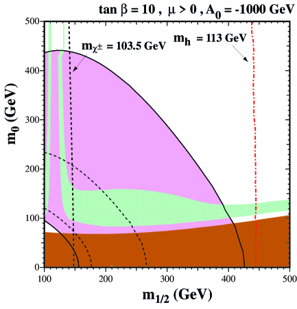
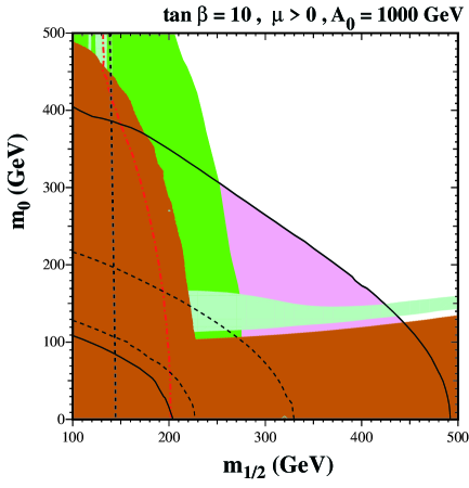
FIG. 4.: The $(m_{1/2},m_{0})$ planes for $\tan\beta=10$, $\mu>0$ and (a) $A_{0}=-1000$ GeV, (b) $A_{0}=1000$ GeV. In each case we have assumed $m_{t}=175$ and $m_{b}(m_{b})^{\overline{MS}}_{SM}=4.25$ GeV. The near-vertical (red) dot-dashed lines are the contours $m_{h}=113$ GeV, as evaluated using the FeynHiggs code. The medium (dark green) shaded regions are excluded by $b\rightarrow s\gamma$. The light (turquoise) shaded areas are the cosmologically preferred regions with $0.1\leq\Omega h^{2}\leq 0.3$. In the dark (brick red) shaded regions, the LSP is either ${\tilde{\tau}}_{1}$ or $\tilde{t}_{1}$, so this region is excluded. The regions allowed by the E821 measurement of $a_{\mu}$ at the 2-$\sigma$ level are shaded (pink) and bounded by solid black lines, with dashed lines indicating the 1-$\sigma$ ranges.

The CP violating phases in the CMSSM have been studied [6, 7, 8] in relation to their effects on EDMs. Generally, it is found that while the phase of $\mu$ is strongly constrained by the EDMS to be close to either of its two CP conserving values, the phase of $A$ is largely unconstrained. For this reason, in what follows, we will set $\theta_{\mu}=0$ and concentrate on the effect of $\theta_{A}$ on the rate for $b\rightarrow s\gamma$.

In the CMSSM, we specify the phases at the GUT scale. Since $\theta_{\mu}$, is not affected by the running of the renormalization group equations, the value of $\theta_{\mu}$ at the weak scale is identical to its input value. However, the real and imaginary parts of $A$ run differently and hence, the weak scale phase, $\theta_{A}$ differs from its input value $\theta_{A_{0}}$. In Figure 5, we show the resulting phase of $A_{t}$ at the weak scale as a function of the input value for several choices of $m_{1/2}=200,400$, and 600 GeV, with $m_{0}$ = 400 GeV and $|A_{0}|=1000$ GeV. The shaded regions show the dependence with respect to $\tan\beta$ between 10 and 30. The values of $\theta_{A}$ for $\tan\beta=10$ are given by the lower edge of each shaded region, whereas the result for $\tan\beta=30$ is given by the upper edge. As one can see in the figure, the tendency of the RGE’s is to drive $A_{t}$ towards real values, particularly at higher values of $m_{1/2}$. Nevertheless, the resulting phase at the weak scale is sufficient to have a strong impact on the branching ratio of $b\rightarrow s\gamma$ as we now discuss.

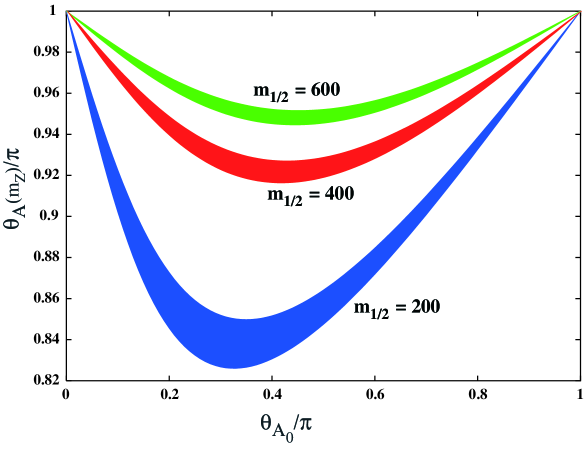
FIG. 5.: The value of the phase of A at the weak scale as a function of the input phase, $\theta_{A_{0}}$ for $m_{1/2}$ = 200, 400, and 600 GeV in the range $\tan\beta=$ 10 - 30. Here $m_{0}$ is fixed at 400 GeV and $|A_{0}|=1000$ GeV.

In Figures 6 – 8, we show the calculated branching ratio of $B\rightarrow X_{s}\gamma$ (scaled to the experimental value of $3.11\times 10^{-4}$) as a function of $m_{1/2}$ for $\theta_{A_{0}}=0,\pi/2$, and $\pi$ for both $\mu<0$ (dotted curves) and $\mu>0$ (dashed curves). The horizontal lines correspond to the 95 % CL range (2.27 – 4.01) $\times 10^{-4}$. We have fixed the value of $m_{0}=140$, for $\tan\beta=10$, which is the value which best yields a good relic density (for this value of $|A_{0}|$). As one can see the curves calculated for $\mu<0$ show a branching ratio which is too large unless $m_{1/2}\mathrel{\raise 1.29167pt\hbox{$>$\kern-7.5pt\lower 4.30554pt\hbox{$\sim$}}}430$ GeV. At low $m_{1/2}$, even though the phase of $A_{0}$ has a strong effect on the calculated branching ratio, it can not reduce it to the experimentally allowed value. On the other hand, for $\mu>0$, we see that while all values of $m_{1/2}$ are allowed by $b\rightarrow s\gamma$ for $\theta_{A_{0}}=\pi$, there is a strong dependence on $\theta_{A}$ thus enabling one to set a limit on the phase of $A_{0}$ from $b\rightarrow s\gamma$, at least for some values of $m_{1/2}$. One should bear in mind that while the range $m_{1/2}<440$ GeV is nominally excluded by the Higgs mass limit, the theoretical uncertainty in the calculated Higgs mass is about 3 GeV. The $m_{h}=110$ GeV contour would lie at $m_{1/2}=320$ GeV in Figure 4b.

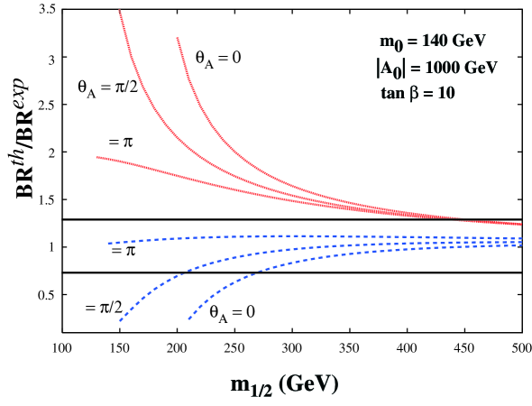
FIG. 6.: The calculated branching ratio for $b\to s\gamma$ scaled to the experimental value of 3.11 $\times 10^{-4}$ as a function of $m_{1/2}$ for $\tan\beta=10,m_{0}=140$ GeV, and $|A_{0}|=1000$ GeV. Shown are the branching ratios for $\theta_{A_{0}}=0,\pi/2$, and $\pi$. Curves for $\mu>0$ are shown as dotted and red, while curves for $\mu<0$ are dashed and blue. The horizontal solid black lines delimit the 95 % CL experimental range.

In Figures 7 and 8, we show the analogous behavior of the branching ratio for $\tan\beta=20$ and 30 respectively. For the larger values of $\tan\beta$, it is not possible to satisfy the cosmological constraint with a single value of $m_{0}$. However, we have chosen a value of $m_{0}$ which best fits the cosmological region for both signs of $\mu$ and $A$. In addition, we note that the dependence of the branching ratio on $m_{0}$ is relatively weak. Thus had we in fact varied $m_{0}$ with $m_{1/2}$ (to insure a proper relic density), the curves in Figures 7 and 8 would differ only very slightly.

The sensitivity of the branching ratio to the phase of $A_{0}$ is also strong at the larger values of $\tan\beta$ as seen in Figures 7 and 8. As $\tan\beta$ is increased, one is pushed to higher values of $m_{1/2}$ and therefore we are able to set bounds on $\theta_{A_{0}}$ for a wider range in $m_{1/2}$. The Higgs mass bounds are also weaker at higher $\tan\beta$.

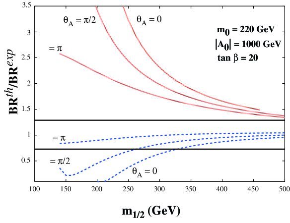
FIG. 7.: As in Fig. 6 for $\tan\beta=20$ and $m_{0}=220$

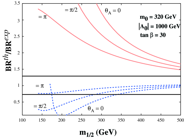
FIG. 8.: As in Fig. 6 for $\tan\beta=30$ and $m_{0}=320$

As noted above, for a given range in $m_{1/2}$, we are able to use the constraints from $b\to s\gamma$ to set a limit on $\theta_{A_{0}}$. These limits are summarized in Figure 9. Shown there is the lower limit to $\theta_{A_{0}}$ as a function of $m_{1/2}$ for the three values of $\tan\beta$ indicated. Values of $m_{0}$ were taken from Figures 6 - 8. One can also read off from this figure the minimal value of $m_{1/2}$ such that all values of the phase, $\theta_{A_{0}}$, are allowed.

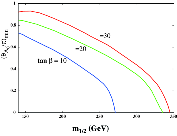
FIG. 9.: The lower bound on $\theta_{A_{0}}$ as a function of $m_{1/2}$ for $\tan\beta=10,20$ and 30. Values of $m_{0}$ are the same as in Figures 6 - 8. Note that at $m_{1/2}\approx 170\ {\rm GeV}$ there will be a small window at $\theta_{A_{0}}\approx 0$ which is allowed for $\tan\beta=30$. We do not include this curve in the figure.

Finally, in Figures 10 and 11, we show the branching ratio as a function of $\tan\beta$ for fixed $m_{0}=400$ GeV , $|A_{0}|$ = 1000 GeV, and $m_{1/2}$ = 200 and 400 GeV respectively. Recall that the sensitivity of these curves to $m_{0}$ (at least for relatively low $m_{0}$) is rather small. As one can see, at small values of $m_{1/2}$, there is a strong dependence of the branching ratio on the phase. At higher values of $m_{1/2}$, not only is the dependence weaker, but also as one can see, for a given value of $\tan\beta$, either all phases are allowed or forbidden by the experimental constraint on $b\to s\gamma$.

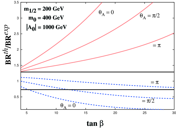
FIG. 10.: The calculated branching ratio for $b\to s\gamma$ scaled to the experimental value of 3.11 $\times 10^{-4}$ as a function of $\tan\beta$ for $m_{1/2}=200$ GeV, $m_{0}=400$ GeV, and $|A_{0}|=1000$ GeV. Shown are the branching ratios for $\theta_{A_{0}}=0,\pi/2$, and $\pi$. Curves for $\mu>0$ are shown as dotted and red, while curves for $\mu<0$ are dashed and blue. The horizontal solid black lines delimit the 95 % CL experimental range.

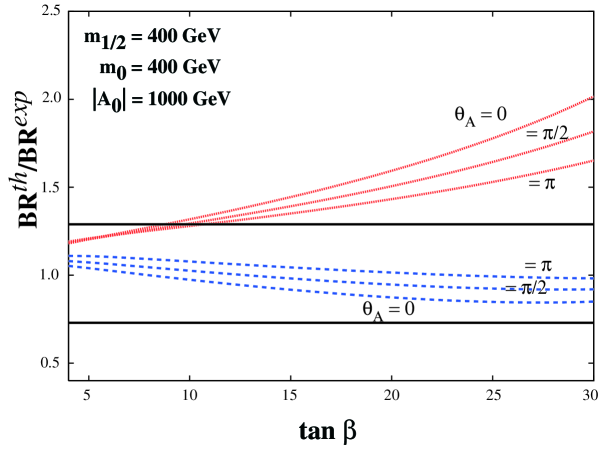
FIG. 11.: As in Fig. 10 for $m_{1/2}=400$.

V Summary

In this work we have performed a thorough study of the constraints on the SUSY soft phases from $B\to X_{s}\gamma$ decay using existing experimental bounds. Our analysis was restricted to the MFV scheme in which flavor violation occurs only through the CKM matrix. We considered both unconstrained as well as constrained supersymmetric models.

In particular, we considered an unconstrained supersymmetric model, for which low energy supersymmetry bears no imprint of the stringy boundary conditions at ultra high energies. In particular, we chose a particle spectrum such that the charged Higgs boson, charginos, and the lighter stop are relatively light (with masses of order the weak scale). In this case, we found that: ($i$) the sum of the phases of the $\mu$ parameter and the stop trilinear coupling must take values around the CP–conserving point $\pi$, with a width determined by experimental uncertainties; ($ii$) the sum of the phases of the $\mu$ parameter and the gluino mass tends to zero within the present experimental precision; ($iii$) the LO CP asymmetry swings from $-8\%$ to $+8\%$ where positive and negative values are equally possible; ($iv$) the inclusion of the $\tan\beta$–enhanced corrections widens the allowed range of $\tan\beta$ values, though it does not lead to a significant change in the size of the CP asymmetry except for the fact that ($a$) it can be approximately twice as large as the LO prediction, and ($b$) it tends to follow the sign of the gluino mass for most of the parameter space, for $\tan\beta\sim{\cal{O}}(50)$. Consequently, there exist observable effects of the SUSY threshold corrections at large $\tan\beta$. If experiments measure a large CP asymmetry (compared to the SM expectation), this may be interpreted as having originating from the soft phases and as an indication for weak scale SUSY.

After analyzing the implications of the CP violating phases in an unconstrained supersymmetric model, we turned to a detailed discussion of the CMSSM with explicit CP violation. In our numerical estimates, we took the $\mu$ parameter to be real as implied by earlier studies of the EDM constraints, and we explored the $b\rightarrow s\gamma$ branching ratio in regions of the parameter space allowed by the cosmological as well as other collider constraints displayed in Figure 4. In particular, we discussed the impact of the phase of the universal trilinear coupling at the GUT scale on the branching ratio. As the associated figures suggest, the branching ratio is quite sensitive to $\theta_{A_{0}}$, at least for moderately small values of $m_{1/2}$. As we have shown, for positive values of $\mu$, while $\theta_{A_{0}}=\pi$, generally produced branching ratios in agreement with the experimental bounds, deviations from this CP conserving point can lead to branching ratios which are not compatible with experiment. We have also seen that the phase of the universal trilinear coupling can not ameliorate the inconsistency at low $m_{1/2}$ when $\mu<0$.

Acknowledgments
This work was supported in part by DOE grant DE–FG02–94ER–40823. We would like to thank Toby Falk, Gerri Ganis and Stefano Rigolin for many helpful conversations.

Appendix A: Masses and Mixings of SUSY Particles

Given that the intergenerational mixings are proportional to the corresponding quark masses, the weak eigenstate squarks are approximately the mass eigenstates for the first two generations. However, the third generation squarks as well as the gauginos and Higgsinos can mix strongly after electroweak symmetry breaking. Since the chargino mass matrix $M_{\chi^{\pm}}$ is not hermitian, it is convenient to consider $\widetilde{M_{L}}^{2}=M_{\chi^{\pm}}^{\dagger}\cdot M_{\chi^{\pm}}$ and $\widetilde{M_{R}}^{2}=M_{\chi^{\pm}}\cdot M_{\chi^{\pm}}^{\dagger}$ which are hermitian and can be diagonalized by

$${C}_{\alpha}^{\dagger}\,\widetilde{M_{\alpha}}^{2}\,{C}_{\alpha}=\mbox{diag.}\left(M^{2}_{\alpha_{1}},M^{2}_{\alpha_{2}}\right)\>\>\mbox{with}\>\>{C}_{\alpha}=\left(\begin{array}[]{cc}\cos\theta_{\alpha}&-\sin\theta_{\alpha}\,e^{-i\gamma_{\alpha}}\\ \sin\theta_{\alpha}\,e^{i\gamma_{\alpha}}&\cos\theta_{\alpha}\end{array}\right)\cdot\left(\begin{array}[]{cc}e^{i\eta_{\alpha}}&0\\ 0&e^{i\rho_{\alpha}}\end{array}\right)$$ (A.5)

The squark mass matrices $\widetilde{M_{\widetilde{t,b}}}^{2}$ are similarly diagonalized. The relative sign between $A_{t,b}$ and $\mu$ is set by the corresponding off–diagonal element of the sfermion mass matrix: $m^{2}_{12}=-m_{t}(A_{t}-\mu\cot\beta)$ for stops, and $m^{2}_{12}=-m_{b}(A_{b}-\mu\tan\beta)$ for sbottoms. In eq. (A.5), the explicit expressions for the angle parameters are given by

$$\gamma_{\widetilde{t}}=-\mbox{Arg}\left[A^{*}_{t}-\mu\cot\beta\right]\>\>,\>\>\tan\ 2\theta_{\widetilde{t}}=\frac{2m_{t}\left|A^{*}_{t}-\mu\cot\beta\right|}{M^{2}_{\tilde{t}_{L}}-M^{2}_{\tilde{t}_{R}}-(1/6)\cos 2\beta\left(5M_{Z}^{2}-8M_{W}^{2}\right)}$$ (A.6)

$$\gamma_{\widetilde{b}}=-\mbox{Arg}\left[A^{*}_{b}-\mu\tan\beta\right]\>\>,\>\>\tan\ 2\theta_{\widetilde{b}}=\frac{2m_{b}\left|A^{*}_{b}-\mu\tan\beta\right|}{M^{2}_{\tilde{b}_{L}}-M^{2}_{\tilde{b}_{R}}+(1/6)\cos 2\beta\left(M_{Z}^{2}-4M_{W}^{2}\right)}$$ (A.7)

$$\gamma_{L}=-\mbox{Arg}\left[M_{2}+\mu\cot\beta\right]\>\>,\>\>\tan\ 2\theta_{L}=\frac{\sqrt{8}M_{W}\sin\beta\left|M_{2}+\mu\cot\beta\right|}{M_{2}^{2}+|\mu|^{2}+2M_{W}^{2}\cos 2\beta}$$ (A.8)

$$\gamma_{R}=-\mbox{Arg}\left[M_{2}+\mu^{*}\tan\beta\right]\>\>,\>\>\tan\ 2\theta_{R}=\frac{\sqrt{8}M_{W}\cos\beta\left|M_{2}+\mu^{*}\tan\beta\right|}{M_{2}^{2}-\left|\mu\right|^{2}-2M_{W}^{2}\cos 2\beta}$$ (A.9)

where $0\leq\theta_{\alpha}\leq\pi/2$ to ensure $M^{2}_{\alpha_{1}}>M^{2}_{\alpha_{2}}$. Finally, one can choose $\eta_{\widetilde{t},L}=\rho_{\widetilde{t},L}=0$, and

$$\eta_{R} = \mbox{Arg}\left[c_{R}\left(M_{2}c_{L}+\sqrt{2}M_{W}\sin\beta s_{L}e^{i\gamma_{L}}\right)+s_{R}e^{-i\gamma_{R}}\left(\sqrt{2}M_{W}\cos\beta c_{L}+\mu s_{L}e^{i\gamma_{L}}\right)\right]$$ (A.10)

$$\rho_{R} = \mbox{Arg}\left[c_{R}\left(-\sqrt{2}M_{W}\cos\beta s_{L}e^{-i\gamma_{L}}-\mu c_{L}\right)-s_{R}e^{i\gamma_{R}}\left(-M_{2}s_{L}e^{-i\gamma_{L}}+\sqrt{2}M_{W}\sin\beta c_{L}\right)\right]$$ (A.11)

with $s_{L,R}=\sin\theta_{L,R}$ and $c_{L,R}=\cos\theta_{L,R}$. The mixing matrix $C_{\alpha}$ guarantees that both chargino masses are real positive with $M^{2}_{\chi_{1}}>M^{2}_{\chi_{2}}$ and $M^{2}_{\widetilde{t,b}_{1}}>M^{2}_{\widetilde{t,b}_{2}}$.

Finally, the neutralinos are described by a $4\times 4$ mass matrix

$$M^{0}\ =\ \left(\begin{array}[]{cccc}M_{1}&0&M_{Z}s_{w}\cos\beta&-M_{Z}s_{w}\sin\beta\\ 0&M_{2}&-M_{Z}c_{w}\cos\beta&M_{Z}c_{w}\sin\beta\\ M_{Z}s_{w}\cos\beta&-M_{Z}c_{w}\cos\beta&0&-\mu\\ -M_{Z}s_{w}\sin\beta&M_{Z}c_{w}\sin\beta&-\mu&0\end{array}\right)$$ (A.16)

which can be diagonalized numerically via

$$C_{0}^{T}M^{0}C_{0}=\mbox{diag.}\left(M_{\chi^{0}_{1}},\cdots,M_{\chi^{0}_{4}}\right)$$ (A.17)

where $M_{\chi^{0}_{1}}<\cdots<M_{\chi^{0}_{4}}$.

Appendix B: Loop Functions

The two–point function entering the expressions of $\epsilon_{bb,ts,tb}$ (11) is

$${\cal{H}}\left[x,y\right] = \frac{x}{(1-x)\ (x-y)}\ \ln{x}+\frac{y}{(1-y)\ (y-x)}\ \ln{y}$$ (B.1)

with ${\cal{H}}\left[1,1\right]=-1/2$, and ${\cal{H}}\left[1,0\right]=-1$.

The loop functions entering the expressions of the Wilson coefficients (16–18) are given by

$$F_{7}^{LL}\left[x\right] = \frac{x\left(7-5x-8x^{2}\right)}{36(x-1)^{3}}+\frac{x^{2}\left(3x-2\right)}{6(x-1)^{4}}\ln{x}$$ (B.2)

$$F_{7}^{LR}\left[x\right] = \frac{5-7x}{6(x-1)^{2}}+\frac{x\left(3x-2\right)}{3(x-1)^{3}}\ln{x}$$ (B.3)

$$F_{8}^{LL}\left[x\right] = \frac{x\left(2+5x-x^{2}\right)}{12(x-1)^{3}}-\frac{3x^{2}}{6(x-1)^{4}}\ln{x}$$ (B.4)

$$F_{8}^{LR}\left[x\right] = \frac{1+x}{2(x-1)^{2}}-\frac{x}{(x-1)^{3}}\ln{x}$$ (B.5)

$$\tilde{F}_{7}^{LL}\left[x\right] = \frac{x\left(3-5x\right)}{12(x-1)^{2}}+\frac{x\left(3x-2\right)}{6(x-1)^{3}}\ln{x}$$ (B.6)

$$\tilde{F}_{8}^{LL}\left[x\right] = \frac{x\left(3-x\right)}{4(x-1)^{2}}-\frac{x}{2(x-1)^{3}}\ln{x}\>.$$ (B.7)

In order to make numerical estimates, it is useful to know the values of these functions evaluated at $x=1$:

$$F_{7}^{LL}\left[1\right] = -\frac{5}{72}\>\>,\>\>F_{8}^{LL}\left[1\right]=-\frac{1}{24}\>\>,\>\>F_{7}^{LR}\left[1\right]=\frac{4}{9}\>\>,$$ (B.8)

$$F_{8}^{LR}\left[1\right] = \frac{1}{6}\>\>,\>\>\tilde{F}_{7}^{LL}\left[1\right]=-\frac{7}{36}\>\>,\>\>\tilde{F}_{8}^{LL}\left[1\right]=-\frac{1}{6}\>.$$ (B.9)

The two–loop EDMs, on the other hand, depend on the two–loop function

$$F\left[x\right]=\int_{0}^{1}dz\ \frac{z\overline{z}}{x-z\overline{z}}\ \ln{\frac{z\overline{z}}{x}}$$ (B.10)

where $\overline{z}=1-z$ with $F\left[1\right]\approx-2.34$.

REFERENCES

- [1] M. Dugan, B. Grinstein and L. Hall, Nucl. Phys. B255, 413 (1985); M. J. Duncan, Nucl. Phys. B221, 285 (1983).
- [2] B. A. Campbell, Phys. Rev. D 28 (1983) 209; J. S. Hagelin, S. Kelley and T. Tanaka, Nucl. Phys. B 415, 293 (1994); F. Gabbiani, E. Gabrielli, A. Masiero and L. Silvestrini, Nucl. Phys. B477, 321 (1996) [hep-ph/9604387].
- [3] A. Pilaftsis, Phys. Lett. B 435, 88 (1998) [hep-ph/9805373]; D. A. Demir, Phys. Rev. D 60, 055006 (1999) [hep-ph/9901389]; A. Pilaftsis and C. E. Wagner, Nucl. Phys. B 553, 3 (1999) [hep-ph/9902371]; T. Ibrahim and P. Nath, Phys. Rev. D 63, 035009 (2001) [hep-ph/0008237]; M. Carena, J. Ellis, A. Pilaftsis and C. E. Wagner, Nucl. Phys. B 586, 92 (2000) [hep-ph/0003180]; Phys. Lett. B 495, 155 (2000) [hep-ph/0009212].
- [4] R. Arnowitt, J.L. Lopez and D.V. Nanopoulos, Phys. Rev. D42 (1990) 2423; R. Arnowitt, M.J. Duff and K.S. Stelle, Phys. Rev. D43 (1991) 3085; P. Nath, Phys. Rev. Lett. 66 (1991) 2565; T. Falk, K.A. Olive and M. Srednicki, Phys.Lett. B354 (1995) 99. T. Ibrahim and P. Nath, Phys. Lett. B418 (1998) 98; T. Ibrahim and P. Nath, Phys. Rev. D57 (1998) 478. T. Ibrahim and P. Nath, Phys. Rev. D 58, 111301 (1998) [hep-ph/9807501]; T. Ibrahim and P. Nath, Phys. Rev. D61 (2000) 093004. M. Brhlik, G. J. Good and G. L. Kane, Phys. Rev. D 59, 115004 (1999) [hep-ph/9810457]; S. Pokorski, J. Rosiek and C. A. Savoy, Nucl. Phys. B 570, 81 (2000) [hep-ph/9906206].
- [5] Y. Kizukuri and N. Oshimo, Phys. Rev. D45 (1992) 1806; D46 (1992) 3025.
- [6] T. Falk and K. A. Olive, Phys. Lett. B375, 196 (1996) [hep-ph/9602299]; Phys. Lett. B 439, 71 (1998) [hep-ph/9806236]; C. Hamzaoui, M. Pospelov and R. Roiban, Phys. Rev. D 56, 4295 (1997) [hep-ph/9702292]; A. Bartl, T. Gajdosik, W. Porod, P. Stockinger and H. Stremnitzer, Phys. Rev. D 60, 073003 (1999) [hep-ph/9903402].
- [7] T. Falk, K. A. Olive, M. Pospelov and R. Roiban, Nucl. Phys. B 560, 3 (1999) [hep-ph/9904393]; V. Barger, T. Falk, T. Han, J. Jiang, T. Li and T. Plehn, hep-ph/0101106.
- [8] S. Abel, S. Khalil and O. Lebedev, hep-ph/0103320.
- [9] F. Kruger and J. C. Romao, Phys. Rev. D 62, 034020 (2000) [hep-ph/0002089]; T. M. Aliev, D. A. Demir and M. Savci, Phys. Rev. D 62, 074016 (2000) [hep-ph/9912525].
- [10] D. A. Demir and M. B. Voloshin, Phys. Rev. D 63, 115011 (2001) [hep-ph/0012123].
- [11] A. Ali, H. Asatrian and C. Greub, Phys. Lett. B429, 87 (1998) [hep-ph/9803314].
- [12] A. Ali and E. Lunghi, hep-ph/0105200.
- [13] A. L. Kagan and M. Neubert, Phys. Rev. D 58, 094012 (1998) [hep-ph/9803368].
- [14] T. Nihei, Prog. Theor. Phys. 98, 1157 (1997) [hep-ph/9707336]; S. Baek and P. Ko, Phys. Rev. Lett. 83, 488 (1999) [hep-ph/9812229]; D. A. Demir, A. Masiero and O. Vives, Phys. Rev. Lett. 82, 2447 (1999) [hep-ph/9812337].
- [15] K. F. Smith et al., Phys. Lett. B 234, 191 (1990); I. S. Altarev et al., Phys. Lett. B 276, 242 (1992); P. G. Harris et al., Phys. Rev. Lett. 82, 904 (1999).
- [16] E. D. Commins, S. B. Ross, D. DeMille and B. C. Regan, Phys. Rev. A 50, 2960 (1994).
- [17] J.P. Jacobs et al., Phys. Rev. Lett. 71 (1993) 3782; J.P. Jacobs et al., Phys. Rev. A52 (1995) 3521; M. V. Romalis, W. C. Griffith and E. N. Fortson, Phys. Rev. Lett. 86, 2505 (2001) [hep-ex/0012001].
- [18] A. G. Cohen, D. B. Kaplan and A. E. Nelson, Phys. Lett. B 388, 588 (1996) [hep-ph/9607394].
- [19] D. Chang, W. Keung and A. Pilaftsis, Phys. Rev. Lett. 82, 900 (1999) [hep-ph/9811202]; A. Pilaftsis, Phys. Lett. B471, 174 (1999) [hep-ph/9909485]; D. Chang, W. Chang and W. Keung, Phys. Lett. B478, 239 (2000) [hep-ph/9910465].
- [20] K. Chetyrkin, M. Misiak and M. Munz, Phys. Lett. B 400, 206 (1997) [Erratum-ibid. B 425, 414 (1997)] [hep-ph/9612313]; T. Hurth, hep-ph/0106050; C. Greub, T. Hurth and D. Wyler, Phys. Rev. D 54, 3350 (1996) [hep-ph/9603404]; K. Adel and Y. Yao, Phys. Rev. D 49, 4945 (1994) [hep-ph/9308349]; A. Ali and C. Greub, Phys. Lett. B 361, 146 (1995) [hep-ph/9506374].
- [21] M. Ciuchini, G. Degrassi, P. Gambino and G. F. Giudice, Nucl. Phys. B 527, 21 (1998) [hep-ph/9710335]; F. M. Borzumati and C. Greub, Phys. Rev. D 58, 074004 (1998) [hep-ph/9802391]; Phys. Rev. D 59, 057501 (1999) [hep-ph/9809438].
- [22] M. Ciuchini, G. Degrassi, P. Gambino and G. F. Giudice, Nucl. Phys. B534, 3 (1998) [hep-ph/9806308].
- [23] F. Borzumati, C. Greub, T. Hurth and D. Wyler, Phys. Rev. D 62, 075005 (2000) [hep-ph/9911245].
- [24] S. Ahmed et al. [CLEO Collaboration], hep-ex/9908022.
- [25] R. Barate et al. [ALEPH Collaboration], Phys. Lett. B 429, 169 (1998).
- [26] K. Abe et al. [Belle Collaboration], hep-ex/0103042.
- [27] A. L. Kagan and M. Neubert, Eur. Phys. J. C7, 5 (1999) [hep-ph/9805303].
- [28] T. E. Coan et al. [CLEO Collaboration], hep-ex/0010075.
- [29] J. Ellis, G. Ganis, D. V. Nanopoulos and K. A. Olive, Phys. Lett. B 502, 171 (2001) [hep-ph/0009355]; J. Ellis, T. Falk, G. Ganis, K. A. Olive and M. Srednicki, hep-ph/0102098.
- [30] D. M. Pierce, J. A. Bagger, K. Matchev and R. Zhang, Nucl. Phys. B491, 3 (1997) [hep-ph/9606211]; M. Carena, D. Garcia, U. Nierste and C. E. Wagner, Nucl. Phys. B577, 88 (2000) [hep-ph/9912516]; T. Blazek, S. Raby and S. Pokorski, Phys. Rev. D 52, 4151 (1995) [hep-ph/9504364]; H. E. Haber, M. J. Herrero, H. E. Logan, S. Penaranda, S. Rigolin and D. Temes, Phys. Rev. D 63, 055004 (2001) [hep-ph/0007006]; V. Barger, M. S. Berger, P. Ohmann and R. J. Phillips, Phys. Rev. D 51, 2438 (1995) [hep-ph/9407273].
- [31] G. Degrassi, P. Gambino and G. F. Giudice, JHEP0012, 009 (2000) [hep-ph/0009337].
- [32] S. Bertolini, F. Borzumati, A. Masiero and G. Ridolfi, Nucl. Phys. B353, 591 (1991); F. M. Borzumati, Z. Phys. C 63, 291 (1994) [hep-ph/9310212]; R. Barbieri and G. F. Giudice, Phys. Lett. B 309, 86 (1993) [hep-ph/9303270]; N. Oshimo, Nucl. Phys. B 404, 20 (1993); M. A. Diaz, Phys. Lett. B 304, 278 (1993) [hep-ph/9303280]; Y. Okada, Phys. Lett. B 315, 119 (1993) [hep-ph/9307249]; R. Garisto and J. N. Ng, Phys. Lett. B 315, 372 (1993) [hep-ph/9307301];
- [33] H. Baer, M. Brhlik, D. Castano and X. Tata, Phys. Rev. D 58, 015007 (1998) [hep-ph/9712305]; W. d. Boer, M. Huber, A. V. Gladyshev and D. I. Kazakov, hep-ph/0102163.
- [34] M. Carena, D. Garcia, U. Nierste and C. E. Wagner, hep-ph/0010003.
- [35] T. Goto, Y. Y. Keum, T. Nihei, Y. Okada and Y. Shimizu, Phys. Lett. B460, 333 (1999) [hep-ph/9812369]; D. A. Demir, A. Masiero and O. Vives, Phys. Rev. D 61, 075009 (2000) [hep-ph/9909325]; Phys. Lett. B 479, 230 (2000) [hep-ph/9911337]; A. Bartl, T. Gajdosik, E. Lunghi, A. Masiero, W. Porod, H. Stremnitzer and O. Vives, hep-ph/0103324.
- [36] M. Aoki, G. Cho and N. Oshimo, Nucl. Phys. B554, 50 (1999) [hep-ph/9903385].
- [37] L. Wolfenstein and Y. L. Wu, Phys. Rev. Lett. 73, 2809 (1994) [hep-ph/9410253]; T. M. Aliev, D. A. Demir, E. Iltan and N. K. Pak, Phys. Rev. D 54, 851 (1996) [hep-ph/9511352].
-
[38]
L.E. Ibáñez and G.G. Ross, Phys. Lett. B110 (1982) 215;
L.E. Ibáñez, Phys. Lett. B118 (1982) 73;
J. Ellis, D.V. Nanopoulos and K. Tamvakis, Phys. Lett. B121 (1983) 123;
J. Ellis, J. Hagelin, D.V. Nanopoulos and K. Tamvakis, Phys. Lett. B125 (1983) 275;
L. Alvarez-Gaumé, J. Polchinski, and M. Wise, Nucl. Phys. B221 (1983) 495. -
[39]
For a recent compilation of LEP search data, as presented on Sept. 5th,
2000, see:
T. Junk, hep-ex/0101015. - [40] B. Abbott et al., D0 Collaboration, Phys. Rev. D60 (1999) 031101; A. Nomerotski, for the CDF Collaboration, Talk given at the 34th Rencontres De Moriond: Electroweak Interactions and Unified Theories, Les Arcs, France, 13-20 Mar 1999, Fermilab CONF-99-117-E.
-
[41]
R. Barate et al., [ALEPH Collaboration], Phys. Lett. B495
(2000) 1;
M. Acciarri et al., [L3 Collaboration], Phys. Lett. B495
(2000) 18;
P. Abreu et al., [DELPHI Collaboration],
Phys. Lett. B 499 (2001) 23;
G. Abbiendi et al., [OPAL Collaboration], Phys. Lett. B499
38.
For a preliminary compilation of the LEP data presented on Nov. 3rd, 2000,
see:
P. Igo-Kemenes, for the LEP Higgs working group,
http://lephiggs.web.cern.ch/LEPHIGGS/talks/index.html. - [42] J. Ellis, M.K. Gaillard and D.V. Nanopoulos, Nucl. Phys. B106 (1976) 292; B.L. Ioffe and V.A. Khoze, Sov. J. Part. Nucl. 9 (1978) 50; B.W. Lee, C. Quigg and H.B. Thacker, Phys. Rev. D16 (1977) 1519.
- [43] H. N. Brown et al. [Muon g-2 Collaboration], Phys. Rev. Lett. 86, 2227 (2001).
- [44] L. L. Everett, G. L. Kane, S. Rigolin and L. Wang, Phys. Rev. Lett. 86, 3484 (2001); J. L. Feng and K. T. Matchev, Phys. Rev. Lett. 86, 3480 (2001); E. A. Baltz and P. Gondolo, Phys. Rev. Lett. 86, 5004 (2001); U. Chattopadhyay and P. Nath, hep-ph/0102157. S. Komine, T. Moroi and M. Yamaguchi, Phys. Lett. B506, 93 (2001); J. Ellis, D. V. Nanopoulos and K. A. Olive, hep-ph/0102331; R. Arnowitt, B. Dutta, B. Hu and Y. Santoso, Phys. Lett. B505 (2001) 177; S. P. Martin and J. D. Wells, hep-ph/0103067; H. Baer, C. Balazs, J. Ferrandis and X. Tata, hep-ph/0103280.
- [45] J. Ellis, J.S. Hagelin, D.V. Nanopoulos, K.A. Olive and M. Srednicki, Nucl. Phys. B238 (1984) 453.
- [46] J. Ellis, T. Falk, G. Ganis, K. A. Olive and M. Srednicki, Phys. Lett. B 510, 236 (2001).
- [47] A. Bottino, V. de Alfaro, N. Fornengo, G. Mignola and S. Scopel, Astropart. Phys. 1, 61 (1992); P. Nath and R. Arnowitt, Phys. Rev. Lett. 70, 3696 (1993); G. L. Kane, C. Kolda, L. Roszkowski and J. D. Wells, Phys. Rev. D49, 6173 (1994); R. Arnowitt and P. Nath, Phys. Rev. D54, 2374 (1996).
- [48] J. Ellis, T. Falk and K. A. Olive, Phys. Lett. B444, 367 (1998); J. Ellis, T. Falk, K. A. Olive and M. Srednicki, Astropart. Phys. 13 (2000) 181; M. E. Gómez, G. Lazarides and C. Pallis, Phys. Rev. D61, 123512 (2000) and Phys. Lett. B487, 313 (2000); R. Arnowitt, B. Dutta and Y. Santoso, hep-ph/0102181.
- [49] J. L. Feng, K. T. Matchev and F. Wilczek, Phys. Lett. B 482, 388 (2000).
- [50] S. Heinemeyer, W. Hollik and G. Weiglein, Comput. Phys. Commun. 124, 76 (2000).