Radiation zeros in weak boson production processes at hadron colliders

Abstract

The Standard Model amplitudes for processes where one or more gauge bosons are emitted exhibit zeros in the angular distributions. The theoretical and experimental aspects of these radiation amplitude zeros are reviewed and some recent results are discussed. In particular, the zeros of the $WZ\gamma$ and $WZZ$ production amplitudes are analyzed. It is briefly explained how radiation zeros can be used to test the SM.

I INTRODUCTION

It is well known that the Standard Model (SM) amplitudes for many processes exhibit zeros in the angular distributions. Many of these zeros are in the physical region and therefore can, in principle, be observed experimentally. Since the zeros leave deep dips in angular distributions for many high energy physics processes, they can be used to test the SM. Any non-standard model physics has a strong impact on these dips and will tend to wash them out.

In Section 2, we discuss the processes

$$pp~{}(p\bar{p})\to W^{\pm}+\gamma+X,$$

where these zeros were encountered first. In Section 3 we briefly review classical radiation zeros, which are a limiting case of the quantum radiation zeros. In Section 4 we discuss the conditions which have to be fulfilled in order that radiation zeros can occur. In Section 5 we consider several examples of radiation zeros. Zeros in $WZ$, $WZ\gamma$ and $WZZ$ production at hadron colliders and their role in testing the SM are discussed in Section 6.

II Radiation zeros in $W\gamma$ Production

The $pp$ and $p\bar{p}$ collision processes $pp(p\bar{p})\to W^{\pm}+\gamma+X$, initially proposed as a candidate for measuring the magnetic moment of the $W$ boson W_moment , exhibit zeros in the angular distribution at the parton level Wgamma_0 .

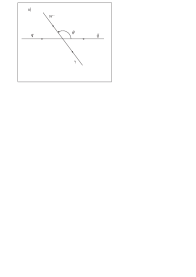
Figure 1: a) The $q\bar{q}^{\prime}\to W\gamma$ collision process and b) the zero in the angular distribution for $W\gamma$ production.

The position of the zero depends only on the charge of the quark (no helicity dependence) :

$$\cos\theta=-(1+2Q_{i}),$$ (1)

where $\theta$ is the angle between $W^{-}$ and $d$ quark (see Fig. 1a), and $Q_{i}$ is the electric charge of the quark in units of the proton charge $e$.

The value of $\cos\theta=-1/3$ (see Fig. 1b), obtained from Eq. (1), is in fact, characteristic for some other SM based process amplitudes too, as we will discuss later.

From the experimental point of view, the Tevatron collider ($p\bar{p}$) is especially well suited to observe the radiation zero predicted in $W\gamma$ production. Sea quark effects tend to wash out the dip caused by the radiation zero. At Tevatron energies, valence quark effects dominate and this effect is not a problem and the radiation zero leaves a clear signature. This is shown in Fig. 2 where we display the distribution of the difference between the rapidities of the $W$ boson, $Y_{W}$, and the photon, $Y_{\gamma}$. The dip at $Y_{\gamma}-Y_{W}\approx 0.3$ is due to the radiation zero Baur_1 .

Figure 2: Rapidity difference distribution for the $p\bar{p}\to W^{-}\gamma$ process.

The boost invariant quantity $Y_{\gamma}-Y_{W}$ contains the same information as the $\cos\theta$ distribution. The $Y_{\gamma}-Y_{W}$ distribution is very similar to the distribution of the rapidity difference between the photon and the charged lepton originating from the $W$ decay, which can be readily observed. This is due to the $V-A$ nature of the $W$ fermion antifermion coupling and the fact that $W$’s in $W\gamma$ production in the SM are strongly polarized: the dominant helicity of the $W^{\pm}$ boson in SM $W^{\pm}\gamma$ production is $\lambda_{W}=\pm 1$.

III Classical Radiation Zeros

In this section we briefly review the classical radiation zeros, which in fact are the limiting case of the so called TYPE I zeros in quantum field theory, which will be discussed in the next section Brown_1 .

It is well known that the electromagnetic radiation originating from a dipole with dipole moment

$$\vec{d}=\sum_{i}Q_{i}\vec{r}_{i}$$ (2)

vanishes, if

$$Q_{i}/m_{i}=Q_{1}/m_{1},~{}{\rm for~{}all}~{}i.$$ (3)

For particles with spin, the magnetic dipole moment is:

$$\vec{\mu}=\sum_{i}\vec{\mu}_{i}=\sum_{i}g_{i}\,\frac{Q_{i}}{2m_{i}}\,\vec{S}_{i}.$$ (4)

If the constants $g_{i}$ are the same for all particles, the condition of Eq. (3) is satisfied, and there are no external torques,

$$\stackrel{{\scriptstyle\cdot}}{{\vec{\mu}}}=0$$ (5)

no radiation occurs.

For the scattering of $relativistic$ particles, the amplitude for photon radiation in the infrared limit can be written in the form

$$A_{IR}=\sum_{i}\frac{Q_{i}}{p_{i}\cdot q}\,\delta_{i}p_{i}\cdot\epsilon$$ (6)

where $\delta_{i}p_{i}=p_{i}~{}(-p_{i})$ before (after) photon radiation. If

$$\frac{Q_{i}}{p_{i}\cdot q}={\rm const,~{}~{}for~{}all}~{}i$$ (7)

where $q$ is the momentum of the photon, then $A_{IR}=0$ from momentum conservation and the transversality condition $q\cdot\epsilon=0$. From Eq. (7) we observe that the condition for a radiation zero in the case of the scattering of relativistic particles via the dot product in the denominator exhibits a dependence on the scattering angle of the photon.

IV Radiation Zeros in Quantum Field Theory

The amplitude zero observed in $W\gamma$ production belongs to the family of so-called “TYPE I” zeros which can be explained as a consequence of the factorization of the amplitude, shown soon after they were first discussed in the literature Brown_1 -Goebel .

The scattering amplitude for the above mentioned process can be obtained starting from the vertices which describe the interaction of the charged particles, attach a photon to each charged particle leg in turn and add all diagrams, as schematically depicted below:

One can show that the amplitude (for particles of any spin) can be written in the form

$$M_{\gamma}=\sum_{i}\frac{A_{i}B_{i}}{C_{i}}$$ (8)

where $A_{i}$ and $B_{i}$ are factors which depend on the charge and polarization. $C_{i}$ represent the particle propagators. This leads to the factorization of the amplitude into separately charge dependent and polarization dependent factors:

$$\sum_{i}\frac{A_{i}B_{i}}{C_{i}}=f(A_{i},C_{i})\cdot g(B_{i},C_{i})$$ (9)

The factorization of the amplitudes holds for any gauge theory based vertex with no restriction on the number of particles, due to the relation between the photon (gauge boson) coupling and Poincare invariance. For the complete tree level amplitude for a source graph $V_{G}$ consisting of a single vertex (no internal lines)

$$M_{\gamma}(V_{G})=\sum\frac{Q_{i}J_{i}}{p_{i}\cdot q}$$ (10)

the vertex currents $J_{i}$ which depend on the polarizations, but not on the charges of the particles obey the identity

$$\sum J_{i}=0$$ (11)

for all Yang-Mills type vertices, as a result of momentum conservation, Lorentz invariance and the Bianchi identity. Thus the vertex amplitude $M_{\gamma}(V_{G})$ vanishes if

$$\frac{Q_{i}}{p_{i}\cdot q}={\rm const,~{}for~{}all}~{}i$$ (12)

similar to the classical case (charge null zone). The well-known radiation zero occurring in $W\gamma$ production belongs to this type.

Since $\sum Q_{i}=0$, the amplitude $M_{\gamma}(V_{G})$ will be zero, if

$$\frac{J_{i}}{p_{i}\cdot q}={\rm const,~{}for~{}all}~{}i$$ (13)

or

$$\frac{p_{i}\cdot\epsilon}{p_{i}\cdot q}={\rm const,~{}for~{}all}~{}i$$ (14)

These zeros correspond to the current null zone Brown_2 .

From the conditions above we see that the null zones connect intrinsic (charge, spin) and space-time properties (Poincare transformation) of the particles involved. This makes it possible to use them in analyzing the structure of the SM.

Radiation zeros can also be explained as a consequence of the decoupling theorem Brown_3 . The wave function of a system of particles in an external Yang-Mills field can be written as

$$\Psi(x)=ULT\chi(x)$$ (15)

where $\chi(x)$ is the free solution of the field equations ($Q=0$, no gauge boson emission), and $ULT$ is the product of the local gauge ($U$), Lorentz ($L$), and displacement ($T$) transformations. The null zone condition

$$\prod_{i}(ULT)_{i}=1$$ (16)

leads to the charge null condition discussed above.

From the condition for the charge null zone we conclude that (since $p_{i}\cdot q\geq 0$)

$$\frac{Q_{i}}{Q_{j}}\geq 0,~{}{\rm for~{}all}~{}i,j.$$ (17)

Notice that the zeros will not necessarily be in the physical range of the parameters ($-1\leq\cos\theta\leq 1$ in the case discussed here).

In $2\to 2$ scattering processes, where one of the final particles is a massless, neutral gauge boson, in the relativistic limit, the zeros occur at the angle

$$\cos\theta=\frac{Q_{1}-Q_{2}}{Q_{2}+Q_{1}},$$ (18)

where $Q_{1}$ and $Q_{2}$ are the charges of the initial state particles.

For the reaction $d\bar{u}\to W^{-}\gamma$ we indeed get $\cos\theta=-\frac{1}{3}$, consistent with the result from a direct computation of the matrix elements. The presence of amplitude zeros also requires a gyro-magnetic factor of $g=2$. Any anomalous $WW\gamma$ coupling changes the value of $g$ and destroys the radiation zero.

V Examples of TYPE I and TYPE II Zeros

Amplitude zeros can be observed in many interesting reactions. In this section we discuss several examples.

A radiation zero exists not only when one massless neutral gauge boson is emitted, but also if two or more are radiated, provided that the neutral gauge bosons are all collinear Brown_4 -Baur_2 . The radiation zero is located at the same scattering angle as in the case where only one boson is radiated. This is illustrated in Fig. 3a where we show the squared amplitude as a function of the photon scattering angle for $W\gamma\gamma$ production at $\sqrt{\hat{s}}=300$ GeV. A $p_{T}(\gamma)>5$ GeV cut has been imposed to avoid the infrared singularities associated with photon emission.

In the case of massive neutral gauge bosons, the radiation zero will have an approximate character. Only some of the amplitudes will exhibit a true zero, which is weakly energy dependent. Fig. 3b shows the $d\bar{u}\to W^{-}Z$ squared helicity amplitude for $\lambda_{W}=-1$ and $\lambda_{Z}=+1$ where $\lambda_{W}$ ($\lambda_{Z}$) is the helicity of the $W$ ($Z$) boson Baur_3 .

Figure 3: Zeros in a) $W\gamma\gamma$, and b) $WZ$ production.

Recently another type of the zeros (TYPE II) was discovered Heyssler_1 -Stirling in the physical phase space range for the processes

$$e^{+}u\to e^{+}u+\gamma,\qquad e^{+}d\to e^{+}d+\gamma,$$ (19)

and

$$q\bar{q}\to W^{+}W^{-}\gamma$$ (20)

Type II zeros occur only if the emitted photons are located in the scattering plane.

VI Zeros in $WZ$, $WZ\gamma$ and $WZZ$ production

In addition to the approximate radiation zero in $q\bar{q}\to W^{\pm}Z$, some of the helicity amplitudes in this process show additional spin-dependent zeros in the physical region. Some of these are approximately symmetric in $\cos\theta$. As an example we show the $d\bar{u}\to W^{-}Z$ squared amplitude for $(\lambda_{W},\lambda_{Z})=(1,1)$ and in Fig. 4a. The $Y_{Z}-Y_{W}$ rapidity difference distribution at the LHC for this helicity combination is shown in Fig. 4b. Unfortunately the amplitudes for which these zeros occur contribute negligibly to the cross section so that it will be very difficult to observe the dips shown in Fig. 4b.

Figure 4: a) The squared $(\lambda_{W},\lambda_{Z})=(1,1)$ amplitude as a function of the scattering angle and b) the $Y_{Z}-Y_{W}$ distribution for $(\lambda_{W},\lambda_{Z})=(1,1)$ in $W^{-}Z$ production at the LHC.

Figure 5: Zeros in $d\bar{u}\to WZ$ and $d\bar{u}\to WZ\gamma$ for a center of mass energy of $E_{c.m.}=173$ GeV. Shown are the squared amplitudes for $(\lambda_{W},\lambda_{Z})=(0,-1)$ and $(\lambda_{W},\lambda_{Z},\lambda_{\gamma})=(0,-1,-1)$. A $p_{T}(\gamma)>0.05$ GeV cut has been imposed to avoid the infrared singularity present in $WZ\gamma$ production. In the $WZ\gamma$ case, the $Z$ boson and the photon are collinear.

The amplitude zeros in the $q\bar{q}\to WZ\gamma,~{}WZZ$ processes are especially interesting, as they originate from different sources. An example given in Fig. 5 shows that the $WZ\gamma$ production amplitude has an additional zero at $\cos\theta=-1/3$ besides the zeros present in $WZ$ production.

In Fig. 5 we have evaluated the matrix element near the threshold, $\sqrt{\hat{s}}\approx M_{W}+M_{Z}$. At threshold, the $W^{-}Z\gamma$ amplitude factorizes into the $W^{-}Z$ amplitude and a factor describing photon emission. This factor exhibits an energy independent zero at $\cos\theta_{\gamma}=1/3$ if the $Z$ boson and photon are collinear. Here, $\theta_{\gamma}$ is the angle between the incoming $d$ quark and the photon. The other zeros originate from the $WZ$ production amplitude.

To summarize, the $WZ\gamma$ production amplitudes have a very rich structure with zeros originating from three different sources:
1. a radiation zero at $\cos\theta_{\gamma}=1/3$ connected with photon radiation
2. the approximate radiation zero occurring in $WZ$ production,
3. the spin dependent zeros in some of the $WZ$ production amplitudes discussed above.
The zero present at $\cos\theta_{\gamma}=1/3$ leads to a clear dip in the $Y_{Z\gamma}-Y_{W}$ rapidity difference distribution ($Y_{Z\gamma}$ is the rapidity of the $Z\gamma$ system) if the cosine of the angle between the $Z$ boson and photon is restricted to $\cos\theta(Z,\gamma)>0$. The $Y_{Z\gamma}-Y_{W}$ distribution at the LHC is shown in Fig. 6.

Figure 6: The $Y_{Z\gamma}-Y_{W}$ rapidity difference distribution for $\cos\theta(Z,\gamma)>0$ in $W^{-}Z\gamma$ production at the LHC.

Figure 7: Comparison of the $Y_{Z\gamma}-Y_{W}$ distribution in $WZ\gamma$ production, and the $Y_{ZZ}-Y_{W}$ distribution in $WZZ$ production at the LHC.

Similar to $WZ$ production, the amplitudes for $WZZ$ production exhibit an approximate radiation zero if the two $Z$ bosons are collinear. It leads to a dip in the $Y_{ZZ}-Y_{W}$ distribution, which, however, is much less pronounced than the corresponding dip in the $Y_{Z\gamma}-Y_{W}$ distribution in $WZ\gamma$ production. A comparison of the two distributions at the LHC is shown in Fig. 7. Only the helicity amplitudes which give the dominating contributions to the cross section have been taken into account here.

The radiation zeros can be used for testing the models beyond the SM Baur_4 -Gangemi . Any anomalous coupling term added to the Lagrangian causes the dips originating from the amplitude zeros to be washed out. In Fig. 8 we show how an anomalous coupling described by the effective Lagrangian

$$L~{}=~{}\frac{g_{c}g^{2}}{cos^{2}\theta_{W}}W_{\mu}Z^{\mu}W_{\nu}Z^{\nu}$$ (21)

with $g_{c}=0.05$ affects the $Y_{ZZ}-Y_{W}$ distribution in $WZZ$ production Belanger .

Figure 8: The $Y_{ZZ}-Y_{W}$ distribution in $WZZ$ production at the LHC. The solid histogram shows the SM prediction. The dashed histogram shows the $Y_{ZZ}-Y_{W}$ distribution for $g_{c}=0.05$.

VII CONCLUSION

Radiation zeros are a consequence of the factorization of tree level amplitudes in the SM. The zeros occur for processes where one or more neutral, massless gauge bosons are radiated. If the emitted gauge boson is massive, only some of the helicity amplitudes exhibit zeros. Radiation zeros leave deep measurable dips in rapidity difference distributions for many hadron collider processes, such as $W\gamma$, $WZ$, $WZZ$ and $WZ\gamma$ production. Since anomalous coupling terms destroy the radiation zeros, they can be used for probing the SM.

References

- (1) Lee, T.D., Yang, C.N., Phys. Rev. 128, 885-898 (1962).
- (2) Mikaelyan, K.O., Samuel M.A., and Sahdev, D., Phys. Rev. Lett. 43, 746-749 (1979).
- (3) Baur, U., Errede, S. and Landsberg, G. , Phys. Rev. D50, 1917-1930 (1983).
- (4) Brown, R.W., Kowalski, K.L., and S. J. Brodsky, Phys. Rev. D28, 624-649 (1983).
- (5) Dongpei, Zhu, Phys. Rev. D22, 2266-2274 (1980).
- (6) Goebel, C.J., Halzen, F., and Leveille, J.P., Phys. Rev. D23, 2682-2685 (1980).
- (7) Brown, R.W., and Kowalski, K.L., Phys. Rev. D29, 2100-2104 (1984).
- (8) Brown, R.W., and Kowalski, K.L., Phys. Rev. Lett. 51, 2355-2358 (1983).
- (9) Brown, R.W., Convery, M.E., and Samuel, M. A., Phys. Rev. D49, 2290-2297 (1994).
- (10) Brown, R.W., Vector Boson Symp. 1995, 261-272, hep-ph/9506018.
- (11) Baur, U., Han, T., Kauer, N., Sobey, R., and Zeppenfeld, D., Phys. Rev. D56, 140-150 (1997).
- (12) Baur, U., Han, T., and Ohnemus, J., Phys. Rev. Lett. 72, 3941-3944 (1994).
- (13) Heyssler M., and Stirling, W.J., Eur. Phys. J. C4, 289-299 (1998).
- (14) Heyssler M., and Stirling, W.J., Eur. Phys. J. C5, 475-484 (1998).
- (15) Stirling, W. James, and Werthenbach, Anna, Eur. Phys. J. C12, 441-450 (2000).
- (16) Baur, U., Zeppenfeld, D., Phys. Lett. B201, 383-389 (1988).
- (17) Belanger, G., Boudjema, F., Kurihara, Y., Perret-Gallix, D., Semenov, A., Eur.Phys.J. C13, 283-293 (2000).
- (18) Gangemi, F., hep-ph/0002142.