Abstract

We perform a complete analysis of the supersymmetric particle spectrum in the Minimal Supergravity (mSUGRA) model where the soft SUSY breaking scalar masses, gaugino masses and trilinear couplings are unified at the GUT scale, so that the electroweak symmetry is broken radiatively. We show that the present constraints on the Higgs boson and superparticle masses from collider searches and precision measurements still allow for large regions of the mSUGRA parameter space where charginos, neutralinos, sleptons and top squarks as well as the heavier Higgs particles, are light enough to be produced at the next generation of $e^{+}e^{-}$ linear colliders with center of mass energy around $\sqrt{s}\sim 800$ GeV, with sizeable cross sections. An important part of this parameter space remains even when we require that the density of the lightest neutralinos left over from the Big Bang, which we calculate using standard assumptions, falls in the range favored by current determinations of the Dark Matter density in the Universe. Already at a c.m. energy of 500 GeV, SUSY particles can be accessible in some parameter range, and if the energy is increased to $\sqrt{s}\simeq 1.2$ TeV, the $e^{+}e^{-}$ collider will have a reach for high precision studies of SUSY particles in a range that is comparable to the discovery range of the LHC.

1. Introduction

Supersymmetric theories (SUSY) [1] are the best motivated extensions of the Standard Model (SM) of the electroweak and strong interactions. They provide an elegant way to stabilize the huge hierarchy between the Grand Unification (GUT) or Planck scale and the Fermi scale, providing a natural framework to cancel the quadratic divergences of the radiative corrections to the Higgs boson mass. The most economical low–energy supersymmetric extension of the SM, the Minimal Supersymmetric Standard Model (MSSM) [2], allows for a consistent unification of the three coupling constants of the SM gauge group [3]. In addition, it can provide a natural solution of the Dark Matter problem [4], since it predicts the existence of an electrically neutral, weakly interacting, massive and absolutely stable particle; for large regions of parameter space the thermal relic density of this particle agrees with the Dark Matter density derived from cosmological arguments. The search for Supersymmetric particles and for the required extended Higgs spectrum is one of the main motivations for building high–energy colliders.

In the MSSM one assumes the minimal gauge group, i.e. the SM ${\rm SU(3)_{C}\times SU(2)_{L}\times U(1)_{Y}}$ group; the minimal particle content, i.e. three generations of fermions [without right–handed neutrinos] and their spin–zero partners as well as two Higgs doublet superfields to break the electroweak symmetry; and R–parity conservation [5] which makes the lightest SUSY particle, assumed to be the lightest neutralino $\tilde{\chi}_{1}^{0}$, absolutely stable. In order to explicitly break supersymmetry [as required by experiment] while preventing the reappearance of quadratic divergences, a collection of soft terms is added to the Lagrangian [6]: mass terms for the gauginos, mass terms for the scalar fermions, mass and bilinear terms for the Higgs bosons, and trilinear couplings between sfermions and Higgs bosons. In the general case, that is if one allows for intergenerational mixing and complex phases, the soft SUSY breaking terms will introduce a huge number (105) of unknown parameters [7], in addition to the 19 parameters of the SM.

This feature makes any phenomenological analysis in the general MSSM a daunting task, if possible at all. In addition, almost all “generic” sets of these parameters are excluded by severe phenomenological constraints, on flavor changing neutral currents (FCNC), additional CP–violation, color and charge breaking minima, etc. Almost all FCNC problems are solved at once if the MSSM parameters obey a set of universal boundary conditions at the GUT scale. We will take these parameters to be real, which solves all problems with CP violation. The underlying assumption is that SUSY–breaking occurs in a hidden sector which communicates with the visible sector only through gravitational–strength interactions, as specified by supergravity [10]. Universal soft breaking terms then emerge if these supergravity interactions are “flavor–blind” [like ordinary gravitational interactions]. This is assumed to be the case in the constrained MSSM or minimal Supergravity (mSUGRA) model [11]. In this model the entire spectrum of superparticles and Higgs bosons is determined by the values of five free parameters. Since universal boundary conditions imply that the electroweak symmetry is broken radiatively, which imposes one constraint on the input parameters, one is left with only four continuous free parameters and a discrete one. This makes comprehensive scans of parameter space feasible.

Although other viable SUSY models exist, the mSUGRA model has become the most frequently used benchmark scenario for supersymmetry, and has been widely used to analyze the expected SUSY particle spectrum and the properties of SUSY particles, and to compare the predictions with available and/or expected data from collider experiments. Several global or partial analyses of the present theoretical and experimental constraints on the mSUGRA model have been performed in the literature; see for instance Refs. [12, 13, 14].

In this paper, we perform an independent analysis of the SUSY particle spectrum in the mSUGRA model, taking into account theoretical constraints and all available experimental information [15]: searches for the MSSM Higgs bosons and SUSY particles at the LEP and Tevatron colliders, electroweak precision measurements, the radiative $b\to s\gamma$ decay, etc. Special attention is paid to the implications of the measurement of the anomalous magnetic moment of the muon recently performed at Brookhaven [16], and to the $\sim 2\sigma$ evidence for a SM–like Higgs boson with a mass $M_{\rm Higgs}\sim 115.6$ GeV seen by the LEP collaborations [17]. We also discuss the implication of requiring thermal relic neutralinos to form the Dark Matter in the Universe.

We show that in a large part of the mSUGRA parameter space at least one of these independent pieces of evidence for physics beyond the SM, from the Dark Matter density, the $(g_{\mu}-2)$ measurement and the LEP2 Higgs boson–like excess, can be explained in mSUGRA. On the other hand, only a small area of parameter space allows for these three constraints to be fulfilled simultaneously. If all these indications survive further scrutiny, the parameter space of the model would thus already be tightly constrained. However, one has to keep in mind that the statistical significance for the LEP Higgs signal and the $(g_{\mu}-2)$ anomaly are at present still quite weak, while the calculation of the thermal relic density relies on additional assumptions that cannot be tested in collider experiments.

We then discuss prospects for producing SUSY particles and the heavier Higgs bosons of the MSSM at future high–energy $e^{+}e^{-}$ linear colliders with center of mass energies $\sqrt{s}$ around 800 GeV as expected, for instance, at the TESLA machine [24]. We show that in large areas of the mSUGRA parameter space the production rates for the lightest charginos and neutralinos, as well as for sleptons, top squarks and the heavier Higgs bosons are large enough for these particles to be discovered, given the very large integrated luminosities, ${\cal L}\sim 500$ fb^-1, expected at this collider. Even at lower energies, $\sqrt{s}\simeq 500$ GeV, charginos, neutralinos and tau sleptons can be produced in some parameter range. If the energy is raised to $\sqrt{s}\simeq 1.2$ TeV [25], the $e^{+}e^{-}$ collider will have a reach for probing the SUSY particle spectrum and the heavy Higgs bosons which is comparable to the reach of the LHC.

The remainder of this paper is organized as follows. In the next section we briefly summarize the main features of the mSUGRA model and the way it is implemented in our analysis. In section 3 the experimental and cosmological constraints on the mSUGRA parameter space are discussed. In section 4 we analyze the production of SUSY particles and MSSM Higgs bosons at high energy $e^{+}e^{-}$ colliders. Conclusions are given in section 5. For completeness, expressions for the cross sections of all discussed particle production channels in $e^{+}e^{-}$ collisions are collected in the Appendix.

2. The Physical Set–Up

2.1 The mSUGRA model

We will perform our analysis in the constrained MSSM or minimal Supergravity model, where the MSSM soft breaking parameters obey a set of universal boundary conditions at the GUT scale, so that the electroweak symmetry is broken radiatively. For completeness and to fix the notation, let us list these unification and universality hypotheses and summarize the main features of the radiative electroweak symmetry breaking (EWSB) mechanism.

Besides the unification of the gauge coupling constants, which is verified given the experimental results from LEP1 [3] and which can be viewed as fixing the Grand Unification scale $M_{\rm GUT}\sim 2\cdot 10^{16}$ GeV, the unification conditions are as follows:

– Unification of the gaugino [bino, wino and gluino] masses:

$$M_{1}(M_{\rm GUT})=M_{2}(M_{\rm GUT})=M_{3}(M_{\rm GUT})\equiv m_{1/2}.$$ (1)

– Universal scalar [sfermion and Higgs boson] masses [$i$ is a generation index]

$$M_{\tilde{Q}^{i}}(M_{\rm GUT}) = M_{\tilde{u}^{i}_{R}}(M_{\rm GUT})=M_{\tilde{d}^{i}_{R}}(M_{\rm GUT})=M_{\tilde{L}^{i}}(M_{\rm GUT})=M_{\tilde{l}^{i}_{R}}(M_{\rm GUT})$$ (2)

$$= M_{H_{u}}(M_{\rm GUT})=M_{H_{d}}(M_{\rm GUT})\equiv m_{0}.$$

– Universal trilinear couplings:

$$A_{u}^{ij}(M_{\rm GUT})=A_{d}^{ij}(M_{\rm GUT})=A_{l}^{ij}(M_{\rm GUT})\equiv A_{0}\delta_{ij}.$$ (3)

Besides the three parameters $m_{1/2},m_{0}$ and $A_{0}$, the supersymmetric sector is described at the GUT scale by the bilinear coupling $B$ and the supersymmetric Higgs(ino) mass parameter $\mu$. However, one has to require that EWSB takes place. This results in two necessary minimization conditions of the two Higgs doublet scalar potential which, at the tree–level, has the form [26] [to have a more precise description, one–loop corrections to the scalar potential have to be included, as will be discussed later]:

$$V_{\rm Higgs} = \overline{m}_{1}^{2}H_{d}^{\dagger}H_{d}+\overline{m}_{2}^{2}H_{u}^{\dagger}H_{u}+\overline{m}_{3}^{2}(H_{u}\cdot H_{d}+{\rm h.c.})$$ (4)

$$+ \frac{g_{1}^{2}+g_{2}^{2}}{8}(H_{d}^{\dagger}H_{d}-H_{u}^{\dagger}H_{u})^{2}+\frac{g_{2}^{2}}{2}(H_{d}^{\dagger}H_{u})(H_{u}^{\dagger}H_{d}),$$

where we have used the usual short–hand notation:

$$\overline{m}_{1}^{2}=m^{2}_{H_{d}}+\mu^{2}\ ,\ \overline{m}_{2}^{2}=m^{2}_{H_{u}}+\mu^{2}\ ,\ \overline{m}_{3}^{2}=B\mu.$$ (5)

The SU(2) invariant product of two doublets is defined as $\phi_{1}\cdot\phi_{2}=\phi_{1}^{1}\phi_{2}^{2}-\phi_{1}^{2}\phi_{2}^{1}$, where the superscripts are SU(2) indices. The two minimization equations $\partial V_{\rm Higgs}/\partial H_{d}^{0}=\partial V_{\rm Higgs}/\partial H_{u}^{0}=0$ can be solved for $\mu^{2}$ and $B\mu$:

$$\mu^{2} = \frac{1}{2}\bigg{[}\tan 2\beta(m^{2}_{H_{u}}\tan\beta-m^{2}_{H_{d}}\cot\beta)-M_{Z}^{2}\bigg{]};$$

$$B\mu = \frac{1}{2}\sin 2\beta\Bigg{[}m^{2}_{H_{u}}+m^{2}_{H_{d}}+2\mu^{2}\Bigg{]}.$$ (6)

Here, $M_{Z}^{2}=(g_{1}^{2}+g_{2}^{2})\cdot(v_{u}^{2}+v_{d}^{2})/4$, and $\tan\beta=v_{u}/v_{d}$ is defined in terms of the vacuum expectation values of the two neutral Higgs fields. Consistent EWSB is only possible if eq. (2.1 The mSUGRA model) gives a positive value of $\mu^{2}$. The sign of $\mu$ is not determined. Therefore, in this model one is left with only four continuous free parameters, and an unknown sign:

$$\tan\beta\ ,\ m_{1/2}\ ,\ m_{0}\ ,\ A_{0}\ ,\ \ {\rm sign}(\mu).$$ (7)

All the soft SUSY breaking parameters at the weak scale are then obtained through Renormalization Group Equations (RGE) [27].

The number of parameters could be further reduced by introducing an additional constraint which is based on the assumption that the $b$ and $\tau$ Yukawa couplings unify at the GUT scale, as predicted in minimal SU(5). This restricts $\tan\beta$ to two narrow ranges around $\tan\beta\sim 1.5$ and $\tan\beta\sim m_{t}/m_{b}$ [28]. The low $\tan\beta$ solution is ruled out since it leads to a too light an $h$ boson, in conflict with searches at LEP2. However, Yukawa unification is not particularly natural in the context of superstring theories, and minimal SU(5) predictions are known to fail badly for the lighter generations. We therefore treat all three third generation Yukawa couplings as independent free parameters.

2.2 Calculation of the SUSY particle spectrum

In this section, we briefly discuss our procedure for calculating the SUSY particle spectrum in the constrained MSSM with universal boundary conditions at the GUT scale, as well as related issues which are relevant to our study. All results are based on the numerical FORTRAN code SuSpect version 2.0 [29], to which we refer for a more detailed description. The algorithm essentially includes:

• Renormalization group evolution (RGE) of parameters between the low energy scale [$M_{Z}$ and/or the electroweak symmetry breaking scale] and the GUT scale.

• Consistent implementation of radiative electroweak symmetry breaking (EWSB). Loop corrections to the effective potential are included using the tadpole method.

• Calculation of the physical (pole) masses of the Higgs bosons, scalar quarks and leptons as well as gluinos, charginos and neutralinos.

In more detail we proceed as follows. We first chose the low–energy input values of the SM parameters. The gauge couplings constants are defined in the ${\overline{\rm MS}}$ scheme at the scale $M_{Z}$ [$\bar{s}_{W}^{2}=1-\bar{c}_{W}^{2}\equiv\sin^{2}\theta_{W}|^{\overline{\rm MS}}$]:

$$g_{1}^{2}=\frac{4\pi\alpha^{\overline{\rm MS}}_{\rm em}(M_{Z})}{\bar{c}^{2}_{W}}\ ,\ g_{2}^{2}=\frac{4\pi\alpha^{\overline{\rm MS}}_{\rm em}(M_{Z})}{\bar{s}^{2}_{W}}\ ,\ g_{3}^{2}=4\pi\alpha^{\overline{\rm MS}}_{s}(M_{Z}).$$ (8)

Their values have been obtained from precision measurements at LEP and Tevatron [15]:

$$\alpha^{\overline{\rm MS}}_{\rm em}(M_{Z})=1/127.938\ ,\ \alpha^{\overline{\rm MS}}_{s}(M_{Z})=0.1192\ ,\ \bar{s}^{2}_{W}=0.23117.$$ (9)

The pole masses of the heavy SM fermions are [15]:

$$M_{t}=174.3\ {\rm GeV}\ \ ,\ \ M_{b}=4.62\ {\rm GeV}\ \ ,\ \ M_{\tau}=1.778\ {\rm GeV}\ \ .$$ (10)

From the pole $b$–quark mass, one then obtains the $\overline{\rm DR}$ mass, $\overline{m}_{b}(\overline{m}_{b})\simeq 4.23$ GeV which is then evolved, using two–loop ${\cal O}(\alpha_{s}^{2})$ RGE, to obtain the running mass at the scale $M_{Z}$, $\overline{m}_{b}(M_{Z})\simeq 2.92$ GeV. Since the two–loop corrections to the difference between pole and $\overline{\rm DR}$ top and bottom quark masses are not yet known, we include, instead, the analogous two–loop corrections in the $\overline{\rm MS}$ scheme, which should be close to the $\overline{\rm DR}$ ones. The difference should not be important in view of the experimental errors in the determination of the two masses [15], $M_{t}=174.3\pm 5.1$ GeV and $\overline{m}_{b}(\overline{m}_{b})\simeq 4.24\pm 0.11$ GeV.

Next, the $\overline{\rm DR}$–scheme values of the gauge and Yukawa couplings are extracted from these inputs [30]. The latter are defined by [$v=174.1$ GeV]:

$$\lambda_{t}(M_{t})=\frac{\overline{m}_{t}(M_{t})}{v\sin\beta}\ ,\ \lambda_{b}(M_{Z})=\frac{\overline{m}_{b}(M_{Z})}{v\cos\beta}\ ,\ \lambda_{\tau}(M_{Z})=\frac{\overline{m}_{\tau}(M_{Z})}{v\cos\beta}\ .$$ (11)

All couplings are then evolved up to the GUT scale using two–loop RGEs [30, 31]. Here heavy (super)particles are taken to contribute to the RGE only at scales larger than their mass, i.e. multiple thresholds are included in the running of the coupling constants near the weak scale. The GUT scale $M_{\rm GUT}\simeq 2\cdot 10^{16}$ GeV is defined to be the scale at which $g_{1}=g_{2}\cdot\sqrt{3/5}$. We do not enforce $g_{2}=g_{3}$ at the GUT scale and assume that the small discrepancy [of the order of a few percent] is accounted for by unknown GUT–scale threshold corrections [32].

In our numerical analyses we fix the MSSM parameters $\tan\beta$ [given at scale $M_{Z}$] as well as $A_{0}$ and the sign of $\mu$, and then perform a systematic scan over the high energy mSUGRA inputs $m_{0}$ and $m_{1/2}$. Given these boundary conditions, all the soft SUSY breaking parameters and couplings are evolved down to the electroweak scale. Our default choice for this scale is the geometric mean of the two top squark masses, $M_{\rm EWSB}=(m_{\tilde{t}_{1}}m_{\tilde{t}_{2}})^{1/2}$, which minimizes the scale-dependence of the one–loop scalar effective potential [33]. Since $\tan\beta$ is defined at scale $M_{Z}$, the vevs have to be evolved down from $M_{\rm EWSB}$ to $M_{Z}$ [33].

One–loop radiative corrections to the Higgs potential play a major role in determining the values of the parameters $|\mu|$ and $B$ in terms of the soft SUSY breaking masses of the two Higgs doublet fields. We treat these corrections using the tadpole method. This means that we can still use eq. (2.1 The mSUGRA model) to determine $\mu^{2}(M_{\rm EWSB})$; one simply has to add one–loop tadpole corrections to $m^{2}_{H_{d}}$ and $m^{2}_{H_{u}}$ [34, 35]. We include the dominant third generation fermion and sfermion loops, as well as subdominant contributions from sfermions of the first two generations, gauge bosons, Higgs bosons, charginos and neutralinos, with the running parameters evaluated at $M_{\rm EWSB}$. As far as the determination of $\mu^{2}$ and $B\mu$ is concerned, this is equivalent to computing the full one–loop effective potential at scale $M_{\rm EWSB}$. Since $|\mu|$ and $B$ affect masses of some (s)particles appearing in these corrections, this procedure has to be iterated until stability is reached and a consistent value of $\mu$ is obtained; usually this requires only three or four iterations for an accuracy of ${\cal O}(10^{-4})$, if one starts from the values of $|\mu|$ and $B$ as determined from minimization of the RG–improved tree–level potential at scale $M_{\rm EWSB}$.

At this stage, we check whether the complete scalar potential has charge and/or color breaking (CCB) minima, which can be lower than the electroweak minimum. These can e.g. appear in the top squark sector for large values of the trilinear coupling $A_{t}$. In order to avoid them, we impose the (simplest) condition [37]:

$${\rm CCB}: A^{2}_{t}<3\,(m^{2}_{\tilde{t}_{L}}+m^{2}_{\tilde{t}_{R}}+\mu^{2}+m^{2}_{H_{u}}).$$ (12)

Of course, we also reject all points in the parameter space which lead to tachyonic Higgs boson or sfermion masses:

$${\rm No\,Tachyon}: M_{A}^{2}>0\ \ ,M^{2}_{h}>0\ \ ,\ \ m^{2}_{\tilde{f}}>0.$$ (13)

The EWSB mechanism is assumed to be consistent when all these conditions are satisfied.

We then calculate all physical particle masses. The procedure is iterated at least twice until stability is reached, in order to take into account: (i) Realistic (multi–scale) particle thresholds in the RG evolution of the dimensionless couplings via step functions in the $\beta$ functions for each particle threshold. (ii) Radiative corrections to SUSY particle masses, using the expressions given in Ref. [35], where the renormalization scale is set to $M_{\rm EWSB}$.

We first evaluate the SUSY–radiative corrections to the heavy fermion masses, $\bar{m}_{t},\ \bar{m}_{b}$ and $\bar{m}_{\tau}$, following Ref. [35]. This includes SUSY–QCD corrections for the $t,b$ quarks [from squark–gluino loops] and the dominant electroweak corrections for the $b$ and $\tau$ masses [chargino–sfermion loops which are enhanced by terms $\propto\mu\tan\beta$]. As suggested in Ref. [38], we use the “MSSM” quark masses [essentially the Yukawa coupling times vev] in the squark mass matrices. Our iteration then resums all SUSY–QCD corrections to the quark masses of order $\left(\alpha_{s}\tan\beta\right)^{n}$. This is important at large $\tan\beta$, where these corrections can be quite sizable. The various sectors of the MSSM are then treated as follows:

– In the sfermion sector, the soft scalar masses as well as the trilinear couplings for the third generation are obtained using one–loop RGE, and are frozen at the scale $M_{\rm EWSB}$. In the third generation sfermion sector [$\tilde{t},\tilde{b},\tilde{\tau}$], mixing between “left” and “right” current eigenstates is included, where the radiatively corrected running fermion masses at scale $M_{\rm EWSB}$ are employed in the sfermion mass matrices. The radiative corrections to the sfermion masses are included according to Ref. [35], i.e. only the QCD corrections for the superpartners of light quarks [including the bottom squark] plus the leading electroweak corrections to the top squarks; the small electroweak radiative corrections to the slepton masses have been neglected.

– In the gaugino sector, the SUSY breaking gaugino masses are obtained using the two–loop RGEs and are also frozen at $M_{\rm EWSB}$. The mass matrices for charginos and neutralinos are diagonalized using analytical formulae [39]. The one–loop QCD radiative corrections to the gluino mass are incorporated [30], while in the case of charginos and neutralinos the radiative corrections [40] are included in the gaugino and higgsino limits, which is a very good approximation according to Ref. [35].

– In the Higgs sector, the running mass of the pseudoscalar Higgs boson is obtained from the soft SUSY breaking Higgs masses [again frozen at $M_{\rm EWSB}$] and the full one–loop tadpole corrections [35]. This mass is then used as input, together with $M_{t},\ \tan\beta$ and some MSSM parameters [$A_{t},A_{b},\mu$ and the soft SUSY breaking third generation squark masses], to obtain the pole masses of the pseudoscalar Higgs boson $A$, the two CP–even $h$ and $H$ bosons and the charged $H^{\pm}$ Higgs particles. This last step is similar to the program HDECAY [41], which calculates the Higgs spectrum and decay widths in the MSSM. The complete radiative corrections due to top/bottom quark and squark loops within the effective potential approach, leading NLO QCD corrections [through renormalization group improvement] and the full mixing in the stop and sbottom sectors are incorporated using the analytical expressions of Ref. [42]. We have verified that the results obtained for the Higgs spectrum, in particular for the lightest $h$ boson mass, are nearly the same as those obtained from the complete results of the Feynman diagrammatic approach implemented in the program FeynHiggs [43].

Our results for some representative points of the mSUGRA parameter space have been carefully cross–checked against other existing codes. We obtain very good agreement, at the one percent level, with the program SOFTSUSY [44] which has been released recently. We also find rather good agreement for the SUSY particle masses computed by the program ISASUGRA [45], once we chose the same configuration [soft SUSY breaking masses frozen at $M_{Z}$, some radiative corrections to sparticle masses are not included, etc..]. The value of the lightest Higgs boson mass is in less good agreement, presumably due to the more sophisticated treatment of the Higgs potential in SuSpect; we will see later that a precise calculation of the $h$ boson mass is an important ingredient of our analysis.

3. Constraints on the mSUGRA parameter space

3.1 Experimental Constraints

i) Lower bounds on the SUSY particles masses

A wide range of searches for SUSY particles has been performed at LEP2 and at the Tevatron, resulting in limits on the masses of these particles [15]. The pair production of the lightest chargino at LEP2, $e^{+}e^{-}\to\tilde{\chi}_{1}^{+}\tilde{\chi}_{1}^{-}$, would probably have been the cleanest SUSY process. In general it has the largest SUSY production cross section at $e^{+}e^{-}$ colliders, after the experimental cuts needed to suppress the backgrounds, and the information that it provides is one of the most important in the context of the mSUGRA model. The negative outcome of searches for charginos at LEP2, up to energies of $\sqrt{s}\simeq 208$ GeV, gives the approximate bound $m_{\tilde{\chi}_{1}^{\pm}}\raisebox{-3.69899pt}{~{}\shortstack{$>$ \\ [-0.07cm] $\sim$}}~{}104$ GeV [46].

In mSUGRA the gaugino masses are unified at the GUT scale, leading to the approximate relation $M_{2}\simeq 2M_{1}\sim M_{3}/3$ at the weak scale. The bound on the lightest chargino mass thus translates into a lower bound on the LSP mass, $m_{\tilde{\chi}_{1}^{0}}\raisebox{-3.69899pt}{~{}\shortstack{$>$ \\ [-0.07cm] $\sim$}}~{}50$ GeV [in the gaugino–like region; in the higgsino–region, the bound is higher] and also on the gluino mass, $m_{\tilde{g}}\sim M_{3}\raisebox{-3.69899pt}{~{}\shortstack{$>$ \\ [-0.07cm] $\sim$}}~{}300$ GeV. In the case of the LSP, the bound can be improved by using searches for neutralino production at LEP2, $e^{+}e^{-}\to\tilde{\chi}_{1}^{0}\tilde{\chi}_{2}^{0}$; however, these neutralino searches are relevant only for low values of $\tan\beta\raisebox{-3.69899pt}{~{}\shortstack{$<$ \\ [-0.07cm] $\sim$}}~{}2$ which are already excluded by Higgs boson searches, as will be discussed later. In the case of gluinos, this indirect bound is similar to the one obtained from direct searches at the Tevatron, $m_{\tilde{g}}\raisebox{-3.69899pt}{~{}\shortstack{$>$ \\ [-0.07cm] $\sim$}}~{}300$ GeV, which is valid if $m_{\tilde{q}}\simeq m_{\tilde{g}}$ [47]; the direct search limits for $m_{\tilde{q}}\gg m_{\tilde{g}}$ are significantly weaker.

The bound on $M_{2}$ also translates into a bound on the masses of first and second generation squarks. The RG evolution of these masses [up to small contribution from the D–terms] gives the approximate relation $m^{2}_{\tilde{q}}\sim m_{0}^{2}+6m_{1/2}^{2}$, which leads to $m_{\tilde{q}}\raisebox{-3.69899pt}{~{}\shortstack{$>$ \\ [-0.07cm] $\sim$}}~{}250$ GeV, again of similar size as the bound from direct searches at the Tevatron [47]. For third generation squarks the RGE are more complicated and mixing between the eigenstates is important, due to the large values of the Yukawa couplings, so that the bounds from direct searches are relevant. We use the bound from LEP2 [46], which is almost independent of the decay modes, and is applicable down to squark$-\mbox{$\tilde{\chi}_{1}^{0}$}$ mass splittings of a few GeV; Tevatron search limits [48] are stronger in some cases, but more dependent on details of squark decay, and disappear for mass splittings below $\sim 30$ GeV.

By far the tightest slepton search limits also come from LEP2 [46]. Here the coefficients of the $m_{1/2}^{2}$ term in the RG evolution of $m^{2}_{\tilde{l}}$ are small so that [at least for the SU(2) singlet “right–handed” states] $m_{\tilde{l}}\sim m_{0}$. These LEP bounds are generally a few GeV below the kinematical limit, except for some small regions of the parameter space with small mass difference to the LSP. Since sneutrinos might decay invisibly into $\nu\tilde{\chi}_{1}^{0}$, only indirect bounds can be placed on their masses. Limits from searches for charged SU(2) doublet sleptons, whose masses are related to sneutrino masses by SU(2), are rather model–independent. In mSUGRA additional indirect limits on sneutrino masses follow from searches for SU(2) singlet sleptons and charginos, via the resulting constraints on $m_{0}$ and $m_{1/2}$.

To summarize, in our analysis we impose the following bounds on sparticle masses:

$$m_{\tilde{\chi}_{1}^{+}}\geq 104~{}{\rm GeV} m_{\tilde{f}}\geq 100\ {\rm GeV\ with}\ \tilde{f}=\tilde{t}_{1},\tilde{b}_{1},\tilde{l}^{\pm},\tilde{\nu}$$ ,

$$m_{\tilde{g}}\geq 300~{}{\rm GeV} m_{\tilde{q}_{1,2}}\geq 260\ {\rm GeV\ with}\ \tilde{q}=\tilde{u},\tilde{d},\tilde{s},\tilde{d}.$$ , (14)

ii) Constraints from the Higgs boson masses

The search for SUSY Higgs bosons was the main motivation for extending the LEP2 energy up to $\sqrt{s}\simeq 208$ GeV. In the SM, a lower bound [49, 17]

$$M_{H^{0}}\ >\ 113.5\ {\rm GeV}\ {\rm at\ the\ 95\%C.L.}$$ (15)

has been set by investigating the Higgs–strahlung process, $e^{+}e^{-}\to ZH^{0}$. In the MSSM, this bound is valid for the lightest CP–even Higgs particle $h$ if its coupling to the $Z$ boson is SM–like, i.e. if $g^{2}_{ZZh}/g^{2}_{ZZH^{0}}\equiv\sin^{2}(\beta-\alpha)\simeq 1$ where $\alpha$ is the mixing angle in the CP–even neutral Higgs sector. This occurs in the decoupling regime where $M_{A}^{2}\gg M_{Z}^{2}$. For much lower values of $M_{A}$ and for large $\tan\beta$, one has $M_{h}\sim M_{A}$ and $\sin^{2}(\beta-\alpha)\ll 1$. In this case, the bound (15) applies to the mass of the heavy neutral CP–even Higgs boson $H$. However, tighter constraints on the parameter space can usually be derived from the search for the associated production of CP–even and CP–odd Higgs particles, $e^{+}e^{-}\to hA$, which has a cross section proportional to $\cos^{2}(\beta-\alpha)$. At LEP2, a combined mass exclusion in the MSSM,

$$M_{h}\,\simeq\,M_{A}\,\raisebox{-3.69899pt}{~{}\shortstack{$>$ \\ [-0.07cm] $\sim$}}~{}\,93.5\ {\rm GeV}$$ (16)

at the 95% Confidence Level, has been set in this case. This limit is lower than that from the Higgs–strahlung process, due to the less distinctive signal and the $\beta^{3}$ suppression near threshold for spin–zero particle pair production.

Deriving a precise bound on $M_{h}$ for arbitrary values of $M_{A}$ [not just for $M_{A}^{2}\gg M_{Z}^{2}$ or $M_{A}\simeq M_{h}$] and hence for all values of $\sin^{2}(\beta-\alpha)$ is rather complicated, since one has to combine results from two different production channels, which have different kinematical behavior, cross sections, backgrounds, etc. In our analysis, we will use an interpolation formula for the excluded value of $M_{h}$:

$$M_{h}>93.5+15x+54.3x^{2}-48.4x^{3}-25.7x^{4}+24.8x^{5}-0.5\,{\rm GeV},$$ (17)

with $x=\sin^{2}(\beta-\alpha)$. This formula fits the exclusion plot in the $[M_{h},\sin^{2}(\beta-\alpha)]$ plane given by the ALEPH collaboration in Ref. [50]. At this point we assume a very small theoretical error of 0.5 GeV in the calculation of $M_{h}$ and $M_{A}$, and have lowered the bounds accordingly; this is the typical difference between our value of $M_{h}$ and the one obtained in the full diagrammatic approach [43]. The total theoretical error on the calculated Higgs boson masses is probably much larger, even if all input parameters were known exactly. The intrinsic uncertainty due to unknown higher–order effects is usually estimated to be about two or three GeV. In addition, the error on the top quark mass leads to an uncertainty of the predicted value of $M_{h}$ of a few GeV. The impact of these uncertainties will be discussed later.

We will also study the implications of the $2.1\sigma$ evidence for a SM–like Higgs boson with a mass $M_{H}=115.6$ GeV seen by the LEP collaborations [17]. In view of the theoretical and experimental uncertainties, we interpret this result as favoring the range

$$113\ {\rm GeV}\ \raisebox{-3.69899pt}{~{}\shortstack{$<$ \\ [-0.07cm] $\sim$}}~{}\ M_{h}\ \raisebox{-3.69899pt}{~{}\shortstack{$<$ \\ [-0.07cm] $\sim$}}~{}117\ {\rm GeV}\ {\rm and}\ \sin^{2}(\beta-\alpha)\geq 0.95.$$ (18)

The second requirement ensures that the cross section for Higgs production, $\sigma(e^{+}e^{-}\to hZ)$, is similar to that of the SM [the excess is assumed to come from the Higgs–strahlung process].

iii) Constraints from electroweak precision observables

Loops of Higgs and SUSY particles can contribute to electroweak observables which have been precisely measured at LEP, SLC and the Tevatron. In particular, the radiative corrections to the self–energies of the $W$ and $Z$ bosons, $\Pi_{WW}$ and $\Pi_{ZZ}$, might be sizeable if there is a large mass splitting between some particles belonging to the same SU(2) doublet; this can generate a contribution which grows as the mass squared of the heaviest particle. The dominant contributions to the electroweak observables, in particular the $W$ boson mass and the effective mixing angle $s_{W}^{2}$, enter via a deviation of the $\rho$ parameter [51] from unity, which measures the relative strength of the neutral to charged current processes at zero momentum transfer, i.e. the breaking of the global custodial SU(2) symmetry:

$$\Delta M_{W}\simeq\frac{c_{W}^{2}M_{W}}{2(c_{W}^{2}-s_{W}^{2})}\Delta\rho\ \ ,\ \ \Delta s_{W}^{2}\simeq-\frac{2c_{W}^{2}s_{W}^{2}}{c_{W}^{2}-s_{W}^{2}}\Delta\rho$$

$$\rho=(1-\Delta\rho)^{-1}\ ;\ \Delta\rho=\Pi_{ZZ}(0)/M_{Z}^{2}-\Pi_{WW}(0)/M_{W}^{2}.$$ (19)

Let us briefly summarize the possible contributions in the MSSM [35, 52, 53]. A close inspection of the contributions of the Higgs and chargino/neutralino sectors shows that they are very small, $\Delta\rho\raisebox{-3.69899pt}{~{}\shortstack{$<$ \\ [-0.07cm] $\sim$}}~{}10^{-4}$. In the former case, the contributions are logarithmic, $\sim\alpha\log(M_{h}/M_{Z})$, and are similar to those of the SM Higgs boson [they are identical in the decoupling limit]. In the latter case they are small because the only terms in the chargino and neutralino mass matrices which could break the custodial SU(2) symmetry are proportional to $M_{W}$. Since first and second generation sfermions are almost degenerate in mass, they also give very small contributions to $\Delta\rho$. Only the third generation sfermion sector can generate sizable corrections to the $\rho$ parameter, because left–right mixing and [in case of the stop] the supersymmetric contribution $\propto m_{f}^{2}$ leads to a potentially large splitting between the sfermion masses. In particular, the contributions of the $(\tilde{t},\tilde{b})$ and $(\tilde{\tau},\tilde{\nu})$ iso–doublets [53] might become unacceptably large. They are given by:

$$\Delta\rho(\tilde{t},\tilde{b}) = \frac{3G_{F}}{8\pi^{2}\sqrt{2}}\,\bigg{[}-c^{2}_{t}s^{2}_{t}\;f(m^{2}_{\tilde{t}_{1}},m^{2}_{\tilde{t}_{2}})-c^{2}_{b}s^{2}_{b}\;f(m^{2}_{\tilde{b}_{1}},m^{2}_{\tilde{b}_{2}})$$

$$+ c^{2}_{t}\;[c^{2}_{b}\;f(m^{2}_{\tilde{t}_{1}},m^{2}_{\tilde{b}_{1}})+s^{2}_{b}\;f(m^{2}_{\tilde{t}_{1}},m^{2}_{\tilde{b}_{2}})]+s^{2}_{t}\;[c^{2}_{b}\;f(m^{2}_{\tilde{t}_{2}},m^{2}_{\tilde{b}_{1}})+s^{2}_{b}\;f(m^{2}_{\tilde{t}_{2}},m^{2}_{\tilde{b}_{2}})]\;\bigg{]};$$

$$\Delta\rho(\tilde{\tau},\tilde{\nu}) = \frac{G_{F}}{8\pi^{2}\sqrt{2}}\,\bigg{[}-c^{2}_{\tau}s^{2}_{\tau}\;f(m^{2}_{\tilde{\tau}_{1}},m^{2}_{\tilde{\tau}_{2}})+c^{2}_{\tau}\;f(m^{2}_{\tilde{\tau}_{1}},m^{2}_{\tilde{\nu}})+s^{2}_{\tau}\;f(m^{2}_{\tilde{\tau}_{2}},m^{2}_{\tilde{\nu}})\;\bigg{]};$$ (20)

$$\hskip 56.9055ptf(x,y)=x+y-2\frac{xy}{x-y}\log\frac{x}{y},$$

where $s_{i}$ and $c_{i}$ are the sine and cosine of the mixing angles. In the stop sector large values of the trilinear coupling $A_{t}$ can be dangerous, since they lead to values $m_{\tilde{t}_{1}}\ll m_{\tilde{t}_{2}},m_{\tilde{b}_{1}}$. In the stau/sbottom sectors large values of the parameters $\tan\beta$ and $\mu$ lead to sizable splitting between the $\tilde{b},\tilde{\tau}$ mass eigenstates.

We have required the contributions of the third generation sfermions to stay below the acceptable level of

$$\Delta\rho(\tilde{f})\raisebox{-3.69899pt}{~{}\shortstack{$<$ \\ [-0.07cm] $\sim$}}~{}2.2\cdot 10^{-3},$$ (21)

which approximately corresponds to a 2$\sigma$ deviation from the SM expectation [55]. Two–loop QCD corrections to $\delta\rho(\tilde{t},\tilde{b})$ have been calculated [56] and can be rather large, increasing the contribution by up to 30%. In our analysis we include the leading components of these corrections, i.e. the full corrections due to gluon exchange and the correction due to gluino exchange in the heavy gluino limit [which should be a good approximation in our case]. However, in our numerical analyses we find that this constraint is usually superseded by the Higgs boson search constraint.

iv) The $b\to s\gamma$ constraint

Another observable where SUSY particle contributions might be large is the radiative flavor changing decay $b\to s\gamma$ [57]. In the SM this decay is mediated by loops containing charge 2/3 quarks and $W$–bosons. In SUSY theories additional contributions come from loops involving charginos and stops, or top quarks and charged Higgs bosons. Since SM and SUSY contributions appear at the same order of perturbation theory, the measurement of the inclusive decay $B\rightarrow X_{s}\gamma$ given by the CLEO and Belle Collaborations [58] [as well as by the ALEPH collaboration [59], albeit with a larger error] is a very powerful tool for constraining the parameter space.

In our analysis we use the value quoted by the Particle Data Group [15]:

$${\rm BR}(b\rightarrow s\gamma)=(3.37\ \pm 0.37\ \pm 0.34\ \pm 0.24^{+0.35}_{-0.16}\ \pm 0.38)\cdot 10^{-4}.$$ (22)

The first three errors are, respectively, the statistical error, the systematical error and the estimated error on the model used to extract information about quark decays from $B$ meson decays. The fourth error is due to the extrapolation from the data, where the photon energy is cut off at 2.1 GeV, to the full range of possible photon energies which contribute to the integrated partial width [60]. The fifth error is an estimate of the theory uncertainty.

Recently, the next–to–leading order QCD corrections to the decay rate have been calculated in the MSSM [61, 62]. In the present analysis, we will use the most up–to–date prediction of the $b\to s\gamma$ decay rate [62], where all known perturbative and non–perturbative effects are included. This includes all the possibly large contributions which can occur at NLO, such as terms $\propto\tan\beta$, and/or terms containing logarithms of $m_{\rm SUSY}/M_{W}$. Besides the fermion and gauge boson masses and the gauge couplings discussed previously, we will use the values of the SM input parameters required for the calculation of the rate given in Ref. [63], except for the cut–off on the photon energy, $E_{\gamma}>(1-\delta)m_{b}/2$ in the bremsstrahlung process $b\to s\gamma g$, which we fix to $\delta=0.9$ as in Ref. [62].

To be conservative we add all the experimental and theoretical uncertainties in eq. (22) linearly; note that most of these errors are systematic or theory errors, which do not obey Gauss statistics. We thus allow the predicted $b\to s\gamma$ decay branching ratio to vary within the range

$$2.0\times 10^{-4}\leq{\rm BR}(b\rightarrow s\gamma)\leq 5.0\times 10^{-4}.$$ (23)

v) The contribution to the muon $g-2$:

Very recently, the Muon $(g-2)$ Collaboration in Brookhaven has reported a new measurement of the anomalous moment of the muon [16]:

$$(g_{\mu}-2)\equiv a_{\mu}^{\rm exp}=11\,659\,202\,(14)(6)\,10^{-10},\$$ (24)

where the first uncertainty is statistical and the second systematical. The value predicted in the SM, including the QED, QCD and electroweak corrections is: $a_{\mu}^{\rm SM}=11\,659\,160\ (7)\,10^{-10}$ [65] [see however Ref. [18, 19] for the size of the hadronic uncertainties]. This value differs from the new average value by 2.6$\sigma$ [16]. This leads to a $2\sigma$ range for interpreting the discrepancy as a New Physics contribution of:

$$11\cdot 10^{-10}\leq a_{\mu}\,({\rm New\,Physics})\,\leq 75\cdot 10^{-10}.$$ (25)

The contribution of SUSY particles to $(g_{\mu}-2)$ is mainly due to neutralino–smuon and chargino–sneutrino loops [if no flavor violation is present]. In mSUGRA–type models, the contribution of chargino–sneutrino loops usually dominates; it is given by [66]:

$$\Delta a_{\mu}^{\rm SUSY} = \frac{\alpha m_{\mu}}{4\pi}\sum_{k=1,2}\Bigg{[}-\frac{3m_{\tilde{\chi}_{k}^{\pm}}g_{k}^{L}g_{k}^{R}}{m_{\tilde{\nu}}^{2}(1-x_{k})^{3}}\left(1-\frac{4}{3}x_{k}+\frac{1}{3}x_{k}^{2}+\frac{2}{3}\ln x_{k}\right)$$ (26)

$$+\frac{m_{\mu}\left[\left(g_{k}^{L}\right)^{2}+\left(g_{k}^{R}\right)^{2}\right]}{3m_{\tilde{\nu}}^{2}(1-x_{k})^{4}}\left(1+\frac{3}{2}x_{k}-3x_{k}^{2}+\frac{1}{2}x_{k}^{3}+3x_{k}\ln x_{k}\right)\Bigg{]},$$

with $x_{k}=m_{\tilde{\chi}_{k}^{\pm}}^{2}/m_{\tilde{\nu}}^{2}$. The chargino–lepton–slepton couplings are determined by the matrices $U,V$ which diagonalize the $\tilde{\chi}^{\pm}$ mass matrix: $g_{k}^{L}=U_{k2}/(\sqrt{2}M_{W}s_{W}\cos\beta)$ and $g_{k}^{R}=-V_{k1}/s_{W}$ [67]. If the SUSY particles are relatively heavy, the contribution of chargino–sneutrino loops can be approximated by [$\tilde{m}$ is the mass of the heaviest particle]: $\Delta a_{\mu}^{\tilde{\chi}^{\pm}\tilde{\nu}}\sim 1.3\cdot 10^{-5}\times(\tan\beta/\tilde{m}^{2})$, to be compared with the contribution of neutralino–smuon loops, $\Delta a_{\mu}^{\tilde{\chi}^{0}\tilde{\mu}}\sim 1.1\cdot 10^{-6}\times(\tan\beta/\tilde{m}^{2})$, which is an order of magnitude smaller.

Thus the SUSY contribution to $(g-2)$ is large for large values of $\tan\beta$ and small values of $m_{0}$ and $m_{1/2}$, e.g. reaching the level of $40\cdot 10^{-10}$ for $\tan\beta\simeq 50$ and $\tilde{m}\simeq 400$ GeV. Note also that the sign of the SUSY contribution is equal to the sign of $\mu$, $a_{\mu}^{\rm SUSY}\propto(\alpha/\pi)\mu M_{2}\tan\beta/\tilde{m}^{4}$. If the 2.6$\sigma$ deviation of the measured $(g_{\mu}-2)$ from the SM prediction is to be explained by SUSY, the sign of $\mu$ therefore has to be positive, $\mu>0$. Intriguingly, this sign of $\mu$ is usually also favored by the constraint (23) on the BR$(b\rightarrow s\gamma)$ [57, 62].

3.2 Cosmological constraints from the LSP relic density

In this section, we will discuss the contribution of $\tilde{\chi}_{1}^{0}$ particles to the overall matter density of the Universe, following the standard treatment [68], with the modifications outlined in [69]. This treatment is based on the following assumptions: i) $\tilde{\chi}_{1}^{0}$ should be effectively stable, i.e. its lifetime should be long compared to the age of the Universe. This assumption is natural in models with conserved R–parity if the LSP resides in the visible sector. ii) The temperature of the Universe after the last period of entropy production must exceed $\sim 10\%$ of $m_{\tilde{\chi}_{1}^{0}}$. This assumption is also quite natural in the framework of inflationary models, given that analyses of structure formation determine the scale of inflation to be $\sim 10^{13}$ GeV [68].

However, one should bear in mind that one can construct models where one of these assumptions is violated, without changing the collider phenomenology of the (mSUGRA) model we are considering. The cosmological constraints we are about to derive therefore have a different status than the constraints that follow from “New Physics” searches at colliders. It is nevertheless interesting to delineate the regions of parameter space where the model can provide the approximately correct amount of Dark Matter in the Universe under the stated simple assumptions.

If these assumptions hold $\tilde{\chi}_{1}^{0}$ decouples from the thermal bath of SM particles at an inverse scaled temperature $x_{F}\equiv\mbox{$m_{\tilde{\chi}_{1}^{0}}$}/T_{F}$ which is given by [68]

$$x_{F}=\frac{0.38M_{Pl}\langle v\sigma_{\rm ann}\rangle c(c+2)m_{\tilde{\chi}_{1}^{0}}}{\sqrt{g_{*}x_{F}}}.$$ (27)

Here $v$ is the relative LSP velocity in their center–of–mass frame, $\sigma_{\rm ann}$ denotes the LSP annihilation cross section into SM particles, $\langle\dots\rangle$ denotes thermal averaging, $M_{Pl}=2.4\cdot 10^{18}$ GeV is the (reduced) Planck mass, $g_{*}$ is the number of relativistic degrees of freedom (typically, $g_{*}\simeq 80$ at $T_{F}$), and $c$ is a numerical constant, which we take to be 0.5. One typically finds $x_{F}\simeq 20$ to 25. Today’s LSP density in units of the critical density is then given by [68]

$$\mbox{$\Omega_{\tilde{\chi}_{1}^{0}}h^{2}$}=\frac{2.13\cdot 10^{8}/{\rm GeV}}{\sqrt{g_{*}}M_{Pl}J(x_{F})},$$ (28)

where the annihilation integral $J$ is defined as

$$J(x_{F})=\int_{x_{F}}^{\infty}\frac{\langle v\sigma_{\rm ann}\rangle(x)}{x^{2}}dx.$$ (29)

The quantity $h$ in eq. (28) is the present Hubble constant in units of 100 km$/$(sec$\cdot$Mpc). Eqs. (27)–(29) describe an approximate solution of the Boltzmann equation which has been shown to describe the exact numerical solution very accurately for all known scenarios.

Since neutralinos decouple at a temperature $T_{F}\ll\mbox{$m_{\tilde{\chi}_{1}^{0}}$}$, in most cases it is sufficient to use an expansion of the LSP annihilation cross section in powers of the relative velocity between the LSPs:

$$v\sigma_{\rm ann}\equiv v\sigma(\mbox{$\tilde{\chi}_{1}^{0}$}\mbox{$\tilde{\chi}_{1}^{0}$}\rightarrow{\rm SM\,particles})=a+bv^{2}+{\cal O}(v^{4}).$$ (30)

The entire dependence on the parameters of the model is then contained in the coefficients $a$ and $b$, which essentially describe the LSP annihilation cross section from an initial S– and P–wave, respectively. The computation of the thermal average over the annihilation cross section, and of the annihilation integral eq. (29), is then trivial, allowing an almost completely analytical calculation of $\Omega_{\tilde{\chi}_{1}^{0}}h^{2}$ [eq. (27) still has to be solved iteratively, but this iteration converges very quickly]. Expressions for the $a$ and $b$ terms for all possible two–body final states are collected in [70]. In these expressions we use running quark masses at scale $Q=\mbox{$m_{\tilde{\chi}_{1}^{0}}$}$, in order to absorb leading QCD corrections. Of course, we also use the loop–corrected Higgs boson spectrum.

In generic scenarios the expansion eq. (30) reproduces exact results to $\sim 10\%$ accuracy, which is quite sufficient for our purpose. However, it has been known for some time [69] that this expansion fails in some exceptional cases, all of which can be realized in some part of mSUGRA parameter space:

– If the mass splitting between the LSP and the next–to–lightest superparticle NLSP is less than a few times $T_{F}$, co–annihilation processes involving one LSP and one NLSP, or two NLSPs, can be important. This can usually still be treated using the formalism of eqs. (27)–(30) if the $\tilde{\chi}_{1}^{0}$$\tilde{\chi}_{1}^{0}$ annihilation cross section is replaced by a weighted sum of terms describing the annihilation of two superparticles into SM particles [69]. We include the ${\cal O}(v^{0})$ “$a-$”terms for co–annihilation with a charged slepton ($\tilde{e}_{R},\ \tilde{\mu}_{R}$ or $\tilde{\tau}_{1}$) [71] or scalar top $\tilde{t}_{1}$ [72]. In these cases co–annihilation can reduce the relic density by one order of magnitude [71] or more [72]. If $\tilde{\chi}_{1}^{0}$ is higgsino–like, we include co–annihilation with both $\tilde{\chi}_{2}^{0}$ and $\tilde{\chi}_{1}^{\pm}$ [73], assuming SU(2) invariance to estimate co–annihilation cross sections for final states with two massive gauge bosons $V$ from $\sigma(\mbox{$\tilde{\chi}_{1}^{0}$}\mbox{$\tilde{\chi}_{1}^{0}$}\rightarrow VV)$. Since LEP searches imply $\mbox{$m_{\tilde{\chi}_{1}^{0}}$}>M_{W}$ for higgsino–like LSP, so that $\sigma(\mbox{$\tilde{\chi}_{1}^{0}$}\mbox{$\tilde{\chi}_{1}^{0}$}\rightarrow W^{+}W^{-})$ is large, co–annihilation in this case “only” reduces the relic density by a factor $\raisebox{-3.69899pt}{~{}\shortstack{$<$ \\ [-0.07cm] $\sim$}}~{}3$. In our numerical scans co–annihilation with $\tilde{\tau}_{1}$ is important near the upper bound on $m_{1/2}$ for fixed $m_{0}$, which comes from the requirement $m_{\tilde{\tau}_{1}}>\mbox{$m_{\tilde{\chi}_{1}^{0}}$}$. Higgsino co–annihilation can be important in the “focus point” region $m_{0}^{2}\gg m_{1/2}^{2}$. Finally, co–annihilation with $\tilde{t}_{1}$ can be important in some scenarios with large $|A_{0}|$.

– The expansion eq. (30) breaks down near the threshold for the production of heavy particles, where the cross section depends very sensitively on the center–of–mass energy $\sqrt{s}$. In particular, due to the non–vanishing kinetic energy of the neutralinos annihilation into final states with mass exceeding twice the LSP mass (“sub–threshold annihilation”) is possible. We use the approximate treatment of Ref. [69] for annihilation into $W^{+}W^{-}$ and $hh$ pairs, which can be important for relatively light higgsino–like and mixed LSPs, respectively. The integral (29) then has to be computed numerically. In mSUGRA, these effects can be of some importance for $m_{0}^{2}\gg m^{2}_{1/2}$. Note, however, that the bound $\mbox{$m_{\tilde{\chi}_{1}^{0}}$}\geq M_{W}$ for higgsino–like LSP implies that sub–threshold annihilation into $W^{+}W^{-}$ pairs is no longer an issue.

– The expansion eq. (30) also fails near $s-$channel poles, where the cross section again varies rapidly with $\sqrt{s}$. In the MSSM this happens if twice the LSP mass is near $M_{Z}$, or near the mass of one of the neutral Higgs bosons. In this case we follow the general procedure described in Ref. [69], using the numerical treatment outlined in Ref. [74]. In mSUGRA, the $Z$ and $h$ poles occur at low $m_{1/2}$; most of the $Z$–boson pole region is now excluded by chargino searches at LEP. For small and moderate $\tan\beta$ the $A$ and $H$ poles are not accessible. However, for large $\tan\beta$, i.e. large bottom Yukawa coupling, both soft breaking squared Higgs masses are reduced from their GUT–scale input values, so that $M_{A}$ can become quite small [75]. Note that the pseudoscalar $A$ boson pole is accessible from an S–wave initial state, while the CP–even $H$ boson pole is only accessible from the P–wave; the contribution from $H-$exchange is therefore suppressed by a factor of $v^{2}$. We will see below that the effect of resonant $A-$exchange can be quite dramatic.

Recent evidence suggests [76] that $\Omega_{\tilde{\chi}_{1}^{0}}\simeq 0.3$ with $h^{2}\simeq 0.5$. We define

$$0.1\leq\ \mbox{$\Omega_{\tilde{\chi}_{1}^{0}}h^{2}$}\ \leq 0.3$$ (31)

as the “cosmologically favored” region. To be conservative we also discuss the region of parameter space where

$$0.025\leq\ \mbox{$\Omega_{\tilde{\chi}_{1}^{0}}h^{2}$}\ \leq 0.5;$$ (32)

the lower bound comes from the requirement that $\tilde{\chi}_{1}^{0}$ should at least form galactic Dark Matter, and the upper bound is a very conservative interpretation of the lower bound on the age of the Universe.

3.3 Results

Using the theoretical, experimental and cosmological constraints discussed in the previous sections, we perform a full scan of the $(m_{1/2},m_{0})$ plane for given values of the parameters $\tan\beta$ and $A_{0}$, fixing the higgsino parameter $\mu$ to be positive to comply with the $(g_{\mu}-2)$ constraint. The results are shown in Figs. 1–7, which show the regions in the $(m_{1/2},m_{0})$ plane excluded or favored by the various constraints discussed above. In Figs. 1–4, the SM input parameters and the EWSB scale are as discussed in section 2.2. In Figs. 5 and 6 we show the effects of the uncertainties of the top and bottom quark masses, and of the residual scale uncertainty, respectively. Fig. 7 shows the effects of the radiative corrections to the fermion and SUSY particle masses.

Let us first exhibit the effects of the individual constraints on the $(m_{1/2},m_{0})$ parameter space for $\tan\beta=40$ and $A_{0}=0$; Fig. 1. The most stringent theoretical constraint, shown in the top–left frame of Fig. 1, is the requirement of proper symmetry breaking. In the small green area the pseudoscalar Higgs boson mass takes tachyonic values. The region with tachyonic sfermion masses is indicated in dark blue. In the yellow area the iteration to determine $|\mu|$ does not converge to a value $\mu^{2}>0$. The latter constraint plays an important role and excludes, depending on the value of $\tan\beta$ [and $m_{t},m_{b},M_{\rm EWSB}$ as will be discussed later], many scenarios with $m_{0}\gg m_{1/2}$. The requirement that the LSP is indeed the lightest neutralino rules out the region (in light blue) of small values of $m_{0}$ where the less massive $\tilde{\tau}_{1}$ slepton is lighter than $\tilde{\chi}_{1}^{0}$. Turning to the experimental constraints on SUSY particle masses, the requirement that the lightest charginos are heavier than $\sim 104$ GeV (brown area) extends the region of no EWSB, while the requirement of heavy enough sleptons, $m_{\tilde{l}}\raisebox{-3.69899pt}{~{}\shortstack{$>$ \\ [-0.07cm] $\sim$}}~{}100$ GeV, (dark area) slightly extends the region where sfermions are tachyonic.

The constraint from the measurement of the $b\to s\gamma$ branching ratio excludes only a small additional part of the parameter space with low $m_{0}$ and $m_{1/2}$ values (medium grey area) leading to light charginos and top squarks [the constraint would have been stronger for $\mu<0$]. For our choice $\mu>0$ mSUGRA generally predicts this branching ratio to be smaller than in the SM. However, we will see later that exceptions to this rule can occur for large and negative values of $A_{0}$. The lightest Higgs boson mass constraint $M_{h}>113$ GeV (in both the medium and the light grey areas) is only effective if $m_{0}\raisebox{-3.69899pt}{~{}\shortstack{$<$ \\ [-0.07cm] $\sim$}}~{}1$ TeV and $m_{1/2}\raisebox{-3.69899pt}{~{}\shortstack{$<$ \\ [-0.07cm] $\sim$}}~{}300$ GeV since we are in a large $\tan\beta$ scenario where $M_{h}$ can easily be sufficiently large. Note that for the values of $\tan\beta$ and $A_{0}$ used here, there are no points, not already ruled out by the constraints on EWSB and the SUSY particle mass bounds, which are excluded by the $\Delta\rho$ constraint, since the splitting between the top squarks remains moderate. The CCB constraint, which is somewhat related, is also not effective in this case, because $A_{t}(M_{\rm EWSB})$ remains moderate compared to the masses of the stop eigenstates.

$\tan\beta=40\ ,\ A_{0}=0\ ,\ {\rm sign}(\mu)>0$

$m_{0}$

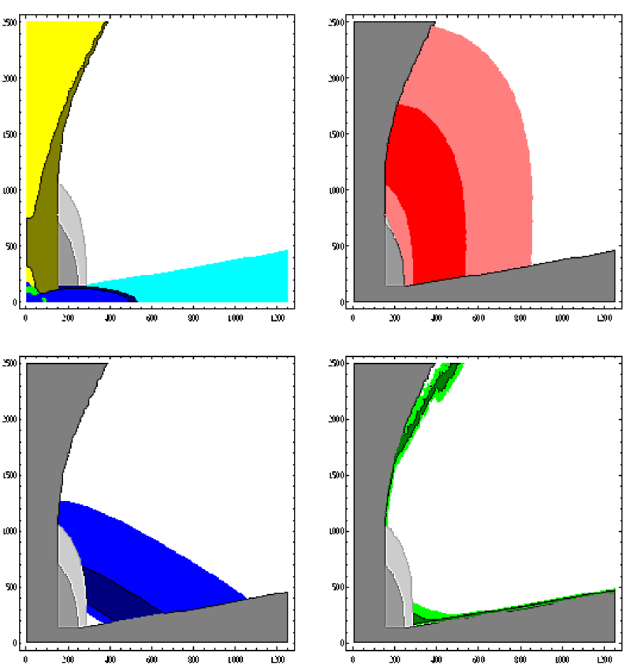
$m_{1/2}$

Figure 1: Constraints on the $(m_{1/2},m_{0})$ mSUGRA plane. Top–Left: individual constraints from non–convergent $\mu$ (yellow region), tachyonic $M_{A}$ (green), tachyonic sfermions (blue), light sfermions (dark), light charginos (brown), $\tilde{\chi}_{1}^{0}$ non–LSP (light blue), BR($b\to s\gamma)$ (medium grey) and light $h$ boson (light and medium grey). The three other plots are for the $1\sigma$ (dark colors) and $2\sigma$ (light colors) “evidence” for, the Higgs boson (but with larger error bars, Top–Right), $(g_{\mu}-2)$ (Bottom–Left) and the Dark Matter (Bottom–Right).

Let us now come to the positive indications for SUSY which are shown in colors in the three other panels of Fig. 1. The “Obelix menhir” (dark red) in the top–right frame corresponds to the region where the lightest $h$ boson mass lies in the range 113 GeV $\leq M_{h}\leq 117$ GeV. It extends from $m_{1/2}$ values below 550 GeV for $m_{0}\raisebox{-3.69899pt}{~{}\shortstack{$<$ \\ [-0.07cm] $\sim$}}~{}1$ TeV down to $m_{1/2}\sim 300$–$200$ GeV for larger $m_{0}$, with upper contour at $m_{0}=1.7$ TeV. For larger values of $m_{0}$ and $m_{1/2}$ the top squarks are very heavy and push $M_{h}$ beyond the 117 GeV limit. One notices that the $M_{h}$ constraint is satisfied in a large region of mSUGRA parameter space, since a variation of the $h$ boson mass of a few GeV leads to a variation of $m_{1/2}$ of several hundred GeV. This is due to the logarithmic dependence on the stop masses, which in turn are mainly driven by $m_{1/2}$. Since the theoretical error on $M_{h}$ [from higher order loop corrections, as well as from a shift of $M_{t}$ by a few GeV within the experimental error, etc..] are expected to be of the order of a few GeV, we display for illustration the effect of including an additional uncertainty of $\pm 2$ GeV on the $h$ boson mass which varies then in range 111 GeV $\leq M_{h}\leq 119$ GeV (light red area). As can be seen, the impact is very large and values $m_{0}\sim 2$ TeV and $m_{1/2}\raisebox{-3.69899pt}{~{}\shortstack{$<$ \\ [-0.07cm] $\sim$}}~{}0.8$ TeV could be reached [this point has also been realized recently, see Ref. [78] for instance]. Some caution is therefore needed when analyzing the consequences of a “115 GeV $h$ boson” for the allowed mSUGRA parameter space.

In the blue regions of the bottom–left frame of Fig. 1 the contribution of SUSY particles to the anomalous magnetic moment of the muon is within two standard deviations (light blue) and one standard deviation(dark blue) from the central value of the measurement made by the Brookhaven experiment, eq. (25). The $2\sigma$ area extends from values $m_{0}\raisebox{-3.69899pt}{~{}\shortstack{$<$ \\ [-0.07cm] $\sim$}}~{}1.2$ TeV for small $m_{1/2}$ to the boundary where the neutralino $\tilde{\chi}_{1}^{0}$ is not the LSP for large values, $m_{1/2}\sim 1$ TeV, except for a little corner with $m_{1/2}\sim m_{0}\sim 250$ GeV, where the SUSY contribution exceeds the $2\sigma$ upper bound. In this area, charginos and smuons have relatively small masses and can give too large a contribution to $(g_{\mu}-2)$. The $1\sigma$ constraint is significantly more severe: a large amount of the upper part of the $2\sigma$ area [where charginos/smuons are too heavy to contribute] and a smaller area of the lower part [where charginos and smuons are too light and generate too large a contribution] are cut away.

Finally, the light green bands in the bottom–right frame correspond to the regions where the LSP neutralino cosmological relic density is in the required range, $0.025\leq\mbox{$\Omega_{\tilde{\chi}_{1}^{0}}h^{2}$}\leq 0.5$. The narrow band slightly above the non $\tilde{\chi}_{1}^{0}$ LSP boundary is the region where $\tilde{\tau}_{1}$ is almost degenerate with the neutralino $\tilde{\chi}_{1}^{0}$, and $\tilde{\tau}_{1}$$\tilde{\chi}_{1}^{0}$  as well as $\tilde{\tau}_{1}\tilde{\tau}_{1}$ co–annihilation is efficient enough to reduce the relic density. The region below $m_{1/2}\raisebox{-3.69899pt}{~{}\shortstack{$<$ \\ [-0.07cm] $\sim$}}~{}400$ GeV and small $m_{0}$ is the bino–like LSP region, where both the LSP and the $\tilde{\tau}_{1}$ are light enough for the annihilation $\tilde{\chi}_{1}^{0}$$\tilde{\chi}_{1}^{0}$$\to\tau^{+}\tau^{-}$ cross section, through $t$–channel $\tilde{\tau}_{1}$ exchange, to be sizeable. The area near the EWSB boundary is again the focus–point region where the $\tilde{\chi}_{1}^{0}$ has a significant higgsino component, i.e. has sizeable couplings to massive gauge bosons, making the annihilation into $WW,ZZ$ efficient. Very close to the “no EWSB” region the $\tilde{\chi}_{1}^{0}$ is higgsino–like and is therefore almost degenerate with the lightest chargino and next–to–lightest neutralino, in which case higgsino co–annihilation takes place. The relic density can then even fall below its lower bound. Note that we did not yet reach the regime where the $s$–channel pseudoscalar Higgs boson poles play an important role, although we have a relatively large value of $\tan\beta$. We also show the regions where the cosmological relic density is more constrained, $0.1\raisebox{-3.69899pt}{~{}\shortstack{$<$ \\ [-0.07cm] $\sim$}}~{}\mbox{$\Omega_{\tilde{\chi}_{1}^{0}}h^{2}$}\raisebox{-3.69899pt}{~{}\shortstack{$<$ \\ [-0.07cm] $\sim$}}~{}0.3$ (dark green). The areas become narrower, in particular the bino–like $\tilde{\chi}_{1}^{0}$ and the focus point regions, but there is no qualitative change from what was discussed above.

$\tan\beta=40\ ,\ A_{0}=0\ ,\ {\rm sign}(\mu)>0$

$m_{0}$

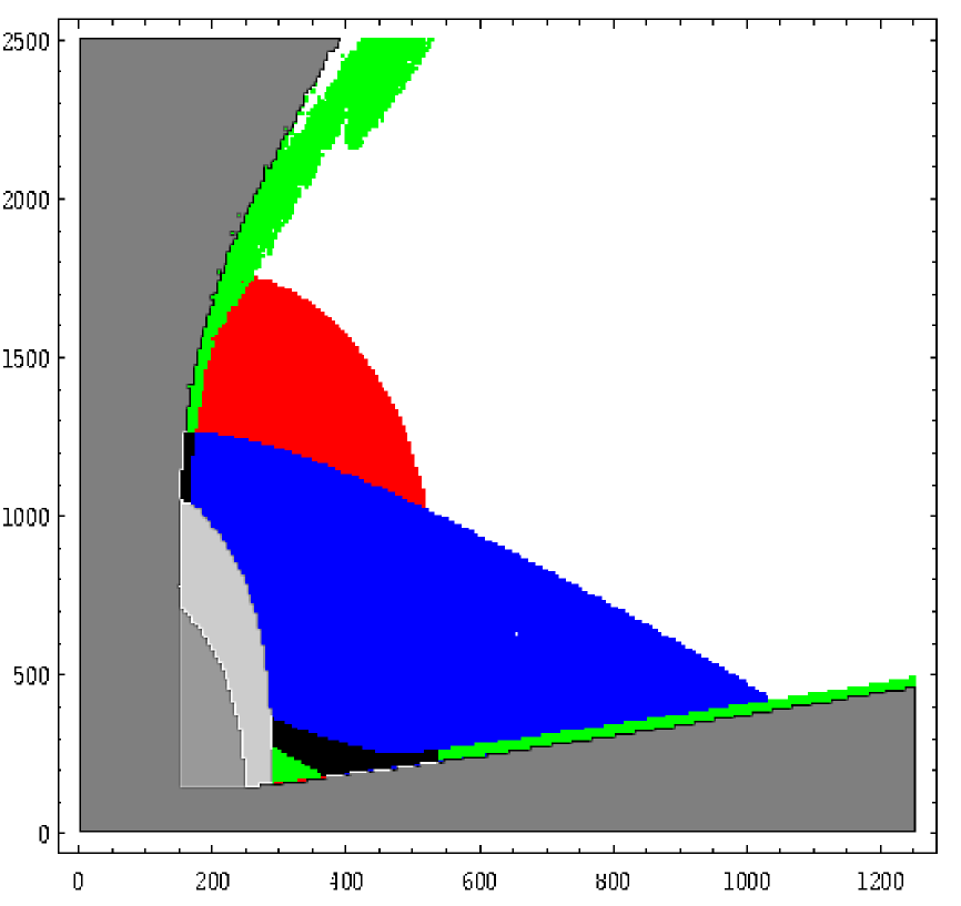
$m_{1/2}$

Figure 2: Constraints on the $(m_{1/2},m_{0})$ mSUGRA plane for $\tan\beta=40$, $A_{0}=0$ and sign$(\mu)>0$. The grey areas are those excluded by the requirement of EWSB breaking and limits on SUSY particle masses (darker grey), BR($b\to s\gamma)$ (medium grey) and $M_{h}>113$ GeV (light and medium grey). The colors are for the “evidence” for the Higgs boson (red), the $(g_{\mu}-2)$ (blue) and Dark Matter (green).

Fig. 2 summarizes the situation when all the constraints as well as the $2\sigma$ “evidence” from the LEP2 lightest $h$ boson, the $(g_{\mu}-2)$ deviation and the neutralino cosmological relic density are superimposed. [Note that some of these colored areas overlap as can be inferred from Figs. 1; we refrained from allocating different colors for these common regions, since one can deduce them by continuing the boundaries up to the dark region which is the intersection of all three areas]. As can be seen, the region excluded by theoretical and experimental considerations is still relatively modest. There are large areas of the parameter space where one can accommodate a $\sim 115$ GeV $h$ boson and a SUSY explanation of the $(g_{\mu}-2)$ deviation. On the other hand, the area where the neutralino LSP is a good Dark Matter candidate is fairly small for this value of $\tan\beta$. The areas (in black) where all of the three requirements are met are rather tiny and include only a part of the region with a light bino LSP neutralino and a very small part of the focus point region, the remaining pieces being removed by the $(g_{\mu}-2)$ or Higgs boson constraints. Using the more constrained scenario with a narrower range for $\Omega_{\tilde{\chi}_{1}^{0}}h^{2}$ and $1\sigma$ errors for $(g_{\mu}-2)$, would have collapsed the overlap region to a narrow strip in the $\mbox{$\tilde{\chi}_{1}^{0}$}-\tilde{\tau}_{1}$ co–annihilation region, with 420 GeV $\leq m_{1/2}\leq$ 520 GeV. The lower bound on $m_{1/2}$ then comes from the upper bound on $(g_{\mu}-2)$, and the upper bound on $m_{1/2}$ results from the upper bound on $M_{h}$.

$\tan\beta=5,\,A_{0}=-1\,{\rm TeV},\,{\rm sign}(\mu)>0$              $\tan\beta=10,\,A_{0}=0,\,{\rm sign}(\mu)>0$
$m_{0}$
                                                                                                                                              $m_{1/2}$

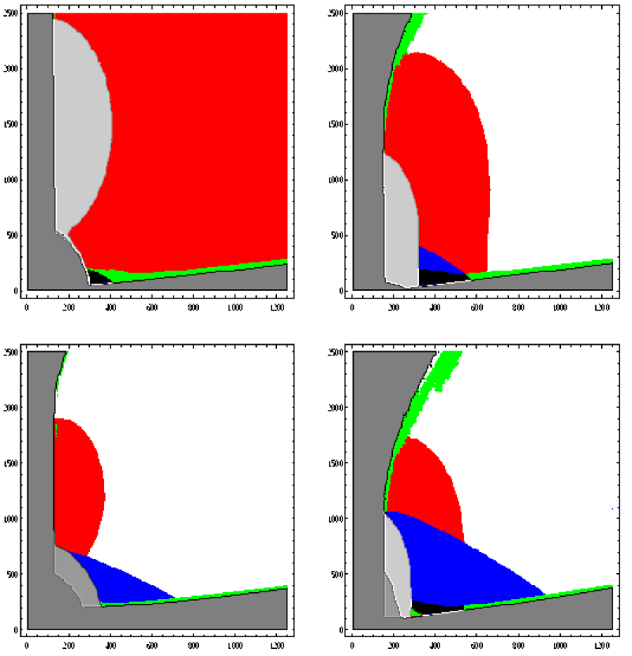
$\tan\beta=20,\,A_{0}=-1\,{\rm TeV},\,{\rm sign}(\mu)>0$               $\tan\beta=30,\,A_{0}=0,\,{\rm sign}(\mu)>0$

Figure 3: Constraints on the $(m_{1/2},m_{0})$ mSUGRA plane for values of $\tan\beta<40$, $A_{0}=0$ or -1 TeV and sign$(\mu)>0$. The grey areas are those excluded by the requirement of EWSB breaking and limits on SUSY particle masses (darker grey), BR($b\to s\gamma)$ (medium grey) and $M_{h}>113$ GeV (light and medium grey). The colors are for the “evidence” for the Higgs boson (red), $(g_{\mu}-2)$ (blue) and Dark Matter (green).

$\tan\beta=45,\,A_{0}=-1\,{\rm TeV},\,{\rm sign}(\mu)>0$               $\tan\beta=50,\,A_{0}=0,\,{\rm sign}(\mu)>0$
$m_{0}$
                                                                                                                                              $m_{1/2}$

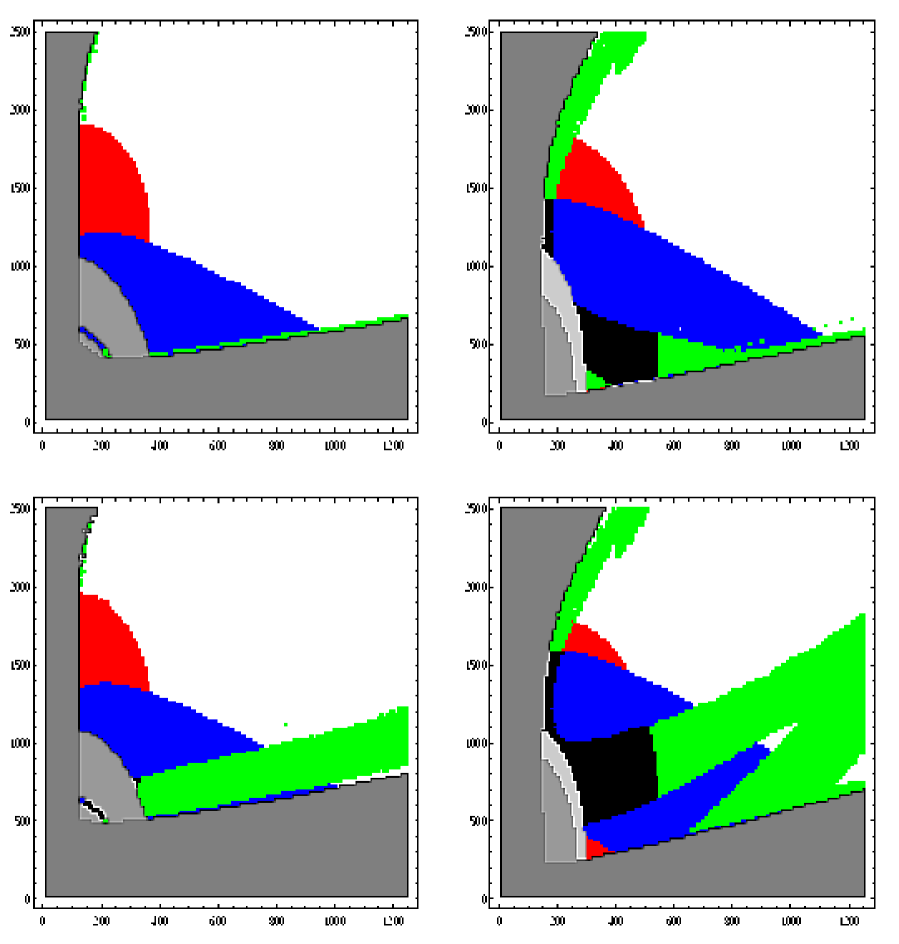
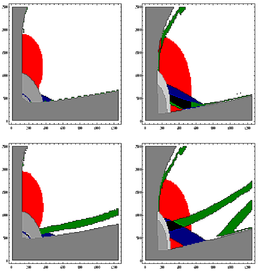
$\tan\beta=55,\,A_{0}=-1\,{\rm TeV},\,{\rm sign}(\mu)>0$               $\tan\beta=60,\,A_{0}=0,\,{\rm sign}(\mu)>0$

Figure 4a: Constraints on the $(m_{1/2},m_{0})$ mSUGRA plane for values of $\tan\beta>40$, $A_{0}=0$ or -1 TeV and sign$(\mu)>0$. The grey areas are those excluded by the requirement of EWSB breaking and limits on SUSY particle masses (darker grey), BR($b\to s\gamma)$ (medium grey) and $M_{h}>113$ GeV (light and dark grey). The colors are for the “evidence” for the Higgs boson (red), and the $(g_{\mu}-2)$ (blue) and Dark Matter (green).

$\tan\beta=45,\,A_{0}=-1\,{\rm TeV},\,{\rm sign}(\mu)>0$               $\tan\beta=50,\,A_{0}=0,\,{\rm sign}(\mu)>0$
$m_{0}$
                                                                                                                                              $m_{1/2}$

$\tan\beta=55,\,A_{0}=-1\,{\rm TeV},\,{\rm sign}(\mu)>0$               $\tan\beta=60,\,A_{0}=0,\,{\rm sign}(\mu)>0$

Figure 4b: As Fig. 4a, except that we have used the $1\sigma$ range for $(g_{\mu}-2)$ and the tighter constraint (31) on $\Omega_{\tilde{\chi}_{1}^{0}}h^{2}$.

In Figs. 3 and 4 we show the same $(m_{0},m_{1/2})$ plane for smaller and larger values of $\tan\beta$, respectively, choosing $A_{0}=0$ or $-1$ TeV. The most striking features are as follows:

(i) The region where EWSB does not take place decreases with decreasing $\tan\beta$. In fact, for $\tan\beta\sim 5$ there is no EWSB problem, and the lower limit on $m_{1/2}$ comes from the requirement $m_{\tilde{\chi}_{1}^{\pm}}\simeq 0.75m_{1/2}\raisebox{-3.69899pt}{~{}\shortstack{$>$ \\ [-0.07cm] $\sim$}}~{}104$ GeV. In contrast, for $\tan\beta\raisebox{-3.69899pt}{~{}\shortstack{$>$ \\ [-0.07cm] $\sim$}}~{}50$ the EWSB constraints rules out a larger part of the parameter space. For very large values, $\tan\beta>60$, the requirement of EWSB becomes extremely strong and most of the parameter space is ruled out. The “no EWSB” region is controlled in part by the top and $b$–quark Yukawa couplings since the RG evolution of $M_{H_{u}}$ and $M_{H_{d}}$ is very sensitive to modifications of $\lambda_{t}$ and $\lambda_{b}$, respectively. Note that EWSB with $\tan\beta>1$ requires $m^{2}_{H_{u}}<m^{2}_{H_{d}}$ at the weak scale, which in turn requires $\lambda_{b}\raisebox{-3.69899pt}{~{}\shortstack{$<$ \\ [-0.07cm] $\sim$}}~{}\lambda_{t}$, leading to an upper bound on $\tan\beta$. The SUSY radiative corrections to $m_{b}$ play an important role here. For positive values of $\mu$, the radiatively corrected $b$–mass, and thus $\lambda_{b}(M_{Z})$, is smaller and the problem is postponed to larger $\tan\beta$. For $\mu<0$, the situation worsens and one reaches the no–EWSB regime for smaller values of $\tan\beta$. A resummation of these corrections, as performed in our analysis [38], is therefore crucial for an accurate treatment of scenarios with very large $\tan\beta$. The no–EWSB region is also smaller for sizable (and negative) values of the mixing parameter $A_{0}$ which enters the RGEs of the Higgs boson masses, the stop/sbottom masses and the SUSY radiative corrections to $m_{b}$ and $m_{t}$.

(ii) The region where the $\tilde{\chi}_{1}^{0}$ is not the LSP decreases with smaller $\tan\beta$, since the mixing in the $\tilde{\tau}$ sector is proportional to $\mu\tan\beta$, so that the splitting between the two stau masses $m_{\tilde{\tau}_{1}}$ and $m_{\tilde{\tau}_{2}}$ becomes smaller. The net effect is that $\tilde{\tau}_{1}$ becomes heavier, for given values of $m_{0}$ and $m_{1/2}$. On the other hand, taking $A_{0}=-1$ TeV increases the value of $|\mu|$ as determined by EWSB, due to the same RGE effect that decreases the “no EWSB” region. This increases $\tilde{\tau}$ mixing and thus reduces $m_{\tilde{\tau}_{1}}$, thereby extending the region where $\tilde{\chi}_{1}^{0}$ is not the LSP.

(iii) The $b\to s\gamma$ constraint is more restrictive for larger $\tan\beta$ values, although it is still not very constraining in the region of parameter space favored by the “115 GeV Higgs boson” and the deviation in $(g_{\mu}-2)$. It also becomes stronger when $A_{0}$ is sizable (and negative), since this reduces $m_{\tilde{t}_{1}}$. For example, in the bottom–left panel in Fig. 3 the $b\rightarrow s\gamma$ constraint excludes the entire region capable of explaining the $(g_{\mu}-2)$ anomaly, so that no overlap region exists even at the 2 $\sigma$ level. The $\Delta\rho$ [and CCB] constraint also becomes more relevant for the small $\tan\beta$ and large $-A_{0}$, again due to the possibly large mass splitting between the two top squarks. However, the region where $\Delta\rho$ is too large is already ruled out by the $b\to s\gamma$ [and $M_{h}$] constraint.

(iv) For small $\tan\beta$ one needs a large mixing in the stop sector [and thus a sizable and negative $A_{0}$] to maximize the $h$ boson mass and to satisfy the bound $M_{h}>113$ GeV. This is true, for example, for $\tan\beta=5$ [top–left frame in Fig. 3]. Even with large stop mixing, $M_{h}$ cannot exceed 117 GeV, so that the whole parameter space is filled by the $M_{h}\sim 115\pm 2$ GeV “evidence”. For increasing $\tan\beta$ [which leads to an increase of $M_{h}$], these areas become smaller and smaller, until one reaches values $\tan\beta\raisebox{-3.69899pt}{~{}\shortstack{$>$ \\ [-0.07cm] $\sim$}}~{}20$ where the maximal value of $M_{h}$ reaches a plateau, as is well known. Note that the mixing changes the form of the red area since $M_{h}$ is maximal for $|A_{t}|\simeq\sqrt{6m_{\tilde{t}_{1}}m_{\tilde{t}_{2}}}$ [the so–called maximal mixing scenario]; for a fixed value of $A_{t}$, $M_{h}$ decreases for larger or smaller stop masses which are controlled by $m_{0}$ and $m_{1/2}$. It is curious to note that for $\tan\beta=5$, $A_{0}<0$ is crucial for allowing a small overlap region where all positive “indications” can be explained [at the $2\sigma$ level, at least], whereas for $\tan\beta=20$ taking $A_{0}=-1$ TeV removes the overlap region that is present for $A_{0}=0$; as noted in (ii), the constraint that $\tilde{\chi}_{1}^{0}$ is the LSP also plays an important role here.

(v) The area where the contribution of SUSY particles allows an explanation of the deviation of the $(g_{\mu}-2)$ from the Brookhaven result is also very sensitive to the value of $\tan\beta$. For $\tan\beta\sim 5$ and $A_{0}$ near zero, the contribution of chargino and smuon loops is not sufficient, except in regions excluded by the other constraints. [We stress again that no point for $\mu<0$ can comply with this constraint]. For larger values of $\tan\beta$, the $(g_{\mu}-2)$ domain becomes larger and for $\tan\beta\raisebox{-3.69899pt}{~{}\shortstack{$>$ \\ [-0.07cm] $\sim$}}~{}40$, values of $m_{1/2}$ or $m_{0}$ in excess of 1 TeV are still compatible [within $2\sigma$] with the central Brookhaven result. We also note that $(g_{\mu}-2)$ is less sensitive to $A_{0}$ than the $b\rightarrow s\gamma$ constraint is. In the former case the sensitivity is only due to the increased value of $|\mu|$ required by EWSB, while the latter constraint is directly sensitive to $A_{t}$ through the $\tilde{t}$ mass matrix, as explained above. Nevertheless changing $A_{0}$ from 0 to $-1$ TeV significantly reduces the values of $m_{0}$ and $m_{1/2}$ required to explain the deviation in $(g_{\mu}-2)$, in order to compensate for the increase of $|\mu|$.

(vi) The region where the $\tilde{\chi}_{1}^{0}$ LSP is required to make the Dark Matter in the universe is also very sensitive to the values of $\tan\beta$ and $A_{0}$. For small $\tan\beta$, the regions with light bino–like LSP and the mixed gaugino–higgsino LSP [focus–point] are smaller; the latter is even absent for $\tan\beta\sim 5$, or for $A_{0}=-1$ TeV. If $\tan\beta\raisebox{-3.69899pt}{~{}\shortstack{$>$ \\ [-0.07cm] $\sim$}}~{}20$, this latter choice of $A_{0}$ also brings the light bino LSP–like region in conflict with the $b\to s\gamma$ constraint, which becomes more severe when $A_{0}$ is reduced below 0, as discussed in (iii). [Note that for $\tan\beta\sim 5$, there is a region where the required value of $\Omega_{\tilde{\chi}_{1}^{0}}h^{2}$ is attained due to $\mbox{$\tilde{\chi}_{1}^{0}$}-\tilde{t}_{1}$ co–annihilation; however, this region is excluded by the $h$ boson mass constraint.] For very large $\tan\beta$ values, the bino–like region becomes much wider, due to reduced $\tilde{\tau}_{1}$ mass and larger Higgs exchange contributions. Moreover, the mixed or higgsino–like region increases in size, since the focus–point scenario is easier to realize at large $\tan\beta$. For $\tan\beta\raisebox{-3.69899pt}{~{}\shortstack{$>$ \\ [-0.07cm] $\sim$}}~{}50$, there are additional domains where $\Omega_{\tilde{\chi}_{1}^{0}}h^{2}$ is in the interesting range, the regions near the pseudoscalar $A$ boson or scalar $H$ boson $s$–channel poles. As discussed previously, for $\tan\beta\gg 1$, $M_{A}$ [and thus also $M_{H}$] become smaller, and their Yukawa couplings to $b$ quarks and $\tau$ leptons [proportional to $\tan\beta$] are strongly enhanced. The resulting large $\tilde{\chi}_{1}^{0}\tilde{\chi}_{1}^{0}\to b\bar{b},\tau^{+}\tau^{-}$ annihilation cross sections reduce the relic density to the required level. Note that with our treatment of the QCD correction to the bottom Yukawa coupling, these Higgs pole regions open up only for values $\tan\beta\raisebox{-3.69899pt}{~{}\shortstack{$>$ \\ [-0.07cm] $\sim$}}~{}50$ in agreement with the recent analyses performed in Ref. [14]. Moreover, the corrections to the physical Higgs masses are of some importance here. The running $A$ and $H$ masses are very close to each other in this region of parameter space, but these corrections decrease $M_{A}$ and increase $M_{H}$, leading to a mass splitting of 10% or more for $\tan\beta=60$. This is larger than the width of these Higgs bosons, which amounts to typically 4% of their mass. $H-$exchange still does not lead to a separate favored region in our scans, due to the $P-$wave suppression, but the large Higgs mass splitting increases the width of the cosmologically favored region. As a result, even the $1\sigma$ overlap region becomes quite sizable for $\tan\beta\raisebox{-3.69899pt}{~{}\shortstack{$>$ \\ [-0.07cm] $\sim$}}~{}50$ and $A_{0}=0$, as shown in the right panels in Fig. 4b.

We now discuss, for the choice $\tan\beta=40$ and $A_{0}=0$, the effect of using different top and bottom quark mass input values, approximately $1~{}\sigma$ and $2\sigma$ higher or lower than the central experimental values, $M_{t}\sim 175\pm 5$ GeV and $\overline{m}_{b}(\overline{m}_{b})=4.25\pm 0.125$ GeV; see Fig. 5. For smaller top quark mass, $M_{t}=170$ GeV, the region where EWSB does not occur becomes much larger. The $M_{h}$ constraint becomes also much more severe; one needs significantly heavier stops, and hence larger values of $m_{0}$ and/or $m_{1/2}$, to obtain a sufficiently large value of $M_{h}$. The $(g_{\mu}-2)$ domain remains almost the same, since in the relevant region of parameter space the value of $|\mu|$ required by EWSB is only slightly reduced by this reduction of the top mass. On the other hand, the DM region, and in particular the mixed higgsino–gaugino region, becomes wider. For larger $M_{t}$ the trend is reversed: the region where EWSB does not occur and the one with large higgsinos–gaugino mixing almost disappear. The Higgs mass constraints become less severe, while the domain where 113 GeV $\leq M_{h}\leq$ 117 GeV is reduced.

$M_{t}=170\,{\rm GeV}\ ,\ \bar{m}_{b}(\bar{m}_{b})=4.24\,{\rm GeV}$             $M_{t}=180\,{\rm GeV}\ ,\ \bar{m}_{b}(\bar{m}_{b})=4.24\,{\rm GeV}$
$m_{0}$
                                                                                                                                              $m_{1/2}$

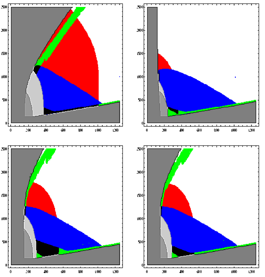
$M_{t}=174.3\,{\rm GeV},\ \bar{m}_{b}(\bar{m}_{b})=4.5\,{\rm GeV}$             $M_{t}=174.3\,{\rm GeV},\,\bar{m}_{b}(\bar{m}_{b})=4.0\,{\rm GeV}$

Figure 5: Constraints on the $(m_{1/2},m_{0})$ mSUGRA plane for $\tan\beta=40$, $A_{0}=0$, sign$(\mu)>0$ and different values of the pole top quark mass $M_{t}$ and $\overline{\rm MS}$ bottom quark mass. The notation is as in Fig. 2.

$M_{\rm EWSB}=0.5\sqrt{m_{\tilde{t}_{1}}m_{\tilde{t}_{2}}}$                                      $M_{\rm EWSB}=2\sqrt{m_{\tilde{t}_{1}}m_{\tilde{t}_{2}}}$
$m_{0}$
                                                                                                                                              $m_{1/2}$

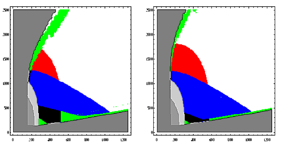
Figure 6: Constraints on the $(m_{1/2},m_{0})$ mSUGRA plane for $\tan\beta=40$, $A_{0}=0$, sign$(\mu)>0$ with different choices of the EWSB scale. The notation is as in Fig. 2

Since for the features related to EWSB an increase of $m_{b}$ is more or less equivalent to an increase of $\tan\beta$, our results for $\bar{m}_{b}=4$ GeV and $\bar{m}_{b}=4.5$ GeV look similar to those where the central value $\overline{m}_{b}(\overline{m}_{b})\sim 4.25$ GeV is kept, but with an input value $\tan\beta\sim 37$ and $\sim 44$, respectively. One sees that in this case, the changes are rather modest. These modest changes however conspire to produce a significant reduction of the overlap region when $\overline{m}_{b}(\overline{m}_{b})$ is reduced from from 4.5 to 4.0 GeV (bottom panels in Fig. 5). The effect of varying $m_{b}$ would have been more striking for large $\tan\beta\raisebox{-3.69899pt}{~{}\shortstack{$>$ \\ [-0.07cm] $\sim$}}~{}50$, where EWSB and the cosmological relic density become much more sensitive to the $b$–Yukawa coupling. For instance, the regime where it is difficult to realize EWSB is reached for lower values of $\tan\beta$, $\tan\beta\sim 55$, if $\overline{m}_{b}(\overline{m}_{b})\sim 4.5$ GeV is used as an input.

There is a residual scale dependence in our treatment of the MSSM scalar potential, since only the one–loop corrections are fully included. A standard RG improvement of the effective potential does not completelly remove the scale dependence, due to the presence of several a priori unrelated scales.  The effect of varying the scale at which EWSB is realized [i.e. the scale at which the effective one–loop scalar potential is evaluated and the running of the soft SUSY breaking terms is frozen] by a factor of 2 in either direction is displayed in Fig. 6. Here again, except for a small change in the shape of the $M_{h}=115\pm 2$ GeV domain, the most striking change occurs for the area where the cosmological relic density is in the interesting range. Increasing the EWSB scale to $M_{\rm EWSB}=2\sqrt{m_{\tilde{t}_{1}}m_{\tilde{t}_{2}}}$ (right panel) increases the predicted value of $|\mu|$. This reduces the size of the cosmologically favored mixed higgsino–bino region, but leaves the light bino region largely unaffected. On the other hand, the choice $M_{\rm EWSB}=0.5\sqrt{m_{\tilde{t}_{1}}m_{\tilde{t}_{2}}}$ (left panel) leads to a significant reduction of the predicted value of $|\mu|$, and a corresponding decrease of the “no EWSB” area as well as the cosmologically preferred area where the LSP has a significant higgsino component. Moreover, the reduction of $|\mu|$ leads to a reduction of the masses of the heavy Higgs bosons. This significantly increases the cosmologically preferred region where the LSP is bino–like, and hence also increases the overlap region, as can be seen by comparing the left panel in Fig. 6 with Fig. 2. In addition a new feature occurs: the opening of the region where the $s$–channel pseudoscalar $A$ boson pole starts to play a role in the LSP annihilation cross section. For the present choice of the scale [and $\tan\beta$] this region is still rather tiny, a small line parallel to the co–annihilation region. If the scale is reduced to much lower values, e.g. to $M_{\rm EWSB}=M_{t}$ or $M_{Z}$, this area would have been much more sizeable. However, in this case, the requirement of proper electroweak symmetry breaking will exclude large portions of the parameter space.

No SUSY RC to sparticle masses                   No SUSY RC to (s)particle masses.
$m_{0}$
                                                                                                                                              $m_{1/2}$

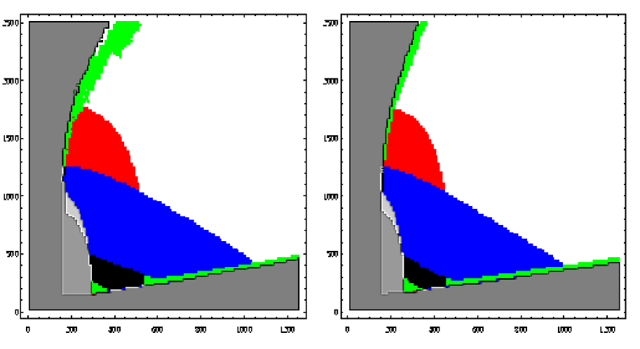
Figure 7: Constraints on the $(m_{1/2},m_{0})$ mSUGRA plane for $\tan\beta=40$, $A_{0}=0$, sign$(\mu)>0$ when certain radiative corrections are not included. In the left panel we have omitted corrections to all superparitcle masses, and in the right panel we have in addition neglected corrections to heavy fermion masses. The notation is as in Fig. 2.

Finally, we show in Fig. 7 the effect of the SUSY radiative corrections on the parameter space. In the left panel we have switched off all radiative corrections to the masses of SUSY particles [neutralinos, charginos, gluinos and squarks]. This has almost no effect on the Higgs boson and $(g_{\mu}-2)$ constraints, but the “light” bino–like LSP DM region becomes slightly larger. The largest effect is the increase of the region excluded by the $b\to s\gamma$ constraint: the radiative corrections tend to increase the stop and chargino masses, so switching them off makes these sparticles lighter, leading to larger contributions to the $b\to s\gamma$ decay width.

The impact of the SUSY radiative corrections to the top and bottom quark masses [right panel] is slightly more important. These corrections tend to increase $M_{t}$ relative to the running mass, so switching them off increases the size of the top Yukawa coupling $\lambda_{t}$. This shrinks the “no EWSB” region, as well as the cosmologically favored region where the LSP is higgsino–like. The value of $m_{t}$ that appears in the stop mass matrix, which is the “MSSM” running mass in the notation of Ref. [38], also increases. This shifts the right boundary of the area excluded by the $b\rightarrow s\gamma$ constraint to slightly lower values of $m_{1/2}$. Moreover, the region where 113 GeV $\raisebox{-3.69899pt}{~{}\shortstack{$<$ \\ [-0.07cm] $\sim$}}~{}M_{h}\raisebox{-3.69899pt}{~{}\shortstack{$<$ \\ [-0.07cm] $\sim$}}~{}$ 117 GeV becomes slightly smaller. Since the SUSY radiative corrections tend also to decrease the bottom quark mass $m_{b}$, their removal will lead to an increase of $\lambda_{b}$, and hence to a more extended region where the cosmological relic density is in the interesting range, as is the case for larger $\bar{m}_{b}$ values [Fig. 5] or larger values of $\tan\beta$ [Fig. 4]. Finally, we note that switching off all two–loop terms in the RGE would dramatically extend the “no EWSB” region, as also pointed out in Ref. [44].

4. Sparticle and Higgs Production in e⁺e^- Collisions

In this section we will discuss the prospects for producing SUSY particles and heavier Higgs bosons at future linear $e^{+}e^{-}$ colliders with center of mass energies between 500 GeV and 1.2 TeV, in the context of the mSUGRA model. We first list the production processes that we will analyze and then discuss the regions of the $(m_{1/2},m_{0})$ parameter space, for various input values of $\tan\beta$ and $A_{0}$, in which these processes are accessible. For completeness, analytical expressions for the relevant total production cross sections are given in the Appendix.

In this exploratory study we will assess the accessibility of certain production modes simply through the corresponding total cross section, without performing any background studies. However, in most cases the clean experimental environment offered by $e^{+}e^{-}$ colliders should indeed permit discovery of a certain mode, given a sample of a few dozen events. Difficulties might arise in some narrow regions of parameter space, which we will point out in the following discussion.

4.1 Production processes

In our study, we will consider the following production processes:

$${\rm Pair~{}production~{}of~{}the~{}lightest~{}charginos}:\ \ e^{+}e^{-}\to\tilde{\chi}_{1}^{+}\tilde{\chi}_{1}^{-}.$$ (33)

This proceeds through $s$–channel photon and $Z$ boson exchange as well as $t$–channel sneutrino exchange. For higgsino–like charginos, $M_{2}\gg|\mu|$, or heavy sneutrinos, only the $s-$channel diagrams contribute substantially. Note that the $Z$ boson couples more strongly to the wino components of $\tilde{\chi}_{1}^{\pm}$ than to its higgsino component, and the $t$–channel $\tilde{\nu}_{e}$ exchange contributes with opposite sign as the $s-$channel diagrams. The cross section is thus maximal for heavy sneutrino and $M_{2}\ll|\mu|$. For small $m_{\tilde{\nu}_{e}}$, which corresponds to small $m_{0}$, the $t$–channel contribution can reduce the cross section significantly. If the chargino is higgsino–like, the cross section becomes insensitive to $m_{\tilde{\nu}}$, since the $\tilde{\nu}e\tilde{\chi}_{1}^{\pm}$ couplings are zero in this limit. We thus see that the production cross section for fixed chargino mass can vary significantly across the parameter space, but it is always rather large, so that masses close to the kinematical threshold should be accessible. The only exception can occur in the very higgsino–like region, where the $\tilde{\chi}_{1}^{\pm}-\mbox{$\tilde{\chi}_{1}^{0}$}$ mass difference becomes small. In the most extreme case one may have to rely on events with additional hard photon to suppress backgrounds [80]. However, we found that this can happen only in a very narrow strip near the “no EWSB” boundary, where the LSP relic density is below the currently favored range.

The $\tilde{\chi}_{1}^{\pm}$ decay pattern depends on its mass difference to the LSP, as well as to sleptons and charged Higgs bosons. If the lighter chargino is the lightest charged sparticle [generally for $m_{0}\raisebox{-3.69899pt}{~{}\shortstack{$>$ \\ [-0.07cm] $\sim$}}~{}m_{1/2}$], it mostly decays into $\tilde{\chi}_{1}^{0}$ plus a real or virtual $W$ boson which in turn decays into $f\bar{f}^{\prime}$ pairs with well–known branching ratios. For smaller ratio $m_{0}/m_{1/2}$ real or virtual slepton exchange contributions become important, in some cases leading to a leptonic branching ratio near 100%. There is a very narrow strip in parameter space where $\tilde{\chi}_{1}^{\pm}\rightarrow\tilde{\nu}_{\ell}\ell^{\pm}\ (\ell=e,\mu,\tau)$ has a large branching ratio but the charged lepton is very soft. Here one might again have to require the existence of an additional hard photon in the event to suppress backgrounds. However, in this case charged slepton pair production is also accessible. There are also regions where $\tilde{\chi}_{1}^{\pm}$ decays predominantly into $\tau^{\pm}\nu_{\tau}\mbox{$\tilde{\chi}_{1}^{0}$}$, either because the $\tilde{\tau}_{1}$ mass is reduced compared to the other slepton masses [this happens at large $\tan\beta$ [81]], or because L–R mixing greatly enhances the $\tilde{\chi}_{1}^{\pm}\tilde{\tau}_{1}\nu_{\tau}$ couplings relative to the corresponding couplings of $\tilde{e}_{1}\simeq\tilde{e}_{R}$ and $\tilde{\mu}_{1}\simeq\tilde{\mu}_{R}$; this latter effect can become important already for moderate values of $\tan\beta$, if $m_{1/2}/2\raisebox{-3.69899pt}{~{}\shortstack{$<$ \\ [-0.07cm] $\sim$}}~{}m_{0}\raisebox{-3.69899pt}{~{}\shortstack{$<$ \\ [-0.07cm] $\sim$}}~{}m_{1/2}$ [82]. Finally, for very large values of $\tan\beta$, charged Higgs boson exchange contributions can also play a role, again leading to an enhanced branching fraction for the $\tau$ mode. However, a large or even dominant branching ratio into $\tau\nu_{\tau}\mbox{$\tilde{\chi}_{1}^{0}$}$ is not expected to significantly degrade the mass reach for $\tilde{\chi}_{1}^{+}\tilde{\chi}_{1}^{-}$ production at $e^{+}e^{-}$ colliders, which should be very close to the kinematical limit [as at LEP]. To the contrary, the measurement of $\tilde{\chi}_{1}^{\pm}$ decay branching ratios might allow one to extract information about (s)particles that are too heavy to be pair–produced.

$${\rm Production~{}of~{}the~{}lightest~{}neutralinos}:\ \ e^{+}e^{-}\to\tilde{\chi}_{1}^{0}\tilde{\chi}_{2}^{0}.$$ (34)

This process is mediated by $s-$channel $Z-$boson exchange and $t-$ and $u-$channel $\tilde{e}_{L},\tilde{e}_{R}$ exchanges. In the gaugino limit, $|\mu|\gg M_{1},M_{2}$, the $Z$ boson coupling to neutralinos vanishes and only the $t$ and $u$–channel contributions are present. The latter will be suppressed for high selectron masses, i.e. for large $m_{0}$; however, $m_{0}\gg m_{1/2}$ also generally implies that $|\mu|$ is not so large, so the size of the $Z-$exchange contribution increases in this region. In the extreme higgsino limit, only the $Z$ boson exchange contribution will survive since the $e\tilde{e}\tilde{\chi}_{1,2}^{0}$ couplings are ${\cal O}(10^{-5})$. Except in the extreme higgsino limit, the cross section is much smaller than the cross section for chargino pair production; however, as will be shown later, the anticipated high luminosity should ensure a detectable signal over most of the kinematically accessible parameter space.

As well known [83, 81] the $\tilde{\chi}_{2}^{0}$ branching ratios depend strongly on details of the SUSY particle spectrum. For example, the branching ratio into $\ell^{+}\ell^{-}\mbox{$\tilde{\chi}_{1}^{0}$}$ can vary between nearly 100% and almost zero. The former occurs if $\tilde{\chi}_{2}^{0}\rightarrow\ell^{\pm}\tilde{\ell}^{\mp}_{1}$ is the only 2–body decay mode of $\tilde{\chi}_{2}^{0}$, while the latter situation is e.g. realized if $\tilde{\chi}_{2}^{0}\rightarrow h\tilde{\chi}_{1}^{0}$ is dominant. However, at an $e^{+}e^{-}$ collider hadronic $\tilde{\chi}_{2}^{0}$ decays are as easily detectable as decays into charged leptons. The only potentially difficult scenarios are the extreme higgsino region, where the $\tilde{\chi}_{2}^{0}-\mbox{$\tilde{\chi}_{1}^{0}$}$ mass difference is small [but stays about twice as large as the $\tilde{\chi}_{1}^{\pm}\mbox{$\tilde{\chi}_{1}^{0}$}$ mass difference], or scenarios where $\tilde{\chi}_{2}^{0}$ decays almost exclusively into the invisible mode $\nu\bar{\nu}\mbox{$\tilde{\chi}_{1}^{0}$}$; however, this latter scenario is never realized in mSUGRA, given current experimental constraints.

We will not discuss the production of pairs of the next–to–lightest neutralinos, $e^{+}e^{-}\to\tilde{\chi}_{2}^{0}\tilde{\chi}_{2}^{0}$, since in mSUGRA this process leads to the same reach at $e^{+}e^{-}$ colliders as $\tilde{\chi}^{\pm}_{1}$ pair production; the approximate equality $m_{\tilde{\chi}_{2}^{0}}\simeq m_{\tilde{\chi}_{1}^{\pm}}$ holds in both the higgsino and the gaugino limit. However, the neutralino production cross section is smaller due to the absence of the photon exchange channel, and because the $Z$ boson does not couple to neutral SU(2) gauginos. Nor will we consider the production of heavier states, $e^{+}e^{-}\to\tilde{\chi}_{i}^{0}\tilde{\chi}_{j}^{0}$ with $i$ or $j>2$ and $e^{+}e^{-}\to\tilde{\chi}_{i}^{\pm}\tilde{\chi}_{j}^{\mp}$ with $i$ or $j>1$, since these channels cannot extend the overall discovery reach. Of course, one would eventually like to also study these channels in detail in a clean environment.

$${\rm Pair~{}production~{}of~{}charged~{}sleptons}:\ \ e^{+}e^{-}\to\tilde{\ell}^{+}\tilde{\ell}^{-}.$$ (35)

Pairs of SU(2) doublet [“left–”] and singlet [“right–handed”] selectrons are produced via $s$–channel photon and $Z$ boson exchange and the $t$–channel exchange of the four neutralinos $\tilde{\chi}_{i}^{0}$. Since the vector boson couplings to charged slepton current eigenstates are full strength gauge couplings and L–R mixing between selectrons is negligible [for our purposes], the first two channels always contribute. Since the electron Yukawa coupling is tiny, only the exchange of the gaugino–like neutralinos plays a role here. To good approximation the cross section is therefore determined by the sizes of the soft breaking gaugino masses $M_{1}$ and $M_{2}$. In mSUGRA they are related via eq.(1), which leads to $M_{1}\simeq M_{2}/2$ at the weak scale. The value of $|\mu|$ is not relevant here. Moreover, mixed $\tilde{e}_{L}^{\pm}\tilde{e}_{R}^{\mp}$ production is possible through the exchange of neutralinos in the $t-$ or $u-$channel. However, in mSUGRA the overall mass reach in selectron pair production will be determined by $\tilde{e}_{R}$ pair production, since the $\tilde{e}_{R}-\tilde{e}_{L}$ mass difference can be sizable.

The production of second and third generation charged sleptons only proceeds through $s-$channel $\gamma$ and $Z$ boson exchange. Since the mixing in the $\tilde{\tau}$ sector can be large, it has to be included in the $Z\tilde{\tau}\tilde{\tau}$ couplings; in this case we will only consider the production of the lighter $\tilde{\tau}$ states, $e^{+}e^{-}\to\tilde{\tau}_{1}\tilde{\tau}_{1}$, which offers the largest reach. Note that, with the exception of $\tilde{e}_{L}^{\pm}\tilde{e}_{R}^{\mp}$ production, the cross section for the production of sleptons near threshold is strongly suppressed by $\beta^{3}$ factors, $\beta$ being the cms velocity of the sleptons. Therefore only slepton masses up to several GeV below the kinematical limit can be probed.

The sleptons will mostly decay into their partner leptons and the gaugino–like neutralinos and [if accessible] charginos. Slepton pair production at next–generation $e^{+}e^{-}$ colliders will only be accessible if $m_{0}$ is not very large, away from the “focus–point” region. The gaugino–like neutralinos and charginos will then be the lighter states, since mSUGRA predicts $|\mu|>M_{2}$ unless $m_{0}\gg m_{1/2}$. In particular, for the lighter slepton mass eigenstates the by far dominant decay will be $\tilde{\ell}^{\pm}_{1}\to\ell^{\pm}\tilde{\chi}_{1}^{0}$. If phase space allows it, the heavier left–handed sleptons will decay predominantly into wino–like charginos $\tilde{\chi}_{1}^{\pm}$ or neutralinos $\tilde{\chi}_{2}^{0}$, plus a neutrino or charged lepton, since these decays occur via SU(2) couplings which exceed the U$(1)_{\rm Y}$ couplings responsible for $\tilde{\ell}_{L}\rightarrow\ell\mbox{$\tilde{\chi}_{1}^{0}$}$ decays. In the case of $\tilde{\tau}$ sleptons, both states might be able to decay via the charged current because of L–R mixing. For large $\tan\beta$ the $\tilde{\tau}_{2}$ decay pattern can be rather complicated [84]. The mass reach for $\tilde{\tau}_{1}$ pair production is expected to be a little lower than that for $\tilde{\mu}$ pair production, since the $\tau$ leptons produced in $\tilde{\tau}_{1}\rightarrow\tau\mbox{$\tilde{\chi}_{1}^{0}$}$ will themselves decay, which degrades the visible energy. This becomes of some concern in a narrow strip of parameter space close to the lower bound on $m_{0}$, i.e. near the region excluded by the requirement $\mbox{$m_{\tilde{\chi}_{1}^{0}}$}<m_{\tilde{\tau}_{1}}$. On the other hand, $\tilde{\tau}_{1}$ pair production generally still gives a larger reach in the $(m_{1/2},m_{0})$ plane, since for $\tan\beta\gg 1$, $m_{\tilde{\tau}_{1}}$ is significantly smaller than $m_{\tilde{\mu}_{R}}$. Moreover, the measurement of the polarization of the produced $\tau$ leptons could yield important information about the SUSY model [85].

$${\rm Pair~{}production~{}of~{}sneutrinos}:\ \ e^{+}e^{-}\to\tilde{\nu}\bar{\tilde{\nu}}.$$ (36)

Muon and tau sneutrino pairs are produced only through $s$–channel $Z$–boson exchange. Electron sneutrinos can also be produced through $t$–channel diagrams with the exchange of the [gaugino–like] charginos, which enhances the cross section significantly if $m_{1/2}$ is not too large. All $\tilde{\nu}$ pair production cross sections show the familiar $\beta^{3}$ behavior near threshold.

In mSUGRA the sneutrinos [as well as the “left–handed” charged sleptons] are usually heavier than the SU(2) gauginos. Sneutrinos can thus generally decay through both neutral and charged currents into leptons and gauginos, $\tilde{\nu}\to\nu\tilde{\chi}_{i}^{0}$ and $\tilde{\nu}\to l^{\pm}\tilde{\chi}_{i}^{\mp}$. In the narrow range where $m_{\tilde{\chi}_{1}^{0}}\leq m_{\tilde{\nu}}\leq m_{\tilde{\chi}_{1}^{\pm}},m_{\tilde{\chi}_{2}^{0}}$, which can occur for $m_{1/2}\gg m_{0}$ if the overall SUSY mass scale is rather low so that the negative $D-$term contribution to $m^{2}_{\tilde{\nu}}$ plays a role, the only allowed decay will be the invisible decay into the LSP and a neutrino. However, in mSUGRA such scenarios are excluded by the $h$ mass constraint. Usually this invisible decay is disfavored by the smallness of the U$(1)_{\rm Y}$ gauge coupling.

$${\rm Pair~{}production~{}of~{}stops~{}and~{}sbottoms}:\ \ e^{+}e^{-}\to\tilde{t}_{1}\bar{\tilde{t}}_{1}\ ,\ \tilde{b}_{1}\bar{\tilde{b}}_{1}.$$ (37)

In $e^{+}e^{-}$ collisions, squarks can only be produced through $s$–channel photon and $Z$ boson exchange. In our analysis, we will consider only the pair production of the states $\tilde{t}_{1}$ and $\tilde{b}_{1}$ which are in general significantly lighter than the other squark states, due the large Yukawa couplings of top and bottom quarks. In both cases $L-R$ mixing can affect the coupling to $Z$ bosons, and hence the total cross section [86], but the latter remains sizable unless these processes are kinematically suppressed.

The mixing in the stop sector and the large top quark mass might generate some complications in the decays of $\tilde{t}_{1}$, since the usual two–body squark decays $\tilde{q}\to q\tilde{g},\ q\tilde{\chi}_{i}^{0}$ and $q^{\prime}\tilde{\chi}_{i}^{\pm}$ are kinematically closed for sizable regions of parameter space. In this case, $\tilde{t}_{1}$ decays are dominated by loop induced two–body decay channels [such as the flavor changing decay into a charm quark and the LSP [87]], or by tree–level three–body [$bW\tilde{\chi}_{1}^{0},bH^{+}\tilde{\chi}_{1}^{0}$ or $bl\tilde{l}$] or even four–body [$b\mbox{$\tilde{\chi}_{1}^{0}$}f\bar{f}^{\prime}$ where $f,f^{\prime}$ are massless fermions] decay modes [88]. In contrast, tree–level two–body decays $\tilde{b}_{1}\rightarrow b\tilde{\chi}_{i}^{0}$ decays are always possible at least for $i=1$. As in the case of $\tilde{\tau}$, the decay patterns of the heavier states $\tilde{b}_{2}$ and $\tilde{t}_{2}$ can again be rather complicated [84].

$${\rm Pair~{}production~{}of~{}Higgs~{}bosons}:\ \ e^{+}e^{-}\to AH\ {\rm and}\ H^{+}H^{-}.$$ (38)

If the pseudoscalar Higgs boson $A$ is relatively heavy, $M_{A}\raisebox{-3.69899pt}{~{}\shortstack{$>$ \\ [-0.07cm] $\sim$}}~{}200$ (130) GeV for moderate (large) values of $\tan\beta$, we are in the so–called decoupling regime where the running masses of the heavier Higgs bosons $A,H$ are almost degenerate; for even larger $M_{A}$, the $H^{\pm}$ mass also becomes very similar. In that limit, which is realized for most of the allowed mSUGRA parameter space, the lighter $h$ boson mass reaches its maximal value, $M_{h}\raisebox{-3.69899pt}{~{}\shortstack{$<$ \\ [-0.07cm] $\sim$}}~{}130$ GeV, and $h$ has Standard Model like couplings to fermions and gauge bosons. The pseudoscalar Higgs boson has no tree–level couplings to two gauge bosons. In the decoupling limit, the couplings of $H$ to two massive vector bosons are also strongly suppressed, as is the $ZAh$ coupling. The only significant $2\to 2$ process for the production of the heavier neutral Higgs bosons is thus associated $HA$ production through $Z$ boson exchange in the $s$–channel. The charged Higgs particles can be pair–produced photon and $Z$ boson exchange. These cross sections are sufficiently large [although once again suppressed by $\beta^{3}$ factors near threshold] to allow for the production of detectable quantities of these particles up to almost the beam energy.

If $\tan\beta>\sqrt{\overline{m}_{t}(\overline{m}_{t})/\overline{m}_{b}(\overline{m}_{b})}$ or $M_{A}<2M_{t}$ the heavy neutral Higgs bosons will mainly decay into $b\bar{b}$ and $\tau^{+}\tau^{-}$ pairs [with relative abundance $\sim 9:1$]. For smaller values of $\tan\beta$, decays into $t\bar{t}$ pairs dominate, if kinematically allowed. The charged Higgs bosons will dominantly decay into $tb$ and $\tau\nu$ final states. In some cases decays into SUSY particles [charginos, neutralinos and possibly sleptons and stops; only this last mode can compete with decays into $t\bar{t}$, or with $b\bar{b}$ at large $\tan\beta$] can be possible [89]. These decays will be more difficult to analyze, but in most cases should be clean enough to be detectable at $e^{+}e^{-}$ colliders. [The main background will probably come from the direct pair production of heavier superparticles.]

Of course, the light scalar $h$ boson can be produced [in association with a $Z$ boson, and/or through gauge boson fusion] over the entire mSUGRA parameter space. Detailed studies [90, 91] have shown that detection of this particle is straightforward at an $e^{+}e^{-}$ collider with c.m. energy $\sqrt{s}\raisebox{-3.69899pt}{~{}\shortstack{$>$ \\ [-0.07cm] $\sim$}}~{}250$ GeV even with moderate luminosities, $\int{\cal L}dt\raisebox{-3.69899pt}{~{}\shortstack{$>$ \\ [-0.07cm] $\sim$}}~{}10$ fb^-1. With the high luminosities expected at a linear collider, $\int{\cal L}dt\sim 500$ fb^-1, detailed studies of the profile of this particle can be made already at $\sqrt{s}\raisebox{-3.69899pt}{~{}\shortstack{$<$ \\ [-0.07cm] $\sim$}}~{}500$ GeV: the mass can be measured at the permille level, various couplings to fermions and gauge bosons [which determine the production cross sections and decay branching ratios] can be measured at the percent level, and even the Higgs self–coupling can be measured at the level of $\sim 10-20\%$. In the MSSM these measurements should reveal some deviations from Standard Model predictions for $M_{A}\raisebox{-3.69899pt}{~{}\shortstack{$<$ \\ [-0.07cm] $\sim$}}~{}500$ GeV to 1 TeV. Nevertheless this indirect evidence for the existence of heavier Higgs bosons will have to be confirmed through their direct production.

4.2 Results

In a first step, we will analyze (s)particle production at an $e^{+}e^{-}$ collider with $\sqrt{s}=800$ and an annual luminosity of ${\cal L}=500$ fb${}^{-1}/$yr. This is e.g. expected for the second phase of the TESLA machine [92]. We will consider a given channel to be visible if its total cross section exceeds $\sigma_{\rm min}=0.1$ fb, which means that a sample of 50 signal events per year will be required, with the assumed luminosity [or 100 events with a two years running], to establish discovery. This number should usually be sufficient for discovery in the clean environment offered by $e^{+}e^{-}$ colliders [90, 91].

We will also illustrate the potential of the first phase of the $e^{+}e^{-}$ collider with $\sqrt{s}=500$ GeV and the same luminosity. We will then discuss the increase of the discovery potential if the energy of the collider could be raised to $\sqrt{s}=1.2$ TeV [25]. This could be accomplished either by simply extending the electron and/or positron accelerators, or by increasing the RF power if the cavity modules generate higher gradients than originally envisaged [as is the case for the most recent TESLA cavities]. However, in order to compensate for the $1/s$ drop of most background cross sections with raising c.m. energy, we will require a smaller minimal cross section than in the previous cases, $\sigma_{\rm min}=0.025$ fb. In order to obtain the same number of signal events one would then either have to increase the luminosity [as is the case for the TESLA machine [92] where the luminosity is expected to scale with the energy], or to extend the running period of the machine.

Figs. 8–10 show the regions in the usual $(m_{1/2},m_{0})$ plane where various superparticles and heavy Higgs bosons can be discovered at an $e^{+}e^{-}$ collider with a c.m. energy $\sqrt{s}=800$ GeV and a luminosity $\int{\cal L}dt=500$ fb^-1, for the same values of $\tan\beta$ and $A_{0}$ taken in Figs. 1–3. The grey areas are again those excluded by theoretical and experimental constraints. The colored regions correspond to the following production processes: $e^{+}e^{-}\to\tilde{\chi}_{1}^{0}\tilde{\chi}_{2}^{0}$ (green+red), $e^{+}e^{-}\to\tilde{\chi}_{1}^{+}\tilde{\chi}_{1}^{-}$ (red), $e^{+}e^{-}\to\tilde{\ell}^{+}\tilde{\ell}^{-}$ (blue), $e^{+}e^{-}\to\tilde{\nu}\bar{\tilde{\nu}}$ (purple), $e^{+}e^{-}\to\tilde{t}_{1}\bar{\tilde{t}}_{1}$ (dark blue), $e^{+}e^{-}\to\tilde{b}_{1}\bar{\tilde{b}}_{1}$ (dark green) and the heavy MSSM Higgs boson production $e^{+}e^{-}\to HA$ and $H^{\mp}H^{\pm}$ (yellow). Note that some of these regions are overlapping. For example, in Fig. 8 the chargino and neutralino areas should be extended until the lower boundary where the LSP is not the $\tilde{\chi}_{1}^{0}$, the $\tilde{\tau}$ region includes the sneutrino and Higgs regions, and the sneutrino area includes the Higgs boson region. Moreover, the region where $\mbox{$\tilde{\chi}_{1}^{0}$}\tilde{\chi}_{2}^{0}$ production is accessible always includes the entire $\tilde{\chi}_{1}^{\pm}$ pair production region.

$\tan\beta=40\ ,\ A_{0}=0\ ,\ {\rm sign}(\mu)>0$

$m_{0}$

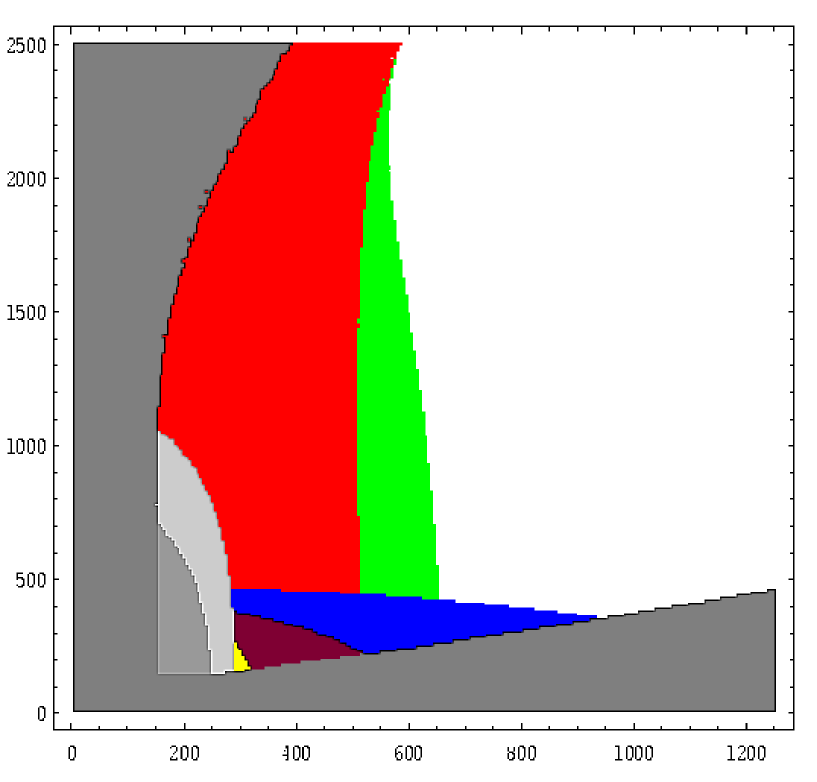
$m_{1/2}$

Figure 8: The $(m_{1/2},m_{0})$ mSUGRA plane where SUSY and Higgs particles can be produced at an $e^{+}e^{-}$ collider with a c.m. energy $\sqrt{s}=800$ GeV. The grey areas are those excluded by theoretical and experimental constraints. The colored regions are those where a given cross section is large enough for the particles to be produced: $\tilde{\chi}_{1}^{0}\tilde{\chi}_{2}^{0}$ (green), $\tilde{\chi}_{1}^{+}\tilde{\chi}_{1}^{-}$ (red), $\tilde{\ell}^{+}\tilde{\ell}^{-}$ (blue), $\tilde{\nu}\bar{\tilde{\nu}}$ (purple), $\tilde{t}_{1}\bar{\tilde{t}}_{1}$ (dark blue), $\tilde{b}_{1}\bar{\tilde{b}}_{1}$ (dark blue) and the heavy MSSM $H,A,H^{\pm}$ bosons (yellow). Note that some of these regions are overlapping.

$\tan\beta=5,\,A_{0}=-1\,{\rm TeV},\,{\rm sign}(\mu)>0$               $\tan\beta=10,\,A_{0}=0,\,{\rm sign}(\mu)>0$
$m_{0}$
                                                                                                                                              $m_{1/2}$

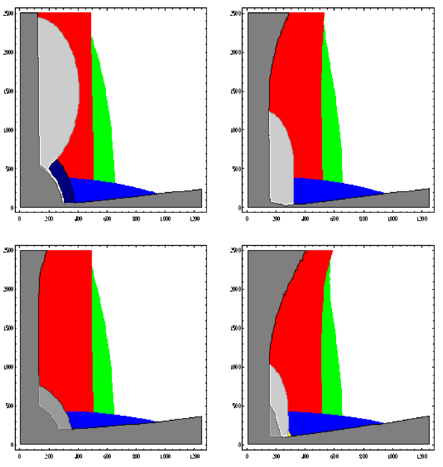
$\tan\beta=20,\,A_{0}=-1\,{\rm TeV},\,{\rm sign}(\mu)>0$               $\tan\beta=30,\,A_{0}=0,\,{\rm sign}(\mu)>0$

Figure 9: The $(m_{1/2},m_{0})$ mSUGRA plane where SUSY and Higgs particles can be produced at an $e^{+}e^{-}$ collider with a c.m. energy $\sqrt{s}=800$ GeV for different values of $\tan\beta<40$ and $A_{0}$ with sign($\mu)>0$. The notation is as in Fig. 8.

$\tan\beta=45,\,A_{0}=-1\,{\rm TeV},\,{\rm sign}(\mu)>0$                 $\tan\beta=50,\,A_{0}=0,\,{\rm sign}(\mu)>0$
$m_{0}$
                                                                                                                                              $m_{1/2}$

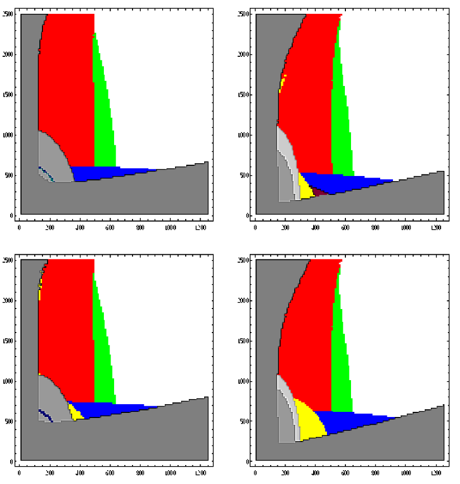
$\tan\beta=55,\,A_{0}=-1\,{\rm TeV},\,{\rm sign}(\mu)>0$                 $\tan\beta=60,\,A_{0}=0,\,{\rm sign}(\mu)>0$

Figure 10: The $(m_{1/2},m_{0})$ mSUGRA plane where SUSY and Higgs particles can be produced at an $e^{+}e^{-}$ collider with a c.m. energy $\sqrt{s}=800$ GeV for different values of $\tan\beta>40$ and $A_{0}$ with sign($\mu)>0$. The notation is as in Fig. 8.

As stated earlier, chargino pair production, $e^{+}e^{-}\to\tilde{\chi}_{1}^{+}\tilde{\chi}_{1}^{-}$, can be probed for mass values up to the kinematical limit, $m_{\tilde{\chi}_{1}^{\pm}}\sim 400$ GeV for $\sqrt{s}=800$ GeV. This implies that for wino–like charginos, i.e. in the region $m_{0}\raisebox{-3.69899pt}{~{}\shortstack{$<$ \\ [-0.07cm] $\sim$}}~{}1.5$ TeV, values $m_{1/2}\sim 1.3m_{\tilde{\chi}_{1}^{\pm}}\sim 500$ GeV can be probed. For larger values of $m_{0}$, the chargino becomes a mixture of higgsino and wino, since $\mu$ is relatively small. This reduces its mass for fixed $m_{1/2}$, so that larger values of $m_{1/2}$ can be probed. As long as the chargino is wino–like, the region where $\tilde{\chi}_{1}^{\pm}$ pair production is accessible is almost independent of $\tan\beta$; however, some parts of this region might be ruled out by the experimental constraints, e.g. for $\tan\beta\sim 5$ [top–left frame in Fig. 9] where a part has been eaten by the $M_{h}\raisebox{-3.69899pt}{~{}\shortstack{$>$ \\ [-0.07cm] $\sim$}}~{}113$ GeV requirement. As noted in the discussion of Fig. 3, choosing $A_{0}=-1$ TeV increases the value of $\mu$ required for EWSB, removing the higgsino and mixed regions, and the maximal value of $m_{1/2}$ that can be probed in chargino pair production becomes independent of $m_{0}$.

Searches for the associated production of the lightest and next–to–lightest neutralinos, $e^{+}e^{-}\to\tilde{\chi}_{1}^{0}\tilde{\chi}_{2}^{0}$, further increase the reach in $m_{1/2}$ in the bino–like limit. In this region the $Z\tilde{\chi}_{1}^{0}\tilde{\chi}_{2}^{0}$ coupling, which is proportional to the product of higgsino components of $\tilde{\chi}_{1}^{0}$ and $\tilde{\chi}_{2}^{0}$, is small. However, selectrons are not too heavy, so selectron exchange in the $t-$channel produces a cross section that should be detectable given the anticipated large luminosity. The situation is thus quite different from the one at LEP2, where the integrated luminosity is three orders of magnitude smaller, in which case the gain from neutralino production over the information obtained from chargino pair production is marginal. However, for very large values of $m_{0}$ and $A_{0}=0$ the lighter neutralinos become almost higgsino–like, and are therefore almost degenerate with the lightest charginos. The reach in chargino and neutralino production then becomes almost the same. Finally, for $A_{0}=-1$ TeV the light neutralinos remain gaugino–like even for $m_{0}\raisebox{-3.69899pt}{~{}\shortstack{$>$ \\ [-0.07cm] $\sim$}}~{}2$ TeV. However, here the selectrons are so heavy that the cross section for neutralino pair production becomes too small even at a high–luminosity collider. In this region of parameter space even the discovery reach could thus still be increased by yet higher luminosities.

Charged sleptons can be produced for relatively small values of $m_{0}$. $\tilde{\tau}_{1}$ pair production remains accessible for values of $m_{0}$ from $\sim 400$ GeV down to the region where the $\tilde{\chi}_{1}^{0}$ is not the LSP. Sneutrinos are heavier than $\tilde{\tau}_{1}$, since they are pure SU(2) doublets. Hence their pair production can be probed in a smaller region of the parameter space. Most slepton pair production channels are insensitive to $\tan\beta$. On the other hand, the region where $\tilde{\tau}_{1}$ pair production, which offers the largest overall reach in the $(m_{1/2},m_{0})$ plane, is accessible becomes smaller (larger) with decreasing (increasing) values of $\tan\beta$. However, much of this changed reach is compensated by the change of the region excluded by the requirement that $\tilde{\chi}_{1}^{0}$ is the LSP.

If $A_{0}$ is small or $\tan\beta$ is large no scalar quarks, not even $\tilde{t}_{1}$ or $\tilde{b}_{1}$ squarks, are light enough to be produced at $\sqrt{s}=800$ GeV, given current experimental constraints. At small $\tan\beta$ the $M_{h}\raisebox{-3.69899pt}{~{}\shortstack{$>$ \\ [-0.07cm] $\sim$}}~{}113$ GeV constraint can only be satisfied if squarks are fairly heavy, whereas at larger $\tan\beta$ the $b\rightarrow s\gamma$ constraint excludes scenarios with light squarks. Only for small $\tan\beta$ and large (and negative) $A_{0}$ does the lightest $\tilde{t}_{1}$ state become accessible in a narrow strip of parameter space with $m_{0}\raisebox{-3.69899pt}{~{}\shortstack{$<$ \\ [-0.07cm] $\sim$}}~{}500$; see the top–left panel in Fig. 9.

For $\tan\beta=40$, Fig. 8, the heavy Higgs bosons $H,A$ and $H^{\pm}$ are accessible only in the small corner $m_{1/2}\sim 250$ GeV, $m_{0}\sim 200$ GeV between the regions ruled out by the $M_{h}$ and the non $\tilde{\chi}_{1}^{0}$ LSP constraints. This region disappears for $\tan\beta\raisebox{-3.69899pt}{~{}\shortstack{$<$ \\ [-0.07cm] $\sim$}}~{}30$ [Fig. 9], but can be significantly extended for larger $\tan\beta$ values [Fig. 10], due to the reduction of $M_{A}$ with increasing $\tan\beta$. On the other hand, choosing $A_{0}=-1$ TeV rather than 0 increases $|\mu|$ as determined from EWSB, and hence also the Higgs boson masses. This explains the absence of a heavy Higgs region in the top–left panel of Fig. 10.

By comparing Figs. 1–3 with Figs. 8–10 we see that the entire 2 $\sigma$ overlap region, where one has at the same time a light Higgs boson with $M_{h}\sim 115$ GeV, a SUSY contribution which accounts for the $(g_{\mu}-2)$ deviation and the requirement of a neutralino being a good Dark Matter candidate, can be covered by neutralino searches already at an 800 GeV collider. Most of this region can also be covered by chargino searches, and much of it can be probed in addition by charged slepton (in particular, $\tilde{\tau}_{1}$) searches; and sneutrinos are accessible in at least part of this region.

$\tan\beta=40\ ,\ A_{0}=0\ ,\ {\rm sign}(\mu)>0$

$m_{0}$

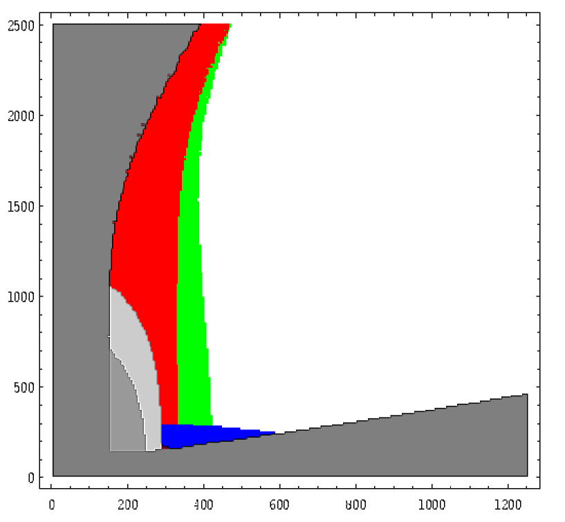
$m_{1/2}$

Figure 11: The $(m_{1/2},m_{0})$ mSUGRA plane where SUSY and Higgs particles can be produced at an $e^{+}e^{-}$ collider with a c.m. energy $\sqrt{s}=500$ GeV. The grey areas are those excluded by theoretical and experimental constraints. The colored regions are those where some cross section is large enough for the particles to be produced: $\tilde{\chi}_{1}^{0}\tilde{\chi}_{2}^{0}$ (green), $\tilde{\chi}_{1}^{+}\tilde{\chi}_{1}^{-}$ (red), $\tilde{\ell}^{+}\tilde{\ell}^{-}$ (blue), $\tilde{\nu}\bar{\tilde{\nu}}$ (purple), $\tilde{t}_{1}\bar{\tilde{t}}_{1}$ (dark blue), $\tilde{b}_{1}\bar{\tilde{b}}_{1}$ (dark blue) and the heavy MSSM $H,A,H^{\pm}$ bosons (yellow). Note that some of these regions are overlapping.

$\tan\beta=5,\,A_{0}=-1\,{\rm TeV},\,{\rm sign}(\mu)>0$               $\tan\beta=10,\,A_{0}=0,\,{\rm sign}(\mu)>0$
$m_{0}$
                                                                                                                                              $m_{1/2}$

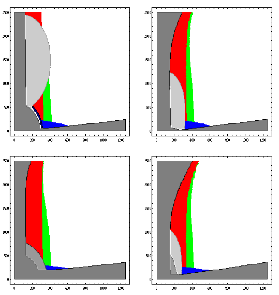
$\tan\beta=20,\,A_{0}=-1\,{\rm TeV},\,{\rm sign}(\mu)>0$               $\tan\beta=30,\,A_{0}=0,\,{\rm sign}(\mu)>0$

Figure 12: The $(m_{1/2},m_{0})$ mSUGRA plane where SUSY and Higgs particles can be produced at an $e^{+}e^{-}$ collider with a c.m. energy $\sqrt{s}=500$ GeV for different values of $\tan\beta<40$ and $A_{0}$ with sign($\mu)>0$. The notation is as in Fig. 11.

$\tan\beta=45,\,A_{0}=-1\,{\rm TeV},\,{\rm sign}(\mu)>0$                 $\tan\beta=50,\,A_{0}=0,\,{\rm sign}(\mu)>0$
$m_{0}$
                                                                                                                                              $m_{1/2}$

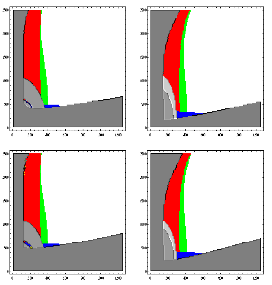
$\tan\beta=55,\,A_{0}=-1\,{\rm TeV},\,{\rm sign}(\mu)>0$                 $\tan\beta=60,\,A_{0}=0,\,{\rm sign}(\mu)>0$

Figure 13: The $(m_{1/2},m_{0})$ mSUGRA plane where SUSY and Higgs particles can be produced at an $e^{+}e^{-}$ collider with a c.m. energy $\sqrt{s}=500$ GeV for different values of $\tan\beta>40$ and $A_{0}$ with sign($\mu)>0$. The notation is as in Fig. 13.

$\tan\beta=40\ ,\ A_{0}=0\ ,\ {\rm sign}(\mu)>0$

$m_{0}$

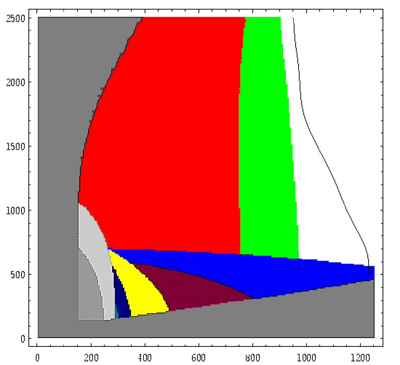
$m_{1/2}$

Figure 14: The $(m_{1/2},m_{0})$ mSUGRA plane where SUSY and Higgs particles can be produced at an $e^{+}e^{-}$ collider with a c.m. energy $\sqrt{s}=1.2$ TeV. The grey areas are those excluded by theoretical and experimental constraints. The colored regions are those where some cross section is large enough for the particles to be produced: $\tilde{\chi}_{1}^{0}\tilde{\chi}_{2}^{0}$ (green), $\tilde{\chi}_{1}^{+}\tilde{\chi}_{1}^{-}$ (red), $\tilde{\ell}^{+}\tilde{\ell}^{-}$ (blue), $\tilde{\nu}\bar{\tilde{\nu}}$ (purple), $\tilde{t}_{1}\bar{\tilde{t}}_{1}$ (dark blue), $\tilde{b}_{1}\bar{\tilde{b}}_{1}$ (dark blue) and the heavy MSSM $H,A,H^{\pm}$ bosons (yellow). Note that some of these regions are overlapping. The black line shows the $5\sigma$ reach contour for sparticles at the LHC in the missing ${\rm E}_{T}$ channel with a luminosity $\int{\cal L}dt=100$ fb^-1; adapted from Ref. [93].

$\tan\beta=5,\,A_{0}=-1\,{\rm TeV},\,{\rm sign}(\mu)>0$                 $\tan\beta=10,\,A_{0}=0,\,{\rm sign}(\mu)>0$
$m_{0}$
                                                                                                                                              $m_{1/2}$

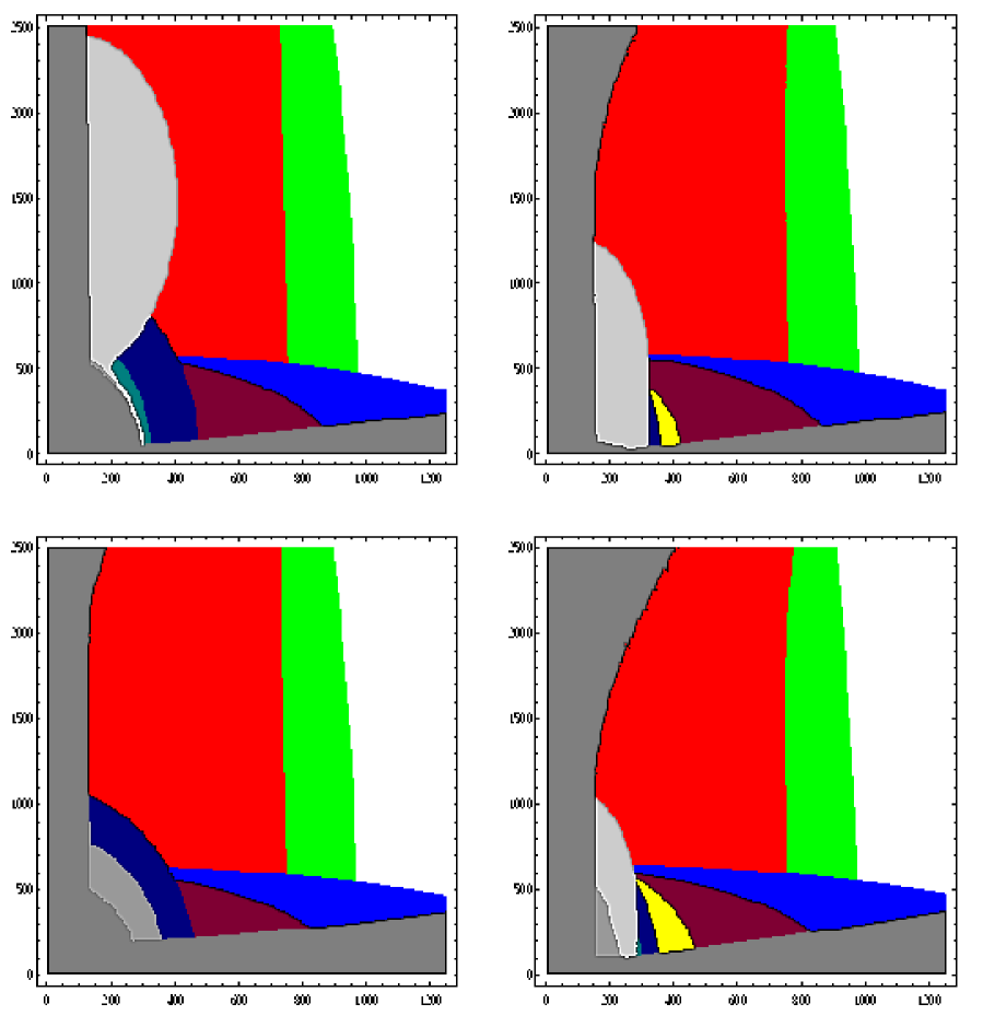
$\tan\beta=20,\,A_{0}=-1\,{\rm TeV},\,{\rm sign}(\mu)>0$                 $\tan\beta=30,\,A_{0}=0,\,{\rm sign}(\mu)>0$

Figure 15: The $(m_{1/2},m_{0})$ mSUGRA plane where SUSY and Higgs particles can be produced at an $e^{+}e^{-}$ collider with a c.m. energy $\sqrt{s}=1.2$ TeV for different values of $\tan\beta<40$ and $A_{0}$ with sign($\mu)>0$. The notation is as in Fig. 14.

$\tan\beta=45,\,A_{0}=-1\,{\rm TeV},\,{\rm sign}(\mu)>0$                 $\tan\beta=50,\,A_{0}=0,\,{\rm sign}(\mu)>0$
$m_{0}$
                                                                                                                                              $m_{1/2}$

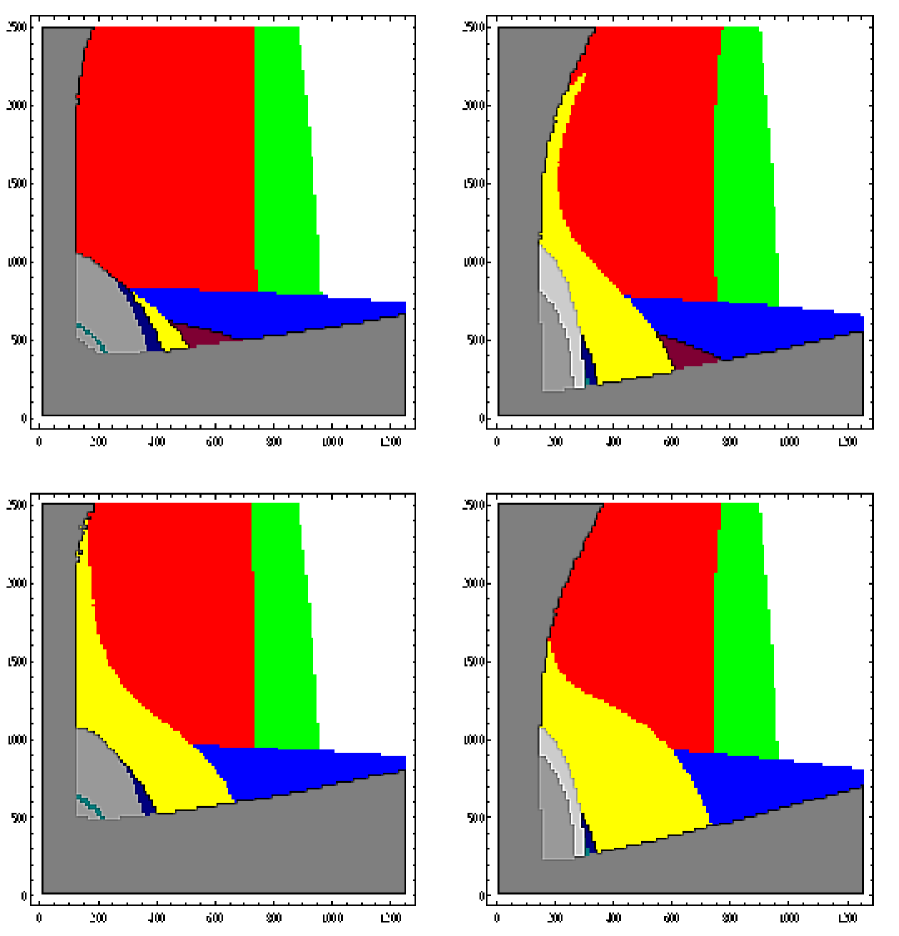
$\tan\beta=55,\,A_{0}=-1\,{\rm TeV},\,{\rm sign}(\mu)>0$                 $\tan\beta=60,\,A_{0}=0,\,{\rm sign}(\mu)>0$

Figure 16: The $(m_{1/2},m_{0})$ mSUGRA plane where SUSY and Higgs particles can be produced at an $e^{+}e^{-}$ collider with a c.m. energy $\sqrt{s}=1.2$ TeV for different values of $\tan\beta>40$ and $A_{0}$ with sign($\mu)>0$. The notation is as in Fig. 14.

Figs. 11–13 show the SUSY reach for $\sqrt{s}=500$ GeV. The regions where charginos, neutralinos and charged $(\tau)$ sleptons are accessible [with the same requirement for cross section and luminosity as before] can essentially be obtained from Figs. 8–10 by simply rescaling $m_{0}$ and $m_{1/2}$. The reach is therefore reduced by a factor $\sim 5/8$ in this case. Of course, the experimental constraints remain the same, and thus exclude a relatively larger region of the parameter space that would have been accessible. For example, for $\tan\beta=5$ and $A_{0}=-1$ TeV [top–left frame in Fig. 12] the $M_{h}\raisebox{-3.69899pt}{~{}\shortstack{$>$ \\ [-0.07cm] $\sim$}}~{}113$ GeV requirement has erased a sizeable region where charginos or neutralinos can be produced at a 500 GeV $e^{+}e^{-}$ collider. In this case, the stop region has also shrunk dramatically. Moreover, sneutrino and heavy Higgs boson production is accessible only in the tiny strip of parameter space at small $m_{0}$ and small $m_{1/2}$ in the bottom–left frame of Fig. 13 where the new contributions to $b\rightarrow s\gamma$ decays are “accidentally” small; see the discussion of Fig. 4.

On the other hand, Figs. 14–16 show that at $\sqrt{s}=1.2$ TeV the prospects for SUSY particle and MSSM Higgs boson production are of course much better. Again by simple rescaling, one reaches values of $m_{1/2}\sim 750$ GeV and 1 TeV from chargino pair production and mixed neutralino pair production, respectively, while $\tilde{\tau}$ pair production can be probed for $m_{0}\raisebox{-3.69899pt}{~{}\shortstack{$<$ \\ [-0.07cm] $\sim$}}~{}700$ GeV. The regions where sneutrinos and top squarks can be produced also increase, and there is now a little corner where even bottom squarks could be accessible [top–left panel in Fig. 15]. For large values of $\tan\beta$, the Higgs domain increases dramatically and for $\tan\beta\raisebox{-3.69899pt}{~{}\shortstack{$>$ \\ [-0.07cm] $\sim$}}~{}55$ [Fig. 16], the heavy $H,A$ and $H^{\pm}$ bosons can be produced in very large areas of the parameter space.

In models with universal soft SUSY breaking gaugino masses the largest value of $m_{1/2}$ which can be probed at a 1.2 TeV $e^{+}e^{-}$ collider through $\mbox{$\tilde{\chi}_{1}^{0}$}\tilde{\chi}_{2}^{0}$ production, $m_{1/2}\simeq 1$ TeV, corresponds to squark and gluino masses in the neighborhood of 2 TeV. This is only slightly lower than the regions which are expected to be probed at the LHC with a high luminosity, where $m_{\tilde{q}}$ and $m_{\tilde{g}}\raisebox{-3.69899pt}{~{}\shortstack{$<$ \\ [-0.07cm] $\sim$}}~{}2.5$ TeV are accessible [93]. This is illustrated in Fig. 14, where we display, together with the reach of an $e^{+}e^{-}$ collider with $\sqrt{s}=1.2$ TeV, the domain that can be probed at the LHC with a luminosity of $\int{\cal L}dt=100$ fb^-1 in the search for squarks and gluinos in the jets plus missing transverse energy channel, shown by the additional line that we adapted from the analysis of Ref. [93]. In addition, there is of course the complementarity between the two colliders: while LHC will primarily probe the strongly interacting particles, the linear collider will be more concerned with the weakly interacting neutralinos, charginos sleptons and Higgs bosons.

5. Conclusions

In this paper, we have performed a comprehensive analysis of all the available constraints on the minimal Supergravity model. We used the state of the art FORTRAN code SuSpect for the calculation of the SUSY and Higgs particle spectrum of the MSSM. We include all presently known important effects [two–loop renormalization equations for couplings and gaugino masses, the complete one–loop effective potential for electroweak symmetry breaking, and the radiative corrections to standard fermion, Higgs boson and sparticle masses]. This allowed us to fairly reliably delineate the regions of the mSUGRA parameter space which are still allowed by theoretical constraints [from a proper EWSB breaking, neutralino LSP, non–tachyonic Higgs and SUSY particles, etc..] and by the present experimental data [i.e., the bounds on SUSY particle and Higgs boson masses from negative searches at LEP2 and the Tevatron, the measurement of the $b\to s\gamma$ branching ratio, and the precision electroweak measurements]. We have also indicated the regions of parameter space where one obtains a light Higgs boson with a mass $M_{h}\sim 115$ GeV, where the SUSY contributions can account for the deviation of the experimental value of $(g_{\mu}-2)$ from its Standard Model prediction, and where the lightest neutralino makes a good Dark Matter candidate.

When taken at face value, our calculation shows that all constraints [including the positive indications] can be satisfied only in fairly narrow regions of mSUGRA parameter space. However, experimental errors on the input parameters [in particular, on the mass of the top quark; Fig. 5], as well as theoretical uncertainties, are still significant. The latter lead to a residual scale dependence of our results [Fig. 6], as well as to a significant uncertainty in the prediction of the mass of the lightest Higgs boson. We also repeat our cautionary remarks regarding the interpretation of the $b\rightarrow s\gamma$ and, in particular, the Dark Matter constraints, which can be circumvented without significantly altering any collider signal, at the cost of a somewhat more contrived model of particle physics and/or cosmology. With these caveats in mind, the main outcome of our analysis can be summarized as follows:

– There are large areas of the $(m_{1/2},m_{0})$ parameter space which are still allowed by present experimental constraints. In particular, for large enough values of $\tan\beta$, the bound on the lightest $h$ boson mass, $M_{h}\raisebox{-3.69899pt}{~{}\shortstack{$>$ \\ [-0.07cm] $\sim$}}~{}113$ GeV, does not place too severe constraints. If $\mu>0$, which is favored by the $(g_{\mu}-2)$ anomaly, the constraint from the radiative decay $b\to s\gamma$ is not too restrictive [in our conservative interpretation of experimental and theoretical errors] even for large values of $\tan\beta$. In fact, if $A_{0}=0$ it is always superseded by the Higgs boson mass constraint, but for $A_{0}=-1$ TeV the $b\rightarrow s\gamma$ constraint can be more severe [Figs. 3 and 4]. Precision electroweak measurements are easily accommodated in the mSUGRA framework.

– For $\tan\beta\raisebox{-3.69899pt}{~{}\shortstack{$>$ \\ [-0.07cm] $\sim$}}~{}10$ and small values of the trilinear coupling $A_{0}$, the requirement of a Higgs boson in the mass range 113 GeV $\raisebox{-3.69899pt}{~{}\shortstack{$<$ \\ [-0.07cm] $\sim$}}~{}M_{h}\raisebox{-3.69899pt}{~{}\shortstack{$<$ \\ [-0.07cm] $\sim$}}~{}117$ GeV favors moderate values of the common gaugino mass parameter, $m_{1/2}\raisebox{-3.69899pt}{~{}\shortstack{$<$ \\ [-0.07cm] $\sim$}}~{}500$ GeV, leading to relatively light chargino and neutralino states, $m_{\tilde{\chi}_{1}^{\pm}}\sim m_{\tilde{\chi}_{2}^{0}}\sim 2m_{\tilde{\chi}_{1}^{0}}\raisebox{-3.69899pt}{~{}\shortstack{$<$ \\ [-0.07cm] $\sim$}}~{}400$ GeV. For large (and negative) values of $A_{0}$, which lead to a strong mixing in the stop sector, a Higgs mass in this range can be accommodated in large regions of the parameter space even for rather small $\tan\beta(\sim 5)$ values. In this case $\tilde{t}_{1}$ squarks can be rather light, if the soft breaking parameters $m_{0}$ and $m_{1/2}$ are not too high. The range of $m_{1/2}$ favored by the LEP Higgs evidence strongly depends on the exact value of $M_{t}$. We thus eagerly anticipate improved measurements of this important parameter at the current run of the Tevatron collider.

– The $(g_{\mu}-2)$ excess, which can be accommodated in the MSSM only if $\mu>0$, typically gives a stronger upper bound on $m_{0}$ than the requirement $M_{H}=115\pm 2$ GeV. For $\tan\beta\sim 40$, $m_{0}$ and $m_{1/2}$ values below $\sim 600$ GeV [and slightly above $\sim 300$ GeV] are needed if the experimental value is to be reproduced within $1\sigma$, implying again relatively light electroweak gaugino and slepton states. However, the value of this upper bound increases roughly proportional to $\tan\beta$, so that at $\tan\beta=60$, $m_{0}$ as large as 1.0 (1.6) TeV can be accommodated at the 1 (2) $\sigma$ level.

– For small and moderate $\tan\beta(\raisebox{-3.69899pt}{~{}\shortstack{$<$ \\ [-0.07cm] $\sim$}}~{}40)$ the requirement that the density of the lightest neutralinos left over from the Big Bang is in the right range to account for the Dark Matter density in the Universe is very constraining indeed. In this case most of the region where $\Omega_{\tilde{\chi}_{1}^{0}}h^{2}$ is “naturally” in the interesting range is excluded by the Higgs mass constraints, which requires SUSY breaking masses above those preferred by Dark Matter calculations. Only a small band in the region with a relatively light bino–like neutralino and relatively light sleptons survives. In addition, there are “exceptional” regions: a narrow strip in the $\tilde{\tau}_{1}\mbox{$\tilde{\chi}_{1}^{0}$}$ co–annihilation region near the boundary where the $\tilde{\tau}_{1}$ slepton is the LSP, and a strip in the focus point region at large $m_{0}$ and small $m_{1/2}$ values where neutralinos and charginos are relatively light and have large higgsino components. Requiring in addition $M_{h}=115\pm 2$ GeV and a SUSY interpretation for the $(g_{\mu}-2)$ anomaly removes most of these “exceptional” regions with acceptable relic density. On the other hand, for large values of $\tan\beta(\raisebox{-3.69899pt}{~{}\shortstack{$>$ \\ [-0.07cm] $\sim$}}~{}50)$, the area of the $(m_{0},m_{1/2})$ parameter space favored by cosmology extends significantly due to the opening of the pseudoscalar $A$–boson pole. This allows to fit all the requirements [$M_{h}$, $(g_{\mu}-2)$ and the DM constraint] in a somewhat larger area of the $(m_{0},m_{1/2})$ parameter space. However, the Higgs mixing parameter $\overline{m}_{3}^{2}$ in the scalar potential needs to be fine-tuned quite severely to accommodate very large values of $\tan\beta$ [94].

– In spite of the strong constraints on the mSUGRA parameter space obtained by taking seriously all the positive indications for supersymmetry it is still not possible to give tight limits on any one single parameter. We found overlap regions with $5\leq\tan\beta\leq 60$, 0.1 TeV $\raisebox{-3.69899pt}{~{}\shortstack{$<$ \\ [-0.07cm] $\sim$}}~{}m_{0}\raisebox{-3.69899pt}{~{}\shortstack{$<$ \\ [-0.07cm] $\sim$}}~{}$ 1.5 TeV, 160 GeV $\raisebox{-3.69899pt}{~{}\shortstack{$<$ \\ [-0.07cm] $\sim$}}~{}m_{1/2}\raisebox{-3.69899pt}{~{}\shortstack{$<$ \\ [-0.07cm] $\sim$}}~{}$ 550 GeV and for both $A_{0}=0$ and $A_{0}=-1$ TeV. Allowing for a large negative $A_{0}$ plays an important role in extending the allowed region to smaller values of $\tan\beta$. On the other hand, for larger $\tan\beta$, $A_{0}=0$ is generally preferred, mostly due to the $b\rightarrow s\gamma$ constraint. This implies that the allowed region in the $(m_{1/2},m_{0})$ plane could be further extended by considering more choices for $A_{0}$, including positive values.

We have then analyzed the prospects for producing SUSY particles and heavy Higgs bosons at high–energy and high–luminosity $e^{+}e^{-}$ colliders, requiring a sample of 50 events per year to establish discovery; this should be sufficient in the clean environment provided by $e^{+}e^{-}$ colliders. At c.m. energy $\sqrt{s}\sim 800$ GeV, we have shown that charginos, neutralinos and sleptons [in particular $\tilde{\tau}$ sleptons and sneutrinos] are accessible in rather large regions of the parameter space. In particular, already at $\sqrt{s}=800$ GeV associated $\mbox{$\tilde{\chi}_{1}^{0}$}\tilde{\chi}_{2}^{0}$ production is accessible in the entire overlap region described above. Almost all of this region can also be probed through $\tilde{\chi}_{1}^{\pm}$ pair production, and in much of this region $\tilde{\tau}_{1}$ pair production can also be studied. In some areas of the parameter space, top squarks and even bottom squarks can be produced. In the large $\tan\beta$ regime, where the present indications for SUSY can be accommodated in a larger fraction of the $(m_{1/2},m_{0})$ plane, there is a large region of parameter space where the heavier MSSM Higgs bosons $H,A$ and $H^{\pm}$ are kinematically accessible.

Even for lower c.m. energies, $\sqrt{s}\sim 500$ GeV, charginos, neutralinos and charged $(\tilde{\tau})$ sleptons can be produced in a significant region of parameter space not excluded by the present constraints. However, discovery of sparticles can then no longer be guaranteed [in the framework of mSUGRA] even if all positive indications for SUSY hold up to further scrutiny. On the other hand, if the c.m. energy of the collider is increased to $\sqrt{s}=1.2$ TeV, the mSUGRA parameter space where SUSY and Higgs particles are kinematically accessible and have sufficiently large cross sections to be detected becomes very wide. The $e^{+}e^{-}$ collider will then have a search potential of SUSY particles that is comparable to the range probed at the LHC. This is largely due to the fact that, thanks to the high luminosities expected at future $e^{+}e^{-}$ colliders, the process $e^{+}e^{-}\to\tilde{\chi}_{1}^{0}\tilde{\chi}_{2}^{0}$ can probe large values of the parameter $m_{1/2}$: only from kinematical arguments, values $m_{1/2}\sim 1$ TeV can be probed at $\sqrt{s}=1.2$ TeV, corresponding to a gluino mass of the order of 2 TeV. Heavy Higgs particles can be searched if their masses are smaller than the beam energy. For large values of $\tan\beta$, this occurs in a large region of the mSUGRA parameter space.

One might naively argue that the LHC would still have an edge over a 1.2 TeV $e^{+}e^{-}$ collider, since at the LHC the heaviest sparticles (squarks and gluinos) are produced directly, allowing access to lighter sparticles (neutralinos, charginos and sleptons) through cascade decays. In contrast, if $m_{1/2}$ is indeed near 1 TeV [which seems highly unlikely, given the original motivation for “weak–scale” SUSY], an $e^{+}e^{-}$ collider would “only” have access to one or two production channels. However, in such a pessimistic scenario the relatively small production cross section and the large number of possible decay modes will make it very difficult, if not impossible, to study any one decay mode in detail at the LHC. So far at least the ability of LHC experiments to perform such studies has only been demonstrated [23] for significantly lower mass scales, i.e. much higher production cross sections.

On the other hand, precision measurements at an $e^{+}e^{-}$ collider could reveal a great deal about the MSSM spectrum even if only the “lower end” of the sparticle spectrum is accessible [91]. In particular, thanks to the precise knowledge of the initial $e^{+}$ and $e^{-}$ beam energies, threshold scans allow the measurement of some sparticle masses at the permille level. Making use of the ability to vary the beam polarization at will, various couplings appearing in the production cross sections of SUSY and Higgs particles can be measured with a high precision. Additional couplings can be determined through the careful measurement of decay branching ratios.

The amount of information on the SUSY model can be maximized by combining results from a high–luminosity $e^{+}e^{-}$ collider with those obtained at the LHC and elsewhere. In the near future measurements at relatively low energies [at the $B-$factories, from searches for $\mu\rightarrow e\gamma$ decays etc.] will yield new information on the flavor structure of the soft breaking terms. Any positive signal for large flavor violation would rule out the mSUGRA model as commonly defined, while absence of such a signal would strengthen the motivation for assuming universal sparticle masses at some high scale. Of course, the crucial test of SUSY will have to come from high–energy colliders. A combination of the information on sleptons and electroweak gauginos that one can obtain at $e^{+}e^{-}$ colliders with the information on squark and gluino production obtained at the LHC would allow very stringent tests of the model. The flavor–conserving parts of the SUSY Lagrangian at the low energy scale can then be reconstructed to a considerable extent. Under the assumption of a Grand Desert, the underlying structure of the theory at the GUT or Planck scale can then be studied. For instance the combination of, on the one hand, the measurement of the electroweak gaugino [chargino and neutralino] masses at the linear collider with the measurement of the gluino mass at the LHC allows to test gaugino mass unification. Similarly, the measurement of the slepton and Higgs boson masses at an $e^{+}e^{-}$ collider together with the squark mass determination at the LHC would allow to verify the second mSUGRA assumption that scalar soft SUSY breaking mass parameters are also unified at the GUT scale [96]. A high–energy, high–luminosity $e^{+}e^{-}$ linear collider would thus be crucial for fully testing the mSUGRA model.

Of course it is quite possible, perhaps even likely, that mSUGRA in its simplest version will already have been excluded before the next $e^{+}e^{-}$ linear collider commences operation. However, most of our conclusions remain valid in a more general supersymmetric context. In particular, the SUSY mass scales indicated by the positive evidence for a 115 GeV Higgs boson and for a SUSY loop contribution to $(g_{\mu}-2)$ are not very sensitive to details of the SUSY model. Our conclusions will then remain qualitatively the same, as long as there are no large hierarchies between soft breaking parameters that are assumed to be unified in mSUGRA [i.e. as long as all gaugino masses and all scalar masses are similar at some high scale; a very large or very small ratio of these two masses can be accommodated even in mSUGRA]. In the absence of a compelling model of supersymmetry breaking it becomes absolutely essential to collect as many independent pieces of information about the soft breaking terms as possible. By studying a highly constrained model we have thus chosen a scenario which minimizes the advantages of $e^{+}e^{-}$ colliders. As argued above, even in this context the prospects for SUSY studies at such colliders seem very bright. We are thus confident that linear high energy, high luminosity $e^{+}e^{-}$ colliders will play a crucial role in revealing the secrets of Supersymmetry breaking, assuming that Nature indeed makes use of the beautiful idea of weak scale Supersymmetry.

Acknowledgments:

We thank Ben Allanach, Asesh Datta, Paolo Gambino, Jean–Francois Grivaz, Gilbert Moultaka and Margarete Mühlleitner for discussions. Special thanks go to Francois Richard and Peter Zerwas for their interest in this work and for helpful suggestions. This work is supported in part by the Euro–GDR Supersymétrie and by the European Union under contract HPRN-CT-2000-00149. The work of M.D. is supported in part by the “Sonderforschungsbereich 375–95 für Astro–Teilchenphysik” der Deutschen Forschungsgemeinschaft.

Appendix: Production cross sections

In this Appendix, we present for completeness expressions for the production cross sections in $e^{+}e^{-}$ collisions for diagonal and mixed pairs of charginos [97], neutralinos [98], sleptons [99] and squarks [86] as well as for the heavy MSSM Higgs bosons [100, 89], using a unified notation.

1. Neutralino and Chargino production

The integrated cross section for mixed neutralino $\tilde{\chi}_{i}^{0}\tilde{\chi}_{j}^{0}$ pair production can be written as

$$\sigma(e^{+}e^{-}\to\tilde{\chi}^{0}_{i}\tilde{\chi}_{j}^{0}) = \frac{1}{1+\delta_{ij}}\frac{2\pi\alpha^{2}}{s_{W}^{4}c_{W}^{4}}\,\frac{\lambda^{1/2}_{ij}}{s}(\sigma_{ZZ}+\sigma_{\tilde{e}\tilde{e}}+\sigma_{Z\tilde{e}}),$$ (A.1)

with $\lambda^{1/2}_{ij}$ being the usual phase–space function with the reduced masses:

$$\lambda^{1/2}_{ij}=\frac{1}{2}\bigg{[}(1-\mu_{i}^{2}-\mu_{j}^{2})^{2}-4\mu_{i}^{4}\mu_{j}^{4}\bigg{]}^{1/2}\ \ {\rm with}\ \mu_{i}^{2}=m_{\tilde{\chi}_{i}^{0}}^{2}/s\ ,\ \mu_{j}^{2}=m_{\tilde{\chi}_{j}^{0}}^{2}/s.$$ (A.2)

The contribution of the $s$–channel $Z$–boson exchange, the $t$–channel $\tilde{e}$ exchange and the $Z\tilde{e}$ interference are expressed in terms of $\lambda_{ij}$ and the final particle energies, $e_{i,j}=\sqrt{\lambda_{ij}+\mu^{2}_{i,j}}$ [note that the neutralino masses here are the eigenvalues and the sign must be included]:

$$\sigma_{ZZ} = \frac{(O^{{}^{\prime\prime}L}_{ji})^{2}(L_{e}^{2}+R_{e}^{2})s^{2}}{|D_{Z}(s)|^{2}}\Bigg{[}\frac{2}{3}\lambda_{ij}+2e_{i}e_{j}-2\mu_{i}\mu_{j}\Bigg{]},$$

$$\sigma_{Z\tilde{e}} = \frac{c_{W}^{2}O^{{}^{\prime\prime}L}_{ji}s}{{\cal R}eD_{Z}(s)}\Bigg{[}L_{e}f_{e_{i}}^{L}f_{e_{j}}^{L}[I_{1}(\mu^{2}_{\tilde{e}_{L}})-\mu_{i}\mu_{j}{\rm L}(\mu^{2}_{\tilde{e}_{L}})]-R_{e}f_{e_{i}}^{R}f_{e_{j}}^{R}[I_{1}(\mu^{2}_{\tilde{e}_{R}})-\mu_{i}\mu_{j}{\rm L}(\mu^{2}_{\tilde{e}_{R}})]\Bigg{]},$$

$$\sigma_{\tilde{e}\tilde{e}} = \frac{c_{W}^{4}}{4}\Bigg{[}(f_{e_{i}}^{L}f_{e_{j}}^{L})^{2}[I_{2}(\mu^{2}_{\tilde{e}_{L}})-\mu_{i}\mu_{j}I_{3}(\mu^{2}_{\tilde{e}_{L}})]-(f_{e_{i}}^{R}f_{e_{j}}^{R})^{2}[I_{2}(\mu^{2}_{\tilde{e}_{R}})-\mu_{i}\mu_{j}I_{3}(\mu^{2}_{\tilde{e}_{R}})],\Bigg{]}$$ (A.3)

with $D_{Z}(s)=s-M_{Z}^{2}+i\Gamma_{Z}M_{Z}$. The various couplings are given, in terms of the weak isospin and electric charge of the electron and the elements of the matrix $Z$ which diagonalizes the neutralino mass matrix [which can be found in Ref. [67] for instance] by:

$$L_{e}=I_{3L}^{e}-Q_{e}s_{W}^{2}\ \ ,\ \ R_{e}=-Q_{e}s_{W}^{2}\ \ ,\ \ O^{{}^{\prime\prime}L}_{ij}=-\frac{1}{2}Z_{i3}Z_{j3}+\frac{1}{2}Z_{i4}Z_{j4},$$

$$f_{e_{i}}^{L}=\sqrt{2}[(I_{3L}^{e}-Q_{e})\tan\theta_{W}Z_{i1}-I_{3L}^{e}Z_{i2}]\ \ ,\ \ f_{e_{i}}^{R}=\sqrt{2}Q_{e}\tan\theta_{W}Z_{i1}.$$ (A.4)

The kinematical functions $I_{1},I_{2}$ and $I_{3}$, with $\mu^{2}_{\tilde{e}_{k}}=m_{\tilde{e}_{k}}^{2}/s$ and $k=L,R$, read:

$$I_{1}(\mu) = \bigg{[}(\mu_{i}^{2}+\mu_{j}^{2}-2\mu^{2})^{2}-(e_{i}-e_{j})^{2}\bigg{]}\frac{{\rm L}(\mu^{2})}{4\lambda_{ij}^{1/2}}-\bigg{[}\mu_{i}^{2}+\mu_{j}^{2}-2\mu^{2}+1\bigg{]},$$

$$I_{2}(\mu) = \frac{(\mu^{2}_{i}+\mu^{2}_{j}-2\mu^{2})(\mu_{i}^{2}+\mu_{j}^{2}-2\mu^{2}-1)-2(\lambda_{ij}-e_{i}e_{j})}{\frac{1}{4}(\mu_{i}^{2}+\mu_{j}^{2}-2\mu^{2}-1)-\lambda_{ij}}-(\mu_{i}^{2}+\mu_{j}^{2}-2\mu^{2})\frac{{\rm L}(\mu^{2})}{4\lambda_{ij}^{1/2}},$$

$$I_{3}(\mu) = \frac{{\rm L}(\mu^{2})}{4\lambda_{ij}^{1/2}(\mu_{i}^{2}+\mu_{j}^{2}-2\mu^{2}-1)},$$ (A.5)

and

$${\rm L}(\mu^{2})=\log\,\frac{\mu_{i}^{2}+\mu_{j}^{2}-2\mu^{2}-1+2\lambda^{1/2}_{ij}}{\mu_{i}^{2}+\mu_{j}^{2}-2\mu^{2}-1-2\lambda^{1/2}_{ij}}.$$ (A.6)

For chargino pair production, the cross section can be decomposed into the $s$–channel $\gamma,Z$–exchange contributions, the $t$–channel $\tilde{\nu}_{e}$ contribution and the interference terms:

$$\sigma(e^{+}e^{-}\to\tilde{\chi}^{+}_{i}\tilde{\chi}_{j}^{-}) = 8\pi\alpha^{2}\frac{\lambda^{1/2}_{ij}}{s}(\sigma_{s}+\sigma_{t}+\sigma_{st}).$$ (A.7)

Using the same notation as previously [but now $\mu_{i}^{2}=m_{\tilde{\chi}_{i}^{\pm}}^{2}/s$ and $\mu_{j}^{2}=m_{\tilde{\chi}_{j}^{\pm}}^{2}/s$] one has for the different components:

$$\sigma_{s} = \delta_{ij}\left[1+\frac{1}{2c_{W}^{2}c_{W}^{2}}\frac{s}{{\cal R}eD_{Z}(s)}(L_{e}+R_{e})(O^{{}^{\prime}L}_{ij}+O^{{}^{\prime}R}_{ij})\right]\left(\frac{1}{3}\lambda_{ij}+e_{i}e_{j}+\mu_{i}\mu_{j}\right)$$

$$+\frac{1}{4s_{W}^{4}c_{W}^{4}}\frac{s^{2}}{|D_{Z}(s)|^{2}}(L_{e}^{2}+R_{e}^{2})\bigg{[}\bigg{(}(O^{{}^{\prime}L}_{ij})^{2}+(O^{{}^{\prime}R}_{ij})^{2}\bigg{)}\left(\frac{1}{3}\lambda_{ij}+e_{i}e_{j}\right)+2O^{{}^{\prime}L}_{ij}O^{{}^{\prime}R}_{ij}\mu_{i}\mu_{j}\bigg{]},$$

$$\sigma_{st} = -\frac{V_{i1}V_{j1}}{8s_{W}^{2}}\bigg{\{}\delta_{ij}\bigg{[}I_{1}(\mu^{2}_{\tilde{\nu}})-\mu_{i}\mu_{j}{\rm L}(\mu^{2}_{\tilde{\nu}})\bigg{]}+\frac{1}{s_{W}^{2}c_{W}^{2}}\frac{s}{{\cal R}eD_{Z}(s)}L_{e}\bigg{[}O^{{}^{\prime}L}_{ij}I_{1}(\mu^{2}_{\tilde{\nu}})-O^{{}^{\prime}R}_{ij}\mu_{i}\mu_{j}{\rm L}(\mu^{2}_{\tilde{\nu}})\bigg{]}\bigg{\}},$$

$$\sigma_{t} = \frac{|V_{i1}|^{2}|V_{j1}|^{2}}{16s_{W}^{4}}\bigg{[}I_{2}(\mu^{2}_{\tilde{\nu}})-\mu_{i}\mu_{j}I_{3}(\mu^{2}_{\tilde{\nu}})\bigg{]},$$ (A.8)

with the additional couplings $O^{{}^{\prime}L}_{ij},O^{{}^{\prime}R}_{ij}$ expressed in terms of the elements of the matrices $U$ and $V$ which diagonalize the chargino mass matrix

$$O^{{}^{\prime}L}_{ij}=\delta_{ij}s_{W}^{2}-V_{i1}V_{j1}-\frac{1}{2}V_{i2}V_{j2}\ ,\ O^{{}^{\prime}R}_{ij}=\delta_{ij}s_{W}^{2}-U_{i1}U_{j1}-\frac{1}{2}U_{i2}U_{j2}.$$ (A.9)

2. Selectron and Sneutrino production

The integrated cross section for the pair production of left–handed or right–handed selectrons, which occurs through the $s$–channel $\gamma$ and $Z$ boson exchanges and the $t$–channel exchange of the four neutralinos $\tilde{\chi}_{l}^{0}$, can be written as

$$\sigma(e^{+}e^{-}\to\tilde{e}_{i}\tilde{e}_{i}^{*}) = \frac{\pi\alpha^{2}}{s}\Bigg{\{}\frac{1}{3}\beta^{3}_{i}\Bigg{[}Q_{e}^{2}Q_{\tilde{e}}^{2}+\frac{Q_{e}Q_{\tilde{e}}}{s_{W}^{2}c_{W}^{2}}\tilde{a}_{i}L_{e}\frac{s}{{\cal R}eD_{Z}(s)}+\frac{L_{e}^{2}+R_{e}^{2}}{2c_{W}^{4}s_{W}^{4}}\tilde{a}_{i}^{2}\frac{s^{2}}{|D_{Z}(s)|^{2}}\Bigg{]}$$ (A.10)

$$+4\sum_{l=1}^{4}\sum_{k=1}^{4}|\lambda_{il}|^{2}|\lambda_{ik}|^{2}H_{ilk}+2\sum_{l=1}^{4}|\lambda_{il}|^{2}\bigg{[}Q_{e}Q_{\tilde{e}}+\frac{\tilde{a}_{i}L_{e}}{c_{W}^{2}s_{W}^{2}}\bigg{]}F_{il}\Bigg{\}}.$$

The notation is as before with $\beta_{i}$ is the selectron velocity $\beta_{i}^{2}=1-4\mu_{i}^{2}$ where in this case $\mu_{i}^{2}=m_{\tilde{e}_{i}}^{2}/s$. The couplings $\tilde{a}_{i}$ of the selectrons to the $Z$ boson and the couplings $\lambda_{ik}$ between the electron, the selectrons $\tilde{e}_{i}$ and the neutralinos $\tilde{\chi}_{k}^{0}$ are given by

$$\tilde{a}_{L}=I_{3L}^{\tilde{e}}-Q_{\tilde{e}}s_{W}^{2}\ \ \ ,\ \ \ \tilde{a}_{R}=-Q_{\tilde{e}}s_{W}^{2},\hskip 85.35826pt$$

$$\lambda_{Lk}=\frac{1}{2}\left(Z^{\prime}_{k1}-\frac{\tilde{a}_{L}}{c_{W}s_{W}}Z^{\prime}_{k2}\right)\ \ ,\ \ \lambda_{Rk}=-\frac{1}{2}\left(Z^{\prime}_{k1}-\frac{\tilde{a}_{R}}{c_{W}s_{W}}Z^{\prime}_{k2}\right),$$ (A.11)

with the rotated matrix elements: $Z^{\prime}_{k1}=Z_{k1}c_{W}+Z_{k2}s_{W}$ and $Z^{\prime}_{k2}=-Z_{k1}s_{W}+Z_{k2}c_{W}$. The kinematical functions $F$ and $H$, in the case where the two exchanged neutralinos $\tilde{\chi}_{l}^{0}$ and $\tilde{\chi}_{k}^{0}$ are different, is given by

$$H_{ilk}=+\frac{1}{2}\frac{F_{il}-F_{ik}}{\mu_{l}^{2}-\mu_{k}^{2}},$$ (A.12)

where $\mu_{l}^{2}=m_{\tilde{\chi}_{l}^{0}}^{2}/s,\mu_{k}^{2}=m_{\tilde{\chi}_{k}^{0}}^{2}/s$ and the function $F_{ik}$ reads:

$$F_{ik}=\beta_{i}(-1+2\mu_{i}^{2}-2\mu_{k}^{2})+2[\mu_{k}^{2}+(\mu_{i}^{2}-\mu_{k}^{2})^{2}]\,\log\frac{2\mu_{i}^{2}-2\mu_{k}^{2}-(1+\beta_{i})}{2\mu_{i}^{2}-2\mu_{k}^{2}-(1-\beta_{i})}.$$ (A.13)

In the case where the exchanged neutralinos are the same [i.e for the squared amplitudes], the function $H_{ilk}$ with $l=k$ reduces to:

$$H_{ikk}=-2\beta_{i}+(1-2\mu_{i}^{2}+2\mu_{k}^{2})\,\log\frac{2\mu_{i}^{2}-2\mu_{k}^{2}-(1+\beta_{i})}{2\mu_{i}^{2}-2\mu_{k}^{2}-(1-\beta_{i})}.$$ (A.14)

For the production of selectrons of different types, there is no $s$–channel gauge boson exchange and the cross section simply reads:

$$\sigma(e^{+}e^{-}\to\tilde{e}_{L}\tilde{e}_{R}^{*}) = \frac{4\pi\alpha^{2}}{s}\sum_{l=1}^{4}\sum_{k=1}^{4}\lambda_{Ll}\lambda_{Rl}\lambda_{Lk}\lambda_{Rk}H_{lk},$$ (A.15)

where in terms of the phase space function defined in eq. (A.2),

$$l\neq k\ :\ \ H_{lk} = -\frac{\mu_{l}\mu_{k}}{\mu_{l}^{2}-\mu_{k}^{2}}\bigg{[}\log\frac{\mu_{\tilde{e}_{L}}^{2}+\mu_{\tilde{e}_{R}}^{2}-2\mu_{l}^{2}-1-\lambda_{\tilde{e}_{L}\tilde{e}_{R}}^{1/2}}{\mu_{\tilde{e}_{L}}^{2}+\mu_{\tilde{e}_{R}}^{2}-2\mu_{l}^{2}-1+\lambda_{\tilde{e}_{L}\tilde{e}_{R}}^{1/2}}-(l\leftrightarrow k)\,\Bigg{]},$$

$$l=k\ :\ \ H_{kk} = \frac{4\lambda_{\tilde{e}_{L}\tilde{e}_{R}}^{1/2}\mu_{l}^{2}}{(\mu_{\tilde{e}_{L}}^{2}+\mu_{\tilde{e}_{R}}^{2}-2\mu_{l}^{2}-1-\lambda_{\tilde{e}_{L}\tilde{e}_{R}}^{1/2})(\mu_{\tilde{e}_{L}}^{2}+\mu_{\tilde{e}_{R}}^{2}-2\mu_{l}^{2}-1+\lambda_{\tilde{e}_{L}\tilde{e}_{R}}^{1/2})}.$$ (A.16)

For the pair production of the electron sneutrino, the expression of the total cross section is similar to the one of left–handed selectrons except that the $s$–channel photon exchange is absent and the couplings are different. It is given by:

$$\sigma(e^{+}e^{-}\to\tilde{\nu}_{e}\tilde{\nu}_{e}^{*}) = \frac{\pi\alpha^{2}}{s}\Bigg{\{}\frac{1}{3}\beta^{3}_{\tilde{\nu}}\frac{L_{e}^{2}+R_{e}^{2}}{2c_{W}^{4}s_{W}^{4}}\tilde{a}_{\nu}^{2}\frac{s^{2}}{|D_{Z}(s)|^{2}}\Bigg{]}$$ (A.17)

$$+4\sum_{l=1}^{4}\sum_{k=1}^{4}|\lambda_{\tilde{\nu}l}|^{2}|\lambda_{\tilde{\nu}k}|^{2}H_{\tilde{\nu}lk}+\frac{2\tilde{a}_{\nu}^{2}}{s_{W}^{2}c_{W}^{2}}\sum_{l=1}^{4}|\lambda_{\tilde{\nu}l}|^{2}\bigg{]}F_{\tilde{\nu}l}\Bigg{\}},$$

where the functions $H$ and $F$ are given by the previous equations with $\mu_{i}$ replaced by $\mu_{\tilde{\nu}_{e}}$ and

$$\tilde{a}_{\nu}=\frac{1}{2}\ \ ,\ \ \lambda_{\tilde{\nu}l}=\frac{1}{2s_{W}}V_{1l}.$$ (A.18)

3. Sfermion pair production

For sleptons of the second and third generation and for squarks, there is only $s$ channel gauge boson exchange and the production cross sections, in the absence of sfermion mixing, is simply given by:

$$\sigma(e^{+}e^{-}\to\tilde{f}_{i}\tilde{f}_{i}^{*})=\frac{\pi\alpha^{2}N_{c}}{3s}\beta_{i}^{3}\Bigg{[}Q_{e}^{2}Q_{\tilde{f}}^{2}+\frac{Q_{e}Q_{\tilde{f}}}{s_{W}^{2}c_{W}^{2}}\tilde{a}_{i}L_{e}\frac{s}{{\cal R}eD_{Z}(s)}+\frac{L_{e}^{2}+R_{e}^{2}}{2c_{W}^{4}s_{W}^{4}}\tilde{a}_{i}^{2}\frac{s^{2}}{|D_{Z}(s)|^{2}}\Bigg{]},$$ (A.19)

with $N_{c}$ the color factor, $N_{c}=3(1)$ for squarks (sleptons), and the $\tilde{a}_{i}$ are as in eq. (A.11) for a given charge and isospin. However, in the case of third generation sfermions, the mixing between the left–handed and right–handed states has to be included. In this case the cross section becomes slightly more involved and can be written as:

$$\sigma(e^{+}e^{-}\to\tilde{f}_{i}\tilde{f}_{j}^{*})=\frac{\pi\alpha^{2}N_{c}}{3s}\lambda_{ij}^{3/2}\Bigg{[}\delta_{ij}\bigg{(}Q_{e}^{2}Q_{\tilde{f}}^{2}+\frac{Q_{e}Q_{\tilde{f}}}{s_{W}^{2}c_{W}^{2}}\frac{s\tilde{a}_{ij}L_{e}}{{\cal R}eD_{Z}(s)}\bigg{)}+\frac{L_{e}^{2}+R_{e}^{2}}{2c_{W}^{4}s_{W}^{4}}\frac{\tilde{a}_{ij}^{2}s^{2}}{|D_{Z}(s)|^{2}}\Bigg{]},$$ (A.20)

with $\lambda_{ij}$ the phase space function eq. (A.2) and the couplings $a_{ij}$ given by

$$a_{11}=I_{3L}^{\tilde{f}}\cos^{2}\theta_{\tilde{f}}-Q_{\tilde{f}}s_{W}^{2},\,a_{22}=I_{3L}^{\tilde{f}}\sin^{2}\theta_{\tilde{f}}-Q_{\tilde{f}}s_{W}^{2},\,a_{12}=a_{21}=-I_{3L}^{\tilde{f}}\sin\theta_{\tilde{f}}\cos\theta_{\tilde{f}},$$ (A.21)

with $\theta_{\tilde{f}}$ the angle of the unitary matrix which turns the left– and right–handed current eigenstates into the mass eigenstates:

$$\tilde{f}_{1}=\cos\theta_{\tilde{f}}\tilde{f}_{L}+\sin\theta_{\tilde{f}}\tilde{f}_{R}\ \ ,\ \ \tilde{f}_{2}=-\sin\theta_{\tilde{f}}\tilde{f}_{L}+\cos\theta_{\tilde{f}}\tilde{f}_{R}.$$ (A.22)

In the case of squarks, one can include the QCD corrections which can be rather important [101, 102]. The standard corrections, with virtual gluon exchange and gluon emission in the final state, lead to an increase of the total cross section by $\sim 15\%$ far from the kinematical threshold, with much bigger corrections closer to threshold. In the case of diagonal pair production, they can be included by using the Schwinger interpolation formulae [101]

$$\sigma(e^{+}e^{-}\to\tilde{q}_{i}\tilde{q}_{i}^{*}) = \sigma^{\rm Born}\left[1+\frac{4}{3}\frac{\alpha_{s}}{\pi}\left(\frac{\pi^{2}}{2\beta_{i}}-\frac{1}{4}(1+\beta_{i})(\pi^{2}-6)\right)\right],$$ (A.23)

which, up to an error of less than 2%, reproduces the exact results. The corrections for gluino exchange are in general smaller and decouple for heavy gluinos. QED threshold corrections to slepton pair production can also be of some importance [103].

4. Higgs boson production

The main production mechanisms of neutral Higgs bosons at $e^{+}e^{-}$ colliders are the Higgs–strahlung process and pair production,

$$\ \ {\rm Higgs\mbox{-}strahlung:}\hskip 28.45274pte^{+}e^{-} \rightarrow (Z)\rightarrow Z+h/H;\hskip 142.26378pt$$

$$\ \ {\rm pair\ production:}\hskip 28.45274pte^{+}e^{-} \rightarrow (Z)\rightarrow A+h/H;$$

as well as the $WW$ and $ZZ$ fusion processes,

$$\ \ {\rm fusion\ processes:}\hskip 22.76228pt\ e^{+}e^{-} \rightarrow \bar{\nu}\nu\ (WW)\rightarrow\bar{\nu}\nu\ +h/H\hskip 99.58464pt;$$

$$e^{+}e^{-} \rightarrow e^{+}e^{-}(ZZ)\rightarrow e^{+}e^{-}+h/H.$$

The charged Higgs particle can be pair produced through virtual photon and $Z$ boson exchange,

$$\ \ {\rm charged\ Higgs:}\hskip 22.76228pt\ e^{+}e^{-} \rightarrow \ (\gamma,Z^{*})\ \rightarrow\ H^{+}H^{-}\hskip 111.8191pt$$

The production cross sections for the neutral Higgs bosons are suppressed by mixing angle factors compared to the SM Higgs production,

$$\sigma(e^{+}e^{-}\rightarrow Zh)\ ,\ \sigma(VV\rightarrow h)\ ,\ \sigma(e^{+}e^{-}\rightarrow AH)\ \ \sim\ \sin^{2}(\beta-\alpha);$$ (A.24)

$$\sigma(e^{+}e^{-}\rightarrow ZH)\ ,\ \sigma(VV\rightarrow H)\ ,\ \sigma(e^{+}e^{-}\rightarrow Ah)\ \ \sim\ \cos^{2}(\beta-\alpha),$$ (A.25)

while the cross section for the charged Higgs particle does not depend on any parameter other than $M_{H^{\pm}}$. In the decoupling limit, $M_{A}\gg M_{Z}$, the $HVV$ couplings vanish, while the $hVV$ couplings approach their SM Higgs values:

$$g_{HVV} = \cos(\beta-\alpha)\rightarrow\sin 4\beta M_{Z}^{2}/2M_{A}^{2}\rightarrow 0;$$ (A.26)

$$g_{hVV} = \sin(\beta-\alpha)\rightarrow 1-{\cal O}(M_{Z}^{4}/M_{A}^{4})\ \ \rightarrow 1.$$ (A.27)

Hence, the only relevant mechanisms for the production of the heavy Higgs bosons in this limit will be the associated pair production and the pair production of the charged Higgs particles. The cross sections, in the decoupling limit and for $\sqrt{s}\gg M_{Z}$, are given by [we use $M_{H}\sim M_{A}$]

$$\sigma(e^{+}e^{-}\rightarrow AH) = \frac{G_{F}^{2}M_{Z}^{4}}{96\pi s}(v_{e}^{2}+a_{e}^{2})\beta_{A}^{3},$$ (A.28)

$$\sigma(e^{+}e^{-}\rightarrow H^{+}H^{-}) = \frac{2G_{F}^{2}M_{W}^{4}s_{W}^{4}}{3\pi s}\left[1+\frac{v_{e}v_{H}}{8s_{W}^{2}c_{W}^{2}}+\frac{(a_{e}^{2}+v_{e}^{2})v_{H}^{2}}{256c_{W}^{4}s_{W}^{4}}\right]\beta_{H^{\pm}}^{3},$$ (A.29)

where $\beta_{j}=(1-4M_{j}^{2}/s)^{1/2}$ is the velocity of Higgs bosons, the $Z$ couplings to electrons are given by $a_{e}=-1,v_{e}=-1+4s_{W}^{2}$, and to the charged Higgs boson by $v_{H}=-2+4s_{W}^{2}$.

The cross sections for $hA$ and $HZ$ production vanish in the decoupling limit since they are proportional to $\cos^{2}(\beta-\alpha)$. The cross section for the fusion process, $e^{+}e^{-}\rightarrow\bar{\nu}_{e}\nu_{e}H$, is enhanced at high energies since it scales like $M_{W}^{-2}\log s/M_{H}^{2}$. This mechanism provides therefore a useful channel for $H$ production in the mass range of a few hundred GeV below the decoupling limit and small values of $\tan\beta$, where $\cos^{2}(\beta-\alpha)$ is not prohibitively small; the cross section, though, becomes gradually less important for increasing $M_{H}$ and vanishes in the decoupling limit. The cross section for the $ZZ$ fusion process is one order of magnitude smaller than that for $WW$ fusion.

References

- [1] For an introduction, see: “Supersymmetry and Supergravity”, by J. Wess and J. Bagger, Princeton Series in Physics.
- [2] For reviews on the MSSM, see: P. Fayet and S. Ferrara, Phys. Rep. 32 (1977) 249; R. Barbieri, Riv. Nuov. Cim. 11 (1988) 1; R. Arnowitt and Pran Nath, Report CTP-TAMU-52-93; M. Drees and S.P. Martin, in Electroweak Symmetry Breaking and New Physics at the TeV Scale, eds. T. Barklow et al., World Scientific (1996), hep-ph/9504324; S.P. Martin, hep-ph/9709356; J. Bagger, Lectures at TASI-95, hep-ph/9604232; H. E. Haber and G. Kane, Phys. Rep. 117 (1985) 75.
- [3] J. Ellis , S. Kelley and D.V. Nanopoulos, Phys. Lett. B260 (1991) 131; U. Amaldi, W. de Boer and H. Fürstenau, Phys. Lett. B260 (1991) 447; P. Langacker and M. Luo, Phys. Rev.D 44 (1991) 817; C. Giunti, C.W. Kim and U.W. Lee, Mod. Phys. Lett. A6 (1991) 1745.
- [4] For a review, see G. Jungman, M. Kamionkowski and K. Griest, Phys. Rep. 267 (1996) 195, hep-ph/9506380.
- [5] P. Fayet, Phys. Lett. 69B (1977) 489.
- [6] L. Girardello and M.T. Grisaru, Nucl. Phys. B194 (1982) 65.
- [7] S. Dimopoulos and D. Sutter, Nucl. Phys. B452 (1995) 496, hep-ph/9504415; see also the discussion given by H.E. Haber, hep-ph/9709450.
- [8] E. Accomando, R. Arnowitt and B. Dutta, Phys. Rev. D61 (2000) 115003, hep-ph/9907446; T. Ibrahim and P. Nath, Phys. Rev. D61 (2000) 093004, hep-ph/9910553.
- [9] T. Goto, Y. Okada and Y. Shimizu, Phys. Rev. D58 (1998) 094006, hep-ph/9804294.
- [10] H.P. Nilles, Phys. Rep. 110 (1984) 1.
- [11] A.H. Chamseddine, R. Arnowitt and P. Nath, Phys. Rev. Lett. 49 (1982) 970; R. Barbieri, S. Ferrara and C.A Savoy, Phys. Lett. B119 (1982) 343; L. Hall, J. Lykken and S. Weinberg, Phys. Rev. D27 (1983) 2359.
- [12] Very recent analyses of constraints on the mSUGRA model, including Dark Matter considerations, can be found in: J. Ellis, G. Ganis, D.V. Nanopoulos and K.A. Olive, Phys. Lett. B502 (2001) 171, hep-ph/0009355; J. Ellis, G. Ganis, D.V. Nanopoulos and K.A. Olive, M. Srednicki, Phys. Lett. B510 (2001) 236, hep-ph/0102098; J. Ellis, D.V. Nanopoulos and K.A. Olive, Phys. Lett. B508 (2001) 65, hep-ph/0102331; R. Arnowitt, B. Dutta, B. Hu and Y. Santoso, Phys. Lett. B505 (2001) 177, hep-ph/0102344; R. Arnowitt, B. Dutta and Y. Santoso, hep-ph/0102181; M.E. Gomez, G. Lazarides and C. Pallis, Phys. Lett. B487 (2000) 313, hep-ph/0004028; J.L. Feng, K.T. Matchev, Phys. Rev. D63 (2001) 095003, hep-ph/0011356; J.L. Feng, K.T.Matchev and F. Wilczek, Phys. Lett. B482 (2000) 388, hep-ph/0004043; W. de Boer, M. Huber, A.V. Gladyshev and D.I. Kazakov, Eur. Phys. J. C20 (2001) 689, hep-ph/0102163; A. Bottino, F. Donato, N. Fornengo and S. Scopel, Phys. Rev. D63 (2001) 125003, hep-ph/0010203; E.A. Baltz and P. Gondolo, Phys. Rev. Lett. 86 (2001) 5004, hep-ph/0102147; U. Chattopadhyay and Pran Nath, Phys. Rev. Lett. 86 (2001) 5854, hep-ph/0102157; M. Drees, Y.G. Kim, T. Kobayashi and M.M. Nojiri, Phys. Rev. D63 (2001) 115009, hep-ph/0011359; V. Barger and C. Kao, hep-ph/0106189; W. de Boer, M. Huber, C. Sander and D.I. Kazakov, hep-ph/0106311; G. Belanger, F. Boudjema, A. Cottrant, R.M. Godbole and A. Semenov, hep-ph/0106275.
- [13] M. Battaglia, A. De Roeck, J. Ellis, F. Gianotti, K.T. Matchev, K.A. Olive, L. Pape and G. Wilson, hep-ph/0106204.
- [14] L. Roszkowski, R. Ruiz de Austri and T. Nihei, hep-ph/0106334; A.B. Lahanas and V.C. Spanos, hep-ph/0106345.
- [15] Particle Data Group (D.E. Groom et al.), Eur. Phys. J. C15 (2000) 1, http://pdg.lbl.gov/.
- [16] H.N. Brown et al. (muon Collaboration), Phys. Rev. Lett. 86 (2001) 2227, hep-ex/0102017.
- [17] ALEPH Collaboration (R. Barate et al.), Phys. Lett. B495 (2000) 1, hep-ex/0011045; L3 Collaboration (M. Acciarri et al.), Phys. Lett. B495 (2000) 18, hep-ex/0011043. These early papers are corrected in: ALEPH Collaboration, DELPHI Collaboration, L3 Collaboration, OPAL Collaboration, the LEP Higgs Working Group, hep-ex/0107029.
- [18] See e.g., A. Czarnecki and W. Marciano, hep-ph/0010194 and Phys. Rev. D64 (2001), 013014, hep-ph/0102122, and references therein.
- [19] S. Narison, hep-ph/0103199; W.J. Marciano and B.L. Roberts, hep-ph/0105056; J.F. de Troconiz and F.J. Yndurain, hep-ph/0106025.
- [20] A. Djouadi, talk given at the conference “SUSY and Higgs”, Orsay (France), March 2001.
- [21] Francois Richard, hep-ph/0104106.
- [22] S. Abel et al., Report of the “SUGRA” working group for “RUN II at the Tevatron”, hep-ph/0003154; H. Baer, C.H. Chen, M. Drees, F. Paige and X. Tata, Phys. Rev. D58 (1998) 075008, hep-ph/9802441, and D59 (1999) 055014, hep-ph/9809223.
- [23] CMS Collaboration (S. Abdullin et al.), CMS-NOTE-1998-006, hep–ph/9806366; D. Denegri, W. Majerotto and L. Rurua, Phys. Rev. D58( 1998) 095010, hep–ph/9711357; I. Hinchliffe, F.E. Paige, M.D. Shapiro, J. Soderqvist and W. Yao, Phys. Rev. D55 (1997) 5520,hep-ph/9610544.
- [24] TESLA Technical Design Report, Part I: “Executive Summary”, F. Richard, J.R. Schneider, D. Trines and A. Wagner, TESLA report 2001–23, hep-ph/0106314.
- [25] A. Wagner, Talk given at the Snowmass 2001 Workshop, Snowmass/Colorado, June–July 2001.
- [26] For a review of the Higgs sector of the MSSM, see J.F. Gunion, H.E. Haber, G.L. Kane and S. Dawson, “The Higgs Hunter’s Guide”, Addison–Wesley, Reading 1990.
- [27] K. Inoue, A. Kakuto, H. Komatsu and S. Takeshita, Prog. Theor. Phys. 68 (1982) 927; Erratum: ibid. 70 (1983) 330; ibid. 71 (1984) 413.
- [28] V. Barger, M.S. Berger, P. Ohmann, and R.J.N. Phillips, Phys. Lett. B314 (1993) 351, hep-ph/9304295; M. Carena, S. Pokorski, and C. E. M. Wagner, Nucl. Phys. B406 (1993) 59, hep-ph/9303202.
- [29] A. Djouadi, J.L. Kneur and G. Moultaka, “SuSpect: a program for the supersymmetric spectrum”, to appear. A preliminary version of the users manual can be found in the Report hep–ph/9901246. The program can be down-loaded from the web site: www.lpm.univ.montp2.fr:6714/~kneur/suspect.html.
- [30] S.P. Martin and M.T. Vaughn, Phys. Lett. B318 (1993) 331, hep-ph/9308222.
- [31] D.J. Castaño, E.J. Piard and P. Ramond, Phys. Rev. D49 (1994) 4882, hep-ph/9308335; W. de Boer, R. Ehret and D.I. Kazakov, Z. Phys. C67 (1994) 647, hep-ph/9405342; V. Barger, M.S. Berger and P. Ohmann, Phys. Rev. D47 (1993) 1093, hep-ph/9209232.
- [32] J. Hisano, H. Murayama and T. Yanagida, Nucl. Phys. B402 (1993) 46, hep-ph/9207279; Y. Yamada, Z. Phys. C60 (1993) 83.
- [33] G. Gamberini, G. Ridolfi and F. Zwirner, Nucl. Phys. B331 (1990) 331; B. de Carlos and J.A. Casas, Phys. Lett. B309 (1993) 320.
- [34] R. Arnowitt and P. Nath, Phys. Rev. D46, 3981 (1992); V. Barger, M.S. Berger and P. Ohmann, Phys. Rev. D49, 4908 (1994), hep-ph/9311269; P.H. Chankowski, S. Pokorski and J. Rosiek, Nucl. Phys. B423 (1994) 437, hep-ph/9303309.
- [35] D.M. Pierce, J.A. Bagger, K. Matchev and R.J. Zhang, Nucl. Phys. B491 (1997) 3, hep-ph/9606211.
- [36] M. Claudson, L. Hall and I. Hinchliffe, Nucl. Phys. B228 (1983) 501.
- [37] See for instance, J.A. Casas, A. Lleyda and C. Muñoz, Nucl. Phys. B471 (1996) 3, hep-ph/9507294, and references therein. More sophisticated treatments of the CCB constraints can be found in: C. Le Mouel, hep-ph/0101351.
- [38] H. Eberl, K. Hidaka, S. Kraml, W. Majerotto and Y. Yamada, Phys. Rev. D62 (2000) 055006, hep-ph/9912463.
- [39] M.M. El Kheishen, A.A. Shafik and A.A. Aboshousha, Phys. Rev. D45 (1992) 4345; M. Guchait, Z. Phys. C57, 157 (1993), Erratum: ibid. C61, 178 (1994); J.L. Kneur and G. Moultaka, Phys. Rev. D59, 015005 (1999), hep-ph/9807336.
- [40] D. Pierce and A. Papadopoulos, Phys. Rev. D50, 565 (1994), hep-ph/9312248, and Nucl. Phys. B430, 278 (1994), hep-ph/9403240; A.B. Lahanas, K. Tamvakis and N.D. Tracas, Phys. Lett. B324, 387 (1994), hep-ph/9312251.
- [41] A. Djouadi, J. Kalinowski and M. Spira, Comput. Phys. Commun. 108 (1998) 56, hep-ph/9704448.
- [42] M. Carena, J.R. Espinosa, M. Quiros and C.E.M. Wagner, Phys. Lett. B335 (1995) 209, hep-ph/9504316; M. Carena, M. Quiros and C.E.M. Wagner, Nucl. Phys. B461 (1996) 407, hep-ph/9508343; H. Haber, R. Hempfling and A. Hoang, Z. Phys. C75 (1997) 539, hep-ph/9609331.
- [43] J.R. Espinosa and R.J. Zhang, JHEP 0003 (2000) 026, hep-ph/9912236; S. Heinemeyer, W. Hollik and G. Weiglein, JHEP 0006 (2000) 009, hep-ph/9909540; M. Carena et al, Nucl. Phys. B580 (2000) 29, hep-ph/0001002, and references therein.
- [44] B.C. Allanach, hep–ph/0104145.
- [45] H. Baer, F.E. Paige S.D. Protopopescu and X. Tata, hep-ph/0001086.
- [46] For a recent compilation of LEP2 results on SUSY particles, see the talk of S. Rosier–Lees at the LEPC meeting on Nov. 3, and the talk given by J.F. Grivaz at the conference “SUSY and Higgs”, Orsay, March 2001.
- [47] D0 Collaboration, Phys. Rev. Lett. 83 (1999) 4937, hep-ex/9902013; CDF Collaboration, hep-ex/0106001 and hep-ex/0106061.
- [48] D0 Collaboration, S. Abachi et al., Phys. Rev. Lett. 76 (1996) 2222; CDF Collaboration, T. Affolder et al., Phys. Rev. D63 (2001) 091101, hep-ex/0011004, and Phys. Rev. Lett. 84 (2000) 5704, hep-ex/9912018.
- [49] P. Igo–Kemenes, “Status of the Higgs boson searches”, LEPC meeting on Nov. 3, http://lephiggs.web.cern.ch/LEPHIGGS/talks/index.html; DELPHI Collaboration, P. Abreu et al., Phys. Lett. B499 (2001) 23, hep-ex/0102036; OPAL Collaboration, G. Abbiendi et al., Phys. Lett. B499 (2001) 38, hep-ex/0101014.
- [50] ALEPH Collaboration, R. Barate et al., Phys. Lett. B499 (2001) 53, hep-ex/0010062.
- [51] M. Veltman, Nucl. Phys. B123 (1977) 89.
- [52] R. Barbieri and L. Maiani, Nucl. Phys. B224, 32 (1983); C.S. Lim, T. Inami and N. Sakai, Phys. Rev. D29, 1488 (1984); E. Eliasson, Phys. Lett. 147B, 65 (1984); M. Drees, K. Hagiwara and A. Yamada, Phys. Rev. D45, 1725, (1992); P. Chankowski, A. Dabelstein, W. Hollik, W. Mösle, S. Pokorski and J. Rosiek, Nucl. Phys. B417 (1994) 101; D. Garcia and J. Solà, Mod. Phys. Lett. A9 (1994) 211.
- [53] M. Drees and K. Hagiwara, Phys. Rev. D42 (1990) 1709.
- [54] G.-C. Cho, K. Hagiwara and M. Hayakawa, Phys. Lett. B478 (2000) 231, hep-ph/0001229; G.-C. Cho and K. Hagiwara, hep–ph/0105037; G. Altarelli, F. Caravaglios, G.F. Giudice, P. Gambino and G. Ridolfi, JHEP 0106, 018 (2001), hep-ph/0106029.
- [55] The LEP Collaborations (ALEPH, L3, DELPHI and OPAL), hep–ex/0103048.
- [56] A. Djouadi, P. Gambino, S. Heinemeyer, W. Hollik, C. Jünger and G. Weiglein, Phys. Rev. Lett. 78 (1997) 3626, hep-ph/9612363, and Phys. Rev. D57 (1998) 4179, hep-ph/9710438.
- [57] S. Bertolini, F. Borzumati, A. Masiero and G. Ridolfi, Nucl. Phys. B353 (1991) 591; R. Barbieri and G.F. Giudice, Phys. Lett. B309 (1993) 86, hep-ph/9303270; F. Borzumati, Z. Phys. C63 (1994) 291; F. Borzumati, M. Olechowski and S. Pokorski, Phys. Lett. B349 (1995) 311, hep-ph/9412379.
- [58] M.S. Alam et al. (CLEO Collaboration) Phys. Rev. Lett. 74 (1995) 2885; the last update is given in S. Ahmed et al., hep-ex/9908022; Belle Collaboration (K. Abe et al.), Phys. Lett. B511 (2001) 151, hep-ex/0103042.
- [59] ALEPH Collaboration, R. Barate et al., Phys. Lett. B429 (1998) 169.
- [60] A. Kagan and M. Neubert, Eur. Phys. J. C7 (1999) 5, hep-ph/9805303.
- [61] M. Ciuchini, G. Degrassi, P. Gambino and G.F. Giudice, Nucl. Phys. B534 (1998) 3, hep-ph/9806308; C. Bobeth, M. Misiak and J. Urban, Nucl. Phys. B567 (2000) 153, hep-ph/9904413; F. Borzumati, C. Greub, T. Hurth and D. Wyler, Phys. Rev. D62 (2000) 075005, hep-ph/9911245.
- [62] G. Degrassi, P. Gambino and G.F. Giudice, JHEP 0012 (2000) 009, hep-ph/0009337.
- [63] M. Ciuchini, G. Degrassi, P. Gambino and G.F. Giudice, Nucl. Phys. B527 (1998) 21, hep-ph/9806308.
- [64] P. Gambino and M. Misiak, hep–ph/0104034.
- [65] M. Davier and A. Hocker, Phys. Lett. B435 (1998) 427, hep-ph/9805470.
- [66] J. Ellis, J. Hagelin and D.V. Nanopoulos, Phys. Lett. 116B (1982) 283; J.A. Grifols and A. Mendez, Phys. Rev. D26 (1982) 1809; R. Barbieri and L. Maiani, Phys. Lett. 117B (1982) 203; D.A. Kosower, L.M. Krauss and N. Sakai, Phys. Lett. 133B (1983) 305; U. Chattopadhyay and P. Nath, Phys. Rev. D53 (1996) 1648, hep-ph/9507386; T. Moroi, Phys. Rev. D53 (1996) 6565, and Erratum: ibid D56 (1997) 4424, hep-ph/9512396; M. Carena, G. Giudice and C.E. Wagner, Phys. Lett. B390 (1997) 234, hep-ph/9610233; S.P. Martin and J.D. Wells, Phys. Rev. D64 (2001) 035003, hep-ph/0103067.
- [67] J.F. Gunion and H.E. Haber, Nucl. Phys. B272 (1986) 1, and erratum hep-ph/9301205.
- [68] For a review, see: E.W. Kolb and M.S. Turner, “The Early Universe”, Addison–Wesley (New York, 1990).
- [69] K. Griest and D. Seckel, Phys. Rev. D43 (1991) 3191.
- [70] M. Drees and M.M. Nojiri, Phys. Rev. D47 (1993) 376.
- [71] J. Ellis, T. Falk, K.A. Olive and M. Srednicki, Astropart. Phys. 13 (2000) 181, hep–ph/9905481; M. Gomes, G. Lazarides and C. Pallis, Phys. Rev. D61 (2000) 123512, hep–ph/9907261.
- [72] C. Boehm, A. Djouadi and M. Drees, Phys. Rev. D62 (2000) 035012, hep–ph/9911496.
- [73] S. Mizuta and M. Yamaguchi, Phys. Lett. B298 (1993) 120, hep–ph/9208251; J. Edsjö and P. Gondolo, Phys. Rev. D56 (1997) 1879, hep–ph/9704361.
- [74] M. Drees and A. Yamada, Phys. Rev. D53 (1996) 1586, hep–ph/9508254.
- [75] M. Drees and M.M. Nojiri, Nucl. Phys. B369 (1992) 54.
- [76] J.R. Primack, talk at the “4th International Symposium on Sources and Detection of Dark Matter in the Universe (DM 2000)”, Marina del Rey, California, Feb. 2000, astro–ph/0007187.
- [77] J.A. Bagger, J.L. Feng and N. Polonsky, Nucl. Phys. B563 (1999) 3, hep-ph/9905292; J.A. Bagger, J.L. Feng, N. Polonsky and R.J. Zhang, Phys. Lett. B473 (2000) 264, hep-ph/9911255; J.L. Feng, K.T. Matchev and T. Moroi, Phys. Rev. D61 (2000) 075005, hep-ph/9909334.
- [78] J. Ellis, S. Heinemeyer, K.A. Olive and G. Weiglein, hep-ph/0105061.
- [79] J. Casas, V. Di Clemente and M. Quiros, Nucl. Phys. B553 (1999) 511, hep-ph/9809275.
- [80] C.–H. Chen, M. Drees and J.F. Gunion, Phys. Rev. Lett. 76 (1996) 2002, hep-ph/9512230, Erratum: ibid. 82, 3192 (1999), hep-ph/9902309.
- [81] H. Baer, C.–H. Chen, M. Drees, F. Paige and X. Tata, Phys. Rev. Lett. 79 (1997) 986, hep-ph/9704457.
- [82] J.D. Lykken and K.T. Matchev, Phys. Rev. D61 (2000) 015001, hep-ph/9903238.
- [83] H. Baer, C. Kao and X. Tata, Phys. Rev. D48 (1993) 5175.
- [84] A. Bartl, H. Eberl, S. Kraml, W. Majerotto, W. Porod and A. Sopczak, Z. Phys. C76 (1997) 549, hep-ph/9701336.
- [85] M. M. Nojiri, Phys. Rev. D51 (1995) 6281, hep-ph/9412374; M.M. Nojiri, K. Fujii and T. Tsukamoto, Phys. Rev. D54 (1996) 6756, hep-ph/9606370.
- [86] M. Drees and K. Hikasa, Phys. Lett. B252 (1990) 127.
- [87] K.I. Hikasa and M. Kobayashi, Phys. Rev. D36 (1987) 724.
- [88] C. Boehm, A. Djouadi and Y. Mambrini, Phys. Rev. D61 (2000) 095006, hep-ph/9907428; A. Djouadi and Y. Mambrini, Phys. Rev. D63 (2001) 115005, hep-ph/0011364.
- [89] A. Djouadi, J. Kalinowski, P. Ohmann and P.M. Zerwas, Z. Phys. C74 (1997) 93, hep-ph/9605339; see also, P.M. Zerwas (ed.) et al., Report of the Higgs working group in the ECFA–DESY Workshop (1996), hep-ph/9605437.
- [90] E. Accomando, Phys. Rep. 299 (1998) 1, hep-ph/9705442; American Linear Collider Working Group (T. Abe et al.), Report SLAC-570.
- [91] TESLA TDR, Part III: “Physics at and Linear Collider” D. Heuer, D. Miller, F. Richard and P.M. Zerwas (eds.) et al., Report DESY–01–011C, hep-ph/0106315.
- [92] TESLA TDR, Part II: “The Accelerator”, R. Brinkman et al., TESLA report 2001–23,
- [93] F. Charles, hep-ph/0105026.
- [94] A.E. Nelson and L. Randall, Phys. Lett. B316 (1993) 516, hep-ph/9308277.
- [95] T. Tsukamoto, K. Fujii, H. Murayama, M. Yamaguchi and Y. Okada, Phys. Rev. D51 (1995) 3153.
- [96] See e.g., G. Blair, W. Porod and P.M. Zerwas, Phys. Rev. D63 (2001) 017703, hep-ph/0007107.
- [97] A. Bartl, H. Fraas and W. Majerotto, Z. Phys. C30 (1986) 441; S.Y. Choi et al., Eur. Phys. J. C7 (1999) 123, hep-ph/9806279, and Eur. Phys. J. C8 (1999) 669, hep-ph/9812236.
- [98] A. Bartl, H. Fraas and W. Majerotto, Nucl. Phys. B278 1986 (1); J.L. Kneur and G. Moultaka, Phys. Rev. D61 (2000) 095003, hep-ph/9907360; S.Y. Choi, H.S. Song and W.Y. Song, Phys. Rev. D61 (2000) 075004, hep-ph/9907474.
- [99] A. Bartl, H. Fraas and W. Majerotto, Z. Phys. C34 (1987) 411; M. Chen, C. Dionisi, M. Martinez and X. Tata, Phys. Rep. 159 (1988) 201; B. de Carlos and M.A. Diaz, Phys. Lett. B417 (1998) 72, hep-ph/9511421.
- [100] J. Ellis, J.F. Gunion, H.E. Haber, L. Roszkowski and F. Zwirner, Phys. Rev. D39 (1989) 844; A. Djouadi, J. Kalinowski, and P.M. Zerwas, Z. Phys. C57 (1993) 569.
- [101] J. Schwinger, “Particles, Sources and Fields”, Addison-Wesley Reading, MA, 1973.
- [102] M. Drees and K. Hikasa in Ref. [86]; H. Eberl, A. Bartl and W. Majerotto, Nucl. Phys. B472 (1996) 481, hep-ph/9603206; A. Arhrib, M. Capdequi-Peyranere and A. Djouadi, Phys. Rev. D52 (1995) 1404, hep-ph/9412382; W. Beenakker, R. Hopker and P.M. Zerwas, Phys. Lett. B349 (1995) 463, hep-ph/9501292.
- [103] A. Freitas, D.J. Miller and P.M. Zerwas, hep-ph/0106198.