Abstract

We derive expressions for the gluon production cross sections in the single diffractive proton–nucleus scattering and DIS processes in a quasi-classical approximation. The resulting cross sections include the effects of all multiple rescatterings in the classical background field of the target proton or nucleus, which remains intact after the scattering. We also write down an expression for the inclusive gluon production cross section in DIS in the quasi-classical approximation.

I Introduction

In the recent years it has become clear that partonic saturation may play an important and possibly vital role in high energy hadronic and nuclear collisions. Partonic saturation, associated with slowing down of the growth of structure functions with energy, is characterized by high density of quarks and gluons and strong gluonic fields in the hadronic and nuclear wave functions [1, 2, 3, 4]. The transition to the saturation region is described by the saturation scale $Q_{s}^{2}(s)$, which is an increasing function of the center of mass energy $s$ and for high enough $s$ could lie in the perturbative QCD region [2, 5, 6]. It has been suggested that most of the quarks and gluons in the small-$x$ hadronic wave function have the transverse momentum of the order of $Q_{s}$ [7], making perturbative calculation possible for most observables in high energy hadronic collisions.

Calculations in the saturation region consist of two stages: classical and quantum. As it was conjectured in [2] the strong gluonic fields in the small-$x$ tail of a hadronic or nuclear wave function could be very well approximated by the classical solution of the Yang-Mills equations of motion. Even though this conjecture was originally formulated with the valence quarks as sources of color charge generating the gluon field [2] it could be generalized to include all the higher momentum components of the nuclear wave function in the source current [8]. The small-$x$ gluons have a large coherence length of the order of $1/2m_{N}x$ allowing them, for small enough $x$, to coherently interact with all the nucleons in the nucleus [9]. The classical gluonic field of a nucleus, known as the non-Abelian Weizsäcker-Williams field, was shown to include all the multiple rescatterings of the gluons with the sources of color charge [3, 4]. In the valence quark formulation of the problem for the nucleus where the multiple rescatterings are mediated by two gluon exchanges this parametrically corresponds to resumming all powers of the parameter $\alpha_{s}^{2}A^{1/3}$, with $A$ the atomic number of the nucleus [3]. In terms of dynamical variables resummation of this parameter is equivalent to summing up powers of $Q_{s}^{2}/k_{\perp}^{2}$, where $k_{\perp}$ is the transverse momentum of the gluon. The physical effect of multiple rescatterings is to push the gluon’s transverse momentum from some almost non-perturbative scale up to $k_{\perp}\sim Q_{s}$ thus suppressing the infrared region and the phenomena associated with it [10].

The second stage of the saturation calculations corresponds to inclusion of quantum corrections. Usually the quantum corrections are taken in the leading logarithmic approximation and bring in powers of $\alpha_{s}\ln 1/x$, though in principle subleading logarithmic contributions should be considered, since while being parametrically smaller they could still be of numerical importance [11]. In the traditional language the leading logarithmic corrections correspond to resummation of multiple BFKL pomeron exchanges [12, 1]. They can also be represented as a series of emissions of the non-Abelian Weizsäcker-Williams field, where after each interaction the produced field is incorporated in the hard source for production of softer field at the next step [8].

Several observables have been calculated using the saturation approach. The one which probably received most attention is the total cross section of deep inelastic scattering (DIS), since it is related to quark and gluon distribution functions. In the “classical” approximation it has been first calculated for QCD in [13], yielding a Glauber-type formula. Then an extensive effort was put into inclusion of the quantum corrections in the total DIS cross section and the gluon distribution function resulting in the nonlinear equation of [5, 6]. The equation could be derived in high energy effective theory of [6] or using the dipole model of [14]. Later the nonlinear equation has been reproduced and solved by approximate and numerical methods in [15].

Another important observable which could be calculated in the saturation framework is the inclusive single gluon production cross section in DIS, proton-nucleus (pA) and nucleus-nucleus (AA) collisions. The gluon production cross section could be compared with the data on minijet and pion production at mid-rapidity. In the first stage of the saturation calculation the problem of finding the inclusive single gluon cross section is equivalent to finding the classical field produced by two colliding nuclei or hadrons which was found at the lowest order in [16]. The problem of inclusive gluon production in pA including all orders of rescatterings in the nucleus, i.e., resumming all powers of $\alpha_{s}^{2}A^{1/3}$, has been solved in [17] and the result was later reproduced in [18, 19]. At the same time the question of inclusive gluon production in DIS has not been studied yet. The calculation there is a little different from pA and will be discussed later in this paper. In AA collisions the problem is more complicated than the single nucleus case of DIS since now one has to include rescatterings of the produced gluon in the fields of nucleons in both nuclei. The gluon production problem in AA is of utmost importance for initial conditions for quark-gluon plasma (QGP) formation in heavy ion collisions. An important recent progress has been made in [20, 21, 22, 23] on understanding the distribution of produced gluons in AA and in [24] on exploring the possible thermalization of gluons in the saturation model. At the moment nobody found a way to include the quantum corrections to the classical inclusive gluon production cross section neither in DIS nor in pA or AA and this important question still remains open.

The issue of multiple rescatterings in a medium produced in the heavy ion collisions is related to the problem of energy loss of produced particles [25]. Recently there has been developed a vigorous activity in the field of energy loss [26, 27, 28] due to sensitivity of this observable to the possible QGP formation in heavy ion collisions. Multiple rescatterings in the cold nuclear medium [26] are of similar nature to multiple rescatterings of the saturation calculations [17] and the interplay of two notions could be very important for our understanding of nuclear collisions.

Exclusive observables, such as diffractive cross section and particle production are also very important for our understanding of high energy scattering. The total diffractive cross section and the corresponding structure function have been found for DIS in the quasi-classical approximation in [29, 30, 31]. A one-gluon correction to the total diffractive cross section has been found in [31]. The second stage of the saturation calculations has already been completed for diffraction: in [32] an equation has been written resumming all leading logarithmic corrections (multiple pomeron exchanges) to the total diffractive cross section in DIS. Exclusive vector meson production including all the multiple rescatterings at the quasi-classical level in DIS has been studied in [33, 31].

Nevertheless the question of calculating the diffractive gluon production cross section in the quasi-classical approximation has not been addressed yet in the literature. The problem is very important for the proton-nucleus collision experiments at RHIC and for DIS at HERA and we are going to study it in this paper. We begin in Sect. IIA by considering the case of a quarkonium scattering on a target nucleus. We are interested in the gluon production process where the nucleus remains intact with no restrictions imposed on possible final states of the $q\bar{q}$ pair. The resulting gluon production cross section is given by Eqs. (17) and (23) and includes the effects of all multiple rescatterings in the background fields of the nucleons in the nucleus in the quasi-classical approximation (equivalent to resummation of powers of $\alpha_{s}^{2}A^{1/3}$). We then continue in Sect. IIB by applying the developed techniques to the case of proton-nucleus collisions, where the proton is approximated as a color single state of three valence quarks. The calculation for the pA case is a little more involved than the calculation for quarkonium-nucleus scattering. The answer in a more compact form is given by Eqs. (43), (47), (48), (49). We argue that the presence of intrinsic sea quarks and gluons in the projectile’s wave function may tremendously complicate the calculation of diffractive production cross sections, while posing no threat to inclusive cross sections. In Sect. III we generalize the result of Sect. IIA to the case of deep inelastic scattering. We discuss the differences between inclusive gluon production in DIS and pA, which are rooted in the model of the proton one uses. We conclude the paper by writing down an expression for inclusive gluon production in DIS given by Eq. (57).

II Hadron–Nucleus Collisions

In this section we will first derive an expression for diffractive gluon production cross section in the quarkonium–nucleus scattering. We will continue by generalizing the result to the case of diffractive proton–nucleus scattering.

A Quarkonium–Nucleus Collisions

Let us start by considering a scattering of a $q\bar{q}$ (quarkonium) state on a target nucleus. We want to calculate diffractive gluon production cross section. That is we are interested in the hadron-nucleus scattering processes where a soft (small-$x$) gluon is produced in the central rapidity region while the nucleus remains intact in the color neutral state. The diffractive gluon production cross section could be written as a convolution of the onium’s wave function squared with the diffractive gluon production cross section for the $q\bar{q}$ pair scattering on a nucleus

$$\frac{d\sigma^{oniumA}_{diff}}{d^{2}k\,dy}\,=\,\int d^{2}r\,d\alpha\,|\Psi^{onium}({\underline{r}},\alpha)|^{2}\,\frac{d{\hat{\sigma}}^{q{\bar{q}}A}_{diff}}{d^{2}k\,dy}({\underline{r}}),$$ (1)

where ${\underline{r}}$ is the transverse separation of the quarks in the onium and $\alpha$ is the light cone momentum fraction carried by the quark.

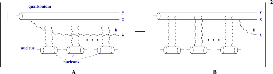
FIG. 1.: Diagrams contributing to the diffractive gluon production cross section in the quarkonium-nucleus scattering.

We are going to perform our calculations of $d{\hat{\sigma}}^{q{\bar{q}}A}_{diff}/d^{2}k\,dy$ in the time-ordered light cone perturbation theory [34] working in the light cone gauge of the projectile hadron $A_{+}=0$ [17]. Similarly to [17, 19, 21, 30, 31] we distinguish the cases when the gluon is present in the quarkonium’s wave function before the collision and when it is emitted after the collision. The diagrams contributing to the diffractive gluon production are shown in Fig. 1. We assume that the quark and the antiquark in the quarkonium are in the color singlet state, that is there is no soft non-perturbative partons which may carry some of the color in the quarkonium wave function making the $q\bar{q}$ pair non-singlet in color. The graph in Fig. 1A represents the case when the $q{\bar{q}}$ state develops a gluon fluctuation long before hitting the target. Subsequently quark, antiquark and the gluon rescatter in the target nucleus leaving it intact since we are interested in diffractive processes [29, 30]. The exchanged gluons coming from the nucleons in the nucleus can connect to either quark, antiquark or gluon lines and we have to sum over all of these possibilities. This is represented in Fig. 1 by not connecting gluon lines specifically to any of the projectile parton lines. The diagram in Fig. 1B corresponds to the case when only $q{\bar{q}}$ pair rescatters in the nucleus and the gluon is emitted after the scattering. Again both the quark and the antiquark lines interact with the nucleus which is represented by the gluon lines not connecting to any specific quark line. Finally in the diagrams of Fig. 1 the gluon is shown to be emitted off one of the quark lines only. To obtain the answer one of course has to sum over all possible gluon emissions off the quark and antiquark lines in the amplitude and in the complex conjugate amplitude.

To calculate the diagrams in Fig. 1 one needs to know forward “propagators” of the $q{\bar{q}}$ and $q{\bar{q}}G$ states through the nucleus. The propagator of the quark-antiquark state through the nucleus is well known and is given by [13, 17, 21, 30, 31]

$$\exp\left(-\frac{C_{F}}{4\,N_{c}}\,({\underline{x}}-{\underline{y}})^{2}\,Q_{s}^{2}\right)$$ (2)

where ${\underline{x}}$ and ${\underline{y}}$ are the transverse coordinates of the quark and the antiquark correspondingly and we have used a shorthand notation [26, 17, 21]

$$({\underline{x}}-{\underline{y}})^{2}Q_{s}^{2}\,=\,({\underline{x}}-{\underline{y}})^{2}\ \frac{8\pi^{2}\alpha_{s}N_{c}\sqrt{R^{2}-b^{2}}}{N^{2}_{c}-1}\,\rho\,xG(x,1/|{\underline{x}}-{\underline{y}}|^{2}),$$ (3)

with $\rho=A/[(4/3)\pi R^{3}]$ the density of the atomic number $A$ and ${\underline{b}}$ the impact parameter of the $q{\bar{q}}$ pair. Here the nucleus is assumed to be a sphere of radius $R$, but the result could be easily generalized to other geometries. The gluon distribution function in Eq. (3) at the two gluon level is given by [26]

$$xG(x,1/{\underline{x}}^{2})\ =\ \frac{\alpha_{s}C_{F}}{\pi}\,\ln\frac{1}{{\underline{x}}^{2}\mu^{2}},$$ (4)

with $\mu$ some infrared cutoff. In principle the saturation scale $Q_{s}$ has to be found from the implicit equation

$$Q_{s}^{2}(b)\ =\ \frac{8\pi^{2}\alpha_{s}N_{c}\sqrt{R^{2}-b^{2}}}{N^{2}_{c}-1}\,\rho\,xG(x,Q_{s}^{2}(b)).$$ (5)

Since the gluon distribution of Eq. (4) is a slowly (logarithmically) varying function of transverse distance in certain problems the $Q_{s}$ dependence on the right hand side of Eq. (5) could be neglected turning Eq. (5) from equation into an equality.

The “propagator” of the $q{\bar{q}}G$ state through the nucleus is a little harder to calculate. To do this let us consider the interaction between the $q{\bar{q}}G$ state and the first nucleon in the nucleus that exchanges gluons with it. The diagrams we need to sum are depicted in Fig. 2. To write down the contributions of these diagrams let us first introduce the gluon-nucleon interaction potential as a Fourier transform into coordinate space of the normalized gluon-nucleon scattering amplitude $\frac{1}{\sigma}\,\frac{d\sigma}{d^{2}l}$ [26, 17]

$${\tilde{V}}({\underline{x}})\,=\,\int d^{2}le^{-i{\underline{l}}\cdot{\underline{x}}}\,\frac{1}{\sigma}\,\frac{d\sigma}{d^{2}l}.$$ (6)

With the help of Eq. (6) one can easily see that the contributions of diagrams in Fig. 2 are

$$A\,=\,-\frac{C_{F}}{2N_{c}}\,{\tilde{V}}({\underline{0}})$$ (8)

$$B\,=\,-\frac{N_{c}}{2N_{c}}\,{\tilde{V}}({\underline{0}})$$ (9)

$$C\,=\,\frac{N_{c}}{2N_{c}}\,{\tilde{V}}({\underline{z}}-{\underline{x}})$$ (10)

$$D\,=\,\frac{N_{c}}{2N_{c}}\,{\tilde{V}}({\underline{z}}-{\underline{y}})$$ (11)

$$E\,=\,-\frac{1}{2N_{c}^{2}}\,{\tilde{V}}({\underline{x}}-{\underline{y}})$$ (12)

$$F\,=\,-\frac{C_{F}}{2N_{c}}\,{\tilde{V}}({\underline{0}})$$ (13)

where we take a trace in the color space of the nucleons and average over the colors of the nucleon, which yields a factor of $1/2N_{c}$.

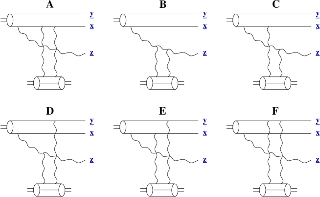
FIG. 2.: Diagrams included in a diffractive scattering of the $q{\bar{q}}G$ state on a single nucleon in the target nucleus.

Summing up the diagrams of Fig. 2 we obtain

$$A+B+\ldots+F\,=\,-\frac{1}{2}\,[{\tilde{V}}({\underline{0}})-{\tilde{V}}({\underline{x}}-{\underline{z}})]\,-\,\frac{1}{2}\,[{\tilde{V}}({\underline{0}})-{\tilde{V}}({\underline{y}}-{\underline{z}})]+\frac{1}{2N_{c}^{2}}[{\tilde{V}}({\underline{0}})-{\tilde{V}}({\underline{x}}-{\underline{y}})].$$ (14)

The calculation which led to Eq. (14) never assumed summation over the colors of the quark-antiquark pair and the gluon. Eqs. (II A) explicitly show us that diffractive scattering on a nucleon does not change the color structure of the incoming $q{\bar{q}}G$ state. This allows us to easily see that the full answer for the “propagator” of the $q{\bar{q}}G$ state through the nucleus could be obtained by just exponentiating the interaction with a single nucleon. Multiplying the right hand side of Eq. (14) by $2\sqrt{R^{2}-b^{2}}\,\rho\,\sigma$ to take into account the density of the nucleons in the nucleus [17] yields

$$-P({\underline{x}},{\underline{y}},{\underline{z}})\,\equiv\,2\sqrt{R^{2}-b^{2}}\,\rho\,\sigma\,(A+B+\ldots+F)\,=\,-\frac{1}{8}\,({\underline{x}}-{\underline{z}})^{2}Q_{s}^{2}-\frac{1}{8}\,({\underline{y}}-{\underline{z}})^{2}Q_{s}^{2}+\frac{1}{8N_{c}^{2}}\,({\underline{x}}-{\underline{y}})^{2}Q_{s}^{2}.$$ (15)

Exponentiating Eq. (15) we obtain the propagator of the $q{\bar{q}}G$ state through the nucleus

$$\exp\left(-P({\underline{x}},{\underline{y}},{\underline{z}})\right)\,=\,\exp\left(-\frac{1}{8}\,({\underline{x}}-{\underline{z}})^{2}Q_{s}^{2}-\frac{1}{8}\,({\underline{y}}-{\underline{z}})^{2}Q_{s}^{2}+\frac{1}{8N_{c}^{2}}\,({\underline{x}}-{\underline{y}})^{2}Q_{s}^{2}\right),$$ (16)

which agrees with the result derived by Kopeliovich et al in [18] and by Kovner and Wiedemann in [31].

Now it is straightforward to write down the cross section for diffractive gluon production. The cross section is given by the square of the amplitude depicted in Fig. 1 in momentum space. Fixing the overall normalization yields

$$\frac{d{\hat{\sigma}}^{q{\bar{q}}A}_{diff}}{d^{2}k\,dy}\,=\,\frac{\alpha_{s}C_{F}}{\pi^{2}}\,\frac{1}{(2\pi)^{2}}\,\int\,d^{2}b\,d^{2}z_{1}\,d^{2}z_{2}\,e^{-i{\underline{k}}\cdot({\underline{z}}_{1}-{\underline{z}}_{2})}\,\left(\frac{{\underline{z}}_{1}-{\underline{x}}}{|{\underline{z}}_{1}-{\underline{x}}|^{2}}-\frac{{\underline{z}}_{1}-{\underline{y}}}{|{\underline{z}}_{1}-{\underline{y}}|^{2}}\right)\cdot\left(\frac{{\underline{z}}_{2}-{\underline{x}}}{|{\underline{z}}_{2}-{\underline{x}}|^{2}}-\frac{{\underline{z}}_{2}-{\underline{y}}}{|{\underline{z}}_{2}-{\underline{y}}|^{2}}\right)$$

$$\times\left(e^{-P({\underline{x}},{\underline{y}},{\underline{z}}_{1})}-e^{-\frac{C_{F}}{4\,N_{c}}\,({\underline{x}}-{\underline{y}})^{2}\,Q_{s}^{2}}\right)\,\left(e^{-P({\underline{x}},{\underline{y}},{\underline{z}}_{2})}-e^{-\frac{C_{F}}{4\,N_{c}}\,({\underline{x}}-{\underline{y}})^{2}\,Q_{s}^{2}}\right),$$ (17)

where $z_{1}$ and $z_{2}$ are the transverse coordinates of the gluon in the amplitude and in the complex conjugate amplitude correspondingly. Eq. (17) gives us the cross section of diffractive gluon production in quarkonium-nucleus collisions. In general the integrals over $z_{1}$ and $z_{2}$ in Eq. (17) are very hard to do analytically and they should probably be done numerically. However, for not very large transverse momentum of the produced gluon, $k_{\perp}{{}_{\displaystyle{<}}\atop\displaystyle{\sim}}Q_{s}$, one can neglect the logarithmic dependence on $|{\underline{x}}-{\underline{y}}|$ of the gluon distribution in Eq. (3) making analytical evaluation of the integral in Eq. (17) possible [17, 21]. To calculate the integrals in Eq. (17) in this logarithmic approximation we need to estimate the following integral

$$I({\underline{k}},{\underline{x}};{\underline{y}})\,=\,\int\,d^{2}z\,e^{-i{\underline{k}}\cdot{\underline{z}}}\,\frac{{\underline{z}}-{\underline{x}}}{|{\underline{z}}-{\underline{x}}|^{2}}\,e^{-\frac{1}{8}\,({\underline{z}}-{\underline{x}})^{2}Q_{s}^{2}-\frac{1}{8}\,({\underline{z}}-{\underline{y}})^{2}Q_{s}^{2}}.$$ (18)

After redefinition of variables ${\underline{z}}\rightarrow{\underline{z}}+{\underline{x}}$ the integral of Eq. (18) could be rewritten as

$$I({\underline{k}},{\underline{x}};{\underline{y}})\,=\,ie^{-i{\underline{k}}\cdot{\underline{x}}-\frac{1}{8}\,({\underline{x}}-{\underline{y}})^{2}Q_{s}^{2}}\nabla_{k}\int_{0}^{\infty}\,\frac{dz}{z}\,e^{-\frac{1}{4}z^{2}Q_{s}^{2}}\,\int_{0}^{2\pi}\,d\phi\,e^{-ikz\cos\phi-\frac{1}{4}z|{\underline{x}}-{\underline{y}}|Q_{s}^{2}\cos(\phi-\beta)}$$ (19)

with $\phi$ the angle between ${\underline{z}}$ and ${\underline{k}}$ and $\beta$ the angle between ${\underline{z}}$ and ${\underline{x}}-{\underline{y}}$. The integration over $\phi$ in Eq. (19) could be done (see ${\bf 3.937}.2$ in [35]) yielding

$$I({\underline{k}},{\underline{x}};{\underline{y}})\,=\,2\pi ie^{-i{\underline{k}}\cdot{\underline{x}}-\frac{1}{8}\,({\underline{x}}-{\underline{y}})^{2}Q_{s}^{2}}\nabla_{k}\int_{0}^{\infty}\,\frac{dz}{z}\,e^{-\frac{1}{4}z^{2}Q_{s}^{2}}\,I_{0}(z\sqrt{-{\underline{\lambda}}^{2}}),$$ (20)

where we have introduced a two dimensional complex vector

$${\underline{\lambda}}\,=\,{\underline{k}}-\frac{i}{4}\,Q_{s}^{2}\,({\underline{x}}-{\underline{y}}).$$ (21)

Differentiating Eq. (20) over $k$ and integrating over $z$ we finally obtain

$$I({\underline{k}},{\underline{x}};{\underline{y}})\,=\,-2\pi i\,\frac{{\underline{\lambda}}}{{\underline{\lambda}}^{2}}\,\left(1-e^{-{\underline{\lambda}}^{2}/Q_{s}^{2}}\right)\,e^{-i{\underline{k}}\cdot{\underline{x}}-\frac{1}{8}\,({\underline{x}}-{\underline{y}})^{2}Q_{s}^{2}}.$$ (22)

Inserting Eq. (15) into Eq. (17) and employing Eq. (22) yields

$$\frac{d{\hat{\sigma}}^{q{\bar{q}}A}_{diff}}{d^{2}k\,dy}\,=\,\frac{\alpha_{s}C_{F}}{\pi^{2}}\,\int\,d^{2}b\,\left|\frac{{\underline{\lambda}}}{{\underline{\lambda}}^{2}}\,\left(1-e^{-{\underline{\lambda}}^{2}/Q_{s}^{2}}\right)\,e^{-i{\underline{k}}\cdot{\underline{x}}}-\frac{{\underline{\lambda}}^{*}}{{\underline{\lambda}}^{*2}}\,\left(1-e^{-{\underline{\lambda}}^{*2}/Q_{s}^{2}}\right)\,e^{-i{\underline{k}}\cdot{\underline{y}}}\right.$$

$$-\left.\frac{{\underline{k}}}{{\underline{k}}^{2}}\,\left(e^{-i{\underline{k}}\cdot{\underline{x}}}-e^{-i{\underline{k}}\cdot{\underline{y}}}\right)\right|^{2}\,e^{-\frac{C_{F}}{2\,N_{c}}({\underline{x}}-{\underline{y}})^{2}Q_{s}^{2}},$$ (23)

where ${\underline{\lambda}}^{*}$ is the complex conjugate of ${\underline{\lambda}}$.

Eq. (23) together with Eq. (21) provides us with the expression for the diffractive gluon production cross section for quarkonium-nucleus collisions explicitly in terms of gluon’s transverse momentum ${\underline{k}}$ and the transverse separation of the onium state ${\underline{x}}-{\underline{y}}$. After integration over angles between ${\underline{k}}$ and ${\underline{x}}-{\underline{y}}$ Eq. (23) could be easily rewritten in terms of the invariant mass of the produced particles which is approximately equal to $M_{X}^{2}\approx{\underline{k}}^{2}/x$ where $y=\ln 1/x$.

To the degree that a quarkonium state can serve as a model of a baryon projectile such as proton, Eqs. (17) and (23) could describe the diffractive gluon production cross section in $pA$ collisions. However, a much better model of $pA$ collisions would involve a realistic proton consisting of three valence quarks and we are going to address this problem in Sect. IIB.

B Proton–Nucleus Collisions

Diffractive gluon production in proton-nucleus collisions is different from our previous discussion of onium-nucleus scattering only by the fact that the proton consists of three valence quarks instead of quark-antiquark pair. Again we assume that the three quarks in the proton are in a color singlet state by themselves, i.e., there is no soft non-perturbative gluons in the proton’s wave function to modify this picture.

Similarly to the quarkonium case diffractive gluon production cross section could be expressed as a convolution of the proton’s wave function and the diffractive cross section of a $qqq$ state on the target nucleus:

$$\frac{d\sigma^{pA}_{diff}}{d^{2}k\,dy}\,=\,\int d^{2}x_{13}\,d^{2}x_{23}\,d\alpha_{1}\,d\alpha_{2}\,|\Psi^{p}({\underline{x}}_{13},{\underline{x}}_{23},\alpha_{1},\alpha_{2})|^{2}\,\frac{d{\hat{\sigma}}^{qqqA}_{diff}}{d^{2}k\,dy}({\underline{x}}_{13},{\underline{x}}_{23}),$$ (24)

with ${\underline{x}}_{13},{\underline{x}}_{23}$ the distances between valence quarks in the proton and $\alpha_{1},\alpha_{2}$ light cone fractions of the proton’s momentum carried by two of the quarks.

The diagrams describing the diffractive gluon production in pA are shown in Fig. 3. They are similar to the onium-nucleus scattering diagrams of Fig. 1 with three quarks instead of $q\bar{q}$ pair in the projectile. The diagrams in Fig. 3 demonstrate that in order to calculate diffractive gluon production cross section we need to know the diffractive “propagators” of the $qqq$ and $qqqG$ states through the nucleus.

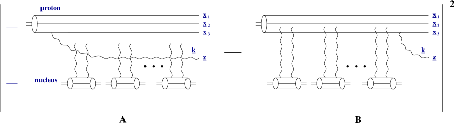
FIG. 3.: Diffractive gluon production in proton-nucleus scattering (pA).

First we are going to calculate the “propagator” of the $qqq$ state through the nucleus, which is needed for the diagram in Fig. 3B. Similar to what was done in Sect. IIA we need to consider scattering of three quarks on a single nucleon. The contributing diagrams are shown in Fig. 4. There are two types of diagrams in proton-nucleon interaction: there are diagrams where both gluons connect to the same quark line, as shown in Fig. 4A and there are diagrams where gluons connect to different quark lines, as shown in Fig. 4B. The color singlet configuration of three quarks is achieved by antisymmetrization over their color indices with the help of $\epsilon_{\alpha\beta\gamma}$.

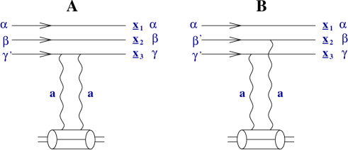
FIG. 4.: Diagrams contributing to the interaction of the proton with a nucleon in the target nucleus.

The diagram in Fig. 4A easily yields

$${\cal A}\,=\,-\frac{C_{F}}{2N_{c}}\,{\tilde{V}}({\underline{0}}).$$ (25)

The diagram in Fig. 4B is a little harder to calculate. The color factor there is given by

$$\frac{1}{2N_{c}}\,\epsilon_{\alpha\beta^{\prime}\gamma^{\prime}}\,(T^{a})_{\beta\beta^{\prime}}\,(T^{a})_{\gamma\gamma^{\prime}}.$$

Using the Fierz identity

$$(T^{a})_{\alpha\beta}\,(T^{a})_{\gamma\delta}\,=\,\frac{1}{2}\,\delta_{\alpha\delta}\,\delta_{\beta\gamma}-\,\frac{1}{2N_{c}}\,\delta_{\alpha\beta}\,\delta_{\gamma\delta}$$ (26)

we readily evaluate the diagram in Fig. 4B to be

$${\cal B}\,=\,\frac{N_{c}+1}{(2N_{c})^{2}}\,{\tilde{V}}({\underline{x}}_{3}-{\underline{x}}_{2}).$$ (27)

To obtain the proton’s propagator out of Eqs. (25) and (27) we have to sum over gluons’ connections to all valence quarks in the proton and multiply the result by $2\sqrt{R^{2}-b^{2}}\,\rho\,\sigma$. The final expression for the proton’s propagator is

$$\exp\left(-\frac{N_{c}+1}{4\,(2N_{c})^{2}}\,\sum_{i,j=1;i\neq j}^{N_{c}}\,({\underline{x}}_{i}-{\underline{x}}_{j})^{2}Q_{s}^{2}\right)$$ (28)

which for the case of three colors becomes

$$\exp\left(-\frac{1}{18}\,\left[({\underline{x}}_{1}-{\underline{x}}_{2})^{2}Q_{s}^{2}+({\underline{x}}_{2}-{\underline{x}}_{3})^{2}Q_{s}^{2}+({\underline{x}}_{1}-{\underline{x}}_{3})^{2}Q_{s}^{2}\right]\right).$$ (29)

Calculation of the $qqqG$ “propagator” in the nucleus is more complicated because, unlike the above cases, the scattering of a single nucleon is not diagonal in the color space. Thus instead of exponentiating a scalar we will have to exponentiate a matrix in the color space. (For similar calculations of different quantities see [31].) To determine the color matrix we have to again consider the scattering of the $qqqG$ system on a single nucleon. First let us note that the $qqqG$ system can arise due to gluon emissions off each of the valence quarks, giving rise to a different color structure in each case. The possibilities are outlined in Fig. 5. Quarks there are labeled $1,2,3$ carrying color indices $\alpha,\beta,\gamma$ correspondingly.

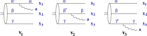
FIG. 5.: Three possible ways of generating a $qqqG$ fluctuation in a proton.

The three states depicted in Fig. 5 correspond to three color matrices, which we will label $v_{1}$, $v_{2}$ and $v_{3}$ such that

$$v_{1}\,=\,\frac{1}{\sqrt{6}}\,\epsilon_{\alpha^{\prime}\beta\gamma}\,(T^{a})_{\alpha\alpha^{\prime}},\hskip 28.45274ptv_{2}\,=\,\frac{1}{\sqrt{6}}\,\epsilon_{\alpha\beta^{\prime}\gamma}\,(T^{a})_{\beta\beta^{\prime}},\hskip 28.45274ptv_{3}\,=\,\frac{1}{\sqrt{6}}\,\epsilon_{\alpha\beta\gamma^{\prime}}\,(T^{a})_{\gamma\gamma^{\prime}}.$$ (30)

The factor of $1/\sqrt{6}$ is arises in Eq. (30) due to $(\epsilon_{\alpha\beta\gamma})^{2}=N_{c}!=6$ and is included to factor out the color structure of the proton’s wave function.

As we will see below interactions with nucleons only transform each of the states in Eq. (30) into linear combinations of the others. It is therefore convenient to make an orthonormal basis out of these matrices. We note that since due to $SU(N_{c})$ group properties

$$v_{1}+v_{2}+v_{3}=0$$ (31)

the matrices of Eq. (30) are not linearly independent. (In fact they represent the roots of $SU(N_{c})$.) We are going to choose the following orthonormal basis

$$u_{2}=v_{2}+\frac{1}{2}\,v_{3},\hskip 28.45274ptu_{3}=\frac{\sqrt{3}}{2}\,v_{3},$$ (32)

where we have explicitly inserted $N_{c}=3$ and $C_{F}=4/3$. Since in Fig. 5 we explicitly consider a baryon (proton) consisting of three valence quarks our results from here to the end of the section will be derived for $N_{c}=3$. To generalize this discussion to an arbitrary $N_{c}$ one would have to introduce $N_{c}$ different matrices $v_{1},\ldots,v_{N_{c}}$ and work in the $N_{c}-1$ dimensional space of the orthogonal basis $u_{2},\ldots,u_{N_{c}}$. Doing that is beyond the scope of this paper.

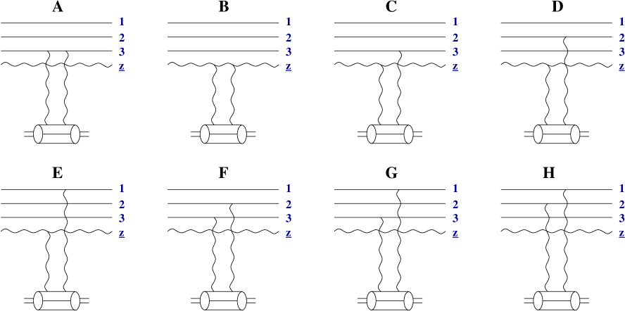
FIG. 6.: Interaction of the $qqqG$ state with a nucleon.

Let us now consider interaction of the $qqqG$ state with a single nucleon in the nucleus. The corresponding diagrams are depicted in Fig. 6. Each of the diagrams is a matrix in the $u_{2},u_{3}$ linear space. To calculate the diagrams of Fig. 6 we have to first calculate the action of each of them on $v_{2}$ and $v_{3}$ and then use Eq. (32) to rewrite their contributions in the $(u_{2},u_{3})$ basis. The result of a rather tedious calculation yields

$$M_{A}\,=\,-\frac{2}{3}\,{\tilde{V}}({\underline{0}})\pmatrix{1&0\cr 0&1}$$ (34)

$$M_{B}\,=\,-\frac{1}{2}\,{\tilde{V}}({\underline{0}})\pmatrix{1&0\cr 0&1}$$ (35)

$$M_{C}\,=\,\frac{1}{2}\,{\tilde{V}}({\underline{z}}-{\underline{x}}_{3})\pmatrix{1/3&0\cr 0&1}$$ (36)

$$M_{D}\,=\,\frac{1}{4}\,{\tilde{V}}({\underline{z}}-{\underline{x}}_{2})\pmatrix{5/3&-1/\sqrt{3}\cr-1/\sqrt{3}&1}$$ (37)

$$M_{E}\,=\,\frac{1}{4}\,{\tilde{V}}({\underline{z}}-{\underline{x}}_{1})\pmatrix{5/3&1/\sqrt{3}\cr 1/\sqrt{3}&1}$$ (38)

$$M_{F}\,=\,\frac{1}{4}\,{\tilde{V}}({\underline{x}}_{2}-{\underline{x}}_{3})\pmatrix{5/9&1/\sqrt{3}\cr 1/\sqrt{3}&-1/9}$$ (39)

$$M_{G}\,=\,\frac{1}{4}\,{\tilde{V}}({\underline{x}}_{1}-{\underline{x}}_{3})\pmatrix{5/9&-1/\sqrt{3}\cr-1/\sqrt{3}&-1/9}$$ (40)

$$M_{H}\,=\,{\tilde{V}}({\underline{x}}_{1}-{\underline{x}}_{2})\pmatrix{-1/9&0\cr 0&2/9}$$ (41)

where in Eq. (34) we summed over gluon connections to all three valence quarks. Summing up the contributions of Eq. (6) and multiplying them by $2\sqrt{R^{2}-b^{2}}\,\rho\,\sigma$ yields

$$-M({\underline{z}})\,\equiv\,2\sqrt{R^{2}-b^{2}}\,\rho\,\sigma\,(M_{A}+\ldots+M_{H})$$ (42)

with the matrix $M({\underline{z}})$ given by

$$M({\underline{z}})\,=\,\pmatrix{\frac{1}{6}\,\zeta_{3}+\frac{5}{12}\,(\zeta_{2}+\zeta_{1})+\frac{5}{36}\,(\chi_{23}+\chi_{13})-\frac{1}{9}\,\chi_{12}&\frac{1}{4\sqrt{3}}\,(-\zeta_{2}+\zeta_{1}+\chi_{23}-\chi_{13})\cr\frac{1}{4\sqrt{3}}\,(-\zeta_{2}+\zeta_{1}+\chi_{23}-\chi_{13})&\frac{1}{2}\,\zeta_{3}+\frac{1}{4}\,(\zeta_{2}+\zeta_{1})-\frac{1}{36}\,(\chi_{23}+\chi_{13})+\frac{2}{9}\,\chi_{12}}$$ (43)

where we have defined

$$\zeta_{i}\,\equiv\,\frac{1}{4}\,({\underline{z}}-{\underline{x}}_{i})^{2}Q_{s}^{2}$$ (44)

and

$$\chi_{ij}\,\equiv\,\frac{1}{4}\,({\underline{x}}_{i}-{\underline{x}}_{j})^{2}Q_{s}^{2}.$$ (45)

The “propagator” of the $qqqG$ state through the nucleus is given by

$$\exp[-M({\underline{z}})],$$ (46)

which is also a matrix.

Now we are in a position to write down a compact expression for the diffractive gluon production cross section in the proton-nucleus collisions. The initial proton state in the amplitude and in the complex conjugate amplitude could be in either one of the three states, $v_{1}$, $v_{2}$ and $v_{3}$, which are given by

$$v_{1}^{T}\,=\,(-1\hskip 5.69054pt,\hskip 8.53581pt-\frac{1}{\sqrt{3}}),\hskip 28.45274ptv_{2}^{T}\,=\,(1\hskip 5.69054pt,\hskip 8.53581pt-\frac{1}{\sqrt{3}}),\hskip 28.45274ptv_{3}^{T}\,=\,(0\hskip 5.69054pt,\hskip 8.53581pt\frac{2}{\sqrt{3}})$$ (47)

in the $(u_{2},u_{3})$ basis. If the proton in the amplitude is in the state $v_{i}$ and in the complex conjugate amplitude it is in the state $v_{j}$ we can define a diffractive overlap functions

$$\Pi_{ij}\,\equiv\,v_{i}^{T}\left(e^{-M({\underline{z}}_{1})}-e^{-(2/9)(\chi_{12}+\chi_{13}+\chi_{23})}\right)\left(e^{-M({\underline{z}}_{2})}-e^{-(2/9)(\chi_{12}+\chi_{13}+\chi_{23})}\right)v_{j},$$ (48)

where, as in Sect. IIA , ${\underline{z}}_{1}$ and ${\underline{z}}_{2}$ are the gluon’s transverse coordinates in the amplitude and in the complex conjugate amplitude. The second exponent in Eq. (48) comes from Fig. 3B with the propagator of the proton in the nucleus given by Eq. (29), which is a unit matrix in the $(u_{2},u_{3})$ color space. The diffractive gluon production cross section in pA can be written in terms of $\Pi_{ij}$’s as

$$\frac{d{\hat{\sigma}}^{qqqA}_{diff}}{d^{2}k\,dy}\,=\,\frac{\alpha_{s}}{(2\pi)^{2}\,\pi^{2}}\,\int\,d^{2}b\,d^{2}z_{1}\,d^{2}z_{2}\,\sum_{i=1}^{3}\sum_{j=1}^{3}\frac{{\underline{z}}_{1}-{\underline{x}}_{i}}{|{\underline{z}}_{1}-{\underline{x}}_{i}|^{2}}\cdot\frac{{\underline{z}}_{2}-{\underline{x}}_{j}}{|{\underline{z}}_{2}-{\underline{x}}_{j}|^{2}}\,\Pi_{ij}.$$ (49)

Eqs. (43), (47), (48), (49), together with Eq. (24) provide us the answer for diffractive gluon production cross section in pA collisions. The matrix expression for $\Pi_{ij}$ in Eq. (48) could be rewritten in the usual “scalar” form. After some lengthy algebra one arrives at

$$\Pi_{33}\,=\,\frac{4}{3}\,\left[4\frac{M_{12}({\underline{z}}_{1})M_{12}({\underline{z}}_{2})}{\sqrt{D({\underline{z}}_{1})\,D({\underline{z}}_{2})}}\,e^{-\frac{1}{2}\,[M_{11}({\underline{z}}_{1})+M_{22}({\underline{z}}_{1})+M_{11}({\underline{z}}_{2})+M_{22}({\underline{z}}_{2})]}\,\sinh\frac{\sqrt{D({\underline{z}}_{1})}}{2}\,\sinh\frac{\sqrt{D({\underline{z}}_{2})}}{2}\right.$$

$$+\left(e^{-\frac{1}{2}\,[M_{11}({\underline{z}}_{1})+M_{22}({\underline{z}}_{1})]}\,R({\underline{z}}_{1})-e^{-\frac{2}{9}\,(\chi_{12}+\chi_{23}+\chi_{13})}\right)\left.\left(e^{-\frac{1}{2}\,[M_{11}({\underline{z}}_{2})+M_{22}({\underline{z}}_{2})]}\,R({\underline{z}}_{2})-e^{-\frac{2}{9}\,(\chi_{12}+\chi_{23}+\chi_{13})}\right)\right]$$ (50)

and

$$\Pi_{23}\,=\,-\frac{4}{\sqrt{3}}\,\frac{M_{12}({\underline{z}}_{2})}{\sqrt{D({\underline{z}}_{2})}}\,e^{-\frac{1}{2}\,[M_{11}({\underline{z}}_{2})+M_{22}({\underline{z}}_{2})]}\,\sinh\frac{\sqrt{D({\underline{z}}_{2})}}{2}$$

$$\times\left(e^{-\frac{1}{2}\,[M_{11}({\underline{z}}_{1})+M_{22}({\underline{z}}_{1})]}\,L({\underline{z}}_{1})-e^{-\frac{2}{9}\,(\chi_{12}+\chi_{23}+\chi_{13})}+\frac{2}{\sqrt{3}}\,\frac{M_{12}({\underline{z}}_{1})}{\sqrt{D({\underline{z}}_{1})}}\,e^{-\frac{1}{2}\,[M_{11}({\underline{z}}_{1})+M_{22}({\underline{z}}_{1})]}\,\sinh\frac{\sqrt{D({\underline{z}}_{1})}}{2}\right)$$

$$-\frac{2}{\sqrt{3}}\,\left(e^{-\frac{1}{2}\,[M_{11}({\underline{z}}_{2})+M_{22}({\underline{z}}_{2})]}\,R({\underline{z}}_{2})-e^{-\frac{2}{9}\,(\chi_{12}+\chi_{23}+\chi_{13})}\right)\,\left(\frac{2\,M_{12}({\underline{z}}_{1})}{\sqrt{D({\underline{z}}_{1})}}\,e^{-\frac{1}{2}\,[M_{11}({\underline{z}}_{1})+M_{22}({\underline{z}}_{1})]}\,\sinh\frac{\sqrt{D({\underline{z}}_{1})}}{2}\right.$$

$$-\left.\frac{1}{\sqrt{3}}\,e^{-\frac{2}{9}\,(\chi_{12}+\chi_{23}+\chi_{13})}+\frac{1}{\sqrt{3}}\,e^{-\frac{1}{2}\,[M_{11}({\underline{z}}_{1})+M_{22}({\underline{z}}_{1})]}\,R({\underline{z}}_{1})\right),$$ (51)

where we have introduced

$$D({\underline{z}})\,\equiv\,4\,[M_{12}({\underline{z}})]^{2}+[M_{11}({\underline{z}})-M_{22}({\underline{z}})]^{2},$$ (52)

$$R({\underline{z}})\,\equiv\,\cosh\frac{\sqrt{D({\underline{z}})}}{2}+\frac{M_{11}({\underline{z}})-M_{22}({\underline{z}})}{\sqrt{D({\underline{z}})}}\,\sinh\frac{\sqrt{D({\underline{z}})}}{2},$$ (53)

$$L({\underline{z}})\,\equiv\,\cosh\frac{\sqrt{D({\underline{z}})}}{2}-\frac{M_{11}({\underline{z}})-M_{22}({\underline{z}})}{\sqrt{D({\underline{z}})}}\,\sinh\frac{\sqrt{D({\underline{z}})}}{2},$$ (54)

and $M_{11}({\underline{z}})$, $M_{22}({\underline{z}})$ and $M_{12}({\underline{z}})$ are the components of (symmetric) matrix $M({\underline{z}})$ given in Eq. (43). All other diagonal ($\Pi_{ii}$) and off-diagonal ($\Pi_{ij}$, $i\neq j$) propagators could be obtained from Eqs. (50) and (51) correspondingly by appropriate permutations of the indices of $\zeta$’s and $\chi$’s.

We have calculated above the diffractive gluon production cross section for quarkonium-nucleus and proton-nucleus collisions in the quasi-classical approximation (Eqs. (17) and (49)). The calculation for the case of pA collisions is much more sophisticated than the calculation for onium-nucleus scattering. This is due to the fact that the object in question is the diffractive cross section and therefore interactions with spectator quarks have to be included. When one calculates the total inclusive gluon production cross section the interactions of the target nucleus with the spectator quarks (or gluons) in the projectile disappear due to real-virtual cancellations [17, 18, 19, 31]. All one has to do there to obtain the answer is to calculate the interaction of a single projectile quark with the nucleus and then convolute it with the quark distribution function in the proton [17, 18, 19, 31]. This is not the case for diffractive scattering: since the final state here is not “inclusive”, i.e., we imposed a rapidity gap condition on the final state, only virtual exchanges contribute to interaction with the target, as seen in Figs. 1 and 3. Therefore there is no real-virtual cancellation for interactions with spectator quarks (quarks off which the gluon was not emitted neither in the amplitude nor in the complex conjugate amplitude). Interactions with all partons in the proton’s or onium’s wave function have to be included. That way, since our results of Eqs. (17) and (49) were derived for the models of hadrons consisting of valence quarks one should use them to describe the experimental data with caution. Realistic hadron’s wave function at high energy may include non-perturbative fluctuations producing the so-called “intrinsic” sea quarks advocated by Brodsky et al in [36] and quantum fluctuations due to perturbative QCD evolution producing (“extrinsic”) sea quarks and gluons. Inclusion of either one of the two effects would tremendously complicate the diffractive gluon production cross section calculations presented above. Inclusion of the effects of sea quarks and gluons in diffractive production cross section is an important question which has to be addresses in a separate study. At the moment we may argue that perturbatively generated sea quarks and gluons would bring in higher powers of the strong coupling constant $\alpha_{s}$ and could be neglected in the quasi-classical approach employed here.

III Deep Inelastic Scattering

We can generalize the results of Sect. IIA to the case of diffractive gluon production in the deep inelastic scattering (DIS). The diagrams important for the small-$x$ gluon production are the same diagrams as shown in Fig. 1 only with the wave function of a virtual photon splitting into $q\bar{q}$ pair instead of onium wave function. The expression for the diffractive gluon production cross section in DIS is

$$\frac{d\sigma^{\gamma^{*}A\rightarrow q{\bar{q}}GA}_{diff}}{d^{2}k\,dy}\,=\,\frac{1}{2\pi^{2}}\,\int\,d^{2}r\,dz\,\Phi^{\gamma^{*}\rightarrow q\bar{q}}({\underline{r}},z)\,\frac{d{\hat{\sigma}}^{q{\bar{q}}A}_{diff}}{d^{2}k\,dy}({\underline{r}}),$$ (55)

where $d{\hat{\sigma}}^{q{\bar{q}}A}_{diff}/d^{2}k\,dy$ is given by Eq. (17), ${\underline{r}}={\underline{x}}-{\underline{y}}$ is the transverse separation of the quark-antiquark pair and $z$ is the virtual photon’s light cone momentum fraction carried by the quark. The square of the virtual photon’s wave function $\Phi^{\gamma^{*}\rightarrow q\bar{q}}({\underline{r}},z)$ is a well known function and could be found for instance in [30].

An interesting question to address is the calculation of the inclusive gluon production cross section in DIS. This corresponds to the gluon production cross section without any restrictions on the final state of the target proton or nucleus. The problem is somewhat different from the gluon production in pA as discussed in [17, 18, 31]. In the model of the proton considered in [17, 18, 31] the interacting valence quark in the proton could have an arbitrary color in the initial state due to the soft intrinsic partons which would randomize the colors of valence quarks. Thus an independent summation was performed over the colors of this interacting quark. This could not be done in DIS: due to perturbative nature of the $q\bar{q}$ state at the leading order in $\alpha_{s}$ there is no quantum fluctuations in the $q\bar{q}$ wave function randomizing the colors of the quark and the antiquark. Instead, in quasi-classical approximation employed here the quark and antiquark are in the color singlet state and an independent summation over the colors of one of them is not possible. Therefore we have to consider the diagrams with the gluon emitted off both the quark and the antiquark.

There are two types of diagrams contributing to inclusive gluon production cross section in DIS. The diagrams may have the gluon emitted off the quark (antiquark) both in the amplitude and in the complex conjugate amplitude (symmetric diagrams) or they may have the gluon emitted off the quark (antiquark) in the amplitude and off the antiquark (quark) in the complex conjugate amplitude (asymmetric diagrams). The gluon production contribution in the diagrams of the first kind is exactly the same as in pA [17] (for a more detailed review see [21, 31]). The contribution of the second (asymmetric) type of diagrams differs from the first in: (i) the interference terms, where the gluon is emitted before the collision in the amplitude and after the collision in the complex conjugate amplitude and vice versa; (ii) the late emission time terms, where the gluon is emitted after the interaction both in the amplitude and in the complex conjugate amplitude. To understand (i) let us discuss a specific case of a gluon emitted off the quark line before the collision in the amplitude and absorbed by the antiquark line after the collision in the complex conjugate amplitude. There the interactions with the target nucleons in which at least one of the exchanged Coulomb gluon lines connects to the quark line cancel by real-virtual cancellation with the diagrams where that gluon line is on the other side of the cut. Only the interactions with the gluon and the antiquark lines survive and could be easily resummed along the lines outlined above and in [17]. The late emission time diagrams (ii) in the case of asymmetric gluon emission are different from their symmetric counterparts because the real-virtual cancellation of interactions here does not happen. The reason is the color factors which are now different for the “real” and “virtual” diagrams. Similar to [17] one has to consider the last nucleon interacting with the $q\bar{q}$ pair before the gluon emission. With the help of Fierz identity the interaction diagrams for this last nucleon could be resummed and prove to be diagonal in the color space, which simplifies their exponentiation. At the end the one gluon inclusive production cross section for DIS could be written as

$$\frac{d\sigma^{\gamma^{*}A\rightarrow q{\bar{q}}GA}_{incl}}{d^{2}k\,dy}\,=\,\frac{1}{2\pi^{2}}\,\int\,d^{2}r\,dz\,\Phi^{\gamma^{*}\rightarrow q\bar{q}}({\underline{r}},z)\,\frac{d{\hat{\sigma}}^{q{\bar{q}}A}_{incl}}{d^{2}k\,dy}({\underline{r}})$$ (56)

with

$$\frac{d{\hat{\sigma}}^{q{\bar{q}}A}_{incl}}{d^{2}k\,dy}({\underline{x}}-{\underline{y}})\,=\,\frac{\alpha_{s}C_{F}}{\pi^{2}}\,\frac{1}{(2\pi)^{2}}\,\int\,d^{2}b\,d^{2}z_{1}\,d^{2}z_{2}\,e^{-i{\underline{k}}\cdot({\underline{z}}_{1}-{\underline{z}}_{2})}\,\left[\frac{{\underline{z}}_{1}-{\underline{x}}}{|{\underline{z}}_{1}-{\underline{x}}|^{2}}\cdot\frac{{\underline{z}}_{2}-{\underline{x}}}{|{\underline{z}}_{2}-{\underline{x}}|^{2}}\right.\,\left(1-e^{-({\underline{z}}_{1}-{\underline{x}})^{2}Q_{s}^{2}/4}\right.$$

$$\left.-e^{-({\underline{z}}_{2}-{\underline{x}})^{2}Q_{s}^{2}/4}+e^{-({\underline{z}}_{1}-{\underline{z}}_{2})^{2}Q_{s}^{2}/4}\right)+\frac{{\underline{z}}_{1}-{\underline{y}}}{|{\underline{z}}_{1}-{\underline{y}}|^{2}}\cdot\frac{{\underline{z}}_{2}-{\underline{y}}}{|{\underline{z}}_{2}-{\underline{y}}|^{2}}\,\left(1-e^{-({\underline{z}}_{1}-{\underline{y}})^{2}Q_{s}^{2}/4}-e^{-({\underline{z}}_{2}-{\underline{y}})^{2}Q_{s}^{2}/4}\right.$$

$$+\left.e^{-({\underline{z}}_{1}-{\underline{z}}_{2})^{2}Q_{s}^{2}/4}\right)-\frac{{\underline{z}}_{1}-{\underline{x}}}{|{\underline{z}}_{1}-{\underline{x}}|^{2}}\cdot\frac{{\underline{z}}_{2}-{\underline{y}}}{|{\underline{z}}_{2}-{\underline{y}}|^{2}}\,\left(e^{-({\underline{x}}-{\underline{y}})^{2}Q_{s}^{2}/4}-e^{-({\underline{z}}_{1}-{\underline{y}})^{2}Q_{s}^{2}/4}-e^{-({\underline{z}}_{2}-{\underline{x}})^{2}Q_{s}^{2}/4}+e^{-({\underline{z}}_{1}-{\underline{z}}_{2})^{2}Q_{s}^{2}/4}\right)$$

$$\left.-\frac{{\underline{z}}_{1}-{\underline{y}}}{|{\underline{z}}_{1}-{\underline{y}}|^{2}}\cdot\frac{{\underline{z}}_{2}-{\underline{x}}}{|{\underline{z}}_{2}-{\underline{x}}|^{2}}\,\left(e^{-({\underline{x}}-{\underline{y}})^{2}Q_{s}^{2}/4}-e^{-({\underline{z}}_{1}-{\underline{x}})^{2}Q_{s}^{2}/4}-e^{-({\underline{z}}_{2}-{\underline{y}})^{2}Q_{s}^{2}/4}+e^{-({\underline{z}}_{1}-{\underline{z}}_{2})^{2}Q_{s}^{2}/4}\right)\right].$$ (57)

As one can easily check the cross section of Eq. (57) goes to zero in the limit of zero dipole size ${\underline{x}}\rightarrow{\underline{y}}$.

Eqs. (56) and (57) provide us with the one gluon inclusive production cross section in DIS calculated in the quasi-classical approximation and could be used to describe the pion or minijet production data at HERA.

REFERENCES

- [1] L. V. Gribov, E. M. Levin, and M. G. Ryskin, Phys. Rep. 100, 1 (1983); A.H. Mueller, J.-W. Qiu, Nucl. Phys. B268, 427 (1986).
- [2] L. McLerran and R. Venugopalan, Phys. Rev. D 49, 2233 (1994); 49, 3352 (1994); 50, 2225 (1994).
- [3] Yu.V. Kovchegov, Phys. Rev. D 54, 5463 (1996); 55, 5445 (1997).
- [4] J. Jalilian-Marian, A. Kovner, L. McLerran, and H. Weigert, Phys. Rev. D 55,5414 (1997).
- [5] Yu. V. Kovchegov, Phys. Rev. D 60, 034008 (1999); D 61, 074018 (2000).
- [6] I. I. Balitsky, Nucl. Phys. B463, 99 (1996).
- [7] A. H. Mueller, Nucl. Phys. B572, 227 (2000).
- [8] J. Jalilian-Marian, A. Kovner, A. Leonidov, and H. Weigert, Nucl. Phys. B 504, 415 (1997); Phys. Rev. D 59 014014 (1999); Phys. Rev. D59, 034007 (1999); J. Jalilian-Marian, A. Kovner, and H. Weigert, Phys. Rev. D 59 014015 (1999).
- [9] L. Frankfurt, V. Guzey and M. Strikman, J. Phys. G 27, R23 (2001) and references therein; Yu. V. Kovchegov and M. Strikman, hep-ph/0107015.
- [10] D. E. Kharzeev, Yu. V. Kovchegov, E. Levin, hep-ph/0106248.
- [11] V.S. Fadin and L.N. Lipatov, Phys. Lett. B429, 127 (1998); M. Ciafaloni and G. Camici, Phys. Lett. B430, 349 (1998) and references therein.
- [12] E.A. Kuraev, L.N. Lipatov and V.S. Fadin, Sov. Phys. JETP 45, 199 (1977); Ya.Ya. Balitsky and L.N. Lipatov, Sov. J. Nucl. Phys. 28, 22 (1978).
- [13] A.H. Mueller, Nucl. Phys. B335, 115 (1990).
- [14] A.H. Mueller, Nucl. Phys. B415, 373 (1994); A.H. Mueller and B. Patel, Nucl. Phys. B425, 471 (1994); A.H. Mueller, Nucl. Phys. B437, 107 (1995); Z. Chen, A.H. Mueller, Nucl. Phys. B451, 579 (1995).
- [15] A. Kovner, J. G. Milhano, H. Weigert, Phys. Rev. D 62, 114005 (2000); H. Weigert, hep-ph/0004044; M. Braun, Eur. Phys. J. C16, 337 (2000); E. Iancu, A. Leonidov, L. McLerran, hep-ph/0011241; hep-ph/0102009; E. Levin and K. Tuchin, Nucl. Phys. B573, 833 (2000); E. Levin and M. Lublinsky, hep-ph/0104108; M. Lublinsky,E. Gotsman, E. Levin and U. Maor, hep-ph/0102321.
- [16] A. Kovner, L. McLerran, and H. Weigert, Phys. Rev. D 52, 6231 (1995); 52, 3809 (1995); M. Gyulassy, L. McLerran, Phys. Rev. C 56, 2219 (1997); Yu.V. Kovchegov, D. H. Rischke, Phys. Rev. C 56, 1084 (1997); J.F. Gunion and G. Bertsch, Phys. Rev. D 25, 746 (1982).
- [17] Yu. V. Kovchegov, A.H. Mueller, Nucl. Phys. B529, 451 (1998).
- [18] B. Z. Kopeliovich, A. V. Tarasov, A. Schafer, Phys. Rev. C 59, 1609 (1999); B. Z. Kopeliovich, A. Schafer, A. V. Tarasov, Phys. Rev. D 62, 054022 (2000); B. Kopeliovich, A. Tarasov, J. Hufner, hep-ph/0104256.
- [19] A. Dumitru, L. McLerran, hep-ph/0105268.
- [20] A. Krasnitz, R. Venugopalan, Report No. hep-ph/0007108; Phys. Rev. Lett. 84, 4309 (2000); Nucl. Phys. B557, 237 (1999).
- [21] Yu. V. Kovchegov, hep-ph/0011252; hep-ph/0106313.
- [22] D. Kharzeev and M. Nardi, Phys. Lett. B507, 121 (2001).
- [23] Yu. V. Kovchegov, E. Levin, L. McLerran, Phys. Rev. C 63, 024903 (2001).
- [24] R. Baier, A.H. Mueller, D. Schiff, D.T. Son, Phys. Lett. B 502, 51 (2001).
- [25] M. Gyulassy, X.-N. Wang, Nucl. Phys. B420, 583 (1994).
- [26] R. Baier, Yu.L. Dokshitzer, A.H. Mueller, S. Peigne, D. Schiff, Nucl. Phys. B478,577 (1996); Nucl. Phys. B483, 291 (1997); Nucl. Phys. B484, 265 (1997).
- [27] B. G. Zakharov, JETP Lett. 65, 615 (1997); Phys. Atom. Nucl. 61, 838 (1998); Yad. Fiz. 61, 924 (1998).
- [28] U. A. Wiedemann and M. Gyulassy, Nucl. Phys. B560, 345 (1999); U. A. Wiedemann, Nucl. Phys. B588, 303 (2000); hep-ph/0008241; M. Gyulassy, P. Levai and I. Vitev, Nucl. Phys. B571, 197 (2000); B594, 371 (2001).
- [29] A. Hebecker, Nucl.Phys. B505, 349 (1997); W. Buchmüller, M. F. McDermott, and A. Hebecker, Phys. Lett. B 410, 304 (1997); W. Buchmüller, T. Gehrmann, and A. Hebecker, Nucl.Phys. B537, 477 (1999).
- [30] Yu. V. Kovchegov, L. McLerran, Phys. Rev. D 60, 054025 (1999); Erratum-ibid. D 62, 019901 (2000).
- [31] A. Kovner, U. A. Wiedemann, hep-ph/0106240.
- [32] Yu. V. Kovchegov, E. Levin, Nucl. Phys. B577, 221 (2000).
- [33] L. Frankfurt, W. Koepf, M. Strikman, Phys. Rev. D 54, 3194 (1996); B.Z. Kopeliovich, J. Nemchik, A.Schaefer, and A.V. Tarasov, hep-ph/0107227 and references therein.
- [34] S.J. Brodsky, G.P. Lepage, Phys. Rev. D 22, 2157 (1980).
- [35] I. S. Gradshteyn, I. M. Ryzhik, Table of Integrals, Series, and Products, Academic Press, 1994.
- [36] S. J. Brodsky, B.-Q. Ma, Phys. Lett. B381, 317 (1996); S. J. Brodsky, P. Hoyer, C. Peterson, N. Sakai, Phys. Lett. B93, 451 (1980); S. J. Brodsky, C. Peterson, N. Sakai, Phys. Rev. D 23, 2745 (1981).