Neutrino production in matter with time-dependent density or velocity

Abstract

We show that neutrinos can be produced through standard electroweak interactions in matter with time-dependent density.

Electroweak interactions couple neutrinos to matter fermions, which have non-zero SU(2) charge. Both ordinary matter and the nuclear matter of neutron stars carry net SU(2) charge. One can expect, therefore, that, if the matter density changes with time, neutrinos can be pair-produced, in analogy with the photon production by a time-dependent density of electric charge. We will show that this is, indeed, the case.

Neutrino pair-creation in dense matter is similar to the pair-creation of fermions by a variable electromagnetic field book ; grib ; ct or by an oscillating scalar field baa ; gk . The mechanism we describe is different from that discussed in loeb , where the matter density gradients are essential. In contrast, we will assume the density is uniform and time-dependent. The discussion below is applicable to both ordinary matter and nuclear matter. For definiteness, let us consider the latter. The weak interactions of neutrons $n$ with neutrinos $\nu$ are described by the following potential:

$${\cal L}_{\rm int}=(G_{F}/\sqrt{2})\,[\bar{n}\gamma_{\mu}(1-\gamma_{5})n]\,[\bar{\nu}\gamma^{\mu}(1-\gamma_{5})\nu],$$ (1)

where $G_{F}$ is the Fermi constant. In nuclear matter, the current $j^{\mu}=(G_{F}/\sqrt{2})\langle\bar{n}\gamma^{\mu}(1-\gamma_{5})n\rangle$, has a non-zero expectation value. For matter at rest, $j^{\mu}=(\rho,0,0,0)$; here $\rho=(G_{F}/\sqrt{2})n_{n}$, and $n_{n}$ is the number density of neutrons. For example, for matter densities $\rho_{M}\sim 10^{10}-10^{16}{\rm g}\,{\rm cm}^{-3}$, inside a neutron star, the “reduced density” is $\rho\sim 10^{-3}-10^{3}\,{\rm eV}$.

If the matter density is time-dependent or if $\vec{j}$ changes direction, in the presence of interaction (1), the neutrino field satisfies the Dirac equation with a time-dependent potential:

$$\left[i\gamma^{0}\partial_{0}+i\gamma^{k}\partial_{k}+j_{\mu}(t)\gamma^{\mu}\frac{1-\gamma_{5}}{2}-m\right]\psi=0.$$ (2)

Let us consider the case of a uniform time-dependent density $\rho(t)$ moving with a four-velocity $v_{\mu}=\{v_{0}(t),0,0,v_{3}(t)\}$ along the third axis. Then $j_{\mu}=\rho v_{\mu}$. We will assume that both $\rho$ and $v_{\mu}$ are constant at $t<0$, and become time-dependent for $t>0$. We now calculate the number of neutrinos produced by this variable nuclear current.

Solutions of the Dirac equation can be written in terms of the eigenmodes:

$$\psi=\sum_{s=\pm}\int\frac{d^{3}k}{(2\pi)^{3}}\left[b_{{\bf k},s}U_{{\bf k},s}(t)+d_{-{\bf k},s}^{{\dagger}}V_{-{\bf k},s}(t)\right]e^{i{\bf k}{\bf x}},$$ (3)

where the creation and annihilation operators satisfy the usual anticommutation relations. For the positive and negative energy modes we use the Ansatz:

$$U_{{\bf k},s}(t)=N_{{\bf k},s}^{(1)}\left[i\gamma^{\mu}\partial_{\mu}+\rho(t)v_{\mu}(t)\gamma^{\mu}\frac{1-\gamma_{5}}{2}+m\right]F_{{\bf k},s}^{(1)},$$ (4)

$$V_{-{\bf k},s}(t)=N_{{\bf k},s}^{(-1)}\left[i\gamma^{\mu}\partial_{\mu}+\rho(t)v_{\mu}(t)\gamma^{\mu}\frac{1-\gamma_{5}}{2}+m\right]F_{{\bf k},s}^{(-1)},$$ (5)

where

$$F_{{\bf k},s}^{(1)} = f^{(1)}_{k,s}(t)\left(\begin{array}[]{c}\chi_{s}\\ 0\end{array}\right)$$ (8)

$$F_{{\bf k},s}^{(-1)} = f^{(-1)}_{k,s}(t)\left(\begin{array}[]{c}0\\ \chi_{s}\end{array}\right),$$ (11)

and $\chi_{\pm}$ is an eigenspinor of $\vec{k}\cdot\vec{\sigma}$ with eigenvalue $\pm 1$. We will assume that vectors $\vec{v}$ and $\vec{k}$ are aligned because it simplifies the calculations; we do not expect the orthogonal momenta to change the overall picture of particle production.

Substituting this Ansatz into the Dirac equation, we get the equations for the mode functions $f^{(\lambda)}_{k,\pm}(t)$, $\lambda=\pm 1$. We introduce

$$\phi^{(\lambda)}_{k,\pm}(t)=\exp\left\{-i/2\int_{0}^{t}\rho_{\pm}(\zeta)d\zeta\right\}f_{k,\pm}^{(\lambda)}(t),$$ (12)

which satisfies equation

$$\ddot{\phi}_{k,\pm}^{(\lambda)}+\left[m^{2}+\left(\frac{1}{2}\rho_{\pm}\pm k\right)^{2}-i\frac{\lambda}{2}\dot{\rho}_{\pm}\right]\phi_{k,\pm}^{(\lambda)}=0,$$ (13)

where $\rho_{\pm}=\rho(v_{0}\pm v_{3})$ for $\vec{k}$ aligned with the third axis. Equation (13) has two linearly independent solutions ${\phi}_{k,+}^{(\lambda)}$ and ${\phi}_{k,-}^{(\lambda)}$ for $\lambda=1$. Their complex conjugate counterparts solve the same equation for $\lambda=-1$. In other words,

$$\left(\phi_{k,\pm}^{(\lambda)}\right)^{*}=\phi_{k,\pm}^{(-\lambda)}.$$ (14)

In the presence of a matter background the charge conjugation symmetry C is spontaneously broken. Equation (14) relates the particles and antiparticles by a transformation that simultaneously changes the sign of $\rho$ in equation (12).

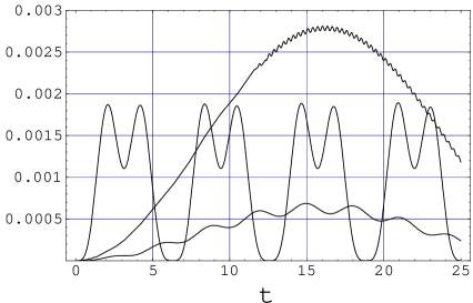
Figure 1: The occupation number of neutrino pairs, ${\mathcal{N}}_{{k},+}^{P}$, as a function of time, for $j^{0}=1+0.1\sin(\omega t)$ and $\vec{j}=0$, all in units of $m$. The upper curve corresponds to $(\omega,k)=(10,4.3)$ (close to resonance), the middle curve to $(1,-0.5)$, and the lower curve to $(0.1,-0.5)$.

The initial state is specified at $t\leq 0$, when the density is time-independent: $\dot{\rho}_{\pm}(t\leq 0)=0$. In a constant density background, the mode functions are plane waves, and we can choose the following initial conditions:

$$f_{k,\pm}^{(\lambda)}(0)=1,\qquad\dot{f}_{k,\pm}^{(\lambda)}(0)=-iE_{k,\pm}^{(\lambda)}(0).$$ (15)

Here

$$E_{k,\pm}^{(\lambda)}(0)=-\frac{1}{2}\rho_{\pm}(0)+\lambda\sqrt{m^{2}+\left(\frac{1}{2}\rho_{\pm}(0)\pm k\right)^{2}}.$$ (16)

are the eigenvalues of the Hamiltonian in matter with a constant density. In the limit $\rho\to 0$, the spinors $U$ and $V$ become the usual free field positive and negative frequency solutions. We normalize the spinors

$$U_{{k},r}^{{\dagger}}(0)U_{{k},s}(0)=V_{-{k},r}^{{\dagger}}(0)V_{-{k},s}(0)=\delta_{rs}.$$ (17)

Due to initial conditions, the orthogonality relation

$$U_{{k},r}^{{\dagger}}(0)V_{-{k},s}(0)=0$$ (18)

is satisfied automatically. Since the time evolution is induced by a hermitian Hamiltonian, the normalization and orthogonality properties of the spinors are preserved. Condition (17) fixes the normalization constants:

$$\left(N_{{k},\pm}^{(\lambda)}\right)^{-2}=\left(E^{(-1)}_{k,\pm}(0)\mp k\right)^{2}+m^{2}.$$ (19)

To simplify notation we will drop the $\lambda$ label from the normalization constants, which are equal for $\lambda=\pm 1$.

The particle number $n_{k,s}(t)=\langle b^{{\dagger}}_{k,s}(t)b_{k,s}(t)\rangle$ is defined in terms of creation and annihilation operators. However, when $b^{{\dagger}}_{k,s}$ and $b_{k,s}$ are time-dependent, the Hamiltonian does not, in general, remain diagonal at all times. This is a sign of particle production. To determine the number of particles, one has to diagonalize the Hamiltonian by a Bogoliubov transformation or, equivalently, project the states at time $t$ from the basis of mode functions $f(t)$ to that of plain waves. A detailed discussion and various applications of this standard technique can be found in Refs. book ; grib ; baa ; gk .

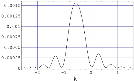
Figure 2: The number density of produced neutrino pairs, ${\mathcal{N}}_{{k},+}^{P}$, as a function of $k$ at $t=10$. The parameters chosen for this plot are $j^{0}=1+0.1\sin(\omega t)$, $\vec{j}=0$, and $\omega=1$, all in units of $m$.

We define the particle number in the basis of plain wave states in the background of constant density $\rho_{\pm}=\rho_{\pm}(0)$. The positive and negative energy modes are given by eqs. (4,5,11) with energies (16) and normalization (19). In this basis the time-dependent particle number is

$${\mathcal{N}}^{P}_{k,s}(t)=|D^{P}_{k,s}|^{2},$$ (20)

where $D^{P}_{k,s}$ is the corresponding Bogoliubov coefficient:

$$D^{P}_{k,\pm}= {U_{{\bf k},\pm}}^{{\dagger}}(0)V_{-{\bf k},\pm}(t)$$ (21)

$$= {m}{N_{{\bf k},\pm}^{2}}\left(i\dot{f}^{(-1)}_{k,s}(t)-f^{(-1)}_{k,s}(t)E^{(-1)}_{k,\pm}(0)\right).$$

Therefore, the particle number is

$${\mathcal{N}}^{P}_{k,\pm}(t)= \frac{m^{2}}{\left[(E_{k,\pm}^{(-1)}(0)\mp k)^{2}+m^{2}\right]^{2}}\times$$ (22)

$$\left\{|\dot{f}^{(-1)}_{k,\pm}(t)|^{2}+|E^{(-1)}_{k,\pm}(0)f^{(-1)}_{k,\pm}(t)|^{2}-\right.$$

$$\left.2E^{(-1)}_{k,\pm}(0){\rm Im}(f^{(-1)}_{k,\pm}(t)\dot{f}^{(-1)*}_{k,\pm}(t))\right\}.$$

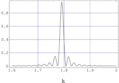
Figure 3: The occupation number for neutrino pairs, ${\mathcal{N}}_{{k},+}^{P}$, as a function of $k$ at $t=175$. The parameters are $j^{\mu}=1+0.1\sin(\omega t)$, $\vec{j}=0$ and $\omega=5$, all in units of $m$. The modes around $k\approx 1.79$ are in resonance.

In all formulas the neutrino momentum only enters in the combination $k_{{\rm eff},\pm}(t)=k\pm\rho_{\pm}(t)/2$. The momentum is shifted due to the effective potential generated by the matter background.

The number of particles at $t=0$ is equal to zero due to the initial conditions (15) and (16). Furthermore, equation (14) implies that at all times the number of particles ${\mathcal{N}}^{P}_{k,s}(t)$ is equal the number of antiparticles, ${\mathcal{N}}^{AP}_{-k}(t)=|D^{AP}_{-k}|^{2}=|{V_{-{k},\pm}}^{{\dagger}}(0)U_{{k},\pm}(t)|^{2}$, as it should be. The total number density of neutrinos pairs is

$$n_{\nu}(t)=\sum_{s=\pm}\int\frac{{\rm d}^{3}k}{(2\pi)^{3}}{\mathcal{N}}^{P}_{k,s}(t).$$ (23)

In the limit of an infinite volume the net amount of neutrinos produced is $n_{\nu}(t_{\rm end})-n_{\nu}(t_{0})$, which goes to zero if the matter density returns to its original state. However, in reality the matter with time-dependent density occupies a finite volume, so that neutrinos can also diffuse away from the production region and break the coherence that was implicitly assumed in derivation of eq. (22). If the diffusion is fast, the density of neutrinos is smaller than the maximal equilibrium value (22) and is nearly constant. In this regime, one can define a particle production rate $\dot{n}_{\nu}(t)$ book .

Particle production vanishes in the limit of a massless neutrino, see eq. (22). This is easy to understand in the current formalism. In the massless limit the right and left handed neutrino sectors decouple, and if the Hamiltonian is diagonal at the initial time it remains so at all times. The Boguliubov transformation is trivial, and, hence, no particle production occurs. This is a consequence of the perturbation $\delta\rho(t)$ being spatially homogeneous. The neutrinos are produced in pairs, and the two neutrinos have opposite momenta in the center of mass frame. Thus, the matrix elements of the form $\langle\bar{\nu}_{\!-\vec{k}}\Gamma^{\mu}\nu_{\vec{k}}\rangle$, where $\Gamma^{\mu}=\gamma^{\mu},\gamma^{\mu}\gamma^{5}$, vanish for massless neutrinos. Spatial perturbations $\delta\rho(\vec{x},t)$ lead to a particle production only if they are time-dependent in all Lorentz frames. For example, for a plane wave perturbation $\delta\rho\propto\cos(\vec{k}\cdot\vec{x}-\omega t)$ one can always make a Lorentz transformation such that $\delta\rho^{\prime}\propto\cos(\vec{k^{\prime}}\cdot\vec{x})$, and particle number remains constant in time. Here the phonons are virtual, and pair production is only possible if additional energy is pumped in the system, as is done in the production mechanism described in loeb . S Using the mode equations (13), we can compute the first and second derivatives of ${\mathcal{N}}^{P}_{k,\pm}$ at $t=0^{+}$. Let us consider time evolution of a two-component vector ${\mathcal{F}}=\{f^{(-1)}_{k,\pm}(t),\dot{f}^{(-1)}_{k,\pm}\}$. One can rewrite the mode equation as

$$\frac{d}{dt}{\mathcal{F}}=S{\mathcal{F}},$$ (24)

where $S$ is a 2$\times$2 matrix:

$$S=\left(\matrix{0&1\cr-(k^{2}\pm k\rho_{\pm}+m^{2})&i\rho_{\pm}(t)}\right).$$ (25)

The expression (22) can also be rewritten as

$${\mathcal{N}}^{P}_{k,\pm}(t)=m^{2}N_{{k},\pm}^{4}{\mathcal{F}}^{{\dagger}}(t)T{\mathcal{F}}(t),$$ (26)

where

$$T=\left(\matrix{|E^{(-1)}_{k,\pm}(0)|^{2}&iE^{(-1)}_{k,\pm}(0)\cr-iE^{(-1)}_{k,\pm}(0)&1}\right).$$ (27)

Now we differentiate eq. (26) and use the identity $T{\mathcal{F}}(0)=0$:

$$\dot{\mathcal{N}}^{P}(0) = m^{2}N_{{k},\pm}^{4}{\mathcal{F}}^{{\dagger}}(0)(S^{{\dagger}}T+TS){\mathcal{F}}(0)=0;$$

$$\ddot{\mathcal{N}}^{P}(0) = m^{2}N_{{k},\pm}^{4}{\mathcal{F}}^{{\dagger}}(0)[S^{{\dagger}}(S^{{\dagger}}T+TS)+$$ (28)

$$(S^{{\dagger}}T+TS)S+(\dot{S}^{{\dagger}}T+T\dot{S})]{\mathcal{F}}(0)$$

$$= 2m^{2}N_{{k},\pm}^{4}\ {\mathcal{F}}^{{\dagger}}(0)S^{{\dagger}}TS{\mathcal{F}}(0).$$

Finally,

$$\dot{\mathcal{N}}^{P}_{k,\pm}(0)=0;\ \ \ddot{\mathcal{N}}^{P}_{k,\pm}(0)=\frac{1}{2}m^{2}N_{{k},\pm}^{4}\dot{\rho}_{\pm}^{2}(0).$$ (29)

Let us now consider a spatially uniform matter density that is changing periodically with time:

$$j_{\mu}(t)=\rho(t)v_{\mu},\ v_{\mu}={\rm const}.$$ (30)

Figures 1-3 show the numerical solutions for the case $j^{0}/m=1+0.1\sin(\omega t)$, $\vec{j}=0$ and various values of $(\omega,k)$. The occupation number density (22) is a periodic function of time, as shown in Fig. 1. This means that neutrinos are created and absorbed through non-perturbative interactions with matter (cf. Ref. book ). At all times ${\mathcal{N}}^{P}_{k,\pm}(t)$ remains smaller than 1, in accordance with the Pauli exclusion principle. The neutrino pair-production occurs in a spectral band centered around $k_{\rm eff}(t_{0})=k\pm\rho_{\pm}(t_{0})/2=0$, as shown in Fig. 2. The value $k_{\rm eff}(t_{0})=0$ minimizes the real part of the frequency in eq. (13). In the adiabatic regime, where $\dot{\rho}\ll k_{\rm eff}^{2}+m^{2}$, the width of the resonance peak is $\Gamma\sim m$. This clearly shows the non-perturbative nature of neutrino pair production in a coherent background. A perturbative calculation involving multiple phonons, each decaying into a neutrino pair, would predict a peak in the spectrum around $k_{\rm eff}\sim\omega/2$ with width $\Gamma\sim G_{\rm F}^{2}\omega^{3}$ for $\omega>m$.

For oscillations with $\rho(t)=\rho_{0}+\delta\rho\sin(\omega t)$, $\delta\rho\ll\rho_{0}$, equation (13) is a (complex) Mathieu equation with purely imaginary parameter $q=i\delta\rho/\omega$ and the $A$-parameter that is also time dependent: $A(k,t)=4(m^{2}+(\rho_{\pm}(t)/2\pm k)^{2})/\omega^{2}$. Strictly speaking, this time dependence makes equation (13) different from the usual Mathieu equation, but the general behavior of its solutions is the same for $\delta\rho\ll\rho$. Since the $q$-parameter is purely imaginary, all solutions are semi-periodic. There are several resonances, the first (and the widest) of which occurs when $A=1$, that is when the frequency and the momentum are related by $4\omega^{2}\approx m^{2}+(k\pm\rho_{0}/2)^{2}$. Fig. 3 shows this resonance for $\omega^{\rm res}=5m$, at time $t=175m^{-1}$. The occupation number ${\mathcal{N}}^{P}_{k,\pm}$ grows for those modes that are in resonance.

There are additional resonant bands for higher values of $A$, that is for smaller oscillation frequencies. However, since the ratio $q/A\propto\omega$ decreases with $\omega$, the higher resonances have diminishing width. Dense stars and other astrophysical objects are generally characterized by small frequencies, so that neutrino production occurs off-resonance.

The parameters in Fig. 1-3 were chosen so as to illustrate the general behavior of the solutions. We now examine the realistic values of these parameters in the neutron stars.

Unless the lightest neutrino is much lighter than the $0.1$ eV scale inferred from the mass-squared difference measured by Super-Kamiokande, the basic oscillation frequencies in neutron stars have $\omega\ll m$, very far from the lowest - and widest - resonance. Of course, higher modes of oscillation may be excited, but they are usually associated with significant dissipation. Let us consider the efficiency of neutrino production for $\rho(t)=\rho_{0}+\delta\rho\sin(\omega t)$ with a small driving frequency $\omega\ll m$. Based on expansions of the Bogoliubov coefficients in eqs. (21,22), we estimate that the neutrino energy production per unit volume is $\dot{\epsilon}\sim m^{2}\max[m^{2},(\delta\rho)^{2}]\omega$. For a realistic case $m\sim\delta\rho\sim 0.1$eV, one can estimate the neutrino production rate in a neutron star with radius $R\approx 10$ km for the basic oscillation frequency $\omega\sim 2\pi c/R$:

$$\dot{E}\sim 10^{22}\left(\frac{m}{0.1{\rm eV}}\right)^{2}\left(\frac{\max[m,\delta\rho]}{0.1{\rm eV}}\right)^{2}{\rm erg\ s}^{-1}$$ (31)

This corresponds to emission of $10^{34}$ low-energy (sub-eV) neutrinos per second. For smaller amplitudes or larger frequencies, the production rates decrease or increase, respectively.

This effect is, clearly, negligible when compared to the energy scale of a supernova explosion. However, it is conceivable that future observations of neutron stars may reveal subtle changes of the rotation speeds of cold oscillating neutron stars that can be compared with our predictions. Neutrino production through the same mechanism can also occur in a neutron star binary system. In the latter case pair-production occurs because the centripetal acceleration $a=\dot{\vec{v}}\neq 0$, and the current $j_{\mu}(t)$ has a non-zero derivative.

In summary, we have described pair creation of neutrinos in a background with time-dependent matter density.

We thank N. Graham, Y. Levin, and R. Peccei for very helpful discussions. This work was supported in part by the US Department of Energy grant DE-FG03-91ER40662, Task C, as well as by a Faculty Grant from UCLA Council on Research.

References

• (1) A. A. Grib, S. G. Mamayev, and V. M. Mostepanenko, Vacuum Quantum Effects in Strong Fields, Friedmann Laboratory Publishing, St. Petersburg, 1994.
• (2) A. A. Grib, V. M. Mostepanenko, and V. M. Frolov, Theor. Math. Phys. 13, 1207 (1972).
• (3) J. M. Cornwall and G. Tiktopoulos, Phys. Rev. D 39, 334 (1989).
• (4) J. Baacke, K. Heitmann and C. Patzold, Phys. Rev. D 58, 125013 (1998).
• (5) P. B. Greene and L. Kofman, Phys. Lett. B 448, 6 (1999); Phys. Rev. D 62, 123516 (2000).
• (6) A. Loeb, Phys. Rev. Lett. 64, 115 (1990) [Erratum-ibid. 64, 3203 (1990)].
• (7) For a recent review of neutrino masses, see, e.g., R. D. Peccei, hep-ph/9906509; Y. Farzan, O. L. Peres and A. Y. Smirnov, hep-ph/0105105.