Scaling property and peculiar velocity of global monopoles

Abstract

We investigate the scaling property of global monopoles in the expanding universe. By directly solving the equations of motion for scalar fields, we follow the time development of the number density of global monopoles in the radiation dominated (RD) universe and the matter dominated (MD) universe. It is confirmed that the global monopole network relaxes into the scaling regime and the number per hubble volume is a constant irrespective of the cosmic time. The number density $n(t)$ of global monopoles is given by $n(t)\simeq(0.43\pm 0.07)/t^{3}$ during the RD era and $n(t)\simeq(0.25\pm 0.05)/t^{3}$ during the MD era. We also examine the peculiar velocity $v$ of global monopoles. For this purpose, we establish a method to measure the peculiar velocity by use of only the local quantities of the scalar fields. It is found that $v\sim(1.0\pm 0.3)$ during the RD era and $v\sim(0.8\pm 0.3)$ during the MD era. By use of it, a more accurate analytic estimate for the number density of global monopoles is obtained.

I Introduction

The grand unified theory based on a simple group predicts magnetic (gauge) monopoles if it breaks to leave the $U(1)$ symmetry of the electromagnetism [2]. Magnetic monopoles are dangerous because they may overclose our universe [2]. However, no magnetic monopoles have been found yet. In fact, the flux of magnetic monopoles is severely constrained by cosmological and astrophysical considerations [3]. Thus, magnetic monopoles produced in the early universe must be diluted away, annihilated, or swept away (the monopole problem). This monopole problem is one of the motivations of inflation [4] though other solutions are also proposed [5, 6].

On the other hand, global monopoles have drawn less attention. However, while magnetic monopoles are dangerous for the cosmic history, global monopoles may be favorable because they may produce primordial density fluctuations responsible for the large scale structure formation and the anisotropy of the cosmic microwave background radiation (CMB) [7, 8, 9, 10, 11]. Recent observations of the CMB by the Boomerang [12] and the MAXIMA [13] experiments found the first acoustic peak with a spherical harmonic multipole $l\sim 200$ predicted by the standard inflationary scenario. But, they also found a relatively low second peak, which may suggest the contribution of topological defects [14]. Moreover, deviations from Gaussianity in CMB are reported in [15]. Thus, though it is improbable for topological defects to become the primary source of primordial density fluctuations, a hybrid model is still attractive, where primordial density fluctuations are comprised of adiabatic fluctuations induced by inflation and isocurvature ones induced by topological defects. In fact, topological defects can be easily compatible with inflation [16, 17, 18].

The key property of global monopoles to contribute primordial density fluctuations properly is scaling, where the typical scale of the global monopole network grows in proportion to the horizon scale. Then the number density of global monopoles is proportional to $t^{-3}$ ($t$ : the cosmic time). Here we define the scaling parameter $\xi$ as

$$\xi\equiv n(t)t^{3},$$ (1)

where $n(t)$ is the number density of global monopoles. If $\xi$ becomes a constant irrespective of the cosmic time, we can conclude that the global monopole network goes into the scaling regime.

The mass of a global monopole $m$ is proportional to the distance to the nearest neighborhood antimonopole $d$ [$m\simeq 4\pi\eta^{2}d$, $\eta$ : the absolute magnitude of vacuum expectation values (VEV) of scalar fields]. Roughly speaking, the distance is the horizon scale (to be exact $d\simeq t/\xi^{1/3}$ ) if the network follows the scaling property. Then the density fluctuations produced by global monopoles are given by

$$\frac{\delta\rho}{\rho} \simeq mn~{}8\pi/3m_{\rm pl}^{2}H^{2}$$ (2)

$$\simeq \frac{128}{3}~{}(24)~{}\pi^{2}\xi^{2/3}\left(\frac{\eta}{m_{\rm pl}}\right)^{2}\qquad{\rm for~{}RD~{}(MD)},$$ (3)

where $m_{\rm pl}=1.2\times 10^{19}$ GeV is the Plank mass. Thus, the density fluctuations produced by global monopoles become scale invariant. One may wonder if the precise value of $\xi$ is not so important because the amplitude of density fluctuations depends on only the combination of $\xi^{2/3}\eta^{2}$. It is true for the case where global monopoles are the dominant source of density fluctuations. But that is not the case. As stated earlier, the recent observations indicate that the dominant source of density fluctuations is inflation and topological defects contribute to them subdominantly. In such a case, $\xi$ itself determines the ratio of the above two contributions for a fixed VEV. Thus, the precise value of $\xi$ is increasingly important.

The cosmological evolution of global monopoles was first discussed by Barriola and Vilenkin [7]. They showed that the annihilation is so efficient that global monopoles do not overclose our universe unlike magnetic monopoles, but that it is not too efficient to survive in our universe. This is mainly because an attractive force works between a monopole and an antimonopole. Then, Bennett and Rhie performed the first numerical simulations and found the tendency that the number of global monopoles per horizon volume is nearly a constant [8]. However they used the nonlinear $\sigma$ model approximation as equations of motion to evolve the scalar fields. Later, Pen, Spergel, and Turok made numerical simulations in both the nonlinear $\sigma$ model approximation and the full potential [10]. (See also [11].) However, due to the lack of the computer power, they can run a few realizations so that the scaling property cannot be confirmed definitely. Many realizations of numerical simulations are needed to decrease the error and estimate it statistically. Furthermore, in order to confirm the scaling property completely, we should pay attention to several effects, which may affect the final result, for example, the boundary effect, the grid size effect, the total box size dependence, and so on.

In the previous paper [22], we reported the results of our numerical simulations of the global monopole network and confirmed that the global monopole network relaxes into the scaling regime both in the RD and the MD universe. In this paper, we investigate the cosmological evolution of the global monopole network comprehensively.

In the next section, we give the formulation and the results of our numerical simulations. From the symmetry restoration phase, we follow the evolution of the scalar fields with the $O(3)$ symmetry, which breaks to generate global monopoles. The time development of the number density of global monopoles is examined. Since we need to perform a lot of realizations, it is important to establish the method to identify monopoles automatically from the values of the scalar fields. We will propose two identification methods and compare the results obtained by both methods. We also investigate the peculiar velocity of global monopoles. Our numerical simulations are based on the Eulerian view. Therefore, it is very difficult to know where a monopole moves after the long interval enough to measure the velocity. We establish the method to measure the velocity of global monopoles by use of only the local quantities of scalar fields. In Sec. III, we set up the Boltzmann equation for the time development of the number density of global monopoles. Using the peculiar velocity obtained from numerical simulations, an analytic estimate for the number density of global monopoles is given. In the final section, we give the summary.

II Numerical Simulations

First of all, we give the formalism of our numerical simulations to follow the evolution of the global monopole network. Later we show the results of our numerical simulations and discuss whether the global monopole network goes into the scaling regime. Furthermore, the peculiar velocity of global monopoles is investigated.

We directly solve the equations of motion for scalar fields in the expanding universe, which have the $O(3)$ symmetry at high temperature and later break to generate global monopoles. We consider the following Lagrangian density for scalar fields $\phi^{a}(x)(a=1,2,3)$:

$${\cal L}[\phi^{a}]=\frac{1}{2}g_{\mu\nu}\partial^{\mu}\phi^{a}\partial^{\nu}\phi^{a}-V_{\rm eff}[\phi^{a},T].$$ (4)

Here $g_{\mu\nu}$ is the flat Robertson-Walker metric and the effective potential $V_{\rm eff}[\phi^{a},T]$, which represents the typical second order phase transition, is given by

$$V_{\rm eff}[\phi^{a},T] = \frac{\lambda}{4}(\phi^{2}-\sigma^{2})^{2}+\frac{5}{24}\lambda T^{2}\phi^{2},$$ (5)

$$= \frac{\lambda}{4}(\phi^{2}-\eta^{2})^{2}+\frac{\lambda}{4}(\sigma^{4}-\eta^{4}),$$ (6)

where $\phi\equiv\sqrt{\phi^{a}\phi^{a}}$, $\eta\equiv\sigma\sqrt{1-(T/T_{c})^{2}}$ and $T_{c}\equiv\frac{2}{5}\sqrt{15}\sigma$ is the critical temperature. For $T>T_{c}$, the potential $V_{\rm eff}[\phi^{a},T]$ has a minimum at the origin and the $O(3)$ symmetry is restored. On the other hand, for $T<T_{c}$, new minima $\phi=\eta$ appear and the symmetry is broken, which leads to the formation of global monopoles.

The equations of motion for the scalar fields $\phi^{a}$ in the expanding universe are given by

$$\ddot{\phi^{a}}(x)+3H\dot{\phi^{a}}(x)-\frac{1}{R(t)^{2}}\nabla^{2}\phi^{a}(x)+\lambda\left(\phi^{2}(x)-\eta^{2}\right)\phi^{a}(x)=0,$$ (7)

where the dot represents the time derivative and $R(t)$ is the cosmic scale factor. The Hubble parameter $H=\dot{R}(t)/R(t)$ and the cosmic time $t$ are given by

$$H^{2} = \frac{4\pi^{3}}{45m_{\rm pl}^{2}}g_{*}T^{4},~{}~{}~{}t=\frac{1}{2H}\equiv\frac{\epsilon_{RD}}{T^{2}}~{}~{}~{}~{}~{}~{}~{}~{}({\rm for~{}RD}),$$ (8)

$$H^{2} = \alpha(T)\frac{4\pi^{3}}{45m_{\rm pl}^{2}}g_{*}T^{4},~{}~{}t=\frac{2}{3H}\equiv\frac{\epsilon_{MD}}{T^{3/2}}~{}~{}({\rm for~{}MD}),$$ (9)

with $g_{*}$ to be the total number of degrees of freedom for the relativistic particles. For the MD case, we have defined $\alpha(T)$ [$\alpha(T)>1$] as $\alpha(T)\equiv\rho_{\rm mat}(T)/\rho_{\rm rad}(T)=\alpha_{c}(T_{c}/T)$, where $\rho_{\rm mat}(T)$ is the contribution to the energy density from nonrelativistic particles, $\rho_{\rm rad}(T)$ is the contribution from relativistic particles at the temperature $T$, and $\alpha_{c}\equiv\rho_{\rm mat}(T_{c})/\rho_{\rm rad}(T_{c})$. We also define the dimensionless parameter $\zeta$ as

$$\zeta_{RD} \equiv \frac{\epsilon_{RD}}{\sigma}=\left(\frac{45}{16\pi^{3}g_{*}}\right)^{1/2}\frac{m_{\rm pl}}{\sigma}~{}~{}~{}~{}~{}~{}~{}({\rm for~{}RD}),$$ (10)

$$\zeta_{MD} \equiv \frac{\epsilon_{MD}}{\sigma^{1/2}}=\left(\frac{5\sqrt{15}}{6\alpha_{c}\pi^{3}g_{*}}\right)^{1/2}\frac{m_{\rm pl}}{\sigma}~{}~{}~{}~{}({\rm for~{}MD}).$$ (11)

In our simulation, we take $\zeta_{RD,MD}=10$ and $5$ to investigate the $\zeta$ dependence on the result.

We start the numerical simulations from the $O(3)$ symmetric phase with the temperature $T_{i}=2T_{c}$, which corresponds to $t_{i}=t_{c}/4$(RD) and $t_{i}=t_{c}/(2\sqrt{2})$(MD). At the initial time ($t_{i}<t_{c}$), we adopt as the initial condition the thermal equilibrium state with the mass

$$m=\sqrt{\frac{5}{12}\lambda(T_{i}^{2}-T_{c}^{2})},$$ (12)

which is the inverse curvature of the potential at the origin at $t=t_{i}$.

Hereafter we normalize the scalar field in units of $t_{i}^{-1}$, $t$ and $x$ in units of $t_{i}$. We set $\lambda$ to be $\lambda=0.25$ and normalize the scale factor $R(t)$ as $R(1)=1$. Then, the normalized equations of motion for the scalar fields $\phi^{a}$ are given by

$$\ddot{\phi^{a}}(x)+\frac{3}{2t}\dot{\phi^{a}}(x)-\frac{1}{t}\nabla^{2}\phi^{a}(x)+\lambda(\phi^{2}-\eta_{RD}^{2})\phi^{a}=0\hskip 56.9055pt({\rm for~{}RD}),$$ (13)

$$\ddot{\phi^{a}}(x)+\frac{2}{t}\dot{\phi^{a}}(x)-\frac{1}{t^{4/3}}\nabla^{2}\phi^{a}(x)+\lambda(\phi^{2}-\eta_{MD}^{2})\phi^{a}=0\hskip 45.52458pt({\rm for~{}MD})$$ (14)

with $\eta_{RD}=\frac{5}{48}\zeta_{RD}\sqrt{1-4/t}$ and $\eta_{MD}=(\sqrt{15}/12)^{3/2}\zeta_{MD}\sqrt{1-4/t^{4/3}}$.

We perform numerical simulations in seven different sets of lattice sizes and lattice spacings in the RD universe and the MD universe (See Tables I and II.). In all cases, the time step is taken to be $\delta t=0.01$. In the typical case (1), the box size is nearly equal to the horizon volume $(H^{-1})^{3}$ and the lattice spacing to the typical core size of a monopole $\delta x\sim 1.0/(\sqrt{\lambda}\sigma)$ at the final time $t_{f}$. Furthermore, in order to investigate the dependence of $\zeta$, we arrange the case (7) with $\zeta=5$. We have simulated the system from 10 [(2), (3), (5) and (6)] or 50 [(1), (4), and (7)] different thermal initial conditions. Also, in order to investigate the effect of the boundary condition (BC), we adopt both the periodic BC and the reflective BC [$\nabla^{2}\phi^{a}(x)=0$ on the boundary].

A Number density

In order to judge whether the global monopole network relaxes into the scaling regime, we follow the time development of $\xi$. If $\xi$ becomes a constant irrespective of the cosmic time, we can conclude that the global monopole network goes into the scaling regime.

First of all, we need to count the number of global monopoles in the simulation box. For the purpose, we must establish the identification method of global monopoles because we can obtain only the values of scalar fields. We propose two identification methods and later compare the results obtained by using both methods. In the first method (I), we use a static spherically-symmetric solution with the topological charge $N=1$, which is obtained by solving the equation

$$\frac{d^{2}\phi}{dr^{2}}+\frac{2}{r}\frac{d\phi}{dr}-2\frac{\phi}{r^{2}}-\frac{dV_{\rm eff}[\phi,T]}{d\phi}=0$$ (15)

with $\phi^{a}(r,\theta,\varphi)\equiv\phi(r)x^{a}/r$, $x^{1}=r\sin\theta\cos\varphi,x^{2}=r\sin\theta\sin\varphi$, and $x^{3}=r\cos\theta$. The boundary conditions are given by

$$\phi(r) \rightarrow \eta\qquad(r\rightarrow\infty),$$ (16)

$$\phi(0) = 0.$$ (17)

One should notice that a point with $\phi^{a}=0$ for all $a$’s is not necessarily situated at a lattice point. In the worst case, a point with $\phi^{a}=0$ lies at the center of a cube. Then, we make the criterion that a lattice is identified with a part of a monopole core if the potential energy density there is larger than that corresponding to the field value of a static spherically-symmetric solution at $r=\sqrt{3}\delta x_{\rm{phys}}/2$ [$\delta x_{\rm{phys}}=R(t)\delta x$], that is, the potential energy density at the vertices when a static spherically-symmetric monopole lies at the center of cube. Moreover, in order to reduce the error, we look on the identified lattices which are connected as one monopole core. In the other method (II), a cubic box is regarded as including a monopole if all $\phi^{a}=0$ ($a$ = 1, 2, 3) surfaces pass through the cubic box, that is, the signs of all eight vertices of the box are not identical for each three field $\phi^{a}$. In this method, we also look on the identified boxes which are connected as one monopole core. In fact, as shown later, the results with these two identification methods coincide very well.

First of all, we discuss the evolution of global monopoles in the RD universe. The time development of $\xi_{RD}$ in the cases from (1) to (6) under the periodic BC is described in Figs. 1. Asterisks ($\ast$) represent the time development of $\xi_{RD}$ for the identification method (I). Squares ($\Box$) represent the time development of $\xi_{RD}$ for the identification method (II). As easily seen, the results with two identification methods coincide very well. We also find that after some relaxation period, $\xi_{RD}$ becomes a constant irrespective of time for all cases. Though all results are consistent within the standard deviation, $\xi_{RD}$ tends to increase as the box size does. This is understood as follows: under the periodic BC, a monopole can annihilate with an antimonopole which lies beyond the boundary. Therefore monopoles under the periodic BC annihilate more often than those in the real universe, in particular, monopoles annihilate more often for smaller box sizes. On the other hand, the time development of $\xi_{RD}$ in the cases from (1) to (6) under the reflective BC is described in Figs. 2. We also find that, $\xi_{RD}$ tends to become a constant though more relaxation period takes. Contrary to the case under the periodic BC, $\xi_{RD}$ tends to decrease as the box size increases. This is understood as follows: under the reflective BC, field configurations of a monopole extend with the same phase direction beyond the boundary so that a monopole cannot annihilate any antimonopoles which may lie beyond the boundary in the real universe. Therefore monopoles under the reflective BC annihilate less often than those in the real universe, in particular, monopoles annihilate less often for smaller box sizes. Thus, $\xi_{RD}$ takes a larger value in a smaller-box simulation due to the boundary effect. After all, the real number of the monopole per the horizon volume lies in between those under the periodic BC and the reflective BC. $\xi_{RD}$ of each case is listed in Table I. From the results of the largest-box simulations [case (6)], we can conclude that the global monopole network relaxes into scaling regime in the RD universe and $\xi_{RD}$ converges to a constant $\xi_{RD}\simeq(0.43\pm 0.07)$. We also show the time development of $\xi_{RD}$ with $\zeta=5$ in the case (7) (Fig. 3). $\xi_{RD}$ asymptotically becomes a constant $\xi_{RD}\simeq(0.36\pm 0.01)$ under the periodic BC, which is consistent with the above all cases with $\zeta=10$ within the standard deviation. Hence we can also conclude that $\zeta$ does not change the essential result.

For the MD case, we also find that after some relaxation period, the number of global monopoles per the horizon volume becomes a constant irrespective of the cosmic time under the periodic BC except for the cases (1), (2), and (3), in which global monopoles annihilate too much due to the boundary effect. Also, the number of global monopoles per the horizon volume becomes a constant irrespective of the cosmic time under the reflective BC except for the case (2), where the boundary effect is the most manifest because of the longest time simulation. The tendency of the boundary effect is the same with that for the RD case. Then, from the results of the largest-box simulations [case (6)], we conclude that the global monopole network relaxes into scaling regime in the MD universe and $\xi_{MD}$ converges to a constant $\xi_{MD}\simeq(0.25\pm 0.05)$ (see Fig. 4 and 5). We also show the time development of $\xi_{MD}$ with $\zeta=5$ in the case (7) (Fig. 6). $\xi_{MD}$ asymptotically becomes a constant $\xi_{MD}\simeq(0.44\pm 0.03)$ under the reflective BC though monopoles tend to disappear under the periodic BC due to the boundary effect. This is consistent with the above all cases with $\zeta=10$ within the standard deviation. Thus, we have completely confirmed that the global monopole network goes into the scaling regime in both the RD universe and MD universe.

B Peculiar velocity

In this subsection, we investigate the peculiar velocity of global monopoles in the expanding universe. In order to measure the peculiar velocity, we need to know where a monopole moves at the next step. For the purpose, we need to find the method to look on the monopole found at each time as the same. But, generally speaking, it is very difficult in case there are a lot of monopoles in the simulation box.

Then, looking at the matter from another angle, we make best use of the information of scalar fields. Since the values and the time derivatives of scalar fields include all informations about monopoles, the velocity of a monopole can be represented by only the information of scalar fields, that is, local quantities. In fact, it is possible as shown below. First of all, we expand scalar fields $\phi^{a}(\mbox{\boldmath${x}$},t)$ around $\phi^{a}(\mbox{\boldmath${x}$}_{0},t_{0})$ up to the first order,

$$\phi^{a}(\mbox{\boldmath${x}$},t)\simeq\phi^{a}(\mbox{\boldmath${x}$}_{0},t_{0})+\nabla\phi^{a}(\mbox{\boldmath${x}$}_{0},t_{0})\cdot(\mbox{\boldmath${x}$}-\mbox{\boldmath${x}$}_{0})+\dot{\phi}^{a}(\mbox{\boldmath${x}$}_{0},t_{0})(t-t_{0})\qquad(a=1,2,3).$$ (18)

The monopole core is identified with the zero of all scalar fields $\phi^{a}$. Assuming a monopole lies at $\mbox{\boldmath${x}$}_{0}$ at the time $t_{0}$, the position ${x}$ of the monopole core at the sufficiently near time $t$ is obtained as the intersection of the following three planes,

$$\mbox{\boldmath${A}$}^{a}\cdot(\mbox{\boldmath${x}$}-\mbox{\boldmath${x}$}_{0})+B^{a}(t-t_{0})=0,$$ (19)

where $\mbox{\boldmath${A}$}^{a}\equiv\nabla\phi^{a}(\mbox{\boldmath${x}$}_{0},t_{0})$ and $B^{a}\equiv\dot{\phi}^{a}(\mbox{\boldmath${x}$}_{0},t_{0})$. These equations are easily solved by the Cramer’s formula

$$\frac{(\mbox{\boldmath${x}$}-\mbox{\boldmath${x}$}_{0})_{j}}{t-t_{o}}=-\frac{\begin{array}[]{ccc}&j&\\ \vline A^{1}_{x}&B^{1}&A^{1}_{z}\vline\\ \vline A^{2}_{x}&B^{2}&A^{2}_{z}\vline\\ \vline A^{3}_{x}&B^{3}&A^{3}_{z}\vline\end{array}}{\begin{array}[]{ccc}\vline A^{1}_{x}&A^{1}_{y}&A^{1}_{z}\vline\\ \vline A^{2}_{x}&A^{2}_{y}&A^{2}_{z}\vline\\ \vline A^{3}_{x}&A^{3}_{y}&A^{3}_{z}\vline\end{array}}~{}.$$ (20)

Thus, the peculiar velocity of a global monopole $v$ can be estimated as

$$v=\frac{|\mbox{\boldmath${x}$}-\mbox{\boldmath${x}$}_{0}|}{t-t_{o}}.$$ (21)

This method has two main sources to generate errors. First of all, our estimate is correct only up to the first order. Then, in order to reduce the error due to this approximation, we evaluate the peculiar velocity for the case (3) in all the situations because it is the simulation with the highest resolution (the smallest lattice spacing). Next, a monopole does not necessarily lie just on the lattice in our simulations. Especially, in the identification method (I), we have identified a lattice with a part of the monopole core if the potential energy at the lattice is larger than a critical value. Since we have started the simulation from the thermal equilibrium states, there are still small thermal fluctuations at late times, which may accidentally lead to the large potential energy for the lattices not corresponding to the monopole core. Thus, in the identification method (I), some lattices which have nothing to do with the monopole core may be identified with monopole cores. At such lattices, the velocities obtained by the above formula may become extraordinarily large, which causes the large error. Then, in order to reduce the errors, we introduce the cutoff for the velocity and abandon the velocities which are larger than a cutoff at estimating the average and dispersion of the velocity. We have chosen several cutoff values and investigated their effects on the results. We found that the results do not change much if the cutoff is smaller than a value (of course, it need to be larger than unity). Though the velocity is at most unity, we set the cutoff to be 1.5 in order to use as many data as possible and reduce the artificial effect.

The time development of the peculiar velocity of global monopoles during the RD era under both the periodic and the reflective BCs is depicted in Fig. 7. Though there is still large uncertainty, the peculiar velocity $v$ takes almost the same constant asymptotically under both BCs and is given by $v_{RD}\sim(1.0\pm 0.3)$. On the other hand, the time development of the peculiar velocity of global monopoles during the MD era is depicted in Fig. 8 and the peculiar velocity $v$ is given by $v_{MD}\sim(0.8\pm 0.3)$. Since monopoles disappear at late times under the periodic BC, the peculiar velocity is set to zero in such a situation.

The obtained values of the peculiar velocity are roughly understood as follows. A constant long-range attractive force works between a monopole and an antimonopole due to the gradient energy of the scalar fields. Then, the monopole is accelerated very much and the relative velocity rapidly gets to the order of unity. In the RD universe, the cosmic expansion is not so rapid that the redshift of the velocity due to the cosmic expansion becomes negligible and the velocity reaches almost the unity. On the other hand, in the MD era, the universe expands so rapid that the velocity is redshifted and it takes a value smaller than the unity.

III Analytic Estimate

In this section, we give a simple analytic estimate for the scaling parameter $\xi$.

The evolution for the number density of global monopoles $n(t)$ can be described by the following Boltzmann equation,

$$\frac{dn(t)}{dt} = -P(t)n(t)-3H(t)n(t),$$ (22)

$$= -\frac{n(t)}{T(t)}-\frac{3mn(t)}{t},$$ (23)

where $R(t)\propto t^{m}$, $P(t)$ is the probability per unit time that a monopole annihilates with an antimonopole, and $T(t)$ is the period it takes for a pair of monopoles at rest with the mean separation $l(t)$ to pair annihilate. The mean separation $l(t)$ is given by $l(t)\equiv R(t)r_{s}=n(t)^{-1/3}$, where $r_{s}$ is the mean comoving separation. In the previous publication [22], we assumed that the relative velocity between them reaches the order of unity at once because a constant attractive force works between a pair of monopoles irrespective of the separation length. In the previous section, we have confirmed that the above assumption is basically correct but the peculiar velocity is smaller than unity in the MD universe. Then, assuming that the relative velocity is given by the peculiar velocity obtained in the previous section and a pair of monopoles does not spiral around each other for a long time, we give a more accurate analytic estimate for the number density of global monopoles. The period $T(t)$ is given by the following relation,

$$v\int^{T+t_{0}}_{t_{0}}\frac{dt}{R(t)}\simeq\int^{r_{s}}_{0}dr,$$ (24)

where $t_{0}$ is the initial time where a pair of monopoles are at rest. Then, the period $T(t)$ reads

$$T(t)\simeq\left(\frac{1-m}{v\,t^{m}n(t)^{1/3}}\right)^{\frac{1}{1-m}}\qquad\qquad({\rm for}~{}~{}t_{0}\ll T).$$ (25)

Inserting this result into the Boltzmann equation (23), the number density $n(t)$ takes the following asymptotic value:

$$n(t)\simeq\frac{\,3^{3\,(1-m)}~{}(1-m)^{\,3\,(2-m)}}{v^{3}t^{3}}\propto t^{-3}.$$ (26)

From the above asymptotic form, first of all, we find that the number density $n(t)$ is proportional to the inverse of the cosmic time cubed, $t^{-3}$, which implies that $\xi$ becomes a constant irrespective of the cosmic time. $\xi$ is also estimated as

$$\xi=\frac{3^{\,3\,(1-m)}~{}(1-m)^{\,3\,(2-m)}}{v^{3}}.$$ (27)

Inserting $m=1/2$ and $v_{RD}\sim(1.0\pm 0.3)$, $\xi_{RD}\sim(0.45\pm 0.22)$. On the other hand, inserting $m=2/3$ and $v_{MD}\sim(0.8\pm 0.3)$, $\xi_{MD}\sim(0.17\pm 0.13)$. Thus, $\xi$ obtained by the analytic estimates can well reproduce that obtained from the numerical simulations both in the RD universe and the MD universe.

IV Summary

In this paper, we have discussed the evolution of the global monopole network in the expanding universe. We have completely confirmed that the global monopole network relaxes into the scaling regime, where the number of global monopoles per the horizon volume is a constant. The scaling parameter $\xi$ is given by $\xi_{RD}\simeq(0.43\pm 0.07)$ in the RD universe and $\xi_{MD}\simeq(0.25\pm 0.05)$ in the MD universe. We also investigated the peculiar velocity of global monopoles. First of all, we established the method to measure the peculiar velocity by using only the local quantities of the scalar fields. This method compensates the weak point of the Eulerian view which our numerical simulations are based on, that is, we cannot follow the motion of each monopole in detail. We find that the peculiar velocity also becomes a constant irrespective of the cosmic time and is given by $v_{RD}\sim(1.0\pm 0.3)$ and $v_{MD}\sim(0.8\pm 0.3)$ though there is still large uncertainty. By use of the Boltzmann equation for the time development of the number density and the peculiar velocity obtained from numerical simulations, we give a simple analytic estimate for the number density, which can well reproduce the results from the numerical simulations up to the proportional coefficient $\xi$.

ACKNOWLEDGMENTS

The author is grateful to J. Yokoyama for useful comments. This work was partially supported by the Japanese Grant-in-Aid for Scientific Research from the Ministry of Education, Culture, Sports, Science, and Technology.

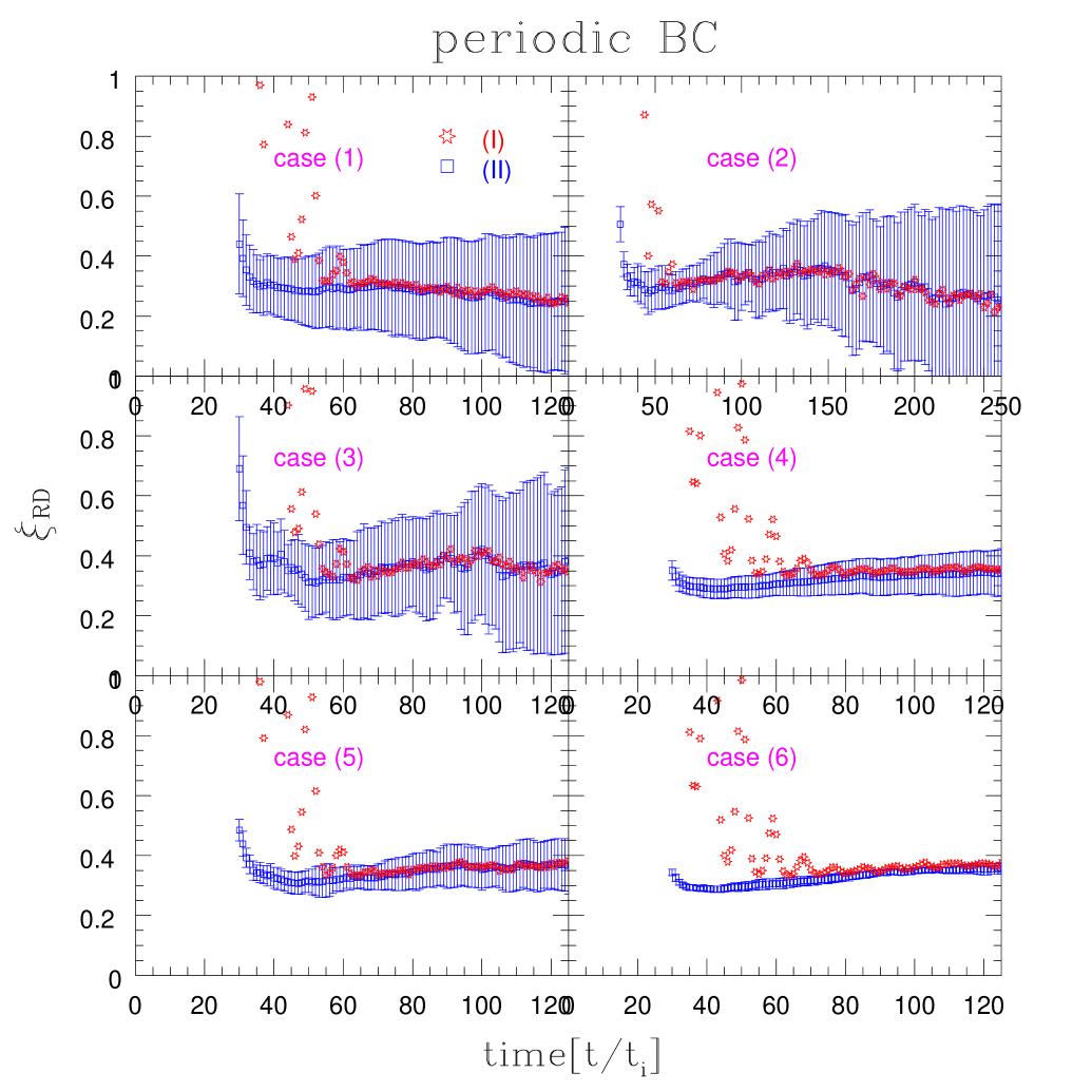
FIG. 1.: The time development of $\xi_{RD}$ in the cases from (1) to (6) under the periodic BC for the RD case. Asterisks ($\ast$) represent time development of $\xi_{RD}$ for the identification method (I). Squares ($\Box$) represent time development of $\xi_{RD}$ for the identification method (II). The vertical lines denote a standard deviation over different initial conditions for the identification method (II).

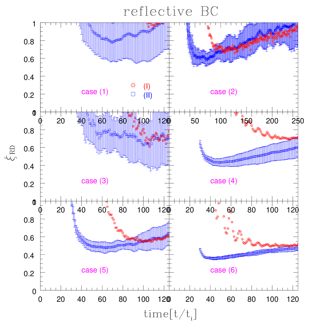
FIG. 2.: That under the reflective BC.

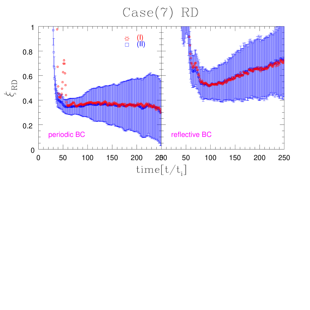
FIG. 3.: The time development of $\xi_{RD}$ in the RD universe for the case (7) under the periodic BC and the reflective BC.

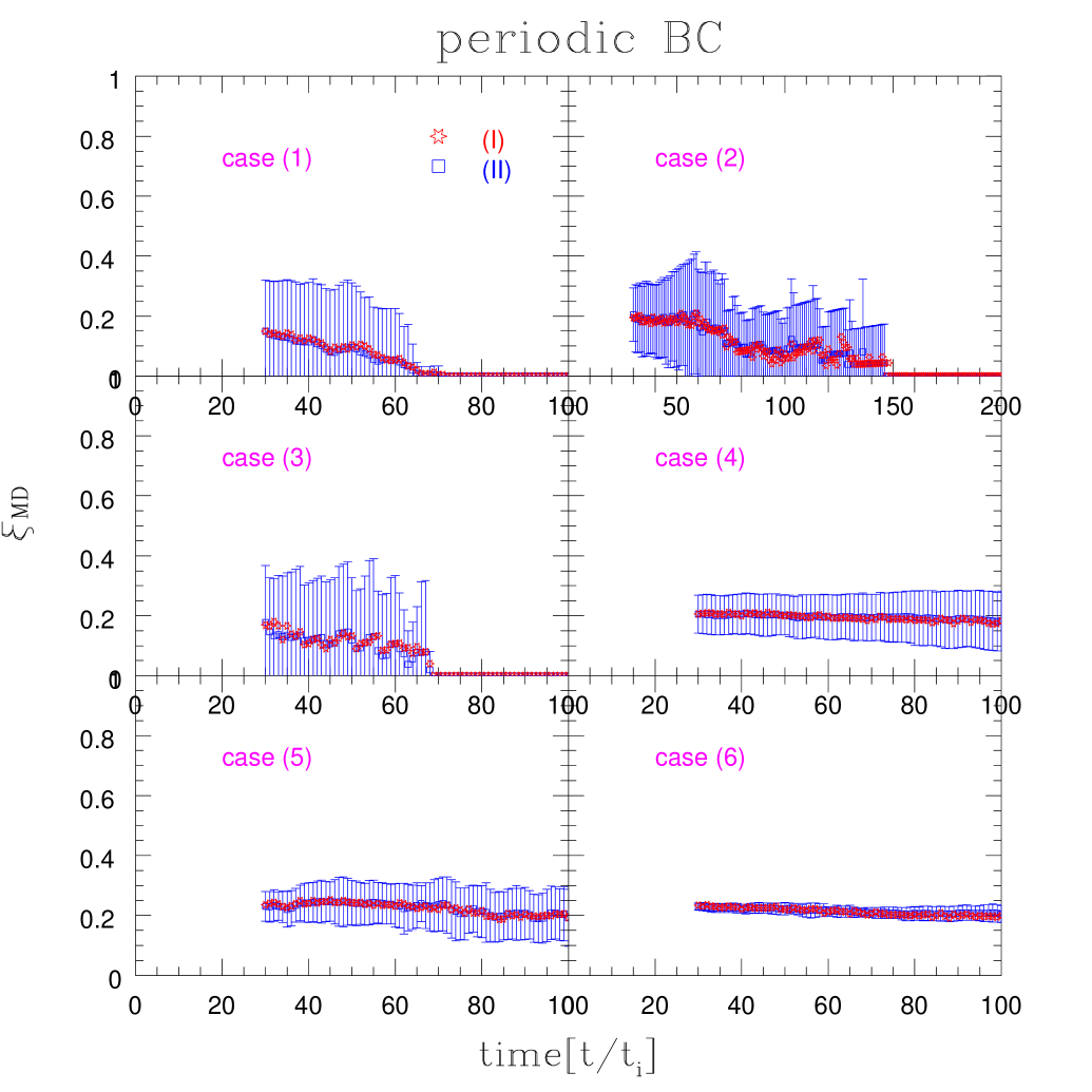
FIG. 4.: The time development of $\xi_{MD}$ in the cases from (1) to (6) under the periodic BC for the MD case. Asterisks ($\ast$) represent time development of $\xi_{MD}$ for the identification method (I). Squares ($\Box$) represent time development of $\xi_{MD}$ for the identification method (II). The vertical lines denote a standard deviation over different initial conditions.

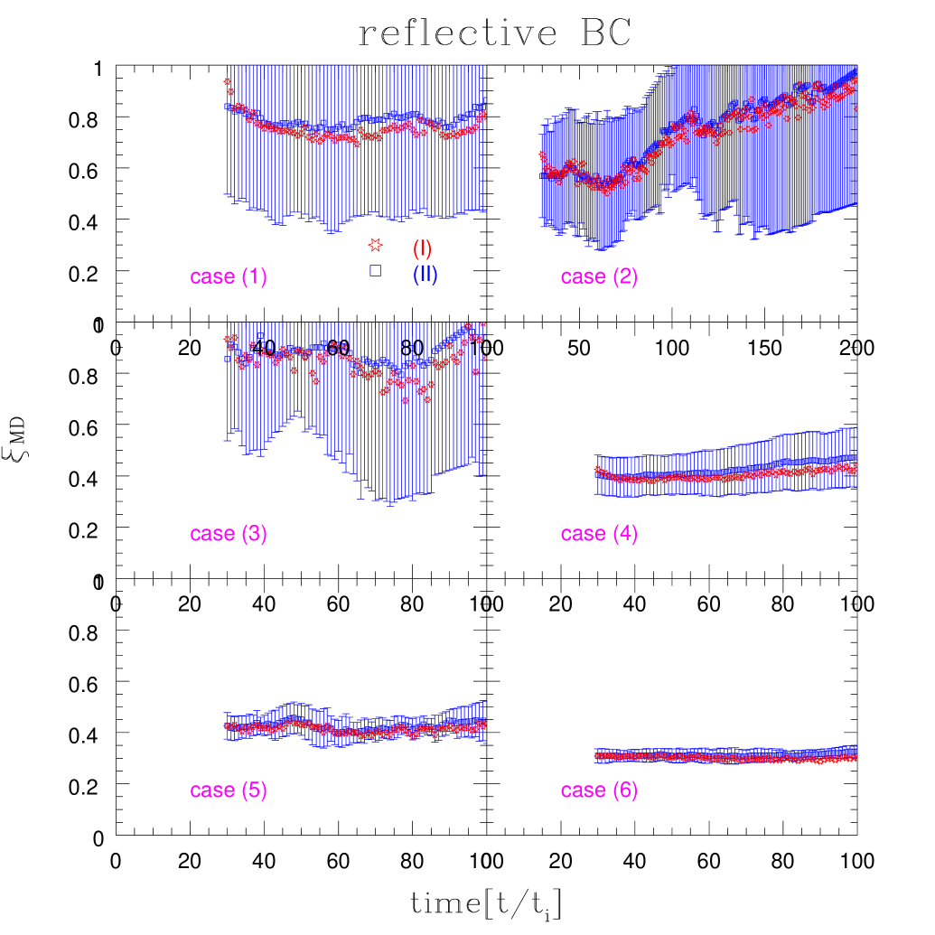
FIG. 5.: That under the reflective BC.

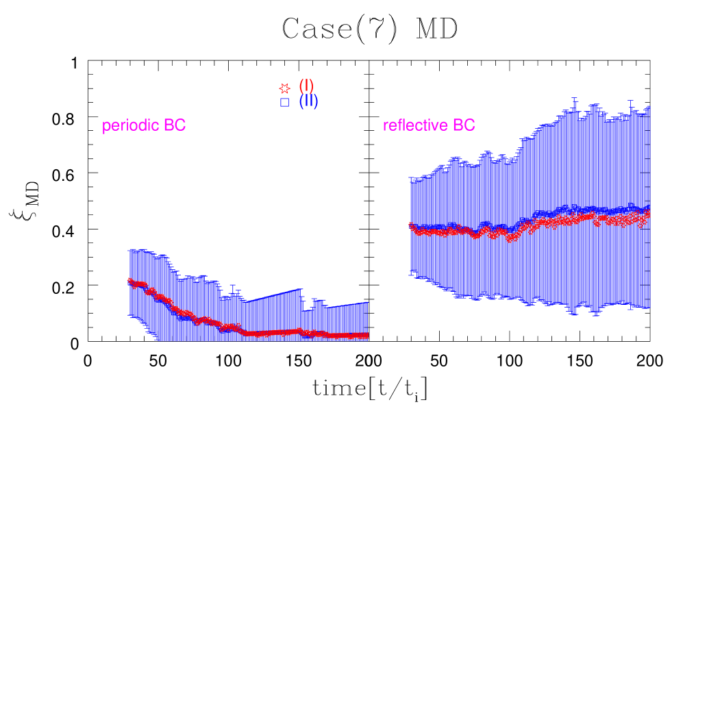
FIG. 6.: The time development of $\xi_{MD}$ in the MD universe for the case (7) under the periodic BC and the reflective BC.

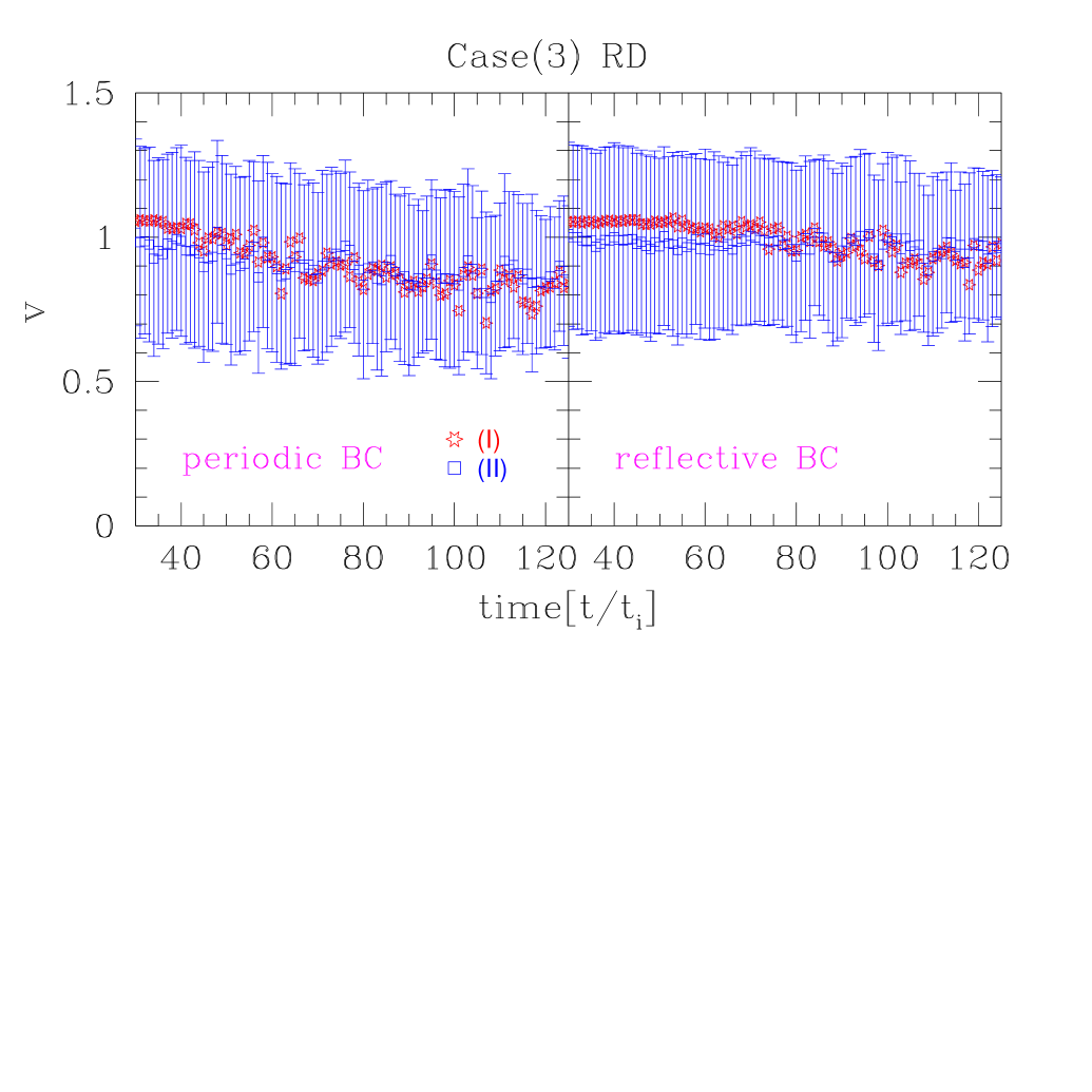
FIG. 7.: The time development of the peculiar velocity in the RD universe for the case (3) under the periodic and the reflective BC. Asterisks ($\ast$) represent time development of the peculiar velocity $v$ for the identification method (I). Squares ($\Box$) represent time development of the peculiar velocity $v$ for the identification method (II). The vertical lines denote a standard deviation over different initial conditions for the identification method (II).

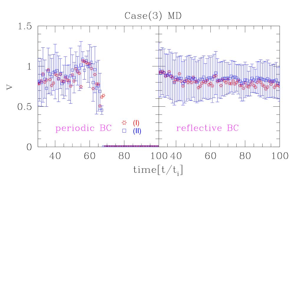
FIG. 8.: The time development of the peculiar velocity in the MD universe for the case (3) under the periodic and the reflective BC. Since monopoles disappear at late times under the periodic BC, the peculiar velocity is set to zero in such a situation.

TABLE I.: Seven different sets of the simulations for the RD case.

Case	Lattice	Lattice spacing ($\delta x$)	$\zeta$	Realization	${\rm Box~{}size}/H^{-1}$	$\xi$	$\xi$
	number	[unit = $t_{i}R(t)$]			(at final time)	(periodic B.C.)	(reflective B.C.)
(1)	$128^{3}$	$\sqrt{3}/10$	10	50	1(at 125)	$0.28\pm 0.19$	$1.00\pm 035$
(2)	$256^{3}$	$\sqrt{6}/20$	10	10	1(at 250)	$0.31\pm 0.20$	$0.83\pm 0.15$
(3)	$256^{3}$	$\sqrt{3}/20$	10	10	1(at 125)	$0.35\pm 0.21$	$0.71\pm 0.33$
(4)	$128^{3}$	$\sqrt{3}/5$	10	50	2(at 125)	$0.37\pm 0.06$	$0.71\pm 0.11$
(5)	$256^{3}$	$\sqrt{3}/10$	10	10	2(at 125)	$0.36\pm 0.07$	$0.58\pm 0.12$
(6)	$256^{3}$	$\sqrt{3}/5$	10	10	4(at 125)	$0.36\pm 0.01$	$0.50\pm 0.03$
(7)	$128^{3}$	$\sqrt{6}/10$	5	50	1(at 250)	$0.36\pm 0.17$	$0.61\pm 0.21$

TABLE II.: Seven different sets of the simulations for the MD case.

Case	Lattice	Lattice spacing ($\delta x$)	$\zeta$	Realization	${\rm Box~{}size}/H^{-1}$	$\xi$	$\xi$
	number	[unit = $t_{i}R(t)$]			(at final time)	(periodic B.C.)	(reflective B.C.)
(1)	$128^{3}$	$3(100)^{1/3}/256$	10	50	1(at 100)	Disappearance	$0.75\pm 0.36$
(2)	$256^{3}$	$3(200)^{1/3}/128$	10	10	1(at 200)	Disappearance	$0.77\pm 0.10$
(3)	$256^{3}$	$3(100)^{1/3}/512$	10	10	1(at 100)	Disappearance	$0.82\pm 0.50$
(4)	$128^{3}$	$3(100)^{1/3}/128$	10	50	2(at 100)	$0.19\pm 0.09$	$0.42\pm 0.10$
(5)	$256^{3}$	$3(100)^{1/3}/256$	10	10	2(at 100)	$0.21\pm 0.09$	$0.41\pm 0.05$
(6)	$256^{3}$	$3(100)^{1/3}/128$	10	10	4(at 100)	$0.20\pm 0.02$	$0.30\pm 0.02$
(7)	$128^{3}$	$3(200)^{1/3}/256$	5	50	1(at 200)	Disappearance	$0.44\pm 0.03$

REFERENCES

- [1]
- [2] J. Preskill, Phys. Rev. Lett. 43, 1365 (1979).
- [3] See, for a review, A. Vilenkin and E. P. S. Shellard, Cosmic String and Other Topological Defects (Cambridge University Press, Cambridge, England, 1994).
- [4] See, for example, A. D. Linde, Particle Physics and Inflationary Cosmology (Harwood, Chur, Switzerland, 1990).
- [5] P. Langacker and S.-Y. Pi, Phys. Rev. Lett. 45, 1 (1980).
- [6] G. Dvali, H. Liu, and, T. Vachaspati, Phys. Rev. Lett. 80, 2281 (1998).
- [7] M. Barriola and A. Vilenkin, Phys. Rev. Lett. 63, 341 (1989).
- [8] D. P. Bennett and S. H. Rhie, Phys. Rev. Lett. 65, 1709 (1990).
- [9] D. P. Bennett and S. H. Rhie, Astrophys. J. Lett. 406, L7 (1993).
- [10] U. Pen, D. N. Spergel, and N. Turok, Phys. Rev. D 49, 692 (1994); Phys. Rev. Lett. 79, 1611 (1997).
-
[11]
M. Kunz and R. Durrer,
Phys. Rev. D 55, R4516 (1997);
R. Durrer, M. Kunz, and A. Melchiorri, ibid. 59, 123005 (1999). -
[12]
P. de Bernardis et al.,
Nature (London) 404, 955 (2000);
A. E. Lange et al., Phys. Rev. D 63, 042001 (2001). -
[13]
S. Hanany et al.,
Astrophys. J. Lett. 545, L5 (2000);
A. Balbi et al., ibid. 545, L1 (2000). -
[14]
F. R. Bouchet, P. Peter, A. Riazuelo, and M. Sakellariadou,
Phys. Rev. D 65, 021301 (2002);
C. R. Contaldi, astro-ph/0005115. -
[15]
P .G. Ferreira, J. Magueijo, and K. M. Gorski,
Astrophys. J. Lett. 503, L1 (1998);
J. Pando, D. Valls-Gabaud, and L. Fang, Phys. Rev. Lett. 81, 4568 (1998);
D. Novikov, H. Feldman, and S. Shandarin, Int. J. Mod. Phys. D 8, 291 (1999). - [16] A. D. Linde, Phys. Lett. B 259, 38 (1991); Phys. Rev. D 49, 748 (1994).
- [17] J. Yokoyama, Phys. Lett. B 212, 273 (1988); Phys. Rev. Lett. 63, 712 (1989).
- [18] L. Kofman, A. Linde, and A. A. Starobinsky, Phys. Rev. Lett. 76, 1011 (1996).
-
[19]
A. Albrecht and N. Turok,
Phys. Rev. Lett. 54, 1868 (1985);
Phys. Rev. D 40, 973 (1989);
D. P. Bennett and F. R. Bouchet, Phys. Rev. Lett. 60, 257 (1988); 63, 2776 (1989); Phys. Rev. D 41, 2408 (1990);
B. Allen and E. P. S. Shellard, Phys. Rev. Lett. 64, 119 (1990). -
[20]
G. R. Vincent, M. Hindmarsh, and M. Sakellariadou,
Phys. Rev. D 56, 637 (1997);
G. R. Vincent, N. D. Antunes, and M. Hindmarsh, Phys. Rev. Lett. 80, 2277 (1998). -
[21]
M. Yamaguchi, M. Kawasaki, and J. Yokoyama,
Phys. Rev. Lett. 82, 4578 (1999);
M. Yamaguchi, Phys. Rev. D 60, 103511 (1999);
M. Yamaguchi, M. Kawasaki, and J. Yokoyama, ibid. 61, 061301(R) (2000). - [22] M. Yamaguchi, Phys. Rev. D 64, 081301(R) (2001).
- [23] M. Yamaguchi, J. Yokoyama, and M. Kawasaki, Prog. Theor. Phys. 100, 535 (1998).