Evidence for a two scale Infrared NPQCD dynamics from Padé couplant structures

Abstract

We report our finding of a two scale cut off structure in the infrared nonperturbative dynamics of Padé couplant QCD, in the flavor states $N_{f}\leq 8$. We argue that these two NPQCD momentum scales $Q_{c}(Y_{1})$ and $Q_{c}(Y_{2})$ can be identified as the scales of onset of chiral symmetry breaking and quark confinement in QCD, and as the cut off boundaries of a strongly interacting infrared quark gluon phase of Quantum Chromodynamics, intermediate between the hadronic phase of QCD and the weakly coupled perturbative QCD regime. We investigsted the pattern of variation with flavor number $N_{f}\leq 8$, of these domain boundaries of the intermediate nonperturbative infrared QCD, and found that the two scales are correlated, with a correlation factor $Q_{c}(Y_{2})/Q_{c}(Y_{1})$ that rises to a peak at $N_{f}=2$ from $N_{f}=0$, but falls off rapidly to zero for $4\leq N_{f}\leq 8$. We concluded firmly that dynamical chiral symmetry breaking and quark confinement while being two distinct QCD phenomena caused by two independent component QCD forces $Y_{1}$ and $Y_{2}$, are nevertheless closely related phenomena of infrared nonperturbative QCD dynamics. Their correlation leads us to a finding that quark confinement is most favored in the $N_{f}=2$ flavor state of QCD, but becomes rapidly less probable for $N_{f}\geq 4$, this finding being exactly as one observes in nature.

Keyword: Scales of Chiral symmetry breaking and confinement in QCD
PACS: 12.38.-t
E-mail: ndili@hbar.rice.edu

1 INTRODUCTION

Quantum Chromodynamics (QCD) is known to have three main regimes or phases: (1) the perturbative QCD (PQCD) regime at high momentum transfers $Q$ where the color force dynamics is weak and tends to zero for $Q\rightarrow\infty$; (2) the hadron regime at very low momentum transfers (the far infrared) where the color force has already grown so strong that the quarks and gluons are confined inside hadrons and cease to be the observable degrees of freedom of QCD dynamics. (3) Then there is the intermediate (infrared) momentum transfer regime we shall here denote by CQCD, where the quarks and gluons are still the primary physical degrees of freedom of the QCD dynamics, but have their coupling constant sufficiently large that all the QCD processes in this regime are nonperturbative. These nonperturbative processes include in particular chiral symmetry breaking and the confinement of quarks and gluons into hadrons. As conceived, the CQCD regime of QCD necessarily interfaces with the regime of applicability of Chiral Perturbative theories and Effective Lagrangians [1, 2, 3] of QCD, where Nambu-Goldstone bosons (pions, kaons..) formed from nonperturbative chiral symmetry breaking, are explicitly highlighted as the effective degrees of freedom in terms of which to formulate effective Lagrangians of QCD dynamics in this low energy region.

The exact momentum scale points and critical couplings at which the CQCD regime sets in from the PQCD end, and later cuts off at the hadron end, are not known or measured, although a number of phenomenological studies particularly of chiral symmetry breaking, quark antiquark condensates, and quark confinement [4, 5, 6, 7], have placed some bench marks on the onset and cessation of this CQCD regime of Quantum Chromodynamics. Additionally, recent heavy ion experiments at CERN and Brookhaven (RHIC), approaching the same CQCD regime of QCD from the hadron end (at high temperatures), have confirmed the qualitative existence of this third phase of QCD called there Quark Gluon Plasma (QGP) phase, and begun to yield some quantitative information on the points of onset of deconfinement and chiral symmetry restoration in high temperature QCD. Finally, Lattice Quantum field theory simulations of QCD [8, 9] have several hints of chiral symmetry breaking and quark confinement phases in QCD, and have placed their own bench marks on the domain of the QGP intermediate phase of QCD.

These known features of QCD, in particular the three phase structure of QCD, lead us to consider seriously the recent finding in our paper [10], based on Padé improved PQCD, that the same low energy region of QCD is governed by four component coupling constant solutions $a_{1},a_{2},a_{3},a_{4}$, (with $a_{i}=\alpha_{s}^{i}/\pi),$ in which $a_{1}$ and $a_{2}$ account for any pole structure or else coupling constant freezing in the low energy region of QCD, while $a_{3}$ and $a_{4}$ provide a two scale cut off structure of PQCD from the NPQCD infrared region. The possibility then arises that these two IR cut off scales $a_{3}$ and $a_{4}$ observed in our Padé couplant QCD, may be identified as the onset points or boundaries of the CQCD regime of QCD, and in particular as the critical points of chiral symmetry breaking and quark confinement in QCD. This possibility is what we examine in this paper, matching our observed two scale Padé infrared NPQCD coupling constant values and features $(a_{3},a_{4})$, with various existing phenomenological bench marks and features of low energy QCD dynamics. Because no such two scale infrared cut off structure has previously been observed or reported in perturbative QCD studies with renormalization group equations, in the infrared region, our work appears to us an interesting new finding.

We present our study and results as follows. In section 2, we recall some essential equations and features of our optimized $[1|1]$ Padé QCD from our earlier paper [10], noting in particular the observed two scale $Q_{c}(Y_{1})$ and $Q_{c}(Y_{2})$ infrared cut off structure in the flavor states $N_{f}\leq 8$ of our optimized Padé couplant QCD. Because this earlier observation was based on the one physical observable or effective charge $R_{e^{+}e^{-}}(Q)$ and its renormalization scheme invariant $\rho_{2}$, we devote sections 3 and 4 of the paper, to considerations of what these Padé couplant features look like, when other QCD physical observables, both timelike and spacelike, are used besides $R_{e+e-}(Q)$. Satisfied that the two scale infrared cut off feature persists in all QCD physical observables, timelike and spacelike, we devote section 5 of the paper, to comparing this two scale feature with the known phenomenological results and bench marks of chiral symmetry breaking and confinement in QCD.

Prompted by the good agreement we found, we devote section 6 of the paper to a consideration of the flavor dependence of our infrared two scale structure and the implication of this for quark confinement in QCD. Section 7 considers similar implication for the question of infrared fixed point in low flavor states of QCD. The paper concludes with a brief summary in section 8.

2 FEATURES OF THE OPTIMIZED $[1|1]$ PADÉ QCD WITH $R_{e+e-}(Q)$ OBSERVABLE.

In our earlier paper [10], we showed that the optimized $[1|1]$ Padé improved PQCD couplant equation bifurcates into two independent $Y_{1}$ and $Y_{2}$ couplant equations given by

$$\rho_{1}(Q,N_{f})-P_{1}=\frac{1}{\bar{a}}+c\ln\left|\frac{c\bar{a}}{1+c\bar{a}-2\bar{a}P_{1}}\right|$$ (1)

$$\rho_{1}(Q,N_{f})-P_{2}=\frac{1}{\bar{a}}+c\ln\left|\frac{c\bar{a}}{1+c\bar{a}-2\bar{a}P_{2}}\right|$$ (2)

where:

$$\rho_{1}(Q,N_{f})=b\ln\frac{Q}{\Lambda_{\mathrm{QCD}}}+c\ln\frac{2c}{b}-r_{1}=\tau-r_{1}$$ (3)

$$P_{1}=\frac{3c}{2}+\frac{1}{2}\sqrt{D}=\frac{1}{2c}\bar{c}_{2}(+)$$ (4)

$$P_{2}=\frac{3c}{2}-\frac{1}{2}\sqrt{D}=\frac{1}{2c}\bar{c}_{2}(-)$$ (5)

and

$$D=8c^{2}-4\rho_{2}.$$ (6)

Here $\bar{a}=\bar{\alpha}_{s}/\pi$, is the optimized couplant solution of eqn. (1) or (2), while $\bar{\alpha}_{s}$ is the corresponding QCD coupling constant. We shall from here onwards drop the bar over both quantities purely as a matter of notational convenience but it is understood that all our computations and plots below refer to $\bar{a}$ or $\bar{\alpha}_{s}/\pi$. The quantities $b,c,c_{2}(\overline{MS})..$ are perturbative QCD beta function coefficients having their usual values [11, 12, 13, 14]:

$$b=\frac{33-2N_{f}}{6}=2\beta_{0}$$ (7)

$$c=\frac{153-19N_{f}}{2(33-2N_{f})}=\beta_{1}/\beta_{0}$$ (8)

$$c_{2}(\overline{MS})=\frac{3}{16(33-2N_{f})}\left[\frac{2857}{2}-\frac{5033}{18}N_{f}+\frac{325}{54}N_{f}^{2}\right]$$ (9)

$c_{3}(\overline{MS})=\beta_{3}/\beta_{0}$, where

$$\beta_{3}=114.23033-27.133944N_{f}+1.5823791N_{f}^{2}+5.85669582\times 10^{-3}N_{f}^{3}$$ (10)

In the optimization process [10], the coefficient $c_{2}$ as a variable satisfies a quadratic equation given by:

$$c_{2}^{2}-(16c^{2})c_{2}+(4c^{2}\rho_{2}+c^{4})=0$$ (11)

whose solutions are:

$$c_{2}\rightarrow\bar{c}_{2}=3c^{2}\pm c\sqrt{D}=2c\left(\frac{3}{2}c\pm\frac{1}{2}\sqrt{D}\right)$$ (12)

It follows from this that if the quantity $D$ is negative, $\bar{c}_{2}$ is not real and our $Y_{1}$ and $Y_{2}$ equations have no real solutions unless we work with $|D|$. Since $D=8c^{2}-4\rho_{2}$, this viability of of eqn. (11) depends in turn on the sign and magnitude of the renormalization scheme (RS) invariant $\rho_{2}$.

These RS invariants $\rho_{1},\rho_{2},\rho_{3}....$ arise in general [15, 16, 17, 18] from a consistency requirement between the PMS/ECH constraints on a perturbatively truncated generic physical observable

$$R^{(n)}(Q)=a(1+r_{1}a+r_{2}a^{2}+...)$$ (13)

and the basic renormalization group equation (RGE) for the couplant $a$. Explicitly, the RS invariants are given by:

$$\rho_{1}(Q,N_{f})=\tau-r_{1}$$ (14)

$$\rho_{2}(N_{f})=r_{2}+c_{2}-(r_{1}+\frac{1}{2}c)^{2}$$ (15)

or simply

$$\rho_{2}(N_{f})=r_{2}+c_{2}-r_{1}^{2}-cr_{1}$$ (16)

Their explicit numerical values and sign then depend on the particular physical observable and its loop order coefficients $(r_{1},r_{2},r_{3}....)$ we use in evaluating the RS invariants. In the particular case of the $R_{e+e-}(Q)$ observable used in paper [10], the $\rho_{2}$ values are large and negative and eqns (1) and (2) have four crossing point solutions: $Y_{1}=a_{1},a_{2},a_{3}$ and $Y_{2}=a_{4}$.

Our finding in [10] is that solutions $a_{1}$ and $a_{2}$ determine an infrared attractor pole behavior of Padé QCD for $N_{f}\leq 8$, while the same $a_{1},a_{2}$ solutions determine an infrared fixed point frozen couplant behavior for $N_{f}\geq 9$. On the other hand, the $a_{3}$ and $a_{4}$ solutions determine the points of cut off of PQCD from the infrared region. In the particular case of $N_{f}\leq 8$ where $a_{3}$ and $a_{4}$ remain perturbative long after solutions $a_{1}$ and $a_{2}$ have turned away from the infrared region, shown typically in fig. 1, the ultimate cut off points $Q_{c}(Y_{1})$ of $a_{3}$ and $Q_{c}(Y_{2})$ of $a_{4}$ can become phyically meaningful, being two possible scales of NPQCD infrared dynamics that our Padé couplant QCD predicts. In this respect, we found earlier in paper [10] that while $a_{3}$ cuts off typically at a critical momentum $Q_{c}(Y_{1})\approx 1.50$ GeV, the $a_{4}$ cuts off typically at $Q_{c}(Y_{2})\approx\Lambda_{\mathrm{QCD}}\approx 300$ MeV, shown in figs. 2 and 3. The suggestion is that these two cut off points (and their corresponding critical coupling constants) may be marking the domain of CQCD, such that we can write: $Q_{c}(Y_{2})\leq Q_{\mathrm{CQCD}}\leq Q_{c}(Y_{1})$, with $Q_{c}(Y_{1})=\Lambda_{\chi}$ being point of onset of chiral symmetry breaking, while $Q_{c}(Y_{2})=\Lambda_{\mathrm{con}}$ is the critical scale point of confinement and phase transition into hadrons.

Figure 1: A plot from the $R_{e+e-}(Q)$ case, showing that Padé couplant solutions $a_{3}$ and $a_{4}$ in general remain perturbative in the region $Q<Q_{\mathrm{min}}$ and for all flavors $N_{f}\leq 8$, except close to their Landau type cut off point.

Figure 2: The infrared cut off points of Padé couplant solutions $a_{3}$ and $a_{4}$ for various flavors $N_{f}\leq 8$, computed with respect to the $R_{e+e-}(Q)$ observable (effective charge)

Figure 3: Further view of the infrared cut off points of Padé couplant solutions $a_{3}$ and $a_{4}$ for various flavors $N_{f}\leq 8$, computed with respect to the $R_{e+e-}(Q)$ observable (effective charge)

Before however drawing this conclusion, we need to examine two points. The first is to determine that the above $a_{3},a_{4}$ optimized Padé two scale infrared couplant feature persists whatever the physical observable and its renormalization scheme invariants $\rho_{i}$ we use, particularly spacelike and timelike physical observables. The second point is to determine that our numerical values of $Q_{c}(Y_{1})$ and $Q_{c}(Y_{2})$ from various physical observables and $\rho_{2}$ values, timelike and spacelike, agree with and are consistent with what one has come to expect from various existing phenomenological studies of chiral symmetry breaking and confinement in QCD. We now consider these two issues.

3 VARIOUS SPACELIKE AND TIMELIKE QCD OBSERVABLES AND THEIR INVARIANTS $\rho_{1},\rho_{2}.$

As already indicated above, while optimization and the entire effective charge formalism [15, 19, 20, 21] achieves the result of renormalization scheme (RS) independent perturbative QCD, the prize paid is that a QCD (or Padé QCD) coupling constant becomes defined and tied to a particular physical observable and its renormalization scheme invariants $\rho_{i}.$ If therefore we observe a particular feature of such optimized QCD (or optimized Padé QCD) with respect to one physical observable and its RS invariants, we cannot be sure that this feature is universal and holds for other physical observables and their respective RS invariants. This substitute ambiguity applies to any finding in these optimized QCDs (or optimized Padé QCDs), of couplant freezing as well as to the two scale $a_{3},a_{4}$ infrared cut off structure discussed above. The closest we can go towards ameliorating the ambiguity is to compute an observed couplant feature using several different QCD observables, both timelike and spacelike, and to accept as reasonably valid and universal, only those couplant features that appear reasonably independent of any particular physical observable or effective charge used in computing them. To achieve this, we first compute here the $\rho_{2}$ values of a number of spacelike and timelike QCD observables, whose perturbative coefficients $r_{1},r_{2},r_{3}....$ are known, at least up to NNLO loop order. We then test out their optimized $[1|1]$ Padé couplant structures in the infrared, and compare with our earlier findings in paper [10] based on $R_{e+e-}(Q)$ observable.

The following are the spacelike and timelike QCD observables (effective charges) we consider:

1. Bjorken sum rule for deep inelastic scattering (DIS) of polarized electrons on polarized nucleons [22]
   

   $$\int_{0}^{1}dx\{g_{1}^{ep}(x,Q^{2})-g_{1}^{en}(x,Q^{2})\}=\frac{1}{3}\left|\frac{g_{A}}{g_{V}}\right|[1-R_{Bj}^{(e)}(a)]$$ (17)

   where $R_{Bj}^{(e)}(a)$ is a QCD spacelike observable given perturbatively by:

   $$R_{Bj}^{(e)}(a)=a(1+k_{1}a+k_{2}a^{2}+.......)$$ (18)

   Direct loop computations in the minimal subtraction renormalization scheme $\overline{MS}$ [23] give

   $$k_{1} = \frac{55}{12}-\frac{1}{3}N_{f}$$

   $$k_{2} = \frac{13841}{216}+\frac{44}{9}\zeta_{3}-\frac{55}{2}\zeta_{5}-N_{f}(\frac{10339}{1296}+\frac{61}{54}\zeta_{3}-\frac{5}{3}\zeta_{5})$$ (19)

   $$+ \frac{115}{648}N_{f}^{2}$$

   Taking $\zeta_{3}=1.2020569031;\zeta_{5}=1.0369277551$, and combining with eqns. (7), (8), (9) and (16) we compute the values of $\rho_{2}^{Bj(e)}$ shown in Table 1.

2. Bjorken sum rule for DIS of neutrinos on nucleons [22]
   

   $$\int_{0}^{1}dx\{F_{1}^{\bar{\nu}p}(x,Q^{2})-F_{1}^{\nu p}(x,Q^{2})\}=1-\frac{C_{f}}{2}(R_{Bj}^{(\nu)})$$ (20)

   where $R_{Bj}^{(\nu)}(a)$ is a QCD spacelike observable given perturbatively by:

   $$R_{Bj}^{(\nu)}(a)=a(1+f_{1}a+f_{2}a^{2}+.......)$$ (21)

   Direct loop computations in $\overline{MS}$ [24] give:

   $$f_{1} = \frac{3}{2}\left(\frac{23}{6}-\frac{8}{27}N_{f}\right)$$

   $$f_{2} = \frac{3}{2}\left[\frac{4075}{108}-\frac{622}{27}\zeta_{3}+\frac{680}{27}\zeta_{5}-N_{f}(\frac{3565}{648}-\frac{59}{27}\zeta_{3}+\frac{10}{3}\zeta_{5})\right.$$ (22)

   $$+ \left.\frac{155}{972}N_{f}^{2}\right]$$

   Again one computes the corresponding $\rho_{2}^{Bj(\nu)}$ values shown in Table 1, from eqn. (16).

3. Gross - Llewellyn Smith (GLS) sum rule [25]
   

   $$\int_{0}^{1}dx\{F_{3}^{\bar{\nu}p}(x,Q^{2})+F_{3}^{\nu p}(x,Q^{2})\}=6[1-R_{GLS}^{(\nu)}]$$ (23)

   where $R_{GLS}^{(\nu)}(a)$ is a QCD spacelike observable given perturbatively by:

   $$R_{GLS}^{(\nu)}(a)=a(1+s_{1}a+s_{2}a^{2}+.......)$$ (24)

   Direct loop computations in $\overline{MS}$ [23, 26] give:

   $$s_{1} = \frac{55}{12}-\frac{1}{3}N_{f}$$

   $$s_{2} = \frac{13841}{216}+\frac{44}{9}\zeta_{3}-\frac{55}{2}\zeta_{5}-N_{f}(\frac{10009}{1296}+\frac{91}{54}\zeta_{3}-\frac{5}{3}\zeta_{5})+\frac{115}{648}N_{f}^{2}$$ (25)

   $$= 41.441-8.02N_{f}+0.177N_{f}^{2}$$

   The corresponding $\rho_{2}^{GLS(\nu)}$ values we computed from eqn. (16) are shown in Table 1.

4. Total hadronic cross section $R(s)$ in $e^{+}e^{-}$ annihilations
   

   $$R(s)=3\sum_{f}Q_{f}^{2}(1+R_{e^{+}e^{-}}(a))$$ (26)

   where $R_{e^{+}e^{-}}(a)$ is a QCD timelike observable given perturbatively by:

   $$R_{e^{+}e^{-}}(a)=a(1+r_{1}a+r_{2}a^{2}+.......)$$ (27)

   with coefficient values given in $\overline{MS}$ given by [27, 28, 29, 30, 31]

   $$r_{1} = 1.9857-0.1153N_{f}$$

   $$r_{2} = -6.6368-1.2001N_{f}-0.0052N_{f}^{2}-1.2395\frac{(\sum Q_{f})^{2}}{3\sum Q_{f}^{2}}$$ (28)

   The corresponding $\rho_{2}=\rho_{2}^{(e^{+}e^{-})}$ values were already computed from eqn. (15) and used in our paper [10]. They are reproduced here in Table 1 for direct comparison. Formula eqn. (15) tends to make the $\rho_{2}$ values larger and more negative at the higher flavors $N_{f}$, than eqn. (16).

5. $\tau$ Lepton hadronic decay ratio $R_{\tau}$ [32, 33, 34]
   

   $$R_{\tau}=\frac{\Gamma(\tau\rightarrow\nu_{\tau}+hadrons)}{\Gamma(\tau\rightarrow\nu_{\tau}e^{-}\bar{\nu}_{e})}$$ (29)

   This has a timelike QCD component observable $R_{\tau}^{\mathrm{pert}}$ given perturbatively by [34]:

   $$R_{\tau}^{\mathrm{pert}} = 3(|V_{ud}|^{2}+|V_{us}|^{2})\left[1+a+(F_{3}-\frac{19}{24}F_{1})a^{2}\right.$$ (30)

   $$+ \left.(F_{4}-\frac{19}{12}F_{3}F_{1}-\frac{19}{24}F_{2}+\frac{265}{288}F_{1}^{2})a^{3}\right]$$

   where

   $$F_{1} = (2N_{f}-33)/6=-b$$

   $$F_{2} = (19N_{f}-153)/12$$

   $$F_{3} = 1.9857-0.1153N_{f}$$

   $$F_{4} = -6.6368-1.2001N_{f}-0.0052N_{f}^{2}$$ (31)

   and $V_{ud}$ and $V_{us}$ are usual flavor mixing (CKM) parameters we do not however need here. The $\rho_{2}^{(\tau)}$ values computed from eqn. (16) are shown in Table 1.

6. Higgs hadronic Decay Width [35, 36]
   

   $$\Gamma_{\mathrm{tot}}(H\rightarrow hadrons)=\frac{G_{F}M_{H}}{4\surd 2\pi}\sum_{N_{f}}m_{N_{f}}^{2}R^{S}(s)$$ (32)

   where $R^{S}(s)$ is a QCD timelike observable given perturbatively up to NNLO by [36]:

   $$R^{S}(s) = 3\left\{1+5.66667a+(35.93996-1.35865N_{f})a^{2}\right.$$ (33)

   $$+ \left.(164.13921-25.77119N_{f}+0.258974N_{f}^{2})a^{3}\right\}$$

   or writing
   

   $R^{S}(s)=3(1+R(s,a))$ with $R(s,a)=a(1+h_{1}a+h_{2}a^{2}+.......)$
   

   we have :

   $$h_{1} = \frac{35.93996-1.35865N_{f}}{5.66667}$$

   $$h_{2} = \frac{(164.13921-25.77119N_{f}+0.258974N_{f}^{2})}{5.66667}$$ (34)

   The corresponding $\rho_{2}=\rho_{2}^{H}$ values computed from eqn. (16) are shown in Table 1.

4 PADÉ COUPLANT FEATURES FOUND WITH SPACELIKE AND TIMELIKE OBSERVABLES

Given now the above $\rho_{2}$ values for different observables shown in Table 1, we use the same computational procedures described in paper [10], to ascertain the multicomponent couplant structures of eqns. (1) and (2) with respect to each of the above observables and their $\rho_{2}$ values. Our findings and comparative features are as follows:

1. First we note from Table 1 that the spacelike observables Bj(e), Bj($\nu$), GLS($\nu$) have positive $\rho_{2}$ values for $N_{f}\leq 4$, except for a small negative $\rho_{2}=-0.3223$ at $N_{f}=4$ in the GLS case. Correspondingly, we find that the quantity $D$ of eqn. (6) is negative for $N_{f}=0,1,2$ in these spacelike observables. In these negative $D$ cases, eqn. (11) has no real $\bar{c}_{2}$ solution, and progress is possible only if we use $\sqrt{|D|}$ in eqns. (4) and (5). For $N_{f}=3,4$, the quantity $D$ is positive even though $\rho_{2}$ remains positive. Subject to these observations, equations (4) and (5) apply exactly as in the timelike cases, and our observed couplant features should become comparable in all spacelike and timelike cases.

2. Computing the crossing point features of eqn. (1) for $N_{f}\geq 3,$ we find exactly the same triple point $Y_{1}=a_{1},a_{2},a_{3}$ solution for the spacelike observables as for the timelike observables. This is shown in fig. 4 and agrees with the features we found in paper [10]. The same triple crossing point solutions $Y_{1}=a_{1},a_{2},a_{3}$ are also found for $N_{f}=0,1,2$ flavor states of the spacelike observables, provided we use $|D|$ in eq. (1). They all give similar $Y_{1}$ spiral structures with parameter values shown in Tables 2, 3, and 4, to be compared with similar structural parameters given in paper [10] for the $R_{e+e-}(Q)$ observable.

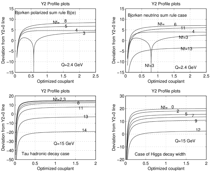
Figure 5: A plot showing similar one crossing point feature or solution $a_{4}$ of $Y_{2}$ for various QCD observables, spacelike and timelike, except for $N_{f}\leq 3$ in the spacelike cases, when $Y_{2}$ exhibits a double or triple crossing point feature.

3. When we compute next the crossing point features of $Y_{2}$ from eqn. (2), we find that in general for $N_{f}\leq 4$ the spacelike observables behave differently from the timelike observables. The $Y_{2}$ plots of these spacelike observables for $N_{f}\leq 3$, show a triple point crossing feature: $Y_{2}=b_{1},b_{2},b_{3},$ much like their $Y_{1}=a_{1},a_{2},a_{3}$ counterpart. The $N_{f}=3$ case of this $Y_{2}$ triple crossing feature can be seen in fig. 5. In contrast, for $N_{f}\geq 5$, all physical observables, spacelike and timelike, show only one $Y_{2}$ crossing point solution $a_{4}$ seen in fig. 5 and comparable to our earlier findings in paper [10]. The above triple $Y_{2}$ crossing behavior for $N_{f}\leq 3$ in the spacelike cases, will be found later to lead to a peculiar infrared cut off behavior of $Y_{2}$ relative to $Y_{1}$ in these low flavor states of spacelike observables.

4. We look closely next at the infrared cut off region of these spacelike and timelike observables. Taking first the cases of $N_{f}=5,6...$ for the spacelike observables and looking in their infrared cut off region shown in figs. 6 and 7, we see exactly the same two scale cut off structure, as that shown in figs. 2 and 3 for the timelike $R_{e+e-}(Q)$ case. The structures separate QCD dynamics in momentum transfer (or energy) space into three distinct regimes we have labelled in the figures as PQCD, CQCD, and hadron QCD.

5. Exactly this same two distinct scale cut off structure is exhibited for all flavor states $0\leq N_{f}\leq 8$ by the $\tau$ hadronic decay rate and the Higgs hadronic decay width observables shown in part in figs. 8 and  9. The figures compare well with figs. 2 and 3 of the $R_{e+e-}(Q)$ observable.

6. The peculiar cases of $N_{f}\leq 4,$ for spacelike observables are shown in figs. 10 to 12, to be compared with the same flavor state plots of timelike observables shown variously in figs. 2, 3, 8, and 9. We see that arising directly from the positive $\rho_{2}$ values in these $N_{f}\leq 4,$ flavor states of spacelike observables, their $Y_{2}$ and $Y_{1}$ curves tend to bunch together at the infrared cut off, with the $Y_{2}$ appearing to cut off earlier than the $Y_{1}$ curve for $N_{f}\leq 3$, though not for $N_{f}=4$. The bunching together tends to reduce the CQCD momentum gap or domain, compared to figs. 2 and 3, or figs. 6 to 9. However, the two scale infrared cut off structure still remains a finding, even in these positive $\rho_{2}$ spacelike cases.

7. Having seen that the two scale nonperturbative infrared structure persists in all flavor states $N_{f}\leq 8$, and for all observables spacelike and timelike, we now consider the paired numerical values of these scales, $Q_{c}(Y_{2})$ and $Q_{c}(Y_{1})$, and how these values vary from flavor to flavor and from one QCD observable (or perturbative series) to another. There are two obvious points at which we can evaluate and compare the two scales. We can evaluate the two scales at the point where each curve $Y_{2}$ and $Y_{1}$ independently begins to depart appreciably from its smoothly rising asymptotically free PQCD curve, to enter a nonperturbative QCD phase characterised by sudden rapidly rising coupling constant $a_{4}$ and $a_{3}$ respectively, in the infrared region. We shall denote the values of $Q_{c}(Y_{2})$ and $Q_{c}(Y_{1})$ so evaluated at this onset point of nonperturbative infrared QCD dynamics, by $Q_{on}(Y_{2})$ and $Q_{on}(Y_{1})$ respectively. The second obvious point where we can evaluate and compare the two scales is where each curve independently cuts off at the far infrared end, signalled by its coupling constant rising to infinite values $(a\geq 30$, or $\alpha_{s}\geq 100)$. We shall denote the two scales evaluted at this terminal infrared cut off point for each curve, by $Q_{c}(Y_{2})=Q_{off}(Y_{2})$ and $Q_{c}(Y_{1})=Q_{off}(Y_{1})$ respectively. A third obvious evaluation point exists in the special cases of $N_{f}\leq 4$ for spacelike observables, where as shown in figs. 10 to 12, the $Y_{2}$ curve exhibits a sudden turning away from the infrared region within the nonperturbative QCD regime, before finally rising up to infinity. This $Y_{2}$ infrared attractor point, provides a distinct coupling constant hierachy point at which we can also evaluate and compare the two infrared nonperturbative $Y_{2}$ and $Y_{1}$ scales.

8. Regarding the onset point of nonperturbative dynamics, we find from our various plots shown in figs. 2, 3, and 6 to 12, that the two curves $Y_{2}$ and $Y_{1}$ commence their transition into the nonperturbative regime at about the same critical coupling constant value, seen from the plots to lie in the range $0.18\leq a_{\mathrm{con}}\approx a_{\chi}\leq 0.28$, or $0.56\leq\alpha_{s}^{\mathrm{con}}\approx\alpha_{s}^{\chi}\leq 0.87$, where $a_{\mathrm{con}}$ denotes this critical coupling as evaluated on the $Y_{2}$ curve, while $a_{\chi}$ denotes the same nonperturbative onset critical coupling as evaluated on the $Y_{1}$ curves. If we look at the $Y_{2}$ plots as the more sharply focused indicator of this point of coupling constant criticality, we find from figs. 3, 8 and 9, that the $Y_{2}$ curves for different flavors tend actually to pass through a common point that lies around $a_{\mathrm{con}}\approx 0.25$, beyond which these various flavor lines cross paths and rise sharply to infinity. Basing on this, we can take as the mean onset critical coupling constant revealed by our plots for both $Y_{2}$ and $Y_{1}$, to be the value $a_{\mathrm{con}}\approx a_{\chi}=0.25$, Accordingly, we can evaluate and compare $Q_{on}(Y_{2})$ and $Q_{on}(Y_{1})$ at $a_{\mathrm{con}}\approx a_{\chi}=0.25$. The values of the two nonperturbative infrared scales evaluated at this point (I) and at the other two strategic points (III, and II) stated above, are shown in Tables 5 and 6.

9. Ignoring a few positive $\rho_{2}$ cases where specifically the $Y_{2}$ curve cut off widely earlier than the $Y_{1}$ curve as shown in plots (b) and (c) of fig 11, we find one running feature of the paired scales shown in Tables 5 and 6. This feature is that of the two nonperturbative infrared cut off scales $Q_{off}(Y_{2})$ and $Q_{off}(Y_{1})$, the lower one defined by the $Y_{2}$ solution occurs at a mean critical momentum cut off value of $Q_{off}(Y_{2})\approx 296$ MeV, well within a value we would associate with $\Lambda_{\mathrm{QCD}}$, the fundamental scale or constant of QCD. On the other hand, the upper cut off scale defined by $Q_{off}(Y_{1})$ occurs at a mean value: $Q_{off}(Y_{1})=1.44$ GeV. Both results are consistent with our earlier findings in paper [10] based on timelike $R_{e+e-}(Q)$ observable.

10. A second feature we observe readily from Tables 5 and 6, is that irrespective of the point of evaluation and the particular QCD observable considered, the two scales $Q_{c}(Y_{2})$ and $Q_{c}(Y_{1})$ are functions of flavor number $N_{f}$, both changing in value as the flavor number runs from $N_{f}=0$ to $N_{f}=8$. Here the spacelike and timelike QCD observables exhibit a distinct difference in their $N_{f}\leq 4$ states. Explicitly we find that for the timelike observables and for all $0\leq N_{f}\leq 8$, the two infrared scales move progressively apart as flavor increases. This can be seen directly in figs. 2, 3, 8 and 9. The same feature holds for spacelike observables but only for $N_{f}\geq 4$ shown in figs. 6 and 7. For $N_{f}<4$, Tables 5 and 6, and figs. 10 to 12 show that the spacelike observables exhibit a different pattern of flavor variation. With a view to later investigating what these patterns of flavor variation of the two nonperturbative infrared scales can mean, we have computed and shown in Tables 5 and 6, the ratio quantities $Q_{c}(Y_{2})/Q_{c}(Y_{1})$ of the two scales evaluated at one or the other of the three strategic couplant points mentioned above for various flavors and QCD observables. The ratios have been denoted I, II, II, depending on the point of evaluation of the $Y_{2},Y_{1}$ scales. Since this ratio gives a measure of the moving apart or the closing in of these two scales, we shall call the ratio a correlation factor between the two solutions $Y_{2}$ and $Y_{1}$ and the dynamical processes they cause or represent.

11. Summarizing, we can affirm that our curves not only define a three phase Padé QCD regime labelled PQCD, CQCD, and hQCD in our figures, but give us definite critical coupling constant values and critical momenta at which one transits from one Padé QCD regime into another. The extent these features and findings from Padé QCD lead us to conclude about physical QCD are what we examine next.

5 PHENOMENOLOGICAL FEATURES OF DYNAMICAL CHIRAL SYMMETRY BREAKING AND CONFINEMENT IN QCD

To see that the above Padé QCD infrared critical momenta $Q_{c}(Y_{1})$ and $Q_{c}(Y_{2})$ are amenable to interpretation as boundaries of the CQCD domain of physical QCD, we consider now some phenomenological features and attributes of dynamical chiral symmetry breaking $(D\chi SB)$ and quark confinement in QCD gleaned from a number of different sources and models, as follows:

1. Miransky [4] reviewing a broad spectrum of phenomenogical models of low energy QCD, in particular Bethe Salpeter wave function models of dynamical chiral symmetry breaking $(D\chi SB)$ and quark confinement, concluded that the momentum region of QCD where $D\chi SB$ takes place can be parameterized phenomenologically as: $\delta^{2}\leq Q^{2}\leq\Lambda_{\chi}^{2}$, where Q is the QCD operating momentum, while $\delta$ and $\Lambda_{\chi}$ are phenomenological infrared (IR) and ultraviolet (UV) cut-off momenta respectively, the values of which were phenomenologically found to be: $\delta\geq\Lambda_{\mathrm{QCD}}\approx 300$ MeV, and $\Lambda_{\chi}\approx 1$ GeV. The delta scale $\delta\approx\Lambda_{\mathrm{QCD}}$ was identified with the confinement scale of QCD, and was thus found phenomenologically to be at least a few times smaller than the $D\chi SB$ scale. These values are to be compared with our findings in Tables 5 and 6 where writing $Q_{off}(Y_{2})\leq Q_{\mathrm{CQCD}}\leq Q_{off}(Y_{1})$ as $\Lambda_{\mathrm{con}}\leq Q_{\mathrm{CQCD}}\leq\Lambda_{\chi}$, we found $\Lambda_{\mathrm{con}}=296$ MeV (mean value), while $\Lambda_{\chi}=1.44$ GeV (mean value), both for all $0\leq N_{f}\leq 8$ and for various physical observables, timelike and spacelike. The agreement is good.

2. Concerning the QCD critical coupling constant at the onset of $D\chi SB$, Refs. [4, 37, 38] found from their phenomenological estimates and approximations, the value: $\alpha_{s}^{\chi}\geq\pi/4$ meaning $a_{\chi}\geq 0.25$. The same value was arrived at by Higashijima [5] who found in his effective potential approaches, that chiral symmetry breaks down when his parameter $\lambda(t_{c})=3C_{2}(R)g^{2}/(4\pi^{2})>1$, where $C_{2}(R)=4/3$ for three color QCD, implying $\alpha_{s}^{\chi}=g_{c}^{2}/(4\pi)\geq\pi/4$, or $a_{\chi}\geq 0.25$. These phenomenological QCD critical couplings for $D\chi SB$ are to be compared with our exact finding in fig. 9 and other plots, that the various flavor lines converge and rise nonperturbatively at $a_{\mathrm{con}}\approx a_{\chi}\approx 0.25$, both for timelike and spacelike observables. The agreement is excellent.

3. Roberts and McKellar [39] solving numerically the Schwinger-Dyson (SD) integral equation for quark self energy (condensate), under varying kernel approximations, obtained the specific values: $\alpha_{s}^{\chi}=0.782$ in one kernel approximaion, and $\alpha_{s}^{\chi}=0.890$ in a more exact kernel evaluation. Their results then place $a_{\chi}$ in the range $0.253<a_{\chi}\leq 0.29$ for $N_{f}=0,4$ considered by them, to be compared again with our above Padé QCD finding in the general range: $0.18\leq a_{\chi}\leq 0.28$ for $0\leq N_{f}\leq 6$. The agreement is again excellent. Roberts and McKellar additionally found from their work that $D\chi SB$ and confinement do not necessarily occur together; rather the latter is held to occur subsequently, close to where the QCD coupling constant grows infinitely large as momentum transfer goes to zero. Our figs. 1 to 3, and figs. 6 to 12 manifest exactly this two scale feature and a sharply rising coupling constant to infinity, compatible with infrared slavery confinement at very low Q values.

4. Earlier work by Atkinson and Johnson [40] established the interesting point that there exists a critical value of QCD coupling constant, corresponding to the onset of chiral symmetry breaking, provided that (a) there is an infrared cutoff, realized phenomenologically as an effective gluon mass, and (b) there is an ultraviolet cutoff linked with a running coupling constant (a chiral symmetric phase of QCD). Within their own approximations to a fermion propagator Schwinger-Dyson equation, they find the critical QCD coupling constant for $D\chi SB$ to have the value $\alpha_{s}^{\chi}=0.91$. These findings from the Schwinger-Dyson ladder approximant equation agree again quite well with our Padé QCD two scale infrared NPQCD structure, and with the fact that our plots show $\alpha_{s}^{\chi}\approx 0.87$ at the upper limit.

5. In more recent studies, Guo and Huang [41] using two different approaches: (a) a semi-phenomenological self consistent equation to determine the quark condensate (the order parameter of $D\chi SB$) in the chiral limit, and (b) the usual Schwinger-Dyson equation (SD) improved by addition of gluon condensate kernel, obtained a critical QCD coupling $\alpha_{s}^{\chi}$ above which chiral symmetry breaks down. Their value is: $\alpha_{s}^{\chi}=0.2\pi$, which means $a_{\chi}=\alpha_{s}^{\chi}/\pi=0.2$. This again agrees very well with our Padé QCD findings seen in fig. 1 and figs. 7 to 10, and our specific mean value: $a_{\mathrm{con}}\approx a_{\chi}=0.25$.

6. Approaching our CQCD regime of QCD from the hadron end, in heavy ion Quark Gluon Plasma (QGP) studies, Lattice gauge theories and simulations [8, 42, 43], have evidence of the same two scale NPQCD structure found from our Padé QCD, and in the correct sequence. They find that the chiral symmetry restoration temperature $T_{\chi}$ is somewhat larger than the deconfinement temperature $T_{\mathrm{decon}}$. Put differently, Lattice QCD studies find that $D\chi SB$ is characterized by smaller distances compared to confinement distances. In our Padé QCD results played backwards, we expect our lower cut off momentum $Q_{off}(Y_{2})=\Lambda_{\mathrm{con}}$ to identify closely with $T_{\mathrm{decon}}$ as two parameters that mark confinement/deconfinement in QCD. Correspondingly, we expect our upper cut off momentum: $Q_{off}(Y_{1})=\Lambda_{\chi}$ to also identify closely with $T_{\chi}$ as two parameters that mark chiral symmetry breaking and restoration in QCD dynamics. Our Padé QCD finding that in general $\Lambda_{\chi}>\Lambda_{\mathrm{con}}$ then receives good support from the above independent Lattice QCD studies.

7. Explicitly, Shuryak [7] argued from a variety of phenomenological observations, including power corrections to deep inelastic scattering and heavy ion quark gluon plasma processes, that there must exist in the infrared region of QCD, a second scale other than the confinement scale, and that this second scale must be connected with chiral symmetry breaking. He estimated the hierachy of the two scales to be: $\Lambda_{\mathrm{\chi SB}}\gg\Lambda_{\mathrm{con}}\approx\Lambda_{\mathrm{QCD}}$, and that their ratio is of the order 3 - 5, meaning reciprocal ratios 0.33 - 0.20. Such two scale structure and hierachy in the infrared region of QCD is what we find here from our Padé perturbative QCD analysis shown variously in figs. 1 to 3 and figs. 6 to 12. Our $Q_{c}(Y_{2})/Q_{c}(Y_{1})$ ratios shown in Tables 5 and 6 for our two infrared scales are well within the estimates of Shuryak, depending on flavor.

8. In the context of effective Lagrangian theories of the strongly interacting regime of QCD where chiral symmetry breaking and quark confinement are believed to occur, Nambu and Jona-Lasinio (NJL) [3] were the first to introduce a viable effective Lagrangian model of hypothetical four fermion interactions, in which chiral symmetry breaking with pions as Goldstone bosons, was fully realized. The QCD scale at which the model worked entered the NJL effective Lagrangian theory as an upper cut-off momentum and was explicitly found to be $\Lambda_{\mathrm{\chi SB}}\approx 1$ GeV. Additionally, Nambu and Jona-Lasinio found that their effective theory works in a gap regime of QCD lying between the scale $\Lambda_{\mathrm{\chi SB}}\approx 1$ GeV and some lower hadronic scale $(\approx 300MeV)$ believed to be the onset point of quark confinement into hadrons. What we now observe is that this NJL model chiral symmetry breaking scale $\Lambda_{\mathrm{\chi SB}}\approx 1$ GeV, as well as the gap regime stretching to lower confinement scale, are exactly comparable with our finding from our Padé plots that, $296MeV\leq Q_{\mathrm{CQCD}}\leq 1.44GeV$, the implication of all this being that we identify our Padé CQCD domain with the NJL gap regime of Goldstone physics.

9. Another striking phenomenological model buttressing our Padé case is that of Manohar and Georgi [6] who not only found the phenomenological necessity for the two scale $(\Lambda_{\mathrm{\chi SB}},\Lambda_{\mathrm{con}})$ Goldstone physics structure and an intermediate infrared QCD regime bounded by $\Lambda_{\mathrm{con}}<Q<\Lambda_{\mathrm{\chi SB}}$ with $\Lambda_{\mathrm{\chi SB}}\gg\Lambda_{\mathrm{con}}\approx\Lambda_{\mathrm{QCD}}$, but actually proposed the use of the ratio of the two scales as a natural expansion parameter in chiral effective Lagrangian theories of low energy QCD. Their two scale structure has numerical values $\Lambda_{\mathrm{\chi SB}}\approx 1$ GeV, and $\Lambda_{\mathrm{con}}\approx 100-300$ MeV, both very close to our Padé QCD findings.

10. In their own novel gauge invariant nonperturbative approach to QCD at large distances, Gogohia and co-workers [44] found that a momentum free parameter $k_{o}$ in their approach, defined as some characteristic scale at which confinement and other nonperturbative ($D\chi SB)$ effects begin to play a dominant role in QCD, or more broadly defined as a momentum that separates the nonperturbative phase of QCD from the perturbative phase, always has both a lower and an upper boundary value which Gogohia et. al. found numerically to be: $635MeV\leq k_{o}\leq 775MeV$. Their more recent estimates [45, 46] give a higher value $\Lambda_{\mathrm{\chi}}\approx 1.2$ GeV, depending on input value for the pion decay constant. These result can be interpreted as a finding of a two scale structure in long distance QCD dynamics, and the explicit scale values estimated above by Gogohia et. al. are not incomparable with our paired scales shown in Tables 5 and 6 from Padé QCD.

11. From a completely different phenomenological perspective based on known masses of hadronic resonances, Greiner and Schafer [47] had also argued that the transition from NPQCD to PQCD must occur rapidly within a small segment of the energy scale they found to be $1\leq\sqrt{Q^{2}}\leq 3$ GeV such that NPQCD is definitely all of $Q\leq 1$ GeV, while all of $\sqrt{Q^{2}}\geq 3$ GeV is PQCD. Stated in our own terms, this Greiner-Schafer argument places the onset point of NPQCD/$D\chi SB$ in long distance QCD dynamics, in the range $1\leq\Lambda_{\chi}^{2}\leq 3$ GeV, or $1.0\leq\Lambda_{\chi}\leq 1.8$ GeV, to be compared with the values: $0.706\leq\Lambda_{\chi}\leq 2.6$ GeV for $N_{f}\leq 6$, we found from our Padé QCD and shown variously in Tables 5 and 6.

12. On the specific issue of the confinement scale in QCD, Brown and Pennington [48] obtained an infrared plot based on considerations of the Schwinger-Dyson equation for the gluon propagator, showing that the gluon propagator gets enormously enhanced and rises sharply in value to infinity in a Landau type cut-off behavior, at a scale $Q\approx\Lambda_{\mathrm{QCD}}$ in the infrared QCD region. This infrared gluon propagator behavior is normally taken as indicative of the point of onset of confinement in QCD. Its phenomenological scale found here at $Q=Q_{c}\approx\Lambda_{\mathrm{QCD}}$ is to be compared with our $a_{4}$ or $Y_{2}$ plots shown variously in figs. 2, 3, and figs. 6 to 9, which rise sharly to infinity at exactly similar critical momentum points $Q_{c}(Y_{2})\approx 296MeV\approx\Lambda_{\mathrm{QCD}}$.

13. The whole question of the enhanced $Q^{-4}$ infrared singularity behavior of the gluon propagator has actually become a central pivot for formulating chiral symmetry breaking and confinement dynamics of QCD, and estimating the the scale boundaries of these phenomena. Gogohia and Magradze [49] used it to establish a close interrelatedness and juxtaposed existence in QCD of dynamical chiral symmetry breaking and confinement, exactly as our Padé QCD finds in figs. 1 to 3 and 6 to 12. Arbuzov [50] working from the same premise of $Q^{-4}$ infrared singularity behavior of the gluon propagator, derives various essential attributes of spontaneous chiral symmetry breaking and other nonperturbative infrared QCD phenomena, and finds a momentum scale $k_{o}$ separating asymptotically free ultra violet QCD from the nonperturbative infrared domain to be $k_{o}=700$ MeV for the specific flavor state $N_{f}=0$ he considered. This Arbuzov value compares again very well with our value $\Lambda_{\chi}=706$ MeV for the same $N_{f}=0$, in the $R_{e+e-}(Q)$ values shown in Table 5. Other recent studies [46, 51, 52] of the nonperturbative QCD vacuum, assumed dominated by a $Q^{-4}$ gluon propagator behavior, are found to exhibit a two scale structure of chiral symmetry breaking and quark confinement dynamics, all strikingly similar to our Padé infrared QCD findings reported here.

14. Finally Iwasaki and co-workers [53] found from their Lattice QCD studies that dynamical chiral symmetry breaking and confinement in infrared QCD must be closely related or correlated, even when they found no evidence that the two phenomena necessarily occur simultaneously. The implication for scale considerations, is that the two phenomena are compatible with being intrinsic two scale structure or sequential phenomena of infrared QCD dynamics, exactly as we find here with infrared Padé QCD. What is more, Iwasaki et. al. found that their two scales and phenomena of infrared QCD, depend on the flavor number $N_{f}$ of the QCD system, again exactly as our Tables 5 and 6, and our various Padé QCD plots, explicitly show.

Clearly, these varied physical QCD phenomenological results concerning infrared QCD dynamics and its critical boundary points, all consistently close to and in agreement with the Padé QCD findings shown variously in figs. 1 to 3, and figs. 6 to 10, as well as Tables 5 and 6, compel us to admit the Padé infrared $(a_{3},a_{4})$ structures as relating to physical QCD. In that case, we can make a number of important deductions from our work, concerning infrared dynamics of physical QCD as follows.

6 FAVORED FLAVOR STATES FOR QUARK CONFINEMENT IN QCD

One immediate deduction or proposal we can make following from the above, is that confinement and chiral symmetry breaking in QCD are caused by two distinct component color forces or dynamics of QCD. Of our two nonperturbative infrared couplant forces $Y_{2}$ and $Y_{1}$, the latter is responsible for and identifiable with the onset and dynamics of chiral symmetry breaking in QCD, while the former $Y_{2}$ is responsible for quark confinement in QCD. Following from the fact that the two component color forces are independent solutions $a_{3}$ and $a_{4}$ of our Padé couplant equation, we assert as part of our finding, that the two nonperturbative infrared QCD phenomena, chiral symmetry breaking and quark confinement, are actually distinct physical phenomena. They may however still be closely related in the sense that one phenomenon provides a stimulus or background that facilitates the occurrence of the other phenomenon.

The indication from our plots is that dynamical chiral symmetry breaking $(D\chi SB)$ occurs first at the higher infrared nonperturbative scale $Q_{c}(Y_{1})$, phenomenologically flooding the QCD vacuum with $q\bar{q}$ pair condensates, which in turn provide a superconducting state of QCD vacuum, compatible with quark confinement in the manner advocated by a number of workers [54, 55, 56]. However, what our work now indicates is that confinement itself does not actually occur (even after a $D\chi SB$) until the independent $Y_{2}$ confinement causing color force has attained its own confinement scale at $Q=Q_{c}(Y_{2})<Q_{c}(Y_{1})$. In such a scenario, the possibility arises that if these two scales are very far apart, the condensate background effect caused by $Y_{1}$ at scale $Q_{c}(Y_{1})$ may become dissipated or ineffective by the time we reach the $Y_{2}$ confining scale at $Q_{c}(Y_{2})$. Then confinement does not occur even though we are at scale $Q_{c}(Y_{2})$.

The details of this confinement mechanism do not concern us here. What we show now is that our work provides a strong evidence or indication that the above interrelatedness or correlation of confinement with dynamical chiral symmetry breaking does exist in concrete terms in QCD. Here we return to Table 5 and 6 where we already computed the ratios $Q_{c}(Y_{2})/Q_{c}(Y_{1})$ as a measure of how close together or far apart the two nonperturbative infrared scales are. We now plot this $Q_{c}(Y_{2})/Q_{c}(Y_{1})$ correlation factor as a function of flavor number and for different spacelike and timelike observables. The plots are shown in fig. 13, and reveal some interesting features.

We observe that in the spacelike cases the correlation ratio first rises with increasing flavor number from $N_{f}=0$, and reaches a peak at $N_{f}=2$ or in the region $1\leq N_{f}\leq 3$. It then falls off rapidly for all $N_{f}\geq 4$ and is practically zero near $N_{f}=7,8$. It is well known in nature, that the most stable hadrons and confined quark states are the $(u,d)$ or $N_{f}=2$ states of QCD. These are the nucleons (protons and neutrons). $N_{f}=3$ confined quark states exist as higher baryon states that are only quasi stable. There are no known stable or quasi stable confined quark states of flavor number $N_{f}\geq 4$. Our fig. 13 appears therefore to be providing us a strikingly direct explanation and insight into the origin of this well known state of affairs in nature, attributing it to an interplay or some intrinsic interrelatedness of dynamical chiral symmetry breaking and quark confinement mechanism in QCD.

In the case of the timelike $Q$ cases shown also in fig. 13, the correlation factor falls off progressively from $N_{f}=0$ to $N_{f}=8$, in a manner to suggest that the most readily confined QCD states are the pure gluonic states or glue balls, rather than the $1\leq N_{f}\leq 3$ states. This would appear not to be so in nature but we are not able at the moment to reconcile this crucial difference in the timelike and spacelike behaviors of fig. 13, except that the difference is directly traceable to $\rho_{2}$ being positive or negative in the manner shown in Table 1. Apart from this difference in their $N_{f}\leq 3$ behavior, the timelike and spacelike observables are fully in agreement from their correlation plots shown in fig. 13, that confinement becomes rapidly less probable for $N_{f}\geq 4$, and that this decline arises from the intrinsic confinement scale $Q_{c}(Y_{2})$ becoming progressively less correlated with the intrinsic dynamical chiral symmetry breaking scale $Q_{c}(Y_{1})$ of QCD.

We remark that Iwasaki and co-workers [53] actually found in their Lattice QCD studies, that confinement and dynamical chiral symmetry breaking cease to occur for $N_{f}\geq 7$, but occur only for $N_{f}\leq 6$. Our work and fig. 13 explain adequately what Iwasaki and co-workers observed in their Lattice QCD studies, and this close agreement between their work and ours, leads us once more to affirm that our Padé infrared QCD results have a physical reality, reproducing quite well infrared QCD dynamics from a wide variety of phenomenological considerations, including Lattice QCD simulations.

7 FROZEN COUPLANT VERSUS INFRARED SLAVERY STRUCTURE OF CQCD

A second deduction for QCD we can make from our Padé plots and features, is that while many of the phenomenological models we cited earlier in this paper, especially those dealing with ladder approximant Schwinger-Dyson equations, make mere guesses or assumptions about the form of the QCD coupling constant inside the CQCD regime, $(\Lambda_{\mathrm{con}}\leq Q\leq\Lambda_{\chi})$, some authors parameterizing it by a frozen coupling constant or a step function:

$$g^{2}((q-p)^{2})=\theta(q^{2}-p^{2})g^{2}(q^{2})+\theta(p^{2}-q^{2})g^{2}(p^{2})$$ (35)

with

$$\theta(q^{2}-p^{2}) = 1,\mbox{if $q^{2}>p^{2}$}$$ (36)

$$= 0,\mbox{if $q^{2}<p^{2}$}$$

or in the form:

$$g^{2}(q^{2}) = \frac{2}{b\ln\left(\frac{(q_{c}^{2}+q^{2})}{\Lambda_{\mathrm{QCD}}^{2}}\right)}$$ (37)

$$= \frac{2}{b\ln\left(\frac{q^{2}}{\Lambda_{\mathrm{QCD}}^{2}}\right)},for:q>q_{c}$$

$$= \frac{2}{b\ln\left(\frac{q_{c}^{2}}{\Lambda_{\mathrm{QCD}}^{2}}\right)},for:q\leq q_{c}$$

where $q_{c}$ is some constant parameter identifiable with our $\Lambda_{\chi}$, our Padé model shows explicitly [10] that the $N_{f}\leq 8$ flavor states are not infrared couplant freezing states of QCD. Rather the two coupling constant solutions $a_{3}$ and $a_{4}$ that govern QCD dynamics in this CQCD infrared regime of QCD are together growing infinitely large in the domain. Such infinitely growing coupling constant in the infrared region of QCD, is what is naturally needed to explain physical confinement of colored quarks and gluons into hadrons. Therefore, our optimized Padé QCD has this additional positive side to it that it offers a more natural explanation of the origin and mechanism of quark confinement than some of the phenomenological models we cited in section 5. Indeed the $Q^{-4}$ enhanced infrared singularity structure of the gluon propagator, currently gaining ground [46, 50, 51, 52] as a necessary ingredient to reconcile QCD vacuum with quark confinement, the linearly rising inter-quark potential law, and other nonperturbative features of infrared QCD, has no place for an infrared fixed point in low flavor states of QCD. The same conclusion that low flavored states of QCD do not manifest any infrared stable fixed point is found in several other places Refs. [57] to [66], all rather contrary to Refs. [67, 68].

8 SUMMARY AND CONCLUSIONS

Summarizing, we state that the two scale cut off momentum structure exhibited in the infrared region of QCD by our optimized Padé couplant eqns. (1) and (2), is identifiable as marking the points of onset of dynamical chiral symmetry breaking and quark confinement respectively, in infrared QCD. Taking these two infrared nonperturbative phenomena of QCD as characteristically marking the beginning phase and end phase respectively, of the CQCD regime of QCD, we can conclude, based on extensive correlations of our results with a wide range of known phenomenological studies of low energy QCD, that our work actually constitutes a finding from within perturbative QCD approaches, of a previously unknown but long speculated infrared QCD window, marked at its two ends by a critical coupling constant and a critical momentum, and separating QCD dynamics in the cold (zero temperature vacuum state), into the three distinct phases of purely hadronic QCD at very low momentum transfers Q, a largely weak perturbative QCD phase at high Q, and finally an intermediate phase or regime of strongly coupled yet quark-gluon dominated QCD dynamics.

Traditionally in perturbative QCD (PQCD), one believes that an impenetrable wall at $Q=\Lambda_{\mathrm{QCD}}$ shuts out nonperturbative QCD and hadron physics from any view or access from the PQCD end. This apart, it is held that much of PQCD remains accessible in the domain stretch from the far ultraviolet (UV) QCD, until close to the Landau cut off wall at $Q=\Lambda_{\mathrm{QCD}}$. What our work shows is that while the Landau wall at $Q=Q_{c}(Y_{2})\approx 296MeV\approx\Lambda_{\mathrm{QCD}}$ remains impenetrable from the PQCD end, much of the most important aspects of nonperturbative QCD dynamics including spontaneous chiral symmetry breaking and the confinement of quarks into hadrons, actually lies in a buffer zone (CQCD) that leads up from the far UV QCD to the Landau wall. Beyond the Landau wall lies pure hadron physics, and our work provides explicit boundary values both in critical momentum and critical QCD coupling constant, separating these three phases of QCD, as delineated from the PQCD beta function parameters and renormalization group equations of a running QCD coupling constant.

We believe the same CQCD buffer zone just delineated, is what is currently being observed as Quark Gluon Plasma (QGP) from the hadron end at high temperature (non-vacuum QCD state), in heavy ion experiments at CERN and Brookhaven (RHIC). As such, it becomes immediately possible to ask how the domain boundaries and dynamical characteristics of this intermediate CQCD/QGP phase of QCD get modified or shifted at two widely separated temperatures and energy density, represented by the heavy ion experiments on the one hand, and our zero temperature vacuum QCD studies on the other hand. This comparison will await further developments and evolution in the QGP plasma experiments and the various Lattice and phenomenological computations relating thereto.

Focusing on our own boundary values of the CQCD regime computed here at zero temperature, we found that these values in general vary with flavor as seen from Tables 5 and 6, and from our various figures and plots. We have interpreted this $Q_{c}(Y_{2})/Q_{c}(Y_{1)}$ flavor behavior to be a maifestation of a phenomenologically known fact that dynamical chiral symmetry breaking and quark confinement are closely related infrared QCD phenomena. Our specific finding is that the more widely separated their set scales are, the less likely the corresponding flavor state of QCD will be a quark confinement state. We actually found evidence from our fig. 13 that quark confinement occurs mainly in the low flavor states $N_{f}\leq 3$, with a peak at $N_{f}=2$, but becomes progressively non-existent or improbable in the higher flavor states $N_{f}=4,5,6,7,8$. It turns out that this is actually what one finds in nature.

After we had completed this work, our attention was drawn to a preprint by Elias and co-workers [69] in which they used their own method of denominator versus numerator zeros of Padé QCD beta function, to estimate the location and scale value of the point where perturbative QCD cuts off from the infrared region. They found only one scale cut-off point at a critical momentum $\mu_{c}\approx 1.0$ GeV. This is in contrast to our two scale cut off structure presented variously in this paper, and anticipated in the several phenomenological models we cited in section 5 of this paper. We make two comments in relation to this work of Elias et. al. The first is that the method of denominator versus numerator zero of Padé beta function appears not adequate to reveal the multicomponent couplant solutions of Padé QCD and consequently the two scale infrared structure. This fact was already highlighted in our earlier paper [10]. One needs to work with effective charges and renormalization group invariants or optimized Padé QCD. The second comment we make is one of noting that the one scale cut off found by Elias et. al. at $\mu_{c}\approx 1.0$ GeV, is comparable to our chiral symmetry breaking scale $\Lambda_{\chi}\approx 1.44$ GeV. Since Elias et. al. worked with the higher Padé approximants $[2|1],[1|2],[3|1],[1|3],[2|2]$, as against our $[1|1]$ Padé approximant, the close agreement between our onset scale and theirs, provides a good indication that our results and features presented here will hold irrespective of the particular Padé approximant used, exactly as we already inferred in paper [10]. One could of course repeat directly the various computations reported in this paper, using this time, these higher Padé approximants to verify that the results remain robust. The draw back is that the higher renormalization scheme invariants $\rho_{3},\rho_{4}...$ needed for such computations, are not presently known or computed perturbatively for the various QCD physical observables reported in this paper.

ACKNOWLEDGEMENTS
The author thanks Dr. Billy Bonner, Director T.W. Bonner Nuclear Laboratory, Rice University, Houston, for hospitality. He is particularly grateful to Dr. Awele Ndili of Stanford University, California, for much technical advice on computing and software. He thanks the following colleagues who kindly read an earlier version of this paper and made suggestions for improvement: Dr. V. Miransky and Dr. V. Elias of Western Ontario Canada, Dr. B. McKellar of Melbourne Australia, Dr. K. Higashijima of Osaka Japan, and Dr. V. Gogokhia of Budapest Hungary. Finally, the author thanks Fredna Associates for financial support that made this work possible.

Table 1: Computed $\rho_{2}(N_{f})$ values for various spacelike and timelike QCD observables

Flavor	$\rho_{2}^{Bj(e)}$	$\rho_{2}^{Bj(\nu)}$	$\rho_{2}^{GLS(\nu)}$	$\rho_{2}^{(e^{+}e^{-})}$	$\rho_{2}^{(\tau)}$	$\rho_{2}^{(H)}$
Number
$N_{f}$
0	17.9244	15.9567	17.9244	-8.410032589173554	1.8089	-17.8458
1	13.7474	12.3442	13.3343	-9.996607149709793	-0.5654	-18.9820
2	9.6051	8.7025	8.7787	-10.91120013471925	-2.9879	-20.1684
3	5.4757	5.0067	4.2361	-12.20710268197531	-5.4756	-21.4108
4	1.3304	1.2238	-0.3223	-13.90995802777778	-8.0508	-22.7170
5	-2.8695	-2.6906	-4.9354	-15.49181836878120	-10.7438	-24.0975
6	-7.1775	-6.7981	-9.6566	-17.66469557734694	-13.5963	-25.5668
7	-11.6698	-11.1857	-14.5620	-19.78668878025239	-16.6675	- 27.1456
8	-16.4581	-15.9819	-19.7635	-22.74511792421761	-20.0446	-28.8640
9	-21.7139	-21.3833	-25.4325	-25.96983971428571	-23.8613	-30.7687
10	-27.7143	-27.7079	-31.8461	-30.64825148592373	-28.3334	-32.9345
11	-34.9379	-35.5045	-39.4829	-36.70527878387512	-33.8340	-35.4912
12	-44.2885	-45.8101	-49.2467	-46.58505774333333	-41.0672	- 38.6836
13	-57.7031	-60.8467	-63.0745	-63.56012999671129	-51.5427	-43.0365
14	-80.2178	-86.3914	-86.0023	-101.9145678055556	-69.1847	-49.9139
15	-130.2979	-143.6271	-136.4956	-229.8874551066667	-108.3829	-64.3179
16	-374.1328	-423.2004	-380.7437	-1724.404563921111	-298.6440	-131.2671

Table 2: $Y_{1}$ structural parameters $Q_{\mathrm{min}},a_{1}(Q_{\mathrm{min}}),Q_{\mathrm{max}}$ and $a_{3}(Q_{\mathrm{max}})$ for Bjorken sum rule $\rho_{2}^{Bj(e)}$ values shown in Table 1 in optimized $[1|1]$ Padé QCD. The $N_{f}=0,1,2$ cases were computed using $\sqrt{|D|}.$

Flavor Number $N_{f}$	$Q_{\mathrm{min}}$ (GeV)	$a_{1}(Q_{\mathrm{min}})$	$Q_{\mathrm{max}}$ (GeV)	$a_{3}(Q_{\mathrm{max}})$
0	16.3391	0.0812	633.07	0.10006
1	12.5361	0.0936	444.10	0.1174
2	8.0622	0.1164	325.33	0.15139
3	6.11284	0.13944	364.81	0.18538
4	11.1934	0.12027	238.4	0.1477
5	17.012	0.1149	204.84	0.1344
6	24.2354	0.11425	161.30	0.1278
7	32.592	0.11665	115.8	0.1243
8	36.214	0.12191	37.56	0.12235
9	6.910	0.12087	36.279	0.1303
10	0.3015	0.11868	62.46	0.1428
11	1.036$(10^{-3})$	0.1143	250.952	0.16116
12	8.2160$(10^{-7})$	0.1059	7.7850$(10^{+3})$	0.1900
13	9.029$(10^{-14})$	0.0918	7.8324$(10^{+7})$	0.2395
14	9.752$(10^{-35})$	0.07130	7.8451$(10^{+20})$	0.3652
15	1.281$(10^{-101})$	0.0448	$\approx 1.0(10^{+85})$	$>0.80$
16	2.250$(10^{-176})$	0.01520	$\gg 10^{+308}$	$\gg 1.0$

Table 3: Bjorken neutrino sum rule $Y_{1}$ structural parameters $Q_{\mathrm{min}},a_{1}(Q_{\mathrm{min}}),Q_{\mathrm{max}}$ and $a_{3}(Q_{\mathrm{max}})$ computed using the $\rho_{2}^{Bj(\nu)}$ values shown in Table 1, in optimized $[1|1]$ Padé QCD. The $N_{f}=0,1,2$ cases were computed using $\sqrt{|D|}$.

Flavor Number $N_{f}$	$Q_{\mathrm{min}}$ (GeV)	$a_{1}(Q_{\mathrm{min}})$	$Q_{\mathrm{max}}$ (GeV)	$a_{3}(Q_{\mathrm{max}})$
0	16.271	0.0868	404.4	0.1087
1	12.432	0.1005	403.6	0.1284
2	7.63	0.1285	326.6	0.1724
3	8.5585	0.1312	266.8	0.171
4	13.5895	0.1194	732.4	0.1464
5	19.388	0.1159	281.4	0.1357
6	26.4586	0.1159	343.3	0.1299
7	34.4886	0.1186	113.8	0.1265
8	37.52	0.1237	39.72	0.12415
9	5.117	0.1219	37.18	0.1315
10	0.2723	0.1187	64.03	0.1430
11	1.678$(10^{-3})$	0.1133	260.28	0.1590
12	8.130$(10^{-8})$	0.10402	8.2617$(10^{+3})$	0.1835
13	9.620$(10^{-15})$	0.0897	8.592$(10^{+7})$	0.2255
14	6.69$(10^{-42})$	0.06957	8.9984$(10^{+20})$	0.3253
15	3.440$(10^{-83})$	0.0441	1.02687$(10^{+85})$	1.465
16	4.90$(10^{-307})$	0.015040	$\gg 10^{+305}$	$\gg 10.0$

Table 4: Tau($\tau$) Hadronic decay $Y_{1}$ structural parameters $Q_{\mathrm{min}},a_{1}(Q_{\mathrm{min}}),Q_{\mathrm{max}}$ and $a_{3}(Q_{\mathrm{max}})$ computed using the $\rho_{2}^{\tau}$ values shown in Table 1, in optimized $[1|1]$ Padé QCD. All $D$ values in this case, including $N_{f}=0$ state, are positive.

Flavor Number $N_{f}$	$Q_{\mathrm{min}}$ (GeV)	$a_{1}(Q_{\mathrm{min}})$	$Q_{\mathrm{max}}$ (GeV)	$a_{3}(Q_{\mathrm{max}})$
0	26.6430	0.0773	765.30	0.0942
1	32.0952	0.07825	1697.95	0.0942
2	38.7402	0.07977	749.06	0.09475
3	46.851	0.08194	785.50	0.0959
4	56.716	0.0849	813.4	0.09772
5	68.5620	0.08893	660.9	0.10015
6	82.1620	0.09422	547.18	0.1033
7	95.261	0.10123	267.0	0.10692
8	92.2863	0.11058	95.54	0.11094
9	15.2460	0.1147	81.01	0.1232
10	0.591	0.1172	122.64	0.1407
11	3.5330$(10^{-3})$	0.1164	435.71	0.1654
12	1.2110$(10^{-6})$	0.11016	1.2066$(10^{+4})$	0.2035
13	2.015$(10^{-14})$	0.0964	1.09640$(10^{+8})$	0.2728
14	3.505$(10^{-33})$	0.0745	1.00163$(10^{+21})$	0.4690
15	2.636$(10^{-105})$	0.0463	$\geq 1.0(10^{+88})$	$\gg 1.0$
16	$1.0610^{-295}$	0.0153	$\gg 10^{+305}$	$\gg 1.0$

Table 5: CQCD boundary momenta $Q_{c}(Y_{1})$ and $Q_{c}(Y_{2})$ computed for various physical observables or effective charges in the $[1|1]$ optimized Padé QCD. The $Q_{c}(Y_{1}),Q_{c}(Y_{2})$ values are taken from figs. 2, 3, and figs. 6 to 12, at the three strategic couplant points discussed in the paper. Ratio I = $Q_{on}(Y_{2})/Q_{0n}(Y_{1})$, while Ratio III = $Q_{off}(Y_{2})/Q_{off}(Y_{1})$. Ratio II was evaluated at the IR attractor point of the $Y_{2}$ curve where this exists.

QCD	Flavor	$Q_{on}(Y_{2})$	$Q_{on}(Y_{1})$	Ratio	$Q_{off}(Y_{2})$	$Q_{off}(Y_{1})$	Ratio
observable	$N_{f}$	GeV	GeV	I	GeV	GeV	III/II
Bj(e)	0	1.0	2.375	0.4211	0.8791	0.9465	0.9287
	1	1.195	2.50	0.4780	1.0956	0.900	1.2173
	2	1.60	2.825	0.5664	1.5661	0.8380	1.8689
‘	3	1.815	3.25	0.5585	0.85	0.81	1.0494
	4	1.09	3.186	0.3421	0.78278	0.88625	0.8833
	5	0.8125	3.60	0.2257	0.3953	0.98629	0.4008
	6	0.6340	4.25	0.1492	0.2450	1.1392	0.2150
	8	0.440	7.80	0.0564	0.1084	1.900	0.0571
Bj($\nu$)	0	1.4474	2.9460	0.4913	1.349312	1.9650	0.6867
	1	1.7177	3.10	0.5541	1.66233	2.3360	0.7116
	2	2.4460	3.8150	0.6412	-	-	-
	3	1.9365	3.760	0.5150	1.856	2.5780	0.7199
	4	1.30	3.910	0.3325	0.911941	1.3602	0.6704
	5	0.95	4.10	0.2317	0.4732	1.15174	0.4109
	6	0.75	4.870	0.1540	0.290	1.2941	0.2241
	8	0.4710	8.0	0.0589	0.1225	2.0593	0.0595
$R_{e+e-}(Q)$	0	0.3700	1.700	0.2176	0.2364	0.7064	0.3347
	1	0.350	1.850	0.1892	0.20996	0.7345	0.2859
	2	0.337	2.05	0.1644	0.19005	0.7611	0.2497
	3	0.320	2.175	0.1471	0.16717	0.80043	0.2089
	4	0.3037	2.625	0.1157	0.1425	0.8599	0.1657
	5	0.2875	3.00	0.0958	0.1204	0.9420	0.1278
	6	0.270	3.800	0.0711	0.09771	1.07991	0.0905
	7	0.250	4.80	0.0521	0.079425	1.320	0.0602
	8	0.249	7.25	0.0343	0.06250	1.8115	0.0345
$\tau$ decay	0	1.2446	3.373	0.369	1.07444	1.340	0.8018
$R^{(\tau)}$	1	1.1341	3.674	0.3087	0.8308	1.3980	0.5943
	2	1.025	4.0	0.2562	0.6615	1.468	0.4506
	3	0.9340	4.50	0.2076	0.5305	1.560	0.3401
	4	0.850	5.237	0.1623	0.42325	1.6825	0.2516
	5	0.7756	6.250	0.1241	0.3331	1.8540	0.1796
	6	0.700	7.50	0.0933	0.260	2.146	0.1212
	8	0.6170	14.70	0.0420	0.15226	3.590	0.0424

Table 6: Further data on CQCD boundary momenta $Q_{c}(Y_{1})$ and $Q_{c}(Y_{2})$ computed for various physical observables or effective charges in the $[1|1]$ optimized Padé QCD. The $Q_{c}(Y_{1}),Q_{c}(Y_{2})$ values are taken from figs. 2, 3, and figs. 6 to 12, at the three strategic couplant points discussed in the paper. Ratio I = $Q_{on}(Y_{2})/Q_{0n}(Y_{1})$, while Ratio III = $Q_{off}(Y_{2})/Q_{off}(Y_{1})$. Ratio II was evaluated at the IR attractor point of the $Y_{2}$ curve where this exists.

QCD	Flavor	$Q_{on}(Y_{2})$	$Q_{on}(Y_{1})$	Ratio	$Q_{off}(Y_{2})$	$Q_{off}(Y_{1})$	Ratio
observable	$N_{f}$	GeV	GeV	I	GeV	GeV	III/II
Bj(e)	0				0.879030	1.36	0.6463
	1				1.0956	1.58	0.6934
	2				1.5661	2.24	0.6992
‘	3				1.7941495	2.600	0.6906
	4				0.782782	1.190	0.6578
	5				0.3953	0.98629	0.4008
	6				0.2450	1.1392	0.2150
	8				0.1084	1.900	0.0571
$\tau$ decay	0				1.021127	1.6610	0.6148
$R^{(\tau)}$	1				0.829744217	1.45260	0.5712
	2				0.6615	1.468	0.4506
	3				0.5305	1.560	0.3401
	4				0.42325	1.6825	0.2516
	5				0.3331	1.8540	0.1796
	6				0.260	2.146	0.1212
	8				0.15226	3.590	0.0424
Higgs case	0	0.6212	4.13	0.1504	0.37228	1.7615	0.2113
$R^{(H)}$	2	0.600	5.50	0.1091	0.3180	2.0644	0.1540
	3	0.600	6.50	0.0923	0.28940	2.2825	0.1268
	4	0.550	7.10	0.0775	0.26075	2.5868	0.1008
	5	0.550	9.00	0.0611	0.23280	3.0260	0.0769
	6	0.570	12.50	0.0456	0.2065	3.720	0.0555

Figure 4: A plot showing similar $Y_{1}$ triple point crossing feature or solutions $a_{1},a_{2},a_{3}$ for various physical observables, spacelike and timelike, exactly as for the $R_{e+e-}(Q)$ observable discussed in paper [10].

Figure 6: A two scale cut off structure of $a_{3}$ and $a_{4}$ in the infrared region: The case of Bjorken polarized sum rule Bj(e), (spacelike).

Figure 7: A two scale cut off structure of $a_{3}$ and $a_{4}$ in the infrared region: The case of Bjorken neutrino sum rule Bj($\nu$), (spacelike).

Figure 8: A two scale cut off structure of $a_{3}$ and $a_{4}$ in the infrared region: The case of tau hadronic decay rate, (timelike).

Figure 9: A two scale cut off structure of $a_{3}$ and $a_{4}$ in the infrared region: The case of Higgs hadronic decay width, (timelike).

Figure 10: The $N_{f}=2$ infrared cut offs of $Y_{1}$ and $Y_{2}$ plotted for two spacelike observables for which $\rho_{2}$ is positive and large, and $D$ is negative. The cut off curves are seen to bunch closely together.

Figure 11: The cases of $N_{f}=0,1$, infrared cut off structure of $Y_{1}$ and $Y_{2}$ for the two spacelike observables, Bj(e) and Bj($\nu$) for which $\rho_{2}$ is positive and large, and $D$ is negative

.

Figure 12: A plot showing the $Y_{2}$ cut off behavior in the $N_{f}=3,4$ flavor states of positive $\rho_{2}$ but positive $D$, in spacelike physical observables, Bj(e), Bj($\nu$), and Gross - Llewellyn Smith (GLS) sum rules. The cut offs $a_{3},a_{4}$ are seen to occur closely together, with $a_{4}$ even growing faster than $a_{3}$ in the ensuing CQCD dynamics in $N_{f}=3$ case

.

Figure 13: A plot showing the strong correlation between dynamical chiral symmetry breaking and quark confinement in QCD as revealed in Padé infrared couplant structures. Quark confinement is seen to be most favored in $N_{f}\leq 3$ states with a peak at $N_{f}=2$, but drops rapidly to zero for $N_{f}\geq 4$, exactly as one finds in nature. Each curve was normalized to its $N_{f}=0$ flavor state.

References

- [1] H. Leutwyler, Ann. Phys. (N.Y.), 235, 165 (1994); also J. Gasser and H. Leutwyler, Ann. Phys. (N.Y.) 158, 142 (1984), and Nucl. Phys. B250, 465 (1985)
- [2] S. Weinberg, Physica, A96, 327 (1979).
- [3] Y. Nambu and G. Jona-Lasinio, Phys. Rev. 122, 345 (1961)
- [4] V. A. Miransky, Dynamical Symmetry Breaking in Quantum Field Theories, Chapter 12, (World Scientific Publishers, Singapore, 1993).
- [5] K. Higashijima, Suppl. Prog. Theor. Phys. 104, 1 (1991) ; also K. Higashijima, in Proceedings of the KEK Summer Institute on High Energy Phenomenology, KEK 91-8, August (1990), and Phys. Rev. D29, 1228 (1984).
- [6] A. Manohar and H. Georgi, Nucl. Phys. B234, 189 (1984).
- [7] E. Shuryak, Phys. Lett. 107B, 103 (1981)
- [8] P. van Baal (Editor), Confinement, Duality, and Nonperturbative Aspects of QCD, Proceedings NATO Advanced Science Institutes Series, Physics, Vol. 368, Plenum Press, New York, (1998)
- [9] T. Bhattacharya, R. Gupta and A. Patel (Editors), Lattice 2000, Proceedings of the XVIIIth Intern Symposium on Lattice Field theory, Bangalore, India, Nucl. Phys. B (Proc. Suppl), Vol.94, North Holland Publishers, 2001.
- [10] F. N. Ndili, Phys. Rev. D64, 014018 (2001).
-
[11]
D. J. Gross and F. Wilczek, Phys. Rev. Lett. 30, 1343 (1973);
H. D. Politzer, Phys. Rev. Lett. 30, 1346 (1973). -
[12]
W. E. Caswell, Phys. Rev. Lett. 33, 244 (1974);
D. R. T. Jones, Nucl. Phys. B75, 531 (1974);
E. S. Egorian and O. V. Tarasov, Teor. Mat. Fiz. 41, 26 (1979) -
[13]
O. V. Tarasov, A. A. Vladimirov and A. Yu. Zharkov, Phys. Lett. B93, 429 (1980);
S. A. Larin and J. A. M. Vermaseren, Phys. Let. B303, 334 (1993). - [14] T. van Ritbergen, J. A. M. Vermaseren and S. A. Larin, Phys. Lett. B400, 379 (1997); J. A. M. Vermaseren, S. A. Larin and T. van Ritbergen, Phys. Lett. B405, 327 (1997).
- [15] P. M. Stevenson, Phys. Rev. D23, 2916 (1981).
- [16] P. M. Stevenson, Phys. Rev. D33, 3130 (1986)
- [17] A. Dhar, Phys. Lett. 128B, 407 (1983).
- [18] A. Dhar and V. Gupta, Phys. Rev. D29, 2822 (1984).
- [19] G. Grunberg, Phys. Rev. D29, 2315 (1984); and Phys. Lett. 95B, 70 (1980).
- [20] D. I. Kazakov and D. V. Shirkov, Sov. J. Nucl. Phys. 42, 487 (1985).
- [21] J. Chyla, Phys. Rev. D40, 676 (1989).
- [22] J. D. Bjorken, Phys. Rev. 148, 1467 (1966); Phys. Rev. D1, 1376 (1970).
- [23] S. A. Larin and J. A. M. Vermaseren, Phys. Letts. B 259, 345 (1991).
- [24] S. A. Larin, F. V. Tkachov and J. A. M. Vermaseren, Phys. Rev. Letts. 66, 862 (1991).
- [25] D. J. Gross and C. H. Llewellyn Smith, Nucl. Phys. B 14, 337 (1969).
- [26] J. Chyla, and A. L. Kataev Phys. Letts. B 297, 385 (1992).
- [27] S. G. Gorishny, A.L. Kataev and S. A. Larin, Phys. Letts. B 259, 144 (1991).
- [28] L. R. Surguladze and M. A. Samuel, Phys. Rev. Letts. 66, 560 (1991).
- [29] G. Chetyrkin, A.L. Kataev and F. V. Tkachov, Phys. Letts. B85, 279 (1979).
- [30] M. Dine and J. Sapirstein. Phys. Rev. Lett. 43, 668 (1979).
- [31] W. Celmaster and R. Gonsalves, Phys. Rev. Lett. 44, 560 (1980).
- [32] J. Chyla, A. Kataev and S. A. Larin, Phys. Letts. B267, 269 (1991).
- [33] M. Samuel and L. R. Surguladze, Phys. Rev. D44, 1602 (1991).
- [34] E. Braaten, S. Narison and A pich, Nucl. Phys. B 373, 581 (1992).
- [35] S. G. Gorishny, A.L. Kataev, S. A. Larin and L. R. Surguladze, Phys. Rev. D43, 1633 (1991).
- [36] K. G. Chetyrkin, Phys. Letts. B390, 309 (1997).
- [37] P. I. Fomin, V. P. Gusynin, V. A. Miransky and Yu. A. Sitenko, Rivista Nuovo Cimento, 6, 1 (1983); also, P. I. Fomin and V. A. Miransky, Particles & Nuclei, 16, 469 (1985); V. P. Gusynin and V. A. Miransky, Phys. Lett. B191, 141 (1987).
- [38] D. Atkinson, P. W. Johnson and K. Stam, Phys. Lett. B201, 105, (1988); also Phys. Rev. D37, 2996 (1988).
- [39] C. D. Roberts and B. H. J. McKeller, Phys. Rev. D41, 672 (1990).
- [40] D. Atkinson and P. W. Johnson, J. Math. Phys. 28, 2488 (1987); also Phys. Rev. D37, 2290 (1988); Phys. Rev. D37, 2296 (1988), and Phys. Rev. D35, 1943 (1987).
- [41] X. H. Guo and T. Huang, Nuovo Cimento 110A, 799 (1997); and Intern. J. Mod. Phys. A9, 499 (1994)
- [42] J. Kogut, M. Stone, H.W. Wyld, J. Shigemitsu, S. H. Shenker, and D.K. Sinclair, Phys. Rev. Lett. 48, 1140 (1982)
- [43] J. Kogut, M. Stone, H.W. Wyld, W. R. Wild, J. Shigemitsu, S. H. Shenker, and D.K. Sinclair, Phys. Rev. Lett. 50, 393 (1983)
- [44] V. Sh. Gogohia, Gy. Kluge and B. A. Magradze, Phys. Lett. B244, 68 (1990)
- [45] V. Sh. Gogohia, Intern. J. Mod. Phys. A9, 759 (1994); also Phys. Lett. B224, 177 (1989), and Phys. Rev. D40, 4157 (1989).
- [46] V. Sh. Gogohia, Gy. Kluge, H. Toki and T. Sakai, Phys. Lett. B453, 281 (1999); also Intern. J. Mod. Phys. A15, 45 (2000)
- [47] W. Greiner and A Schafer, Quantum Chromodynamics, (Springer Verlag, Berlin - Heidelberg, Chaps 7 & 8, 1994).
- [48] N. Brown and M. R. Pennington, Phys. Lett. B202, 257 (1988); Erratum B205, 596(E) (1988). Also Phys. Rev. D38, 2266 (1988), and Phys. Rev. D39, 2723 (1989).
- [49] V. Sh. Gogokhia and B. A. Magradze, Phys. Lett. B217, 162 (1989)
- [50] B. A. Arbuzov, Sov. J. Part. & Nuclei 19, 1 (1988)
- [51] V. Sh. Gogohia, Phys. Lett. B485, 162 (2000) ; and hep-ph/0102261.
- [52] C. D. Roberts and A. G. William, Prog. Part. & Nucl. Phys. 33. 477 (1994).
- [53] Y. Iwasaki, K. Kanaya, S. Sakai and T. Yoshie, Phys. Rev. Lett. 69, 21 (1992)
- [54] K. Konishi and K. Takenaga, Phys. Lett. B508, 392 (2001).
-
[55]
A. Di Giacomo, Nucl. Phys. B (Proc. Suppl.) 64 (1998) 322,
A. Di Giacomo et. al., Nucl. Phys. B (Proc. Suppl.) 74 (1999) 405,
A. Di Giacomo et. al., Nucl. Phys. B (Proc. Suppl.) 73 (1999) 524, A. Di Giacomo et. al., Phys. Rev. D61 (2000) 034503, and Phys. Rev. D61 (2000) 034504 - [56] K. -I. Kondo and Y. Taira, Nucl. Phys. B (Proc. Suppl.) 86 (2000) 460.
- [57] E. Gardi and M. Karliner, Nucl. Phys. B 529, 383 (1998).
- [58] E. Gardi, G. Grunberg and M. Karliner, JHEP 07, 007 (1998).
- [59] E. Gardi and G. Grunberg, JHEP 9903, 024 (1999).
- [60] V. A. Miransky, Phys. Rev. D59, 105003 (1999).
- [61] F. A. Chishtie, V. Elias, V. A. Miransky, and T. G. Steele, Prog. Theor. Phys. 104, 603 (2000)
- [62] V. Elias, T. G. Steele, F. Chishtie, R. Migneron and K. Sprague, Phys. Rev. D58, 116007 (1998)
- [63] T. Appelquist, A. Ratnaweera, J. Terning and L.C.R. Wijewardhana, Phys. Rev. D58, 105017 (1998)
- [64] T. Appelquist, J. Terning and L.C.R. Wijewardhana, Phys. Rev. Lett. 77, 1214 (1996)
- [65] M. Velkovsky and E. shuryak, Phys. Lett. B437, 398 (1998).
- [66] V. A. Miransky and K. Yamawaki, Phys. Rev. D55, 5051 (1997), and Erratum D56, 3768 (1997).
- [67] A. C. Mattingly and P. M. Stevenson, Phys. Rev. Lett. 69 (1992) 1320
- [68] A. C. Mattingly and P. M. Stevenson, Phys. Rev. D 49 (1994) 437
- [69] F. A. Chistie, V. Elias and T.G. Steele, hep-ph/0105092 (to appear in Phys. Lett, 2001).